Low Energy Threshold Analysis of the Phase I and Phase II Data Sets of the Sudbury Neutrino Observatory

Abstract

Results are reported from a joint analysis of Phase I and Phase II data from the Sudbury Neutrino Observatory. The effective electron kinetic energy threshold used is $T_{\rm eff}=3.5$ MeV, the lowest analysis threshold yet achieved with water Cherenkov detector data. In units of $10^{6}$ cm^-2 s^-1, the total flux of active-flavor neutrinos from ⁸B decay in the Sun measured using the neutral current (NC) reaction of neutrinos on deuterons, with no constraint on the ⁸B neutrino energy spectrum, is found to be $\Phi_{\textrm{NC}}=5.140\,^{+0.160}_{-0.158}\textrm{(stat)}\,^{+0.132}_{-0.117}\textrm{(syst)}.$ These uncertainties are more than a factor of two smaller than previously published results. Also presented are the spectra of recoil electrons from the charged current reaction of neutrinos on deuterons and the elastic scattering of electrons. A fit to the SNO data in which the free parameters directly describe the total ⁸B neutrino flux and the energy-dependent $\nu_{e}$ survival probability provides a measure of the total ⁸B neutrino flux $\Phi_{{}^{8}{\rm B}}=5.046\,^{+0.159}_{-0.152}\textrm{(stat)}\,^{+0.107}_{-0.123}\textrm{(syst)}$. Combining these new results with results of all other solar experiments and the KamLAND reactor experiment yields best-fit values of the mixing parameters of $\theta_{12}=34.06\,^{+1.16}_{-0.84}$ degrees and $\Delta m^{2}_{21}=7.59\,^{+0.20}_{-0.21}\times 10^{-5}$ eV². The global value of $\Phi_{{}^{8}{\rm B}}$ is extracted to a precision of ${}^{+2.38}_{-2.95}$%. In a three-flavor analysis the best fit value of $\sin^{2}\theta_{13}$ is $2.00^{+2.09}_{-1.63}\times 10^{-2}$. This implies an upper bound of $\sin^{2}\theta_{13}<0.057$ (95% C.L.).

I Introduction

It is by now well-established that neutrinos are massive and mixed, and that these properties lead to the oscillations observed in measurements of neutrinos produced in the Sun home2 –bor , in the atmosphere SKatm , by accelerators minos ; k2k , and by reactors kam . The mixing model predicts not only neutrino oscillations in vacuum, but also the effects of matter on the oscillation probabilities (the ‘MSW’ effect) wolf ; msw . To date, the effects of matter have only been studied in the solar sector, where the neutrinos’ passage through the core of both the Sun and the Earth can produce detectable effects. The model predicts three observable consequences for solar neutrinos: a suppression of the $\nu_{e}$ survival probability below the average vacuum value of $1-\frac{1}{2}\sin^{2}2\theta_{12}$ for high-energy (⁸B) neutrinos, a transition region between matter-dominated and vacuum-dominated oscillations, and a regeneration of $\nu_{e}$s as the neutrinos pass through the core of the Earth (the day/night effect). In addition to improved precision in the extraction of the total flux of ⁸B neutrinos from the Sun, an advantage of the low energy threshold analysis (LETA) presented here is the enhanced ability to explore the MSW-predicted transition region and, in addition, more stringent testing of theories of non-standard interactions that affect the shape and position of the predicted rise in survival probability solstatus –nsiagain .

We present in this article a joint analysis of the data from the first two data acquisition phases of the Sudbury Neutrino Observatory (SNO), down to an effective electron kinetic energy of $T_{\rm eff}=3.5$ MeV, the lowest analysis energy threshold yet achieved for the extraction of neutrino signals with the water Cherenkov technique. The previous (higher threshold) analyses of the two data sets have been documented extensively elsewhere longd2o ; nsp , and so we focus here on the improvements made to calibrations and analysis techniques to reduce the threshold and increase the precision of the results.

We begin in Section II with an overview of the SNO detector and physics processes, and provide an overview of the data analysis in Section III. In Section IV we briefly describe the SNO Phase I and Phase II data sets used here. Section V describes changes to the Monte Carlo detector model that provides the distributions used to fit our data, and Section VI describes the improvements made to the hit-level calibrations of PMT times and charges that allow us to eliminate some important backgrounds.

Sections VII- IX describe our methods for determining observables like position and energy, and estimating their systematic uncertainties. Section X describes the cuts we apply to our data set, while Section XI discusses the trigger efficiency and Section XII presents the neutron capture efficiency and its systematic uncertainties. We provide a detailed discussion of all background constraints and distributions in Section XIII.

Section XIV describes our ‘signal extraction’ fits to the data sets to determine the neutrino fluxes, and Section XV gives our results for the fluxes and mixing parameters.

II The SNO Detector

SNO was an imaging Cherenkov detector using heavy water (²H₂O, hereafter D₂O) as both the interaction and detection medium snonim . SNO was located in Vale Inco’s Creighton Mine, at $46^{\circ}28^{{}^{\prime}}30^{{}^{\prime\prime}}$ N latitude, $81^{\circ}12^{{}^{\prime}}04^{{}^{\prime\prime}}$ W longitude. The detector was 1783 m below sea level with an overburden of 5890 meters water equivalent, deep enough that the rate of cosmic-ray muons passing through the entire active volume was just 3 per hour.

One thousand metric tons (tonnes) of D₂O was contained in a 12 m diameter transparent acrylic vessel (AV). Cherenkov light produced by neutrino interactions and radioactive backgrounds was detected by an array of 9456 Hamamatsu model R1408 20 cm photomultiplier tubes (PMTs), supported by a stainless steel geodesic sphere (the PMT support structure or PSUP). Each PMT was surrounded by a light concentrator (a ‘reflector’), which increased the effective photocathode coverage to nearly $55$%. The channel discriminator thresholds were set to 1/4 of a photoelectron of charge. Over seven kilotonnes (7$\times 10^{6}$ kg) of H₂O shielded the D₂O from external radioactive backgrounds: 1.7 kT between the AV and the PSUP, and 5.7 kT between the PSUP and the surrounding rock. Extensive purification systems were used to purify both the D₂O and the H₂O. The H₂O outside the PSUP was viewed by 91 outward-facing 20 cm PMTs that were used to identify cosmic-ray muons. An additional 23 PMTs were arranged in a rectangular array and suspended in the outer H₂O region to view the neck of the AV. They were used primarily to reject events not associated with Cherenkov light production, such as static discharges in the neck.

The detector was equipped with a versatile calibration-source deployment system that could place radioactive and optical sources over a large range of the $x$-$z$ and $y$-$z$ planes (where $z$ is the central axis of the detector) within the D₂O volume. Deployed sources included a diffuse multi-wavelength laser that was used to measure PMT timing and optical parameters (the ‘laserball’) laserball , a ¹⁶N source that provided a triggered sample of 6.13 MeV $\gamma$s n16 , and a ⁸Li source that delivered tagged $\beta$s with an endpoint near 14 MeV li8 . In addition, 19.8 MeV $\gamma$s were provided by a ${}^{3}{\rm H}(p,\gamma)^{4}{\rm He}$ (‘pT’) source pt_nim and neutrons by a ²⁵²Cf source. Some of the sources were also deployed on vertical lines in the H₂O between the AV and PSUP. ‘Spikes’ of radioactivity (²⁴Na and ²²²Rn) were added at times to the light water and D₂O volumes to obtain additional calibration data. Table 1 lists the primary calibration sources used in this analysis.

Calibration source	Details	Calibration	Deployment Phase	Ref.
Pulsed nitrogen laser	337, 369, 385,	Optical &	I & II	laserball
(‘laserball’)	420, 505, 619 nm	timing calibration
$\rm{}^{16}{N}$	6.13 MeV $\gamma$ rays	Energy & reconstruction	I & II	n16
8Li	$\beta$ spectrum	Energy & reconstruction	I & II	li8
252Cf	neutrons	Neutron response	I & II	snonim
Am-Be	neutrons	Neutron response	II only
3H$(p,\gamma)^{4}$He (‘pT’)	19.8 MeV $\gamma$ rays	Energy linearity	I only	pt_nim
Encapsulated U, Th	$\beta-\gamma$	Backgrounds	I & II	snonim
Dissolved Rn spike	$\beta-\gamma$	Backgrounds	II only
In-situ 24Na activation	$\beta-\gamma$	Backgrounds	II only

Table 1: Primary calibration sources.

SNO detected neutrinos through three processes herb :

$\nu_{x}+e^{-}$	$\rightarrow$	$\nu_{x}+e^{-}$	(ES)
$\nu_{e}+d$	$\rightarrow$	$p+p+e^{-}$	(CC)
$\nu_{x}+d$	$\rightarrow$	$p+n+\nu_{x}^{\prime}$	(NC)

For both the elastic scattering (ES) and charged current (CC) reactions, the recoil electrons were detected directly through their production of Cherenkov light. For the neutral current (NC) reaction, the neutrons were detected via de-excitation $\gamma$s following their capture on another nucleus. In SNO Phase I (the ‘D₂O phase’), the detected neutrons captured predominantly on the deuterons in the D₂O. Capture on deuterium releases a single 6.25 MeV $\gamma$ ray, and it was the Cherenkov light of secondary Compton electrons or $e^{+}e^{-}$ pairs that was detected. In Phase II (the ‘Salt phase’), 2 tonnes of NaCl were added to the D₂O, and the neutrons captured predominantly on ³⁵Cl nuclei, which have a much larger neutron capture cross section than deuterium nuclei, resulting in a higher neutron detection efficiency. Capture on chlorine also releases more energy (8.6 MeV) and yields multiple $\gamma$s, which aids in identifying neutron events.

The primary measurements of SNO are the rates of the three neutrino signals, the energy spectra of the electrons from the CC and ES reactions, and any asymmetry in the day and night interaction rates for each reaction. Within the Phase I and II data sets, we cannot separate the neutrino signals on an event-by-event basis from each other or from backgrounds arising from radioactivity in the detector materials. Instead, we ‘extracted’ the signals and backgrounds statistically by using the fact that they are distributed differently in four observables: effective kinetic energy ($T_{\rm eff}$), which is the estimated energy assuming the event consisted of a single electron, cube of the reconstructed radial position of the event ($R^{3}$), reconstructed direction of the event relative to the direction of a neutrino arriving from the Sun ($\cos\theta_{\odot}$ ), and a measure of event ‘isotropy’ ($\beta_{14}$), which quantifies the spatial distribution of PMT hits in a given event (Sec. IX). Low values of $\beta_{14}$ indicate a highly isotropic distribution.

Figure 1 shows the one-dimensional projections of the distributions of these observables for the three neutrino signals, showing CC and ES in Phase II and NC for both data sets. The Phase II distributions are normalized to integrate to 1 except in Fig. 1(c), in which the CC and NC distributions are scaled by a factor of 10 relative to ES for the sake of clarity. The Phase I NC distributions are scaled by the ratio of events in the two phases, to illustrate the increase in Phase II. In the figure, and throughout the rest of this article, we measure radial positions in units of AV radii, so that $R^{3}\equiv(R_{\rm fit}/R_{AV})^{3}$.

Figure 1: (Color online) The Monte Carlo-generated distributions of (a) energy ($T_{\rm eff}$), (b) radius cubed ($R^{3}$), (c) direction ($\cos\theta_{\odot}$), and (d) isotropy ($\beta_{14}$) for signal events. The same simulation was used to build multi-dimensional PDFs to fit the data. In calculating $R^{3}$, the radius $R$ is first normalized to the 600 cm radius of the AV. The CC and NC $\cos\theta_{\odot}$ distributions are scaled by a factor of 10 for clarity against the ES peak.

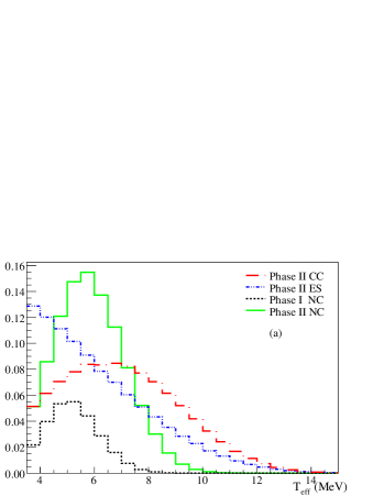
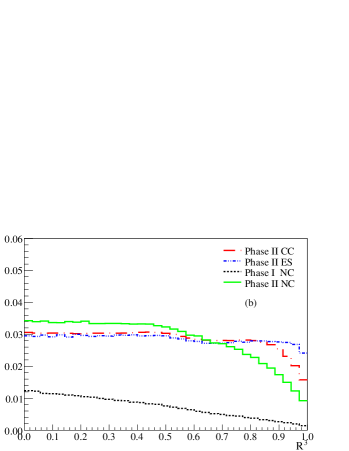
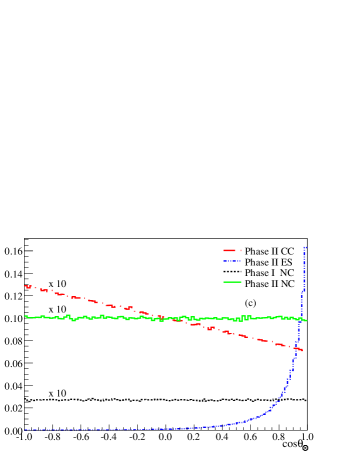
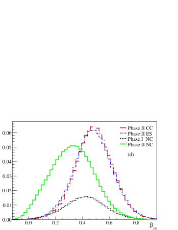
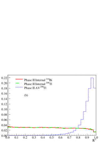
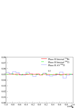
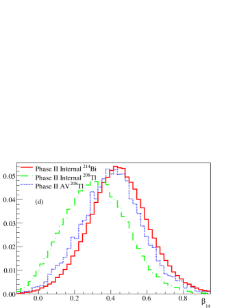
Figure 2 shows the same distributions for some of the detector backgrounds, namely ‘internal’ ²¹⁴Bi and ²⁰⁸Tl (within the D₂O volume) and ‘AV’ ²⁰⁸Tl (generated within the bulk acrylic of the vessel walls). While some of the ²¹⁴Bi nuclei came from decays of intrinsic ²³⁸U, the most likely source of ²¹⁴Bi was from decays of ²²²Rn entering the detector from mine air. The ²⁰⁸Tl nuclei came largely from decays of intrinsic ²³²Th. Near the $T_{\rm eff}=3.5$ MeV threshold the dominant signal was from events originating from radioactive decays in the PMTs. These events could not be generated with sufficient precision using the simulation, and so were treated separately from other event types, as described in Sec. XIII.3. There were many other backgrounds; these are described in Sec. XIII.

Figure 2: (Color online) The Monte Carlo-generated distributions of (a) energy ($T_{\rm eff}$) on a log scale, (b) radius cubed ($R^{3}$), (c) direction ($\cos\theta_{\odot}$), and (d) isotropy ($\beta_{14}$) for background events. The same simulation was used to build multi-dimensional PDFs to fit the background events. The backgrounds shown are internal ²¹⁴Bi, internal ²⁰⁸Tl, and AV ²⁰⁸Tl.

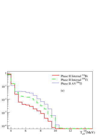
The energy spectra provide a powerful method for separating different event types. The CC and ES spectra depend on the shape of the incident neutrino spectrum. We treated the CC and ES spectra in two different ways: in one fit we made no model assumptions about the underlying spectral shape, allowing the CC and ES spectra to vary in the fit, and in a second fit we assumed that the underlying incident neutrino spectrum could be modeled as a smoothly distorted ⁸B spectrum. The shapes of NC and background spectra do not depend on neutrino energy and so were fixed in the fit, to within the systematic uncertainties derived later. Decays of ²¹⁴Bi and ²⁰⁸Tl in the detector both led to $\gamma$ rays above the deuteron binding energy of 2.2 MeV, which created higher energy events when the photodisintegration neutron was subsequently captured on either deuterium (Phase I) or predominantly ³⁵Cl (Phase II). A significant fraction of ²¹⁴Bi decays produce a 3.27 MeV-endpoint $\beta$. These background events are therefore characterized by steeply falling energy spectra with a photodisintegration tail, as shown in Fig. 2(a).

CC and ES events produced single electrons and, hence, the observed light from these events was fairly anisotropic, yielding a correspondingly high value for the isotropy parameter, $\beta_{14}$. The $\beta_{14}$ distributions show small differences due to the different energy spectra of the two event types, which affects $\beta_{14}$ through the known correlation between energy and isotropy of an event. The isotropy of Phase I NC events looks similar to that of CC and ES events, because the $\gamma$ ray tended to produce light dominated by that from one Compton electron. By contrast, the isotropy distribution of Phase II NC events is peaked noticeably lower because neutron capture on ³⁵Cl atoms nearly always resulted in multiple $\gamma$s, which could each scatter an electron and, hence, produce a more isotropic PMT hit pattern. Therefore, $\beta_{14}$ provides a sensitive method for separation of electron-like events from neutron capture events in this phase, without requiring a constraint on the shapes of the CC and ES energy spectra, thus providing an oscillation-model-independent measurement of the flux of solar neutrinos. The isotropy distributions for ²¹⁴Bi events and ²⁰⁸Tl events inside the heavy water are noticeably different because, above the $T_{\rm eff}=$ 3.5 MeV threshold, Cherenkov light from ²¹⁴Bi events was dominated by that from the ground state $\beta$ branch while that from ²⁰⁸Tl events was from a $\beta$ and at least one additional Compton electron. The difference allowed these events to be separated in our fit, as was done in previous SNO in-situ estimates of detector radioactivity longd2o ; nsp .

The $\cos\theta_{\odot}$ distribution is a powerful tool for distinguishing ES events since the scattering of $\nu_{e}$ from the Sun resulted in electron events whose direction is strongly peaked away from the Sun’s location. The direction of CC events displays a weaker correlation of $\sim(1-\frac{1}{3}$$\cos\theta_{\odot}$) relative to the direction of the Sun. The NC distribution is flat since the $\gamma$s generated by neutron capture carried no information about the incident neutrino direction. Background events had no correlations with the Sun’s location and, thus, also exhibit a flat distribution, as shown in Fig. 2(c).

The radial position of events within the detector yields a weak separation between the three neutrino interaction types, but a much more powerful level of discrimination from external background events. CC and ES events occurred uniformly within the detector and hence have relatively flat distributions. NC events occurred uniformly, but neutrons produced near the edge of the volume were more likely to escape into the AV and H₂O regions, where the cross section for neutron capture was very high due to the hydrogen content. Neutron capture on hydrogen produced 2.2 MeV $\gamma$s, below the analysis threshold and thus less likely to be detected. Therefore, the radial profile of NC events falls off at the edge of the volume. This effect is more noticeable in Phase I, since the neutron capture efficiency on deuterium is lower than on ³⁵Cl and, hence, the neutron mean-free path was longer in Phase I than in Phase II.

III Analysis Overview

The ‘LETA’ analysis differs from previous SNO analyses in the joint fit of two phases of data, the much lower energy threshold, (which both result in increased statistics) and significantly improved systematic uncertainties.

The neutrino signal rates were determined by creating probability density functions (PDFs) from distributions like those in Figs. 1 and 2 and performing an extended maximum likelihood fit to the data. The CC and ES spectra were determined by either allowing the flux to vary in discrete energy intervals (an ‘unconstrained fit’) or by directly parameterizing the $\nu_{e}$ survival probability with a model and fitting for the parameters of the model.

There were three major challenges in this analysis: reduction of backgrounds, creation of accurate PDFs (including determination of systematic uncertainties on the PDF shapes), and extracting the neutrino signals, energy spectra, and survival probabilities from the low-threshold fits.

Three new techniques were applied to reduce backgrounds compared to previous SNO analyses longd2o ; nsp . First, we made substantial improvements to energy reconstruction by developing a new algorithm that included scattered and reflected light in energy estimation. The inclusion of ‘late light’ narrowed the detector’s effective energy resolution by roughly 6%, substantially reducing the leakage of low-energy background events into the analysis data set by $\sim$60%. Second, we developed a suite of event-quality cuts using PMT charge and time information to reject external background events whose reconstructed positions were within the fiducial volume. Third, we removed known periods of high radon infiltration that occurred during early SNO runs and when pumps failed in the water purification system.

Creation of the PDFs was done primarily with a Monte Carlo (MC) simulation that included a complete model of physics processes and a detailed description of the detector. We made substantial improvements to the Monte Carlo model since our previous publications, and we describe these improvements in detail in Sec. V.

Our general approach to estimating systematic uncertainties on the Monte Carlo-simulated PDF shapes was based on a comparison of calibration source data to Monte Carlo simulation, as in previous SNO analyses. In cases where the difference between calibration data and simulation was inconsistent with zero, and we had evidence that the difference was not caused by a mis-modeling of the calibration source, we corrected the PDF shapes to better match the data. For example, we applied corrections to both the energy (Sec. VIII) and isotropy (Sec. IX) of simulated events. Any residual difference was used as an estimate of the uncertainty on the Monte Carlo predictions. Corrections were verified with multiple calibration sources, such as the distributed ‘spike’ sources as well as encapsulated sources, and additional uncertainties were included to account for any differences observed between the various measurements. Uncertainties were also included to take into account possible correlations of systematic effects with the observable parameters. So, for example, we allowed for an energy dependence in the fiducial volume uncertainty, and the uncertainty on the energy scale was evaluated in a volume weighted fashion to take into account possible variations across the detector.

The final extraction of signal events from the data was a multi-dimensional, many-parameter fit. Although marginal distributions like those shown in Figs. 1 and 2 could be used as PDFs, in practice there are non-trivial correlations between the observables that can lead to biases in the fit results. We therefore used three-dimensional PDFs for most of the backgrounds and for the NC signal, factoring out the dimension in $\cos\theta_{\odot}$, which is flat for these events. The CC and ES events had PDFs whose dimensionality depended on the type of fit. For the unconstrained fit, we used three-dimensional PDFs in $(R^{3},\beta_{14},\cos\theta_{\odot})$, factoring out the $T_{\rm eff}$ dimension because the fit was done in discrete intervals, within which the $T_{\rm eff}$ spectrum was treated as flat. For the direct fit for the $\nu_{e}$ survival probability, we used fully four-dimensional PDFs for the CC and ES signals.

The parameters of the ‘signal extraction’ fits were the amplitudes of the signals and backgrounds, as well as several parameters that characterized the dominant systematic uncertainties. A priori information on backgrounds and systematic uncertainties was included. To verify the results, we pursued two independent approaches, one using binned and the other unbinned PDFs. We describe both approaches in Sec. XIV.

We developed and tuned all cuts using simulated events and calibration source data. Signal extraction algorithms were developed on Monte Carlo ‘fake’ data sets, and tested on a 1/3-livetime sample of data. Once developed, no changes were made to the analysis for the final fit at our analysis threshold on the full data set.

In treating systematic uncertainties on the PDF shapes, we grouped the backgrounds and signals into three classes: ‘electron-like’ events, which include true single-electron events as well as those initiated via Compton scattering from a single $\gamma$; neutron capture events on chlorine that produced a cascade of many $\gamma$s with a complex branching table; and PMT $\beta$-$\gamma$ decays, which occurred in the glass or envelope of the PMT assembly and support structure. The PMT $\beta$-$\gamma$ events were treated separately from other $\beta$-$\gamma$ events because they were heavily influenced by local optical effects near the PMT concentrators and support structure, and are therefore hard to model or simulate.

The analysis results presented here have substantially reduced uncertainties on the neutrino interaction rates, particularly for SNO’s signature neutral current measurement. Although there are many sources of improvement, the major causes are:

• The lower energy threshold increased the statistics of the CC and ES events by roughly 30%, and of the NC events by $\sim 70$%;

• In a joint fit, the difference in neutron detection sensitivity in the two phases provided improved neutron/electron separation, beyond that due to differences in the isotropy distributions;

• Significant background reduction due to improved energy resolution, removal of high radioactivity periods, and new event quality cuts;

• Use of calibration data to correct the PDF shapes.

IV Data Sets

The Phase I and Phase II data sets used here have been described in detail elsewhere longd2o ; nsp . We note only a few critical details.

SNO Phase I ran from November 2, 1999 to May 31, 2001. Periods of high radon in Phase I were removed for this analysis based on the event rate. To minimize bias, we used Chauvenet’s criterion to eliminate runs in which the probability of a rate fluctuation as high or higher than observed was smaller than 1/(2$N$), where $N$ is the total number of runs in our data set ($\sim 500$). With this cut, we reduced the previously published 306.4 live days to 277.4. Most of the runs removed were in the first two months of the phase, or during a period in which a radon degassing pump was known to have failed. This $\sim$9% reduction in livetime removed roughly 50% of all ²¹⁴Bi events from the Phase I data set. SNO Phase II ran from July 2001 to August 2003, for a total of 391.4 live days.

SNO had several trigger streams, but the primary trigger for physics data required a coincidence of $N_{\rm coinc}$ or more PMT hits within a 93 ns window. From the start of Phase I until December 20, 2000, $N_{\rm coinc}$ was set to 18; it was subsequently lowered to 16 PMT hits. This hardware threshold is substantially below the analysis threshold, and no efficiency correction was required, even at 3.5 MeV (see Sec. XI).

V Monte Carlo Simulation

SNO’s Monte Carlo simulation played a greater role here than in previous publications, as we used it to provide PDFs of not only the neutrino signals, but for nearly all backgrounds as well. The simulation included a detailed model of the physics of neutrino interactions and of decays of radioactive nuclei within the detector. Propagation of secondary particles was done using the EGS4 shower code egs , with the exception of neutrons, for which the MCNP mcnp neutron transport code developed at Los Alamos National Laboratory was used. Propagation of optical photons in the detector media used wavelength-dependent attenuations of D₂O and H₂O that were measured in situ with laserball calibrations, and acrylic attenuations measured ex situ. The simulation included a detailed model of the detector geometry, including the position and orientation of the PSUP and the PMTs, the position and thickness of the AV (including support plates and ropes), the size and position of the AV ‘neck’, and a full three-dimensional model of the PMTs and their associated light concentrators. SNO’s data acquisition system was also simulated, including the time and charge response of the PMTs and electronics. Details of the simulation have been presented in longd2o ; nsp ; we describe here the extensive upgrades and changes that were made for this analysis.

Ultimately, SNO’s ability to produce accurate PDFs depends on the ability of the Monte Carlo simulation to reproduce the low-level characteristics of the data, such as the distributions of PMT hit times and charges. We therefore improved our timing model to more correctly simulate the ‘late pulsing’ phenomenon seen in the Hamamatsu R1408s used by SNO. We also added a complete model of the PMT single photoelectron charge distribution that includes PMT-to-PMT variations in gain. Gain measurements were made monthly with the laserball source at the center of the detector, and the simulation uses different charge distributions for each PMT according to these gain measurements.

Addition of the more complete charge spectrum also allowed us to add a detailed model of each electronics channel’s discriminator. On average, the threshold voltage was near 1/4 of that for a single photoelectron, but there were large variations among channels because of variations in noise level. Over time, the channel thresholds were adjusted as PMTs became quieter or noisier; these settings were used in the simulation for each run. The discriminator model also provided for channel-by-channel efficiencies to be included, thus improving simulation of the detector’s energy resolution.

We made several important changes to the optical model as well. The first was a calibration of PMT efficiencies, which accounted for tube-to-tube variations in the response of the photomultipliers and light concentrators. These efficiencies are distinct from the electronics discriminator efficiency described above, as they depended on the PMT quantum efficiency, local magnetic field, and individual concentrator reflectivity, while the discriminator efficiency depended upon PMT channel gain and threshold setting. The PMT efficiencies were measured using the laserball, as part of the detector’s full optical calibrations, which were performed once in Phase I and three times in Phase II. The efficiencies in the simulation were varied over time accordingly.

The light concentrators themselves are known to have degraded over time and the three-dimensional model of the collection efficiency of the PMT-concentrator assembly used in previous analyses had to be modified. We developed for this analysis a phenomenological model of the effects of the degradation to the concentrator efficiency. Rather than modifying the concentrator model itself, we altered the PMT response as a function of the position at which the photon struck the photocathode. In effect, this produced a variation in the response of the concentrator and PMT assembly as a function of photon incidence angle. A simultaneous fit was performed to laserball calibration data at six wavelengths, with each wavelength data set weighted by the probability that a photon of that wavelength caused a successful PMT hit. The extraction of optical calibration data was extended to a larger radius than in previous analyses, in order to extract the PMT response at wider angles. Ex-situ data were also included in the fit to model the response at $>\,$40^∘ for events in the light water region. Time dependence was accommodated by performing separate fits in time intervals defined by the available calibration data: one interval in Phase I and three in Phase II. This change improved the modeling of any position-dependence of the energy response but did not affect the overall energy scale, which was calibrated using the ¹⁶N source. We also made a global change to the light concentrator reflectivity based on measurements with the ¹⁶N source. Figure 3 compares the new model of the PMT-concentrator response as a function of incidence angle to that used in earlier publications.

Figure 3: (Color online) Comparison of new model of photomultiplier angular response to data and the old model for Phase I at 365 nm.

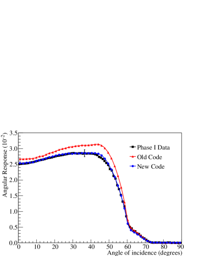
The laserball calibration data were used as a direct input to the energy reconstruction algorithms, providing media attenuations, PMT angular response measurements, and PMT efficiencies. For wavelengths outside the range in which data were taken, the Monte Carlo simulation was used to predict the response.

VI Hit-level Calibrations

The accuracy with which we know the charge and time of each PMT hit directly affects event position and energy uncertainties. To calibrate the digitized charges and time, we performed pulser measurements twice weekly, measuring pedestals for the charges and the mapping of ADC counts to nanoseconds for the times. The global channel-to-channel time offsets and the calibration of the pulse risetime corrections were done with the laserball source deployed near the center of the detector. These calibrations have been described elsewhere longd2o .

Four significant changes were made to the calibration of PMT charges and times. The first was the removal of hits associated with channel-to-channel crosstalk. Crosstalk hits in the SNO electronics were characterized by having low charges, slightly late times, and being adjacent to a channel with very high charge.

The second change was a correction to the deployed positions of the laserball source to ensure that the time calibrations were consistent between calibration runs. Prior to this correction, the global PMT offsets had been sensitive to the difference between the nominal and true position of the source, which varied from calibration run to calibration run. The new correction reduced the time-variations of the PMT calibrations noticeably, but there was a residual 5 cm offset in the reconstructed $z$-position of events, for which a correction was applied to all data.

There were a variety of ways in which PMTs could fail, and we therefore applied stringent criteria for a PMT to be included in position and energy reconstruction. The criteria were applied to both calibration and ‘neutrino’ data sets as well as to run simulations.

The last improvement was a calibration to correct for a rate-dependence in the electronics charge pedestals. Crosstalk hits were used to monitor the pedestal drift and a time-varying correction was applied. With this correction we could use the PMT charge measurements to remove certain types of background events, and to substantially reduce systematic uncertainties on the energy scale associated with variations in PMT gain, which affected the photon detection probability.

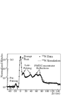
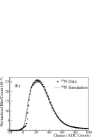
Figure 4 shows the distributions of PMT time-of-flight residuals and measured photoelectron charges for a ¹⁶N calibration run at the center of the detector compared to a simulation of that run. The simulation includes the upgrades discussed in Sec. V. The time residuals show excellent agreement in the dominant prompt peak centered near $\Delta t=0$ ns, as well as good agreement for the much smaller pre-pulsing ($\Delta t\sim-20$ ns) and late-pulsing ($\Delta t\sim 15$ ns and $\Delta t\sim 35$ ns) features. For the charge distribution, the agreement is also excellent above 10 ADC counts or so, which corresponds to the majority of the charges used in the analysis. Thus, we are confident that the simulation models the behavior of reconstruction and cuts with sufficient accuracy.

Figure 4: Comparison of ¹⁶N simulation to data for (a) PMT hit time-of-flight residuals and (b) photoelectron charge spectra.

VII Position and Direction Reconstruction

The primary reconstruction algorithm used in this analysis was the same as in previous Phase I publications. We used reconstructed event position and direction to produce the PDFs shown in Figs. 1 and 2, and to reject background events originating outside the AV. Knowledge of event position and direction was also used in the estimation of event energy (see Sec. VIII). Below we outline the reconstruction method, and then discuss the uncertainties in our knowledge of event positions and directions.

VII.1 Reconstruction Algorithm

The vertex and direction reconstruction algorithm fitted event position, time, and direction simultaneously using the hit times and locations of the hit PMTs. These values were found by maximizing the log-likelihood function,

$${\log\cal L}(\vec{r}_{e},\vec{v}_{e},t_{e})=\sum_{i=1}^{N_{\rm hit}}\log{\cal P}(t^{\rm res}_{i},\vec{r}_{i};\vec{r}_{e},\vec{v}_{e},t_{e}),$$ (1)

with respect to the reconstructed position ($\vec{r}_{e}$), direction ($\vec{v}_{e}$), and time ($t_{e}$) of the event. ${\cal P}(t^{\rm res}_{i},\vec{r}_{i};\vec{r}_{e},\vec{v}_{e},t_{e})$ is the probability of observing a hit in PMT $i$ (located at $\vec{r}_{i}$) with PMT time-of-flight residual $t^{\rm res}_{i}$ (Eq. (2)), given a single Cherenkov electron track occurring at time $t_{e}$ and position $\vec{r}_{e}$, with direction $\vec{v}_{e}$. The sum is over all good PMTs for which a hit was recorded. The PMT time-of-flight residuals relative to the hypothesized fit vertex position are given by:

$$t^{\rm res}_{i}=t_{i}-t_{\rm e}-|\vec{r}_{\rm e}-\vec{r}_{i}|\frac{{n_{\rm eff}}}{c},$$ (2)

where $t_{i}$ is the hit time of the $i$th PMT. The photons are assumed to travel at a group velocity $\frac{{c}}{n_{\rm eff}}$, with ${n_{\rm eff}}$ an effective index of refraction averaged over the detector media.

The probability ${\cal P}$ contains two terms to allow for the possibilities that the detected photon arrived either directly from the event vertex (${\cal P}_{\rm direct}$) or resulted from reflections, scattering, or random PMT noise (${\cal P}_{\rm other}$). These two probabilities were weighted based on data collected in the laserball calibration runs.

The azimuthal symmetry of Cherenkov light about the event direction dilutes the precision of reconstruction along the event direction. Thus, photons that scattered out of the Cherenkov cone tended to systematically drive the reconstructed event vertex along the fitted event direction. After initial estimates of position and direction were obtained, a correction was applied to shift the vertex back along the direction of the event so as to compensate for this systematic drive. The correction varied with the distance of the event from the PSUP as measured along its fitted direction.

The reconstruction algorithm returned a quality-of-fit statistic relative to the hypothesis that the event was a correctly reconstructed single electron. This statistic was used later in the analysis to remove backgrounds and reduce tails on the reconstruction resolution. Details of the reconstruction algorithm can be found in longd2o .

VII.2 Uncertainties on Position and Direction

Many effects that could produce systematic shifts in reconstructed positions were modeled in the simulation. Data from calibration sources deployed within the detector were compared to Monte Carlo predictions, and the differences were used to quantify the uncertainty on the simulation. The observed differences were not deemed significant enough to warrant applying a correction to the Monte Carlo-generated positions, and so the full size of the difference was taken as the magnitude of the uncertainty. The differences between data and Monte Carlo events were parameterized as four types:

• vertex offset: a constant offset between an event’s true and reconstructed positions;

• vertex scale: a position-dependent shift of events either inward or outward;

• vertex resolution: the width of the distribution of reconstructed event positions;

• angular resolution: the width of the distribution of reconstructed event directions relative to the initial electron direction.

These uncertainties can have an impact upon the flux and spectral measurements in two ways: by altering the prediction for the number of events reconstructing inside the fiducial volume and by affecting the shape of the PDFs used in the signal extraction.

Reconstruction uncertainties were determined primarily from ¹⁶N source data. In previous analyses longd2o , the volume density of Compton-scattered electrons relative to the source location was modeled with the analytic function $S(r)\sim\exp(\frac{-r}{\lambda})/(r^{2})$. Model improvements for this analysis allowed us to extract this distribution for each ¹⁶N source run from the Monte Carlo simulation of that run, and take into account the exact source geometry, effect of data selection criteria on the distribution, and any time-dependent detector effects.

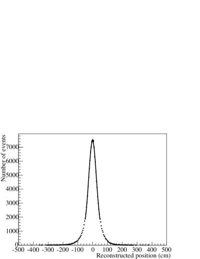
The distribution of electron positions was convolved with a Gaussian, representing the detector response, and the resulting function was fit to the one-dimensional reconstructed position distribution along each axis, allowing both the mean and standard deviation of the Gaussian to vary for each orthogonal axis independently. An example of such a fit is shown in Figure 5. This fit was done separately for the ¹⁶N data and the Monte Carlo simulation of each ¹⁶N run. The difference in the Gaussian means gives the vertex offset for that run and the square root of the difference in the variances represents the difference in vertex resolution.

Figure 5: Fit of the ¹⁶N Compton-electron position distribution convolved with a Gaussian to the reconstructed $z$ position of ¹⁶N data events for a typical central run in Phase II.

VII.2.1 Vertex Offset

Analysis of the differences between the reconstructed and true event vertex positions at the center of the detector, or ‘central vertex offset’, was done using runs with the source within 25 cm of the center, where the source position is known most accurately. This avoids confusion with any position-dependent effects, which are taken into account in the scale measurement (Sec. VII.2.2). A data$-$MC offset was determined for each run, along each detector axis. The offsets from the runs were combined in weighted averages along each axis, with the uncertainty for each run offset increased to include the uncertainty in source position. Although the results showed a small mean offset along each axis, the magnitude was comparable to the source position uncertainty and therefore we did not correct the PDFs based on this difference. Instead, asymmetric double-sided uncertainties were formulated by using the uncertainty in the weighted average, and increasing it by the magnitude of the weighted average itself on the side on which the offset was measured. The effects of these uncertainties were determined during signal extraction by shifting the position of each event by the positive and negative values of the uncertainty along each axis independently, and recomputing the PDFs. The values of the uncertainties are given in Table 2 in Sec. VII.2.6.

VII.2.2 Vertex Scale

A potential position-dependent bias in the reconstructed position that can be represented as being proportional to the distance of the event from the center of the detector is defined as a vertex scale systematic.

In previous SNO analyses, uncertainty in the position of the calibration source was a major contribution to reconstruction uncertainties, especially away from the $z$-axis of the detector, where sources were deployed in a less accurate mode. A new method was derived for this analysis to reduce sensitivity to this effect. Although the absolute source position was known only to $\sim 2\,$cm on the $z$-axis and $\sim 5\,$cm away from this axis, changes in position once the source was deployed were known with much greater precision. By comparing the result from each ¹⁶N run to a run at the center of the detector from the same deployment scan, possible offsets between the recorded and true source position were removed, thus reducing source position uncertainties. In addition, any constant offset in vertex position, such as that measured in Sec. VII.2.1, was inherently removed by this method, thus deconvolving the measurement of scale from offset. This method allowed data from different scans to be combined, providing a more representative sampling across the time span of the data set and improving the statistics of the measurement.

Vertex scale was investigated by using the data$-$MC reconstructed position offset along each detector axis, as shown in Figure 6, using only runs within 50 cm of that axis to minimize correlations among the three. The runs were grouped into 50 cm bins along each axis by source position, and the weighted average of the offsets for the runs within each bin was found. A linear function was fit to the bins as a function of position along that axis. Since the method was designed to remove any central vertex offset, the function was defined to be zero at the center of the detector.

Figure 6: (Color online) Vertex offset along the three detector axes as a function of position within the detector.

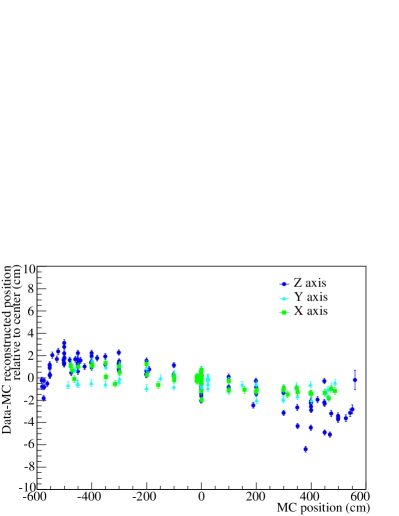
The slope from the fit provides the scaling required to bring the simulation into agreement with data. We did not apply a correction, but instead treated it as an asymmetric uncertainty on the reconstructed positions of all events. The effects observed along the $x$ and $y$ axes were of a very similar magnitude and, therefore, were assumed to be due to a radial effect, possibly caused either by small errors in the modeling of the wavelength-dependent refractive index or residual PMT timing calibration errors. Conservatively, the larger of the $x$ and $y$ values was used to bound this effect. The resulting uncertainty was applied in our signal extraction fits by multiplying the $x$, $y$ and $z$ position of each event in our PDFs by the value of the scale uncertainty, thus shifting events either inwards or outwards in the detector, and taking the difference from the nominal fit. Since the effect observed along the $z$-axis was larger, the difference of this from the radial effect was treated as an additional uncertainty, applied only to the $z$ position of events. The values used for each uncertainty are listed in Table 2 in Sec. VII.2.6.

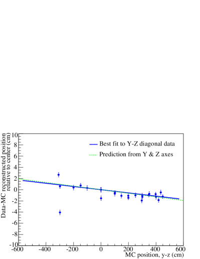
Since only runs within 50 cm of each Cartesian axis were used to determine vertex scale, diagonal axis runs could be used for verification. The method described measured the scale for each Cartesian axis independently. The values obtained for the $y$ and $z$ axes, for example, could therefore be combined to predict the scaling for runs on the $y$-$z$ diagonal. The prediction was shown to agree very well with the data, as illustrated in Figure 7, demonstrating the robustness of the analysis and its applicability to events everywhere in the fiducial volume.

Figure 7: (Color online) Vertex offset along the $y$-$z$ diagonal as a function of position along that diagonal. The dashed line shows the prediction from the $y$- and $z$-axis values and the solid line shows the best fit scaling value for these data points. Observed variations at negative positions are likely associated with systematics in source position.

A similar analysis was performed using ²⁵²Cf source data in Phase II. The results were consistent with those shown here, verifying that the same uncertainties could be applied to both electron-like and neutron capture events.

We investigated several other potential causes of variation in reconstruction accuracy. The ¹⁶N-source event rate during most calibration runs was high in comparison to our expected neutrino event rate, so the results were checked using low-rate ¹⁶N data. The stability over time was determined by comparing runs across the span of the two phases. As in previous analyses longd2o , calibration-source dependence was investigated by verifying ¹⁶N results using the ⁸Li source. This also provides a check on the energy dependence because the ⁸Li data extended to higher energies than the ¹⁶N data. The results were all consistent within the uncertainties presented here.

VII.2.3 Vertex Resolution

The position resolution achieved in this analysis was $\sim$20 cm for data events. The difference in resolutions between data and Monte Carlo events was modeled as a Gaussian of standard deviation (or ‘width’) $\sigma_{\rm extra}$, by which the Monte Carlo distribution should be smeared to reproduce the data. $\sigma_{\rm extra}^{2}$ was given by $(\sigma_{\rm Data}^{2}-\sigma_{\rm MC}^{2})$ for each ¹⁶N run. This procedure is only valid for $\sigma_{\rm MC}<\sigma_{\rm Data}$, which was the likely scenario since any minor detector non-uniformities tend to cause a broader resolution in the data. In some cases, the simulation and data were close enough to one another that statistical variation caused $\sigma_{\rm Data}$ to appear to be less than $\sigma_{\rm MC}$. In these cases, $|(\sigma_{\rm Data}^{2}-\sigma_{\rm MC}^{2})|$ was taken to represent the uncertainty in the comparison. The results from the runs were combined in a weighted average, independently for each detector axis. The resulting values for $\sigma_{\rm extra}$ are listed in Table 2 in Sec. VII.2.6. These were applied during the signal extraction by smearing the positions of all Monte Carlo events by a Gaussian of the appropriate width. This was achieved for the binned signal extraction (Sec. XIV.2) by generating a random number for each event from a Gaussian of the correct width and adding the result to the event’s position and, for the unbinned method, by a direct analytic convolution (Sec. XIV.3).

VII.2.4 Angular Resolution

The ¹⁶N source was used for this measurement by relying on the high degree of colinearity of Compton scattered electrons with the initial $\gamma$ direction. The mean of the distribution of reconstructed event positions was used to estimate the source position. The reconstructed event position was used as an estimate for the scattering vertex. To reduce the effect of reconstruction errors, only events reconstructing more than 120 cm from the source were used. The angle between the initial $\gamma$ direction (taken to be the vector from the source position to the fitted scattering vertex) and the reconstructed event direction was found and the distributions of these angles were compared for data and Monte Carlo events.

The same functional form used in previous analyses nsp was fit to the distributions for data and Monte Carlo events within each run. The weighted average of the differences in the fitted parameters was computed across the runs and the resulting value used as an estimate of the uncertainty in angular resolution (given in Table 2, Sec. VII.2.6).

VII.2.5 Energy Dependent Fiducial Volume

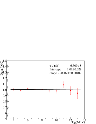
The energy dependence of the vertex scaling is of particular importance since it could affect the number of events that reconstruct within the fiducial volume as a function of energy and, hence, distort the extracted neutrino spectrum. Because the ¹⁶N source provided monoenergetic $\gamma$s, giving rise to electrons around 5 MeV, whereas the ⁸Li source sampled the full range of the neutrino energy spectrum, the ⁸Li source was used for this measurement. The fraction of events reconstructing inside the source’s radial position, closer to the detector center, was used as a measure of the number of events reconstructing inside the fiducial volume to take into account both vertex shift and resolution effects. Absolute offsets between data and Monte Carlo events have already been characterized in Sections VII.2.1–VII.2.3, so a differential comparison of this parameter between data and Monte Carlo events was used to evaluate any energy dependence. A fit from Phase II is shown in Figure 8. The energy dependence is given by the slope of a straight line fit to the ratio of the data and Monte Carlo parameters, averaged across calibration runs. The final uncertainty is quoted as an asymmetric, double-sided uncertainty to account for the non-zero value of the slope and its uncertainty. The values for each phase are given in Table 2. The absolute shift, indicated in Fig. 8 by an intercept different from one, is a measure of the global vertex scaling. This effect has already been evaluated in Sec. VII.2.2. It does not impact the energy dependence and therefore is not relevant to this present measurement.

Figure 8: (Color online) Ratio of the fraction of events reconstructing inside the source position for data and Monte Carlo events, as a function of effective electron energy, for ⁸Li source runs.

An additional check was performed using neutrino data from outside the fiducial volume. All standard analysis cuts were applied, as described in Sec. X, as well as a 5.5 MeV threshold to select a clean sample of neutrino events. A Hill function was fit to the radial distribution of the events, with the half-point of the function representing the position of the AV. Statistics in the data were limited, so the fit was performed in just three energy bins. Monte Carlo simulation of the three types of neutrino interactions was combined in the signal ratios found in a previous SNO analysis nsp and the same fit was performed. The ratio of the resulting fitted AV position in the data and simulation is a measure of the radial scaling and, therefore, the energy dependence of this ratio is a check on the analysis described above. The results were in good agreement. In Phase II the energy dependence was $0.8\pm 2.1\%$/MeV, in comparison to $-0.07\pm 0.41\%$/MeV measured using the ⁸Li source.

VII.2.6 Summary of Reconstructed Position Uncertainties

Table 2 summarizes the uncertainties in reconstructed position and direction.

	Uncertainty, $\delta_{i}$		Transformation
Parameter	Phase I	Phase II	of observables
$x$ Offset (cm)	${}^{+1.15}_{-0.13}$	${}^{+0.62}_{-0.07}$	$x+\delta_{i}$
$y$ Offset (cm)	${}^{+2.87}_{-0.17}$	${}^{+2.29}_{-0.09}$	$y+\delta_{i}$
$z$ Offset (cm)	${}^{+2.58}_{-0.15}$	${}^{+3.11}_{-0.16}$	$z+\delta_{i}$
$R$ Scale (%)	${}^{+0.10}_{-0.57}$	${}^{+0.04}_{-0.34}$	$(1+\frac{\delta_{i}}{100})x_{i}$
$z$ Scale (%)	${}^{+0.40}_{-0.0}$	${}^{+0.03}_{-0.25}$	$(1+\frac{\delta_{i}}{100})z$
$x$ resn (cm)	$+3.3$	$+3.1$	$x+\mathcal{N}(0,\delta_{i})$
$y$ resn (cm)	$+2.2$	$+3.4$	$y+\mathcal{N}(0,\delta_{i})$
$z$ resn (cm)	$+1.5$	$+5.3$	$z+\mathcal{N}(0,\delta_{i})$
Angular resn	$\pm 0.11$	$\pm 0.11$	$1+(\cos\theta_{\odot}-1)(1+\delta_{i})$
EFV (%/MeV)	${}^{+0.85}_{-0.49}$	${}^{+0.41}_{-0.48}$	$W=1+\frac{\delta_{i}}{100}(T_{\rm eff}-5.05)$

Table 2: Systematic uncertainties in the reconstructed position and direction of events. EFV is the energy dependent fiducial volume uncertainty. The column labeled “Transformation of observables” refers to the formulae used to propagate these uncertainties into the signal extraction fits. $\mathcal{N}(0,\delta_{i})$ refers to a convolution with a Gaussian distribution of mean 0.0 and standard deviation $\delta_{i}$. Events that are pushed past $\cos\theta_{\odot}$ $=\pm 1.0$ are randomly assigned a $\cos\theta_{\odot}$ value in the interval [-1.0, 1.0]. $W$ is an energy-dependent fiducial volume factor applied around the midpoint of the ¹⁶N energy, where $T_{\rm eff}$ is the reconstructed effective electron kinetic energy and 5.05 MeV is the central $T_{\rm eff}$ value for the ¹⁶N data. This was applied as a weight for each event when creating the PDFs. (“Resolution” is abbreviated as “resn”).

It is worth noting that in previous analyses nsp the radial scaling uncertainty was evaluated at $\pm\,$1%, which translates to a 3% uncertainty in fiducial volume. The improved analysis presented here has reduced the scale uncertainty to a little over 0.5% at its maximum and significantly less in most dimensions. The resolution differences observed previously were on the order of 9 cm longd2o , whereas the differences measured here are roughly one third of that in most dimensions. The angular resolution uncertainty of 11% is an improvement over the 16% measured in previous work nsp .

VIII Energy Reconstruction

We estimated the kinetic energy of an event after its position and direction were reconstructed. The energy estimate was used both to reject background events and to produce the PDFs shown in Figs. 1 and 2. Improving the resolution of the energy estimation algorithm was critical because of the low energy threshold of the analysis – a 6% improvement in energy resolution reduces the number of background events reconstructing above threshold by $\sim$60%.

VIII.1 Total-Light Energy Estimator

A new algorithm, called “FTK”, was designed to use all the detected PMT hits in the energy estimate, including scattered and reflected light dunfordthesis . The look-up table approach of the prompt-light fitter used in previous publications was abandoned in favor of a maximum likelihood method, in which photon detection probabilities were generated based on the reconstructed event position and direction. The best value of the effective kinetic energy, $T_{\rm eff}$, was found by maximizing the likelihood given the observed number of hit PMTs, $N_{\rm hit}$, and taking into account optical effects due to the reconstructed position and direction of the event. In principle, one could consider a more sophisticated approach in which both the number and distribution of all hit PMTs are used along with the recorded time of each hit, but such an approach is much more time intensive and was judged to be impractical for the present analysis.

We considered five sources of PMT hits in an event, defined by the following quantities:

• $n^{\rm dir}_{\rm exp}$ - the expected number of detected photons that traveled directly to a PMT, undergoing only refraction at the media boundaries;

• $n^{\rm scat}_{\rm exp}$ - the expected number of detected photons that were Rayleigh scattered once in the D₂O or H₂O before detection (scattering in the acrylic is neglected);

• $n^{\rm av}_{\rm exp}$ - the expected number of detected photons that reflected off the inner or outer surface of the acrylic vessel;

• $n^{\rm pmt}_{\rm exp}$ - the expected number of detected photons that reflected off the PMTs or light concentrators;

• $n^{\rm noise}_{\rm exp}$ - the expected number of PMT noise hits, based on run-by-run measurements.

FTK computed the probabilities of a single photon being detected by any PMT via the four event-related processes: $\rho_{\rm dir}$, $\rho_{\rm scat}$, $\rho_{\rm av}$, $\rho_{\rm pmt}$. The direct light probability was found by tracing rays from the event vertex to each PMT, and weighting each ray by the attenuation probability in each medium, transmittance at each boundary, solid angle of each PMT, and detection probability given the angle of entry into the light concentrator. Scattering and reflection probabilities were found using a combination of ray tracing and tables computed from Monte Carlo simulation of photons propagating through the detector.

If $N_{\gamma}$ is the number of potentially detectable Cherenkov photons produced in the event given the inherent PMT detection efficiency, then the expected number of detected photons given these probabilities is:

$$n_{\rm exp}(N_{\gamma})=N_{\gamma}\times(\rho_{\rm dir}+\rho_{\rm scat}+\rho_{\rm av}+\rho_{\rm pmt}).$$ (3)

To be able to compare $n_{\rm exp}$ to the observed $N_{\rm hit}$, we need to account for noise hits and convert from detected photons to PMT hits, since multiple photons in the same PMT produced only one hit. Given the rarity of multiple photons in a single PMT at solar neutrino energies, FTK made a correction only to the dominant source term, $n^{\rm dir}_{\rm exp}=N_{\gamma}\rho_{\rm dir}$. Letting $N_{\rm MPC}(n^{\rm dir}_{\rm exp})$ be the multi-photon corrected number of direct PMT hits, the total expected number of hits is:

$$N_{\rm exp}(N_{\gamma}) \approx N_{\rm MPC}(n^{\rm dir}_{\rm exp})$$ (4)

$$+N_{\gamma}\times(\rho_{\rm scat}+\rho_{\rm av}+\rho_{\rm pmt})+n^{\rm noise}_{\rm exp}.$$

The probability of observing $N_{\rm hit}$ hits when $N_{\rm exp}$ are expected is given by the Poisson distribution:

$$P(N_{\rm hit}\,|\,N_{\gamma})=\frac{(N_{\rm exp})^{N_{\rm hit}}e^{-N_{\rm exp}}}{N_{\rm hit}!}.$$ (5)

To obtain a likelihood function for $T_{\rm eff}$, rather than $N_{\gamma}$, we integrate over the distribution of $N_{\gamma}$ given an energy $T_{\rm eff}$:

$$\mathcal{L}(T_{\rm eff})=\int\frac{(N_{\rm exp}(N_{\gamma}))^{N_{\rm hit}}e^{-N_{\rm exp}(N_{\gamma})}}{N_{\rm hit}!}\times P(N_{\gamma}\,|\,T_{\rm eff})\,dN_{\gamma},$$ (6)

where $P(N_{\gamma}\,|\,T_{\rm eff})$ is the probability of $N_{\gamma}$ Cherenkov photons being emitted in an event with energy $T_{\rm eff}$. The negative log-likelihood was then minimized in one dimension to give the estimated energy of the event.

VIII.2 Energy Scale Corrections and Uncertainties

We measured the energy scale of the detector by deploying the tagged ¹⁶N $\gamma$ source at various locations in the $x$-$z$ and $y$-$z$ planes within the D₂O volume. Although ¹⁶N was a nearly monoenergetic $\gamma$ source, it produced electrons with a range of energies through multiple Compton scattering and $e^{+}e^{-}$ pair production. As a result, the single 6.13 MeV $\gamma$ produced an ‘effective electron kinetic energy’ ($T_{\rm eff}$) distribution that peaked at approximately 5 MeV.

Using the ¹⁶N $\gamma$-ray source to determine the detector’s energy scale is complicated by its broad spectrum of electron energies. To separate the detector’s response from this intrinsic electron energy distribution, we modeled the reconstructed energy distribution with the integral

$$P(T_{\rm eff})=N\int P_{\rm source}(E_{e^{-}})\frac{1}{\sqrt{2\pi}\,\sigma}e^{\frac{(T_{\rm eff}-E_{e^{-}}-p_{3})^{2}}{2\sigma^{2}}}dE_{e^{-}},$$ (7)

where $N$ is a normalization constant, $\sigma(E_{e^{-}})=p_{1}+p_{2}\sqrt{E_{e^{-}}}$ is the detector resolution, and $P_{\rm source}$ is the apparent electron energy distribution from the ¹⁶N $\gamma$ rays without including the detector optical response. $p_{3}$ sets the displacement of the ¹⁶N peak, and therefore the offset in energy scale at that source location. The $P_{\rm source}$ distribution was computed from a Monte Carlo simulation of $\gamma$ propagation through the source container and production of Cherenkov photons from Compton-scattered $e^{-}$ and pair-produced $e^{+}e^{-}$. We translated the number of Cherenkov photons in each simulated event to a most probable electron (MPE) kinetic energy with the same tables that were used in the FTK energy estimation algorithm, and generated the distribution, $P_{\rm source}$, of event values dunfordthesis . Given this fixed distribution for the ¹⁶N calibration source, we fit for $N$, $p_{1}$, $p_{2}$, and $p_{3}$ in each source run, for both data and for Monte Carlo simulation of the same source position and detector state. The parameter differences between data and Monte Carlo, run-by-run, determined the energy corrections and uncertainties. Parameters $p_{1}$ and $p_{2}$ measure the detector energy resolution, and are discussed further in Sec. VIII.3. Parameter $p_{3}$ was used here to define the spatial energy scale correction and uncertainties.

The Monte Carlo was initially tuned by adjusting a global collection efficiency parameter in the simulation to minimize the difference between data and Monte Carlo energy scales for ¹⁶N runs at the center of the detector. A series of additional corrections were then applied to the estimated energy of all the data and Monte Carlo events, to remedy known biases.

Approximations in FTK’s handling of multiple hits on a single tube lead to a small energy non-linearity, and we derived a correction for this by comparing the reconstructed energy for Monte Carlo events to their true energies. Similarly, the simple PMT optical model used by FTK produced a small radial bias in event energies and, again, comparison of reconstructed energies of Monte Carlo events to their true values were used to provide a correction.

Two additional corrections were based on evaluations of data. The first was to compensate for the degradation of the PMT light concentrators, which changed the detector’s energy response over time during Phase I. The degradation affected the fraction of light that was reflected off the PMT array. We tracked the variation using ¹⁶N runs taken at the center of the detector, and created a time-dependent correction to event energies that shifted their values by up to 0.4% dunfordthesis .

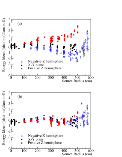
The final correction was applied to remove a variation in energy with the detector $z$-coordinate. Figure 9(a) shows the difference between the average reconstructed energies of events from the ¹⁶N source for each calibration run, and the Monte Carlo simulation of the run, as a function of the radial position of the source. As can be seen, for events in the top (positive $z$) hemisphere of the detector, the Monte Carlo underestimated the event energies by as much as 3% and, in the bottom hemisphere, it overestimated the energies by almost the same amount. The cause of the former was the simulation’s poor optical model of the acrylic in the neck of the AV. The latter was likely caused by accumulation of residue at the bottom of the acrylic vessel and variations in the degradation of the PMT light concentrators.

To correct for the $z$-dependence of the energy scale, we first split the ¹⁶N calibration runs into two groups. One group contained runs on the $x$-$z$ plane along with half of the runs on the $z$-axis, and was used to construct the correction function. The second group contained runs on the $y$-$z$ plane along with the other half of the $z$-axis runs, and was used later to independently evaluate the spatial component of the energy scale uncertainty.

We found that the variation in the energy scale best correlated with the vertical position of the event ($z$) and the direction cosine of the event relative to the $z$-axis ($u_{z}$). All of the ¹⁶N events in the first group were binned in the $(z,u_{z})$ dimensions and the peak of the ¹⁶N energy distribution was found for data and Monte Carlo events separately. We fit a second-order polynomial in $z$ and $u_{z}$ to the ratio of the data and Monte Carlo peak energies. This smooth function provided the spatial energy correction for data events. Fig. 9(b) shows the spatial variation after this energy correction.

Figure 9: (Color online) Difference between ¹⁶N data and Monte Carlo energy scales as a function of radius for Phase II ¹⁶N source runs in the upper hemisphere, on the equatorial plane, and in the lower hemisphere. Panel (a) shows the significant variation in these three regions before the spatial energy correction. Panel (b) shows the same runs after the spatial energy scale correction is applied. (The fiducial volume cut is at 550 cm).

To evaluate the spatial component of the energy scale uncertainty, we assumed azimuthal symmetry in the detector, and divided the second group of ¹⁶N calibration runs into regions based on radius and polar angle. Within each region, the RMS of the individual run differences between the corrected data and Monte Carlo energy scales defined the uncertainty on the energy scale in that volume. All regions were then combined into a volume-weighted measure of the uncertainty on the overall energy scale in the detector due to spatial variation and non-uniform sampling of the detector volume. As a verification of the procedure, we reversed the roles of the two calibration groups (using the $y$-$z$ plane to construct the calibration function and the $x$-$z$ plane to evaluate the uncertainties) and found very similar corrections and uncertainties.

The energy scale uncertainty of the detector also includes uncertainty in modeling of energy loss in the ¹⁶N source itself, uncertainties in the online status of PMTs, variation in the channel response between high-rate calibration data and low-rate neutrino data, and uncertainties in the data acquisition channel gains and thresholds, which affect the photon detection probability. Many of these uncertainties have been substantially reduced compared to previous publications by the improvements to the Monte Carlo model described in Sec. V and the rate-dependent correction to the channel pedestals described in Sec. VI.

The components of the energy scale uncertainties are summarized in Table 3. We take the source uncertainty as 100% correlated between phases, and the other uncertainties as uncorrelated. To verify the validity of the ¹⁶N-derived energy corrections and uncertainties over a wider range of energies, we compared the data and Monte Carlo energy distributions for ²⁵²Cf neutron source runs and the D₂O-volume radon spike, for both of which events are more widely distributed in the detector than for the ¹⁶N source. In both cases, the agreement between the data and Monte Carlo was well within the uncertainties stated in Table 3.

Uncertainty	Phase I	Phase II
PMT Status	$\pm 0.01$%	$\pm 0.01$%
Threshold/Gain	$+0.18\;-0.31$%	$+0.13\;-0.07$%
Rate	$\pm 0.3$%	$\pm 0.05$%
Source	$\pm 0.4$%	$\pm 0.4$%
Spatial Variation	$\pm 0.18$%	$\pm 0.31$%
Total	$+0.56\;-0.62$%	$+0.52\;-0.51$%

Table 3: Summary of energy scale uncertainties.

VIII.3 Energy Resolution

Energy resolution was a significant systematic uncertainty because of its impact on background acceptance above the 3.5 MeV energy threshold. Due to differing event topologies in the two phases, the resolution uncertainties were treated as three independent, uncorrelated systematic parameters: Phase I events (both electron-like and neutron capture events), Phase II electron-like events, and Phase II neutron capture events. In all cases, the resolution was found to be slightly broader in the data than for Monte Carlo events. The difference was parameterized as a Gaussian of width $\sigma_{\rm extra}$, with which the Monte Carlo distribution was convolved to reproduce the data. The width of the Gaussian was given by the quadrature difference of the data and Monte Carlo resolutions: $\sigma_{\rm extra}=\sqrt{(\sigma_{\rm Data}^{2}-\sigma_{\rm MC}^{2})}$. A resolution correction was formulated using calibration source data and applied to the Monte Carlo events used in PDF generation. The uncertainties on this correction were then taken from the spread of the calibration data.

VIII.3.1 Energy Resolution Uncertainties for Phase II Electron-like Events

The ¹⁶N source was the primary source for this measurement. We evaluated the uncertainties in two ways by measuring the resolution for the spectrum of Compton electrons differentially and integrally.

The MPE fit described in Sec. VIII.2 unfolds source effects from the event distribution, allowing the extraction of the intrinsic monoenergetic electron resolution as a function of energy. The fit was performed for both data and Monte Carlo simulation of ¹⁶N runs and the resulting resolutions were compared differentially in energy. The energy resolution at threshold is the dominant concern for electron-like events, due to the exponential rise of the backgrounds, and the value at 3.5 MeV was therefore used as representative of the detector resolution. $\sigma_{\rm extra}$ at threshold was found to be 0.152 $\pm$ 0.053 MeV. In terms of the fractional difference:

$$\sigma_{\rm frac}=\frac{(\sigma_{\rm Data}-\sigma_{\rm MC})}{\sigma_{\rm MC}}$$ (8)

this translates to $\sigma_{\rm frac}=$2.4 $\pm$ 1.6% at threshold.

To measure the integrated Compton electron resolution using the monoenergetic $\gamma$ rays produced by the ¹⁶N source, the reconstructed energy distribution for Monte Carlo-simulated $\gamma$s was convolved with a smearing Gaussian and the result was fit directly to the data, allowing the mean and width of the smearing Gaussian to vary. The resulting $\sigma_{\rm extra}$ of the smearing Gaussian was $0.0\pm 0.046$ MeV. This measurement represents a higher average energy than the ‘unfolded’ MPE value since the ¹⁶N provides $\gamma$s at 6.13 MeV. The value of $\sigma_{\rm frac}$ from this $\gamma$-ray measurement is $0.00\pm 0.08$%.

Two ²²²Rn spikes were deployed during Phase II, one in the D₂O and one in the H₂O volume. These provided a low energy source of $\beta$s and $\gamma$s, below the analysis threshold and, therefore, all observed decays appeared due to the detector energy resolution, making the spikes particularly sensitive to this effect. The unbinned signal extraction code (Sec. XIV.3) was used in a simplified configuration to fit the data from each spike.

The internal spike was fit with 3 PDFs in two dimensions: energy and isotropy. The PDFs were ²¹⁴Bi electron-like events (primarily $\beta$s) in the D₂O volume, ²¹⁴Bi photodisintegration neutrons, and a ‘quiet’ data set drawn from neutrino runs near the date of the spike. The latter provides the energy distribution of all ‘background’ events to the spike measurement, including other radioactive decays such as PMT $\beta$-$\gamma$s as well as neutrino interactions. An analytic convolution parameter was also floated, defining the width of the convolving Gaussian applied to the Monte Carlo electron-like events. The resulting $\sigma_{\rm extra}$ was 0.139 ${}^{+0.023}_{-0.036}$ MeV, which is equivalent to $\sigma_{\rm frac}=$2.0 $\pm$ 1.0% at threshold. Floating the ²¹⁴Bi electrons and neutrons independently also allowed a verification of the Monte Carlo prediction for the photodisintegration rate. The results were in good agreement, giving 0.91 $\pm$ 0.13 times the Monte Carlo predicted rate.

The external spike was fit with two PDFs in just the energy dimension, due to lower statistics. The electron to neutron ratio in the ²¹⁴Bi PDF was fixed to the Monte Carlo prediction and the overall normalization of this PDF was taken as a free parameter, along with the quiet data normalization. The Monte Carlo events were again convolved with a Gaussian, whose width was allowed to vary in the fit. The resulting value for $\sigma_{\rm extra}$ was $0.273^{+0.030}_{-0.035}$ MeV, which gives $\sigma_{\rm frac}=$$7.6\pm 1.9$% at threshold. The broader resolution for external events, which were generated in the H₂O region but either traveled or were misreconstructed into the D₂O, is not unexpected since the detector’s energy response was modeled less well in the outer detector regions.

These four measures were combined to give the resolution correction and associated uncertainty for electron-like events in Phase II. Since the two ¹⁶N measurements are not independent, they were not used together. The weighted mean of the MPE fit and the two spike points was used to give the correction, with an associated uncertainty. The difference of that value from the weighted mean of the ¹⁶N $\gamma$ point and the two spike points was then taken as an additional one-sided (negative) uncertainty, to take into account the difference in the two ¹⁶N measurements. This results in a final value of $\sigma_{\rm extra}=0.168^{+0.041}_{-0.080}$ MeV, which was applied as a constant smearing across the energy range. The four measurements and the resulting one sigma band on the final correction value for Phase II electron-like events are shown in Figure 10.

Figure 10: (Color online) Measurements of energy resolution in Phase II. The solid area shows the one sigma band on the energy resolution correction applied to Phase II electron-like events. The ²⁵²Cf and muon follower points show the measurements of the energy resolution for neutron capture events, and were not used to evaluate the total shift for electron-like events.

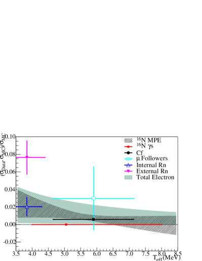
The MPE fit was also applied to the ⁸Li source but this was not included in the calculation due to the low statistics of the measurement. However, the energy dependence of both the ⁸Li and the ¹⁶N MPE fits were used to demonstrate that the use of a constant $\sigma_{\rm extra}$ across the energy spectrum was consistent with the data available.

VIII.3.2 Energy Resolution Uncertainties for Phase II Neutron Capture Events

The energy resolution for neutron capture events in Phase II was measured using the ²⁵²Cf source, with a verification performed using a ‘muon follower’ data set, consisting of neutron capture events occurring within a defined time window after a muon passed through the detector.

There are fewer uncertainties associated with the neutron measurement since the ²⁵²Cf source produced neutrons whose captures on ³⁵Cl and deuterium resulted in the same $\gamma$ cascades as those from NC events. The measurement was performed by numerically convolving a spline-fit of the Monte Carlo energy distribution with a Gaussian and fitting the resulting form to the data. The mean and width of the convolving Gaussian were allowed to vary, in order to take into account possible correlations between energy scale and resolution effects. The result was $\sigma_{\rm extra}=0.153\pm 0.018$ MeV. The observed energy scale from this measurement agreed very well with that evaluated in Sec. VIII.2.

The statistics of the muon follower data set were low, and the resulting uncertainty on the measurement was therefore relatively large. Nevertheless, a similar analysis was performed, giving a $\sigma_{\rm extra}$ of $0.237\pm 0.144$ MeV.

The weighted mean of the two points was used for the final correction to the energy resolution of neutron capture events in Phase II, with its associated uncertainty, with the value dominated by the ²⁵²Cf measurement: $\sigma_{\rm extra}=0.154\pm 0.018$ MeV. Both points are also shown on Fig. 10.

VIII.3.3 Energy Resolution Uncertainties for Phase I Electron-like Events

No radon spikes were deployed in Phase I, and so only the two ¹⁶N measurements were available. Both the MPE fit and the Gaussian convolution to the $\gamma$-ray energy distribution were performed for Phase I ¹⁶N runs, in the same manner as for Phase II (Sec. VIII.3.1). The central correction value was taken from the MPE fit directly, giving $\sigma_{\rm extra}=0.155\pm 0.036$ MeV. The small number of energy resolution measurements in Phase I provides fewer handles on the uncertainty than the much-better calibrated Phase II. The uncertainties in Phase I were therefore chosen to match those of Phase II. The width of the convolving Gaussian for Phase I events was therefore taken as $\sigma_{\rm extra}=0.155^{+0.041}_{-0.080}$ MeV. This was also applied to neutron capture events in Phase I, since the event topologies were similar.

VIII.4 Energy Linearity

The corrections derived in Sec. VIII.2 were done primarily using the ¹⁶N source, and therefore the uncertainty in the energy scale at the ¹⁶N energy is very small. An additional uncertainty was included to account for possible differential changes in the energy scale that were not correctly modeled in the Monte Carlo simulation. Such changes could be caused by residual crosstalk hits, or mis-modeling of the multi-photon PMT hit probabilities in the energy reconstruction algorithm. The differential changes were determined relative to the ¹⁶N point, and used calibration sources whose energies were substantially higher.

The pT source provided $\gamma$s roughly 14 MeV higher in energy than those from ¹⁶N, resulting in a good lever-arm on any non-linear effects. This source was only deployed in Phase I since deployment in Phase II would have resulted in an overwhelming neutron signal. The difference between data and Monte Carlo-reconstructed event energies was measured to be $-$1.36 $\pm$ 0.01% at the energy of the pT source.

The MPE fit described in Sec. VIII.2 was applied here to the ⁸Li source, including an additional term in the parameterization to model first-order differential changes in the energy scale. The fit was done to both data and Monte Carlo events, and a difference of just $-0.011\pm 0.004$% was found, evaluated at the same energy as the pT source $\gamma$ rays.

Giving the pT and ⁸Li sources equal weight, the average shift in energy scale at the energy of the pT source was found to be $-$0.69%. Using this as a measure of the degree by which the Monte Carlo energy scale could vary differentially from the data and assuming a linear interpolation between the ¹⁶N and pT energies, the linearity uncertainty was parameterized in terms of the difference of an event’s energy from the ¹⁶N source ($\sim$5.05 MeV). This results in a scaling factor that can be applied to the energy of each Monte Carlo event used to build the PDFs in the signal extraction procedure. Conservatively, this was applied as a two-sided uncertainty:

$$T^{\prime}_{\rm eff}=\left[1.0\pm 0.0069\times\left(\frac{T_{\rm eff}-5.05}{19.0-5.05}\right)\right]T_{\rm eff},$$ (9)

where 19 MeV is the effective energy of the pT source, $T_{\rm eff}$ is the original effective kinetic energy of an individual event and $T^{\prime}_{\rm eff}$ is the modified energy.

Tests using both the ⁸Li and ²⁵²Cf sources suggested no evidence for any linearity shift in Phase II. We expect any source of linearity shift to be common across the two phases, however, and therefore the results from Phase I were conservatively taken to apply to both phases in a correlated fashion.

IX Event Isotropy

As discussed in Sec. II, we used a measure of event ‘isotropy’ as one dimension of our PDFs to help distinguish different types of events. By ‘isotropy’ we mean the degree of uniformity in solid angle of the hit PMTs relative to the fitted event location.

Single electron events, like those created in neutrino CC and ES reactions, had a Cherenkov cone that, at solar neutrino energies, was somewhat diffuse due to electron multiple scattering in the water. Nevertheless, even with the multiple scattering, these events were characterized by a fairly tight cluster of PMT hits in a cone aligned with the forward direction of the electron.

Neutron capture events on deuterium in Phase I led to a single 6.25 MeV $\gamma$ ray. Although these events could produce multiple Compton electrons and, hence, a number of Cherenkov cones that distributed hits more widely than single electrons, Phase I neutron capture events in the data set were dominated by single Compton scatters and, thus, isotropy was not useful in distinguishing them from CC or ES events.

In contrast, in Phase II neutrons captured primarily on ³⁵Cl, which typically led to a $\gamma$ cascade that looks very different from single electrons. Neutron capture on ³⁵Cl typically produced several $\gamma$ rays, with energies totaling $8.6$ MeV, which distributed PMT hits more uniformly in solid angle. The isotropy distribution for these events is thus a convolution of the isotropy distribution of single $\gamma$-ray events with the directional distribution of the $\gamma$ rays emitted in the possible $\gamma$-decay cascades.

The isotropy of background events can also be significantly different from that of single electron and neutron events. Decays of ²⁰⁸Tl, for example, produce both a $\beta$ and a 2.614 MeV $\gamma$ ray and, thus, resulted in a different distribution of hit PMTs than either single electrons or single $\gamma$s.

The measure of isotropy was therefore critical to the analysis, helping us to separate CC and ES events from NC events, and both of these from low-energy background events.

We examined several measures of isotropy, including a full correlation function, the average angle between all possible pairwise combinations of hit PMTs, and constructions of several variables using Fisher discriminants. We found that, for the most part, they all had comparable separation power between the single electron (CC and ES) and the neutron (NC) signals. As in our previous Phase II publications nsp , we opted to use a linear combination of parameters, $\beta_{14}\equiv\beta_{1}+4\beta_{4}$, where:

$$\beta_{l}=\frac{2}{N(N-1)}\sum_{i=1}^{N-1}\sum_{j=i+1}^{N}P_{l}(\cos\theta_{ij}).$$ (10)

In this expression, $P_{l}$ is the Legendre polynomial of order $l$, $\theta_{ij}$ is the angle between triggered PMTs $i$ and $j$ relative to the reconstructed event vertex, and $N$ is the total number of triggered PMTs in the event. Very isotropic events have low (even negative) values of $\beta_{14}$.

IX.1 Uncertainties on the Isotropy Measure

We parameterized the difference between the predicted $\beta_{14}$ PDF and the true PDF by a fractional shift in the mean, $\bar{\beta}_{14}$, and a broadening of the width, $\sigma_{\beta_{14}}$. We also allowed for an energy dependence in the shifts.

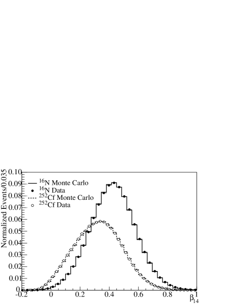
Figure 11 shows $\beta_{14}$ distributions of Phase II data from ²⁵²Cf and $\rm{}^{16}{N}$ sources and from corresponding MC simulations. The $\rm{}^{16}{N}$ source emitted a single 6.13 MeV $\gamma$ ray, which usually underwent Compton scattering and produced one or more electron tracks, while neutrons from the ²⁵²Cf source were typically captured in Phase II by the chlorine additive, leading to a cascade of several $\gamma$ rays. It is clear from the figure that the $\rm{}^{16}{N}$ data and Monte Carlo agree very well, while the Monte Carlo simulation of the ²⁵²Cf source shows a very small shift toward higher $\beta_{14}$ values (less isotropic events than in the data). This shift is discussed in Sec. IX.1.3.

Figure 11: $\beta_{14}$ isotropy distributions for ²⁵²Cf data and MC and $\rm{}^{16}{N}$ data and MC. There is a very small shift of the Monte Carlo ²⁵²Cf $\beta_{14}$ distribution toward higher (less isotropic) values.

Errors in the simulated distributions of $\beta_{14}$ can have several sources: incorrect modeling of the detector optics or photomultiplier tubes, unmodeled event vertex reconstruction errors, errors in the model of the production of Cherenkov light (including the interactions of $\gamma$ rays and electrons in the detector) and, for neutrons captured on ³⁵Cl, uncertainties in our knowledge of the $\gamma$ cascade sequences and correlations between the directions of the multiple $\gamma$ rays.

Except for the last item, these errors affect all event types. For Phase I, in which neutrons were captured on deuterons, we allowed for correlations among the uncertainties on all signals and most backgrounds. For Phase II, we treated the uncertainties on the mean and width of the $\beta_{14}$ distribution for NC events and photodisintegration neutrons separately from the other event types. Uncertainties on the $\beta_{14}$ distributions of $\beta$s and $\gamma$s from radioactive background events were treated the same as for CC and ES events. The one exception to this was PMT $\beta$-$\gamma$ events, whose location at the PMT array led to effects on the $\beta_{14}$ distribution that are not present in the other signals. The $\beta_{14}$ distribution and associated uncertainties for PMT $\beta$-$\gamma$s are discussed in Sec. XIII.3.

As usual in this analysis, we derived uncertainties on the mean, width, and energy dependence of the $\beta_{14}$ distribution by comparing calibration source data to Monte Carlo simulations of the calibration source runs. When we found a difference that was corroborated by more than one source, or was caused by known errors in the simulation, we adjusted the simulated distribution by shifting the mean of the distribution and/or convolving the distribution with a smearing function to better match the calibration data. In such cases, additional uncertainties associated with the correction were included.

IX.1.1 $\beta_{14}$ Uncertainties for Phase II Electron-like Events

The primary measure of isotropy uncertainties for Phase II electron-like events comes from comparisons of ¹⁶N calibration source data to Monte Carlo simulation. We fit Gaussians to both the data and simulated events for each run, and calculated the fractional difference between the fitted parameters. Figure 12 shows the fractional difference in the means as a function of $R^{3}$. Each point shown is the fractional difference for a single run, with the error bar evaluated as the combination of the uncertainty on the fit parameters for data and Monte Carlo events. The detector region in which the source was deployed has been identified for each run.

Also shown in Fig. 12 are the averages of these differences, in several radial bins.

Figure 12: (Color online) Fractional differences in the mean of the $\beta_{14}$ distributions for data and Monte Carlo, for the Phase II ¹⁶N calibration source. Also shown in the figure are the averages in each radial bin, with the bands indicating the volume-weighted uncertainty in each bin.

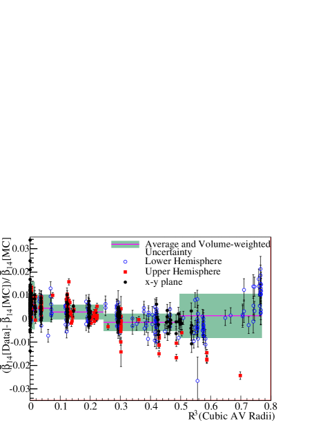
The uncertainty on each average is the standard deviation of the points in that bin, weighted by the volume represented by the bin (smaller volumes have larger uncertainties). The overall weighted average within the entire 550 cm radius fiducial volume is consistent with zero, with an uncertainty of $\pm 0.21$%. The calibration data were collected at a high rate relative to normal neutrino data runs and, so, we added to this an uncertainty to account for the difference in $\beta_{14}$ between high rate and low rate data ($\pm 0.1$%) by comparing low-rate and high-rate ¹⁶N source runs, as well as a small uncertainty of $\pm 0.002$% associated with a possible un-modeled time-dependence obtained by comparing data and Monte Carlo differences over time. The quadrature combination of these uncertainties on the mean of the $\beta_{14}$ distribution totals $\pm 0.24$%. A similar analysis was performed for the width of the $\beta_{14}$ distribution, yielding a total fractional uncertainty of $\pm 0.54$%.

IX.1.2 $\beta_{14}$ Uncertainties for Phase I Electron-like Events

We applied an identical analysis to the Phase I ¹⁶N data but, as shown in Figure 13, we found a difference of $-0.81\pm 0.20$% between the means of the $\beta_{14}$ distributions for source data and source simulations. Comparison of ¹⁶N data between Phase I and Phase II showed them to be consistent, and the (data-Monte Carlo) difference seen in Fig. 13 to be due to a shift in the simulated events. Further investigation showed that the difference was caused by the value of the Rayleigh scattering length used in the Phase I simulation. Explicit measurements of the Rayleigh scattering had been made and used in the simulation for Phase II but no such measurements existed for Phase I. Use of the Phase II Rayleigh scattering length in Phase I simulations was found to produce the desired magnitude of shift, and we therefore corrected the $\beta_{14}$ values of all simulated Phase I events by a factor of $(1-0.0081)=0.9919$.

Figure 13: (Color online) Fractional differences in the mean of the $\beta_{14}$ distributions for data and Monte Carlo, for the Phase I ¹⁶N calibration source. Also shown in the figure are the averages in each radial bin, with the bands indicating the volume-weighted uncertainty in each bin.

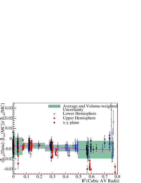
We included three uncertainties associated with this correction. The first was 0.20% on the correction itself, evaluated from the volume-weighted average of the data and Monte Carlo differences for Phase I, as shown in Fig. 13. To take into account the fact that we used the consistency in the ¹⁶N data between the two phases to support the correction of $-0.81$%, we added in quadrature the uncertainty on the difference between the means of the Phase  I and Phase II ¹⁶N $\beta_{14}$ distributions, which was 0.34%. Finally, because we used the consistency of the Phase II data with the Monte Carlo simulation as evidence that the Phase I $\beta_{14}$ distribution was correct, aside from the Rayleigh scattering correction, we included the volume-weighted Phase II uncertainty on the offset of the mean (0.21% from Fig. 12 in Sec. IX.1.1).

The evaluations of the uncertainties associated with rate dependence and time dependence in Phase I were 0.08% and 0.03%, respectively, and the overall uncertainty on the mean of the $\beta_{14}$ distribution in Phase I thus totaled 0.42%.

We evaluated the uncertainty on the width of the $\beta_{14}$ distribution for Phase I in the same way as for Phase II, finding a fractional uncertainty which also totaled 0.42%.

IX.1.3 $\beta_{14}$ Uncertainties for Phase II Neutron Capture Events

Neutron capture events in Phase II were distinct from other neutrino-induced events and backgrounds in that the $\gamma$ cascade was more isotropic than a single electron or $\gamma$ ray. The primary measurement of the uncertainty on the mean of the $\beta_{14}$ distribution comes from deployments of the ²⁵²Cf source, which produced several neutrons per fission decay. The $\beta_{14}$ distribution of the resulting neutron capture events was noticeably non-Gaussian, and we therefore derived uncertainties on the mean and width by fitting the $\beta_{14}$ distributions from simulated ²⁵²Cf runs directly to the distributions of data. The fit allowed for scaling as well as convolution with a Gaussian smearing function. Figure 14 shows the fit of a simulated ²⁵²Cf run to data, in which the fitted scaling was -1.2% and the smearing was an additional 1.8% of the width of the Monte Carlo distribution.

Figure 14: (Color online) Fit of Monte Carlo simulated $\beta_{14}$ distribution for neutron capture events from ²⁵²Cf to data taken with the ²⁵²Cf source. The fitted shift for this sample is $-$1.2%, and the additional smear is 1.8%, before any corrections for bias.

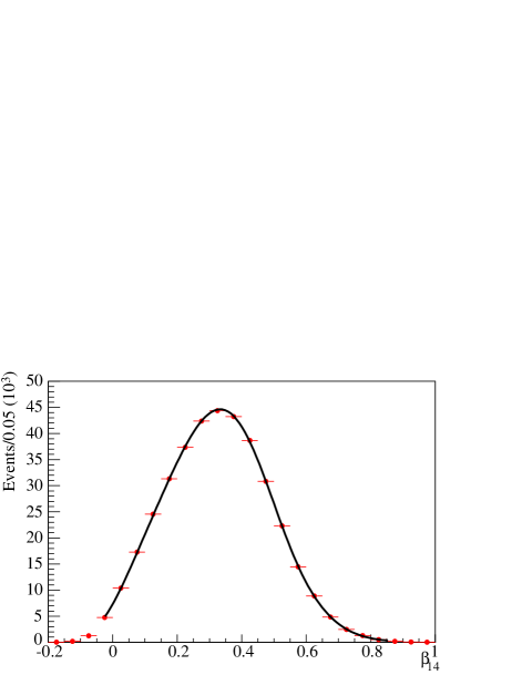
We derived scaling factors from fits like that in Fig. 14 for all ²⁵²Cf runs, and then volume-weighted them in the same way as for the ¹⁶N data. The average of the volume-weighted differences showed an overall offset between the means of the $\beta_{14}$ distributions for data and Monte Carlo of $\sim-1.4$%. This result was not consistent with that from the ¹⁶N data for Phase II (which, as discussed above, had no significant offset), which indicated that the shift was not due to a detector effect. To check whether the shift was caused by mis-modeling of the ²⁵²Cf source in the simulation, we performed the same analysis on several types of neutron capture events: neutrons produced by passage of a muon through the detector (‘muon followers’), neutrons from a tagged Am-Be source, and neutrons produced by deuteron photodisintegration during the deployment of a radon spike in the detector. Figure 15 shows results from these sources. An energy-dependent fit to all sources except ²⁵²Cf showed an offset of $-1.12\pm 0.31$%, consistent with the data from the ²⁵²Cf source. This indicated that the offset was likely not a source effect but was instead associated with the simulation of the $\gamma$ cascade from neutron captures on chlorine, possibly with some contribution from the energy-dependent correction of the Monte Carlo value for $\beta_{14}$ presented in Sec. IX.1.5. All sources taken together gave an overall offset of $-1.44$%, and we therefore corrected the $\beta_{14}$ PDF by multiplying each simulated event’s $\beta_{14}$ value by $(1+\delta_{\beta_{14}})=(1-0.0144)=0.9856$.

Figure 15: (Color online) Fractional difference in mean $\beta_{14}$ between data and Monte Carlo events for several neutron sources. The horizontal band indicates the error on the overall $-$1.44% correction.

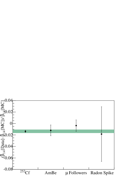
The uncertainties on this correction came first from the uncertainty on the overall average, which was 0.17%. To this we added in quadrature the same rate- and time-dependent uncertainties as were calculated for the Phase II ¹⁶N sources. We also added an uncertainty associated with the multiplicity of neutrons from the ²⁵²Cf source of 0.09% (neutrons produced by either photodisintegration of deuterons or the NC reaction are singles, whereas the ²⁵²Cf source produces multiple neutrons/decay), and 0.03% uncertainty to account for the relatively sparse sampling of the detector, giving a total of 0.22%. Conservatively, we included a further uncertainty based on the difference between ²⁵²Cf and the other neutron-source data, a one-sided uncertainty of 0.31%. The total uncertainty on the mean of the $\beta_{14}$ distribution for Phase II neutron captures was therefore ${}^{+0.38}_{-0.22}$%.

As well as a measure of any required shift, the fit described above also allowed for the widths of the data and Monte Carlo distributions to differ. A resolution parameter was varied in the fit, as the standard deviation of the Gaussian by which the Monte Carlo distribution was analytically convolved. The results for each ²⁵²Cf run were volume-weighted using the procedure described above to result in an average overall smearing value. The same fit was performed on a sample of Monte Carlo-generated data, and the bias determined from these fits was subtracted from the overall average. The result was a fractional smearing correction to be applied to the PDFs of 0.43%, with an uncertainty (including all sources described above: time, rate, multiplicity, and sampling) of 0.31%.

IX.1.4 $\beta_{14}$ Uncertainties for Phase I Neutron Capture Events

Neutrons created in Phase I captured on deuterons, releasing a single 6.25 MeV $\gamma$ ray. The uncertainties on the mean and width of the $\beta_{14}$ distribution were therefore well-estimated by the measurements made with the ¹⁶N 6.13 MeV $\gamma$-ray source, already discussed in Sec. IX.1.2. We therefore used the same uncertainties for both event types, applied in a correlated fashion.

IX.1.5 Energy Dependence of $\beta_{14}$ Uncertainties

A final systematic uncertainty on the $\beta_{14}$ distributions is their energy dependence. In Figure 16 we show the energy

Figure 16: (Color online) Fractional shift in mean $\beta_{14}$ between data and Monte Carlo simulation in Phase II for several calibration sources as a function of kinetic energy, with the fit to Eq. (11) shown.

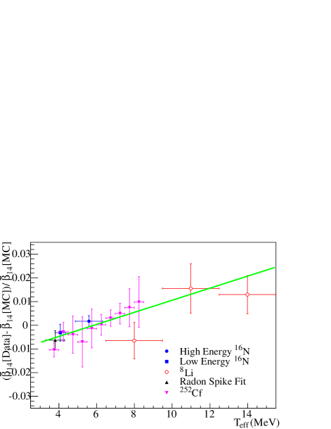
dependence of the fractional difference between Monte Carlo predictions of the mean of the $\beta_{14}$ distribution and data from several different sources: the Phase II radon spike, low and high energy ¹⁶N source events, the ²⁵²Cf source (with the data corrected by the 1.44% shift discussed above), and ⁸Li-source $\beta$ events in three energy bins. There clearly is an energy dependence in the data, which we fit with a function of the form:

$$f=\delta_{\beta_{14}}+m_{\beta_{14}}(T_{\rm eff}-5.6\rm~{}MeV),$$ (11)

where $T_{\rm eff}$ is kinetic energy, and 5.6 MeV is the kinetic energy at the high-energy ¹⁶N point (the point used to determine the offset in the mean of the Phase II electron $\beta_{14}$ distribution). With this parameterization, the offset ($\delta_{\beta_{14}}$) and the slope ($m_{\beta_{14}}$) are uncorrelated. Given that all the sources exhibited the same trend, we applied the same slope to all event types, but used the different offsets and uncertainties for $\delta_{\beta_{14}}$ described in the previous sections. We performed a similar analysis for Phase I, although less calibration data were available, and found that the same slope fit the ¹⁶N and ⁸Li data in this phase.

We found no energy dependence in the broadening of the width of the $\beta_{14}$ distributions. These uncertainties were therefore treated as independent of energy.

The corrections and uncertainties to the $\beta_{14}$ distributions are listed in Tables 4 and 5.

Phase/Particles	$\delta_{\beta_{14}}$	$m_{\beta_{14}}$ (10-3 MeV-1)
II/electrons	0.0$\,\pm\,$0.0024	2.76$\,\pm\,0.696$
II/neutrons	$-0.0144\,^{+0.0038}_{-0.0022}$	2.76$\,\pm\,0.696$
I/electrons	$-$0.0081$\,\pm\,$0.0042	2.76$\,\pm\,0.696$
I/neutrons	$-$0.0081$\,\pm\,$0.0042	2.76$\,\pm\,0.696$

Table 4: Summary of uncertainties on the $\beta_{14}$ scale. The $\beta_{14}$ of each event was corrected by: $\beta_{14}\rightarrow\beta_{14}(1+(\delta_{\beta_{14}}+m_{\beta_{14}}(T_{\rm eff}-5.6{\rm~{}MeV})))$.

Phase/Particles	Correction (%)	Uncertainty (%)
II/electrons	0.0	$\pm\,$0.42
II/neutrons	0.43	$\pm\,$0.31
I/electrons	0.0	$\pm\,$0.42
I/neutrons	0.0	$\pm\,$0.42

Table 5: Summary of uncertainties on the $\beta_{14}$ width.

X Cuts and Efficiencies

The data set contains two main types of background events: physics backgrounds, due to radioactive decays, and instrumental backgrounds, caused by the detector itself. Two sets of cuts were developed to remove these events, described in Sections X.1 and X.2. Each set of cuts had an associated level of signal loss, which was taken into account in the measurement of neutrino flux and spectra as described in Sec. X.5.

X.1 Low-Level (Instrumental) Cuts

There were many sources of instrumentally-generated events in the SNO detector, which produced hits originating either in the PMTs or in the electronics channels. Static discharges in the nitrogen in the neck of the acrylic vessel and ‘flasher’ PMTs, in which discharges occurred within a photomultiplier tube itself, produced light in the detector. Electronic pickup generated by noise on the deck above the detector or by high-voltage breakdown could produce hits in electronics channels. We removed these instrumental backgrounds with a suite of loose ‘low-level’ cuts that rejected events before event reconstruction. The cuts were based on event characteristics such as the distribution of PMT hit times, the presence of unusually low or high PMT charges, or unusual time correlations between events (such as bursts of events with large numbers of hits). More details on these low-level cuts can be found in longd2o ; nsp . We used the same cuts and cut criteria here, with the exception that the simple burst cut used in longd2o was not used in this analysis because it was redundant with other burst cuts.

The acceptance of these cuts was re-evaluated for this analysis, particularly in the low-threshold region (below $T_{\rm eff}=5.0$ MeV) where the cuts had not previously been examined in detail. We discuss the results of these cut acceptance measurements in Sec. X.5.1.

X.2 High-Level Cuts

Background radioactivity events were produced primarily by the decays of ²¹⁴Bi and ²⁰⁸Tl. Lower energy ($T_{\rm eff}<3$ MeV) decays of these nuclei in the heavy water could appear above our $T_{\rm eff}=3.5$ MeV threshold because of the broad energy resolution intrinsic to a Cherenkov detector. Decays within the walls of the acrylic vessel, the light water surrounding the vessel, and the photomultiplier tube array could pass the energy cut and have misreconstructed vertex positions which falsely placed them within the fiducial volume. The PMT array was, by far, the radioactively hottest component of the SNO detector and, consequently, the largest source of background events. We designed a suite of 13 loose cuts that used ‘high-level’ information (reconstructed event position, direction, and energy) to remove events whose likely origin was either outside the fiducial volume or whose true energy was below our threshold. All of the cuts were adjusted based exclusively on simulated events and calibration data. Several of the cuts had a high degree of redundancy in order to maximize background rejection. The acceptance of the cuts was therefore evaluated collectively, as described in Sec. X.5.

Five of the high-level cuts removed backgrounds using Kolmogorov-Smirnov (KS) tests of the hypothesis that the event had a single Cherenkov-electron track. Two of these tests compared azimuthal and two-dimensional (polar vs azimuthal) angular distributions to those expected for Cherenkov light produced by an electron, and two others did the same for hits restricted to a narrow prompt time window. The fifth of these KS tests was a comparison of the distribution of fitted PMT time residuals (see Eq. (2)) with the expected distribution for direct Cherenkov light.

Three more of the cuts applied event ‘isotropy’ to remove misreconstructed events. Events whose true origins were well outside the fiducial volume but which reconstructed inside tend to appear very anisotropic. For one of these cuts we used the mean angle between pairs of PMTs, ($\theta_{ij}$), and for another the isotropy parameter $\beta_{14}$, which is described in Sec. IX. Both of these have been used in previous SNO analyses longd2o ; nsp . The third of these cuts was based on the charge-weighted mean pair angle, $\theta_{ij}$, in which each pair angle is weighted by the product of the detected charges of the two PMTs in the pair.

Further cuts used information from the energy reconstruction algorithm discussed in Sec. VIII.1. Two cuts removed events whose reported energy uncertainty was well outside of the range expected from the known energy resolution. These are referred to in Sections X.5.3–X.5.5 as the ‘energy-uncertainty’ cuts. The third was a comparison of the energy estimated with FTK (which used all hits) with that from a prompt-light-only energy estimator. Events whose origins were outside the acrylic vessel and which pointed outward often had a larger fraction of prompt hits because the direct light was not attenuated by the acrylic vessel. Such an event would have a higher energy as measured by a prompt-light energy estimator than by the total-light energy reconstruction of FTK. We normalized the ratio of these two energy estimates by the ratio of prompt to total hits in the event. The cut itself was two-dimensional: events were removed if the normalized ratio of energy estimates was unusually large and the charge-weighted $\theta_{ij}$ was unusually low (the latter indicating an outward-pointing event with a tight cluster of hits).

The last two high-level cuts were also used in determining the PDFs for radioactive backgrounds from the PMTs. The first of these, the in-time ratio (ITR) cut, removed events based on the ratio of the prompt hits to the total hits. The prompt time window for the ITR cut extended from 2.5 ns before the reconstructed event time to 5.0 ns after, and the full-event window was roughly 250 ns long. The mean of the ITR distribution for SNO events is at 0.74. Events that were reconstructed at positions far from their true origin tend to have small ITR values, because the PMT hits were spread across the entire time window. In previous analyses longd2o ; nsp ; snoncd we used the ITR cut with a fixed threshold, rejecting events with an in-time ratio smaller than 0.55. For the lower-energy events included in this analysis, the lower number of hits caused the distribution of ITR to broaden and introduced a large, energy-dependent bias in the acceptance of the cut. We therefore changed the cut threshold to scale with the number of hits ($N_{\rm hit}$) in an event. The fixed value of 0.55 used in earlier publications corresponded to cutting events that fell more than 2.7$\sigma$ below the mean of the distribution, and we retained this criterion, so that the new version of the ITR cut rejected events that were more than 2.7$\sigma$ below the mean of 0.74, where now $\sigma=0.43/\sqrt{N_{\rm hit}}$.

The last cut was aimed directly at removing events produced by radioactive decays in the PMTs themselves. Such events produced light either in the PMT glass or in the light water, just in front of the PMTs. Although only a tiny fraction of such events were misreconstructed inside the fiducial volume, the PMT array was relatively hot, with a total decay rate from uranium and thorium chain daughters of a few kHz. Because of their origin within or near the PMTs, these events were characterized by a large charge in one PMT (or distributed over a few nearby PMTs) with hit times that preceded the reconstructed event time. The ‘early charge’ (EQ) cut therefore examined PMT hits in a window that ran from $-$75 ns to $-$25 ns before the event time. If a PMT hit in this window had an unusually high charge, or there was an unusually large number of hits in this window, then the event was cut. To account for variations in PMT gain, ‘unusually high charge’ was defined by using the known charge spectrum of the PMT in question to calculate the probability of observing a charge as high as observed or higher. If more than one hit was in the window, a trials penalty was imposed on the tube with the lowest probability, and an event was cut if this trials-corrected probability was smaller than 0.01. We defined ‘unusually large number of hits’ in a similar way, by comparing the number of hits observed in the early time window to the expected number, given the total number of hits in the event. If the Poisson probability of having the observed number in the early time window was below 0.002, the event was cut.

X.3 Burst Removal

Atmospheric neutrinos, spontaneous fission, and cosmic-ray muons could all produce bursts of events that were clearly not due to solar neutrinos. Most of these bursts had a detectable primary event (like a high-energy atmospheric-neutrino event) followed by several neutron events. In addition, many instrumentally-generated events came in bursts, such as those associated with high-voltage breakdown in a PMT.

We therefore applied several cuts to the data set to remove most of these time-correlated events. Four of these were part of the suite of instrumental cuts described in Sec. X.1. The first removed events that were within 5 $\mu$s of a previous event and, therefore, eliminated events associated with PMT afterpulsing or Michel electrons from decays of stopped muons. The second removed all events within 20 seconds of an event that had been tagged as a muon. Most of these ‘muon followers’ were neutrons created by passage of a cosmic-ray muon through the heavy water, which captured either on deuterons or, in Phase II, on ³⁵Cl, but the cut also removed longer-lived cosmogenic activity. The muon follower cut resulted in a very small additional overall detector deadtime because of the very low rate of cosmic rays at SNO’s depth. Atmospheric neutrinos could also produce neutrons, either directly or by creating muons which, in turn, disintegrated deuterons. We therefore removed any event within 250 ms of a previous event that had $N_{\rm hit}>60$ (Phase I) or $N_{\rm hit}>150$ (Phase II). The fourth cut was aimed primarily at residual instrumental bursts, and removed events that were part of a set of six or more with $N_{\rm hit}>40$ that occurred within an interval of six seconds.

Because of the relatively loose criteria used, after these cuts were applied there were still time-correlated events in the SNO data set that were very unlikely to be solar neutrinos, but were primarily low-multiplicity neutrons created by atmospheric neutrino interactions. We therefore applied a final ‘coincidence cut’ that removed events if two or more occurred within a few neutron capture times of each other. For Phase I this window was 100 ms; a shorter window of 15 ms was used for Phase II because of the shorter neutron capture time on chlorine compared to deuterium. The cut was ‘retriggerable’, in that the window was extended for its full length past the last event found. If a new event was thus ‘caught’, the window was again extended. We calculated that this cut removed less than one pair of events from each data set due to accidental coincidences.

X.4 Cut Summary

The numbers of events in the data sets after successive application of each set of cuts are shown in Table 6. The burst cuts described in Sec. X.3 are included in instrumental cuts, except for the final coincidence cut, which appears in the last line of the table.

Events	Phase I	Phase II
Full data set	128421119	115068751
Instrumental	115328384	102079435
Reconstruction	92159034	77661692
Fiducial volume ($<$550 cm)	11491488	8897178
Energy range (3.5–20 MeV)	25570	40070
High-level cuts	9346	18285
Coincidence cut	9337	18228

Table 6: Number of events remaining in the data set after successive application of each set of cuts.

X.5 Cut Acceptance

As in previous analyses longd2o , the fraction of signal events expected to pass the full set of analysis cuts (the ‘cut acceptance’) was determined by separating the cuts into three groups: instrumental, reconstruction, and high-level cuts. Correlations between these groups had been shown to be minimal nsp , and it was verified that this was still true after the addition of new high-level cuts for this analysis.

The ¹⁶N and ⁸Li calibration sources were used for the primary measurements of cut acceptance and the ²⁵²Cf source was used for neutron capture events in Phase II. Neutron events in Phase I are well-modeled by ¹⁶N events since capture on deuterium resulted in a single $\gamma$ at 6.25 MeV and ¹⁶N was a source of 6.13 MeV $\gamma$s.

X.5.1 Instrumental Cut Acceptance

The instrumental cuts were not simulated in the Monte Carlo code and, therefore, we could not make a relative estimate of their acceptance by comparing simulation to data. Instead, an absolute measure of their acceptance was made using calibration data and applied as a correction (with uncertainties) to the PDFs.

Being a near-perfect source of CC-like electron events, the ⁸Li source was used to evaluate the signal loss for electron-like events, and ²⁵²Cf was used for Phase II neutron capture events. The ¹⁶N source was used as a check and any difference in the values obtained was conservatively taken as a two-sided systematic uncertainty. Figure 17 shows the ¹⁶N and ⁸Li measurements in Phase I. The weighted mean of the ⁸Li signal loss shown in the figure was taken as the correction to the PDFs, and the median deviation of the points from this value was used to represent the energy-dependent uncertainty.

Figure 17: (Color online) Signal loss due to the instrumental cuts for the ¹⁶N and ⁸Li calibration sources as a function of reconstructed kinetic energy, in Phase I.

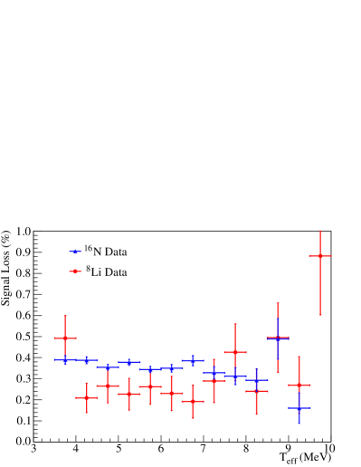
The ¹⁶N source, which was deployed more frequently and at more positions than ⁸Li, was used to determine time- and position-dependent uncertainties. Runs were binned by position and date, and the median deviation of the bin values from the best-fit value was taken as the measure of systematic uncertainty.

After combination of the systematic uncertainties in quadrature, the final estimates of signal loss due to the instrumental cuts were:

• Phase I: $0.214$% $\pm 0.026$ (stat) $\pm 0.094$ (syst)

• Phase II $e^{-}$: $0.291$% $\pm 0.028$ (stat) $\pm 0.202$ (syst)

• Phase II $n$: $0.303$% $\pm 0.003$ (stat) $\pm 0.186$ (syst)

where “$e^{-}$” refers to electron-like events and “$n$” to neutron captures. The acceptance is given by one minus the fractional signal loss and was applied as an adjustment to the normalization of the PDFs.

X.5.2 Acceptance of Reconstruction

Occasionally, the reconstruction algorithm failed to converge, and returned no vertex for an event. In past analyses, an upper bound was placed on the resulting signal loss, by using calibration source data, but a different approach was used in this analysis. What is important is how well the effect is reproduced in the simulation. Therefore, a comparison was made of the acceptance of data and Monte Carlo events and the difference of the ratio from unity was taken as a systematic uncertainty on the PDF normalization.

Results from the ¹⁶N source, and the ²⁵²Cf source for Phase II neutrons, demonstrated that the signal loss in the data was reproduced by the simulation to within the statistical uncertainties. Analysis of runs taken during the two phases showed no significant deviation with time. A position-dependent uncertainty was evaluated by taking the ratio of the acceptance of ¹⁶N data and Monte Carlo events as a function of source deployment position. The difference of the weighted average of the points from 1.0 was taken as the value of the uncertainty. The ⁸Li source was used to investigate energy dependence. As expected, the signal loss decreased at higher energies, where more information was available to reconstruct an event. The simulation was shown to reproduce this effect very accurately and the uncertainty was therefore treated in the same manner as the position-dependent uncertainty.

Combining the systematic uncertainties in quadrature, we obtained the final uncertainties associated with reconstruction acceptance:

• Phase I: $\pm 0.034\%$ (stat) $\pm 0.060\%$ (syst)

• Phase II $e^{-}$: $\pm 0.037\%$ (stat) $\pm 0.090\%$ (syst)

• Phase II $n$: $\pm 0.000\%$ (stat) $\pm 0.009\%$ (syst)

X.5.3 High-Level Cut Acceptance

To take into account the acceptance of the high-level cuts, the ratio of the cut acceptance for data and Monte Carlo events was calculated and applied to the PDFs as a normalization correction. This ratio was evaluated as a function of energy, position and time.

The energy-uncertainty cuts described in Sec. X.2 were observed to have much stronger variations in signal loss as a function of position and energy than the other high-level cuts and were therefore treated separately. It was verified that the correlations between the two resulting subsets of high-level cuts were minimal, so that treating them independently was a valid approach. The following sections describe the analysis for each subset of cuts, where ‘reduced high-level cuts’ refers to the subset that does not include the energy-uncertainty cuts.

X.5.4 Reduced High-Level Cut Acceptance

The data/Monte Carlo acceptance ratio and its uncertainty were calculated for each calibration source run. The runs were divided into radial bins, and the error-weighted mean and standard deviation were calculated in each bin. Finally, the volume-weighted average of the bin values was calculated.

The energy dependence of the acceptance ratio was investigated using ¹⁶N and ⁸Li data for electron-like events and ²⁵²Cf for Phase II neutron capture events. The ¹⁶N data were restricted to the energies below 9 MeV to avoid complications associated with event pile-up caused by the high rate of the calibration source.

The measurements from ¹⁶N and ⁸Li were in very good agreement, and were both consistent with the acceptance ratio having no dependence on energy. The normalization correction for the PDFs was therefore evaluated using the ¹⁶N source data by taking the weighted mean of the values in each energy bin. The median deviation of the ⁸Li points from the best-fit was taken as a systematic uncertainty on the energy-dependence.

The acceptance ratio for Phase II neutron capture events was evaluated using ²⁵²Cf data. To avoid pile-up of fission $\gamma$s, the events were required to have energies in the interval 4.5-9.5 MeV. An energy-dependent uncertainty was included to account for any variation of individual energy bins from the overall average.

The stability of the acceptance as a function of time was studied using ¹⁶N runs taken in the center of the detector. No trend was observed, but the time variability was incorporated as an additional systematic uncertainty.

The ¹⁶N source was also used to evaluate a systematic uncertainty associated with a possible position dependence of the acceptance ratio. Runs were binned by position in the detector, the volume-weighted average of the bins was found and the mean deviation of the ratio in each bin from this value was calculated. A comparison of ¹⁶N and ²⁵²Cf source data showed that they exhibited statistically equivalent position dependences, so the more widely deployed ¹⁶N source was used to quantify this effect for both electron-like and neutron capture events.

The acceptance corrections and associated uncertainties derived from the difference between the high-level cut acceptances for data and Monte Carlo events are summarized in Table 7.

	Phase I	Phase II $e^{-}$	Phase II $n$
Correction	0.9945	0.9958	0.9983
Stat uncert (%)	0.0273	0.0159	0.0196
Energy dep (%)	0.1897	0.1226	0.0005–2.3565
Position dep (%)	0.1630	0.3144	0.3144
Time dep (%)	0.0805	0.0130	0.0130

Table 7: Correction and associated uncertainties for the high-level cut acceptance ratio. The Phase II neutron energy-dependent uncertainty was treated differentially with energy; the quoted range covers the value across the energy spectrum.

X.5.5 Energy-Uncertainty Cut Acceptance

We expect that the effect of placing cuts on the uncertainty on the estimate of an event’s energy reported by the energy reconstruction algorithm should be the same for data and Monte Carlo events. Nevertheless, uncertainties on this assumption were evaluated using the ¹⁶N and ²⁵²Cf source data, applying the same energy ranges as in the reduced high-level cut analysis (Sec. X.5.4).

Differential uncertainties were evaluated using the same method as for the reduced high-level cuts. The stability over time was measured using ¹⁶N data. The acceptance ratio was observed to be stable, but an additional uncertainty was included based on the spread of the points.

The ¹⁶N and ²⁵²Cf data showed statistically equivalent position-dependent behavior in the acceptance of the energy-uncertainty cuts, and we therefore evaluated position-dependent uncertainties using the more widely-deployed ¹⁶N source. ¹⁶N source data were divided into 50 cm slices along the $z$-axis, and the acceptance ratios calculated in the slices were combined in a volume-weighted average. The uncertainty on this average was derived from the deviation of the points from unity.

The energy-uncertainty cuts were even more sensitive to the effects of pile-up than were the other high-level cuts. Therefore, to evaluate an energy-dependent uncertainty on the acceptance ratio for electron-like events, events from the ¹⁶N source were restricted to energies below 7 MeV, and the lower rate ⁸Li source was used for measurements at higher energies. ²⁵²Cf data were used for Phase II neutron capture events, with the deviations from unity measured in the 8.5–9 MeV bin also applied to higher energy events. This resulted in energy-dependent uncertainties for both electron-like and neutron capture events.

The uncertainties in acceptance were applied as uncertainties in normalization of the PDFs. The values are summarized in Table 8.

	Phase I	Phase II $e^{-}$	Phase II $n$
Stat uncert (%)	0.0377	0.0668	0.0322
Position dep (+) (%)	+0.0750	+0.0838	+0.0838
Position dep ($-$) (%)	$-$1.0760	$-$0.9897	$-$0.9897
Time dep (%)	0.0834	0.0531	0.0531

Table 8: Uncertainties on the energy-uncertainty cut acceptance ratio. Energy-dependent uncertainties were treated differentially with energy and are not shown. The uncertainty in position is asymmetric.

X.5.6 Overall Cut Acceptance

The final correction to the PDF normalization comes from combination of the high-level cut correction (Table 7) and the instrumental cut correction (Sec. X.5.1). The various contributions to uncertainty on signal loss were treated as uncorrelated and combined in quadrature to give the final uncertainty on the cut acceptance correction. Table 9 lists the final corrections and uncertainties.

	Phase I	Phase II $e^{-}$	Phase II $n$
Correction	0.9924	0.9930	0.9954
Pos uncertainty (%)	0.34–0.45	0.41–0.80	0.38–2.70
Neg uncertainty (%)	1.12–1.17	1.07–1.08	1.06–1.65

Table 9: Corrections applied to the Monte Carlo-generated PDFs due to cut acceptance. The uncertainties were evaluated differentially with energy; the quoted range covers their values across the energy spectrum.

Figure 18 shows a comparison of the cut acceptance for data and Monte Carlo events from a single ²⁵²Cf run in Phase II. The full set of analysis cuts was applied to both data and simulation, and the Monte Carlo-predicted acceptance was corrected by the value from Table 9. As the figure shows, the Monte Carlo simulation reproduces the shape of the data distribution very closely.

Figure 18: (Color online) Acceptance of the full set of analysis cuts for both data and Monte Carlo events from a single ²⁵²Cf run in Phase II, as a function of kinetic energy.

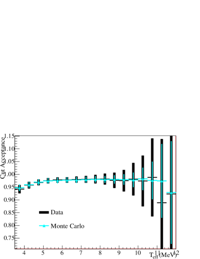
XI Trigger Efficiency

As discussed in Sec. IV, the primary trigger for SNO was a coincidence of PMT hits within a 93 ns time window, set to $N_{\rm coinc}=18$ hits for the early part of Phase I and to $N_{\rm coinc}=16$ hits for the remainder of Phase I and all of Phase II. We define the ‘efficiency’ of the trigger as the probability that an event with $N_{\rm coinc}$ hits actually triggered the detector. Small shifts in the analog (DC-coupled) baseline, noise, and disabled trigger electronics channels could all lead to a non-unity efficiency. We measured the efficiency using the isotropic laser source, by triggering on the laser pulse and comparing an offline evaluation of the trigger (by counting hits in a sliding 93 ns window) to the output of the hardware trigger. We found that for the $N_{\rm coinc}=18$ hit threshold, events with 23 or more hits in coincidence triggered the detector with an efficiency greater than 99.9% and, for the $N_{\rm coinc}=16$ hit threshold, the efficiency reached 99.9% at 21 hits. Figure 19 shows the efficiency measured as a function of $N_{\rm coinc}$, for Phase I at the higher $N_{\rm coinc}=18$ threshold, and for Phase II at the lower $N_{\rm coinc}=16$ hit threshold.

Figure 19: Comparison of the trigger efficiencies in the two data-taking phases and for the two different thresholds used.

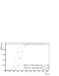
For events at our $T=3.5$ MeV analysis threshold, the mean number of hits in an event over the full 400 ns event window was $\sim$ 30 for Phase I and $\sim$ 27 for Phase II, with RMS’s of 1.8 hits and 1.7 hits, respectively. The numbers of hits in the 400 ns event window and in the 93 ns trigger coincidence window differed primarily in the contribution from random PMT noise which, for both phases, contributed on average roughly 1 additional hit in the 400 ns event window. Thus, for both phases, the trigger efficiency was above 99.9% for all but a negligible fraction of events with a high enough $N_{\rm coinc}$ to pass the analysis cuts.

Because our PDFs and overall normalization were derived from simulation, we compared the trigger-efficiency estimate from the data to the simulation’s prediction. We also compared the idealized simulated trigger to a simulation that included variations in the trigger baseline as measured by an online monitor. We found that the Monte Carlo simulation’s prediction of trigger efficiency was in excellent agreement with our measurement for both SNO phases, and that the measured variations contributed a negligible additional uncertainty to our overall acceptance.

XII Uncertainties on the Neutron Capture Efficiencies

In Phase I, neutrons produced through the NC reaction and background processes were captured on deuterons within the heavy water, releasing a single 6.25 MeV $\gamma$ ray. In Phase II, the neutrons were captured primarily on ³⁵Cl, releasing a $\gamma$ cascade of total energy 8.6 MeV. The absolute cross sections for these capture reactions, along with detector acceptance, determined the rate of detected neutron events. The uncertainty on the neutron capture efficiency for Phase II overwhelmingly dominates that for Phase I in the final flux determinations because of the larger capture cross section.

In this analysis, we used the Monte Carlo simulation to define the central values of the neutron capture efficiencies. Included in our simulation were the measured isotopic purity of the heavy water, as well as its density and temperature and, for Phase II, the measured density of salt added to the D₂O.

To assess the systematic uncertainties on the neutron capture efficiencies, we used data taken with the ²⁵²Cf source deployed at many positions throughout the detector, and compared the observed counting rates to simulations of the source runs. The differences between data and simulated events provide an estimate of the simulation’s accuracy. The Phase I and Phase II data sets are noticeably different in their neutron detection efficiency because of the much larger capture cross section in Phase II, and the higher energy $\gamma$ cascade from neutron capture on chlorine. We therefore assessed the uncertainties in the two phases slightly differently, as discussed below. We also compared the results of this ‘direct counting’ approach with a ‘time series analysis’, in which the relative times of events were used to extract the capture efficiency. The two methods were in excellent agreement for both phases. Our capture efficiency uncertainty for Phase II is $\pm 1.4$%, and for Phase I it is $\pm$2%.

XII.1 Phase II Neutron Capture Efficiency Uncertainties

For the Phase II analysis, neutron events from the ²⁵²Cf source were selected using the same burst algorithm that was used in previous SNO publications nsp . Neutrons were identified by looking for prompt fission $\gamma$ events from the ²⁵²Cf decay, and tagging subsequent events that occurred within 40 ms. Figure 20 plots the neutron detection efficiency for each source run as a function of radial position of the source in the detector, for both data and Monte Carlo simulated events. The source position for a run was determined by finding the mean reconstructed position of the prompt fission $\gamma$ events, to eliminate the large positioning uncertainties of the source deployment mechanism. The efficiencies shown in Fig. 20 were each fitted to a phenomenologically-motivated neutron detection efficiency function:

$$\epsilon(s)=A({\rm tanh}(B(s-C))-1),$$ (12)

where $\epsilon(s)$ gives the neutron capture efficiency at source radius $s$.

Figure 20: (Color online) Data and Monte Carlo neutron detection efficiencies in Phase II fitted to the phenomenologically-motivated neutron detection efficiency function.

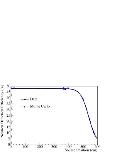
To determine the uncertainty on the simulation’s prediction of capture efficiency, we first calculated the mean capture efficiency in the D₂O volume, given the two functions shown in Fig. 20, as follows:

$$\epsilon=\frac{\int_{0}^{600.5}s^{2}\epsilon(s)ds}{\int_{0}^{600.5}s^{2}ds}.$$ (13)

We took the difference of 0.8% between data and simulation as a baseline uncertainty. (The mean detection efficiency measured this way was 35.6%).

The normalization of the curves shown in Fig. 20 depends on the strength of the ²⁵²Cf source, which we know to 0.7% based on ex-situ measurements. An overall shift in reconstructed event positions, discussed in Sec. VI, also changed the measured efficiency in data relative to the simulation results. By varying the value of this shift within its range of uncertainty we found it resulted in an additional 0.3% uncertainty in capture efficiency. The uncertainty in the fit parameters of the neutron detection efficiency function was included conservatively by taking the entire statistical uncertainty on the data efficiency measurements of Fig. 20, which yields another 0.9%. Lastly, we included a 0.1% uncertainty to account for the fraction of ²⁵⁰Cf in the ²⁵²Cf source (only ²⁵²Cf is simulated by the Monte Carlo code). The overall uncertainty on the neutron capture efficiency, calculated by adding these in quadrature, was 1.4%.

We checked these results by performing an independent time series analysis, in which we fit directly for the efficiency at each source deployment point based on the rates of neutron capture and $\gamma$ fission events (the source strength is not an input parameter). The fit included parameters associated with the overall fission rate, backgrounds from accidental coincidences, and the mean capture time for neutrons. We obtained the efficiency as a function of source radial position, to which we fit the same efficiency function from Eq. 12, and extracted the volume-weighted capture efficiency directly (rather than by comparison to Monte Carlo). The mean efficiency calculated this way was $35.3\pm 0.6$%, in excellent agreement with the value of 35.6% from the direct counting method, and well within the uncertainties on both measurements.

XII.2 Phase I Neutron Capture Efficiency Uncertainties

The measurement of neutron capture efficiency uncertainty for Phase I is more difficult than for Phase II, primarily because the lower capture cross section in Phase I made identification of neutron events from the ²⁵²Cf source difficult. The number of detected neutrons per fission was small (less than one on average), and the long capture time (roughly 50 ms) made coincidences more likely to be accidental pile-up of prompt fission $\gamma$s than neutrons following the $\gamma$s.

Instead of using the burst algorithm, we separated neutron events from fission $\gamma$s based on their differing energies and mean free paths in D₂O. Events were required to be more than 150 cm from the source position and to have energies above the mean energy expected for a neutron capture event, for both data and Monte Carlo events. The detected rate of events after these cuts was used for the data and Monte Carlo simulation comparison.

An additional parameter was added to the neutron detection efficiency function for these data, as follows:

$$\epsilon(s)=A({\rm tanh}(B(s-C))-D),$$ (14)

and the resulting fits to data and Monte Carlo are shown in Figure 21.

Figure 21: (Color online) Comparison of the fit functions to the data and Monte Carlo in Phase I.

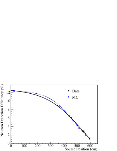
The difference of the volume-weighted integrals of the two curves is just 0.9%, but the small value is clearly due to cancellation differences at different radii. The shape difference is driven by small differences between the data and Monte Carlo fits at large radii, which are likely due to unassessed systematic errors on the data points themselves. We included additional uncertainties to account for these. In particular, we included a 0.6% uncertainty associated with the statistical uncertainties of the data and Monte Carlo neutron detection efficiency function parameters, and an additional 0.6% uncertainty associated with knowledge of the source position. We also included a further uncertainty of 0.9% to account for data and Monte Carlo differences in the energy cut applied to select neutrons.

We applied the same source-strength uncertainties as for the Phase II analysis, namely the 0.7% absolute source strength calibration, and 0.1% from the (unmodeled) contamination of ²⁵⁰Cf in the ²⁵²Cf source. The total uncertainty on the neutron capture efficiency for Phase I comes to 2%.

To check our estimates, we also performed a time series analysis of the ²⁵²Cf data. Unlike Phase II, for Phase I we cannot extract the absolute efficiency to compare with that derived from the direct counting method because of the 150 cm reconstruction cut. Instead, we performed the time series analysis on both Monte Carlo and source data runs, and compared them. We found the fractional difference between the source-derived and Monte Carlo-derived efficiencies to be just 0.3%, well within the 2% uncertainty obtained from the direct counting method. One output of the time series analysis is the neutron capture time: the time between neutron emission from the ²⁵²Cf source and capture on a deuteron. Figure 22 shows the neutron capture time as a function of source radial position for both data and Monte Carlo. As the ²⁵²Cf source approaches the acrylic vessel and light water region, the capture time decreases significantly. The overall agreement between the measured capture times in data and Monte Carlo is very good throughout most of the volume.

Figure 22: (Color online) Mean neutron capture time from the time series analysis in Phase I as a function of source position. The line shows the best fit to the simulation using a cubic polynomial.

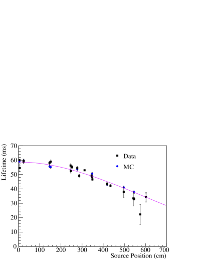
XIII Backgrounds

Lowering the energy threshold opened the analysis window to additional background contamination, predominantly from radioactive decays of ²¹⁴Bi and ²⁰⁸Tl in the ²³⁸U and ²³²Th chains, respectively. In Phase II, neutron capture on ²³Na produced a low level of ²⁴Na in the detector which, in its decay to ²⁴Mg, produced a low energy $\beta$ and two $\gamma$s. One of these $\gamma$s has an energy of 2.75 MeV, which could photodisintegrate a deuteron. The result was some additional electron-like and neutron capture background events. In addition, radon progeny that accumulated on the surface of the AV during construction could have created neutrons through ($\alpha$,$n$) reactions on isotopes of carbon and oxygen within the acrylic.

In the past, most of these backgrounds were estimated using separate self-contained analyses and then subtracted from the measured neutrino fluxes. In this analysis, the Monte Carlo simulation was used to create PDFs for each of 17 sources of background events (except for PMT $\beta$-$\gamma$ events, for which an analytic PDF was used in each phase, as described in Sec. XIII.3), and the numbers of events of each type were parameters in the signal extraction fits. Table 10 lists the sources of physics-related backgrounds that were included in the fits.

Detector Region	Phase I	Phase II
D2O volume	Internal 214Bi	Internal 214Bi
	Internal 208Tl	Internal 208Tl
		24Na
Acrylic vessel	Bulk 214Bi	Bulk 214Bi
	Bulk 208Tl	Bulk 208Tl
	Surface ($\alpha$,$n$) $n$s	Surface ($\alpha$,$n$) $n$s
H2O volume	External 214Bi	External 214Bi
	External 208Tl	External 208Tl
	PMT $\beta$-$\gamma$s	PMT $\beta$-$\gamma$s

Table 10: The sources of physics-related background events in the LETA analysis.

All of the Monte Carlo-generated PDFs were verified using calibration sources. Ex-situ measurements htio ; mnox of background levels in the D₂O and H₂O provided a priori information for several of them, which were used as constraints in the signal extraction fits. In addition, corrections were applied after the signal extraction fits to account for a number of background event types that contributed much smaller levels of contamination. The following sections describe these procedures.

XIII.1 Background PDFs

Most of the PDFs used in the signal extraction were created from Monte Carlo simulations of the specific event types. However, because of the limited number of simulated PMT $\beta$-$\gamma$ events available in the radial range of interest, an analytic parameterization of the PDF was used, as described in Sec. XIII.3. This was verified by comparison to the simulation and uncertainties associated with the value of each parameter were propagated in the signal extraction fits.

The remainder of the background PDFs were verified by comparison of calibration data to simulated events. The D₂O and H₂O backgrounds were verified using the D₂O- and H₂O-region radon spikes in Phase II and calibration sources deployed in these regions. Bulk AV backgrounds were verified using the ²³⁸U and ²³²Th sources, and surface ($\alpha$,$n$) neutrons using the ²⁵²Cf source deployed near the AV.

In all cases, the data and Monte Carlo event distributions agreed to within the systematic uncertainties already defined for the PDFs. Figure 23 shows the energy dimension of a fit to the internal radon spike. The fit was performed using the unbinned signal extraction code (see Sec. XIV.3) in a simplified configuration, as described in Sec. VIII.3.1. The result is a good fit to the data, in particular at low energy. Figure 24 shows a comparison of data to simulation for the ²³²Th source deployed near the AV. A band is shown for the simulated events, representing the quadrature sum of the statistical uncertainties with the effect of applying the dominant systematic uncertainties. The distributions in $T_{\rm eff}$, $R^{3}$ and $\beta_{14}$ show good agreement within the 1$\sigma$ uncertainties.

Figure 23: (Color online) One dimensional projection of the fit to the internal radon spike data.

Figure 24: (Color online) Comparison of data to simulation for ²³²Th source runs near the AV in Phase II, in (a) $T_{\rm eff}$, (b) $R^{3}$, and (c) $\beta_{14}$. The band represents the 1$\sigma$ uncertainty on the Monte Carlo-prediction, taking the quadrature sum of the statistical uncertainties with the effect of applying the dominant systematic uncertainties.

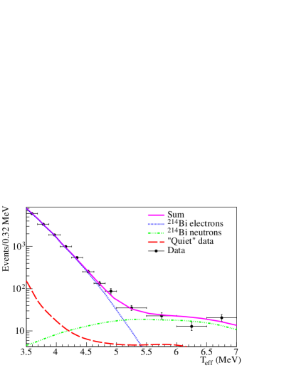
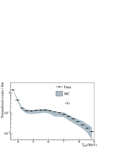
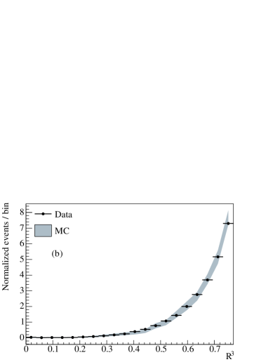
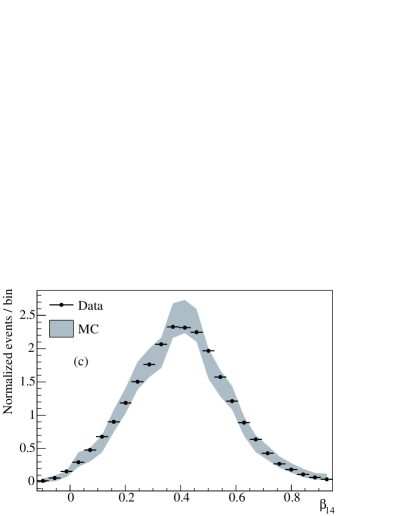
The cross section for photodisintegration affects the relative normalization of the neutron and electron parts of the background PDFs. The simulation used a theoretical value for the cross section and the associated 2% uncertainty was propagated in the signal extraction fits.

The simulation of ²⁴Na events used to generate a PDF was done under the assumption of a uniform distribution of events within the detector, since a primary source of ²⁴Na was the capture of neutrons produced by deployed calibration sources on ²³Na. ²⁴Na was also introduced via the neck, and via the water systems, which connected near the top and bottom of the AV. Therefore, the signal extraction fits were redone with different spatial distributions, in which the events originated either at the neck of the AV or at the bottom, with a conservatively chosen 10% linear gradient along the $z$-axis. The difference from the baseline (uniform distribution) fit was taken as a systematic uncertainty.

XIII.2 Low Energy Background Constraints

Several radioassays were performed during data taking to measure the concentrations of radon and radium in the D₂O and H₂O regions, as described in previous publications longd2o ; htio ; mnox . Although equilibrium was broken in the decay chains, the results are expressed in terms of equivalent amounts of ²³⁸U and ²³²Th assuming equilibrium for ease of comparison with other measurements. The results were used to place constraints on the expected number of background events in the analysis window. During Phase II, there was a leak in the assay system used to measure the ²³⁸U chain contamination that was not discovered until after data taking had ended, so there is no accurate constraint on the ²³⁸U level in the D₂O during that phase. Other limits based on secondary assay techniques were found to be too loose to have any impact on the signal extraction results and so were disregarded. The results of the assays are given in tables 11 and 12.

Phase	Isotope	Concentration ($\times$ 10-15 g/g of D2O)
I	238U	10.1$\,{}^{+3.4}_{-2.0}$
	232Th	2.09$\,\pm\,$0.21(stat)$\,{}^{+0.96}_{-0.91}$(syst)
II	238U	—
	232Th	1.76$\,\pm\,$0.44(stat)$\,{}^{+0.70}_{-0.94}$(syst)

Table 11: ²³⁸U and ²³²Th concentrations in the D₂O volume, determined from ex-situ radioassays in Phases I and II.

Phase	Isotope	Concentration (g/g of H2O)
I	238U	29.5$\,\pm\,$ 5.1$\times$ 10-14
	232Th	8.1$\,{}^{+2.7}_{-2.3}$$\times$ 10-14
II	238U	20.6$\,\pm\,$ 5.0$\times$ 10-14
	232Th	5.2$\,\pm\,$ 1.6$\times$ 10-14

Table 12: ²³⁸U and ²³²Th concentrations in the H₂O volume, determined from ex-situ radioassays in Phases I and II.

These concentrations were converted into an expected number of events and were applied as constraints in the signal extraction fits, as described in Sec. XIV.5.

In-situ analyses simsthesis were used to predict the number of background events from ²⁴Na decays in Phase II. The predicted value of $392\pm 117.6$ events was applied as a constraint in the signal extraction fits.

XIII.3 PMT $\beta$-$\gamma$ PDF

We use the term “PMT events” to refer to all radioactive decays in the spherical shell region encompassing the PMTs and the PSUP. These events were primarily ²⁰⁸Tl decays originating from ²³²Th contamination in the PMT/PSUP components.

PMT events occurred at a high rate, but only a tiny fraction of them reconstructed inside the signal box and within the fiducial volume: in Phase I, the acceptance was only $1.7\times 10^{-8}$ and in Phase II it was $5.9\times 10^{-8}$. Therefore, an enormous amount of computer time would be needed to generate enough events to create a PDF. Creation of a multi-dimensional PDF based entirely on simulation was therefore deemed to be impractical.

A high rate thorium source was deployed near the PSUP in both phases to help model these events. However, interpretation of this data was complicated by the fact that a point source with a sufficiently high rate tends to produce significant ‘pile-up’ of multiple events that trigger in the same time window. This pile-up changes the topology of the events to the extent that they are not characteristic of PMT $\beta$-$\gamma$s, so they cannot be used directly as a model.

Therefore, an analytic parameterization of the PDF, given in Eq. (15), was used. For this, the $\cos\theta_{\odot}$ dimension was assumed to be flat; the remaining three-dimensional PDF was of the form:

$$P_{PMT}(T_{\rm eff}, \beta_{14} ,R^{3})=e^{A\,T_{\rm eff}}\times(e^{B\,R^{3}}+C)$$ (15)

$$\times \mathcal{N}(\beta_{14}\,|\,\bar{\beta}_{14}=D+ER^{3},\sigma=F),$$

where $\mathcal{N}(x|\bar{x},\sigma)$ is a Gaussian distribution in $x$ with mean $\bar{x}$ and standard deviation $\sigma$. The $\beta_{14}$ dimension was determined from a Gaussian fit to Monte Carlo events, in which $\bar{\beta}_{14}$ was allowed a linear dependence on $R^{3}$.

The source location of the PMT events, their large number, and the fact that they must reconstruct nearly 3 m from their origin to appear inside the fiducial volume means that they have features that distinguish them from other sources of backgrounds. Therefore, we were able to extract a prediction for the total number of PMT events, as well as for the shape of the energy and radial dimensions of the PDF, from the data itself, by performing a bifurcated analysis.

In a bifurcated analysis, two independent cuts are selected that discriminate signal from background. The behavior of these cuts when applied both separately and in combination is used to assess the number of signal and background events in the analysis window. We assume that the data set consists of $\nu$ signal events and $\beta$ background events, so that the total number of events is $S=\beta+\nu$. The background contamination in the final signal sample is just the fraction of $\beta$ that passes both cuts. If the acceptances for background and signal events by cut $i$ are $y_{i}$ and $x_{i}$, respectively, the contamination is $y_{1}y_{2}\beta$ and the number of signal events is $x_{1}x_{2}\nu$.

Given the number, $a$, of events that pass both cuts, the number, $b$, that fail cut 1 but pass cut 2, and the number, $c$, that pass cut 1 but fail cut 2, we then relate these with a system of equations:

$$a+c = x_{1}\nu+y_{1}\beta,$$ (16)

$$a+b = x_{2}\nu+y_{2}\beta,$$ (17)

$$a = x_{1}x_{2}\nu+y_{1}y_{2}\beta,$$ (18)

$$\beta+\nu = S,$$ (19)

which we solve analytically, using Monte Carlo-predictions for the cut acceptances, to determine the contamination, $K=y_{1}y_{2}\beta$, in the signal sample. A feature of this method is that it produces a contamination estimate without including events from the signal box (those that pass both cuts) in the analysis.

In this analysis, the ‘background’ comprised the PMT events and the ‘signal’ all other events, including both neutrino interactions and non-PMT radioactive decays. The cuts chosen were the in-time ratio (ITR) cut, because it selected events that were reconstructed far from their true origin, and the early charge (EQ) cut because it selected events in which a large amount of light produced hits early in time in a small number of tubes. These tend to be characteristics of PMT events (see Sec. X.2).

For a bifurcated analysis to work, the probabilities of passing the cuts must be statistically independent. To demonstrate this, we loosened the cuts, and found that the increase in the number of background events agreed well with what would be expected if they were independent.

One result of the bifurcated analysis is a prediction for the number of PMT events in the analysis window, which was used as a constraint in the binned likelihood signal extraction fits, as described in Sec. XIV.5.

The acceptance of signal events ($x_{1}x_{2}$) $\neq 1.0$ and therefore some non-PMT events were also removed by the cuts. Such events falsely increase the count of background events in the three ‘background boxes’. We limited the impact of this effect by restricting the analysis to the 3.5–4.5 MeV region, which was overwhelmingly dominated by PMT events. We also included a correction for the number of non-PMT events in each of the background boxes by using estimates from the Monte Carlo simulation for the acceptance of all other signals and backgrounds, and verifying these predictions with radon spike data. (²¹⁴Bi, a radon daughter, is the dominant background other than the PMT events in this region).

To estimate the number of non-PMT events in each of the three background boxes, we multiplied the Monte Carlo-predicted acceptances of non-PMT events by the expected total number of these events in the data set. The procedure was therefore iterative: a PMT PDF was created using initial estimates for the total number of non-PMT events in the data set and their acceptances; the bifurcated analysis was used to predict the number of PMT events in the signal box; the data were re-fit with this new PMT constraint; the total number of non-PMT events in the data set, based upon the new fit, was then used to update the non-PMT event correction in the background boxes in the bifurcated analysis, and so on. In practice, the bifurcated analysis itself was simply included within the signal extraction fit, so the prediction for the number of PMT events could be recalculated as the fit progressed, and the penalty factor in the likelihood calculation from the resulting constraint could be varied accordingly. To determine systematic uncertainties on this overall procedure, we tested the analysis on sets of fake data and compared the prediction of the bifurcated analysis to the known true number of PMT $\beta$-$\gamma$ events in the signal box.

We verified the bifurcated analysis results by comparing the prediction of the total number of PMT $\beta$-$\gamma$ events in the signal box to an estimate made with an independent analysis performed outside the fiducial volume. This independent analysis looked for events that occurred at high radius and were inward-pointing, which are characteristics of PMT $\beta$-$\gamma$ events, and extrapolated that count into the fiducial volume. The measurements agreed with the bifurcated analysis to well within the uncertainties on the two methods.

To predict the shape of the PMT PDF, the bifurcated analysis was performed in discrete bins in $T_{\rm eff}$ and $R^{3}$. Unlike the prediction for the total number of PMT events in the data set, this calculation was not included in the signal extraction, so a fixed estimate of the contamination of non-PMT events in the three background boxes was applied. This estimate was derived from a signal extraction fit performed on a small subset of the data. To take uncertainties into account, bifurcated analyses were performed on Monte Carlo-generated ‘fake’ data sets with the dominant systematic and statistical uncertainties applied in turn, to determine the effect of each on the extracted shape for the PMT PDF. The differences of the results from the unshifted version were added in quadrature to obtain an additional uncertainty on the shape.

A number of functional forms were fit to the $T_{\rm eff}$ and $R^{3}$ distributions to determine the best parameterizations for the shapes. An exponential was found to be a good fit to the energy profile and an exponential plus a constant offset to the radial distribution (see Eq. (15)). The fit results for Phase II are shown in Figure 25.

Figure 25: (Color online) Predicted shapes for the PMT PDF in (a) $R^{3}$ and (b) $T_{\rm eff}$ in Phase II.

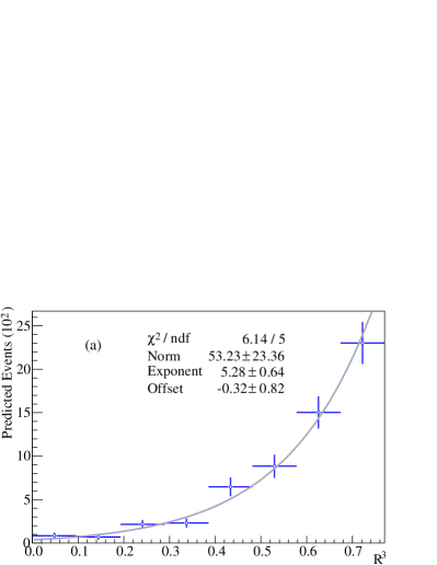
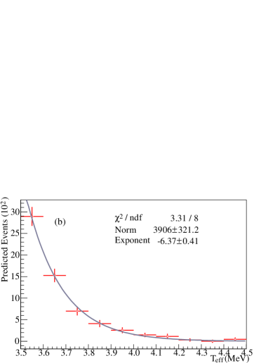
The parameters from the fits shown in Fig. 25 were varied in the signal extraction by applying a Gaussian penalty factor to the likelihood function, as described in Sec. XIV.5. The mean of the Gaussian was the central fit value from Fig. 25 and the standard deviation was taken as the total uncertainty in this value, including both the fit uncertainty from Fig. 25 and the additional systematic uncertainties described above. Results for both phases are shown in Table 13. The fits to the bifurcated analysis prediction for the $R^{3}$ distribution showed a significant correlation between the exponent and the offset, with correlation coefficients of 0.846 and 0.883 in Phases I and II, respectively. This correlation was included in the Gaussian penalty factor in the signal extraction fits.

Parameter	Phase I	Phase II
Energy exponent, A (/MeV)	$-$5.94 $\pm$ 0.96	$-$6.37 $\pm$ 0.81
$R^{3}$ exponent, B	5.83 $\pm$ 0.96	5.28 $\pm$ 0.79
$R^{3}$ offset, C	$-$0.40 $\pm$ 1.43	$-$0.32 $\pm$ 1.16

Table 13: Parameters defining the PMT PDF shape, as defined in Eq. (15).

XIII.4 Limits on Instrumental Backgrounds

Because instrumental background events were not modeled by the simulation, their contamination in the analysis window was determined directly from the data. A bifurcated analysis was used, similar to that described in Sec. XIII.3. In this instance, two sets of cuts were used to define the analysis: the instrumental cuts and the high-level cuts, described in Sec. X. The numbers of events in the data set failing each and both sets of cuts were used to estimate the contamination by instrumental backgrounds.

As was done in Sec. XIII.3, a prediction of the number of good (physics) events that failed the instrumental cuts was used to correct the number of events in each of the background boxes. We obtained this prediction using the cut acceptances given in Sec. X.5.1 and an estimate of the numbers of signal and radioactive background events in the data set. The analysis was performed at two energy thresholds in order to study the energy dependence of the contamination. Results are given in Table 14.

	Threshold
Phase	3.5 MeV	4.0 MeV
I	2.64 $\pm$ 0.22	0.09 $\pm$ 0.42
II	4.48 $\pm$ 0.27	0.52 $\pm$ 0.23

Table 14: Estimated number of instrumental contamination events in the full data set at different analysis thresholds.

Since these events were not modeled in the simulation, it is difficult to directly predict their effect on the signal extraction fit results. However, because virtually all of them fall into the lowest energy bin, they are unlikely to appear like neutron events. Since the $T_{\rm eff}$ distributions of CC and ES signals were unconstrained in the signal extraction fit, they could mimic these event types. Therefore, a conservative approach was taken, in which the estimated contamination from the 3.5 MeV analysis was applied as an additional uncertainty in the lowest energy bin for both the CC and ES signals.

XIII.5 Atmospheric Backgrounds

The NUANCE neutrino Monte Carlo simulation package nuance was used to determine the contribution of atmospheric neutrino events to the data set. The estimated number of atmospheric neutrino events was not large enough to merit introducing an additional event type into the already complex signal extraction procedure. Instead, 15 artificial data sets were created that closely represented the best estimate for the real data set, including all neutrino signals and radioactive backgrounds in their expected proportions. The NUANCE simulation was used to predict the distribution of atmospheric neutrino events in each of the four observable parameters used to distinguish events in the signal extraction fit (see Sec. XIV), and a number of such events were included in each artificial data set, drawn from the estimate for the number in the true data. Signal extraction was performed on these sets to determine which signal the events would mimic in the extraction. This resulted in a small correction to the NC flux of $4.66\pm 0.76$ and $17.27\pm 2.83$ events to be subtracted in Phases I and II, respectively, and small additional uncertainties for the CC and ES rates, mostly at the sub-percent level.

Atmospheric events were often characterized by a high-energy primary followed by several neutrons. Therefore, there was significant overlap with events identified by the ‘coincidence cut’, which removed events that occurred within a fixed time period of each other. This overlap was exploited to verify the predicted number of atmospheric events. Without application of the coincidence cut, a total of $28.2\pm 5.4$ and $83.9\pm 15.9$ atmospheric neutrino events were predicted in Phases I and II, respectively. The coincidence cut reduced these numbers to $21.3\pm 4.0$ and $29.8\pm 5.7$ events, which were the numbers used in the creation of the initial artificial data sets. A second group of sets was created, using the pre-coincidence cut estimates for the number of events, to determine the change in the NC flux due to the additional events. The signal extraction was then performed on a subset of the real data, both with and without the application of the coincidence cut, and the observed difference in the NC flux was entirely consistent with the predictions, thus verifying the method used to derive the NC flux correction.

XIII.6 Isotropic Acrylic Vessel Background (IAVB)

Early in the SNO analyses, a type of instrumental background was discovered that reconstructed near the AV and was characterized by very isotropic events ($\beta_{14}<0.15$). At higher energies ($N_{\rm hit}>60$), these events form a distinct peak in a histogram of $\beta_{14}$, and they are easily removed from the data by a combination of the fiducial volume and isotropy cuts. However, at lower energies, position reconstruction errors increase and the isotropy distributions of the IAVB and other events broaden and join, so that removal of the IAVB events by these cuts is no longer assured.

Accurate simulation of these events is difficult because the physical mechanism that produces the IAVB events has not been identified and crucial IAVB event characteristics cannot be predicted. These include the light spectrum, photon timing distribution, location, and effective event energy. To circumvent this problem, simulated events were generated that covered a wide range of possibilities. Three event locations were modeled: on the exterior and interior AV surfaces, and uniformly distributed within the AV acrylic. Events were generated at three different photon wavelengths that cover the range of SNO detector sensitivity: 335, 400, and 500 nm. The photons were generated isotropically, with the number of photons in an event chosen from a uniform distribution with a maximum above the energy range used in the neutrino analysis. The photon time distribution was a negative exponential, with the time constant for an event chosen from a truncated Gaussian with mean and standard deviation of 5 ns.

Using PDFs derived from the simulated event samples, maximum likelihood signal extraction code was used to estimate the number of IAVB events in the data in the vicinity of the AV, between 570 and 630 cm from the detector center, in accompaniment with the CC, ES, and NC neutrino event types and ²⁰⁸Tl and ²¹⁴Bi backgrounds in the D₂O, AV, H₂O, and PMTs. This was done separately for each of the nine simulated photon wavelength/event location combinations. Because the energy distribution of the IAVB events was unknown, the IAVB extractions were done as a function of N_hit in 11 bins. The ratio of the number of IAVB events that passed all the neutrino cuts to those that fit near the AV in each N_hit bin was calculated for each simulated IAVB case as a function of event energy. These ratios were used, together with the estimated numbers of such events near the AV, to estimate the IAVB contamination in the neutrino sample as a function of energy for each of the simulated IAVB cases.

The polar-angle distributions of hit PMTs in the simulated IAVB events were studied in a coordinate system centered on the middle of the AV, with its $z$-axis along the radial vector through the fitted event location. There are marked differences in these distributions among the different simulated cases due to optical effects of the AV. Comparisons of these distributions were made between simulated events and high N_hit, high isotropy events in the data that reconstruct near the AV (presumed to be IAVB events). A fit was made to find the weighted combination of the simulated cases that best fit the high N_hit data. The resulting weights were assumed to be valid at all energies, and were used together with the contamination ratios discussed above: first, to estimate the total IAVB background expected in the neutrino analysis data set as a function of energy (totaling 27 and 32 events above 3.5 MeV in Phases I and II, respectively) and, second, to generate a set of simulated IAVB events representative of those expected to contaminate the neutrino data.

A test similar to that described in Sec. XIII.5 was performed. Fifteen artificial data sets were created that also contained simulated IAVB events based on estimates of the weighted contributions of the simulated cases and their energy distributions. It was found that the majority of the IAVB events fit out as other background event types, so that the result of adding the simulated IAVB background was only small additional uncertainties for each of the neutrino flux parameters, with no required corrections. The increase in uncertainty for the NC flux was evaluated at $0.26\%$. The increases of the CC uncertainties were also mostly at the sub-percent level, and the increase in uncertainties on the ES rates were so small as to be negligible ($<0.01\%$).

XIII.7 Additional Neutron Backgrounds

A full study of other possible sources of neutron background events, such as from events such as ($\alpha$,$n$) reactions and terrestrial and reactor antineutrino interactions, was presented in previous publications longd2o ; nsp . The full set of simulated NC events was used to adjust these numbers for the lowered energy threshold and for the live times and detection efficiencies in the two phases to give a final correction to the NC flux of $3.2\pm 0.8$ and $12.0\pm 3.1$ neutron capture events in Phases I and II, respectively.

XIV Signal Extraction Methods

An extended maximum likelihood method was used to separate event types based on four observable parameters: the effective electron kinetic energy, $T_{\rm eff}$; the angle of the event direction with respect to the vector from the Sun, $\cos\theta_{\odot}$; the normalized cube of the radial position in the detector, $R^{3}$; and the isotropy of the PMT hits, $\beta_{14}$. Two independent techniques were used, as described in sections XIV.2 and XIV.3. One method used binned PDFs and the other an unbinned, “kernel estimation” approach.

We performed two distinct types of fit. The first extracted the detected electron energy spectra for CC and ES events in individual $T_{\rm eff}$ bins, without any model constraints on the shape of the underlying neutrino spectrum. We refer to this as an ‘unconstrained’ fit. The second fit exploited the unique capabilities of the SNO detector to directly extract the energy-dependent $\nu_{e}$ survival probability (Sec. XIV.4). The survival probability was parameterized as a polynomial function and applied as a distortion to the ⁸B neutrino energy spectrum (taken from winter ). The shapes of the CC and ES $T_{\rm eff}$ spectra were recomputed from the distorted ⁸B spectrum as the fit progressed, allowing the polynomial parameters to vary in the fit. The overall fluxes were also constrained in this fit through the requirement of unitarity. The features in common for the two signal extraction approaches are described below.

The types of events included in the fit were the three neutrino interaction types (CC, ES and NC) and 17 background event types across the two phases of data, as defined in Table 10. The likelihood was maximized with respect to the number of events of each signal type, and several systematic parameters affecting the shapes of the PDFs, as described in Sections XIV.2 and XIV.3.

To extract energy spectra for the CC and ES neutrino signals in the unconstrained fits, CC and ES PDFs were created in discrete $T_{\rm eff}$ intervals and the fitted numbers of events in these intervals were allowed to vary independently. The energy spectra for events from the NC interaction and from radioactive backgrounds have no dependence on the neutrino oscillation model, and so the shapes of these spectra were fixed within their systematic uncertainties.

The flux of solar neutrinos was assumed to be constant, so a single set of neutrino-related fit parameters was applied to both phases. Therefore, the neutrino signal parameters varied in the fit were an NC rate and a number of CC and ES rates in discrete energy intervals, as defined in Sections XIV.2 and XIV.3. Although SNO was primarily sensitive to the ⁸B chain of solar neutrinos, we included a fixed contribution of solar hep neutrinos, which was not varied in the fit. Based on results from a previous SNO analysis nsp , we used 0.35, 0.47, and 1.0 times the Solar Standard Model (SSM) prediction for CC, ES, and NC hep neutrinos, respectively. Taken together, these correspond to 16.4 events in Phase I and 33.3 events in Phase II.

To take into account correlations between parameters, multi-dimensional PDFs were used for all signals. In the unconstrained fits, CC and ES were already divided into discrete energy bins, and three-dimensional PDFs were created in each bin for the other observables: $P(\beta_{14},R^{3},\cos\theta_{\odot})$. In the survival probability fits, fully four-dimensional PDFs were used for CC and ES events. For the NC and background PDFs the $\cos\theta_{\odot}$ distribution is expected to be flat, since there should be no dependence of event direction on the Sun’s position, but correlations exist between the other observables. For these event types, the PDFs were factorized as $P(T_{\rm eff},\beta_{14},R^{3})\times P(\cos\theta_{\odot})$.

Uncertainties in the distributions of the observables were treated as parameterized distortions of the Monte Carlo PDF shapes. The dominant systematic uncertainties were allowed to vary in the fit in both signal extraction methods. Less significant systematics were treated as in previous SNO analyses longd2o , using a ‘shift-and-refit’ approach: the data were refit twice for each systematic uncertainty, with the model PDFs perturbed by the estimated positive and negative 1 $\sigma$ values for the uncertainty in a given parameter. The differences between the nominal flux values and those obtained with the shifted PDFs were taken to represent the 68% C.L. uncertainties, and the individual systematic uncertainties were then combined in quadrature to obtain total uncertainties for the fluxes.

XIV.1 Systematic Uncertainties: Phase Correlations

Uncertainties related to theoretical quantities that are unaffected by detector conditions (such as the photodisintegration cross section uncertainty) were applied to both phases equally. Uncertainties in quantities dependent on detector conditions (such as energy resolution) were treated independently in each phase. Uncertainties in quantities that partly depend on the operational phase (such as neutron capture efficiency, which depends both on a common knowledge of the ²⁵²Cf source strength and on the current detector conditions) were treated as partially correlated. For the latter, the overall uncertainty associated with each phase thus involved a common contribution in addition to a phase-specific uncertainty. Since neutron capture events were more similar to electron-like events in Phase I than in Phase II, several of the neutron-related uncertainties applied to Phase II only. The correlations are summarized in Table 15.

Systematic uncertainty	Correlation
Energy scale	Both
Electron energy resolution	Uncorrelated
Neutron energy resolution	Phase II only
Energy linearity	Correlated
$\beta_{14}$ electron scale	Correlated
$\beta_{14}$ neutron scale	Phase II only
$\beta_{14}$ electron width	Correlated
$\beta_{14}$ neutron width	Phase II only
$\beta_{14}$ energy dependence	Correlated
Axial scaling	Uncorrelated
$z$ scaling	Uncorrelated
$x$, $y$, $z$ offsets	Uncorrelated
$x$, $y$, $z$ resolutions	Uncorrelated
Energy dependent fiducial volume	Uncorrelated
$\cos\theta_{\odot}$ resolution	Uncorrelated
PMT $T_{\rm eff}$ exponent	Uncorrelated
PMT $R^{3}$ exponent	Uncorrelated
PMT $R^{3}$ offset	Uncorrelated
PMT $\beta_{14}$ intercept	Uncorrelated
PMT $\beta_{14}$ radial slope	Uncorrelated
PMT $\beta_{14}$ width	Uncorrelated
Neutron capture	Both
Photodisintegration	Correlated
24Na distribution	Phase II only
Sacrifice	Uncorrelated
IAVB	Uncorrelated
Atmospherics backgrounds	Uncorrelated
Instrumental contamination	Uncorrelated
Other neutrons	Uncorrelated

Table 15: Phase correlations of the systematic uncertainties. “Correlated” refers to a correlation coefficient of 1.0 between the phases and “uncorrelated” refers to a coefficient of 0.0. “Both” means an uncertainty was treated as partially correlated between the phases.

XIV.2 Binned-Histogram Unconstrained Fit

In this approach, the PDFs were created as three-dimensional histograms binned in each observable dimension, as summarized in Table 16. For CC and ES, three-dimensional PDFs were created in each $T_{\rm eff}$ interval, to fully account for correlations between all four observable dimensions. Fifty rate parameters were fitted: the CC and ES rates in each of 16 spectral bins, the NC normalization and 17 background PDF normalizations. Dominant systematic uncertainties were allowed to vary within their uncertainties, or ‘floated’, by performing one-dimensional scans of the likelihood in the value of each systematic parameter. This involved performing the fit multiple times at defined intervals in each systematic parameter and extracting the value of the likelihood, which included a Gaussian factor whose width was defined by the independently estimated uncertainty on that parameter, as described in Sec. XIV.5. This combined a priori knowledge from the calibration data and Monte Carlo studies used to parameterize systematic uncertainties with information inherent in the data itself. If a new likelihood maximum was found at an offset from the existing best estimate of a particular systematic parameter, then the offset point was defined as the new best estimate. An iterative procedure was used to take into account possible correlations between parameters. The final uncertainties on each parameter were defined by where the log likelihood was 0.5 less than at the best-fit point, and the differences in each fitted flux parameter between these points and the best-fit point were taken as the associated systematic uncertainties for that parameter. For more details of this approach, see orebithesis .

Observable		Min	Max	Bins	Bin width
CC, ES $T_{\rm eff}$		3.5 MeV	11.5 MeV	16	0.5 MeV
Other $T_{\rm eff}$		3.5 MeV	5.0 MeV	6	0.25 MeV
		5.0 MeV	11.5 MeV	13	0.5 MeV
$\cos\theta_{\odot}$		$-$1.0	1.0	8	0.25
$R^{3}$		0.0	0.77025	5	0.15405
$\beta_{14}$		$-$0.12	0.95	15	0.0713

Table 16: PDF configurations used for the binned-histogram signal extraction approach.

The parameters floated using this approach, along with their relevant correlations, as described in Sec. XIV.1, were:

• Energy scale (both correlated and uncorrelated in each phase)

• Energy resolution (uncorrelated in each phase)

• $\beta_{14}$ scale for electron-like events (correlated between phases)

• PMT $\beta$-$\gamma$ $R^{3}$ exponent (uncorrelated in each phase, see Sec. XIII.3)

• PMT $\beta$-$\gamma$ $R^{3}$ offset (uncorrelated in each phase, see Sec. XIII.3)

• PMT $\beta$-$\gamma$ $T_{\rm eff}$ exponent (uncorrelated in each phase, see Sec. XIII.3)

The remaining systematic uncertainties were applied using the ‘shift-and-refit’ approach.

XIV.3 Unbinned Unconstrained Fit Using Kernel Estimation

In this approach, the PDFs were created by kernel estimation. Like standard histogramming techniques, kernel estimation starts with a sample of event values, $t_{i}$, drawn from an unknown distribution, $P(x)$. Based on this finite sample, the parent distribution is approximated by $\hat{P}(x)$, which is a sum of kernel functions, $K_{i}(x)$, each centered at an event value from the sample:

$$\hat{P}(x)=\frac{1}{n}\sum_{i=1}^{n}K_{i}(x-t_{i}).$$ (20)

The most common choice of form of kernel functions is the normalized Gaussian distribution,

$$K(x/h)=\frac{1}{h\sqrt{2\pi}}e^{-(x/h)^{2}/2},$$ (21)

where $h$ is called the bandwidth of the kernel. One can pick a different bandwidth, $h_{i}$, for the kernel centered over each event.

Kernel-estimated density functions have many useful properties. If the kernel functions are continuous, then the density function will also be continuous. In one dimension, kernel estimation can also be shown to converge to the true distribution slightly more quickly than a histogram with bin size the same as the kernel bandwidth. Generalizing the kernel estimation method to multiple dimensions is done by selecting a kernel with the same dimensionality as the PDF. We used a multi-dimensional Gaussian kernel that was simply the product of one-dimensional Gaussians. We followed the prescription given in cranmer for the selection of bandwidths for each event in each dimension.

By varying the values associated with the events in the PDF sample individually, kernel estimation can very naturally be extended to incorporate systematic variation of PDF shapes. For example, energy scale is incorporated by a transformation of the simulated event values, $t_{i}\rightarrow(1+\alpha)\times t_{i}$, where $\alpha$ is a continuously variable parameter. Such transformations preserve the continuity and analyticity of the PDF. We can then add these systematic distortion parameters to the likelihood function, and also optimize with respect to them using a gradient descent method. This allows correlations between systematics and neutrino signal parameters, as well as between systematics themselves, to be naturally handled by the optimization algorithm. In addition, the information in the neutrino data set itself helps to improve knowledge of detector systematics.

Three kinds of systematic distortions can be represented within this formalism. Transformations like energy scale and position offset have already been mentioned. A Gaussian resolution systematic can be floated by transforming the bandwidth, $h$, through analytic convolution. Finally, re-weighting systematics, such as the neutron capture efficiency, are represented by varying the weight of events in the sum.

The main challenge in using kernel estimation with large data sets is the computational overhead associated with repeatedly re-evaluating the PDFs as the parameters associated with detector response vary. We made several algorithmic improvements to make kernel estimation more efficient and did much of the calculation on off-the-shelf 3D graphics processors. For more detail on the implementation of the fit on the graphics processors, see seibertthesis .

The kernel-estimated PDFs had the same dimensionality over the same ranges of the observables as the binned fit, except with an upper energy limit of 20 MeV instead of 11.5 MeV. CC rates were extracted in 0.5 MeV intervals up to 12 MeV, with a large 12–20 MeV interval at the end of the spectrum. To reduce the number of free parameters in the fit, ES rates were extracted in a 3.5–4.0 MeV interval, in 1 MeV intervals from 4 MeV to 12 MeV, and in a final 12–20 MeV interval. The CC and ES PDFs were fixed to be flat in the $T_{\rm eff}$ dimension within each $T_{\rm eff}$ interval. During fitting, the following parameters, corresponding to the dominant systematic uncertainties, were allowed to vary continuously:

• Energy scale (both correlated and uncorrelated in each phase)

• Energy resolution (uncorrelated in each phase)

• $\beta_{14}$ electron and neutron scales

• PMT $\beta$-$\gamma$ $R^{3}$ exponent (uncorrelated in each phase)

• PMT $\beta$-$\gamma$ $R^{3}$ offset (uncorrelated in each phase)

• PMT $\beta$-$\gamma$ $T_{\rm eff}$ exponent (uncorrelated in each phase)

Altogether there were 18 CC parameters, 10 ES parameters, 1 NC parameter, 17 background normalization parameters, and 16 detector systematic parameters. The remaining systematic uncertainties were applied using the ‘shift-and-refit’ approach.

XIV.4 Energy-Dependent $\nu_{e}$ Survival Probability Fit Using Kernel Estimation

The unique combination of CC, ES, and NC reactions detected by SNO allowed us to fit directly for the energy-dependent $\nu_{e}$ survival probability without any reference to flux models or other experiments. Such a fit has several advantages over fitting for the neutrino mixing parameters using the NC rate and the ‘unconstrained’ CC and ES spectra described in the previous sections.

The unconstrained fits described in Secs. XIV.2 and XIV.3 produce neutrino signal rates for CC and ES in intervals of reconstructed energy, $T_{\rm eff}$, with the free parameters in the fit directly related to event counts in each $T_{\rm eff}$ interval. Although this simplifies implementation of the signal extraction fit, physically-relevant quantities, such as total ⁸B neutrino flux and neutrino energy spectra, are entangled with the energy response of the SNO detector. Comparing the unconstrained fit to a particular model therefore requires convolving a distorted ⁸B neutrino spectrum with the differential cross sections for the CC and ES interactions, and then further convolving the resulting electron energy spectra with the energy response of the SNO detector to obtain predictions for the $T_{\rm eff}$ spectra.

Moreover, the unconstrained fits of Secs. XIV.2 and XIV.3 have more degrees of freedom than are necessary to describe the class of MSW distortions that are observable in the SNO detector. For example, the RMS width of $T_{\rm eff}$ for a 10 MeV neutrino interacting via the CC process is nearly 1.5 MeV. Therefore, adjacent $T_{\rm eff}$ bins in the unconstrained fit are correlated, but this information is not available to the minimization routine to constrain the space of possible spectra. By fitting for an energy-dependent survival probability, we enforce continuity of the energy spectrum and thereby reduce covariances with backgrounds, most notably ²¹⁴Bi events. Events from the CC reaction can no longer easily mimic the steep exponential shape of the background energy distribution. In addition, systematic uncertainties that are correlated between the CC and NC events will naturally cancel in this approach within the fit itself.

We therefore performed a signal extraction fit in which the free parameters directly described the total ⁸B neutrino flux and the energy-dependent $\nu_{e}$ survival probabilities. We made the following assumptions:

• The observed CC and ES $T_{\rm eff}$ spectra come from a fixed distribution of neutrino energies, $E_{\nu}$, with the standard differential cross sections;

• The $\nu_{e}$ survival probability can be described by a smooth, slowly varying function of $E_{\nu}$ over the range of neutrino energies to which the SNO detector is sensitive;

• The CC, ES and NC rates are directly related through unitarity of the neutrino mixing matrix;

• $\nu_{e}$ regeneration in the Earth at night can be modeled as a linear perturbation to the daytime $\nu_{e}$ survival probability.

Given these assumptions, we performed a fit in which the neutrino signal was described by six parameters:

• $\Phi_{{}^{8}{\rm B}}$ - the total ⁸B neutrino flux;

• $c_{0}$, $c_{1}$, $c_{2}$ - coefficients in a quadratic expansion of the daytime $\nu_{e}$ survival probability around $E_{\nu}=10$ MeV;

• $a_{0}$, $a_{1}$ - coefficients in a linear expansion of the day/night asymmetry around $E_{\nu}=10$ MeV.

The day/night asymmetry, $A$, daytime $\nu_{e}$ survival probability, $P_{ee}^{\rm day}$, and nighttime $\nu_{e}$ survival probability, $P_{ee}^{\rm night}$, that correspond to these parameters are:

$$A(E_{\nu}) = a_{0}+a_{1}(E_{\nu}-10\;{\rm MeV})$$ (22)

$$P_{ee}^{\rm day}(E_{\nu}) = c_{0}+c_{1}(E_{\nu}-10\;{\rm MeV})$$ (23)

$$\;+c_{2}(E_{\nu}-10\;{\rm MeV})^{2}$$

$$P_{ee}^{\rm night}(E_{\nu}) = P_{ee}^{\rm day}\times\frac{1+A(E_{\nu})/2}{1-A(E_{\nu})/2}$$ (24)

The survival probabilities were parameterized in this way to reduce correlations between $c_{0}$ and the higher order terms by expanding all functions around the detected ⁸B spectrum peak near 10 MeV. The simulated neutrino energy spectrum after application of the analysis cuts, shown in Figure 26, rapidly drops in intensity away from 10 MeV. The broad $T_{\rm eff}$ resolution of the detector in combination with the limited range of detectable neutrino energies limits our sensitivity to sharp distortions. For this reason, we chose to fit for a smooth, polynomial expansion of the survival probability. By using a generic form, we allow arbitrary models of neutrino propagation and interaction to be tested, including standard MSW effects, as long as they meet the assumptions described above. Monte Carlo studies demonstrated that this analytical form was sufficient to model the class of MSW distortions to which the SNO detector was sensitive. We propagated the uncertainty in the shape of the undistorted ⁸B energy spectrum as an additional ‘shift-and-refit’ systematic uncertainty to ensure the extracted survival probability incorporated this model dependence.

Figure 26: (Color online) Simulation of the undistorted energy spectrum of ⁸B neutrinos that trigger the detector, before the application of the $T_{\rm eff}$ threshold, and after a $T_{\rm eff}>3.5$ MeV cut is applied, normalized to the SSM prediction. The sharp cut in $T_{\rm eff}$ results in a smooth roll-off in detection efficiency for energies less than the peak energy. Also shown is the spectrum of incident neutrinos predicted by winter , arbitrarily normalized, to illustrate the effect of detector sensitivity.

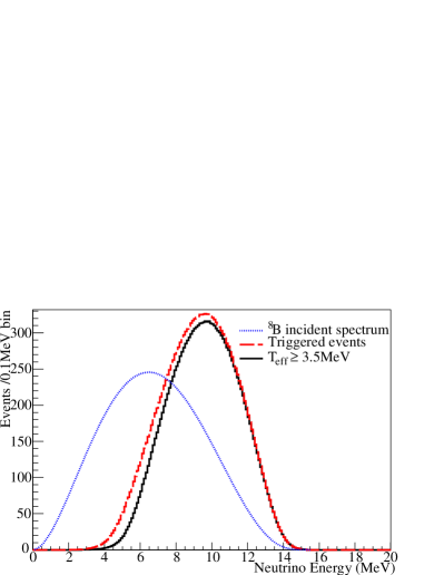
To implement this fit, we performed a ‘four phase’ signal extraction, dividing the data and the PDFs into Phase I-day, Phase I-night, Phase II-day, and Phase II-night groups. Background decay rates from solid media, such as the acrylic vessel and the PMTs, were constrained to be identical day and night. Decay rates in the D₂O and H₂O regions were free to vary between day and night to allow for day/night variations in the water circulation and filtration schedules. We floated the same detector systematics as in the unconstrained fit described in Sec. XIV.3. The fit has 6 neutrino parameters, 26 background normalization parameters, and 16 detector systematic parameters, for a total of 48 free parameters.

We constructed the PDFs in the same way as described in Sec. XIV.3, with the exception of the CC and ES signals. Instead of creating a 3D PDF ($\beta_{14}$, $R^{3}$, $\cos\theta_{\odot}$) for intervals in $T_{\rm eff}$ in the undistorted spectrum, we created 4D PDFs ($T_{\rm eff}$, $\beta_{14}$, $R^{3}$, $\cos\theta_{\odot}$) for separate $E_{\nu}$ intervals in the undistorted spectrum. There were 9 CC and 9 ES PDFs in each of the 4 day/night phases, with $E_{\nu}$ boundaries at $4,6,7,8,9,10,11,12,13,$ and $15$ MeV.

During optimization, the signal rates associated with the 76 CC, ES and NC PDFs were not allowed to vary freely, but were determined by the 6 neutrino parameters. We defined an ‘ES survival probability’:

$$P_{\rm ES}^{\rm day}(E_{\nu}) = P_{ee}^{\rm day}+\epsilon(1-P_{ee}^{\rm day}(E_{\nu}))$$ (25)

$$P_{\rm ES}^{\rm night}(E_{\nu}) = P_{ee}^{\rm night}+\epsilon(1-P_{ee}^{\rm night}(E_{\nu}))$$ (26)

where $\epsilon=0.156$ is the approximate ratio between the $\nu_{\mu,\tau}$ and $\nu_{e}$ ES cross sections. The ES cross-section ratio is not constant as a function of neutrino energy, so we took the variation with energy as an additional systematic uncertainty. The signal rates were defined in terms of $\Phi_{{}^{8}{\rm B}}$, $P_{ee}$ and $P_{\rm ES}$ to be:

$$R_{\mathrm{NC}} = \Phi_{{}^{8}{\rm B}}$$ (27)

$$R_{\mathrm{CC},i}^{\rm day} = \frac{\Phi_{{}^{8}{\rm B}}}{E_{i}-E_{i-1}}\int_{E_{i-1}}^{E_{i}}dE_{\nu}\;P_{ee}^{\rm day}(E_{\nu})$$ (28)

$$R_{\mathrm{CC},i}^{\rm night} = \frac{\Phi_{{}^{8}{\rm B}}}{E_{i}-E_{i-1}}\int_{E_{i-1}}^{E_{i}}dE_{\nu}\;P_{ee}^{\rm night}(E_{\nu})$$ (29)

$$R_{\mathrm{ES},i}^{\rm day} = \frac{\Phi_{{}^{8}{\rm B}}}{E_{i}-E_{i-1}}\int_{E_{i-1}}^{E_{i}}\;dE_{\nu}\;P_{\rm ES}^{\rm day}(E_{\nu})$$ (30)

$$R_{\mathrm{ES},i}^{\rm night} = \frac{\Phi_{{}^{8}{\rm B}}}{E_{i}-E_{i-1}}\int_{E_{i-1}}^{E_{i}}dE_{\nu}\;P_{\rm ES}^{\rm night}(E_{\nu})$$ (31)

where $E_{0}$ is 4 MeV and $E_{i}$ is the upper energy boundary of the $i$-th $E_{\nu}$ interval.

The survival probability fit included the same ‘shift-and-refit’ systematics as the unconstrained fit, along with all of the day/night systematics used in previous analyses longd2o ; nsp . These systematics accounted for diurnal variations in reconstructed quantities, such as energy scale and vertex resolution, as well as long-term variation in detector response which could alias into a day/night asymmetry. In addition, the non-uniformity of the $\cos\theta_{\odot}$ distributions of CC and ES events can also alias into a day/night asymmetry, so we incorporated additional day/night systematic uncertainties on all observables in the CC and ES PDFs.

XIV.5 Application of Constraints

A priori information from calibrations and background measurements was included in the fits to constrain some of the fit parameters, in particular several of the radioactive backgrounds (discussed in Sec. XIII.2) and any systematic parameters floated in the fit.

The extended likelihood function had the form:

$$\mathcal{L}(\vec{\alpha},\vec{\beta})=\mathcal{L}_{data}(\vec{\alpha}|\vec{\beta})\mathcal{L}_{calib}(\vec{\beta})$$ (32)

where $\vec{\alpha}$ represents the set of signal parameters being fit for, $\vec{\beta}$ represents the nuisance parameters for the systematic uncertainties that were floated in the fits, $\mathcal{L}_{data}(\vec{\alpha}|\vec{\beta})$ is the extended likelihood function for the neutrino data given the values of those parameters, and $\mathcal{L}_{calib}(\vec{\beta})$ is a constraint term representing prior information on the systematic parameters, obtained from calibration data and ex-situ measurements. The contribution to $\mathcal{L}_{calib}(\vec{\beta})$ for each systematic parameter had the form:

$$\mathcal{L}_{calib}({\beta_{i}})=e^{\frac{-(\beta_{i}-\mu_{i})^{2}}{2\sigma_{i}^{2}}}$$ (33)

where $x_{i}$ is the value of parameter $i$, and $\mu_{i}$ and $\sigma_{i}$ are the estimated value and uncertainty determined from external measurements (with asymmetric upper and lower values for $\sigma_{i}$ where required). This results in a reduction of the likelihood as the parameter value moves away from the a priori estimate.

XIV.6 Bias Testing

To verify that the signal extraction methods were unbiased, we used half the Monte Carlo events to create ‘fake data’ sets, and the remaining events to create PDFs used in fits to the fake data sets. A fit was performed for each set and the results were averaged to evaluate bias and pull in the fit results.

We created 100 sets containing only neutrino events, 45 sets also containing internal background events, and 15 sets containing the full complement of neutrino events and internal and external backgrounds. The numbers of fake data sets were limited by the available computing resources.

The two signal extraction methods gave results that were in excellent agreement for every set. The biases for the neutrino fluxes were consistent with zero, and the Gaussian pull distributions were consistent with a mean of zero and standard deviation of 1.

Additional tests were performed in which one or more systematic shifts were applied to the event observables in the fake data sets, and the corresponding systematic parameters were floated in the fit, using a priori inputs as in the final signal extraction fits, to verify that the two independent methods for propagating systematic uncertainties were also unbiased. In all cases, the true values for the neutrino fluxes were recovered with biases consistent with zero.

XIV.7 Corrections to PDFs

A number of corrections were required to account for residual differences between data and PDFs derived by simulation. An offset of the laserball position along the $z$-axis during calibration of PMT timing introduced an offset to reconstructed positions along this axis in the data. A correction was therefore applied to all data events, as described in Sec. VI. In addition, a number of corrections were applied to the reconstructed energy and isotropy of events (see Sections VIII.2 and IX, respectively).

The Monte Carlo simulation was used to link the neutrino rates between the two phases, thus taking into account variations in detector efficiency and livetime. Several corrections were applied to the Monte Carlo flux predictions, as described below.

The predicted number of events for signal type $i$ per unit of incident flux, including all correction factors, is:

$$N_{i} = N^{\rm MC}_{i}\,\delta^{\rm sim}\,\delta^{\rm acc}_{i}\,N^{\rm iso}_{i}\,N^{\rm D}_{i}\,N^{e}_{i}\,R_{i}\,\tau,$$ (34)

where:

• $N^{\rm MC}_{i}$ is the number of events predicted by the Monte Carlo simulation for signal $i$ per unit incident flux. This is recalculated as needed to account for any systematic shifts applied to the PDFs.

• $\delta^{\rm sim}$ corrects for events aborted in the simulation due to photon tracking errors. This correction increases with the number of photons in an event.

• $\delta^{\rm acc}_{i}$ corrects for differences in the acceptances of the instrumental and high level cuts for data and Monte Carlo events (Sec. X.5).

• $N^{\rm iso}_{i}$ is a correction to account for CC interactions on chlorine and sodium nuclei in the D₂O volume that are not modeled in the simulation. This correction is relevant only to the CC signal in Phase II.

• $N^{\rm D}_{i}$ is a correction to the number of target deuterons and hence is relevant to CC and NC only.

• $N^{e}_{i}$ is a correction to the number of target electrons and hence is relevant to ES only.

• $R_{i}$ accounts for radiative corrections to the neutrino-deuteron interaction cross section for NC. Radiative corrections relevant to the CC and ES interactions were included in the simulation.

• $\tau$ corrects for deadtime introduced into the data set by the instrumental cuts.

These corrections are summarized in Table 17.

Correction	Phase		CC	ES	NC
$\delta^{\rm sim}$	I, II		(1.0 - 0.0006238$\times T_{\rm eff}$)-1
$\delta^{\rm acc}_{i}$	I		0.9924	0.9924	0.9924
$\delta^{\rm acc}_{i}$	II		0.9930	0.9930	0.9954
$N^{\rm iso}_{i}$	II		1.0002	—	—
$N^{\rm D}_{i}$	I, II		1.0129	—	1.0129
$N^{e}_{i}$	I, II		—	1.0131	—
$R_{i}$	I, II		—	—	0.977
$\tau$	I		0.979	0.979	0.979
$\tau$	II		0.982	0.982	0.982

Table 17: Corrections applied to the expected number of CC, ES and NC events used in the signal extraction fits.

XV Results

The detailed improvements made to this analysis, as described in previous sections, allow a more precise extraction of the neutrino flux parameters and, as a result, of the MSW oscillation parameters. Results from the unconstrained fit are given in Sec. XV.1 and from the energy-dependent fit to the $\nu_{e}$ survival probability in Sec. XV.2. This new method for directly extracting the form of the $\nu_{e}$ survival probability from the signal extraction fit produces results that are straightforward to interpret. A direct comparison can be made of the shape of the extracted survival probability to model predictions, such as the LMA-predicted low-energy rise.

Sec. XV.3 describes the measurements of the neutrino oscillation parameters. As has been observed in a number of recent publications t131 ; t132 ; t133 , the different dependence of the $\nu_{e}$ survival probability on the mixing parameters $\theta_{12}$ and $\theta_{13}$ between solar and reactor neutrino experiments means that a comparison of solar data to reactor antineutrino data from the KamLAND experiment allows a limit to be placed on the value of $\sin^{2}\theta_{13}$. The new precision achieved with the LETA analysis in the measurement of $\tan^{2}\theta_{12}$ results in a better handle on the value of $\sin^{2}\theta_{13}$ in such a three-flavor oscillation analysis. Results of this analysis are presented in Sec. XV.3, including a constraint on the value of $\sin^{2}\theta_{13}$.

XV.1 Unconstrained Fit

Our measurement of the total flux of active ⁸B solar neutrinos, using the NC reaction ($\Phi_{\textrm{NC}}$) is found to be:

• Binned-histogram method

$\Phi_{\textrm{NC}}^{binned}=5.140\,^{+0.160}_{-0.158}\textrm{(stat)}\,^{+0.132}_{-0.117}\textrm{(syst)}\times 10^{6}\,\rm cm^{-2}\,s^{-1}$

• Kernel estimation method

$\Phi_{\textrm{NC}}^{kernel}=5.171\,^{+0.159}_{-0.158}\textrm{(stat)}\,^{+0.132}_{-0.114}\textrm{(syst)}\times 10^{6}\,\rm cm^{-2}\,s^{-1}$

This represents ${}^{+4.0}_{-3.8}$% total uncertainty on the flux, which is more than a factor of two smaller than the best of previous SNO results. The statistical uncertainty has been reduced by nearly $\sqrt{2}$, to 3.1%. However, the largest improvement is in the magnitude of the systematic uncertainty, which has been reduced from 7.3% and 6.3% in previous analyses of Phase II nsp and Phase III snoncd data, respectively, to 2.4% (taking the average of the upper and lower values).

Figure 27 shows a comparison of these results to those from previous analyses of SNO data. Note that the ⁸B spectral shape used in the previous Phase I and Phase II analyses oldb8spec differs from that used here winter . The bands represent the size of the systematic uncertainties on each measurement, thus illustrating the improvements achieved with this analysis.

Figure 27: (Color online) Total ⁸B neutrino flux results using the NC reaction from both unconstrained signal extraction fits in comparison to unconstrained fit results from previous SNO analyses. ‘LETA I’ refers to the binned-histogram method and ‘LETA II’ to the kernel estimation method.

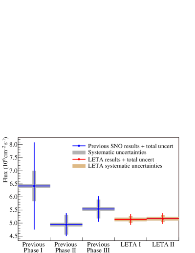
Throughout this analysis, the quoted ‘statistical’ uncertainties represent the uncertainty due to statistics of all signals and backgrounds in the fit, with correlations between event types taken into account. Therefore, they include uncertainties in the separation of signal events from backgrounds in the fits. For example, the statistical uncertainties on the quoted results for $\Phi_{\textrm{NC}}$ include both the Poisson uncertainty in the number of NC events, and covariances with other event types. This is different from previous SNO analyses, in which the background events were not included in the signal extraction fits and any uncertainty in the level of background events was propagated as an additional systematic uncertainty.

The two independent signal extraction fit techniques are in excellent agreement, both in the central NC flux value and in the magnitude of the uncertainties. The result from the binned-histogram method is quoted as the final unconstrained fit result for ease of comparison to previous analyses, which used a similar method for PDF creation.

This result is in good agreement with the prediction from the BS05(OP) SSM of 5.69$\times 10^{6}\,\rm cm^{-2}\,s^{-1}$ bs05 , to within the theoretical uncertainty of $\pm 16$%. It is also in good agreement with the BS05(AGS,OP) model prediction of 4.51$\times 10^{6}\,\rm cm^{-2}\,s^{-1}\pm 16$% bs05 , which was constructed assuming a lower heavy-element abundance in the Sun’s surface.

The extracted CC and ES electron spectra from both signal extraction fits, in terms of the fraction of one unoscillated SSM, using the BS05(OP) model flux of 5.69$\times 10^{6}\,\rm cm^{-2}\,s^{-1}$ bs05 , are shown in Figure 28. An unsuppressed, undistorted spectrum would correspond to a flat line at 1.0. A greater suppression is observed for CC events than ES, since the ES spectrum includes some contribution from $\nu_{\mu}$ and $\nu_{\tau}$ whereas CC is sensitive only to $\nu_{e}$. Both spectra are consistent with the hypothesis of no distortion. The results from the two independent signal extraction fits are again in excellent agreement for both the central fit values and the uncertainties.

Figure 28: (Color online) Extracted a) CC and b) ES electron spectra as a fraction of one unoscillated SSM (BS05(OP)), from both signal extraction fits, with total uncertainties. The final 12–20 MeV bin in the kernel estimation fit is plotted at the mean of the spectrum in that range. Both spectra are consistent with the hypothesis of no distortion (a flat line).

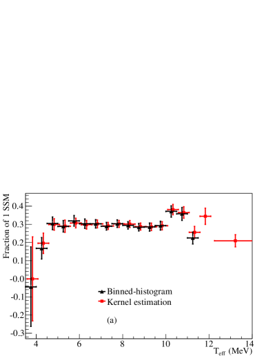
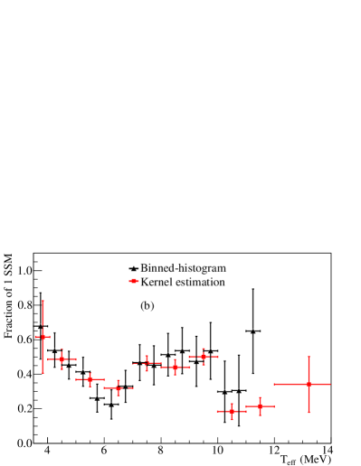
Figure 29 shows the CC electron spectrum extracted from the binned-histogram signal extraction fit with the errors separated into the contributions from statistical and systematic uncertainties. As for the NC flux result, the uncertainties are dominated by those due to statistics (which includes the ability to distinguish signal from background). This demonstrates the effect of the significant improvements made both in the determination of the individual systematic uncertainties, as presented in previous sections, and in the improved treatment of the dominant systematic uncertainties, whereby the self-consistency of the data itself was used to further constrain the allowed ranges of these parameters. It is worth noting that correlations between bins, which are not shown, tend to reduce the significance of any observed shape. Fitting to an undistorted spectrum (the flat line on Fig. 29) gives a $\chi^{2}$ value of 21.52 for 15 degrees of freedom, which is consistent with the hypothesis of no distortion. The prediction for the $T_{\rm eff}$ spectrum for CC events taken from the best fit LMA point from a previous global analysis of solar data snoncd is also overlaid on Fig. 29. The $\chi^{2}$ value of the fit of the extracted spectrum to this prediction is 22.56 for 15 degrees of freedom, demonstrating that the data are also consistent with the LMA prediction.

Figure 29: (Color online) Extracted CC electron spectrum as a fraction of one unoscillated SSM (BS05(OP)) from the binned-histogram signal extraction fit, with the uncertainties separated into statistical (blue bars) and systematic (red band) contributions. The predictions for an undistorted spectrum, and for the LMA point $\Delta m^{2}_{21}=7.59\times 10^{-5}\,{\rm eV}^{2}$ and $\tan^{2}\theta_{12}=0.468$ (taken from a previous global solar+KamLAND fit snoncd and floating the ⁸B flux scale) are overlaid for comparison.

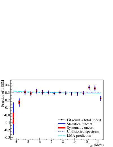
The one-dimensional projections of the fits in each observable parameter from the binned-histogram signal extraction are shown for each phase in Figures 30 and 31. Of particular note is the clear ES peak observed in the $\cos\theta_{\odot}$ fits for both phases (Figs. 30(c) and 31(c)), demonstrating the extraction of ES events over the integrated energy spectrum, even with the low 3.5 MeV threshold. The error bars represent statistical uncertainties; systematic uncertainties are not shown. Figure 32 shows the one-dimensional projection in $T_{\rm eff}$ from Phase II (as in Fig. 31(a)) but with the fitted contributions from individual signal types separated into six categories: CC, ES, and NC neutrino events, internal backgrounds (within the D₂O volume), external backgrounds (in the AV, H₂O, and PMTs) and hep neutrino events.

Figure 30: (Color online) One dimensional projections of the fit in each observable parameter in Phase I, from the binned-histogram signal extraction. The panels show the fit projected onto (a) energy ($T_{\rm eff}$), (b) radius cubed ($R^{3}$), (c) direction ($\cos\theta_{\odot}$), and (d) isotropy ($\beta_{14}$).

Figure 31: (Color online) One dimensional projections of the fit in each observable parameter in Phase II, from the binned-histogram signal extraction. The panels show the fit projected onto (a) energy ($T_{\rm eff}$), (b) radius cubed ($R^{3}$), (c) direction ($\cos\theta_{\odot}$), and (d) isotropy ($\beta_{14}$).

Figure 32: (Color) One dimensional projection of the fit in $T_{\rm eff}$ in Phase II from the binned-histogram signal extraction, with the individual signals separated into the three neutrino interactions, internal backgrounds (within the D₂O volume), external backgrounds (in the AV, H₂O, and PMTs) and hep neutrino events.

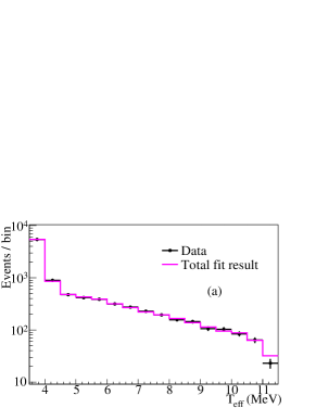
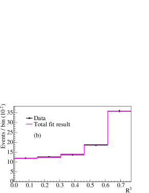
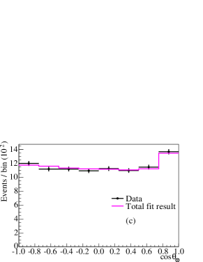
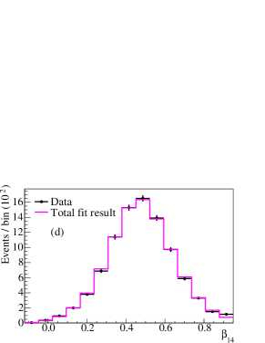
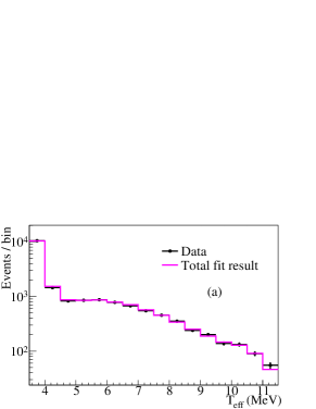
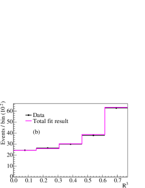
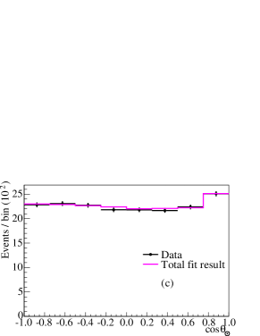
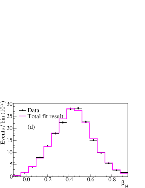
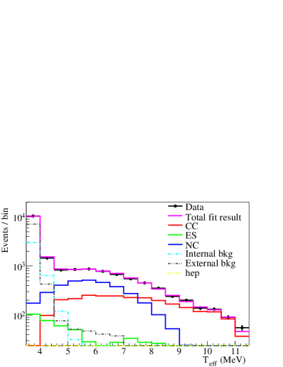
The $\chi^{2}$ for the one-dimensional projections of the fit are given in Table 18. These were evaluated using statistical uncertainties only and are, therefore, a conservative test of goodness-of-fit in the one-dimensional projections. In all dimensions, the final result is a good fit to the data.

Phase	Observable			$\chi^{2}$ (data points)
I	$T_{\rm eff}$			8.17 (16)
	$\cos\theta_{\odot}$			3.69 (8)
	$\rho$			2.61 (5)
	$\beta_{14}$			20.99 (15)
II	$T_{\rm eff}$			13.64 (16)
	$\cos\theta_{\odot}$			3.07 (8)
	$\rho$			2.98 (5)
	$\beta_{14}$			26.25 (15)

Table 18: $\chi^{2}$ values for the fit of the extracted signals from the binned-histogram signal extraction to the data set for one-dimensional projections in each of the four observables, in each phase. These were evaluated using statistical uncertainties only. The number of data points used for the $\chi^{2}$ calculations are given afterwards in parentheses. Because these are one-dimensional projections of a fit in four observables, the probability of obtaining these $\chi^{2}$ values cannot be simply evaluated; these are simply quoted as a qualitative demonstration of goodness-of-fit.

Table 22 in Appendix A shows the extracted number of events for the neutrino fit parameters from the binned-histogram signal extraction fit, with total statistical plus systematic uncertainties.

Table 19 shows the total number of background events extracted by each signal extraction in each phase, and a breakdown of the number of background neutron events occurring within each region of the detector. The two methods are in good agreement based on expectations from studies of Monte Carlo-generated ‘fake’ data sets. For comparison, the total number of events in each data set is also given (taken from Table 6). Due to the exponential shape of the energy spectra of most sources of background in this fit, the majority of the background events fit out in the lowest two bins in $T_{\rm eff}$, illustrating one of the major challenges of the low energy analysis.

	Phase I		Phase II
Background	LETA I	LETA II	LETA I	LETA II
Total background events	6148.9	6129.8	11735.0	11724.6
D2O neutrons	29.7	34.0	122.4	133.5
AV neutrons	214.9	191.4	295.7	303.4
H2O neutrons	9.9	8.4	27.7	26.3
Total data events	9337		18228

Table 19: Number of background events extracted from the signal extraction fits for each method. ‘LETA I’ refers to the binned-histogram signal extraction, and ‘LETA II’ refers to the kernel estimation method. The total number of events in each data set is also given, taken from Table 6.

Tables 23–24 in Appendix A show the effects of the individual systematic uncertainties on the extracted NC rate, the CC rate in two energy intervals (4.0–4.5 MeV and 9.5–10.0 MeV) and the ES rate in the 3.5–4.0 MeV interval, all taken from the binned-histogram fit. The dominant source of uncertainty on the total neutrino flux measured with the NC reaction is the neutron capture uncertainty. Further significant contributions come from the Phase II energy resolution, the $\beta_{14}$ scale for neutron capture events, the energy-dependent fiducial volume, and the cut-acceptance uncertainties.

Figure 33 shows the effects of several groups of systematic uncertainties on the extracted CC electron spectrum, taken from the binned-histogram fit. Four groups cover systematic effects that apply to the observables ($T_{\rm eff}$, $\cos\theta_{\odot}$, $R^{3}$ and $\beta_{14}$), in which the individual contributions are summed in quadrature (for example the $T_{\rm eff}$ group includes the effect of energy scale, resolution and linearity); ‘normalization’ uncertainties include neutron capture, cut-acceptance, energy-dependent fiducial volume and photodisintegration uncertainties; the final group consists of uncertainties in the shape of the PMT $\beta$-$\gamma$ PDF. The dominant sources of the systematic uncertainties on the shape of the CC electron spectrum are energy resolution and the shape of the PMT $\beta$-$\gamma$ PDF, particularly as a function of $T_{\rm eff}$. The $\beta_{14}$ scale for electron-like events is also a significant contributor. It is worth noting that the contribution from the fiducial volume uncertainty, which was significant in previous analyses nsp , is now relatively small.

Figure 33: (Color) Effect of systematic uncertainties on the extracted CC electron spectrum. The inset shows the same plot on a larger scale.

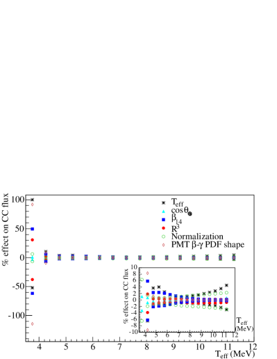
The two signal extraction methods are in excellent agreement for all the neutrino flux parameters, as well as the sources of background events. This is a stringent test of the result, since the two methods differed in several fundamental ways:

• Formation of the PDFs

  The methods used to create the PDFs were entirely independent: one using binned histograms, and the other using smooth, analytic, kernel-estimated PDFs.

• Treatment of systematic uncertainties

  The dominant systematics in the fits were ‘floated’ using different approaches: in the kernel method they were floated directly, whereas an iterative likelihood scan was used in the binned-histogram approach.

• PMT $\beta$-$\gamma$ constraint

  In the binned-histogram method, a constraint on the total number of PMT events was implemented using a bifurcated analysis of the data (Sec. XIII.3), whereas no constraint was applied in the kernel method.

That these independent approaches give such similar results demonstrates the robust nature of the analysis and the final results.

XV.2 Survival Probability Fit

Under the assumption of unitarity (for example, no oscillations between active and sterile neutrinos), the NC, CC, and ES rates can be directly related. Based on this premise, a signal extraction fit was performed in which the free parameters directly described the total ⁸B neutrino flux and the $\nu_{e}$ survival probability. This fit therefore produces a measure of the total flux of ⁸B neutrinos that naturally includes information from all three interaction types. Applying this approach, the uncertainty on the flux was reduced in comparison to that from the unconstrained fit (Sec. XV.1). The total flux measured in this way ($\Phi_{{}^{8}{\rm B}}$) is found to be:

$$\Phi_{{}^{8}{\rm B}}=5.046\,^{+0.159}_{-0.152}\textrm{(stat)}\,^{+0.107}_{-0.123}\textrm{(syst)}\times 10^{6}\,\rm cm^{-2}\,s^{-1},$$

which represents ${}^{+3.8}_{-3.9}$% total uncertainty. This is the most precise measurement of the total flux of ⁸B neutrinos from the Sun ever reported.

The survival probability was parameterized as a quadratic function in $E_{\nu}$, representing $P_{ee}^{\rm day}$, and a linear day/night asymmetry, as defined in Eqs. (22) and (23) of Sec. XIV.4. The best-fit polynomial parameter values and uncertainties are shown in Table 26, and the correlation matrix is shown in Table 27, both presented in Appendix A. For all the extracted parameters, the total uncertainty is dominated by that due to statistics.

Figure 34 shows the RMS spread in the best fit survival probabilities, $P_{ee}^{\rm day}(E_{\nu})$ and $P_{ee}^{\rm night}(E_{\nu})$, and day/night asymmetry, $A(E_{\nu})$. The bands were computed by sampling the parameter space 1000 times, taking into account the parameter uncertainties and correlations. Overlaid on Fig. 34 are the predicted shapes of the day and night survival probabilities and the day/night asymmetry for the best-fit point from a previous global analysis of solar data snoncd .

The advantage of this direct parameterization for the survival probability is that model testing becomes straightforward. We can test the goodness-of-fit to an undistorted spectrum by setting $c_{1}=c_{2}=0.0$ in Eq. 23, and we can test the goodness-of-fit to a model with no day/night asymmetry by setting $a_{0}=a_{1}=0.0$ in Eq. 22. Requiring both simultaneously, we find a $\Delta\chi^{2}=1.94$ for 4 degrees of freedom, demonstrating that the extracted survival probabilities and day/night asymmetry are consistent with the hypothesis of no spectral distortion and no day/night asymmetry. For comparison, the $\Delta\chi^{2}$ value of the fit to the LMA point shown in Fig. 34 is 3.9 for 4 degrees of freedom, showing that the data are also consistent with LMA.

Figure 34: (Color online) Best fit and RMS spread in the (a) $P_{ee}^{\rm day}(E_{\nu})$, (b) $P_{ee}^{\rm night}(E_{\nu})$, and (c) $A(E_{\nu})$ functions. The survival probabilities and day/night asymmetry for the LMA point $\Delta m^{2}_{21}=7.59\times 10^{-5}\,{\rm eV}^{2}$ and $\tan^{2}\theta_{12}=0.468$, taken from a previous global solar+KamLAND fit snoncd , are shown for comparison.

Figure 35: (Color online) One dimensional projections of the fit in Phase I-day, from the polynomial survival probability fit. The panels show the fit projected onto (a) energy ($T_{\rm eff}$), (b) radius cubed ($R^{3}$), (c) direction ($\cos\theta_{\odot}$), and (d) isotropy ($\beta_{14}$). The binning of data is purely for display purposes; the fits were performed unbinned.

Figure 36: (Color online) One dimensional projections of the fit in Phase II-night, from the polynomial survival probability fit. The panels show the fit projected onto (a) energy ($T_{\rm eff}$), (b) radius cubed ($R^{3}$), (c) direction ($\cos\theta_{\odot}$), and (d) isotropy ($\beta_{14}$). The binning of data is purely for display purposes; the fits were performed unbinned.

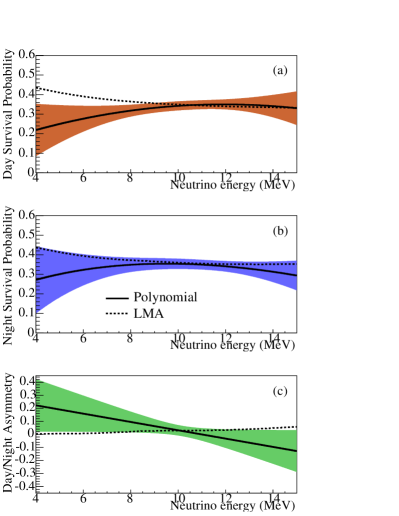
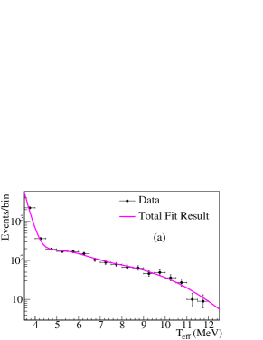
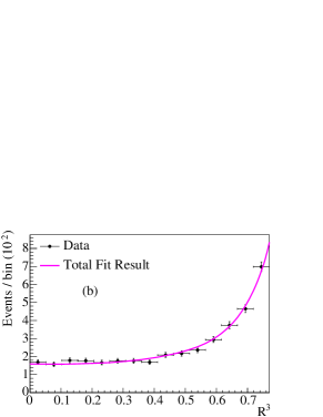
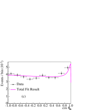
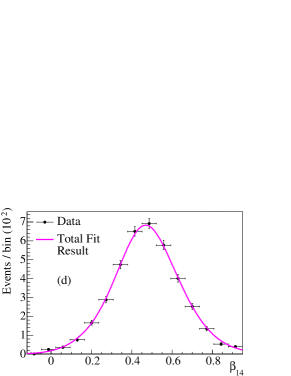
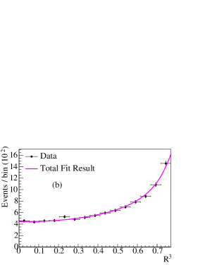
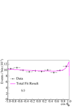
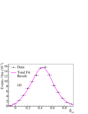
This method for parameterizing the day/night asymmetry differs from previous SNO analyses, which quoted an asymmetry for each interaction type:

$$A=2\frac{(\phi_{N}-\phi_{D})}{(\phi_{N}+\phi_{D})},$$ (35)

where $\phi_{D}$ and $\phi_{N}$ are the interaction rates measured for the day and night data sets, respectively. A combined analysis of the results from Phase I and Phase II, assuming an undistorted neutrino spectrum, gave a result of $A=0.037\pm 0.040$ nsp . For comparison, the current analysis made no assumption about the shape of the underlying neutrino spectrum, except that it is a smooth, slowly varying function of $E_{\nu}$ over the range of neutrino energies to which the SNO detector is sensitive. The value of $a_{0}$ extracted under this assumption was $a_{0}=0.032\pm 0.040$. Uncertainty on the day/night asymmetry measurement has always been dominated by statistics, so the improvements made to systematic uncertainties in this analysis have a small effect. The effect of the additional statistics gained by going lower in energy appears to be balanced by the additional degrees of freedom allowed in the shape of the neutrino energy spectrum.

The one-dimensional projections of the fits in the observable parameters for Phase I-day and Phase II-night are shown in Figures 35 and 36.

XV.3 Mixing Parameters

A three-flavor, active solar neutrino oscillation model has four parameters: $\theta_{12}$ and $\theta_{13}$, which quantify the strength of the mixing between flavor and mass eigenstates, and $\Delta m^{2}_{21}$ and $\Delta m^{2}_{31}$, the differences between the squares of the masses of the neutrino propagation eigenstates. The approximation of $\Delta m^{2}_{31}\sim\Delta m^{2}_{32}$ can be made because $|\Delta m^{2}_{32}|\gg|\Delta m^{2}_{21}|$, while the remaining mixing angle, $\theta_{23}$, and the CP-violating phase, $\delta$, are irrelevant for the oscillation analysis of solar neutrino data.

For the sake of comparison with other oscillation analyses, this work employed $\tan^{2}\theta_{12}$ to quantify the leading effects of the mixing angles for solar neutrino oscillations. Smaller effects due to $\theta_{13}$ are quantified with $\sin^{2}\theta_{13}$. The value of $\Delta m^{2}_{31}$ was fixed to $+2.3\times 10^{-3}\ \mathrm{eV^{2}}$ pdg08 , an assumption that was necessary for the numerical determination of the three-flavor survival probabilities, but whose precise value had very little impact on our calculation.

The parameters describing the $P_{ee}(E_{\nu})$ function for solar neutrinos are, in order of importance, $\theta_{12}$, $\Delta m^{2}_{21}$, $\theta_{13}$, and $\Delta m^{2}_{31}$. For experiments sensitive to neutrinos from terrestrial sources, near the detector, the survival probabilities were accurately calculated using a formula without the effect of matter. The inclusion of matter effects in the survival probability calculation for solar neutrino experiments involves the numerical integration of a system of coupled differential equations:

$$i\,\frac{d}{dx}\psi_{\alpha}(x)=H_{f}\,\psi_{\alpha}(x)\,,$$ (36)

where $H_{f}$ is the Hamiltonian in flavor space, including matter effects in both the Sun and the Earth, $x$ is the position along the propagation direction, and $\psi_{\alpha}(x)$ is a vector containing the real and imaginary coefficients of the wave function, where $\alpha=$ (e, $\mu$, $\tau$). The system was solved for each new value of $x$ as the wave function was propagated from the Sun to a given detector on the Earth. The probabilities were then calculated from the magnitudes of the wave function coefficients. The integration was performed with the adaptative Runge-Kutta algorithm. Radial profiles of the electron density and neutrino production in the Sun were taken from the BS05(OP) model bs05 . The matter density inside the Earth was taken from the Preliminary Reference Earth Model (PREM) prem , which is the most widely accepted data since the density profile is inferred from seismological considerations. For more details on the survival probability calculation, see olivier .

Constraints on neutrino mixing parameters can be derived by comparing neutrino oscillation model predictions with experimental data, as has been done in previous SNO analyses longd2o ; nsp ; snoncd . The approach for the interpretation of the solar and reactor neutrino data used the covariance $\chi^{2}$ method. From a series of observables with an associated set of measured parameters from a number of experiments, the corresponding theoretical expectations were calculated for a given neutrino oscillation parameter hypothesis. In order to calculate the model prediction for the neutrino yield at a given detector, each of the neutrino fluxes that the detector was sensitive to was weighted with the neutrino survival probabilities, convolved with the cross-sections for the neutrino-target interactions as well as with the detector response function, and then considered above the experiment’s energy threshold. The $\chi^{2}$ function quantifies the difference between the experimental data and theoretical model expectation for the observable under study.

In the results presented here, the free parameters were the neutrino mixing parameters and the total flux of the ⁸B and hep neutrinos. The survival probabilities and, hence, the fluxes and spectra of solar neutrinos and reactor antineutrinos were fully constrained by the mixing parameters. The $\chi^{2}$ function in each case was minimized over a fine grid of points with respect to $\tan^{2}\theta_{12}$, $\sin^{2}\theta_{13}$, and $\Delta m^{2}_{21}$. The $\Delta\chi^{2}=\chi^{2}-\chi^{2}_{\rm{min}}$ differences were the indicators of the confidence levels (C.L.) in the one- and two-dimensional projections. The 68%, 95%, and 99.78% C.L. regions in two-dimensional parameter projections were drawn following the standard definitions: $\Delta\chi^{2}=$ 2.279, 5.99, and 11.83, respectively. For one-dimensional projections the errors on the parameter were the standard $1\sigma$ C.L. at $\Delta\chi^{2}=1$. For all projections shown in this section, the $\chi^{2}$ was minimized with respect to the undisplayed parameters at each point in the MSW space.

The information from the LETA survival probability measurement was included by evaluating the polynomial survival probability and day/night asymmetry (as defined in Eqs. (22) and (23) of Sec. XIV.4) that best represented the model prediction at each point in the MSW plane. To do this, it was necessary to take into account the sensitivity of the SNO detector (including effects such as the energy dependence of the cross sections, reaction thresholds, and analysis cuts) so that the parameterization of the model prediction at each point in the MSW plane sampled the neutrino energy spectrum in the same manner and over the same range as the data. We calculated the number of detected events that passed all the cuts as a function of neutrino energy using the Monte Carlo simulation, and what was thus equivalent to a ‘detected neutrino energy spectrum’ (given in Table 28 in Appendix A) was distorted by the model-predicted survival probability at each point in the MSW plane. This was fit to a similarly obtained spectrum, now distorted by the polynomial parameterization, allowing the five polynomial parameters to vary in the fit. At each point in the plane, we then calculated the $\chi^{2}$ value of the fit of the model-predicted polynomial parameters ($c_{0}$, $c_{1}$, $c_{2}$, $a_{0}$, and $a_{1}$) to the result from the signal extraction, taking into account all uncertainties and correlations as output by the signal extraction fit. The SNO rates from Phase III snoncd were treated as a separate data set.

Figure 37 shows the allowed regions of the $(\tan^{2}\theta_{12},\Delta m^{2}_{21})$ parameter space when the LETA data were analyzed in combination with the rates from Phase III snoncd . The $2\nu$ contours were projected from the parameter space at a constant value of $\sin^{2}\theta_{13}=0.0$, making them equivalent to an effective two-flavor analysis. While the best fit point falls in the so-called ‘LOW’ region, with $\Delta m^{2}_{21}=1.15\,^{+0.38}_{-0.18}\times 10\,^{-7}(\mathrm{eV}^{2})$ and $\tan^{2}\theta_{12}=0.437\,^{+0.058}_{-0.058}$, the significance levels of the LOW and the higher mass Large Mixing Angle (LMA) regions are very similar. The predicted shape for the survival probability is very flat in both regions, and the day/night asymmetry is expected to be small, so the SNO-only analysis has little handle on distinguishing the two regions. A notable difference between LOW and LMA is in the predicted sign of the slope of the energy dependence of the day/night asymmetry, with LOW predicting a negative slope, as was extracted in the polynomial survival probability signal extraction fit reported in Sec. XV.2.

Figure 37: (Color) SNO (LETA + Phase III) two-flavor oscillation parameter analysis.

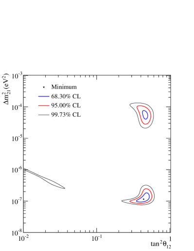
As described above, the observables from the SNO LETA fit used in the hypothesis testing were the polynomial parameters of the survival probability. In a full global analysis, event yields were used for the other solar neutrino experiments, including the SNO Phase III results. For each set of parameters, the oscillation model was used to predict the rates in the Chlorine home2 , Gallium sage , and Borexino bor experiments, the Super-Kamiokande Phase I zenith spectra sk1 and Phase II day/night spectra sksol , and the KamLAND rates and spectrum kam , as well as the SNO rates snoncd and spectra. The expected rates and spectra were divided by the respective predictions, calculated without oscillations, to remove the effects of the model scaling factors. The unitless rates were then used in the global $\chi^{2}$ calculation.

Although the $\Phi_{{}^{8}{\rm B}}$ scale was determined in the LETA signal extraction, we re-introduced it as a free parameter in the $\chi^{2}$ minimization at each point in the parameter space to constrain it with all solar data. The uncertainty of the scale was retrieved from its marginal distribution, as was done for the oscillation parameters.

The SNO LETA covariance matrix was taken from the signal extraction output given in Table 27, as before. For other experiments, the total covariance matrix was assembled from the individual statistical and systematic components, as described in nsp . Correlations between SNO’s LETA and other solar experimental results were allowed via the floated $\Phi_{{}^{8}{\rm B}}$ scale parameter.

The KamLAND rates and spectrum were predicted using three-flavor vacuum oscillations. Publicly available information about the KamLAND detector and nearby reactors were included in our calculation, which reproduced the unoscillated spectrum of Fig. 1 of Ref. kam with good accuracy. To include the effects of three-flavor oscillations, we then compared the $\chi^{2}$ obtained with non-zero values of $\theta_{13}$ with those obtained with $\theta_{13}=0$, for each set of ($\tan^{2}\theta_{12}$, $\Delta m^{2}_{21}$) values. In this way, we built a $\Delta\chi^{2}$ function to parameterize the change of the $\chi^{2}$ map in Fig. 2 of Ref. kam due to a non-zero value of $\theta_{13}$. This allowed us to include the KamLAND experiment in our three-flavor neutrino oscillation analysis and to precisely reproduce KamLAND’s two-flavor neutrino contours. When including the KamLAND antineutrino spectrum we assumed CPT invariance, and we used the KamLAND data only to constrain the oscillation parameters (as opposed to the ⁸B flux scale), whereas all other solar neutrino rates were used to collectively determine the absolute scale of the ${}^{8}\mathrm{B}$ neutrino flux as well as the oscillation parameters.

Figure 38 shows the allowed regions of the $(\tan^{2}\theta_{12},\Delta m^{2}_{21})$ parameter space when the global solar data and the KamLAND data were analyzed, both separately and together, in a two-flavor analysis. It is interesting to note that the global solar analysis does not significantly alter the constraints in the LMA region relative to the SNO-only analysis.

Figure 38: (Color) Two-flavor oscillation parameter analysis for a) global solar data and b) global solar + KamLAND data. The solar data includes: SNO’s LETA survival probability day/night curves; SNO Phase III integral rates; Cl; SAGE; Gallex/GNO; Borexino; SK-I zenith and SK-II day/night spectra.

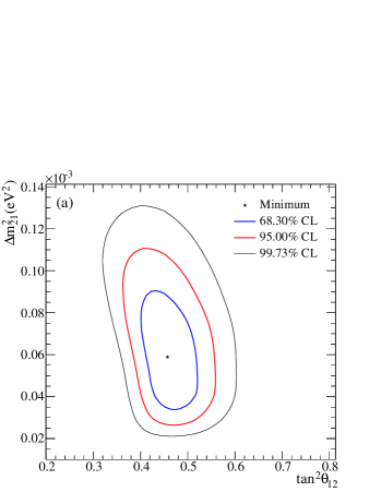
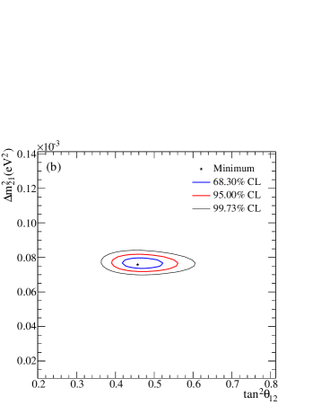
Figure 39 shows the results of a three-flavor oscillation analysis. Fig. 39(a) shows an overlay of the global solar and the KamLAND allowed regions in $(\tan^{2}\theta_{12},\Delta m^{2}_{21})$ parameter space, under a two-flavor hypothesis. Fig. 39(b) shows the same overlay for the three-flavor hypothesis. Allowing the value of $\sin^{2}\theta_{13}$ to be non-zero clearly brings the two regions into much better agreement. The three-flavor contours show the effect of allowing both $\Phi_{{}^{8}{\rm B}}$ and $\sin^{2}\theta_{13}$ to float at each point in space. Allowing these extra degrees of freedom worsens the uncertainties on the two dominant oscillation parameters, $\tan^{2}\theta_{12}$ and $\Delta m^{2}_{21}$. The regions obtained with all solar data are consistent with the SNO-only data and show an extension of the space towards larger values of $\tan^{2}\theta_{12}$ when $\sin^{2}\theta_{13}$ is allowed to vary. In contrast, the three-flavor KamLAND contours show an extension towards smaller values of $\tan^{2}\theta_{12}$.

Figure 39: (Color) Solar and KamLAND oscillation parameter analysis for a) a two-flavor oscillation hypothesis and b) a three-flavor hypothesis. The solar data includes SNO’s LETA survival probability day/night curves, SNO Phase III integral rates, Cl, SAGE, Gallex/GNO, Borexino, SK-I zenith and SK-II day/night spectra. The $\chi^{2}$ is minimized with respect to all undisplayed parameters, including $\sin^{2}\theta_{13}$ and $\Phi_{{}^{8}{\rm B}}$.

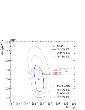
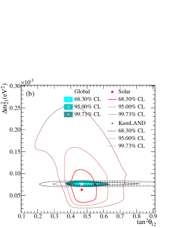
Figure 40 shows the confidence regions in the $(\tan^{2}\theta_{12},\sin^{2}\theta_{13})$ space. The directionality of the contours explains the excellent agreement of $\tan^{2}\theta_{12}$ between the solar and KamLAND experiments when $\sin^{2}\theta_{13}$ is allowed to vary in the fit.

Figure 40: (Color) Solar oscillation parameter analysis, identical to Fig. 39(b), but projected in the mixing angle space. The $\chi^{2}$ is minimized with respect to all undisplayed parameters, including $\Delta m^{2}_{21}$ and $\Phi_{{}^{8}{\rm B}}$.

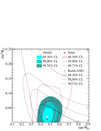
Tables 20 and 21 summarize the oscillation parameter results from the various two- and three-flavor oscillation analyses, respectively. When all solar experiments are combined with data from the KamLAND reactor antineutrino experiment in a two-flavor fit, the best fit point is found to be at $\theta_{12}=34.06\,^{+1.16}_{-0.84}$ degrees and $\Delta m^{2}_{21}=7.59\,^{+0.20}_{-0.21}\times 10^{-5}$ eV². The uncertainty on the mixing angle has been noticeably reduced in comparison to SNO’s previous analyses, resulting in the world’s best measurement of $\theta_{12}$ to date. The global value of $\Phi_{{}^{8}{\rm B}}$ from this fit is extracted to a precision of ${}^{+2.38}_{-2.95}$%. The combination with KamLAND in a three-flavor fit has allowed us to constrain $\sin^{2}\theta_{13}$, giving a value of $\sin^{2}\theta_{13}=2.00^{+2.09}_{-1.63}\times 10^{-2}$. This implies an upper bound of $\sin^{2}\theta_{13}<0.057$ (95% C.L.).

Oscillation analysis	$\tan^{2}\theta_{12}$	$\Delta m^{2}_{21}(\mathrm{eV}^{2})$
SNO (LOW)	$0.437\,^{+0.058}_{-0.058}$	$1.15\,^{+0.38}_{-0.18}\times 10\,^{-7}$
SNO (LMA)	$0.457\,^{+0.038}_{-0.042}$	$5.50\,^{+2.21}_{-1.62}\times 10\,^{-5}$
Solar	$0.457\,^{+0.038}_{-0.041}$	$5.89\,^{+2.13}_{-2.16}\times 10\,^{-5}$
Solar+KamLAND	$0.457\,^{+0.040}_{-0.029}$	$7.59\,^{+0.20}_{-0.21}\times 10\,^{-5}$
	$\chi^{2}_{\mathrm{min}}/\mathrm{ndf}$	$\Phi_{{}^{8}{\rm B}}$ ($\times 10^{6}\,\rm cm^{-2}\,s^{-1}$)
SNO (LOW)	$6.80/9$	$5.013\,^{+0.176}_{-0.199}$
SNO (LMA)	$8.20/9$	$4.984\,^{+0.205}_{-0.182}$
Solar	$67.5/89$	$5.104\,^{+0.199}_{-0.148}$
Solar+KamLAND	$82.8/106$	$5.013\,^{+0.119}_{-0.148}$

Table 20: Best-fit neutrino oscillation parameters and extracted ⁸B flux from a two-flavor oscillation analysis. The ‘SNO’ results are from the combined LETA + Phase III oscillation analysis. Uncertainties listed are $\pm 1\sigma$ after the $\chi^{2}$ was minimized with respect to all other parameters.

Oscillation analysis	$\tan^{2}\theta_{12}$	$\Delta m^{2}_{21}(\mathrm{eV}^{2})$
Solar	$0.468\,^{+0.052}_{-0.050}$	$6.31\,^{+2.49}_{-2.58}\times 10\,^{-5}$
Solar+KamLAND	$0.468\,^{+0.042}_{-0.033}$	$7.59\,^{+0.21}_{-0.21}\times 10\,^{-5}$
	$\chi^{2}_{\mathrm{min}}/\mathrm{ndf}$	$\Phi_{{}^{8}{\rm B}}$ ($\times 10^{6}\,\rm cm^{-2}\,s^{-1}$)
Solar	$67.4/89$	$5.115\,^{+0.159}_{-0.193}$
Solar+KamLAND	$81.4/106$	$5.087\,^{+0.171}_{-0.159}$
	$\sin^{2}\theta_{13}(\times 10\,^{-2})$
Solar	$<8.10\,(95\%\,{\rm\,C.L.)}$
Solar+KamLAND	$2.00\,^{+2.09}_{-1.63}$

Table 21: Best-fit neutrino oscillation parameters and extracted ⁸B flux from a three-flavor oscillation analysis. Uncertainties listed are $\pm 1\sigma$ after the $\chi^{2}$ was minimized with respect to all other parameters.

XVI Summary and Conclusions

We have described here a joint low energy threshold analysis of SNO’s Phase I and Phase II data sets down to an effective kinetic energy threshold of $T_{\rm eff}=3.5$ MeV. The low threshold increased the statistics of the CC and ES events by roughly 30%, and of NC events by $\sim$70%. A new energy estimator improved the energy resolution by 6%, thus reducing the number of background events reconstructing above threshold by $\sim$60%. Separation of electron-like and neutron capture events was improved by the joint fit of data from Phases I and II, due to the difference in neutron detection sensitivity in the two phases. In addition, use of calibration data to correct the Monte Carlo-generated PDF shapes, and reduction of systematic uncertainties, have all contributed to increased precision on both the total ⁸B solar neutrino flux and the derived neutrino mixing parameters. Fitting our data without constraints on the shape of the underlying neutrino energy spectrum or the unitarity of the mixing matrix gives a total ⁸B neutrino flux of $\phi_{\rm NC}=5.14^{+0.21}_{-0.20}\mbox{\,(stat\,$\oplus$\,syst)}\times 10^{6}$cm^-2 s^-1, measured by the NC reaction only, where $\oplus$ refers to the quadrature sum. This is in good agreement with the predictions of recent Standard Solar Models. The uncertainties on this result are more than a factor of two better than in our previous publications. The CC and ES reconstructed electron spectra for this fit are consistent with the hypothesis of no spectral distortion, and with the best fit LMA point.

We have also used the unique capabilities of the SNO detector to perform the first direct fit to data for the energy-dependent $\nu_{e}$ survival probability, without any reference to flux models or other experiments. The fit for the survival probability assumes unitarity of the neutrino mixing matrix, and that the underlying neutrino spectrum follows a smoothly-distorted ⁸B shape. We have parameterized the survival probability as a second-order polynomial, allowing for a linear energy-dependent asymmetry between day and night spectra. The fit gives us a total ⁸B neutrino flux of $\Phi_{{}^{8}{\rm B}}=5.05^{+0.19}_{-0.20}\mbox{\,(stat\,$\oplus$\,syst)}\times 10^{6}$cm^-2 s^-1. No evidence for either a significant spectral distortion or a day/night asymmetry was found.

With the results of the survival probability fit, we have created contours that show the allowed regions of the mixing parameters, finding that for SNO data alone the best fit point is in the LOW region of parameter space, but consistent with the LMA region at the 68.3% confidence level. Combining all solar experiments and the KamLAND reactor antineutrino experiment in a two-flavor fit, we find the best fit point is at $\theta_{12}=34.06\,^{+1.16}_{-0.84}$ degrees and $\Delta m^{2}_{21}=7.59\,^{+0.20}_{-0.21}\times 10^{-5}$ eV². The uncertainty on the mixing angle has been noticeably reduced from SNO’s previous analyses, resulting in the world’s best measurement of $\theta_{12}$. The global value of $\Phi_{{}^{8}{\rm B}}$ from this fit was extracted to a precision of ${}^{+2.38}_{-2.95}$%. In a three-flavor fit, we find $\sin^{2}\theta_{13}=2.00^{+2.09}_{-1.63}\times 10^{-2}$. This implies an upper bound of $\sin^{2}\theta_{13}<0.057$ at the 95% confidence level.

XVII Acknowledgments

This research was supported by: Canada: Natural Sciences and Engineering Research Council, Industry Canada, National Research Council, Northern Ontario Heritage Fund, Atomic Energy of Canada, Ltd., Ontario Power Generation, High Performance Computing Virtual Laboratory, Canada Foundation for Innovation, Canada Research Chairs; US: Department of Energy, National Energy Research Scientific Computing Center, Alfred P. Sloan Foundation; UK: Science and Technology Facilities Council; Portugal: Fundaçāo para a Ciência e a Technologia. We thank the SNO technical staff for their strong contributions. We thank the University of Liverpool and the Texas Advanced Computing Center for their grants of CPU time. We thank NVIDIA for the donation of a Tesla graphics card. We thank Vale Inco, Ltd. for hosting this project.

Appendix A SNO Results: Data Tables

Table 22 shows the extracted numbers of neutrino events from the binned-histogram signal extraction fit in each phase. The total statistical plus systematic uncertainties are given.

Parameter	Number of Events
	Phase I	Phase II
CC 3.5–4.0 MeV	$-$15.47$\,{}^{+76.96}_{-76.06}$	$-$21.78$\,{}^{+108.36}_{-107.09}$
CC 4.0–4.5 MeV	69.98$\,{}^{+25.19}_{-24.44}$	98.39$\,{}^{+35.41}_{-34.36}$
CC 4.5–5.0 MeV	147.00$\,{}^{+17.26}_{-16.42}$	205.70$\,{}^{+24.16}_{-22.98}$
CC 5.0–5.5 MeV	154.37$\,{}^{+17.35}_{-16.53}$	215.89$\,{}^{+24.27}_{-23.11}$
CC 5.5–6.0 MeV	180.52$\,{}^{+16.93}_{-16.59}$	252.94$\,{}^{+23.72}_{-23.25}$
CC 6.0–6.5 MeV	174.63$\,{}^{+14.99}_{-14.94}$	244.55$\,{}^{+21.00}_{-20.92}$
CC 6.5–7.0 MeV	175.52$\,{}^{+13.53}_{-13.63}$	245.02$\,{}^{+18.88}_{-19.03}$
CC 7.0–7.5 MeV	163.28$\,{}^{+11.90}_{-12.02}$	227.47$\,{}^{+16.57}_{-16.75}$
CC 7.5–8.0 MeV	161.09$\,{}^{+10.93}_{-11.10}$	224.83$\,{}^{+15.26}_{-15.50}$
CC 8.0–8.5 MeV	142.23$\,{}^{+9.73}_{-9.98}$	198.41$\,{}^{+13.57}_{-13.92}$
CC 8.5–9.0 MeV	119.69$\,{}^{+8.61}_{-8.86}$	167.51$\,{}^{+12.05}_{-12.40}$
CC 9.0–9.5 MeV	101.34$\,{}^{+7.75}_{-8.04}$	142.44$\,{}^{+10.89}_{-11.29}$
CC 9.5–10.0 MeV	84.03$\,{}^{+6.90}_{-7.16}$	118.39$\,{}^{+9.71}_{-10.09}$
CC 10.0–10.5 MeV	82.49$\,{}^{+6.72}_{-7.08}$	116.39$\,{}^{+9.49}_{-9.99}$
CC 10.5–11.0 MeV	58.75$\,{}^{+5.69}_{-5.98}$	83.36$\,{}^{+8.07}_{-8.48}$
CC 11.0–11.5 MeV	25.90$\,{}^{+3.71}_{-3.83}$	36.88$\,{}^{+5.28}_{-5.46}$
ES 3.5–4.0 MeV	74.10$\,{}^{+21.21}_{-20.76}$	104.30$\,{}^{+29.85}_{-29.22}$
ES 4.0–4.5 MeV	55.00$\,{}^{+10.34}_{-9.98}$	77.34$\,{}^{+14.54}_{-14.04}$
ES 4.5–5.0 MeV	42.92$\,{}^{+7.63}_{-7.63}$	60.32$\,{}^{+10.72}_{-10.72}$
ES 5.0–5.5 MeV	35.90$\,{}^{+7.28}_{-7.28}$	50.37$\,{}^{+10.22}_{-10.21}$
ES 5.5–6.0 MeV	20.25$\,{}^{+6.27}_{-6.27}$	28.33$\,{}^{+8.78}_{-8.78}$
ES 6.0–6.5 MeV	15.25$\,{}^{+5.73}_{-5.73}$	21.33$\,{}^{+8.02}_{-8.01}$
ES 6.5–7.0 MeV	19.73$\,{}^{+5.51}_{-5.51}$	27.58$\,{}^{+7.70}_{-7.71}$
ES 7.0–7.5 MeV	23.97$\,{}^{+5.31}_{-5.32}$	33.69$\,{}^{+7.46}_{-7.47}$
ES 7.5–8.0 MeV	19.72$\,{}^{+4.91}_{-4.92}$	27.79$\,{}^{+6.92}_{-6.93}$
ES 8.0–8.5 MeV	18.75$\,{}^{+4.49}_{-4.51}$	26.54$\,{}^{+6.36}_{-6.39}$
ES 8.5–9.0 MeV	16.16$\,{}^{+4.01}_{-4.02}$	22.65$\,{}^{+5.61}_{-5.63}$
ES 9.0–9.5 MeV	11.47$\,{}^{+3.49}_{-3.49}$	16.38$\,{}^{+4.98}_{-4.99}$
ES 9.5–10.0 MeV	10.23$\,{}^{+3.14}_{-3.15}$	14.64$\,{}^{+4.49}_{-4.50}$
ES 10.0–10.5 MeV	4.38$\,{}^{+2.60}_{-2.60}$	6.27$\,{}^{+3.72}_{-3.72}$
ES 10.5–11.0 MeV	3.37$\,{}^{+2.26}_{-2.26}$	4.83$\,{}^{+3.24}_{-3.24}$
ES 11.0–11.5 MeV	5.18$\,{}^{+1.94}_{-1.95}$	7.44$\,{}^{+2.79}_{-2.80}$
NC	870.17$\,{}^{+35.07}_{-33.29}$	3257.04$\,{}^{+131.26}_{-124.61}$

Table 22: Extracted number of events for each neutrino parameter from the binned-histogram signal extraction fit, in each phase, with total uncertainties.

Tables 23–25 show the effects of the individual systematic uncertainties on the extracted NC rate, the CC rate in two energy intervals (4.0–4.5 MeV and 9.5–10.0 MeV) and the ES rate in the 3.5–4.0 MeV interval, taken from the binned-histogram unconstrained signal extraction fit.

Systematic	Phase	Effect on rate /%
		NC	CC1	CC12	ES0
$T_{\rm eff}$ scale (+)	I, II	$-$0.293	$-$2.037	$-$2.144	$-$0.156
$T_{\rm eff}$ scale ($-$)	I, II	0.137	0.475	0.913	0.035
$T_{\rm eff}$ scale (+)	I	0.030	$-$0.956	$-$0.337	$-$0.148
$T_{\rm eff}$ scale ($-$)	I	$-$0.084	1.659	0.652	0.236
$T_{\rm eff}$ scale (+)	II	$-$0.307	0.317	$-$1.094	0.105
$T_{\rm eff}$ scale ($-$)	II	0.177	$-$0.493	0.584	$-$0.133
$T_{\rm eff}$ resn (elec) (+)	I	0.008	$-$3.999	$-$0.013	$-$0.439
$T_{\rm eff}$ resn (elec) ($-$)	I	$-$0.030	7.656	0.017	1.399
$T_{\rm eff}$ resn (elec) (+)	II	0.653	$-$5.005	$-$0.006	$-$0.531
$T_{\rm eff}$ resn (elec) ($-$)	II	$-$0.716	6.597	0.027	0.480
$T_{\rm eff}$ resn (neut) (+)	I, II	0.065	$-$0.054	$-$0.023	$-$0.006
$T_{\rm eff}$ resn (neut) ($-$)	I, II	$-$0.041	$-$0.058	0.046	0.013
$T_{\rm eff}$ linearity (+)	I, II	0.130	$-$0.160	0.379	$-$0.125
$T_{\rm eff}$ linearity ($-$)	I, II	$-$0.132	0.287	$-$0.372	0.301
$\beta_{14}$ elec scale (+)	I, II	0.634	$-$5.064	$-$0.082	$-$0.648
$\beta_{14}$ elec scale ($-$)	I, II	$-$0.622	5.559	0.086	0.607
$\beta_{14}$ neut scale (+)	I, II	0.719	$-$1.962	$-$0.040	$-$0.068
$\beta_{14}$ neut scale ($-$)	I, II	$-$0.411	1.204	0.029	0.048
$\beta_{14}$ elec width (+)	I, II	0.306	$-$1.263	$-$0.079	$-$0.027
$\beta_{14}$ elec width ($-$)	I, II	$-$0.286	2.342	0.058	0.099
$\beta_{14}$ neut width (+)	I, II	0.067	$-$0.240	$-$0.002	$-$0.014
$\beta_{14}$ neut width ($-$)	I, II	$-$0.054	0.217	0.012	0.017
$\beta_{14}$ E$-$dep (+)	I, II	0.227	1.661	$-$0.054	0.299
$\beta_{14}$ E$-$dep ($-$)	I, II	$-$0.246	$-$0.999	0.068	$-$0.228

Table 23: Effect of systematic uncertainties in $T_{\rm eff}$ and $\beta_{14}$ on the NC rate, the CC rate in the intervals 4.0–4.5 MeV (“CC1”) and 9.5–10.0 MeV (“CC12”), and the ES rate in the interval 3.5–4.0 MeV (“ES0”). Systematics shown as applying to both phases were treated as 100% correlated between the phases. The ‘(+)’ and ‘($-$)’ labels refer to the result of applying the positive and negative side of each double-sided uncertainty.

Systematic	Phase	Effect on rate /%
		NC	CC1	CC12	ES0
Angular resn (+)	I	$-$0.032	$-$0.688	$-$0.075	1.176
Angular resn ($-$)	I	0.039	0.648	0.128	$-$1.477
Angular resn (+)	II	$-$0.058	$-$0.458	$-$0.172	3.219
Angular resn ($-$)	II	0.065	0.298	0.194	$-$3.488
Axial scale (+)	I	$-$0.030	0.261	0.128	0.047
Axial scale ($-$)	I	0.188	$-$2.377	$-$0.746	$-$1.344
Axial scale (+)	II	0.030	$-$0.366	0.079	$-$0.037
Axial scale ($-$)	II	$-$0.320	$-$1.981	$-$0.493	$-$0.892
Z scale (+)	I	$-$0.052	0.377	0.151	0.018
Z scale ($-$)	I	0.000	0.000	0.000	0.000
Z scale (+)	II	0.004	0.007	0.018	0.044
Z scale ($-$)	II	$-$0.070	$-$0.906	$-$0.130	$-$0.112
X offset (+)	I	$-$0.002	$-$0.075	$-$0.010	$-$0.444
X offset ($-$)	I	0.004	$-$0.103	$-$0.000	0.032
X offset (+)	II	0.009	$-$0.538	0.009	$-$0.075
X offset ($-$)	II	$-$0.007	0.002	0.003	0.022
Y offset (+)	I	$-$0.035	$-$0.034	0.000	0.009
Y offset ($-$)	I	0.005	$-$0.084	0.002	$-$0.101
Y offset (+)	II	$-$0.029	$-$0.695	0.035	$-$0.279
Y offset ($-$)	II	0.003	$-$0.146	0.007	0.046
Z offset (+)	I	0.011	$-$0.275	$-$0.032	$-$0.642
Z offset ($-$)	I	$-$0.003	$-$0.060	0.002	0.112
Z offset (+)	II	$-$0.168	$-$1.009	0.006	$-$0.317
Z offset ($-$)	II	$-$0.013	0.027	0.005	0.132
X resn	I	$-$0.002	$-$0.206	$-$0.004	$-$0.216
X resn	II	0.052	$-$0.732	0.003	$-$0.020
Y resn	I	$-$0.007	0.079	$-$0.002	$-$0.109
Y resn	II	0.038	$-$0.417	0.019	$-$0.201
Z resn	I	$-$0.003	0.173	$-$0.002	$-$0.224
Z resn	II	0.115	$-$1.354	0.023	$-$0.418

Table 24: Effect of systematic uncertainties in $\cos\theta_{\odot}$ and $R^{3}$ on the NC rate, the CC rate in the intervals 4.0–4.5 MeV (“CC1”) and 9.5–10.0 MeV (“CC12”), and the ES rate in the interval 3.5–4.0 MeV (“ES0”). The ‘(+)’ and ‘($-$)’ labels refer to the result of applying the positive and negative side of each double-sided uncertainty.

Systematic	Phase	Effect on rate /%
		NC	CC1	CC12	ES0
E$-$dep fid vol (+)	I	0.397	$-$0.277	$-$1.735	0.378
E$-$dep fid vol ($-$)	I	$-$0.230	0.119	1.027	$-$0.233
E$-$dep fid vol (+)	II	$-$0.698	0.794	$-$1.144	0.322
E$-$dep fid vol ($-$)	II	0.825	$-$0.994	1.376	$-$0.389
Cut acceptance (+)	I, II	$-$0.357	$-$0.519	$-$0.434	$-$0.451
Cut acceptance ($-$)	I, II	1.039	1.299	1.136	1.171
Photodisint.n (+)	I, II	$-$0.180	0.134	$-$0.002	0.026
Photodisint.n ($-$)	I, II	0.183	$-$0.100	0.004	$-$0.023
neut cap (+)	I	$-$0.049	$-$0.797	0.003	$-$0.074
neut cap ($-$)	I	0.044	0.829	$-$0.001	0.084
neut cap (+)	II	$-$1.306	0.616	$-$0.001	0.062
neut cap ($-$)	II	1.338	$-$0.612	0.003	$-$0.060
neut cap (+)	I, II	$-$0.759	0.040	$-$0.000	$-$0.001
neut cap ($-$)	I, II	0.770	$-$0.053	0.001	$-$0.011
24Na model (+)	II	0.028	$-$0.751	0.008	$-$0.056
24Na model ($-$)	II	0.067	$-$0.463	0.003	$-$0.182
PMT $T_{\rm eff}$ exponent (+)	I	0.009	$-$6.482	$-$0.003	$-$1.469
PMT $T_{\rm eff}$ exponent ($-$)	I	0.002	3.217	0.004	0.821
PMT $T_{\rm eff}$ exponent (+)	II	0.046	$-$0.814	0.001	$-$0.196
PMT $T_{\rm eff}$ exponent ($-$)	II	0.011	$-$0.328	0.003	0.010
PMT $R^{3}$ exponent (+)	I	$-$0.048	$-$2.875	0.003	$-$0.402
PMT $R^{3}$ exponent ($-$)	I	0.035	1.746	0.000	0.238
PMT $R^{3}$ exponent (+)	II	0.023	$-$2.371	0.002	$-$0.185
PMT $R^{3}$ exponent ($-$)	II	0.004	0.870	$-$0.000	0.440
PMT $R^{3}$ offset (+)	I	0.053	5.674	$-$0.004	0.774
PMT $R^{3}$ offset ($-$)	I	$-$0.016	$-$2.113	0.003	$-$0.203
PMT $R^{3}$ offset (+)	II	$-$0.005	0.735	$-$0.000	0.370
PMT $R^{3}$ offset ($-$)	II	0.001	$-$1.014	0.003	$-$0.111
PMT $\beta_{14}$ mean (+)	I	$-$0.042	$-$2.271	0.002	$-$0.714
PMT $\beta_{14}$ mean ($-$)	I	0.062	0.559	0.000	0.509
PMT $\beta_{14}$ mean (+)	II	$-$0.516	4.456	0.029	0.396
PMT $\beta_{14}$ mean ($-$)	II	0.524	$-$4.102	$-$0.027	$-$0.802
PMT $\beta_{14}$ width (+)	I	0.075	$-$1.388	$-$0.001	$-$0.008
PMT $\beta_{14}$ width ($-$)	I	$-$0.070	0.192	0.005	0.060
PMT $\beta_{14}$ width (+)	II	0.357	$-$1.054	$-$0.006	0.257
PMT $\beta_{14}$ width ($-$)	II	$-$0.365	1.394	0.009	$-$0.459

Table 25: Effect of relative normalization uncertainties and systematic uncertainties in background PDFs on the NC rate, the CC rate in the intervals 4.0–4.5 MeV (“CC1”) and 9.5–10.0 MeV (“CC12”), and the ES rate in the interval 3.5–4.0 MeV (“ES0”). Systematics shown as applying to both phases were treated as 100% correlated between the phases. The ‘(+)’ and ‘($-$)’ labels refer to the result of applying the positive and negative side of each double-sided uncertainty.

The direct signal extraction fit to the $\nu_{e}$ survival probability parameterized the neutrino fluxes as:

• $\Phi_{{}^{8}{\rm B}}$ - the total ⁸B neutrino flux;

• $c_{0}$, $c_{1}$, $c_{2}$ - coefficients in a quadratic expansion of the daytime $\nu_{e}$ survival probability around $E_{\nu}=10$ MeV;

• $a_{0}$, $a_{1}$ - coefficients in a linear expansion of the day/night asymmetry around $E_{\nu}=10$ MeV.

Where the day/night asymmetry, $A$, daytime $\nu_{e}$ survival probability, $P_{ee}^{\rm day}$, and nighttime $\nu_{e}$ survival probability, $P_{ee}^{\rm night}$, that correspond to these parameters are:

$$A(E_{\nu}) = a_{0}+a_{1}(E_{\nu}-10\;{\rm MeV})$$ (37)

$$P_{ee}^{\rm day}(E_{\nu}) = c_{0}+c_{1}(E_{\nu}-10\;{\rm MeV})$$ (38)

$$\;+c_{2}(E_{\nu}-10\;{\rm MeV})^{2}$$

$$P_{ee}^{\rm night}(E_{\nu}) = P_{ee}^{\rm day}\times\frac{1+A(E_{\nu})/2}{1-A(E_{\nu})/2}$$ (39)

The best-fit polynomial parameter values and uncertainties are shown in Table 26, and the correlation matrix is shown in Table 27.

Parameter	Value	Stat	Syst	D/N Syst
$a_{0}$	0.0325	${}^{+0.0366}_{-0.0360}$	${}^{+0.0059}_{-0.0092}$	${}^{+0.0145}_{-0.0148}$
$a_{1}$	$-$0.0311	${}^{+0.0279}_{-0.0292}$	${}^{+0.0104}_{-0.0056}$	${}^{+0.0140}_{-0.0129}$
$c_{0}$	0.3435	${}^{+0.0205}_{-0.0197}$	${}^{+0.0111}_{-0.0066}$	${}^{+0.0050}_{-0.0059}$
$c_{1}$	0.00795	${}^{+0.00780}_{-0.00745}$	${}^{+0.00308}_{-0.00335}$	${}^{+0.00236}_{-0.00240}$
$c_{2}$	$-$0.00206	${}^{+0.00302}_{-0.00311}$	${}^{+0.00148}_{-0.00128}$	${}^{+0.00057}_{-0.00074}$

Table 26: Extracted polynomial parameter values, statistical uncertainties, average systematic uncertainties, and day/night systematic uncertainties from the survival probability fit.

	$\Phi_{{}^{8}{\rm B}}$	$a_{0}$	$a_{1}$	$c_{0}$	$c_{1}$	$c_{2}$
$\Phi_{{}^{8}{\rm B}}$	1.000	$-$0.166	0.051	$-$0.408	0.103	$-$0.246
$a_{0}$	$-$0.166	1.000	$-$0.109	$-$0.263	0.019	$-$0.123
$a_{1}$	0.051	$-$0.109	1.000	$-$0.005	$-$0.499	$-$0.031
$c_{0}$	$-$0.408	$-$0.263	$-$0.005	1.000	$-$0.101	$-$0.321
$c_{1}$	0.103	0.019	$-$0.499	$-$0.101	1.000	$-$0.067
$c_{2}$	$-$0.246	$-$0.123	$-$0.031	$-$0.321	$-$0.067	1.000

Table 27: Correlation matrix for the polynomial survival probability fit.

Table 28 lists the Monte Carlo-generated neutrino energy spectrum for events that passed all the standard analysis cuts (the “detected neutrino energy spectrum”). Events are separated into those occurring during the daytime and during the nighttime.

Energy (MeV)	Day	Night	Energy (MeV)	Day	Night
2.2	7.717 $\times 10^{-6}$	7.726 $\times 10^{-6}$	9.0	7.675 $\times 10^{-1}$	9.699 $\times 10^{-1}$
2.6	7.211 $\times 10^{-5}$	8.505 $\times 10^{-5}$	9.4	7.858 $\times 10^{-1}$	9.970 $\times 10^{-1}$
3.0	5.074 $\times 10^{-4}$	6.592 $\times 10^{-4}$	9.8	7.882 $\times 10^{-1}$	1.000
3.4	2.168 $\times 10^{-3}$	2.992 $\times 10^{-3}$	10.2	7.666 $\times 10^{-1}$	9.723 $\times 10^{-1}$
3.8	7.339 $\times 10^{-3}$	8.796 $\times 10^{-3}$	10.6	7.298 $\times 10^{-1}$	9.251 $\times 10^{-1}$
4.2	1.599 $\times 10^{-2}$	1.971 $\times 10^{-2}$	11.0	6.725 $\times 10^{-1}$	8.524 $\times 10^{-1}$
4.6	3.165 $\times 10^{-2}$	3.948 $\times 10^{-2}$	11.4	5.974 $\times 10^{-1}$	7.573 $\times 10^{-1}$
5.0	6.130 $\times 10^{-2}$	7.632 $\times 10^{-2}$	11.8	5.117 $\times 10^{-1}$	6.485 $\times 10^{-1}$
5.4	1.099 $\times 10^{-1}$	1.375 $\times 10^{-1}$	12.2	4.137 $\times 10^{-1}$	5.256 $\times 10^{-1}$
5.8	1.768 $\times 10^{-1}$	2.221 $\times 10^{-1}$	12.6	3.167 $\times 10^{-1}$	4.000 $\times 10^{-1}$
6.2	2.595 $\times 10^{-1}$	3.266 $\times 10^{-1}$	13.0	2.211 $\times 10^{-1}$	2.807 $\times 10^{-1}$
6.6	3.491 $\times 10^{-1}$	4.403 $\times 10^{-1}$	13.4	1.368 $\times 10^{-1}$	1.748 $\times 10^{-1}$
7.0	4.398 $\times 10^{-1}$	5.560 $\times 10^{-1}$	13.8	7.208 $\times 10^{-2}$	9.023 $\times 10^{-2}$
7.4	5.260 $\times 10^{-1}$	6.667 $\times 10^{-1}$	14.2	2.965 $\times 10^{-2}$	3.786 $\times 10^{-2}$
7.8	6.061 $\times 10^{-1}$	7.713 $\times 10^{-1}$	14.6	9.843 $\times 10^{-3}$	1.248 $\times 10^{-2}$
8.2	6.761 $\times 10^{-1}$	8.508 $\times 10^{-1}$	15.0	2.799 $\times 10^{-3}$	3.578 $\times 10^{-3}$
8.6	7.275 $\times 10^{-1}$	9.243 $\times 10^{-1}$	15.4	2.008 $\times 10^{-4}$	2.086 $\times 10^{-4}$

Table 28: Monte Carlo-generated undistorted ⁸B neutrino energy spectrum for events that passed all the applied analysis cuts, divided into those occurring during the daytime and during the nighttime. The spectra have been normalized to the peak nighttime response, and the relative scales of the day and night spectra reflect the livetime and detector acceptance differences between day and night. The quoted energies are the central values of 0.4 MeV intervals. The spectrum is zero outside the displayed range.

References

- (1) B.T. Cleveland et al., Astrophys. J. 496, 505 (1998).
- (2) J.N. Abdurashitov et al. (SAGE Collaboration), Phys. Rev. C 80, 015807 (2009).
- (3) W. Hampel et al. (GALLEX Collaboration), Phys. Lett. B 447, 127 (1999).
- (4) M. Altmann et al. (GNO Collaboration), Phys. Lett. B 616, 174 (2005).
- (5) T. Kirsten, J. Phys. Conference Series, Institute of Physics Publishing 120, 052013 (2008).
- (6) J. P. Cravens et al. (Super-Kamiokande Collaboration), Phys. Rev. D 78, 032002 (2008).
- (7) B. Aharmim et al. (SNO Collaboration), Phys. Rev. C 75, 045502 (2007).
- (8) B. Aharmim et al. (SNO Collaboration), Phys. Rev. C 72, 055502 (2005).
- (9) B. Aharmim et al. (SNO Collaboration), Phys. Rev. Lett. 101, 111301 (2008).
- (10) C.Arpesella et al. (Borexino Collaboration), Phys. Rev. Lett. 101, 091302 (2008).
- (11) Y. Ashie et al. (Super-Kamiokande Collaboration), Phys. Rev. D 71, 112005 (2005).
- (12) MINOS Collaboration, arXiv:hep-ex/0708.1495v2, (2007).
- (13) M. H. Ahn et al. (K2K Collaboration), Phys. Rev. D 74, 072003 (2006).
- (14) S. Abe et al. (KamLAND Collaboration), Phys. Rev. Lett. 100, 221803 (2008).
- (15) L. Wolfenstein, Phys. Rev. D 17, 2369 (1978).
- (16) S.P. Mikheyev and A.Y. Smirnov, Sov. J. Nucl. Phys. 42, 913 (1985).
- (17) S. Bergmann, M. M. Guzzo, P. C. de Holanda, P. I. Krastev, and H. Nunokawa, Phys. Rev. D 62, 073001 (2000).
- (18) M. M. Guzzo, P. C. de Holanda, and O. L. G. Peres, Phys. Lett. B 591, 1-6 (2004).
- (19) A. Friedland, C. Lunardini, and C. Peña-Garay, Phys. Lett. B 594, 347 (2004).
- (20) V. Barger, P. Huber, and D. Marfatia, Phys. Rev. Lett. 95, 211802 (2005).
- (21) O. G. Miranda, M. A. Tórtola, and J. W. F. Valle, J. High Energy Phys. 10, 008 (2006).
- (22) M. C. Gonzalez-Garcia, P. C. de Holanda, and R. Zukanovich Funchal, J. Cosmol. Astropart. Phys. 06, 019 (2008).
- (23) A. Palazzo and J. W. F. Valle, Phys. Rev. D 80, 091301 (2009).
- (24) H. Minakata, arXiv:0905.1387v1 [hep-ph] (2009).
- (25) J. Boger et al. (SNO Collaboration), Nucl. Instrum. Methods A 449, 172 (2000).
- (26) B.A. Moffat et al., Nucl. Instrum. Methods A 554, 255 (2005).
- (27) M.R. Dragowsky et al., Nucl. Instrum. Methods A 481, 284 (2002).
- (28) N. J. Tagg et al., Nucl. Instrum. Methods A 489, 178 (2002).
- (29) A. W. P. Poon et al., Nucl. Instrum. Methods A 452, 115 (2000).
- (30) H. H. Chen, Phys. Rev. Lett. 55, 1534 (1985).
- (31) W.R. Nelson, H. Hirayama, and D. W. O. Rogers, SLAC Report No. 265, 1985 (unpublished).
- (32) MCNP 4A, A Monte Carlo -Particle Transport Code System, Radiation Shielding Information Center, Los Alamos National Laboratory, 1993 (unpublished).
- (33) M. Dunford, Ph.D. thesis, University of Pennsylvania, 2006.
- (34) T.C. Anderson et al., Nucl. Instrum. Methods A 501, 386 (2003).
- (35) T.C. Anderson et al., Nucl. Instrum. Methods A 501, 399 (2003).
- (36) C. Sims, Ph.D. thesis, University of Oxford, 2005.
- (37) D. Casper, Nucl. Phys. Proc. Suppl. 112, 161 (2002).
- (38) W. T. Winter et al., Phys. Rev. C 73, 025503 (2006).
- (39) G.D. Orebi Gann, Ph.D. thesis, University of Oxford, 2008.
- (40) K. Cranmer, Comp. Phys. Comm. 136, 198 (2001).
- (41) S.R. Seibert, Ph.D. thesis, University of Texas at Austin, 2008.
- (42) G. L. Fogli, E. Lisi, A. Marrone, A. Palazzo, and A. M. Rotunno, Phys. Rev. Lett. 101, 141801 (2008).
- (43) T. Schwetz, M. Tórtola, and J. W. F. Valle, New J. Phys. 10, 113011 (2008).
- (44) H. L. Ge, C. Giunti, and Q. Y. Liu, Phys. Rev. D 80, 053009 (2009).
- (45) C. E. Ortiz et al., Phys. Rev. Lett. 85, 2909 (2000).
- (46) J. N. Bahcall, A. M. Serenelli, and S. Basu, Astrophys. J. 621, L85 (2005).
- (47) C. Amsler et al., Phys. Lett. B667, 1 (2008).
- (48) J. M. Dziewonski and D. L. Anderson, Phys. Earth Planet. Inter. 25, 297 (1981).
- (49) O. Simard, Ph.D. thesis, Carleton University, 2009.
- (50) J. Hosaka et al. (Super-Kamiokande Collaboration), Phys. Rev. D 73, 112001 (2006).