TUM–HEP–345/99

SFB 375–334

MPI–PhT/9907

OUTP–99–15P

April 1999

CP-Violation in Neutrino Oscillations^∗

K. Dick, M. Freund, M. Lindner and A. Romanino

^,,Institut für Theoretische Physik, Technische Universität München,

James–Franck–Strasse, D–85748 Garching, Germany

Max-Planck-Institut für Physik, Postfach 401212, D–80805 München, Germany

Department of Physics, Theoretical Physics, University of Oxford,

Oxford OX13NP, UK

Abstract

We study in a quantitative way CP-violating effects in neutrino oscillation experiments in the light of current and future data. Different scenarios with three and four neutrinos are worked out in detail including matter effects in long baseline experiments and it is shown that in some cases CP-violating effects could affect the analysis of a possible measurement. In particular in the three neutrino case we find that the effects can be larger than expected, at least in long-baseline $\nu_{\mu}\rightarrow\nu_{e}$. Moreover, measuring these effects could give useful information on the solar oscillation frequency. In four neutrino scenarios large effects are possible both in the $\nu_{\mu}\rightarrow\nu_{\tau}$ and $\nu_{\mu}\rightarrow\nu_{e}$ channels of long-baseline experiments, whereas short-baseline experiments are affected only marginally.

1 Introduction

Understanding the mechanism responsible for the patterns and values of fermion masses, mixings and CP-phases is a very important goal of particle physics. The recent advances in the field of neutrino physics, especially by experiments measuring neutrino oscillations, are in this context extremely valuable. There is now overwhelming evidence for neutrino masses and it is possible to extract from data very interesting patterns for masses, mixings and as we will see CP-phases. Neutrino masses require extra ingredients, which constitute a small extension of the Standard Model and could be viewed as a complication, but it seems likely that this new information is an important second lever arm for the fermion mass problem. The reason is that in many extensions of the Standard Model, like for example in GUT theories, the apparent similarities between quarks and leptons lead to connections between lepton and quark masses via the same symmetry breaking Higgses and/or related Yukawa couplings. The new results from the neutrino sector can therefore often be combined with information from the quark sector allowing thus a better test of proposed mass structures (like e.g. in the form of so–called textures). Neutrino masses imply mixings in the lepton sector which include also CP-violating phases. These CP-phases are however not only interesting due to their appearance in mass textures, but they can be responsible for very important physical effects. Mechanisms have for example been proposed, where CP-violation in the neutrino sector is the essential ingredient in explaining the baryon asymmetry of the universe. CP-violation in the neutrino sector is thus by itself an important issue.

Besides these questions of general theoretical kind the presence of CP-violation can also have quite significant impact on how experiments should be performed and analyzed. We will discuss the possibility of having CP-violation in various experiments from a qualitative and quantitative point of view and will point out that the effects can be larger than expected from qualitative arguments [1]. In long baseline $\nu_{\mu}\rightarrow\nu_{e}$ experiments we will find for example with three (four) neutrinos and maximal CP-phase CP-asymmetries up to 40% (60%), while short baseline experiments could see in some corners of parameter space of $\nu_{\mu}$–$\nu_{\tau}$ oscillations effects up to 10% with four neutrinos, so that a modest improvement of the baseline would be enough to see sizeable effects. CP-violation can thus affect in a significant way (or even spoil) the measured probabilities, such that the planning of experiments, data analysis and theoretical interpretation should take them into account. Furthermore measuring CP-violating effects would provide information on the frequency giving rise to the solar oscillation, at least in the framework with $\nu_{\mu}\rightarrow\nu_{e}$ transition and three neutrinos. In this respect CP-violation offers an interesting possibility to investigate in long-baseline experiments parameters typically accessible through solar neutrino experiments. This is because the solar frequency suppression of CP-violation is only linear and because a $\theta_{13}$ angle suppression affect the CP-conserving amplitude more than the CP-violating one.

The minimally extended Standard Model with three heavy right-handed neutrinos allows usually only for two independent oscillation frequencies, while experiments claim three different values. Therefore even complex three neutrino scenarios, where more than one pair of neutrinos oscillates, can not accommodate all three results simultaneously. Once this possibility is excluded one can either extend the theoretical framework such that all data can be accommodated or one must discuss different scenarios excluding some of the data. We will consider both possibilities. Since the LSND evidence is considered most controversial we will exclude their result in an analysis with three neutrinos. The analysis of four neutrino scenarios is done with all available experimental information including LSND. In this case a third squared mass difference $\Delta m^{2}_{\text{LSND}}$ much larger than the solar and atmospheric ones explains the LSND oscillation signal and can generate small CP-violation effects even in short-baseline experiments sensitive to this squared mass difference.

Our paper is organized as follows. First we introduce our notation and framework. Next we give a general discussion of potential CP-violating effects in neutrino oscillation experiments and present the existing experimental data that we use in our analysis. Then follows an extensive analysis of CP-violating effects in scenarios involving three or four neutrino species. In the end all results are discussed in comparison and conclusions for planned neutrino oscillation experiments are drawn.

2 CP-violation in neutrino oscillation experiments

2.1 Masses, mixings and notation

The three neutrino flavour eigenstates $\nu_{e_{i}}$, $i\in\{1,2,3\}$ form in the Standard Model (SM) with their respective charged lepton partners doublets under $SU(2)_{L}$ and without loss of generality we can define the neutrino flavour eigenstates in a basis where the charged lepton mass matrix is already diagonal. Neutrino oscillations require non-degenerate (Dirac or Majorana) neutrino masses, which are however forbidden in the SM, since any mass term or Yukawa coupling which generates neutrino masses would violate the gauge symmetry. Neutrino oscillations require therefore SM extensions with new fields and/or interactions. A new $SU(2)_{L}$ Higgs triplet field, for example, with hypercharge $Y=2$ and non-vanishing vacuum expectation value can generate a $3\times 3$ Majorana mass matrix $M_{L}$ for the neutrino fields $\nu_{e_{i}}$ via Yukawa couplings. Another possibility is the existence of further neutral and sterile neutrino states $\nu_{e_{j}}$, $j\in\{4,\ldots,n_{N}\}$ resulting in the most general mass term in the Lagrangian

$${\cal L}_{mass}=(m_{N})_{ij}~{}{\nu}_{e_{i}}{\nu}_{e_{j}}+h.c.~{},$$ (1)

with the extended $n_{N}\times n_{N}$ neutrino mass matrix

$$m_{N}=\begin{pmatrix}\frac{1}{2}M_{L}&M_{D}\\ M_{D}^{T}&\frac{1}{2}M_{R}\end{pmatrix}~{}.$$ (2)

In addition to $M_{L}$ this symmetric mass matrix contains the $3\times(n_{N}-3)$ dimensional off-diagonal entries $M_{D}$ which can be generated by Dirac–like Yukawa couplings and the electro-weak VEV. Note that the remaining $(n_{N}-3)\times(n_{N}-3)$ dimensional sub-mass matrix $M_{R}$ can be made of explicit mass terms with arbitrary values, since none of the symmetries of the Lagrangian is in this way violated. The elements of $M_{R}$ are thus uncorrelated with the electro-weak sector and a natural range for these mass terms is the scale where the new fields become members of multiplets in some extended framework. This implies that some (but not necessarily all) eigenvalues of $M_{R}$ are heavy enough to decouple after the diagonalization of the matrix in eq. (2), thus leaving only $n\geq 3$ light states involved in the low energy physics.

Independently of the physics giving rise to them, we will discuss in this paper the case of three or four light neutrino degrees of freedom, i.e. $n=3,4$. These mass eigenstates are assumed to be mixtures of the original three flavour eigenstates which couple to $SU(2)_{L}$ and possibly with other sterile states $\nu_{e_{i}}$, $i\in\{4,\ldots,n\}$. In the limit where all heavy neutrino degrees of freedom are decoupled we can thus write down a $n\times n$ neutrino mass matrix which leads upon diagonalization to $n=3,4$ mass eigenstates and a $n\times n$ CKM matrix $U_{CKM}$. Neutrino oscillation is in this picture to a very good approximation the oscillation of $n$ neutrino degrees of freedom, where only one of the first three flavour eigenstates can be produced and detected (via its coupling to $W^{\prime}s$). These flavour eigenstate can be written with the help of $U_{CKM}$ as a superposition of the $n$ mass eigenstates. The transition probability becomes then

$$P(\nu_{e_{i}}\rightarrow\nu_{e_{j}})=\left|\left(U_{CKM}DU_{CKM}^{+}\right)_{ij}\right|^{2}~{},$$ (3)

where $n\times n$ matrix multiplication is implied, $D=\operatorname{Diag}(e^{-iE_{1}t},\dots,e^{-iE_{n}t})$ and where the indices $i,j$ correspond to the respective flavour eigenstate with $i,j\in\{1,2,3\}$.

The $n\times n$ CKM matrix $U_{CKM}$ contains as usual a number of global unphysical phases which can be absorbed into the fermion fields. Because of the potential Majorana nature of the neutrinos more physical phases survive, however, compared to the quark case with pure Dirac masses. Altogether there are up to $n(n-1)/2$ physical mixing angles and up to $n(n-1)/2$ physical phases. For $n=3$ ($n=4$) we have thus when all masses are non-degenerate and not purely Dirac-like three (six) mixing angles and three (six) physical phases. In the $n=3$ case we use the standard parameterization

$$U_{CKM}=U(\theta_{12},\theta_{23},\theta_{13},\delta)\operatorname{Diag}(e^{i\alpha_{1}},e^{i\alpha_{2}},1)~{},$$ (4)

where the so–called CKM-like phase $\delta$ and the extra Majorana phases $\alpha_{1}$ and $\alpha_{2}$ are explicitely shown. With the help of $c_{ij}=\cos(\theta_{ij})$ and $s_{ij}=\sin(\theta_{ij})$ we can chose as usual:

$$U(\theta_{12},\theta_{23},\theta_{13},\delta)=\begin{pmatrix}c_{12}c_{13}&s_{12}c_{13}&s_{13}e^{-i\delta}\\ -s_{12}c_{23}-c_{12}s_{23}s_{13}e^{i\delta}&c_{12}c_{23}-s_{12}s_{23}s_{13}e^{i\delta}&s_{23}c_{13}\\ s_{12}s_{23}-c_{12}c_{23}s_{13}e^{i\delta}&-c_{12}s_{23}-s_{12}c_{23}s_{13}e^{i\delta}&c_{23}c_{13}\end{pmatrix}.$$ (5)

For $n>3$ we will not use any particular parameterization, but we can still factorize $U_{CKM}=U\cdot\operatorname{Diag}(e^{i\alpha_{1}},\dots,e^{i\alpha_{n-1}},1)$. Since only $U_{CKM}DU_{CKM}^{+}$ is involved in oscillation experiments, and since $D$ is diagonal and commutes with the extra diagonal Majorana phases $\operatorname{Diag}(e^{i\alpha_{1}},\dots,e^{i\alpha_{n-1}},1)$, it is always possible to eliminate those extra phases. Thus only $(n^{2}-3n+2)/2$ phases (one for $n=3$, three for $n=4$) show up in oscillation experiments just like in the quark case. Due to this similarity we call these remaining phases “CKM-like”.

2.2 CP-violation

The oscillation probability for a neutrino produced in a flavour eigenstate $\nu_{e_{i}}$ to be detected as a $\nu_{e_{j}}$ after having traveled a distance $L$ with a ultra-relativistic energy $E$ is

$$P(\nu_{e_{i}}\rightarrow\nu_{e_{j}}) =\begin{picture}(22.0,10.0)\put(0.0,0.0){$P_{CP}$} \end{picture}(\nu_{e_{i}}\rightarrow\nu_{e_{j}})+\begin{picture}(22.0,10.0)\put(8.0,-2.0){\line(2,1){12.0}} \put(0.0,0.0){$P_{CP}$} \end{picture}(\nu_{e_{i}}\rightarrow\nu_{e_{j}})~{},$$ (6a)

$$P(\bar{\nu}_{e_{i}}\rightarrow\bar{\nu}_{e_{j}}) =\begin{picture}(22.0,10.0)\put(0.0,0.0){$P_{CP}$} \end{picture}(\nu_{e_{i}}\rightarrow\nu_{e_{j}})-\begin{picture}(22.0,10.0)\put(8.0,-2.0){\line(2,1){12.0}} \put(0.0,0.0){$P_{CP}$} \end{picture}(\nu_{e_{i}}\rightarrow\nu_{e_{j}})~{},$$ (6b)

where

$$\begin{picture}(22.0,10.0)\put(0.0,0.0){$P_{CP}$} \end{picture}(\nu_{e_{i}}\rightarrow\nu_{e_{j}}) =\delta_{ij}-4\sum_{k>h}\operatorname{Re}(J^{e_{j}e_{i}}_{kh})\sin^{2}\Delta_{kh}~{},$$ (7a)

$$\begin{picture}(22.0,10.0)\put(8.0,-2.0){\line(2,1){12.0}} \put(0.0,0.0){$P_{CP}$} \end{picture}(\nu_{e_{i}}\rightarrow\nu_{e_{j}}) =4\sum_{k>h}\operatorname{Im}(J^{e_{j}e_{i}}_{kh})\sin\Delta_{kh}\cos\Delta_{kh}~{},$$ (7b)

with $J^{e_{i}e_{j}}_{kh}=U_{e_{i}\nu_{k}}U_{\nu_{k}e_{j}}^{\dagger}U_{e_{j}\nu_{h}}U_{\nu_{h}e_{i}}^{\dagger}$, $J^{e_{i}e_{j}}_{kh}=(J^{e_{j}e_{i}}_{kh})^{*}=(J^{e_{i}e_{j}}_{hk})^{*}$ and $\Delta_{kh}=\Delta m^{2}_{kh}L/4E$. Notice also the relations $\sum_{k}J^{e_{i}e_{j}}_{kh}=\delta_{ij}|U_{ih}|^{2}$, $\sum_{i}J^{e_{i}e_{j}}_{kh}=\delta_{kh}|U_{jh}|^{2}$. One can easily see that only $n-1$ out of the $n(n-1)/2$ frequencies $|\Delta m^{2}_{kh}|$, $k>h$, are independent. From CPT invariance follows in general $P(\nu_{e_{i}}\rightarrow\nu_{e_{j}})=P(\bar{\nu}_{e_{j}}\rightarrow\bar{\nu}_{e_{i}})$ and in particular $P(\nu_{e_{i}}\rightarrow\nu_{e_{i}})=P(\bar{\nu}_{e_{i}}\rightarrow\bar{\nu}_{e_{i}})$. Therefore one can see that CP-violating effects can not occur in disappearance experiments.

Finding sizeable CP-violating effects in oscillations is however not easy since they are affected by suppressions similar to the quark case. First $|\begin{picture}(22.0,10.0)\put(8.0,-2.0){\line(2,1){12.0}} \put(0.0,0.0){$P_{CP}$} \end{picture}|\leq\begin{picture}(22.0,10.0)\put(0.0,0.0){$P_{CP}$} \end{picture}$, since $\begin{picture}(22.0,10.0)\put(0.0,0.0){$P_{CP}$} \end{picture}+\begin{picture}(22.0,10.0)\put(8.0,-2.0){\line(2,1){12.0}} \put(0.0,0.0){$P_{CP}$} \end{picture}$ and $\begin{picture}(22.0,10.0)\put(0.0,0.0){$P_{CP}$} \end{picture}-\begin{picture}(22.0,10.0)\put(8.0,-2.0){\line(2,1){12.0}} \put(0.0,0.0){$P_{CP}$} \end{picture}$ have both to be positive. Moreover, the CP-violating contribution to the oscillation probability is suppressed, because CKM-like CP-violation is not possible with only two neutrinos (or only two non-degenerate neutrinos). As a consequence CP-violating effects need (at least) three mixing angles between non-degenerate neutrinos such that the squared mass difference corresponds to wavelenghts neither too large compared with the distance travelled (otherwise the oscillation does not have enough time to develop) nor too short (otherwise the effect is washed out). These requirements are made explicit by the three neutrino version of eqs. (2.2,2.2). Using $\sigma_{ij}\equiv\sum_{k}\varepsilon_{ijk}$ and $\operatorname{Im}J^{e_{i}e_{j}}_{kh}=-\sigma_{ij}\sigma_{kh}J_{{\text{CP}}}$ it is in fact in this case

$$\begin{picture}(22.0,10.0)\put(0.0,0.0){$P_{CP}$} \end{picture}(\nu_{e_{i}}\rightarrow\nu_{e_{j}}) =\delta_{ij}-4\operatorname{Re}J^{ji}_{12}\sin^{2}\Delta_{12}-4\operatorname{Re}J^{ji}_{23}\sin^{2}\Delta_{23}-4\operatorname{Re}J^{ji}_{31}\sin^{2}\Delta_{31}~{},$$ (8a)

$$\begin{picture}(22.0,10.0)\put(8.0,-2.0){\line(2,1){12.0}} \put(0.0,0.0){$P_{CP}$} \end{picture}(\nu_{e_{i}}\rightarrow\nu_{e_{j}}) =-8\sigma_{ij}J\sin\Delta_{12}\sin\Delta_{23}\sin\Delta_{31}$$

$$=8\sigma_{ij}\,J(\sin^{2}\Delta_{23}\sin\Delta_{12}\cos\Delta_{12}+\sin^{2}\Delta_{12}\sin\Delta_{23}\cos\Delta_{23})~{},$$ (8b)

with

$$8J=\cos\theta_{13}\sin(2\theta_{13})\sin(2\theta_{12})\sin(2\theta_{23})\sin\delta~{}.$$ (9)

From eqs. (2.2b,9) we see explicitely that even in case of maximal CP-violation (i.e. $|\sin\delta|=1$) small angles and small $\sin\Delta_{12}$ suppress the effect. On the other hand it is important to notice that these two suppressions are only linear so that in cases in which it is safe to neglect $\sin^{2}\Delta_{12}$ effects in the CP-conserving part of the probability, still CP-violating effects proportional to $\sin\Delta_{12}$ can be relevant. Experiments sensitive to CP-conserving effects with amplitudes suppressed by the $\sin^{2}$ of a small angle, can thus have a chance to see a CP-violation effect only proportional to the $\sin$ of that angle. We will study this in a quantitative way in the following.

2.3 Asymmetries

As a measure of CP-violation, we will consider suitable asymmetries between CP-conjugated transitions. Besides having obvious physical meaning these asymmetries will show to what extent the analysis of a possible signal in a single channel $\nu_{e_{i}}\rightarrow\nu_{e_{j}}$ (or $\bar{\nu}_{e_{i}}\rightarrow\bar{\nu}_{e_{j}}$) performed without taking into account CP-violation could be spoiled by CP-violation effects. Neutrinos travel in some experiments through matter such that the two conjugate channels have to be distinguished in the vicinity of the corresponding MSW region. Where appropriate we will use therefore the suffix “m” to express that the transition probabilities in eqs. (2.2) are changed by the presence of matter. With this in mind we define the total asymmetry

$$a^{\text{tot}}_{ij}=\frac{\left\langle P^{\text{m}}(\nu_{e_{i}}\rightarrow\nu_{e_{j}})\right\rangle-\left\langle P^{\text{m}}(\bar{\nu}_{e_{i}}\rightarrow\bar{\nu}_{e_{j}})\right\rangle}{\left\langle P^{\text{m}}(\nu_{e_{i}}\rightarrow\nu_{e_{j}})\right\rangle+\left\langle P^{\text{m}}(\bar{\nu}_{e_{i}}\rightarrow\bar{\nu}_{e_{j}})\right\rangle}~{},$$ (10)

where the average symbol $\langle\rangle$ in eq. (10) accounts for the averaging in energy and length present in every real experiment and is particularly important in case both the channels, and therefore the asymmetry itself, are measured. In this case

$$\left\langle P^{\text{m}}(\nu_{e_{i}}\rightarrow\nu_{e_{j}})\right\rangle =\int d(L/E)P^{\text{m}}{(\nu_{e_{i}}\rightarrow\nu_{e_{j}})}(L/E)f(L/E)~{},$$ (11a)

$$\left\langle P^{\text{m}}(\bar{\nu}_{e_{i}}\rightarrow\bar{\nu}_{e_{j}})\right\rangle =\int d(L/E)P^{\text{m}}{(\bar{\nu}_{e_{i}}\rightarrow\bar{\nu}_{e_{j}})}(L/E)\bar{f}(L/E)~{},$$ (11b)

where the weight functions $f$, $\bar{f}$ include the initial spectra, the cross-sections, the efficiencies and the resolutions and can be assumed to be normalized to 1 without loss of generality but in general do not have the same shape. The total asymmetry $a^{\text{tot}}_{ij}$ receives three different contributions. The first comes from the weight functions $f$, $\bar{f}$ and $f\neq\bar{f}$ corresponds to an asymmetry in the experimental apparatus. If matter effects are relevant then there is a second experimental asymmetry to be distinguished from the third “intrinsic” asymmetry due to CP-violation. Matter effects and $f\neq\bar{f}$, i.e. the CP-violation of the experimental setup, give thus rise to a non-vanishing asymmetry $a^{\text{exp}}_{ij}$ even when the mixing matrix $U$ is real. It is thus very important to distinguish the experimental asymmetry from the asymmetry $a_{ij}^{\text{CP}}$ due to intrinsic CP-violation which can be written as [2]

$$a_{ij}^{\text{CP}}\equiv a_{ij}^{\text{tot}}-a_{ij}^{\text{exp}}~{}.$$ (12)

By definition, $a_{ij}^{\text{CP}}$ must vanish upon setting all CP-violating phases to zero and measuring a non-vanishing $a_{ij}^{\text{CP}}$ would be a signal of intrinsic CP-violation in the vacuum mixing matrix $U$. Extraction of $a_{ij}^{\text{CP}}$ from data requires of course knowledge of $a^{\text{exp}}_{ij}$ which is only possible if the CP-conserving parameters involved in neutrino oscillation are known. This is most likely the case once a measurement of CP-violation in neutrino oscillation becomes feasible. The uncertainties of $a^{\text{exp}}_{ij}$ will however add to the uncertainties on $a_{ij}^{\text{CP}}$.

The dependence of the total asymmetry on the weight functions and on matter effects is in general rather complicated. It is therefore not easy to relate the asymmetry $a_{ij}^{\text{CP}}$ of different experimental setups or to a reference setup with vanishing matter effects and CP-invariant apparatus, i.e. oscillation in vacuum and the same averaging function $f_{+}=(f+\bar{f})/2$ for both channels. For the scenarios considered in this paper we find however that matter effects are small enough such that they can be considered as a correction to the case without matter.

We omit therefore from now on the suffix “m” and discuss $a_{ij}^{\text{CP}}$ in vacuum analytically. The numerically calculated corrections due to matter effects will be presented afterwards. If $f_{\pm}=(f\pm\bar{f})/2$ are the average vacuum weight function and asymmetry, respectively, then one finds upon neglecting a twice suppressed $\int d(L/E)\begin{picture}(22.0,10.0)\put(8.0,-2.0){\line(2,1){12.0}} \put(0.0,0.0){$P_{CP}$} \end{picture}{(\nu_{e_{i}}\rightarrow\nu_{e_{j}})}(L/E)f_{-}(L/E)$ in the denominator of $a_{ij}^{\text{tot}}$,

$$a_{ij}^{\text{tot}}\simeq a_{ij}^{\text{CP}}+a_{ij}^{\text{exp}}~{},$$ (13)

where

$$a^{\text{exp}}_{ij} =\frac{\int d(L/E)\begin{picture}(22.0,10.0)\put(0.0,0.0){$P_{CP}$} \end{picture}{(\nu_{e_{i}}\rightarrow\nu_{e_{j}})}(L/E)f_{-}(L/E)}{\int d(L/E)\begin{picture}(22.0,10.0)\put(0.0,0.0){$P_{CP}$} \end{picture}{(\nu_{e_{i}}\rightarrow\nu_{e_{j}})}(L/E)f_{+}(L/E)}~{},$$ (14a)

$$a^{\text{CP}}_{ij} =\frac{\int d(L/E)\begin{picture}(22.0,10.0)\put(8.0,-2.0){\line(2,1){12.0}} \put(0.0,0.0){$P_{CP}$} \end{picture}{(\nu_{e_{i}}\rightarrow\nu_{e_{j}})}(L/E)f_{+}(L/E)}{\int d(L/E)\begin{picture}(22.0,10.0)\put(0.0,0.0){$P_{CP}$} \end{picture}{(\nu_{e_{i}}\rightarrow\nu_{e_{j}})}(L/E)f_{+}(L/E)}~{}.$$ (14b)

The quantity $a^{\text{exp}}_{ij}$ is now the remaining contribution to $a_{ij}^{\text{tot}}$ coming from the experimental apparatus, or more precisely the asymmetry averaged with the CP-conserving part of the probability, whereas $a^{\text{CP}}_{ij}$ is the CP-violating contribution to $a_{ij}$, given by the CP-asymmetry averaged with $f_{+}$. A nice feature of the asymmetry $a^{\text{CP}}_{ij}$ in vacuum is that it does not depend too much on the function $f_{+}$, namely on the details of the experimental apparatus. Most of this dependence cancels in fact in the ratio, especially when the two frequencies giving rise to the asymmetry are well separated. $|a^{\text{CP}}_{ij}|<1$ follows from $|\begin{picture}(22.0,10.0)\put(8.0,-2.0){\line(2,1){12.0}} \put(0.0,0.0){$P_{CP}$} \end{picture}|<\begin{picture}(22.0,10.0)\put(0.0,0.0){$P_{CP}$} \end{picture}$. We will study in the following first the CP-violating contribution $a^{\text{CP}}_{ij}$ in vacuum, assuming that $a^{\text{exp}}_{ij}$ is small or under control. Matter corrections will be presented subsequently.

2.4 Existing experimental data

Today, there are three different kinds of experiments, which are in favour of neutrino oscillations. First there is the long known solar neutrino-deficit which can be explained by an oscillation $\nu_{e}\rightarrow\nu_{x}$. In the context of the standard solar model [3], the data, which are mainly obtained from Super-Kamiokande, SAGE, Gallium and Chlorine experiments, can be fitted by a two neutrino oscillation either in vacuum or matter enhanced (MSW-effect). The vacuum solution requires a large mixing with $\Delta m^{2}\approx(0.5-2.0)\cdot 10^{-9}\mathrm{eV}^{2}$. For the MSW-solution we have three different allowed parameter regions [4] where the low-$\Delta m^{2}$ solution is somewhat disfavoured compared to the solutions with high $\Delta m^{2}$, which split into a small mixing (SMA) and large mixing (LMA) case. The SMA solution with $\Delta m^{2}\approx(0.4-1.0)\cdot 10^{-5}\mathrm{eV}^{2}$ and the LMA solution with $\Delta m^{2}\approx(0.2-2.0)\cdot 10^{-4}\mathrm{eV}^{2}$ (at $99\%$ C.L.) are obtained from global fits of the rates measured by all solar experiments and the day/night measurements of Super-Kamiokande [4, 5]. The LMA solution will be especially interesting in the case of three neutrinos from the point of CP-violating effects, while scenarios with more neutrinos have interesting CP-violating effects even without the LMA solution. For CP-violating effects in connection with the LMA-solution it is also important that the upper bound for $\Delta m^{2}$ depends especially on the Chlorine experiment [6]. As a consequence, excluding or weakening the Chlorine results in the analysis can significantly enlarge the possible CP-violating effects.

The second evidence for neutrino oscillations is given by the atmospheric neutrino data. The Super-Kamiokande experiment measures a zenith angle dependent flux of atmospheric muon neutrinos which can be explained by an oscillation of the type $\nu_{\mu}\rightarrow\nu_{\tau,s}$ with a value of $\Delta m^{2}\approx(0.3-8)\cdot 10^{-3}\mathrm{eV}^{2}$ (at $99\%$ C.L.) and maximal mixing [7]. The ratio of neutrinos reaching the detector to the number of neutrinos produced in the atmosphere, $R_{\mu,e}=N(\nu_{\mu,e}+\bar{\nu}_{\mu,e})/N_{0}(\nu_{\mu,e}+\bar{\nu}_{\mu,e})$, is given by

$$R_{\mu} =P(\nu_{\mu}\rightarrow\nu_{\mu})+R^{-1}_{0}\begin{picture}(22.0,10.0)\put(0.0,0.0){$P_{CP}$} \end{picture}(\nu_{e}\rightarrow\nu_{\mu})+R^{-1}_{0}a_{0}^{e}\begin{picture}(22.0,10.0)\put(8.0,-2.0){\line(2,1){12.0}} \put(0.0,0.0){$P_{CP}$} \end{picture}(\nu_{e}\rightarrow\nu_{\mu})~{},$$ (15a)

$$R_{e} =P(\nu_{e}\rightarrow\nu_{e})+R^{~{}}_{0}\begin{picture}(22.0,10.0)\put(0.0,0.0){$P_{CP}$} \end{picture}(\nu_{e}\rightarrow\nu_{\mu})-R^{~{}}_{0}a_{0}^{\mu}\begin{picture}(22.0,10.0)\put(8.0,-2.0){\line(2,1){12.0}} \put(0.0,0.0){$P_{CP}$} \end{picture}(\nu_{e}\rightarrow\nu_{\mu})~{},$$ (15b)

with the particle-antiparticle asymmetry $a_{0}^{\mu,e}=N_{0}(\nu_{\mu,e}-\bar{\nu}_{\mu,e})/N_{0}(\nu_{\mu,e}+\bar{\nu}_{\mu,e})$ in the initial neutrino flux and the initial electron–muon asymmetry $R_{0}=N_{0}(\nu_{\mu}+\bar{\nu}_{\mu})/N_{0}(\nu_{e}+\bar{\nu}_{e})$. Super-Kamiokande measures a zenith angle dependence (and therefore a $L/E$ dependence) of $R_{\mu}$, but none for $R_{e}$.

A third indication for oscillation is claimed by the LSND experiment [8]. It has to be remarked, however, that major parts of the LSND allowed parameter region are in contradiction to the KARMEN experiment. This results needs to be checked therefore by new experiments (e.g. MiniBooNE). If the LSND result is correct, then it implies oscillations of the type $\bar{\nu}_{\mu}\rightarrow\bar{\nu}_{e}$ with a lower limit of $10^{-1}\mathrm{eV}^{2}$ for the squared mass difference and good fits around one $\mathrm{eV}^{2}$.

Apart from these positive results, important constraints for the oscillation parameters are provided by negative results of disappearance experiments of the type $\nu_{e}\rightarrow\nu_{e}$ and $\nu_{\mu}\rightarrow\nu_{\mu}$ [9, 10]. An important result stems from the Chooz experiment, which allows to put an upper limit of about $10^{-3}\,\mathrm{eV}^{2}$ on all frequencies contributing to $\bar{\nu}_{e}$ disappearance with an amplitude larger than 0.2. The Bugey experiment found strong constraints [11] on the amplitudes of contributions to $\bar{\nu}_{e}$ disappearance with frequencies larger than $3\cdot~{}10^{-2}\,\mathrm{eV}^{2}$. On the other hand the CDHS and CCFR experiments [12, 13] give a limit on the amplitudes of contributions to $\bar{\nu}_{\mu}$ disappearance with frequencies larger than $0.3\,\mathrm{eV}^{2}$. There exist also absolute neutrino mass limits, like for example from precise measurements of the endpoint in the $\beta$-decay spectrum, which lead in principle to further upper bounds on $\Delta m^{2}$. These limits are currently however weaker than the ranges quoted above.

3 CP-violation with three neutrinos

As already mentioned it is not possible to accommodate the three different experimental signals for oscillation in scenarios with only three neutrinos, with three different squared mass differences, $|\Delta m^{2}_{ij}|$, $i<j$, among which only two are independent. One must therefore either exclude one evidence for oscillation from the analysis or postulate the existence of further neutrinos. Since these options are very different we will study here both possibilities.

The LSND evidence for oscillation is in a large part of the allowed parameter space in contradiction with limits from KARMEN. The LSND evidence for oscillation is therefore by far the most controversial one, while the atmospheric and solar ones seem more solid. We will therefore consider in this section first the case in which there are only three light neutrinos and where the LSND evidence is left out. In the next section we study a four neutrino scenario including also the result from LSND. Both studies will include all further relevant exclusion limits from experiments with negative results and we will see that CP-violation effects can in both cases be quite sizable.

In the following discussion of the three neutrino scenario we will call $\nu_{1}$ and $\nu_{2}$ the mass eigenstates which correspond to the smallest $|\Delta m^{2}|$. The ATM and SUN results imply a hierarchy between the relevant squared mass differences which leads to $|\Delta m^{2}_{12}|\ll|\Delta m^{2}_{23}|\simeq|\Delta m^{2}_{13}|$. In this limit we can write for eq. (2.2)

$$\begin{picture}(22.0,10.0)\put(0.0,0.0){$P_{CP}$} \end{picture}(\nu_{e_{i}}\rightarrow\nu_{e_{j}}) \simeq\delta_{ij}-4|U_{i3}|^{2}(\delta_{ij}-|U_{j3}|^{2})\sin^{2}\Delta_{23}-4\operatorname{Re}(U^{\phantom{\dagger}}_{j1}U^{\dagger}_{1i}U^{\phantom{\dagger}}_{i2}U^{\dagger}_{2j})\sin^{2}\Delta_{12}~{},$$ (16a)

$$\begin{picture}(22.0,10.0)\put(8.0,-2.0){\line(2,1){12.0}} \put(0.0,0.0){$P_{CP}$} \end{picture}(\nu_{e_{i}}\rightarrow\nu_{e_{j}}) \simeq 8\,\sigma_{ij}J\sin^{2}\Delta_{23}\sin\Delta_{12}~{}.$$ (16b)

The implications of solar and atmospheric neutrino experiments on the parameter space are easy to recover due to the constraints on the matrix element $U_{e3}$ between the electron neutrino and the third mass eigenstate. First of all a large $|U_{e3}|^{2}$ (i.e. close to unity) is excluded because, due to unitarity, it would prevent solar neutrinos from oscillating. Moreover a three neutrino fit of the atmospheric neutrino data [14] gives $|U_{e3}|^{2}<0.08$ at 95% CL. Finally if $|\Delta m^{2}_{23}|\gtrsim 2\cdot 10^{-3}\,\mathrm{eV}^{2}$ the results of the Chooz experiment [9] give $|U_{e3}|^{2}<0.05$ at 90% CL. These constraints are strong enough to decouple the solar and atmospheric neutrino analysis. In fact in the limit of small $|U_{e3}|^{2}$, namely small $\theta_{13}$ in the parameterization of eq. (5), it is easy to recover from eqs. (7) that the oscillation probability for solar neutrinos is

$$P(\nu_{e}\rightarrow\nu_{e})\simeq 1-4|U_{e1}U_{e2}|^{2}\sin^{2}\Delta_{12}\simeq 1-\sin^{2}2\theta_{12}\sin^{2}\Delta_{12}~{},$$ (17)

so that the solar neutrino plots have to be read in the $\sin^{2}2\theta_{12}$–$|\Delta m^{2}_{12}|$ plane. On the other hand the probabilities involved in atmospheric neutrino experiments are $P(\nu_{e}\rightarrow\nu_{e})\simeq 1$, $P(\nu_{e}\rightarrow\nu_{\mu})\simeq P(\nu_{\mu}\rightarrow\nu_{e})\simeq 0$ ,

$$P(\nu_{\mu}\rightarrow\nu_{\mu})\simeq 1-4|U_{\mu 3}|(1-|U_{\mu 3}|)^{2}\sin^{2}\Delta_{23}\simeq 1-\sin^{2}2\theta_{23}\sin^{2}\Delta_{23}~{},$$ (18)

so that the atmospheric neutrino plots have to be read in the $\sin^{2}2\theta_{23}$–$|\Delta m^{2}_{23}|$ plane. Therefore [4, 15] from the experimental data follows

$$|\Delta m^{2}_{23}| =\Delta m^{2}_{\text{ATM}}=(0.3\mbox{--}8)\cdot 10^{-3}\,\mathrm{eV}^{2}\quad\text{atmospheric (ATM)}~{},$$ (19a)

$$|\Delta m^{2}_{12}| =\Delta m^{2}_{\text{SUN}}=\left\{\begin{array}[]{l}(0.2\mbox{--}2.0)\cdot 10^{-4}\,\mathrm{eV}^{2}\quad\text{large angle MSW (LMA)}\\ (0.4\mbox{--}1.0)\cdot 10^{-5}\,\mathrm{eV}^{2}\quad\text{small angle MSW (SMA)}\\ (0.5\mbox{--}2.0)\cdot 10^{-10}\,\mathrm{eV}^{2}\quad\text{vacuum}\end{array}\right.,$$ (22a)

as well as $\sin^{2}2\theta_{23}\gtrsim 0.8$ and $\sin^{2}2\theta_{12}\gtrsim 0.7$ for the large angle MSW solution, all of them at 99% CL. For given $\Delta m^{2}_{23}$ we can see from eq. (7b) that becomes maximal if $\Delta m^{2}_{12}$ is in the MSW range for maximal $J$, i.e. maximal mixing angle. This is the LMA case and we can see now why it is especially interesting from the point of CP-violating effects in the case of three neutrinos. The point is that this solution is neither affected by the small angle suppression of the SMA solution nor by the small $\Delta m^{2}_{\text{SUN}}$ suppression of the vacuum solution.

The CP-violating asymmetry $a^{{\text{CP}}}_{ij}$, which depends on the parameters $|\Delta m^{2}_{12}|$, $|\Delta m^{2}_{23}|$, $\theta_{12}$, $\theta_{23}$, $\theta_{13}$ and $\delta$ in different ways, can now be analyzed. The largest impact on $a^{{\text{CP}}}_{ij}$ comes from $\theta_{13}$ and $|\Delta m^{2}_{12}|$ since $\theta_{13}$ can have any value between zero and the limit discussed above and $|\Delta m^{2}_{12}|$ is the most important suppression factor. $|\Delta m^{2}_{23}|$ is also important since it controls the relative importance of the $\sin^{2}\Delta_{12}$ terms compared to the $\sin^{2}\Delta_{23}$ terms in oscillation probabilities. On the other hand $\theta_{12}$ and $\theta_{23}$ do not affect $a^{{\text{CP}}}_{ij}$ very much since they are rather strongly constrained. Finally the $\delta$-dependence of $a^{{\text{CP}}}_{ij}$ is of course crucial. $a^{{\text{CP}}}_{ij}$ is however in leading approximation only linear in $\sin\delta$ and it makes therefore sense to study $a^{{\text{CP}}}_{ij}/\sin\delta$ instead of $a^{{\text{CP}}}_{ij}$. We will therefore discuss for the rest of this section in a quantitative and qualitative way the dependence of $|a^{{\text{CP}}}_{ij}/\sin\delta|$ on $\theta_{13}$, $|\Delta m^{2}_{12}|$ and $|\Delta m^{2}_{23}|$ in the channels $\nu_{\mu}\rightarrow\nu_{e}$/$\bar{\nu}_{\mu}\rightarrow\bar{\nu}_{e}$, $\nu_{\mu}\rightarrow\nu_{\tau}$/$\bar{\nu}_{\mu}\rightarrow\bar{\nu}_{\tau}$, of long-baseline experiments. These are in the case of three neutrinos the only experiments where CP-violating effects have a chance of being sizable. Short-baseline experiments can not be affected by CP-violating effects since the largest squared mass difference is of order $10^{-3}\,\mathrm{eV}^{2}$. Atmospheric neutrino experiments are in the case of three neutrinos (and we will see also in the four neutrino case) also not much affected by CP-violation, as we will explicitely see in a moment. The smallness of matter effects allows us, as mentioned before, to analyze the asymmetries first analytically in vacuum. A numerical determination of the matter effect corrections will follow at the end of this section.

3.1 Long-baseline $\nu_{\mu}\rightarrow\nu_{e}$

Let us consider the $\nu_{\mu}\rightarrow\nu_{e}$ channel and study first the qualitative features of $a^{\text{CP}}_{ij}$ for the large mixing angle solution. For $\sin^{2}2\theta_{12}=\sin^{2}2\theta_{23}=1$ one obtains

$$\begin{picture}(22.0,10.0)\put(0.0,0.0){$P_{CP}$} \end{picture}(\nu_{\mu}\rightarrow\nu_{e})\simeq\frac{\sin^{2}2\theta_{13}\left\langle\sin^{2}\Delta_{23}\right\rangle}{2}~{},$$ (23a)

$$|\begin{picture}(22.0,10.0)\put(8.0,-2.0){\line(2,1){12.0}} \put(0.0,0.0){$P_{CP}$} \end{picture}(\nu_{\mu}\rightarrow\nu_{e})|=|\cos\theta_{13}\sin 2\theta_{13}\sin\delta\left\langle\sin^{2}\Delta_{23}\sin\Delta_{12}\right\rangle|~{}.$$ (23b)

Even though a long-baseline experiment is not sensitive to the suppressed $|\Delta m^{2}_{12}|$ terms through the CP-conserving part of the probability (which is quadratic in $\sin\Delta_{12}$), it can still be sensitive to $|\Delta m^{2}_{12}|$ through the CP-violating term for two reasons: First is only linearly suppressed by $\sin\Delta_{12}$. Second is suppressed by $\sin^{2}2\theta_{13}$ (which can not be large), whereas contains only $\sin 2\theta_{13}$, so that experiments able to detect a CP-conserving probability which is twice suppressed by $\sin\theta_{13}$ can see larger asymmetries. From eqs. (3.1) follows

$$\left|a^{\text{CP}}_{\nu_{\mu}\nu_{e}}\right|\simeq\left|\frac{2}{\sin 2\theta_{13}}\frac{\left\langle\sin^{2}\Delta_{23}\sin\Delta_{12}\right\rangle}{\left\langle\sin^{2}\Delta_{23}\right\rangle}\sin\delta\right|~{},$$ (24)

that shows how the $\left\langle\sin\Delta_{12}\right\rangle$ suppression is balanced by the $1/\sin 2\theta_{13}$ enhancement of $a^{\text{CP}}_{\nu_{\mu}\nu_{e}}$. The weight function $f_{+}$ (i.e. experimental details) enters in the asymmetry $a^{\text{CP}}$ to a good approximation only via $\left\langle L/E\right\rangle$ in $\left\langle\sin\Delta_{12}\right\rangle\simeq\Delta m^{2}_{12}/4\left\langle L/E\right\rangle$.

Fig. 1 shows the contour lines for $|a^{\text{CP}}_{\nu_{\mu}\nu_{e}}/\sin\delta|$ in the $|\Delta m^{2}_{12}|$–$\sin^{2}2\theta_{13}$ plane for fixed $|\Delta m^{2}_{23}|$ (fig. 1a) and in the $|\Delta m^{2}_{23}|$–$\sin^{2}2\theta_{13}$ plane for fixed $|\Delta m^{2}_{12}|$ (fig. 1b,c,d) using the exact formulas for the oscillation probability in eqs. (2.2) and setting $\sin^{2}2\theta_{12}=\sin^{2}2\theta_{23}=1$, which as mentioned does not affect the generality of our results. We assumed an experiment with a baseline of $L=730\text{km}$ and a energy distribution around $E=6\,\mathrm{GeV}$ with $\sigma_{E}\sim 3\,\mathrm{GeV}$, giving $\left\langle L/E\right\rangle\sim 100\text{m}/\,\mathrm{MeV}$. This looks like the MINOS [18] setup, but the results depend to a good approximation only on $\left\langle L/E\right\rangle$. For other experiments with different values of $\left\langle L/E\right\rangle$ one can therefore rescale the asymmetries of fig. 1 with a factor $\left\langle L/E\right\rangle/(100\text{m}/\,\mathrm{MeV})$. The horizontal shadowed regions limit the range of $|\Delta m^{2}|$ according to the values given in eq. (18) (and $|\Delta m^{2}_{23}|>|\Delta m^{2}_{12}|$ in fig. 1d). The MINOS sensitivity taken from ref. [18] (thick solid line) and the region excluded by Chooz and the atmospheric neutrino fits (vertically shaded regions) are also displayed. The figures show that the parameter space which is accessible by the MINOS experiment is not that large. Nevertheless there could be maximally a 30–40% effect.

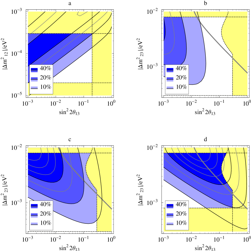
Figure 1: Contour lines for $|a^{\text{CP}}_{\nu_{\mu}\nu_{e}}/\sin\delta|$ in the $\sin^{2}2\theta_{13}$–$|\Delta m^{2}_{12}|$ plane for $|\Delta m^{2}_{23}|=2\cdot~{}10^{-3}\,\mathrm{eV}^{2}$ (a) and in the $\sin^{2}2\theta_{13}$–$|\Delta m^{2}_{23}|$ plane for $|\Delta m^{2}_{12}|=0.5\cdot 10^{-4}\,\mathrm{eV}^{2},2\cdot 10^{-4}\,\mathrm{eV}^{2},8\cdot~{}10^{-4}\,\mathrm{eV}^{2}$ (b,c,d) for $\sin^{2}2\theta_{12}=\sin^{2}2\theta_{23}=1$ and $\left\langle L/E\right\rangle\simeq 100\text{{m}}/\,\mathrm{MeV}$ (see text). The horizontal shadowed regions limit the range of $|\Delta m^{2}|$ according to eqs. (18) (and $|\Delta m^{2}_{23}|>|\Delta m^{2}_{12}|$ in (d)) whereas the shadowed regions on the right correspond to the combined Chooz and atmospheric neutrino limits. The thick solid line represents the MINOS sensitivity.

The general structure of figs. 1 can be easily understood with the help of the approximations yielding eq. (24). Fig. 1a shows that for maximal CP-violation ($|\sin\delta|=1$) the asymmetry can easily reach rather large values. Of course larger values of $|\Delta m^{2}_{12}|$ are preferred. As long as $\sin^{2}2\theta_{13}$ is not too small (otherwise the $\sin^{2}\Delta_{23}$ terms in eq. (2.2b) become as small as the $\sin^{2}\Delta_{12}$ ones and eqs. (3.1) is no longer valid) also smaller values of $\sin^{2}2\theta_{13}$ are preferred, as expected. Figs. 1b,c,d show the dependence on $|\Delta m^{2}_{23}|$ in greater detail.

As long as the approximations leading to eq. (24) hold, $|a^{\text{CP}}_{\nu_{\mu}\nu_{e}}/\sin\delta|\propto(\sin^{2}2\theta_{13})^{-1/2}$ for fixed $|\Delta m^{2}_{12}|$ and the contours are vertical a part from the (small) effects of $\sin^{2}\Delta_{23}$ in $\left\langle\sin^{2}\Delta_{23}\sin\Delta_{12}\right\rangle/\left\langle\sin^{2}\Delta_{23}\right\rangle$. On the other hand, for lower values of $|\Delta m^{2}_{23}|$ the $\sin^{2}\Delta_{12}$ terms in the CP-conserving part of the probability are not negligible anymore (otherwise eq. (24) would give $|a^{\text{CP}}_{\nu_{\mu}\nu_{e}}|>1$ for $\sin^{2}2\theta_{13}$ low enough). The value of $|\Delta m^{2}_{23}|$ at which the $\sin^{2}\Delta_{12}$ terms fold the contour-lines is higher when the $\sin^{2}\Delta_{23}$ term in is smaller, namely when $\sin^{2}2\theta_{13}$ is smaller, on the left-side of the plot.

In fig. 1b a “CP-disfavouring” value of $|\Delta m^{2}_{12}|=0.5\cdot 10^{-4}$ has been chosen, while in fig. 1c the “CP-optimistic” value $|\Delta m^{2}_{12}|=2\cdot 10^{-4}$ has been used. In fig. 1d a value of $|\Delta m^{2}_{12}|$ possible only in some non-standard solar analysis (see below) and therefore lying in the shadowed region in fig. 1a has been considered: $|\Delta m^{2}_{12}|=8\cdot 10^{-4}$. We see from figs. 1b,c that in case of maximal CP-violation the effects in the allowed region covered by the MINOS sensitivity range from 2% to 10% ($|\Delta m^{2}_{12}|=0.5\cdot 10^{-4}\,\mathrm{eV}^{2}$) and from 10% to 40% ($|\Delta m^{2}_{12}|=2\cdot 10^{-4}\,\mathrm{eV}^{2}$), according to the value of $|\Delta m^{2}_{23}|$ and the amplitude of the $\nu_{\mu}\rightarrow\nu_{e}$ oscillation.

Even in the framework of a standard analysis of solar data, these effects can therefore be large enough to spoil the analysis of a possible signal measured by a long-baseline experiment, if this analysis does not take into account CP-violation. In figs 1 this can be seen explicitely from the shown sensitivity goals of MINOS. Regarding the possibility of measuring such an asymmetry, it should be noticed that the asymmetry is larger when the amplitude is smaller, so that an enhancement of the CP-violation effect is accompanied by a suppression of the statistics. Thus there is no advantage from a statistical point of view. Large asymmetries should make it however easier to distinguish intrinsic from experimental asymmetries.

In some versions of solar neutrino data analysis $|\Delta m^{2}_{12}|$ can lie in the lower part of the atmospheric range. This can happen, for example, if one assumes an unknown large systematic error in the Chlorine experiment [6]. This is interesting, since the exclusion of the Chlorine data from the analysis makes the remaining solar data also consistent with an energy independent reduction of the solar flux as it happens to be above the MSW range and for almost maximal oscillation amplitude. As a consequence, for $\sin^{2}2\theta_{13}\lesssim 0.25$, as given by the Super-Kamiokande atmospheric analysis, the large angle solution becomes a vertical strip in the $|\Delta m^{2}_{12}|$-$\sin^{2}2\theta_{12}$ plane close to the $\sin^{2}2\theta_{12}=1$ axis and extending to the Chooz limit $|\Delta m^{2}_{12}|<10^{-3}\,\mathrm{eV}^{2}$. This explains why we considered in fig. 1d the possibility $|\Delta m^{2}_{12}|=8\cdot 10^{-4}\,\mathrm{eV}^{2}$, where the asymmetry is always large for maximal phases.

It is interesting to observe that the CP-violating part in the $\nu_{\mu}\rightarrow\nu_{e}$ amplitudes at long-baseline experiments can provide information on parameters typically accessible to solar neutrino experiments (at least in the present 3-neutrino scenario), while the CP-conserving part of the amplitudes are almost insensitive to the same parameters. The detection of a CP-violation effect would for example select the large angle MSW solution out of the three possible solutions of the solar neutrino problem. The values of $|a^{\text{CP}}_{\nu_{\mu}\nu_{e}}|$ and $\sin^{2}2\theta_{13}$, from the CP-conserving part, would select a range for $|\Delta m^{2}_{12}|$. This can be understood with the help of fig. 1a. The measurement of $\sin^{2}2\theta_{13}$ would select a vertical line in that plot. On the other hand, since that figure is “maximal”, namely plotted for $|\sin\delta|=1$, values of $|a^{\text{CP}}_{\nu_{\mu}\nu_{e}}|$ in this figure lower than the measured one would be ruled out, allowing thus only a limited range for $|\Delta m^{2}_{12}|$. Since lower values of $|\Delta m^{2}_{12}|$ would give a small CP-violation effect, such a measurement would select the upper part of the $|\Delta m^{2}_{12}|$ range provided by the solar analysis and larger asymmetries would correspond to stronger lower limits on $|\Delta m^{2}_{12}|$.

The parameters of our typical long baseline experiment are not too far away from the MSW resonance region. We must therefore include matter effects in our discussion as outlined in subsection 2.3 and we will now demonstrate that the corrections to the results obtained so far are moderate. Matter effects lead as usual to an inherent sensitivity of the charged current interactions of neutrinos to the electron flavour and diagonalization of the Hamiltonian leads to new mass eigenstates and shifted masses for the propagation in matter. The transition from vacuum to matter can altogether be phrased as two parameter mappings

$$(\theta_{12},\theta_{13},\theta_{23},\delta,\Delta m^{2}_{12},\Delta m^{2}_{23})\rightarrow(\theta_{12}^{\prime},\theta_{13}^{\prime},\theta_{23}^{\prime},\delta^{\prime},(\Delta m^{2}_{12})^{\prime},(\Delta m^{2}_{23})^{\prime})~{},$$ (25)

one for neutrinos and one for antineutrinos. In order to determine the corrections due to matter effects we studied for $f=\bar{f}$ numerically the asymmetry $a^{\mathrm{CP}}_{\mu e}$ for the following cases: a) $a^{\mathrm{CP}}_{\mu e}\equiv a^{\mathrm{tot}}_{\mu e}$ in vacuum for maximal CP-phase, b) $a^{\mathrm{tot}}_{\mu e}$ in matter with maximal phase, c) $a^{\mathrm{exp}}_{\mu e}$ in matter and d) $a^{\mathrm{CP}}_{\mu e}$ in matter with maximal phase.

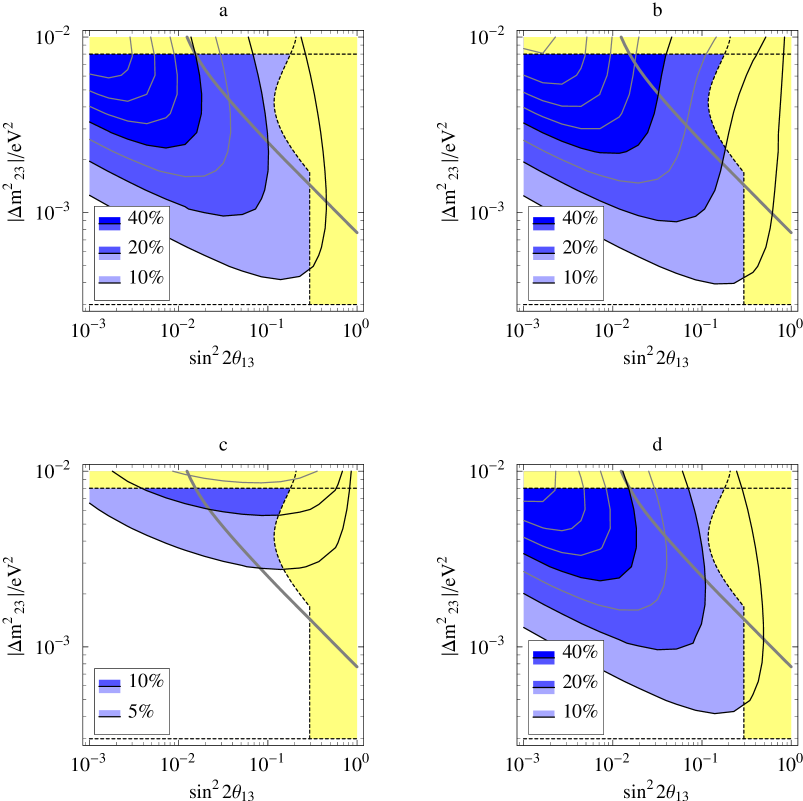
Figure 2: CP-asymmetries for the four cases discussed in the text in analogy to fig. 1: (a) $a^{\mathrm{CP}}_{\mu e}\equiv a^{\mathrm{tot}}_{\mu e}$ in vacuum for maximal CP-phase, (b) $a^{\mathrm{tot}}_{\mu e}$ in matter with maximal phase, (c) $a^{\mathrm{exp}}_{\mu e}$ in matter and (d) $a^{\mathrm{CP}}_{\mu e}$ in matter with maximal phase.

These asymmetries are plotted in figs. 2a–d for the $\nu_{\mu}\rightarrow\nu_{e}$ channel, where we use the scenario previously assumed for fig. 1c, namely a LBL experiment with $\left\langle L/E\right\rangle\simeq 100\mathrm{m}/\,\mathrm{MeV}$, $\delta m^{2}_{12}=2\cdot 10^{-4}\,\mathrm{eV}^{2}$ and $\sin^{2}2\theta_{12}=\sin^{2}2\theta_{23}=1$. Figure 2b shows the CP–asymmetry measured in the experiment, plot (c) the matter induced asymmetry and (d) the experimental asymmetry with the matter induced asymmetry subtracted. For a few parameter points these asymmetries were already calculated in [2] and our figures agree perfectly in those points. Note that matter effects depend both on the sign of $\Delta m^{2}$ and the sign of the CP-phase $\delta$. In fig. 2 we used a positive $\delta$ and a positive $\Delta m^{2}$, in which case matter and intrinsic effects go into the same direction.

Altogether we can see that matter effects require a generalization of the asymmetry in order to isolate genuine CP–violating effects from matter induced effects. Figures 2 show that the corrections are altogether moderate. Ideally one would like to study case d) which is due to intrinsic CP–violating effects, but would require to determine somehow $a^{\mathrm{exp}}_{\mu e}$ in matter. With good knowledge of the masses and mixing angles this may for example be possible by calculating this matter-induced asymmetry theoretically. To do so one has to use fig. 2b and subtract (with the correct sign) the theoretically calculated fig. 2c, which leads to larger systematic uncertainties. For fig. 2b the region with large CP-effects shifts to larger $\sin^{2}2\theta_{13}$ and smaller $\Delta m^{2}_{23}$ and the maximal CP-asymmetry expected in the sensitivity range of MINOS increases from 40% to 50%. This shows that the seperation is in principle possible, but it is clearly a difficult task which requires sufficient experimental information. Another promising method to seperate the matter-induced and intrinsic CP-asymmetries by using envelope patterns of the oscillation is discussed by Arafune, Koike and Sato [1].

3.2 Long-baseline $\nu_{\mu}\rightarrow\nu_{\tau}$

In the $\nu_{\mu}\rightarrow\nu_{\tau}$ channel the CP-violating probability is the same as in the $\nu_{\mu}\rightarrow\nu_{e}$ channel (a part from the sign) whereas the CP-conserving probability is not suppressed by $\sin^{2}2\theta_{13}$ anymore and is therefore larger. Therefore the asymmetry is smaller in this channel. On one hand the enhancement of the CP-conserving probability gives better statistics and hence in principle the possibility to appreciate a smaller asymmetry. This enhancement would on the other hand also enhance the “experimental” contribution $a^{\text{exp}}$ to the asymmetry, making it very hard to identify the CP-violating contribution $a^{\text{CP}}$. The $\nu_{\mu}\rightarrow\nu_{\tau}$ channel is therefore essentially unsuitable for the detection of CP-violating effects, and one can neglected them in the analysis of a possible signal. This statement is confirmed by fig. 3, where the contour lines for $|a^{\text{CP}}_{\nu_{\mu}\nu_{\tau}}/\sin\delta|$ are plotted in the $|\Delta m^{2}_{12}|$–$\sin^{2}2\theta_{13}$ plane for $|\Delta m^{2}_{23}|=2\cdot 10^{-3}\,\mathrm{eV}^{2}$ (a) and in the $|\Delta m^{2}_{23}|$–$\sin^{2}2\theta_{13}$ plane for the optimistic case $|\Delta m^{2}_{12}|=2\cdot 10^{-4}\,\mathrm{eV}^{2}$ (b). The figures show that the asymmetries are always smaller than 5%. Matter effects may then (via its asymmetric influnece on the mass eigenvalues) even dominate the asymmetry. Therefore we do not consider the $\mu$–$\tau$ channel any further.

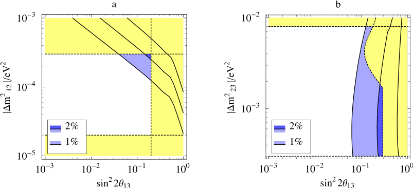
Figure 3: Contour lines for $|a^{\text{CP}}_{\nu_{\mu}\nu_{\tau}}/\sin\delta|$ in the $|\Delta m^{2}_{12}|$–$\sin^{2}2\theta_{13}$ plane for $|\Delta m^{2}_{23}|=2\cdot~{}10^{-3}\,\mathrm{eV}^{2}$ (a) and in the $|\Delta m^{2}_{23}|$–$\sin^{2}2\theta_{13}$ plane for $|\Delta m^{2}_{12}|=2\cdot 10^{-4}\,\mathrm{eV}^{2}$ (b) for $\sin^{2}2\theta_{12}=\sin^{2}2\theta_{23}=1$ and $\left\langle L/E\right\rangle\simeq 290\text{{m}}/\,\mathrm{MeV}$ (see text). The horizontal shadowed regions limit the range of $|\Delta m^{2}|$ according to eqs. (18) (and $|\Delta m^{2}_{23}|>|\Delta m^{2}_{12}|$ in (d)) whereas the shadowed regions on the right correspond to the combined Chooz and atmospheric neutrino limit.

4 Scenarios with four neutrinos

In order to accommodate the LSND signal in addition to the solar and atmospheric results we will study in this section four neutrinos scenarios. We expect that matter effects in long baseline experiments are moderate corrections like in the case of three neutrinos. The discussion of matter effects will therefore be covered elsewhere. Let us first consider the possible mass ordering schemes resulting from the hierarchical values of the squared mass differences $\Delta m^{2}_{\text{SUN}}\ll\Delta m^{2}_{\text{ATM}}\ll\Delta m^{2}_{\text{LSND}}$. As in the case of three neutrinos we associate the smallest squared mass difference with the first two mass eigenstates, i.e. $|\Delta m^{2}_{12}|=\Delta m^{2}_{\text{SUN}}$. Then there are only two possibilities for the ordering of the other mass differences relative to these first two states:

• The intermediate squared mass difference occurs between the 3rd and 4th eigenstates, i.e. $|\Delta m^{2}_{34}|=\Delta m^{2}_{\text{ATM}}$ and the larger LSND value defines the splitting between the 1st/2nd and 3rd/4th mass eigenstate. Altogether this implies $|\Delta m^{2}_{12}|\equiv\Delta m^{2}_{\text{SUN}}\ll|\Delta m^{2}_{34}|\equiv\Delta m^{2}_{\text{ATM}}\ll|\Delta m^{2}_{14}|\simeq|\Delta m^{2}_{24}|\simeq|\Delta m^{2}_{13}|\simeq|\Delta m^{2}_{23}|\equiv\Delta m^{2}_{\text{LSND}}$

• The intermediate squared mass difference occurs between one of the 1st and 2nd eigenstate and one eigenstate out of the 3rd and 4th. Conventionally they are the 2st and 3rd mass eigenstate, i.e. $|\Delta m^{2}_{23}|=\Delta m^{2}_{\text{ATM}}$ and the larger LSND value defines the splitting between the 4th mass eigenstate and the others, i.e. $|\Delta m^{2}_{34}|=\Delta m^{2}_{\text{LSND}}$. We have thus in this case $|\Delta m^{2}_{12}|\equiv\Delta m^{2}_{\text{SUN}}\ll|\Delta m^{2}_{13}|\simeq|\Delta m^{2}_{23}|\equiv\Delta m^{2}_{\text{ATM}}\ll|\Delta m^{2}_{14}|\simeq|\Delta m^{2}_{24}|\simeq|\Delta m^{2}_{34}|\equiv\Delta m^{2}_{\text{LSND}}$

Note that only $\Delta m^{2}$ enters in neutrino oscillation experiments and that this leaves some freedom in the ordering and absolute values of masses. Scheme B turns out to be in disagreement with experimental data [16]. We will therefore only consider scheme A in the following. This can be understood in a simplified picture where only two neutrino mass eigenstates (i.e. their $\Delta m^{2}$) participate in each oscillation experiment together with the information about the involved flavour transitions of each experiment. If one starts in scenario B with $\Delta m^{2}_{\text{SUN}}$ as the smallest quadratic mass splitting which involves $\nu_{e}$ and assumes that $\Delta m^{2}_{\text{ATM}}$ (which fixes $\nu_{\mu}$) comes next, then the third and largest $\Delta m^{2}_{\text{LSND}}$ could not be any longer an oscillation between $\nu_{\mu}$ and $\nu_{e}$, which is a contradiction with the LSND experiment.

Scenarios with four neutrinos involve in general a larger number of parameters in the mixing matrix with considerably more complexity in the parameter restrictions. The observed mass hierarchies allow however in experiments sensitive to $\Delta m^{2}\gtrsim 10^{-3}\,\mathrm{eV}^{2}$ the approximation $|\Delta m^{2}_{12}|\simeq 0$, unless $|\Delta m^{2}_{12}|$ is at the upper border or beyond its standard range, which will not be considered here. This approximation simplifies the general task considerably and reduces the number of involved parameters. Unlike the three neutrino case, in which $|\Delta m^{2}_{12}|$ could quite safely be neglected in the CP-conserving part of the probabilities while it was crucial in the CP-violating ones, $|\Delta m^{2}_{12}|$ can be safely neglected here completely. The oscillation probabilities are in the limit $|\Delta m^{2}_{12}|=0$ given by

$$\begin{split}\begin{picture}(22.0,10.0)\put(0.0,0.0){$P_{CP}$} \end{picture}(\nu_{e_{i}}\rightarrow\nu_{e_{j}})&=\delta_{ij}(1-4|U_{i4}|^{2}\sin^{2}\Delta_{24}-4|U_{i3}|^{2}\sin^{2}\Delta_{23})\hfill\\ &-4\operatorname{Re}J^{e_{j}e_{i}}_{34}\sin^{2}\Delta_{34}+4(\operatorname{Re}J^{e_{j}e_{i}}_{34}+\operatorname{Re}J^{e_{j}e_{i}}_{44})\sin^{2}\Delta_{24}\hfill\\ &+4(\operatorname{Re}J^{e_{j}e_{i}}_{33}+\operatorname{Re}J^{e_{j}e_{i}}_{34})\sin^{2}\Delta_{23}~{},\end{split}$$ (26a)

$$\begin{picture}(22.0,10.0)\put(8.0,-2.0){\line(2,1){12.0}} \put(0.0,0.0){$P_{CP}$} \end{picture}(\nu_{e_{i}}\rightarrow\nu_{e_{j}}) =8\operatorname{Im}J^{e_{j}e_{i}}_{34}(\sin^{2}\Delta_{23}\sin\Delta_{34}\cos\Delta_{34}+\sin^{2}\Delta_{34}\sin\Delta_{23}\cos\Delta_{23})~{},$$ (26b)

where the second and third line of (4a) are of special interest for our purposes.

Eq. (4b) shows that it is possible to generate the CP-violating part of the probabilities from $|\Delta m^{2}_{23}|$ and $|\Delta m^{2}_{34}|$. CP-violation in long-baseline experiments is therefore no longer suppressed by the small $\Delta m^{2}_{\text{SUN}}$ as in the three neutrino case and we will see that it can therefore be large. With four neutrinos one can also wonder, whether CP-violation can be important in short-baseline experiments able to measure small transition probabilities. We will see that, although the effects are not large, a modest improvement of $\left\langle L/E\right\rangle$ would be enough to see sizeable effects in the $\nu_{\mu}\rightarrow\nu_{\tau}$ channel, if the CP-violation phase is large. This is because the relative importance of CP-violation becomes larger for smaller effects, unlike what happens in the $\nu_{\mu}\rightarrow\nu_{e}$ case, where the relative importance of CP-violation is always small.

Concerning the possibility of CP-violation effects in atmospheric neutrino experiments, we notice that in the four neutrino case they are even more unlikely then in the three neutrino one. One may wonder why the four neutrino case does not contain the three neutrino scenario as a specific limit. This is however the case since there is one additional large frequency and also further constraints from experiments sensitive to that frequency. Especially important is here the constraint on $\nu_{e}\rightarrow\nu_{e}$ from the Bugey experiment which guarantees in this scenario that $\nu_{\mu}\leftrightarrow\nu_{e}$ oscillations (and therefore CP-violation, which appears only there) do not play a role in atmospheric neutrino oscillations. As a consequence CP-violation is negligible in atmospheric neutrino oscillations and we will therefore consider in the following only long- and short-baseline $\nu_{\mu}\rightarrow\nu_{e}$ and $\nu_{\mu}\rightarrow\nu_{\tau}$ experiments.

From eqs. (4) we can see that the oscillation probabilities between two different flavour eigenstates $\nu_{e_{i}}$ and $\nu_{e_{j}}$ depend only on the $2\times 2$ sub-sector of the mixing matrix involving the $i$th and $j$th flavour eigenstates and the 3rd and 4th mass eigenstates. That sub-matrix is described by 8 real parameters among which 3 are unphysical phases that can be rotated away, one is a physical phase and 4 are mixing parameters. We choose the 5 physical parameters as follows: Let $\nu^{\prime}_{e_{i}}=U_{i3}\nu_{3}+U_{i4}\nu_{4}$, $\nu^{\prime}_{e_{j}}=U_{j3}\nu_{3}+U_{j4}\nu_{4}$ be the projections of the flavour eigenstates $\nu_{e_{i}}$ and $\nu_{e_{j}}$ on the 3–4 mass eigenspace. Then we define analogous to ref. [17] the quantities $c_{i}$ and $c_{j}$ as the squared lengths of these projections, i.e. $c_{i}=|U_{i3}|^{2}+|U_{i4}|^{2}$, $c_{j}=|U_{j3}|^{2}+|U_{j4}|^{2}$. Furthermore $\theta_{i}\in[0,\pi/2]$ is the orientation of $\nu^{\prime}_{e_{i}}$ defined via $(|U_{i3}|,|U_{i4}|)=\sqrt{c_{i}}(\cos\theta_{i},\cos\theta_{j})$ and $\phi_{ij}\in[0,\pi/2]$ is the relative orientation of $\nu^{\prime}_{e_{i}}$ and $\nu^{\prime}_{e_{j}}$, $\cos\phi_{ij}=|U^{*}_{i3}U_{j3}+U^{*}_{i4}U_{j4}|/\sqrt{c_{i}c_{j}}$. Finally we define the relevant CP-violating phase as $\delta_{ij}=\mathrm{arg}(U^{*}_{i3}U_{j3}U^{*}_{j4}U_{i4})=\mathrm{arg}(J^{e_{j}e_{i}}_{34})$. The amplitudes of the oscillating terms in eqs. (4) can be expressed by these parameters to be

$$4\operatorname{Re}J^{e_{j}e_{i}}_{34}=c_{i}c_{j}\sin 2\theta_{i}(\cos 2\phi_{ij}\sin 2\theta_{i}+\sin 2\phi_{ij}\cos 2\theta_{i}\cos\delta_{ij})~{},$$ (27a)

$$4(\operatorname{Re}J^{e_{j}e_{i}}_{34}+\operatorname{Re}J^{e_{j}e_{i}}_{44})=4c_{i}c_{j}\sin\theta_{i}\cos\phi_{ij}(\cos\phi_{ij}\sin\theta_{i}+\sin\phi_{ij}\cos\theta_{i}\cos\delta_{ij})~{},$$ (27b)

$$4(\operatorname{Re}J^{e_{j}e_{i}}_{33}+\operatorname{Re}J^{e_{j}e_{i}}_{34})=4c_{i}c_{j}\cos\theta_{i}\cos\phi_{ij}(\cos\phi_{ij}\cos\theta_{i}-\sin\phi_{ij}\sin\theta_{i}\cos\delta_{ij})~{},$$ (27c)

$$4\operatorname{Im}J^{e_{j}e_{i}}_{34}=c_{i}c_{j}\sin 2\theta_{i}\sin 2\phi_{ij}\sin\delta_{ij}~{}.$$ (27d)

The introduced parameters $c_{i}$, $c_{j}$, $\theta_{i}$, $\phi_{ij}$, $\delta_{ij}$ can however not be chosen arbitrary since the $ij$/34 sub-matrix is part of a unitary matrix. The parameters must fulfill the following unitary constraints:

$$0\leq c_{i}\leq 1~{};\qquad 0\leq c_{j}\leq 1~{},$$ (28a)

$$c_{i}c_{j}\cos^{2}\phi_{ij}\leq(1-c_{i})(1-c_{j})~{}.$$ (28b)

These conditions can be easily understood noticing that the minor can be embedded in an unitary matrix if and only if the two $\mathbb{C}^{2}$ vectors $(U_{i3},U_{i4})$ and $(U_{j3},U_{j4})$ can be completed to a pair of orthonormal $\mathbb{C}^{4}$ vectors. Eq. (4a) corresponds then to the normalization condition and eq. (4a) to the orthogonality condition of the two $\mathbb{C}^{4}$ vectors.

The parameters $c_{i}$, $c_{j}$, $\theta_{i}$, $\phi_{ij}$, $\delta_{ij}$ are not only constrained by unitarity, but also by the results of the $\nu_{e}\rightarrow\nu_{e}$ and $\nu_{\mu}\rightarrow\nu_{\mu}$ disappearance, atmospheric neutrinos and LSND experiments. In order to make these constraints explicit, let us write the formulae for the relevant processes in the approximation where $|\Delta m^{2}_{34}|\ll|\Delta m^{2}_{23}|\simeq|\Delta m^{2}_{24}|$:

$$P(\nu_{e}\rightarrow\nu_{e}) \simeq 1-4c_{e}(1-c_{e})\sin^{2}\Delta_{23}-c_{e}^{2}\sin^{2}2\theta_{e}\sin^{2}\Delta_{34}~{},$$ (29a)

$$P(\nu_{\mu}\rightarrow\nu_{\mu}) \simeq 1-4c_{\mu}(1-c_{\mu})\sin^{2}\Delta_{23}-c_{\mu}^{2}\sin^{2}2\theta_{\mu}\sin^{2}\Delta_{34}~{},$$ (29b)

$$\begin{split}P(\nu_{\mu}\rightarrow\nu_{e})&\simeq 4c_{e}c_{\mu}\cos^{2}\phi_{\mu e}\sin^{2}\Delta_{23}+2c_{e}c_{\mu}\sin 2\theta_{\mu}\sin 2\phi_{\mu e}\sin\delta_{\mu e}\sin^{2}\Delta_{23}\sin\Delta_{34}\\ &\quad-c_{e}c_{\mu}\sin 2\theta_{\mu}(\cos 2\phi_{\mu e}\sin 2\theta_{\mu}+\sin 2\phi_{\mu e}\cos 2\theta_{\mu}\cos\delta_{\mu e})\sin^{2}\Delta_{34}~{}.\end{split}$$ (29c)

First we notice that only the $\sin^{2}\Delta_{23}$ term is relevant in eq. (4c) as far as the LSND experiment is concerned. The LSND oscillation probability can thus approximately be written as $P=A\cdot\sin^{2}\Delta_{23}$, where $A=4c_{e}c_{\mu}\cos^{2}\phi_{\mu e}$. The LSND results can thus be plotted conveniently in the $A$–$|\Delta m^{2}_{23}|$ plane. Moreover, the $\nu_{e}\rightarrow\nu_{e}$ and $\nu_{\mu}\rightarrow\nu_{\mu}$ disappearance experiments set upper limits both on the amplitudes of $\sin^{2}\Delta_{23}$ and $\sin^{2}\Delta_{34}$ on the r.h.s of eqs. (4a,b). We are interested in particular in the limits on $4c_{e}(1-c_{e})$ and $4c_{\mu}(1-c_{\mu})$, which correspond to two possible ranges for $c_{e}$ and $c_{\mu}$, each close to zero or one. For $c_{e}$, however, only the range around zero is allowed since the other close to one would suppress solar neutrino oscillations in an unacceptable way. Therefore we have a limit on $c_{e}$ in the form $0\leq c_{e}\leq a^{0}_{e}$  [16]. Concerning the range of $c_{\mu}$, the $\sin^{2}\Delta_{23}$ term in eq. (4b) is approximately constant in atmospheric neutrino experiments besides being constrained by disappearance experiments so that $c_{\mu}^{2}\sin^{2}2\theta_{\mu}$ must account for the zenith angle dependence of the measured $\nu_{\mu}$ flux. This selects out of the two possible ranges for $c_{\mu}$ the interval close to one, that can be written as $1-a^{0}_{\mu}\leq c_{\mu}\leq 1$. The other interval around zero would furthermore give a too small amplitude for the $\sin^{2}\Delta_{23}$ term in eq. (4c) accounting for the LSND signal, since it would give $A\leq 4a^{0}_{e}a^{0}_{\mu}$, which would exclude the LSND result (see fig. 4) [16]. Finally, since as said $c^{2}_{\mu}\sin^{2}2\theta_{\mu}\simeq\sin^{2}2\theta_{\mu}$ controls the zenith angle dependence of the atmospheric $\nu_{\mu}$ flux, we also have $\sin^{2}2\theta_{\mu}\simeq 1$. The constraint given by the LSND experiment on the parameters $c_{e}$, $c_{\mu}$, $\cos^{2}\phi_{\mu e}$, namely $4c_{e}c_{\mu}\cos^{2}\phi_{\mu e}=A$, has not been used in previous analysis. As we will see, it will play an important role in the following. The solar result does not give any further constraints for this discussion since we are in the limit where $\Delta m^{2}_{12}=0$.

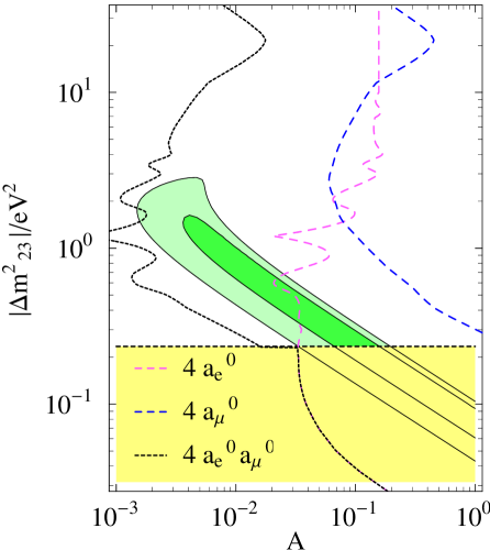
Figure 4: Constraints on the amplitude $A=4c_{e}c_{\mu}\cos^{2}\phi_{\mu e}$ of the LSND transition probability. The shown allowed regions in the LSND parameter space correspond to 90% and 99% C.L. The upper part of the plot is not shown because it is excluded by BNL E734. The dashed lines represent $4a^{0}_{e}$ (lighter) and $4a^{0}_{\mu}$ (darker), whereas the dotted line represents $4a^{0}_{e}a^{0}_{\mu}$. The shadowed region is excluded by the condition (31).

In the following subsection we will use eqs. (4,4) and the parameter constraints discussed above to study CP-violation in long- and short-baseline experiments.

4.1 Long- and short-baseline $\nu_{\mu}\rightarrow\nu_{e}$

Let us first identify the allowed parameter range. The viable scheme A) of squared mass differences implies of course $|\Delta m^{2}_{34}|=\Delta m^{2}_{\text{ATM}}=(0.3\mbox{--}9)\cdot 10^{-3}\,\mathrm{eV}^{2}$ and $|\Delta m^{2}_{23}|$ is of course the LSND range, $|\Delta m^{2}_{23}|=\Delta m^{2}_{\text{LSND}}=(0.04\mbox{--}2.8)\,\mathrm{eV}^{2}$. Furthermore the following constraints

$$0\leq c_{e}\leq a^{0}_{e}\quad 1-a^{0}_{\mu}\leq c_{\mu}\leq 1 \nu_{e}\rightarrow\nu_{e} \nu_{\mu}\rightarrow\nu_{\mu}$$ from , experiments (30a)

$$c_{e}c_{\mu}\cos^{2}\phi_{\mu e}\leq(1-c_{e})(1-c_{\mu})$$ from unitarity (30b)

$$4c_{e}c_{\mu}\cos^{2}\phi_{\mu e}=A$$ from LSND (30c)

have to be simultaneously satisfied. It is shown in Appendix B that eqs. (4.1) can be fulfilled if and only if

$$A\leq\min\left(4a^{0}_{\mu}(1-a^{0}_{\mu}),4a^{0}_{e}(1-a^{0}_{e})\right)\simeq\min\left(4a^{0}_{\mu},4a^{0}_{e}\right)~{}.$$ (31)

This gives a restriction on the $|\Delta m^{2}_{23}|$ range shown in fig. 4 (the shadowed region is excluded, the function $\min(4a^{0}_{\mu},4a^{0}_{e})$ can easily be recovered from the dashed lines).

From eqs. (4,4) it is easy to see that the CP-asymmetries $a^{\text{CP}}_{\nu_{\mu}\nu_{e}}$ do not depend explicitely on $c_{e}$, $c_{\mu}$. Eq. (4.1c) introduces however a dependence on $c_{e}$, $c_{\mu}$ since $\cos^{2}\phi_{\mu e}$ is a function of $c_{e}$, $c_{\mu}$. It is therefore important to know the allowed ranges of $c_{e}$ and $c_{\mu}$. Eq. (4.1a) alone does not guarantee that it is possible to fulfill eqs. (4.1b,c). It turns out that it is possible to find $c_{\mu}$ and $\phi_{\mu e}$ by solving (4.1b,c) if and only if

$$\frac{A}{4}\simeq\frac{1-\sqrt{1-A}}{2}\leq c_{e}\leq\min\left(a^{0}_{e},1-\frac{A}{4a^{0}_{\mu}}\right)~{}.$$ (32)

This is a non-wide range when eq. (31) is fulfilled. For a given $c_{e}$ in the range of eq. (32) the possible values of $c_{\mu}$ are those fulfilling simultaneously

$$\frac{A}{4c_{e}}\leq c_{\mu}\leq 1-\frac{A}{4(1-c_{e})}\qquad\text{and}\qquad c_{\mu}\geq 1-a^{0}_{\mu}~{}.$$ (33)

In this case $A/(4c_{e}c_{\mu})\leq 1$ and $\phi_{\mu e}$ is determined by

$$\cos^{2}\phi_{\mu e}=\frac{A}{4c_{e}c_{\mu}}~{},$$ (34)

where $c_{\mu}=1$ can be used as a good approximation.

Finally we have all the necessary ingredients to discuss CP-violation in terms of the quantity $|a^{\text{CP}}_{\nu_{\mu}\nu_{e}}/\sin\delta_{\mu e}|$ which depends mostly only on $|\Delta m^{2}_{34}|$, $|\Delta m^{2}_{23}|$, $c_{e}$, with the ranges given by eq. (18a), eq. (31) and eq. (32) respectively. The dependence on $\sin^{2}2\theta_{\mu}$ is in fact negligible since $\sin^{2}2\theta_{\mu}\simeq 1$ and we can therefore set $\sin^{2}2\theta_{\mu}=1$ without affecting our results too much. Analogously, we set $c_{\mu}=1$. The dependence of $|a^{\text{CP}}_{\nu_{\mu}\nu_{e}}/\sin\delta_{\mu e}|$ on $\delta_{\mu e}$ is also negligible in the limit $|\Delta m^{2}_{34}|\ll|\Delta m^{2}_{23}|$.

As a consequence of the Bugey limit, the amplitude of the $\nu_{\mu}\rightarrow\nu_{e}$ oscillation in a short-baseline experiment is necessarily small. One may wonder if such a small oscillation can be accompanied by relatively large CP-violation as it can happen in the three neutrino scenario. To see that this is not the case it is enough to study the qualitative features of $|a^{\text{CP}}_{\nu_{\mu}\nu_{e}}/\sin\delta_{\mu e}|$ analytically. With the approximations $\sin^{2}\Delta_{24}\simeq\sin^{2}\Delta_{23}$ and $\sin^{2}2\theta_{\mu}=1$ one gets

$$\left|\frac{a^{\text{CP}}_{\nu_{\mu}\nu_{e}}}{\sin\delta_{\mu e}}\right|\simeq\left|\frac{4\sin\phi_{\mu e}\cos\phi_{\mu e}\left\langle\sin^{2}\Delta_{23}\sin\Delta_{34}\right\rangle}{4\cos^{2}\phi_{\mu e}\left\langle\sin^{2}\Delta_{23}\right\rangle-\cos 2\phi_{\mu e}\left\langle\sin^{2}\Delta_{34}\right\rangle}\right|$$ (35)

and in particular

$$\left|\frac{a^{\text{CP}}_{\nu_{\mu}\nu_{e}}}{\sin\delta_{\mu e}}\right|\simeq\left|\tan\phi_{\mu e}\frac{\left\langle\sin^{2}\Delta_{23}\sin\Delta_{34}\right\rangle}{\left\langle\sin^{2}\Delta_{23}\right\rangle}\right|$$ (36)

for short-baseline experiments. Even in the “CP-optimistic”case with $|\Delta m^{2}_{23}|=8\cdot 10^{-3}\,\mathrm{eV}^{2}$ eq. (36) is rather strongly suppressed by $\sin\Delta_{34}$ in a short-baseline experiment. Measurable effects could only show up if an enhancement by a large $\tan\phi_{\mu e}$ were possible, which would require via eq. (34) a rather small value of $A/4c_{e}$. The smallest value of $A$ allowed by the LSND plot and the maximal value of $c_{e}$ allowed by eq. (32) do however not allow values of $A/c_{e}$ much smaller than one. CP-violation is consequently expected to be negligible which is confirmed by fig. 5a, where the contour lines for $|a^{\text{CP}}_{\nu_{\mu}\nu_{e}}/\sin\delta|$ are plotted in the $c_{e}$–$|\Delta m^{2}_{23}|$ plane using the exact formulas eqs. (4,4) for the oscillation probability for an optimistic value of $|\Delta m^{2}_{34}|=8\cdot 10^{-3}\,\mathrm{eV}^{2}$. The assumed experimental setup is $L\simeq 0.5\,\text{km}$ and a broad distribution for $E$ around $1\,\mathrm{GeV}$ which looks like MiniBooNE. Fig. 5a shows that the asymmetry does not exceed 3%, even for maximal phase.

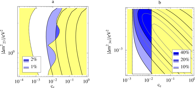
Figure 5: Contour lines for $|a^{\text{CP}}_{\nu_{\mu}\nu_{e}}/\sin\delta_{\mu e}|$ in a four neutrino scenario plotted in the $c_{e}$–$|\Delta m^{2}_{23}|$ parameter space of a short-baseline experiment for $|\Delta m^{2}_{34}|=8\cdot 10^{-3}\,\mathrm{eV}^{2}$ (a) and in the $c_{e}$–$|\Delta m^{2}_{34}|$ plane of a long-baseline experiment for $|\Delta m^{2}_{23}|=1\,\mathrm{eV}^{2}$ (b). Only the allowed $|\Delta m^{2}|$ ranges are shown. The shadowed regions are excluded by the constraints (32).

Long-baseline experiments are of course not $\sin\Delta_{34}$ suppressed and the $\sin^{2}\Delta_{23}$ dependence becomes negligible since it is washed out by averaging over the $L/E$ spectrum. Eq. (35) becomes thus

$$\left|\frac{a^{\text{CP}}_{\nu_{\mu}\nu_{e}}}{\sin\delta_{\mu e}}\right|\simeq\left|\frac{2\sin\phi_{\mu e}\cos\phi_{\mu e}\left\langle\sin\Delta_{34}\right\rangle}{2\cos^{2}\phi_{\mu e}-\cos 2\phi_{\mu e}\left\langle\sin^{2}\Delta_{34}\right\rangle}\right|~{}.$$ (37)

CP-violation in this case is not suppressed at all. This can be seen directly from fig. 5b, where contour lines for $|a^{\text{CP}}_{\nu_{\mu}\nu_{e}}/\sin\delta_{\mu e}|$ are plotted in the $c_{e}$–$|\Delta m^{2}_{34}|$ plane for $|\Delta m^{2}_{23}|=1\,\mathrm{eV}^{2}$ in a “MINOS-like” long-baseline experiment like described in the previous section. The unshadowed rectangular window in fig. 5b represents the values of $c_{e}$ which are allowed by the Bugey experiment and the unitarity constraint. The CP-asymmetry in the allowed region can reach 60% for a maximal CP-violating phase. This leads to the important question whether the allowed region could be reached by a long-baseline experiment despite the strong constraint from Bugey. The answer depends on the value of $|\Delta m^{2}_{23}|$ and $\delta_{\mu e}$ but in many cases is yes. A definitive answer would require a plot of the sensitivity of a long-baseline experiment (here we consider MINOS again) in the allowed region of the parameter space. The published sensitivity plots are however for the parameter space $\{A,\Delta m^{2}\}$ of a simple two neutrino oscillation in which the transition probability is given by $P=A\sin^{2}\Delta m^{2}L/(4E)$. The $\nu_{\mu}\rightarrow\nu_{e}$ transition probability cannot be reduced to that form in our case being rather

$$P(\nu_{\mu}\rightarrow\nu_{e})\simeq A/2+c_{e}(-\cos 2\phi_{\mu e}\left\langle\sin^{2}\Delta_{34}\right\rangle\pm\sin 2\phi_{\mu e}\sin\delta_{\mu e}\left\langle\sin\Delta_{34}\right\rangle)~{},$$ (38)

where the sign of the $\left\langle\sin\Delta_{34}\right\rangle$ term depends on the sign of $\sin 2\theta_{\mu}$ and can be reabsorbed in the definition of $\delta_{\mu e}$. $A$ is the LSND amplitude given in fig. 4 and eq. (4.1c) has been used. The sensitivity in the $c_{e}$–$|\Delta m^{2}_{34}|$ plane depends therefore on $\sin\delta_{\mu e}$, which controls the interference in eq. (38), and on $A$ (and in turn on $|\Delta m^{2}_{23}|$) mainly through the $A/2$ term. Clearly larger values of $A$ are preferred and it turns out that the sensitivity is larger for positive values of $\sin\delta$. For example the sensitivity obtained for $\sin\delta=1$ and $|\Delta m^{2}_{23}|=1\,\mathrm{eV}^{2}$ allows to reach most of parameter space. Values of $A$ which are in better agreement the KARMEN experiment give less sensitivity and the smallest possible value of $A$ allowed by LSND at 99% CL would give a transition probability too small to be measured. Nevertheless a long-baseline $\nu_{\mu}\rightarrow\nu_{e}$ experiment along the line discussed has in a four neutrino scenario a good chance to observe oscillation and this oscillation would most likely contain a sizable or even large CP-violating part.

4.2 Long- and short-baseline $\nu_{\mu}\rightarrow\nu_{\tau}$

Unlike what we have seen in the three neutrino case, here the $\nu_{\mu}\rightarrow\nu_{\tau}$ channel turns out to be very interesting. From the previous subsection it is immediately clear that the relevant parameters are now $|\Delta m^{2}_{23}|$, $|\Delta m^{2}_{34}|$, $\theta_{\mu}$, $c_{\mu}$, $c_{\tau}$, $\phi_{\mu\tau}$ and $\delta_{\mu\tau}$. The parameters $|\Delta m^{2}_{23}|$, $|\Delta m^{2}_{34}|$, $\theta_{\mu}$ and $c_{\mu}$ are constraint as before. The unitarity constraints eqs. (4) for the $\mu\tau$/34 sub-matrix give now additionally the conditions

$$0\leq c_{\tau}\leq 1~{},$$ (39a)

$$c_{\mu}c_{\tau}\cos^{2}\phi_{\mu\tau}\leq(1-c_{\mu})(1-c_{\tau})~{},$$ (39b)

while $c_{\mu}$ is already known to be in the range

$$\max(1-a^{0}_{\mu},\frac{A}{4a^{0}_{e}})\equiv c_{\mu}^{\text{min}}\leq c_{\mu}\leq\frac{1+\sqrt{1-A}}{2}~{}.$$ (40)

In addition to the transition probabilities already given in eqs. (4) there is now the $\nu_{\mu}\rightarrow\nu_{\tau}$ channel

$$P(\nu_{\mu}\rightarrow\nu_{\tau})\simeq 4c_{\mu}c_{\tau}\cos^{2}\phi_{\mu\tau}\sin^{2}\Delta_{23}+2c_{\mu}c_{\tau}\sin 2\theta_{\mu}\sin 2\phi_{\mu\tau}\sin\delta_{\mu\tau}\sin^{2}\Delta_{23}\sin\Delta_{34}\\ -c_{\mu}c_{\tau}\sin 2\theta_{\mu}(\cos 2\phi_{\mu\tau}\sin 2\theta_{\mu}+\sin 2\phi_{\mu\tau}\cos 2\theta_{\mu}\cos\delta_{\mu\tau})\sin^{2}\Delta_{34}~{}.$$ (41)

Let us consider first a short-baseline experiment. Among the oscillating terms only $\sin^{2}\Delta_{23}$ can develop and contribute to this transition probability. The r.h.s. of eq. (41) is therefore to a very good approximation given by the first term which is furthermore suppressed by the unitarity constraints on $c_{\mu}$ and $c_{\tau}$. This suppression turns out to be much less effective in the CP-violating part, whose relative importance grows therefore when the total probability gets smaller, very much like in the three neutrino $\nu_{\mu}\rightarrow\nu_{e}$ case. One obtains for the short-baseline case

$$\left|\frac{a^{\text{CP}}_{\nu_{\mu}\nu_{\tau}}}{\sin\delta_{\mu\tau}}\right|\simeq\left|\tan\phi_{\mu\tau}\frac{\left\langle\sin^{2}\Delta_{23}\sin\Delta_{34}\right\rangle}{\left\langle\sin^{2}\Delta_{23}\right\rangle}\right|~{},$$ (42)

and we can see that the $\sin\Delta_{34}$ suppression can be compensated by large values of $\tan\phi_{\mu\tau}$. In fig. 6a we show contour lines for $|a^{\text{CP}}_{\nu_{\mu}\nu_{\tau}}/\sin\delta_{\mu\tau}|$ in the $\cos^{2}\phi_{\mu\tau}$–$|\Delta m^{2}_{34}|$ plane for $|\Delta m^{2}_{23}|=1\,\mathrm{eV}^{2}$ for the short baseline experiment described in the previous subsection. The maximum possible sensitivity of such an experiment is within the non-shadowed region. The sensitivity in less favourable cases is also shown. The precise way how the sensitivity was here obtained and the meaning of the “less favourable cases” is explained in greater detail in the following long-baseline case.

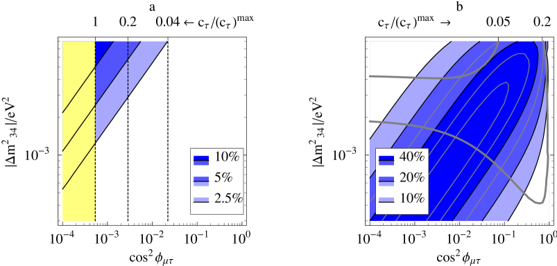
Figure 6: Contour lines for $|a^{\text{CP}}_{\nu_{\mu}\nu_{\tau}}/\sin\delta_{\mu\tau}|$ in the $\cos^{2}\phi_{\mu\tau}$–$|\Delta m^{2}_{34}|$ plane for $|\Delta m^{2}_{23}|=1\,\mathrm{eV}^{2}$ (a) for the short-baseline experiment and (b) for the long-baseline experiment discussed in the text. The accessible parameter space of such an experiment depends on $c_{\tau}$. The non-shadowed region shows the optimal case of $c_{\tau}=c_{\tau}^{max}$ which covers the whole plot in (b). The dashed lines show the sensitivity in less favourable cases with $c_{\tau}<c_{\tau}^{max}$ (see labels above figure and text). Everything to the right of the dashed lines in (a) can be explored by the discussed experiment whereas in (b) the whole area from the upper-left corner to the dashed lines lies within the sensitivity of the experiment.

Contrarily to what happened in the three neutrino $\nu_{\mu}\rightarrow\nu_{e}$ case, in which the necessary enhancement was obtained within the sensitivity of the experiment, the necessary enhancement is here outside the reach of an experiment like MiniBooNE. Note however that an enhancement by a factor $\sim 10$ in $\left\langle L/E\right\rangle\sim 0.5$ of the assumed short-baseline experiment would be enough to test CP-violation, which can be seen by multiplying the asymmetry in fig. 6a by $\left\langle L/E\right\rangle/0.5$. It is therefore not necessary to go a long-baseline one with $\left\langle L/E\right\rangle\sim 100$ to test CP-violation.

Finally we can also discuss in the four neutrino case CP-violation in a long-baseline experiment like that considered in the three neutrino case. The corresponding contour lines for $|a^{\text{CP}}_{\nu_{\mu}\nu_{\tau}}/\sin\delta_{\mu\tau}|$ are shown in fig. 6b as before in the $\cos^{2}\phi_{\mu\tau}$–$|\Delta m^{2}_{34}|$ plane for fixed $|\Delta m^{2}_{23}|=1\,\mathrm{eV}^{2}$. The precise value of $|\Delta m^{2}_{23}|$ is anyway irrelevant since $\sin^{2}\Delta_{23}$ is averaged to $1/2$ in this case. The asymmetry is in this case also completely independent of $c_{\mu}$, $c_{\tau}$ and the dependence on $\theta_{\mu}$ is negligible as before. What matters is again the region of parameter space accessible to the experiment, which depends on $c_{\tau}$ in the way given by eq. (41). The range of $c_{\tau}$, which is determined by eqs. (4.2) in terms of $\cos^{2}\phi_{\mu\tau}$, is therefore crucial and one finds

$$0\leq c_{\tau}\leq\frac{1-c_{\mu}^{\text{min}}}{1-c_{\mu}^{\text{min}}\sin^{2}\phi_{\mu\tau}}~{}.$$ (43)

The sensitivities of fig. 6b depend therefore on the chosen value of $c_{\tau}$ and become maximal for the largest possible value $c_{\tau}^{\text{max}}\equiv\frac{1-c_{\mu}^{\text{min}}}{1-c_{\mu}^{\text{min}}\sin^{2}\phi_{\mu\tau}}$. For this maximal value $c_{\tau}=c_{\tau}^{\text{max}}$ one finds that the experimental sensitivity covers the complete coordinate range of fig. 6b and only rather small values of $c_{\tau}$ make some of the relevant parts of the parameter space unaccessible. We show in fig. 6b the sensitivity corresponding to $c_{\tau}=0.2\,c_{\tau}^{\text{max}}$ and $c_{\tau}=0.05\,c_{\tau}^{\text{max}}$. The region to the right of the 20% (5%) sensitivity line are excluded if $c_{\tau}$ is less than 20% (5%) of its maximum value in that region. One can see that $c_{\tau}=0.2\,c_{\tau}^{\text{max}}$ still allows to reach the interesting region whereas $c_{\tau}=0.05\,c_{\tau}^{\text{max}}$ excludes it. Here, as in the $\nu_{\mu}\rightarrow\nu_{e}$ case, the sensitivity depends on the sign of $\sin 2\theta_{\mu}$ and on the CP-violating phases, that control the interference between the CP-violating and CP-conserving parts of the transition probabilities. The lines plotted correspond to $\sin 2\theta_{\mu}=1$, $\sin\delta_{\mu\tau}=1$, that give a better sensitivity. The results of this subsection show that $\nu_{\mu}\rightarrow\nu_{\tau}$ is a good place to look for CP-violation in four neutrino scenarios even with intermediate-baseline experiments. Moreover, if there are four neutrinos and if a signal is observed, CP-violation should be taken into account in an analysis.

5 Discussion and Conclusions

We studied in this paper CP-violation in neutrino oscillation and discussed the sensitivity for such effects of current and future experiments. As a measure of CP-violation, we considered asymmetries between CP-conjugated transition probabilities. These asymmetries are a measure of the relative strength of CP-violating effects. They are therefore very useful in studying how much CP-violation would affect the measurement of oscillation in one of the two CP-conjugated channels. The contribution from CP-violation has to be separated however from the experimental asymmetries between the two channels, which we assumed to be small or under control.

The fact that it is not possible to accommodate the claimed three independent oscillation signals in scenarios with three neutrinos led us to a twofold strategy. The first scenario was to leave out one evidence for oscillation and to analyze the case of three neutrinos. Since the LSND evidence is almost in contradiction with KARMEN it is considered most controversial and we omitted it therefore in the three neutrino case. The second case which was studied includes LSND in a four neutrino scenario. In both cases all further existing exclusion limits were taken into account. The two scenarios lead to quite different results with different sizes of CP-violating effects. In all cases we present results for maximal CP-phase, which can be easily rescaled to an arbitrary value.

For three neutrinos CP-violating effects are drastically suppressed by small angles or by extremely small $\Delta m^{2}$ in the case of the small mixing angle MSW-solution and for the vacuum solution. The large mixing angle MSW-solution allows however sizable CP-violating effects in long-baseline experiments, while there is no effect in short-baseline experiments. In the $\mu\rightarrow e$ channel we found in long-baseline experiments for maximal CP-phase $\delta$ effects up to 40%, while we found only small effects in the $\mu\rightarrow\tau$ channel. The observation of CP-violation would also allow to distinguish between the different solar solutions and can even further restrict the parameter space for $|\Delta m_{12}^{2}|$. Including matter effects in these long baseline experiments we found for the considered setup moderate corrections compared to the case without matter. Depending on the sign of the squared mass difference, the total intrinsic CP-asymmetry in $\mu\rightarrow e$ oscillation can be enhanced up to 50%. In $\mu\rightarrow\tau$ oscillation matter effects dominate the asymmetry since the intrinsic CP-violation is very small and therefore anyway uninteresting.

In order to include the LSND result we studied also the case of four neutrinos where many more parameters exist in principle. The solar $\Delta m^{2}$-value is in this case unimportant since CP-violating effects can be generated by the larger $\Delta m^{2}$ responsible for the atmospheric neutrino oscillations and for the LSND measurement. For experiments which are only sensitive to $\Delta m^{2}\geq 10^{-3}~{}eV^{2}$, we could make the approximation $\Delta m_{12}^{2}=0$ which reduces the number of relevant parameters drastically and allows a study of the available parameter space. The CP-violating effects are now in the case of four neutrinos potentially larger and we considered therefore also short-baseline experiments. Altogether we find in the four neutrino scenario for maximal CP-phase the following effects: In short-baseline $\mu\rightarrow e$ experiments less than 2 %, in short-baseline $\mu\rightarrow\tau$ up to 10 % and in long-baseline $\mu\rightarrow e$ as well as $\mu\rightarrow\tau$ experiments up to 60 %. The effects are not very big in the considered MiniBooNE-like short-baseline setup, but we want to point out, that a modest improvement of $\left\langle L/E\right\rangle\simeq 0.5$ by a factor 10 would be enough to test CP-violation in the $\nu_{\mu}\rightarrow\nu_{\tau}$ channel.

We did not consider cases with more than four neutrino mass eigenstates. It should however be clear from the current analysis that large CP-violating effects could easily be involved in that case in current and/or future neutrino oscillation experiments.

In summary we found that CP-violating effects can be surprisingly large in some future neutrino oscillation experiments and such effects should therefore be included in the analysis. Besides the obvious general interest for a determination of CP-violation connected to the theoretical questions on physics beyond the Standard Model and the potential role which CP-violation could play in lepto– and baryogenesis, there are further reasons why CP-violation should be taken into account. The main point is that the omission of CP-violation can spoil a two or three neutrino analysis that does not take it into account. Moreover, if an asymmetry between CP-conjugated transitions were measured and the presence of light sterile neutrinos would be excluded, it would discriminate between the different solar solutions and set lower bounds on the solar $\Delta m^{2}$.

Acknowledgments: We are grateful to E. Akhmedov, S. Bilenky and M.B. Gavela for useful comments and discussions. AR wishes to thank the Institutes T30d and T31 at the Physics Department of the Technical University of Munich for their warm hospitality.

Appendix A

A non-standard solar analysis allows in principle the possibility that $|\Delta m^{2}_{12}|$ falls in the atmospheric range, but still consistent with the Chooz constraint. For this case one may wonder whether

• $|\Delta m^{2}_{12}|$ could be responsible for both the solar evidences (with Chlorine excluded) and the atmospheric results with $|\Delta m^{2}_{23}|$ above the atmospheric range (to account for cosmological requirements on neutrino masses)

and whether

• $|\Delta m^{2}_{23}|$ could explain the LSND signal.

The answers to these two questions are that, independently of ii), i) is strongly disfavoured and that ii) is not possible. i) is disfavoured independently of the possibility of explaining LSND for two reasons. First of all the probability that $|\Delta m^{2}_{12}|$ is in the part of the atmospheric range which is not excluded by the Chooz constraint is small. This, together with the solar constraints which exclude large $|U_{e3}|^{2}$ gives $|U_{e3}|^{2}\lesssim 0.025$. The survival probability for solar neutrino state $\nu_{2}$ is therefore $P(\nu_{e}\rightarrow\nu_{e})=1-\sin^{2}2\theta_{12}\sin^{2}\Delta_{12}$ with $\sin^{2}2\theta_{12}\simeq 1$ which has to explain the solar data (with Chlorine excluded). This is on the other hand in this scenario also the survival probability for atmospheric $\nu_{e}$ appearing in eq. (2.4b). The atmospheric fit would in this case therefore be very bad, since the the zenith angle variation of $R_{e}$ in eqs. (2.4) would be larger than for $R_{\mu}$.

LSND cannot be explained in any case, even if the two points above are ignored. The LSND oscillation probability is for this scenario

$$P(\bar{\nu}_{\mu}\rightarrow\bar{\nu}_{e})=4|U_{e3}U_{\mu 3}|^{2}\sin^{2}\Delta_{23}~{}.$$ (44)

The mixing $|U_{e3}|^{2}$ is known to be small with the upper limit given by Bugey. The mixing $|U_{\mu 3}|^{2}$ is also small because $4|U_{\mu 1}U_{\mu 2}|^{2}\leq(1-|U_{\mu 3}|^{2})^{2}$ has to be maximal in order to explain the oscillation of $R_{\mu}$ in eq. (2.4a) and because of the experimental limit given by CDHS and CCFR. Combining these two limits into a single limit for $4|U_{e3}U_{\mu 3}|^{2}$ one finds that the probability in eq. (44) is too small to explain the LSND signal [17].

Appendix B

In this appendix we prove the statements concerning the range of $c_{e}$, $c_{\mu}$, $\phi_{\mu e}$ satisfying eqs. (4.1). First we prove that eq. (31) is sufficient for the existence of a solution to these equations. Therefore it is enough to check that $c_{e}=c^{\text{min}}$, $c_{\mu}=c^{\text{max}}$, $\phi_{\mu e}=0$ are a solution of eqs. (4.1). Then we prove that eq. (31) is also a necessary condition. From eqs. (4.1b,c) follows $4c_{e}c_{\mu}\geq A$ and $4(1-c_{e})(1-c_{\mu})\geq A$ and therefore $c_{e}\geq A/(4c_{\mu})$, $c_{\mu}\leq 1-A/(4(1-c_{e}))$. In particular we have $4c_{e}^{2}-4c_{e}+A\leq 0$ and $4c_{\mu}^{2}-4c_{\mu}+A\leq 0$ so that, together with the previous relations, we obtain

$$c_{e}\geq c^{\text{min}}=\frac{1-\sqrt{1-A}}{2}\simeq\frac{A}{4}~{};\qquad c_{\mu}\leq c^{\text{max}}=\frac{1+\sqrt{1-A}}{2}\simeq 1-\frac{A}{4}~{}.$$

But in order to satisfy eq. (4.1a) one must have $c^{\text{min}}\leq a^{0}_{e}$ and $c^{\text{max}}\geq 1-a^{0}_{\mu}$, namely

$$A\leq 4a^{0}_{e}(1-a^{0}_{e})\quad\text{and}\quad A\leq 4a^{0}_{\mu}(1-a^{0}_{\mu})~{}.$$

Let us now prove eq. (32). To begin, let us consider a given value of $c_{e}$. Eqs. (4.1b,c) give

$$\frac{A}{4c_{e}}\leq c_{\mu}\leq 1-\frac{A}{4(1-c_{e})}~{},$$ (45)

where a solution exists when eq. (31) holds. Since $1-a^{0}_{\mu}\leq c_{\mu}\leq 1$, $1-A/(4(1-c_{e}))$ must be equal to or larger than $1-a^{0}_{\mu}$ in order to obtain a finite range for $c_{\mu}$. One finds thus

$$c_{e}\leq 1-\frac{A}{4a^{0}_{\mu}}~{},$$

which, together with the previous bounds, gives eq. (32). To see that eq. (32) is not an empty interval we have to check that $c^{\text{min}}_{e}\leq 1-A/(4a^{0}_{\mu})$. This is a consequence of $A=(1-c^{\text{min}}_{e})(1-c^{\text{max}}_{\mu})$ and $c^{\text{max}}_{\mu}\geq 1-a^{0}_{\mu}$. The range of $c_{\mu}$ for a given value of $c_{e}$, eq. (33), then follows from what we saw.

References

-
[1]
V. Barger, Yuan-Ben Dai, K. Whisnant and Bing-Lin Young,
Neutrino Mixing, CP/T Violation and Textures in Four-Neutrino Models,
hep-ph/9901388;
K.R. Schubert, May We Expect CP- and T-Violating Effects in Neutrino Oscillations?, hep-ph/9902215;
J. Arafune, M. Koike and J. Sato, Phys. Rev. D56 (1997) 3093;
M. Tanimoto, Phys. Lett. B435 (1998) 373;
H. Minakata and H. Nunokawa, Phys. Rev. D57 (1998) 4403. - [2] A.De Rújula, M.B. Gavela and P. Hernández, Neutrino Oscillation Physics with a Neutrino Factory, hep-ph/9811390.
- [3] J.N. Bahcall, S. Basu and M.H. Pinsonneault, Phys. Lett. B433 (1998) 1.
- [4] J. N. Bahcall, P. I. Krastev and A. Y. Smirnov, Phys. Rev. D58 (1998) 096016.
- [5] Super-Kamiokande Collaboration, Phys. Rev. Lett. 82 (1999) 1810.
- [6] R. Barbieri, L. J. Hall, D. Smith, A. Strumia and N. Weiner, Journal of High Energy Physics, JHEP 9812 (1998) 017.
- [7] Super-Kamiokande Collaboration, T. Kajita, in Neutrino 98, Proceeding of the XVIII International Conference on Neutrino Physics and Astrophysics, Takayama, Japan, 4-9 June 1998, edited by Y.Suzuki and Y. Totsuka.
- [8] C. Athanassopoulos et al., LSND Coll., Phys. Rev. C58 (1998) 2489.
- [9] Chooz Collaboration, Phys. Lett. B420 (1998) 397.
- [10] CHORUS Collaboration, New Results on the Oscillation Search with the CHORUS Detector, hep-ex/9807024.
- [11] B. Achkare et al., Nucl. Phys. B434 (1995) 503.
- [12] F. Dydak et al., Phys. Lett. B134 (1984) 281.
- [13] I. E. Stockdale et al., Phys. Rev. Lett. 52 (1984) 1384.
- [14] V. Barger, T. J. Weiler and K. Whisnant, Phys. Lett. B440 (1998) 1.
- [15] Super-Kamiokande Collaboration, Phys. Rev. Lett. 81 (1998) 1562.
- [16] S. M. Bilenky, C. Giunti and W. Grimus, Eur. Phys. J. C1 (1998) 247.
- [17] S. M. Bilenky, C. Giunti and W. Grimus, Phys. Rev. D58 (1998) 033001.
-
[18]
MINOS Technical Design Report,
http://www.hep.anl.gov/ndk/hypertext/minos_tdr.html