LAPTH   Two loop Compton and annihilation processes in thermal QCD

We calculate the Compton and annihilation production of a soft static lepton pair in a quark-gluon plasma in the two-loop approximation. We work in the context of the effective perturbative expansion based on the resummation of hard thermal loops. Double counting is avoided by subtracting appropriate counterterms. It is found that the two-loop diagrams give contributions of the same order as the one-loop diagram. Furthermore, these contributions are necessary to obtain agreement with the naive perturbative expansion in the limit of vanishing thermal masses.

LAPTH–719/99, WIN–99/02, hep-ph/9903307

1 Introduction

We consider the production of a soft static lepton pair in a quark gluon plasma. In our approach we follow strictly the hard thermal loop (HTL) scheme of [1, 2], appropriate for a plasma in equilibrium at high temperature with a small coupling constant between the quarks and the gluons in the plasma. We thus construct the loop expansion using effective vertices and propagators instead of bare ones. The production rate of static virtual photons has already been evaluated at the one-loop level in the effective theory [3]. Previous works [4, 5] have shown that two-loop diagrams are of equal importance as the one-loop diagram. These large contributions are associated with new processes (namely bremsstrahlung) which arise only at the two–loop level. However, these processes are only a part of the full two-loop diagrams. In this paper we extend our previous work [5] and complete the calculation of these diagrams. The underlying physical processes to be considered are Compton and quark-antiquark annihilation which are already present at one loop. The underlying physical processes indicates that there is a possible double counting between one and two-loop results. More precisely, the two-loop diagrams of Fig. 1 are already contained in the one-loop diagram of [3] (with effective propagators and vertices) when the gluon is hard and time-like. We take care of this problem by subtracting the appropriate counterterms.

We show that the two-loop contribution corrects in a crucial way the calculation of the Compton and annihilation processes based on the one-loop approximation [6, 7]. Adding one and two loop contributions we find that in the limit of vanishing thermal masses we recover the result already found in [8] where the authors used the bare theory. This solves a long standing puzzle related to the fact that the one-loop approximation in the effective theory did not reduce to known results in the naive perturbative expansion [9].

It is not possible to derive analytically the full leading expression, in powers of $g$, of the rate of static virtual photon production up to two loops in the effective theory. However, it is relatively easy to obtain analytically the large logarithmic $\ln(1/g)$ terms. After some general considerations concerning our approach and the approximations useful to extract the leading logarithmic behavior we review the one-loop results and then discuss in Sec. 4 the two-loop calculation. The next section is devoted to an approximate evaluation of the counterterms. Combining everything we then obtain in Sec. 6 the rate of virtual photon production. In the Appendix we give the exact result for the counterterms, using effective vertices, where we show that the leading logarithmic behavior is the same as that obtained using the simplified version.

2 General considerations

It is well known that the production rate of a photon of invariant mass $\sqrt{Q^{2}}$ decaying into a lepton pair is proportional to the imaginary part of the retarded vacuum polarization of the considered photon [10, 11]:

$${{dN}\over{dtd^{3}{\tenimbf x}}}=-{{dq_{0}d^{3}{\tenimbf q}}\over{12\pi^{4}}}\;{\alpha\over{Q^{2}}}\,n_{{}_{B}}(q_{0})\,{\rm Im}\,\Pi^{{}^{RA}}{}_{\mu}{}^{\mu}(q_{0},{\tenimbf q})\;.$$ (1)

At the one-loop order, the trace of the vacuum polarization tensor is given by the fermion loop with effective propagators and vertices, as calculated in [3]. The two-loop diagrams with their associated counterterms are shown in Fig. 1. The justification of the use of counterterms is obvious. For example, when evaluating the first diagram in Fig. 1, one has to integrate over a region of phase-space where the gluon momentum $L$ can be time-like ($L^{2}\geq 0$) and hard ($L^{\mu}\sim T$). This contribution is already included when using effective fermion propagators in the one-loop diagram. The role of the self-energy counterterm is to remove from the two-loop contribution the part which is already included at one loop. A similar discussion can be made concerning the diagrams on the second line of Fig. 1, which indicate that the vertex counterterm must be introduced.

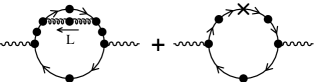
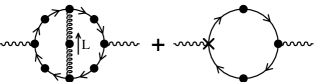
Figure 1: Two-loop contributions. A black dot denotes an effective propagator or vertex. Crosses are HTL counterterms.

More formally, the counterterms automatically arise when we construct the perturbative expansion with effective propagators and vertices rather than with the original propagators and vertices. The effective perturbative expansion is nothing but a reorganization of the usual perturbative expansion. The effective Lagrangian ${\cal L}_{\rm eff}$, which leads to effective propagators and vertices, already includes some one-loop thermal contributions. In order to keep the same theory as that given by the original Lagrangian ${\cal L}$ one has to supplement the effective Lagrangian with counterterms to subtract order by order the loop-corrections already included in the effective Lagrangian so that

$${\cal L}={\cal L}_{\rm eff}+{\cal L}_{\rm c.t.}.$$ (2)

The counterterms are then treated perturbatively and thus appear in the expansion when looking at higher order topologies.

The imaginary part of the retarded vacuum polarization in Eq. (1) can be expressed as a sum over different cuts through the diagrams of Fig. 1. Calculating the cut diagrams with the full complexity of effective propagators and vertices would be a formidable task. To extract only the leading behavior of the two-loop contributions one can make some useful simplifications. This leading contribution arises essentially when a hard momentum flows in the quark loop. This is a consequence of the phase space available, $\int d^{4}p\sim T^{4}$ in the hard region, compared to $g^{4}T^{4}$ for the soft region. Besides that, for soft fermion momentum $P$, the leading contribution should be contained entirely in the one-loop diagram since effective propagators and vertices give the complete behavior at scale $gT$. In the soft quark region, the two-loop diagrams (with associated counterterms) will only give sub-dominant terms while new dominant contributions can occur in the hard quark regime. Concentrating now on the region where the quarks are hard, it is sufficient to use bare vertices rather than effective ones and to keep only the time-like sector of cut fermion propagators, which largely dominates over the space-like sector. To see that, one can compare the behavior of the spectral density $\delta(P^{2})\raise 0.6458pt\hbox{$/$}\kern-5.29999pt\hbox{$P$}={\cal O}(1/p)$ in the time-like region with its behavior $g^{2}T^{2}\raise 0.6458pt\hbox{$/$}\kern-5.29999pt\hbox{$P$}/p^{4}$ in the space-like region when the momentum $p$ is hard. We are therefore led to calculate the graphs of Fig. 2 with time-like cut fermion lines.

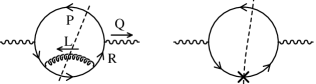
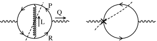
Figure 2: Two-loop contributions in the hard momenta limit. Lines without any dressing denote the hard limit of effective propagators, in which we keep a thermal mass.

With these simplifications, two types of cuts can be distinguished: those going through the gluon propagator and those going only through two fermion propagators. For the moment we ignore the latter because kinematical constraints would require either $P$ and $R$ (see Fig. 2 for the notations) to be time-like and soft (which would lead to a non leading contribution because of the small size of the phase-space), or $P$ to be space-like and hard so that the loop-corrections make these diagrams sub-leading compared to the one-loop result. Cutting through the gluon line, it is convenient to distinguish the space-like $L^{2}$ region from the time-like one. The case of $L^{2}<0$ has been discussed in detail in [5] where it has been shown to contain a new physical process (bremsstrahlung) absent from the one-loop result. No counterterms were needed in this region. From now on, we concentrate on the case $L^{2}>0$. Physically, this region corresponds to Compton and annihilation processes, which are already included in an approximate way in the one-loop calculation of Braaten, Pisarski and Yuan (BPY) [3]. We expect a better approximation of these processes to come out from the evaluation of the two-loop diagrams for the following reason: when evaluating these two-loop graphs, we do not neglect $P$ and $R$ compared to $L$ in the self-energy and vertex corrections since $P$ and $R$ are hard and comparable to $L$. On the contrary, in the HTL approximation “external” momenta $P$ and $R$ are neglected compared to the loop-momentum $L$ in the resummed self-energy corrections to the fermion propagators and in the estimate of the loop correction leading to the effective vertex. We therefore anticipate that in our two-loop calculations, terms of leading order in $L$ in the matrix element will be compensated by counterterms while terms of lower degree in $L$ will lead to new contributions.

The counterterm method described here is not the only way which can be used to calculate the two-loop diagrams while avoiding double counting of thermal corrections. Since, as mentioned above, effective propagators and vertices do not have the correct behavior in the hard limit (more precisely when some of their external momenta are hard and space-like), an alternative way to proceed consists of introducing a cutoff scale intermediate between $gT$ and $T$. In this method, one uses effective propagators and vertices in loops carrying a momentum below the cutoff. Above the cutoff, bare propagators and vertices can be used, and a loop correction must be inserted on the hard propagator. When adding the soft and the hard contributions the cutoff dependence should drop out [7, 12]. This method has been pioneered by Braaten and Yuan in their calculation [13] of the rate of energy loss in a hot plasma, and used later in the calculation of the rate of hard real photon production by a quark-gluon plasma [14, 15]. However it was not followed in [3] where the effective propagators were used up to the hard momentum scale.

A remark is worth making concerning the use of the cutoff method in [14, 15]. Indeed, in these two papers, a bare gluon propagator is used even if the cutoff does not constrain the gluon to be hard. As a consequence of the misuse of the cutoff in this way, [14, 15] missed the important contribution coming from bremsstrahlung [5].

In the following we will obtain analytically the leading $\ln(1/g)$ behavior of the vacuum polarization diagram. The argument of the logarithm is the ratio of a hard scale over a soft scale of order $gT$. Technically, this arises from integrals of type $\int{dp/p}$ or $\int{dl/l}$. To extract this leading behavior one does not need the full details of the effective propagators in the soft region. It is sufficient to approximate the fermion and gluon dispersion relations by their asymptotic forms in the hard region: the error involves ratios of soft scales which are of order $1$ compared to $\ln(1/g)$. Furthermore, only the upper branches (quasi-particles) of the dispersion relations will contribute because the lower branches (collective modes) of both the fermion and the gluon decouple exponentially fast in the hard region and therefore cannot contribute a leading logarithm term. A last technical simplification consists in keeping a constant mass, independent of the momentum, along the dispersion curves: thus we have $m_{{}_{F}}^{2}\sim m_{\rm g}^{2}\sim g^{2}T^{2}$, the exact expression of the thermal masses being irrelevant for the logarithmic behavior.

3 One-loop result

The virtual photon production rate has been calculated at one loop in the effective theory [3]. In their calculation, BPY distinguished three types of terms depending on whether the pole (time-like) part or the cut (space-like) part of the fermionic spectral density is taken into account. We already extracted in [5] the leading logarithmic behavior of the cut-cut contribution and we showed that it should be compared to the $L^{2}<0$ part of the two-loop diagrams. We give now the remaining leading logarithmic part associated to the pole-cut contribution (the pole-pole term does not lead to a logarithm because hard time-like momenta are kinematically suppressed) which describes the Compton and the annihilation processes. From Eq. (11) of [3], taking the hard momentum limit in the integrand, one can easily extract the leading logarithm given by

$$\left.\frac{dN}{d^{4}xdq_{0}d^{3}{\tenimbf q}}\right|_{\rm 1loop} \approx \frac{\alpha^{2}}{12\pi^{4}}\Big{(}\sum_{f}e^{2}_{f}\Big{)}\left(\frac{NC_{{}_{F}}g^{2}T^{2}}{8}\right)\frac{1}{q_{0}^{2}}\ln\left(\frac{q_{0}T}{q_{0}^{2}+m_{{}_{F}}^{2}}\right)\ ,$$ (3)

where $N$ is the number of colors, $C_{{}_{F}}\equiv(N^{2}-1)/2N$, $m_{{}_{F}}^{2}\equiv g^{2}C_{{}_{F}}T^{2}/8$ is the thermal mass of soft quarks and $e_{f}$ is the electric charge of the quark of flavor $f$, in units of electron charge.

For later use, it is convenient to translate this formula into an expression for the photon polarization tensor:

$${\rm Im}\,\Pi^{{}^{RA}}{}_{\mu}{}^{\mu}(q_{0},{\tenimbf 0})\approx-\frac{NC_{{}_{F}}}{8}\frac{e^{2}g^{2}}{4\pi}\Big{(}\sum_{f}e_{f}^{2}\Big{)}q_{0}T\ln\left(\frac{q_{0}T}{q_{0}^{2}+m_{{}_{F}}^{2}}\right)\;.$$ (4)

4 The two-loop calculation

4.1 General expression and the logarithmic behavior

The two-loop expression (without counterterms) has been derived in [5] under the same simplifying assumptions as those used here (hard fermion momenta, no effective vertices). There is was found

$$\!\!\!{\rm Im}\,\Pi^{{}^{RA}}{}_{\mu}{}^{\mu}(q_{0},{\tenimbf q})=-\frac{NC_{{}_{F}}}{2}e^{2}g^{2}\int{{d^{4}P}\over{(2\pi)^{3}}}\int{{d^{4}L}\over{(2\pi)^{3}}}[n_{{}_{F}}(r_{0})-n_{{}_{F}}(p_{0})]$$

$$\times\;[n_{{}_{B}}(l_{0})+n_{{}_{F}}(r_{0}+l_{0})]\delta(P^{2}-m_{{}_{F}}^{2})\delta((R+L)^{2}-m_{{}_{F}}^{2})\epsilon(p_{0})\epsilon(r_{0}+l_{0})$$

$$\times\;\sum\limits_{a=T,L}\rho_{a}(L)P^{a}_{\rho\sigma}(L)\left[{{{\rm Trace}{}^{\rho\sigma}{}_{|_{\rm vertex}}}\over{\overline{R}{}^{2}(\overline{P+L}){}^{2}}}+{{{\rm Trace}{}^{\rho\sigma}{}_{|_{\rm self}}}\over{\overline{R}{}^{2}\overline{R}{}^{2}}}\right]$$ (5)

where $e$ is the electric charge of the quark running in the loop and where the notation $\overline{R}\equiv(r_{0},\sqrt{r^{{2}}+m_{{}_{F}}^{{2}}}\hat{\tenimbf r})$ includes the thermal mass shift on the fermion propagator:

$${{\overline{\raise 0.6458pt\hbox{$/$}\kern-5.29999pt\hbox{$R$}}}\over{\overline{R}}^{2}\pm ir_{0}\varepsilon}={{\overline{\raise 0.6458pt\hbox{$/$}\kern-5.29999pt\hbox{$R$}}}\over R^{2}-m_{{}_{F}}^{2}\pm ir_{0}\varepsilon}.$$ (6)

After contracting over the transverse and longitudinal gluon projectors [16, 17],

$$P^{{}^{T}}_{\rho\sigma}(L)=g_{\rho\sigma}-U_{\rho}U_{\sigma}+{{(L_{\rho}-l_{0}U_{\rho})(L_{\sigma}-l_{0}U_{\sigma})}\over{l^{2}}}$$ (7)

$$P^{{}^{L}}_{\rho\sigma}(L)=-P^{{}^{T}}_{\rho\sigma}(L)+g_{\rho\sigma}-{{L_{\rho}L_{\sigma}}\over{L^{2}}}\;,$$ (8)

where $U\equiv(1,{\tenimbf 0})$ is the 4-velocity of the plasma in its rest frame we arrive at:

$$\!\!\sum\limits_{a=T,L}\rho_{a}(L)P^{a}_{\rho\sigma}(L)\left[{{{\rm Trace}{}^{\rho\sigma}{}_{|_{\rm vertex}}}\over{\overline{R}{}^{2}(\overline{P+L}){}^{2}}}+{{{\rm Trace}{}^{\rho\sigma}{}_{|_{\rm self}}}\over{\overline{R}{}^{2}\overline{R}{}^{2}}}\right]=\sum\limits_{a=T,L}\rho_{a}(L)|{\cal M}_{a}|^{2}$$

$$\approx-4\left[\left(\rho_{{}_{T}}(L)-\rho_{{}_{L}}(L)\right){{4p^{2}(\cos^{2}\theta^{\prime}-1)}\over{\overline{R}{}^{2}(\overline{P+L}){}^{2}}}\left(L^{2}-2{{Q^{2}(Q\cdot L)^{2}}\over{\overline{R}{}^{2}(\overline{P+L}){}^{2}}}\right)\right.$$

$$\qquad+2{{(Q+L)^{2}}\over{\overline{R}{}^{2}(\overline{P+L}){}^{2}}}\left(Q^{2}\rho_{{}_{L}}(L)+L^{2}\rho_{{}_{T}}(L)\right)$$

$$\qquad-2\rho_{{}_{T}}(L)\left(1-2{{(Q\cdot L)^{2}}\over{\overline{R}^{2}(\overline{P+L}){}^{2}}}\left.+{{Q^{2}L^{2}}\over 2}\left[{1\over{(\overline{R}{}^{2})^{2}}}+{1\over{((\overline{P+L}){}^{2})^{2}}}\right]\right)\right]$$ (9)

where $\theta^{\prime}$ is the angle between $\tenimbf r$ and $\tenimbf l$ (or $\tenimbf p$ and $\tenimbf l$ since the virtual photon is static). Unlike in our previous work which dealt with the contribution of the space-like part of the gluon phase space, we consider here the time-like part and use:

$$\rho_{a}(L)=2\pi\epsilon(l_{0})\delta(L^{2}-{\rm Re}\,\Pi_{a}).$$ (10)

Eq. (5) accounts for the cuts shown in Fig. 2. We still have to include the symmetric cut for the vertex diagram and also the diagram with the self-energy correction on the lower line. This will be done simply by multiplying the final result by an overall factor of 2.

Since the external photon is massive, $Q^{2}\sim g^{2}T^{2}$, there does not appear any collinear singularities of the type discussed in [4] and the logarithmic behavior arises only from terms like $\int{dp/p}$ or $\int{dl/l}$. A simple power counting will then allow us to isolate the relevant terms in Eqs. (5) and (9). We can use the following rules

• $\int dp_{0}\,\delta(P^{2}-m_{{}_{F}}^{2})\sim\displaystyle{\frac{1}{p}}\;$,

• $\int dl_{0}\,\delta(L^{2}-{\rm Re}\,\Pi_{a})\displaystyle{\sim\frac{1}{l}}$,

• $\int d\cos\theta^{\prime}\,\delta((R+L)^{2}-m_{{}_{F}}^{2})\sim\displaystyle{\frac{1}{pl}}$,

• $n_{{}_{F}}(r_{0})-n_{{}_{F}}(p_{0})\sim\displaystyle{\frac{q_{0}}{T}}$ since $q_{0}=r_{0}-p_{0}$ is soft,

• $n_{{}_{B}}(l_{0})+n_{{}_{F}}(r_{0}+l_{0})\sim\displaystyle{\frac{T}{l_{0}}}\sim\displaystyle{\frac{T}{l}}$,

to write, ignoring any irrelevant angular integrations,

$${\rm Im}\,\Pi^{{}^{RA}}{}_{\mu}{}^{\mu}\sim e^{2}g^{2}q_{0}\int dp{dl\over l}\sum\limits_{a=T,L}|{\cal M}_{a}|^{2}.$$ (11)

Estimating ${\overline{R}}^{2}\sim 2pq_{0}$ and likewise for ${(\overline{P+L})}^{2}$, we find that only the terms

$$-2\rho_{{}_{T}}\left(1-2{{(Q\cdot L)^{2}}\over{\overline{R}{}^{2}(\overline{P+L}){}^{2}}}\right)=-2\rho_{{}_{T}}\left(1+Q\cdot L\left({1\over\overline{R}^{2}}+{1\over(\overline{P+L}){}^{2}}\right)\right)\;,$$ (12)

leading to

$${\rm Im}\,\Pi^{{}^{RA}}{}_{\mu}{}^{\mu}\sim e^{2}g^{2}q_{0}\int dp{dl}\,\left({\cal O}({1\over p})+{\cal O}({1\over l})\right)$$ (13)

contribute to the leading logarithmic behavior. It has been checked by explicit analysis that all the other terms do not have the proper scaling behavior to give a logarithm. It can be noted here that the relevant terms for the present analysis are totally different from those in the bremsstrahlung case ($L^{2}<0$). This is related to the different behavior of the gluon spectral density in the space-like region and the time-like region for hard momentum. More precisely, in our calculation of the trace using the Feynman gauge, the leading bremsstrahlung terms were all contained in the vertex corrections whereas for Compton and annihilation they appear in the diagrams with self-energy corrections.

To summarize, in order to obtain the leading logarithmic terms for positive $L^{2}$ it is sufficient to calculate

$$\!\!\!{\rm Im}\,\Pi^{{}^{RA}}{}_{\mu}{}^{\mu}(q_{0},{\tenimbf 0})\approx 4NC_{{}_{F}}\ e^{2}g^{2}\int{{d^{4}P}\over{(2\pi)^{3}}}\int{{d^{4}L}\over{(2\pi)^{3}}}[n_{{}_{F}}(r_{0})-n_{{}_{F}}(p_{0})]$$

$$\times\;[n_{{}_{B}}(l_{0})+n_{{}_{F}}(r_{0}+l_{0})]\delta(P^{2}-m_{{}_{F}}^{2})\delta((R+L)^{2}-m_{{}_{F}}^{2})\epsilon(p_{0})\epsilon(r_{0}+l_{0})$$

$$\times\;2\pi\epsilon(l_{0})\delta(L^{2}-{\rm Re}\,\Pi_{T})\left[1+\left(\frac{Q\cdot L}{\overline{R}{}^{2}}+\frac{Q\cdot L}{(\overline{P+L}){}^{2}}\right)\right]$$

$$\qquad\qquad\qquad\ \equiv{\rm Im}\,\Pi_{1}(q_{0},{\tenimbf 0})+{\rm Im}\,\Pi_{2}(q_{0},{\tenimbf 0})$$ (14)

The above decomposition of ${\rm Im}\,\Pi$ into two parts is natural: ${\rm Im}\,\Pi_{1}$ (the term $1$ in the square brackets) is dominated by hard $p$ while the logarithm comes from the $l$ integration; on the other hand, ${\rm Im}\,\Pi_{2}$ (the terms proportional to $Q\cdot L$) is dominated by hard $l$ and it has a logarithm in the $p$ integration, which indicates that we can make different approximations in each of these parts. From the discussion in section 2, we anticipate that ${\rm Im}\,\Pi_{1}$ is a new two-loop contribution while ${\rm Im}\,\Pi_{2}$ should be compensated by counterterms.

4.2 Hard $p$ region (${\rm Im}\,\Pi_{1}$)

Being dominated by hard $p$, we can neglect $m_{{}_{F}}$ in ${\rm Im}\,\Pi_{1}$, and hence we can use the same kinematical approximations as in [5]. Using the $\delta((R+L)^{2})$ function, we get for the angle $\theta^{\prime}$ between ${\tenimbf p}$ and ${\tenimbf l}$:

$$\cos\theta^{\prime}={{(r_{0}+l_{0})^{2}-p^{2}-l^{2}}\over{2pl}}\;.$$ (15)

Additionally, $\cos\theta^{\prime}$ must be kept within $[-1,+1]$, which places some constraints on the phase space. Eq. (15), together with the condition on $\cos\theta^{\prime}$, gives the following inequalities:

$$(l_{0}-l+p_{0}+q_{0}-p)(l_{0}+l+p_{0}+q_{0}+p)\leq 0$$ (16)

$$(l_{0}-l+p_{0}+q_{0}+p)(l_{0}+l+p_{0}+q_{0}-p)\geq 0\;,$$ (17)

with $|p_{0}|=p$. We assume $p$ fixed and hard and solve the inequalities for $l_{0}$ and $l$ which leads to the phase space reduction seen in Fig. 3.

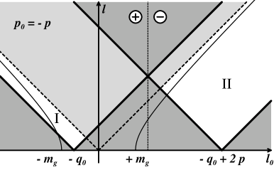
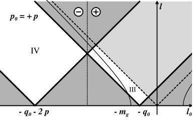
Figure 3: Allowed domains in the $(l_{0},l)$ plane for $p_{0}=\pm p$. The area shaded in dark gray is excluded by the delta functions. The region shaded in light gray is below the light-cone (dotted lines). The thin solid curves are the transverse dispersion curves of the thermalized gluon. The vertical dotted line is the separation between $\epsilon(p_{0})\epsilon(r_{0}+l_{0})=+1$ and $\epsilon(p_{0})\epsilon(r_{0}+l_{0})=-1$.

The different allowed regions in Fig. 3 can be interpreted in terms of physical processes (Fig. 4) determined by the relative signs of the energies $p_{0}$, $l_{0}$ and $r_{0}+l_{0}$. We have Compton processes in regions (I) and (III), quark-antiquark annihilation in region (II), and plasmon decay in region (IV). The symmetry of the integrand in ${\rm Im}\,\Pi_{1}$ with respect to the change of variables $P\leftrightarrow-R-L$, indicates that regions (I) and (III) give equal contributions. Therefore, we will consider one region (I for instance) and multiply the end result by $2$. The domain of integration of Eq. (14) is constrained by the $\delta$ function Eq. (10), which further reduces the allowed phase space to the intersection of the dispersion curves with the regions I to IV. We also note that the longitudinal modes of the gluon cannot give a large logarithm in the momentum integral, since longitudinal modes are exponentially suppressed in the hard region.

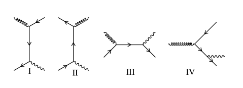
Figure 4: Examples of physical processes included in the phase-space of of Fig. 3. Region I: $p_{0}<0$, $r_{0}+l_{0}<0$: Compton scattering of an antiquark. Region II: $p_{0}<0$, $r_{0}+l_{0}>0$: $q\bar{q}$ annihilation. Region III: $p_{0}>0$, $r_{0}+l_{0}>0$: Compton scattering of a quark. Region IV: $p_{0}>0$, $r_{0}+l_{0}<0$: plasmon decay into $q\bar{q}$ and a photon. For the gluon, we use an approximate dispersion relation, with a constant thermal mass. The quarks being hard need not be effective.

The transverse gluon polarization tensor introduced in Eq. (10) is given by:

$$\Pi_{{}_{T}}(l_{0},l)=3m_{\rm g}^{2}\left[{{x^{2}}\over 2}+{{x(1-x^{2})}\over{4}}\ln\left|{{x+1}\over{x-1}}\right|\right]\;,$$ (18)

where $x\equiv l_{0}/l$. For a time-like gluon, $\Pi_{{}_{T}}(lx,l)$ is a function of $x$ varying slowly between $m_{\rm g}^{2}/2$ and $3m_{\rm g}^{2}/2$. Therefore, at the logarithmic accuracy in the evaluation of Eq. (14), we can take $\Pi_{{}_{T}}\approx m_{\rm g}^{2}$. Making this approximation, we obtain the following expression for ${\rm Im}\,\Pi_{1}$ :

$${\rm Im}\,\Pi_{1}(q_{0},{\tenimbf 0)}\approx-{{8NC_{{}_{F}}e^{2}g^{2}}\over{(2\pi)^{3}}}{q_{0}}\int\limits_{0}^{+\infty}dp\,n^{\prime}_{{}_{F}}(p)\;\int\limits_{-\infty}^{-1}dx$$

$$\qquad\times\int\limits_{{q_{0}}\over{1-x}}^{-{q_{0}}\over{1+x}}dl\,l^{2}\delta(L^{2}-m_{\rm g}^{2})[n_{{}_{B}}(lx)+n_{{}_{F}}(-p+q_{0}+lx)]$$ (19)

where we have used $n_{{}_{F}}(p_{0}+q_{0})-n_{{}_{F}}(p_{0})\approx q_{0}n^{\prime}_{{}_{F}}(p)$. In the normalization, we have taken into account the above mentioned factors of $2$. The integrals can easily be done to logarithmic accuracy and we obtain:

$${\rm Im}\;\Pi_{1}(q_{0},{\tenimbf 0})\approx-{{NC_{{}_{F}}e^{2}g^{2}}\over{4\pi^{3}}}\Big{(}\sum_{f}e^{2}_{f}\Big{)}{q_{0}}T\ln\left(\frac{q_{0}T}{m_{\rm g}^{2}+q_{0}^{2}}\right)\;,$$ (20)

where we have reintroduced the summation over the flavors running in the quark loop. The occurrence of $m_{\rm g}$ indicates that this logarithm cannot be found at one-loop in the HTL scheme since only the thermal fermion mass appears at this level. As we will see later on, this is not compensated by the counterterms. We find that the annihilation process (region II) contributes to ${\rm Im}\;\Pi_{1}$ at leading order $e^{2}g^{2}q_{0}T$, but without a logarithm since $l$ is constrained to be hard in this region (see Fig. 3). Similarly, the plasmon decay process (region IV) can be ignored at the logarithmic accuracy.

4.3 Hard $l$ region (${\rm Im}\,\Pi_{2}$)

In order to calculate ${\rm Im}\,\Pi_{2}$, we follow the same procedure as in the previous section but interchanging the roles of $l$ and $p$. Since ${\rm Im}\,\Pi_{2}$ is dominated by the hard $l$-region, we can neglect the gluon thermal mass. Again we start with the $\delta$ function $\delta((R+L)^{2}-m_{{}_{F}}^{2})$, which provides us with the angle $\theta^{\prime}$ via the relation:

$$\cos\theta^{\prime}={{R^{2}-m^{2}_{{}_{F}}+2r_{0}l_{0}+L^{2}}\over{2rl}}\;.$$ (21)

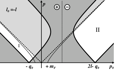
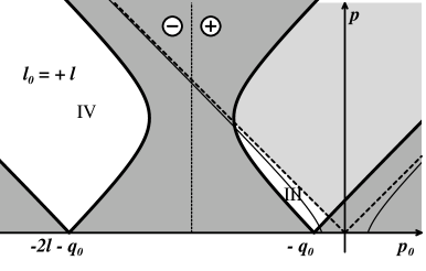
Figure 5: Allowed domains in the $(p_{0},p)$ plane for $l_{0}=\pm l$. The area shaded in dark gray is excluded by the delta function constraints. The areas shaded in light gray are below the light-cone (dotted lines). The thin solid curves are the mass shells of the thermalized quarks. The vertical dotted line is the separation between $\epsilon(l_{0})\epsilon(r_{0}+l_{0})=+1$ and $\epsilon(l_{0})\epsilon(r_{0}+l_{0})=-1$.

As before, we must enforce $-1\leq\cos\theta^{\prime}\leq 1$, which implies the following set of inequalities:

$$(r_{0}-r+l_{0}+l)(r_{0}+r+l_{0}-l)\geq m^{2}_{{}_{F}}$$ (22)

$$(r_{0}-r+l_{0}-l)(r_{0}+r+l_{0}+l)\leq m^{2}_{{}_{F}}\;.$$ (23)

We can further simplify these inequalities and write them as:

$$\sqrt{(p-l)^{2}+m_{{}_{F}}^{2}}\leq l_{0}+r_{0}\ {\rm or}\ l_{0}+r_{0}\leq-\sqrt{(p-l)^{2}+m_{{}_{F}}^{2}}$$ (24)

$$-\sqrt{(p+l)^{2}+m_{{}_{F}}^{2}}\leq l_{0}+r_{0}\leq\sqrt{(p+l)^{2}+m_{{}_{F}}^{2}}\;.$$ (25)

Keeping $l$ hard, the above inequalities lead to a reduction of the allowed domain in the $(p_{0},p)$ plane (see Fig. 5) where the case $l_{0}=l$ and $l_{0}=-l$ have to be distinguished.

As before, the various regions admit a physical interpretation. Regions I and II represent Compton scattering on an antiquark and on a quark respectively, while region III contains quark-antiquark annihilation. Region IV describes quark decay into quark, gluon and photon, but it is not allowed if the initial and final quarks have the same masses. We note also the absence of plasmon decay, which is entirely due to the different approximations made in this section and in the previous one: here we assume $L^{2}=0$ but keep the fermion mass and this forbids the decay of the gluon into a photon and a massive quark-antiquark pair.

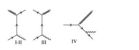
Figure 6: Examples of physical processes included in the phase-space of Fig. 5. Region I: $p_{0}<0$, $r_{0}+l_{0}<0$,$l_{0}<0$: Compton scattering of an antiquark. Region II: $p_{0}>0$, $r_{0}+l_{0}>0$,$l_{0}<0$: Compton scattering of a quark. Region III: $p_{0}<0$, $r_{0}+l_{0}>0$,$l_{0}>0$: $q\bar{q}$ annihilation. Region IV: $p_{0}<0$, $r_{0}+l_{0}<0$,$l_{0}>0$: quark decay into $qg$ and a photon. For the quarks, we use an approximate dispersion relation, with a constant thermal mass. The gluon being hard is treated as a bare gluon.

The change of variables $P\leftrightarrow-R-L$ in the $Q\cdot L/(\overline{P+L})^{2}$ term in ${\rm Im}\,\Pi_{2}$ allows us to write:

$$\!\!\!{\rm Im}\,\Pi_{2}(q_{0},{\tenimbf q})\approx-8NC_{{}_{F}}e^{2}g^{2}\int{{d^{4}P}\over{(2\pi)^{3}}}\int{{d^{4}L}\over{(2\pi)^{3}}}[n_{{}_{F}}(r_{0})-n_{{}_{F}}(p_{0})]$$

$$\times\;[n_{{}_{B}}(l_{0})+n_{{}_{F}}(r_{0}+l_{0})]\delta(\overline{P}^{2})\delta((\overline{R+L})^{2})\epsilon(p_{0})\epsilon(r_{0}+l_{0})$$

$$\times\;2\pi\epsilon(l_{0})\delta(L^{2})\frac{Q\cdot L}{\overline{R}{}^{2}}$$ (26)

This integral can be evaluated relatively easily. Consider, for example, region III ($l_{0}=l,\ p_{0}<0,\ r_{0}+l_{0}>0,\ i.e.\ q\bar{q}$ annihilation). For $l$ fixed and hard, the fermion dispersion curve $p_{0}\approx-\omega_{p}=\sqrt{p^{2}+m_{{}_{F}}^{2}}$ intersects the boundary of the region at

$$p_{\rm min}\approx{|q_{0}^{2}-m_{{}_{F}}^{2}|\over 2q_{0}},\qquad p_{\rm max}\approx l$$ (27)

so that, after doing all angular integrations and using the $\delta$ functions, one finds

$${\rm Im}\,\Pi^{{}^{III}}_{2} \approx -NC_{{}_{F}}\frac{e^{2}g^{2}}{(2\pi)^{3}}q_{0}\int\limits_{0}^{\infty}ldl\,\int\limits_{p_{\rm min}}^{p_{\rm max}}{pdp\over\omega_{p}}$$ (28)

$$\quad\times[n_{{}_{B}}(l)+n_{{}_{F}}(l-\omega_{p})]\ {[n_{{}_{F}}(\omega_{p})-n_{{}_{F}}(\omega_{p}-q_{0})]\over 2q_{0}\omega_{p}-q_{0}^{2}}$$

$$\approx -{NC_{{}_{F}}\over 2}\frac{e^{2}g^{2}}{(2\pi)^{3}}\int\limits_{0}^{\infty}ldl\ \int\limits_{|q_{0}^{2}+m_{{}_{F}}^{2}|\over 2q_{0}}^{l}{d\omega_{p}}$$

$$\quad\times[n_{{}_{B}}(l)+n_{{}_{F}}(l-\omega_{p})]\ {[n_{{}_{F}}(\omega_{p})-n_{{}_{F}}(\omega_{p}-q_{0})]\over\omega_{p}-q_{0}/2}$$

We can neglect $\omega_{p}$ in front of $l$ in the term $n_{{}_{F}}(l-\omega_{p})$, and the two integrals decouple. The integral over $l$ leads to the usual hard thermal factor ${\pi^{2}T^{2}}/{4}$ while the integral over $p$ yields a logarithmic factor $\ln({q_{0}T/m_{{}_{F}}^{2}})$. Using the same method, one finds that the contribution of the sector $l_{0}=-l$ in Fig. 5 is similar to Eq. (28) so that, to the required accuracy, Eq. (26) leads to

$${\rm Im}\,\Pi_{2}(q_{0},{\tenimbf 0})\approx-\frac{NC_{{}_{F}}}{8}\frac{e^{2}g^{2}}{4\pi}\Big{(}\sum_{f}e_{f}^{2}\Big{)}q_{0}T\ln\left({q_{0}T\over m_{{}_{F}}^{2}}\right)$$ (29)

where we have included the charge factor of the quarks. The normalization factor takes into account the contribution of all the ways of cutting through the photon polarization diagrams.

5 Counterterms

We have calculated the two-loop diagrams using various approximations. As a consequence, in order to be consistent, we have to use the same approximation when evaluating the counterterms. In the appendix, we show that the complete computation of the counterterms gives the same logarithmic contribution as the simplified version of the counterterm diagrams we discuss in this section.

The simplified version of the vertex counterterm and the self-energy counterterm are depicted on the right of Fig. 2.

Their general structure is as in Eq. (5) but the integrals have now to be evaluated using the HTL approximations, namely $L$ hard with $L^{2}=0$ and $P$ and $R$ neglected with respect to $L$ with, as before, the notation $\overline{P}=(p_{0},\sqrt{p^{2}+m_{{}_{F}}^{2}}\hat{\tenimbf p})$, $\overline{R}=(p_{0}+q_{0},\sqrt{p^{2}+m_{{}_{F}}^{2}}\hat{\tenimbf p})$. This implies $(\overline{R+L})^{2}\approx 2{R}\cdot L$. One then writes

$${\rm Im}\,\Pi(q_{0},{\tenimbf 0})|_{\rm ct}\approx\frac{NC_{{}_{F}}}{2}e^{{2}}g^{{2}}\int{{d^{4}P}\over{(2\pi)^{3}}}\int{{d^{4}L}\over{(2\pi)^{3}}}[n_{{}_{F}}(r_{0})-n_{{}_{F}}(p_{0})]$$

$$\qquad\qquad\qquad\qquad\times\;[n_{{}_{B}}(l_{0})+n_{{}_{F}}(l_{0})]\epsilon(p_{0})\delta(\overline{P}^{2})\delta(2R\cdot L)\delta(L^{2})$$

$$\qquad\qquad\qquad\qquad\times\;2\pi g_{\rho\sigma}\left[{{{\rm Trace^{\rho\sigma}_{{}_{HTL}}}{|_{\rm vertex}}}\over{(2P\cdot L)\overline{R}{}^{2}}}+{{{\rm Trace^{\rho\sigma}_{{}_{HTL}}}{|_{\rm self}}}\over{\overline{R}{}^{2}\overline{R}{}^{2}}}\right]$$ (30)

where the traces can be evaluated using the Feynman gauge for the gluon. In this equation we make use of $r_{0}+l_{0}\approx l_{0}$ so that some $\epsilon$-functions drop out.

For the vertex we find simply in the HTL approximation

$$g_{\rho\sigma}{\rm Trace^{\rho\sigma}_{{}_{HTL}}}|_{\rm vertex}\approx 32\ \overline{R}.L\ \overline{P}.L=0\;.$$ (31)

Hence the vertex counterterm is vanishing within the approximation used. This is not a general result but a consequence of using the Feynman gauge.

The self energy counterterm is non vanishing and we find

$$g_{\rho\sigma}{\rm Trace^{\rho\sigma}_{{}_{HTL}}}|_{\rm self} = 16\ (2(\overline{P}\cdot\overline{R})(\overline{R}\cdot L)-\overline{R}^{2}\overline{P}\cdot L)$$ (32)

$$\approx 16\ \overline{R}^{2}\ Q\cdot L\ .$$

In the last line, we have neglected terms which are suppressed by inverse powers of $p$ at large $p$ which cannot contribute to a logarithmic factor in the $p$ integration. Plugging this expression in Eq. (30) and comparing to Eq. (26), we find that these two equations coincide at the logarithmic level, except for the sign. Indeed, their sum receives a contribution only when $p$ is hard and therefore does not have a logarithmic behavior. One concludes that, to logarithmic accuracy,

$${\rm Im}\,\Pi_{2}(q_{0},{\tenimbf 0})+{\rm Im}\,\Pi(q_{0},{\tenimbf 0})|_{\rm ct}\simeq 0$$ (33)

so that, as expected, the counterterms cancel the two-loop contribution arising from the hard $L$ phase-space.

6 The total two-loop contribution

We summarize in this section the complete results of the calculation of the virtual photon rate up to two loops in the effective perturbative expansion. We have to collect the following pieces: the one-loop result of [3] given in Eq. 3, the two-loop bremsstrahlung contribution derived in [5] and finally the contribution of the Compton and annihilation processes we have calculated in the previous sections of the present paper. Adding all three contributions, we obtain to leading order in $\ln(1/g)$:

$$\frac{dN}{d^{4}xdq_{0}d^{3}{\tenimbf q}} \approx \frac{\alpha^{2}}{3\pi^{6}q_{0}^{2}}\Big{(}\sum_{f}e^{2}_{f}\Big{)}\left(\frac{NC_{{}_{F}}g^{2}T^{2}}{8}\right)$$ (34)

$$\times\left\{\frac{\pi^{2}m_{{}_{F}}^{2}}{4q_{0}^{2}}\ln\left({{T^{2}}\over{m^{2}_{{}_{F}}}}\right)+\frac{3m^{2}_{\rm g}}{q_{0}^{2}}\ln\left(\frac{T^{2}}{m_{\rm g}^{2}}\right)\right.$$

$$\left.+\frac{\pi^{2}}{4}\ln\left(\frac{q_{0}T}{m^{2}_{{}_{F}}+q_{0}^{2}}\right)+2\ln\left(\frac{q_{0}T}{m_{\rm g}^{2}+q_{0}^{2}}\right)\right\}\;.$$

The term in ${m_{{}_{F}}^{2}}/{q_{0}^{2}}$ arises from the cut-cut term in the one-loop calculation while the term in ${m^{2}_{\rm g}}/{q_{0}^{2}}$ describes the bremsstrahlung coming from the two-loop diagrams. The last line combines the pole-cut contribution at one-loop, Eq. (3), as well as the $L^{2}>0$ pieces at two-loop, Eqs. (20), (29), and the associated counterterms Eq. (33). In the above equation, the choice of hiding some powers of $gT$ in thermal masses is somewhat arbitrary. Nevertheless, it should be noted that, even if the four terms have the same order of magnitude when $q_{0}$ is soft, two of them are proportional to $e^{2}g^{4}$ and therefore would be obtained only at three loops in the naive perturbative expansion.

If we consider the leading term in an expansion in powers of $g$ at fixed $q_{0}$ (which is precisely what one is doing in the bare theory), we should be able to recover the results of two-loop bare calculations performed by [8]. Taking this limit in Eq. (34), we find:

$$\frac{dN}{d^{4}xdq_{0}d^{3}{\tenimbf q}}\approx\frac{\alpha^{2}}{3\pi^{6}q_{0}^{2}}\Big{(}\sum_{f}e^{2}_{f}\Big{)}\left(\frac{NC_{{}_{F}}g^{2}T^{2}}{8}\right)(\frac{\pi^{2}}{4}+2)\ln({T\over q_{0}})\;.$$ (35)

which is precisely the result found in [8]. One may notice that, had we kept only the terms calculated by BPY [3], the $g\to 0$ expansion of Eq. (34) would not reproduce the complete bare result.

One may also wonder what happens when considering the ultra-soft photon limit, $q_{0}\ll m_{{}_{F}}$ or $q_{0}\ll m_{\rm g}$, for which the pole-cut contributions in Eq. (34) seems completely wrong. A glance at Fig. 3 and Fig. 5 shows that, in that case, the intersection of the dispersion curves with the boundaries of the physical regions are pushed to hard $l$ or $p$ values so that no logarithm is generated. This is reflected in Eq. (34), where some logarithms become small and eventually negative when $q_{0}$ goes to zero, indicating that the terms we considered no longer exhibit a large logarithmic factor. More technically, in the case of Eq. (20) for example, the integration generates terms such as

$$\ln(1-\exp(-\frac{q_{0}^{2}+m_{\rm g}^{2}}{2q_{0}T}))$$

which reduce to the usual logarithm for the generic case $q_{0}\sim m_{\rm g}\sim gT$ but which lead to an exponentially suppressed factor when $q_{0}\ll m_{\rm g}^{2}/T$.

For completeness, we briefly mention here the case of thermal production of hard or very hard real photon ($q_{0}\geq T$) [14, 15]. It was found in the 2-loop approximation [5] that, as in the case of soft virtual photon production, leading contributions arose from the space-like part of the gluon spectral density ($L^{2}<0$) associated to the bremsstrahlung process as well as to $q-\bar{q}$ annihilation with scattering. To complete the calculation, the time-like ($L^{2}\geq 0$) part should be considered. However it is not necessary to do the calculation using the counterterm method advocated above since in the published works [14, 15] the two-loop contribution has already been included using the cutoff method. The final result contains a factor $\ln(q_{0}T/m_{{}_{F}}^{2})$ similar to those of Eq. (34).

7 Conclusions

In this work, we complete the study of soft static lepton pair production in a quark-gluon plasma, in the two-loop approximation of the effective perturbative expansion. At one loop, the result shows a logarithmic sensitivity to hard momenta in the loop. Since the extrapolation of hard thermal loops is not accurate enough in the hard space-like region, we anticipate that the one-loop approximation may not yield the complete result at the leading order in the expansion in powers of the coupling constant. We should then consider two-loop diagrams, and an explicit calculation shows that, indeed, they give a contribution at leading order. Two types of terms can be distinguished, which are associated with different physical processes:

(i) two-loop leading corrections to processes already included at one-loop. They are the Compton and annihilation production of the virtual photon, which are calculated incompletely at the one-loop level.

(ii) New processes, not contained in the one-loop approximation, namely the bremsstrahlung production of the photon. This was studied elsewhere [5].

Dealing with two-loop diagrams in the HTL resummed theory requires some care. Two approaches are possible. One can use the cutoff method where the two-loop corrections are taken into account only above some cutoff value of the loop momentum. But this is not enough to evaluate the two-loop diagrams using bare propagators and vertices only. On the contrary, effective propagators and vertices are necessary when appropriate. Failing to do this, one could miss the “new” contributions referred to above.

As an alternative to the cutoff method, one can construct the perturbative expansion from the effective Lagrangian, and counterterms must then be included to avoid double counting. These are crucial to correctly calculate the physical processes which appear at different orders of the loop expansion of the effective theory. This is the approach advocated in this work.

Since the new production mechanism of virtual photon at two-loop order shows a logarithmic sensitivity to hard space-like momenta in the loop, it cannot be claimed that our result is complete, for the same reason that the one-loop prediction could not be trusted. The contribution of three-loop diagrams should be considered. However, since in the present calculation there is no physical process that would arise at four loops or more in the bare theory, leading contributions coming from more than three loops are not expected.

Appendix A Counterterms

A.1 Preliminaries

In this appendix we give the exact evaluation of the counterterms. We show that the logarithmic behavior coincides with those found in the paper using the simplified version of the counterterm diagrams. The result according to which the HTL part of the effective vertices does not modify the calculation of the logarithmic part is to be expected on the basis of a quite general argument. Indeed, we know that the HTL correction to the $q\bar{q}\gamma$ vertex behaves like:

$$e(gT)^{2}\int{d\Omega_{\tenimbf l}}{{\hat{\raise 0.6458pt\hbox{$/$}\kern-5.29999pt\hbox{$L$}}\hat{L}^{\mu}}\over{(P\cdot\hat{L})(R\cdot\hat{L})}}\;,$$ (36)

where $L\equiv(1,\hat{\tenimbf l})$ and where $P$ and $R$ are the momenta of the quark and of the antiquark. This means that this HTL correction has a very different scaling behavior when $P$ and $R$ become hard, compared to the bare part of the effective vertex (which is independent of $P$ and $R$). As a consequence, we do not expect a contribution to the logarithmic part from the HTL correction to the vertices. This is what we check explicitly in the following.

To calculate exactly the counterterms of Fig. 1, we follow [3], where the authors relate the imaginary part of the effective vertex to that of the effective propagator, in order to write the final result in terms of the propagator spectral density only. In this paragraph, we define some notations, and some useful formulae.

The effective propagator can be written as:

$${}^{*}{\cal S}(p_{0},{\tenimbf p}) = \sum_{\tau=\pm 1}\frac{\hat{\raise 0.6458pt\hbox{$/$}\kern-5.29999pt\hbox{$P$}}_{\tau}}{2D_{\tau}(p,p_{0}/p)}$$

$${\rm with}\qquad D_{\tau}(p,x) \equiv \frac{1}{p}[p^{2}(x-\tau)-m_{{}_{F}}^{2}\ tau+m_{{}_{F}}^{2}(\tau x-1)Q_{0}(x)]\;,$$ (37)

where $\hat{\raise 0.6458pt\hbox{$/$}\kern-5.29999pt\hbox{$P$}}_{\tau}\equiv\gamma^{o}-\tau\mbox{\boldmath$\gamma$}\cdot{\hat{\tenimbf p}}$, and $Q_{0}(x)\equiv\frac{1}{2}\ln(({x+1})/({x-1}))$ is the first Legendre function. The presence of Legendre functions in the vertex and the propagator allows us to relate the imaginary part of the vertex (or the imaginary part of the product of a propagator with a vertex) to the imaginary part of the propagator. The spectral density of a quark and the imaginary part of the product of a vertex with a propagator are given by:

$$\!\!\!\!\!\rho_{\tau}(p,x)=-2{\rm Im}\frac{1}{D_{\tau}(p,x)}=\frac{p^{2}(x^{2}-1)}{2m_{{}_{F}}^{2}}[\delta(px-\omega_{\pm}(p))+\delta(px+\omega_{\mp}(p))]$$

$$\qquad\qquad\qquad\qquad\qquad\qquad+\beta_{\pm}(p,x)\theta(1-x^{2})\;,$$ (38)

$${\rm Im}\left(\frac{Q_{0}(x)}{D_{\tau}(p,x)}\right)=\frac{1}{2}\left(\frac{p^{2}(x-\tau)-m_{{}_{F}}^{2}\tau}{m_{{}_{F}}^{2}(\tau x-1)}\right)\rho_{\tau}(p,x)$$ (39)

with

$$\beta_{\pm}(p,x)=\frac{(m_{{}_{F}}^{2}/2p^{3})(1\mp x)}{\left(x\mp 1-(m_{{}_{F}}/p)^{2}[Q_{0}(x)\mp Q_{1}(x)]\right)^{2}+[(\pi m_{{}_{F}}^{2}/2p^{2})(1\mp x)]^{2}}$$ (40)

where $Q_{1}(x)\equiv xQ_{0}(x)-1$ is the second Legendre function, and $\omega_{\pm}(p)$ are the solution of the dispersion equation $D_{\tau}(p,\omega_{\pm}(p)/p)=0$.

We need also a formula giving the imaginary part of the product of two vertices and a propagator, given by:

$${\rm Im}\;\left(\frac{Q_{0}^{2}(x)}{D_{\tau}(p,x)}\right)=\frac{p\;{\rm Im}Q_{0}(x)}{m_{{}_{F}}^{2}(\tau x-1)}-\frac{1}{2}\left(\frac{p^{2}(x-\tau)-m_{{}_{F}}^{2}\tau}{m_{{}_{F}}^{2}(\tau x-1)}\right)^{2}\rho_{\tau}(p,x)$$ (41)

where in the retarded prescription ($x\rightarrow x+i\epsilon$):

$${\rm Im}Q_{0}(x)=-\frac{\pi}{2}\theta(1-x^{2})\;.$$ (42)

A.2 Vertex counterterms

There are two counterterms diagrams associated with the 2-loop vertex diagram: one is shown in the lower right corner of Fig. 1 and the other one with the counterterm in place of the other loop. In what follows, we denote by $-R$ the momenta circulating in the upper quark of the diagram of Fig. 1 and $P$ to be the momenta of the lower quark.

Applying the previous formulae, and following [18], we get:

$$\left.\frac{dN}{d^{4}xdq_{0}d^{3}{\tenimbf q}}\right|_{\rm vertex}=\frac{4N(\sum\nolimits_{f}e_{f}^{2})}{3\pi^{4}}\frac{\alpha^{2}}{q_{0}^{2}}\int\limits_{0}^{+\infty}p^{2}dp\int\limits_{-\infty}^{+\infty}dp_{0}\int\limits_{-\infty}^{+\infty}dr_{0}\;n_{{}_{F}}(p_{0})n_{{}_{F}}(r_{0})$$

$$\times\;\delta(q_{0}-p_{0}-r_{0})\left\{2\left(1-\frac{p_{0}^{2}-r_{0}^{2}}{2q_{0}p}\right)^{2}\rho_{+}(P)\rho_{-}(R)\right.$$

$$-\left(1-\frac{p_{0}^{2}-r_{0}^{2}}{2q_{0}p}\right)\rho_{+}(P)\rho_{-}(R)$$

$$+2\left(1+\frac{p_{0}^{2}-r_{0}^{2}}{2q_{0}p}\right)^{2}\rho_{-}(P)\rho_{+}(R)-\left(1-\frac{p_{0}^{2}-r_{0}^{2}}{2q_{0}p}\right)\rho_{-}(P)\rho_{+}(R)$$

$$+\left(1+\frac{p_{0}^{2}+r_{0}^{2}-2p^{2}-2m_{{}_{F}}^{2}}{2q_{0}p}\right)^{2}\rho_{+}(P)\rho_{+}(R)$$

$$-\left(1+\frac{p_{0}^{2}+r_{0}^{2}-2p^{2}-2m_{{}_{F}}^{2}}{2q_{0}p}\right)\rho_{+}(P)\rho_{+}(R)$$

$$+\left(1-\frac{p_{0}^{2}+r_{0}^{2}-2p^{2}-2m_{{}_{F}}^{2}}{2q_{0}p}\right)^{2}\rho_{-}(P)\rho_{-}(R)$$

$$-\left(1-\frac{p_{0}^{2}+r_{0}^{2}-2p^{2}-2m_{{}_{F}}^{2}}{2q_{0}p}\right)\rho_{-}(P)\rho_{-}(R)$$

$$+\theta(p^{2}-p_{0}^{2})\frac{m_{{}_{F}}^{2}}{8pq_{0}^{2}}(1-x^{2})[(1+x)\rho_{+}(R)+(1-x)\rho_{-}(R)]$$

$$\left.+\theta(p^{2}-r_{0}^{2})\frac{m_{{}_{F}}^{2}}{8pq_{0}^{2}}(1-\left(\frac{r_{0}}{p}\right)^{2})[(1+\frac{r_{0}}{p})\rho_{+}(P)+(1-\frac{r_{0}}{p})\rho_{-}(P)]\right\}$$ (43)

Since we want to look for possible double counting in Compton and annihilation processes, we must keep at least one time-like quark momentum ($R^{2}\geq 0$ or $P^{2}\geq 0$). By symmetry, we can limit ourselves to one of these two regions, and multiply the end result by a factor of $2$. Doing the logarithmic approximation (i.e taking $\beta_{\pm}(p,x)\approx{m_{{}_{F}}^{2}}/{2p^{3}(1\mp x)}$, ….), we deduce that the vertex counterterm vanishes at the level of approximation:

$$\left.\frac{dN}{d^{4}xdq_{0}d^{3}{\tenimbf q}}\right|_{\rm vertex}\mathrel{\mathop{\kern 0.0pt\approx}\limits_{{\rm log}}}0\;,$$ (44)

which is equivalent to the result found using the simplified version of the counterterm diagram.

A.3 Propagator counterterms

Making use of the same tools, we can calculate the counterterm diagram associated with the self-energy correction (diagram in the upper right corner of Fig. 1, with the other symmetric diagram where the counterterm insertion is on the lower quark propagator).

Now, the relevant region of phase-space that we want to consider is the region where the line having a counterterm insertion is space-like while the other one is time-like. This is a consequence of limiting ourselves to the cut passing through the self energy insertion in the two loops diagram.

After a lengthy but direct calculation we get (including the two possible diagrams of counterterms insertion):

$$\left.\frac{dN}{d^{4}xdq_{0}d^{3}{\tenimbf q}}\right|_{\rm self}=\frac{4N(\sum\nolimits_{f}e_{f}^{2})}{3\pi^{4}}\frac{\alpha^{2}}{q_{0}^{2}}\int\limits_{0}^{+\infty}p^{2}dp\int\limits_{-\infty}^{+\infty}dp_{0}\int\limits_{-\infty}^{+\infty}dr_{0}\;n_{{}_{F}}(p_{0})n_{{}_{F}}(r_{0})$$

$$\times\;\delta(q_{0}-p_{0}-r_{0})\theta(p^{2}-p_{0}^{2})$$

$$\times\left\{2\left(1-\frac{p_{0}^{2}-r_{0}^{2}}{2q_{0}p}\right)^{2}\left[-\frac{p^{2}}{2}\frac{\partial}{\partial p}\left(\frac{\beta_{+}(P)}{p}\right)-\beta_{+}(P)\right]\Delta_{-}(R)\right.$$

$$+2\left(1+\frac{p_{0}^{2}-r_{0}^{2}}{2q_{0}p}\right)\left[-\frac{p^{2}}{2}\frac{\partial}{\partial p}\left(\frac{\beta_{-}(P)}{p}\right)-\beta_{-}(P)\right]\Delta_{+}(R)$$

$$+\left(1+\frac{p_{0}^{2}+r_{0}^{2}-2p^{2}-2m_{{}_{F}}^{2}}{2q_{0}p}\right)^{2}\left[-\frac{p^{2}}{2}\frac{\partial}{\partial p}\left(\frac{\beta_{+}(P)}{p}\right)-\beta_{+}(P)\right]\Delta_{+}(R)$$

$$+\left(1-\frac{p_{0}^{2}+r_{0}^{2}-2p^{2}-2m_{{}_{F}}^{2}}{2q_{0}p}\right)^{2}\left[-\frac{p^{2}}{2}\frac{\partial}{\partial p}\left(\frac{\beta_{-}(P)}{p}\right)-\beta_{-}(P)\right]\Delta_{-}(R)$$

$$-\frac{m_{{}_{F}}^{2}}{8pq_{0}^{2}}(1-x^{2})[(1+x)\Delta_{+}(R)+(1-x)\Delta_{-}(R)]$$

$$+2\frac{p}{q_{0}}x(x-1)\left(1-\frac{p_{0}^{2}-r_{0}^{2}}{2q_{0}p}\right)\rho_{+}(P)\Delta_{-}(R)$$

$$-2\frac{p}{q_{0}}x(x+1)\left(1+\frac{p_{0}^{2}-r_{0}^{2}}{2q_{0}p}\right)\rho_{+}(P)\Delta_{+}(R)$$

$$-\frac{p}{q_{0}}(x^{2}-1)\left(1+\frac{p_{0}^{2}+r_{0}^{2}-2p^{2}-2m_{{}_{F}}^{2}}{2pq_{0}}\right)\beta_{+}(P)\Delta_{+}(R)$$

$$\left.+\frac{p}{q_{0}}(x^{2}-1)\left(1-\frac{p_{0}^{2}+r_{0}^{2}-2p^{2}-2m_{{}_{F}}^{2}}{2pq_{0}}\right)\beta_{-}(P)\Delta_{-}(R)\right\}$$ (45)

where $x\equiv{p_{0}}/{p}$ and ${\partial}/{\partial p}$ is the partial derivative with respect to $p$ at constant $x$, and where $\Delta_{\pm}(P)$ is the time-like part of the spectral density in Eq. (39), which can be approximated to logarithmic accuracy by $\delta(p_{0}\mp\omega_{+}(p))$ (i.e. the residue of the pole is approximated by $1$, which is its value at large momentum).

Finally, to logarithmic accuracy, we get:

$$\left.\frac{dN}{d^{4}xdq_{0}d^{3}{\tenimbf q}}\right|_{\rm self}\approx\frac{N}{12\pi^{4}}\Big{(}\sum_{f}e^{2}_{f}\Big{)}\frac{\alpha^{2}m_{{}_{F}}^{2}}{q_{0}^{2}}\ln\left(\frac{q_{0}T}{q_{0}^{2}+m_{{}_{F}}^{2}}\right)\;.$$ (46)

References

- [1] E. Braaten, R.D. Pisarski, Nucl. Phys. B 337, 569 (1990).
- [2] J. Frenkel, J.C. Taylor, Nucl. Phys. B 334, 199 (1990).
- [3] E. Braaten, R.D. Pisarski, T.C. Yuan, Phys. Rev. Lett. 64, 2242 (1990).
- [4] P. Aurenche, F. Gelis, R. Kobes, E. Petitgirard, Z. Phys. C 75, 315 (1997).
- [5] P. Aurenche, F. Gelis, R. Kobes, H. Zaraket, Phys. Rev D 58, 085003 (1998).
- [6] H. Zaraket, hep-ph/9810246, in proceedings of the 5th Thermal Field Theory workshop (hep-ph/9811469), Regensburg, Aug. 1998, U. Heinz editor.
- [7] F. Gelis, Thèse de doctorat, Université de Savoie (1998).
- [8] T. Altherr, P. Aurenche, Z. Phys. C 45, 99 (1989).
- [9] E. Braaten, Private communication.
- [10] H.A. Weldon, Phys. Rev. D 28, 2007 (1983).
- [11] C. Gale, J.I. Kapusta, Nucl. Phys. B 357, 65 (1991).
- [12] F. Gelis, hep-ph/9809380, in proceedings of the 5th Thermal Field Theory workshop (hep-ph/9811469), Regensburg, Aug. 1998, U. Heinz editor.
- [13] E. Braaten, T.C. Yuan, Phys. Rev. Lett. 66, 2183 (1991).
- [14] R. Baier, H. Nakkagawa, A. Niegawa, K. Redlich, Z. Phys. C 53, 433 (1992).
- [15] J.I. Kapusta, P. Lichard, D. Seibert, Phys. Rev. D 44, 2774 (1991).
- [16] H.A. Weldon, Phys. Rev. D 26, 1394 (1982).
- [17] N.P. Landsman, Ch.G. van Weert, Phys. Rep. 145, 141 (1987).
- [18] P. Aurenche, T. Becherrawy, E. Petitgirard, Preprint ENSLAPP-A-452/93, hep-ph/9403320 (unpublished) .