Measurement of Neutrino Oscillation by the K2K Experiment

Abstract

We present measurements of $\nu_{\mu}$ disappearance in K2K, the KEK to Kamioka long-baseline neutrino oscillation experiment. One hundred and twelve beam-originated neutrino events are observed in the fiducial volume of Super-Kamiokande with an expectation of $158.1^{+9.2}_{-8.6}$ events without oscillation. A distortion of the energy spectrum is also seen in 58 single-ring muon-like events with reconstructed energies. The probability that the observations are explained by the expectation for no neutrino oscillation is $0.0015\%$ ($4.3\sigma$). In a two flavor oscillation scenario, the allowed $\Delta m^{2}$ region at $\sin^{2}2\theta=1$ is between $1.9$ and $3.5\times 10^{-3}$ $\rm eV^{2}$ at the 90 % C.L. with a best-fit value of $2.8\times 10^{-3}$ $\rm eV^{2}$.

I Introduction

The oscillation of $\nu_{\mu}$ neutrinos into other neutrino flavors is now well established. By using the angle and energy distribution of atmospheric neutrinos, the Super-Kamiokande collaboration has measured the parameters of oscillation and observed the sinusoidal disappearance signature predicted by oscillations Ashie et al. (2005, 2004). The K2K collaboration has previously reported evidence of neutrino oscillations in a man-made neutrino beam which was directed 250 km across Japan Ahn et al. (2003); Aliu et al. (2005).

For neutrinos of a few GeV, the dominant oscillation is between $\nu_{\mu}$ and $\nu_{\tau}$ flavor states and two-flavor oscillations suffice to describe and analyze the data. In the two-flavor neutrino oscillation framework the probability that a neutrino of energy $E_{\nu}$ with a flavor state $\nu_{\mu}$ will later be observed in the $\nu_{\tau}$ flavor eigenstate after traveling a distance $L$ in vacuum is:

$$P(\nu_{\mu}\rightarrow\nu_{\tau})=\sin^{2}2\theta\sin^{2}{\Big{(}}\frac{1.27\Delta m^{2}(\textrm{eV}^{2})L(\textrm{km})}{E_{\nu}(\textrm{GeV})}\Big{)},$$ (1)

where $\theta$ is the mixing angle between the mass eigenstates and the flavor eigenstates and $\Delta m^{2}$ is the difference of the squares of the masses of the mass eigenstates.

The KEK to Kamioka long-baseline neutrino oscillation experiment (K2K) Ahn et al. (2001) uses an accelerator-produced beam of nearly pure $\nu_{\mu}$ with a neutrino flight distance of 250 km to probe the same $\Delta m^{2}$ region as that explored with atmospheric neutrinos. The neutrinos are measured first by a suite of detectors located approximately 300 meters from the proton target and then by the Super-Kamiokande (SK) detector 250 km away. The near detector complex consists of a 1 kiloton water Cherenkov detector (1KT) and a fine grained detector system. SK is a 50 kiloton water Cherenkov detector, located 1000 m underground Fukuda et al. (2003).

The K2K experiment is designed to measure neutrino oscillations using a man-made beam with well controlled systematics, complementing and confirming the measurement made with atmospheric neutrinos. In this paper we report a complete description of the observation of neutrino oscillations in the K2K long-baseline experiment, and present a measurement of the $\Delta m^{2}$ and mixing angle parameters.

Neutrino oscillation causes both a suppression in the total number of $\nu_{\mu}$ events observed at SK and a distortion of the measured energy spectrum compared to that measured at the production point. Therefore, all of the beam-induced neutrino events observed within the fiducial volume of SK are used to measure the overall suppression of flux. In addition, in order to study the spectral distortion, the subset of these events for which the incoming neutrino energy can be reconstructed are separately studied.

If the neutrino interaction which takes place at SK is a charged-current (CC) quasi-elastic(QE)($\nu_{\mu}+n\rightarrow\mu+p$) the incoming neutrino energy can be reconstructed using two-body kinematics, and the spectral distortion studied. At the energy of the K2K experiment typically only the muon in this reaction is energetic enough to produce Cherenkov light and be detected at SK but kinematics of the muon alone are enough to reconstruct the energy for these events.

In order to select the charged-current (CC) quasi-elastic  (QE) events in the data sample, one-ring events identified as a muon ($1R\mu$) are chosen which have a high fraction of CC-QE at the K2K energy. For these events, the energy of the parent neutrino can be calculated by using the observed momentum of the muon, assuming QE interactions, and neglecting Fermi momentum:

$$E_{\nu}^{\rm rec}=\frac{m_{N}E_{\mu}-m^{2}_{\mu}/2}{m_{N}-E_{\mu}+P_{\mu}\cos\theta_{\mu}},$$ (2)

where $m_{N}$, $E_{\mu}$, $m_{\mu}$, $P_{\mu}$ and $\theta_{\mu}$ are the nucleon mass, muon energy, the muon mass, the muon momentum and the scattering angle relative to the neutrino beam direction, respectively.

In this paper, all data taken in K2K between June 1999 and November 2004 are used to measure the suppression of events and energy distortion and to measure the parameters of oscillation.

II Neutrino beam

II.1 K2K neutrino beam and beam monitor

The accelerator and the neutrino beam line for K2K consist of a 12 GeV proton synchrotron (KEK-PS), a primary proton transportation line, a hadron production target, a set of focusing horn magnets for secondary particles, a decay volume, and a beam dump. A schematic view of the KEK-PS and neutrino beam line is shown in Fig. 1. In this section, we describe each beam line component in order, from upstream to downstream.

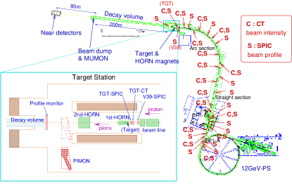
Figure 1: A schematic view of the KEK-PS and neutrino beam line and the location of beam line components. The EP1 neutrino beam line leads protons through a distance of 400 m from the EP1-A extraction point to the target station via the straight and arc sections. The characters “C” and “S” in the figure show the locations of the CT and SPIC installations, respectively. The lower-left inset is a magnified view of the target station. The production target and a set of horn magnets are located in the target station. A pion monitor was installed on two occasions downstream the horn magnets.

II.1.1 Primary proton beam

Protons are accelerated by the KEK-PS to a kinetic energy of 12 GeV. After acceleration, all protons are extracted in a single turn to the neutrino beam line. The duration of an extraction, or a “spill”, is 1.1 $\mu$sec, which contains 9 bunches of protons with a 125 ns time interval between them. As shown in Fig. 1, the beam is extracted toward the north, bent by 90^∘ toward the direction of SK, and transported to the target station. There is a final steering magnet just before the target which directs the beam to SK at an angle of about 1^∘ downward from horizontal.

The beam intensity is monitored by 13 current transformers (CTs) installed along the neutrino beam line as shown in Fig. 1. The CTs are used to monitor the beam transportation efficiency. The overall transportation efficiency along the beam line is about 85%. A CT placed just in front of the production target is used to estimate the total number of protons delivered to the target. A typical beam intensity just before the target is about $5\times 10^{12}$ protons in a spill.

In order to measure the profile and the position of the beam, 28 segmented plate ionization chambers (SPICs) are also installed (Fig. 1). They are used to steer and monitor the beam, while the last two SPICs in front of the target are used to estimate the beam size and divergence, which is used as an input to our beam Monte Carlo (MC) simulation.

II.1.2 Hadron production target and horn magnets

A hadron production target and a set of horn magnets are placed in the target station. Protons hit the target and a number of secondary particles are generated at the production target. Two toroidal magnetic horns are employed to focus positively charged particles, mainly $\pi^{+}$’s, in the forward direction by the magnetic field. A typical focusing of transverse momentum by the horn magnets is about 100 MeV/$c$ per meter. The momenta of focused pions are around 2$-$3 GeV/$c$, which corresponds to about 1.0$-$1.5 GeV of energy for those neutrinos decaying in the forward direction. According to our Monte Carlo simulation, the flux of neutrinos above 0.5 GeV is 22 times greater with horn magnets with 250 kA current than without the horn current.

A schematic view of the horn magnets is shown in Fig. 2. The dimensions of the first horn are 0.70 m in diameter and 2.37 m in length, while those of the second horn are 1.65 m in diameter and 2.76 m in length. Both horns are cylindrically symmetric in shape. The production target, a rod of a length of 66 cm and diameter of 3 cm, made of aluminum alloy 6061-T, is embedded inside the first horn. The target diameter was 2 cm in June 1999 and was changed to 3 cm in November 1999 for improved mechanical strength. The target also plays the role of inner conductor of the first horn, making a strong magnetic field inside the horn to achieve high focusing efficiency. The second horn is located 10.5 m downstream from the first horn, playing the role of a reflector, which re-focuses over-bent low energy pions, and in addition further focuses under-bent high energy pions.

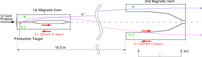
Figure 2: Schematic view of the two horn magnets. An electrical current of 250 kA is supplied to both horns, creating a toroidal magnetic field inside the horns. The production target, an aluminum rod of 66 cm in length and 3 cm in diameter, is embedded inside the first horn magnet, which also plays the role of inner conductor of the horn. The second horn is located 10.5 m downstream of the first horn.

Pulsed current with a duration of 2 msec and an amplitude of 250 kA (200 kA in June 1999) is supplied by four current feeders to each horn. The peaking time of the current is adjusted to match the beam timing. The maximum magnetic field in the horn is 33 kG at the surface of the target rod with 3 cm diameter target and 250 kA horn current.

The values of the current supplied to the horn magnets are read out by CTs put in between current feeders and recorded by a flash analog-to-digital converter (FADC) on a spill-by-spill basis. Overall current and current balance between feeders are monitored to select good beam spills. The magnetic field inside the prototype of the first horn was measured using pickup coils; results showed that the radial distribution of the field was in agreement with the design distribution and the azimuthal symmetry was confirmed to within a measurement error of 15%. Detailed descriptions of the horn magnets are found in Yamanoi et al. (1997, 1999); Kohama (1997).

A pion monitor (PIMON) was installed on two occasions just downstream of the horn magnets, as shown in Fig. 1, in order to measure the momentum and angular distributions of pions coming through the horn magnets. The PIMON will be described in detail later in Sec. V.

II.1.3 Decay volume, beam dump, and muon monitors

The positive pions focused by the horn magnets go into a 200 m long decay volume which starts 19 m downstream of the production target, where the $\pi^{+}$ decay: $\pi^{+}\to\mu^{+}\,\nu_{\mu}$. The decay volume is cylindrical in shape and is separated into three sections with different dimensions. The diameters of the pipe are 1.5 m, 2 m, and 3 m in the first 10 m, the following 90 m, and the remaining 100 m sections, respectively. The decay volume is filled with helium gas of 1 atm (rather than air) to reduce the loss of pions by absorption and to avoid uncontrollable pion production in the gas. The beam dump is located at the end of the decay volume to absorb all the particles except for neutrinos. It consists of 3.5 m thick iron, 2 m thick concrete, and a region of soil about 60 m long.

There is a pit called the “muon-pit” just downstream of the iron and concrete shields. Muons with momentum greater than 5.5 GeV/$c$ can reach the muon-pit. The flux at the pit is roughly $10^{4}~{}\mathrm{muons/cm^{2}/spill}$. The parent particles of both muons and neutrinos are pions, so the profile center of muons corresponds to that of neutrinos. A change in the beam direction by 3 mrad corresponds to a change in the neutrino flux and spectrum at SK of about 1%, and hence it must be controlled and monitored to be within 3 mrad. Fig. 3 shows a schematic view inside the pit. Two detectors (MUMONs) are installed in it: one is an ionization chamber (ICH) and the other is an array of silicon pad detectors (SPD). The purpose of these detectors is to measure the profile and intensity of muons penetrating the shields on spill-by-spill basis.

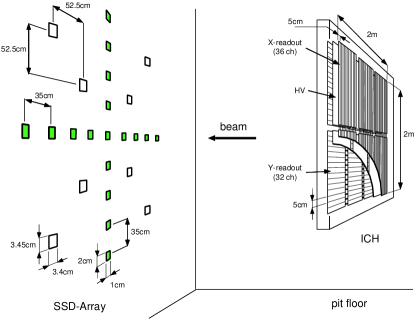
Figure 3: A schematic view inside the muon-pit. An ionization chamber (ICH) and an array of silicon pad detectors (SPD) are located inside the muon-pit.

An ICH is a segmented plate chamber with a size of 190 cm (horizontal) $\times$ 175 cm (vertical). It consists of six modules of size 60 cm $\times$ 90 cm, 3 modules in the horizontal direction and 2 modules in the vertical direction. The gap between modules is 25 cm in horizontal and 15 cm in vertical (Fig. 3). The corresponding strip lines of adjoining modules are electrically connected over the gaps to make long strip lines of length of $\sim$180 cm. There are 36 horizontal readout channels and 32 vertical channels. The channel-to-channel uniformity is calibrated by moving ICH horizontally and vertically Maruyama (2000) assuming stability of the muon beam. The relative gain of the channels has been stable within an accuracy of several percent.

Two types of SPDs are used: one is a small SPD which has a sensitive area of 1 cm $\times$ 2 cm with a depletion layer thickness of 300 $\mu$m, and the other is a large SPD which has a sensitive area of 3.4 cm $\times$ 3.05 cm with a depletion layer thickness of 375 $\mu$m. Seventeen small SPDs are arranged along the horizontal and the vertical axes at 35 cm intervals while nine large SPDs are in diagonal arrays at 74.2 cm intervals. The sensitivity of each small SPD was measured using an LED light source at a test bench and it was found that all the small SPDs agree within 6% Maruyama (2000). The sensitivity difference between the large SPDs was measured using the muon beam at the muon-pit. All the large SPDs were aligned along the beam axis simultaneously and the output charge from each SPD was compared to obtain the relative gain factor. The gain factors have an uncertainty of 10% due to the $z$-dependence of the muon beam intensity Maruyama (2000).

II.2 Summary of beam operation

The construction of neutrino beam line was completed early in 1999 and beam commissioning started in March 1999. The beam line and all the components were constructed and aligned within an accuracy of 0.1 mrad with respect to a nominal beam axis which was determined based on the results of a global positioning system (GPS) survey accurate to 0.01 mrad between KEK and Kamioka sites Noumi et al. (1997). In June 1999, the neutrino beam and detectors were ready to start data-taking for physics. We took data on and off over the period from June 1999 to November 2004, which is divided into five subperiods according to different experimental configurations: June 1999 (Ia), November 1999 to July 2001 (Ib), December 2002 to June 2003 (IIa), October 2003 to February 2004 (IIb), and October 2004 to November 2004 (IIc). The horn current was 200 kA (250 kA) and the diameter of the production target was 2 cm (3 cm) in the Ia (other) period. The SK PMTs were full density for Ia and Ib, but were half density for IIa, IIb and IIc. There was a lead-glass calorimeter (LG) installed in between a scintillating-fiber/water-target tracker (SciFi) and a muon range detector (MRD) during the Ia and Ib periods; it was replaced by a totally active fine-segmented scintillator tracker (SciBar) for IIa, IIb and IIc. Only the first four layers of the SciBar detector were installed for IIa while it was in its full configuration for IIb and IIc. Furthermore, the water target in the SciFi was replaced by aluminum rods during IIc. The different experimental configurations for the different periods are briefly summarized in Table 1.

The number of protons delivered to the target is summarized in Table 1, and shown as a function of time in Fig. 4. Among the delivered spills, spills which satisfy the following criteria are used for the physics analysis: (1) beam spills with normal machine status. Spills during machine studies, beam tuning, and several beam studies are discarded. (2) Beam spills with no trouble in the beam components and data acquisition systems. (3) Beam spills with the proton intensity greater than $1\times 10^{12}$ protons. (4) Beam spills with the horn current greater than 240 kA (190 kA) for the period other than Ia (for the Ia period). The number of protons on target (POT) for the physics analysis is summarized in Table 1 as well as the total number of protons delivered. In total, $1.049\times 10^{20}$ protons were delivered to the production target while $0.922\times 10^{20}$ POT are used in our physics analysis.

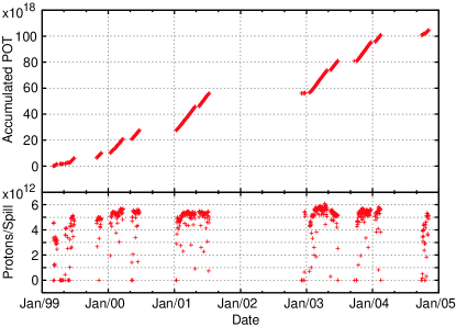
Figure 4: The number of protons delivered to the production target in the period from March 1999 to November 2004. The horizontal axis corresponds to the date. The upper figure shows the total number of protons on target (POT) accumulated since March 1999, and the lower figure shows the POT per spill averaged in a day. In total, $104.90\times 10^{18}$ protons were delivered during the entire period including beam commissioning and tuning periods.

Table 1: Summary of the number of protons on target and the experimental configuration for each running period. The row labeled “LG/SciBar configuration” indicates the detector installed between the SciFi and MRD detectors. For the row “SK configuration”, “SK-I” refers to the configuration with full PMT density while “SK-II” refers to that with half density. See the text for more detailed description of the experimental configurations. The delivered POT shown in the table includes the beam delivered during commissioning and beam tuning work before the physics runs.

Periods	Ia	Ib	IIa	IIb	IIc	total
	Jun.’99	Nov.’99$-$Jul.’01	Dec.’02$-$Jun.’03	Oct.’03$-$Feb.’04	Oct.’04$-$Nov.’04
Delivered POT $(\times 10^{18})$	6.21	49.85	24.91	20.15	3.78	104.90
POT for analysis $(\times 10^{18})$	3.10	44.83	22.57	18.61	3.12	92.23
Horn current	200 kA	250 kA	250 kA	250 kA	250 kA
Target diameter	2 cm	3 cm	3 cm	3 cm	3 cm
SK configuration	SK-I	SK-I	SK-II	SK-II	SK-II
LG/SciBar configuration	LG	LG	SciBar (4 layers)	SciBar	SciBar
Target material in SciFi	water	water	water	water	aluminum

During these periods, the direction of the neutrino beam was monitored by MUMON in the muon-pit. Fig. 5 shows the stability of the center of the muon profile measured by the ionization chamber (ICH) in MUMON. The beam was pointed to the direction of SK within $\pm 1~{}{\rm mrad}$ during the whole run period, so that the neutrino flux and spectrum at SK was stable within much better than 1%.

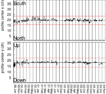
Figure 5: Stability of the center of muon profile measured by the ionization chamber (ICH) in MUMON. The upper figure shows the profile center of the horizontal direction and the lower figure shows that of the vertical direction. In each figure, the beam direction to SK measured by GPS and $\pm 1~{}{\rm mrad}$ off the center are indicated by horizontal lines. The data shown here are after good beam selection.

II.3 K2K neutrino beam simulation

We use a neutrino beam Monte Carlo (beam MC) simulation program to study our neutrino beam properties. The beam line geometry is implemented in GEANT Brun et al. (1987) and particles are tracked in materials until they decay into neutrinos or are absorbed in the material. The tracks of neutrinos are extrapolated along a straight line to the near detector (ND) and Super-Kamiokande (SK) and the fluxes and the energy spectrum at these locations are determined.

In the simulation program, protons with a kinetic energy of 12 GeV are injected into the aluminum production target. The profile and divergence are assumed to be Gaussian-like and the values measured by two SPICs in front of the target are used as inputs. An empirical formula for the differential cross-section by J. R. Sanford and C. L. Wang Sanford and Wang (1967); Wang (1970) is used to simulate the primary hadron production in the target. The Sanford-Wang formula is expressed as following:

$$\displaystyle{\frac{d^{2}\sigma}{d\Omega dp}} = C_{1}\,p^{C_{2}}\left(1-\displaystyle{\frac{p}{p_{B}}}\right)\,\times$$

$$\exp\!\left(-\displaystyle{\frac{C_{3}\,p^{C_{4}}}{p_{B}^{C_{5}}}}-C_{6}\,\theta\,(p-C_{7}\,p_{B}\,\cos^{C_{8}}\!\theta)\right)\,,$$

where ${d^{2}\sigma}/{d\Omega dp}$ is the double differential cross section of particle production per interacting proton in the unit of ${\rm mb}~{}{\rm sr}^{-1}~{}({\rm GeV}/c)^{-1}$, $\theta$ is the angle between the secondary particle and the beam axis in the laboratory frame, $p$ and $p_{B}$ are the momenta of the secondary particle and the incident proton, respectively. The $C_{i}$’s are parameters fitted to existing hadron production data. For the production of positively charged pions, we use as a reference model the $C_{i}$’s obtained from a fit designated the “Cho-CERN compilation”, in which the data used in the compilation mainly come from the measurement of proton-beryllium interactions performed by Cho et al. Cho et al. (1971). The values for $C_{i}$’s are shown in Table 2.

Table 2: The fitted parameters, $C_{i}$’s, in the Sanford-Wang formula for the production of positively charged pions in the Cho-CERN compilation and for the HARP results Catanesi et al. (2006). The target nucleus is beryllium in Cho-CERN compilation while it is aluminum in the HARP results. The values in the table are before the nuclear scaling is applied.

		$C_{1}$	$C_{2}$	$C_{3}$	$C_{4}$	$C_{5}$	$C_{6}$	$C_{7}$	$C_{8}$
HARP		440	0.85	5.1	1.78	1.78	4.43	0.14	35.7
Cho-CERN		238	1.01	2.26	2.45	2.12	5.66	0.14	27.3

A nuclear rescaling is then applied to convert the pion production cross section on beryllium to that on aluminum. The scaling factor, $w$, is defined as

$$w\equiv\left(\frac{A_{\rm Al}}{A_{\rm Be}}\right)^{\alpha(x_{F})}\,,$$ (4)

where $A_{\rm Al}$ and $A_{\rm Be}$ are atomic masses for aluminum and beryllium, respectively, and an index $\alpha(x_{F})$ is expressed as

$$\alpha(x_{F})=0.74+x_{F}(-0.55+0.26x_{F})$$ (5)

as a function of the Feynman $x$ variable, $x_{F}$.

Negatively charged pions and charged and neutral kaons are generated as well as positively charged pions using the same Sanford-Wang formula with different sets of $C_{i}$’s. For negative pion production, the parameters in Cho et al. (1971) are used, while those described in Yamamoto (1981) are used for the kaon production.

Generated secondary particles are tracked by GEANT with the GCALOR/FLUKA Gabriel et al. (1977); Zeitnitz and Gabriel (1994); Fasso et al. (1993) hadron model through the two horn magnets and the decay volume until they decay into neutrinos or are absorbed in materials.

Since GEANT treats different types of neutrinos identically, we use a custom-made simulation program to treat properly the type of neutrinos emitted by particle decays. Charged pions are treated so that they decay into muon and neutrino ($\pi^{+}\to\mu^{+}\,\nu_{\mu},\pi^{-}\to\mu^{-}\,\overline{\nu}_{\mu}$, called $\pi^{\pm}_{\mu 2}$) with branching fraction of 100%. The kaon decays considered in our simulation are so-called $K^{\pm}_{\mu 2}$, $K^{\pm,0}_{e3}$ and $K^{\pm,0}_{\mu 3}$ decays. Their branching ratios are taken from the Particle Data Group Eidelman et al. (2004). Other decays are ignored. Neutrinos from $K^{0}_{S}$ are ignored since the branching ratio for $K^{0}_{S}$ decaying to neutrinos is quite small. The Dalitz plot density of $V$$-$$A$ theory Eidelman et al. (2004); Commins and Bucksbaum (1983) is employed properly in $K_{\ell 3}$ decays. Muons are considered to decay via $\mu^{\pm}\to e^{\pm}\,\,\,\nu_{e}(\overline{\nu}_{e})\,\,\,\overline{\nu}_{\mu}(\nu_{\mu})$, called $\mu^{\pm}_{e3}$, with 100% branching fraction. The energy and angular distributions of the muon antineutrino (neutrino) and the electron neutrino (antineutrino) emitted from a positive (negative) muon are calculated according to Michel spectra of $V$$-$$A$ theory Commins and Bucksbaum (1983), where the polarization of the muon is taken into account.

The produced neutrinos are extrapolated to the ND and SK according to a straight line and the energy and position of the neutrinos entering the ND and SK are recorded and used in our later simulations for neutrino interaction and detector simulators.

The composition of the neutrino beam is dominated by muon neutrinos since the horn magnets mainly focus the positive pions. Figure 6 shows the energy spectra of each type of neutrino at ND and SK estimated by the beam MC simulation. About 97.3% (97.9%) of neutrinos at ND (SK) are muon neutrinos decayed from positive pions, and the beam is contaminated with a small fraction of neutrinos other than muon neutrinos; $\nu_{e}/\nu_{\mu}\sim 0.013~{}(0.009)$, $\overline{\nu}_{\mu}/\nu_{\mu}\sim 0.015~{}(0.012)$, and $\overline{\nu}_{e}/\nu_{\mu}\sim 1.8\times 10^{-4}~{}(2.2\times 10^{-4})$ at ND (SK).

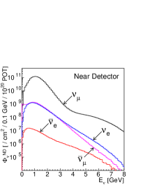
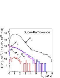
Figure 6: The energy spectrum for each type of neutrino at ND (left) and SK (right) estimated by the beam MC simulation. The neutrino beam is 97.3% (97.9%) pure muon neutrino with contaminations of $\nu_{e}/\nu_{\mu}\sim 0.013~{}(0.009)$, $\overline{\nu}_{\mu}/\nu_{\mu}\sim 0.015~{}(0.012)$, and $\overline{\nu}_{e}/\nu_{\mu}\sim 1.8\times 10^{-4}~{}(2.2\times 10^{-4})$ at ND (SK).

The validity of our beam MC simulation has been confirmed by both the HARP experiment and PIMON measurements, which will be described in detail in Sec. V.

III Neutrino detectors

A near neutrino detector system (ND) is located 300 m downstream from the proton target. The primary purpose of the ND is to measure the direction, flux, and the energy spectrum of neutrinos at KEK before they oscillate. The schematic view of the ND during the K2K-IIb period is shown in Fig. 7.

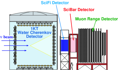
Figure 7: The schematic view of the near neutrino detectors for K2K-IIb period. In K2K-I, the Lead-Glass calorimeter was located at the position of the SciBar detector.

The ND is comprised of two detector systems; a one kiloton water Cherenkov detector (1KT) and a fine-grained detector (FGD) system. The FGD consists of a scintillating-fiber/water-target tracker (SciFi), a Lead-Glass calorimeter (LG) in K2K-I period, a totally active fine-segmented scintillator tracker (SciBar) in K2K-IIb and K2K-IIc periods, and a muon range detector (MRD). The far detector is the 50 kiloton water Cherenkov detector, Super-Kamiokande (SK), which is located 250 km away from KEK and 1000 m (2700 m water equivalent) below the peak of Mt. Ikeno-yama in Gifu prefecture.

III.1 1 kiloton water Cherenkov detector

A one kiloton water Cherenkov detector (1KT) is located in the experimental hall at KEK as the upstream detector. The 1KT detector is a miniature version of SK, and uses the same neutrino interaction target material and instrumentation. The primary role of the 1KT detector is to measure the $\nu_{\mu}$ interaction rate and the $\nu_{\mu}$ energy spectrum. The 1KT detector also provides a high statistics measurement of neutrino-water interactions.

The cylindrical tank, 10.8 m in diameter and 10.8 m in height, holds approximately 1000 tons of pure water. The center of the water tank is 294 m downstream of the pion production target. The water tank is optically separated into the inner detector (ID) and the outer detector (OD) by opaque black sheets and reflective Tyvek^® (a material manufactured by DuPont) sheets. The ID of the 1KT detector is a cylinder of 8.6 m in diameter and 8.6 m in height. This volume is viewed by 680 photomultiplier tubes (PMTs) of 50 cm diameter facing inward to detect Cherenkov light from neutrino events. The PMTs and their arrangement are identical to those of SK; 70 cm spacing between PMTs gives a 40% photocathode coverage. The fiducial volume used for selecting neutrino events in the 1KT is defined as a 25 ton cylindrical region with a diameter of 4 m and a length of 2 m oriented along the beam axis. The OD covers the upstream third of the barrel wall and the whole of the bottom wall. The OD volume is viewed by 68 PMTs of 20 cm diameter, facing outward to veto the incoming particles. The OD is also used to trigger through-going/stopping cosmic ray muon events for detector calibrations.

To compensate for the geomagnetic field which affects the PMT response, nine horizontal Helmholtz coils and seven vertical Helmholtz coils are arranged surrounding the water tank. The water purification system for the 1KT detector circulates about 20 tons/hour of water. The electrical resistance ($\sim$10 M$\Omega$/cm) and water temperature ($\sim$11 ${}^{o}C$) are kept constant by the system.

The 1KT detector data acquisition (DAQ) system is similar to that of SK. The signal from each PMT is processed using custom electronics modules called ATMs, which were developed for the SK experiment and are used to record digitized charge and timing information for each PMT hit over a threshold of about $1/4$ photoelectrons. The DAQ trigger threshold is about 40 PMT hits within a 200 nsec time window in a 1.2 $\mu$sec beam spill gate, where the beam spill gate is issued to all near detectors, synchronized with the beam timing, by the accelerator. The 40 hit threshold is roughly equivalent to the signal of a 6 MeV electron. The pulse shape of the analog sum of all 680 PMTs’ signals (PMTSUM) is also recorded for every beam spill by a 500 MHz flash analog to digital converter (FADC) which enables us to identify multiple interactions in a spill gate. We determine the number of interactions in each spill by counting the peaks in PMTSUM greater than a threshold equivalent to a 100 MeV electron signal.

The physical parameters of an event in the 1KT detector such as the vertex position, the number of Cherenkov rings, particle types and momenta are determined using the same algorithms as in SK Ashie et al. (2005). First, the vertex position of an event is determined from the PMT timing information. With knowledge of the vertex position, the number of Cherenkov rings and their directions are determined by a maximum-likelihood procedure. Each ring is then classified as $e$-like, representing a showering particle ($e^{\pm}$, $\gamma$), or $\mu$-like, representing a non-showering particle ($\mu^{\pm}$, $\pi^{\pm}$), using its ring pattern and Cherenkov opening angle. On the basis of this particle type information, the vertex position of a single-ring event is further refined. The momentum corresponding to each ring is determined from the Cherenkov light intensity. Fully contained (FC) neutrino events, which deposit all of their Cherenkov light inside the inner detector, are selected by requiring the maximum number of photoelectrons on a single PMT at the exit direction of the most energetic particle to be less than 200. The events with the maximum number of photoelectrons greater than 200 are identified as a partially contained (PC) event. This criterion is used because a muon passing through the wall produces a lot of light in the nearest PMTs.

The reconstruction quality, especially the vertex position and angular resolution, are estimated with a MC simulation. The vertex resolution is estimated to be 14.7 cm for FC single-ring events and 12.5 cm for PC single-ring events, while those for multi-ring FC and PC events are 39.2 cm and 34.2 cm, respectively. The angular resolution for single-ring CC-QE events is estimated to be 1.05^∘ for FC events and 0.84^∘ for PC events. As for the capability of the particle identification, 0.3% of muon neutrino CC quasi-elastic events with a single ring are misidentified as $e$-like while 3.3% of electron neutrino CC quasi-elastic events with a single ring are misidentified as $\mu$-like. The momentum resolution for muons is estimated to be 2.0-2.5% in the whole momentum range of the 1KT.

The gain and timing of each PMT are calibrated using a Xe lamp and a N₂ laser as light sources, respectively. The absorption and scattering coefficients of water are measured using laser calibration, and the coefficients in the detector simulation are further tuned to reproduce the observed charge patterns of cosmic ray muon events. The energy scale is calibrated and checked by cosmic ray muons with their decay electrons and neutral current $\pi^{0}$s produced by the K2K neutrino beam. The absolute energy scale uncertainty is ${}^{+3}_{-4}$% while the vertical/horizontal detector asymmetry of the energy scale is 1.7%. The energy scale is stable within about 1% from 2000 to 2004.

The performance of vertex reconstruction is experimentally studied by special cosmic ray muon data utilizing a PVC pipe with scintillating strips at each end inserted vertically into the tank. Cosmic ray muons going through the pipe emulate the neutrino-induced muons whose vertex position is defined at the bottom end of the pipe. This study demonstrates that the vertex reconstruction works as well as we expected from the Monte Carlo simulation. We find a vertex bias difference between data and MC simulation of less than 4 cm for both FC and PC events.

III.2 Scintillating Fiber detector

The scintillating fiber (SciFi) detector is a 6 ton tracking detector with integral water target layers. Details of the design and performance of the detector are described in Refs.Suzuki et al. (2000); Kim et al. (2003). The SciFi detector is used to measure the neutrino spectrum, and to reconstruct with high resolution the charged particle tracks produced in neutrino interactions. It can estimate the rates for quasi-elastic and inelastic interactions and is sensitive to higher energy events, and hence has complementary capabilities to the 1KT detector. The SciFi detector has been in stable operation since 1999 when the first K2K neutrino beam was delivered.

The SciFi detector consists of 20 layers of 2.6 m $\times$ 2.6 m tracking modules, placed 9 cm apart. Each layer contains a double layer of sheets of scintillating fibers arranged, one each, in the horizontal and vertical directions; each sheet is itself two fibers thick. The diameter of each fiber is 0.692 mm. In between the fiber modules, there are 19 layers of water target contained in extruded aluminum tanks. The water level was monitored; it has stayed constant within 1% throughout the experiment, except for a few tanks which drained following an earthquake. This monitoring, as well as measurements when the tanks were filled and later drained, give a fiducial mass of 5590 kg with 1% accuracy. The fiducial mass fractions are 0.700 H₂0, 0.218 Al, and 0.082 HC ($\pm$ 0.004).

The fiber sheets are coupled to an image intensifier tube (IIT) with a CCD readout system. The relative position between the fibers and the CCD coordinate system is monitored periodically by illuminating every 10th or 20th fiber with an electro-luminescent plate placed at the edge of each fiber sheet. In addition, cosmic-rays were used to monitor the gain of the system on a weekly basis.

Hit fibers are extracted using the CCD images. The raw data consists of hit CCD pixels and their digitized brightness. Neighboring hit pixels are grouped to make a pixel cluster. Those clusters are then combined and matched to the location of specific scintillating fibers. The efficiency to identify a fiber through which a charged particle passed is estimated using cosmic ray muons to be about 95%, but closer to 90% at angles within 30 degrees of the beam. After hit fibers are reconstructed, tracks with three or more hit layers are reconstructed using conventional fitting techniques. The efficiency to find a track is also estimated using cosmic ray muons, and is $\sim 70\%$ for tracks with length of three layers, $\sim 87\%$ for four layers, and approaches 100% for longer tracks.

Surrounding the SciFi are two plastic scintillator hodoscope systems. One is placed downstream of SciFi and gives track timing and position information. It also serves as a pre-shower detector for the Lead Glass calorimeter. The other is upstream of SciFi and is used to veto muons and other particles from the beam, primarily from neutrino interactions in the upstream 1KT detector, but also from cosmic rays.

The downstream system consists of 40 scintillator units placed one upon another having a total height of 4 m. Each unit is made of a plastic scintillator 466 cm long, 10.4 cm high, and 4 cm thick. A PMT is attached to each end of the scintillator. The horizontal position of the charged particle can be calculated with 5 cm resolution from the timing information read out by the both end PMT’s. The upstream veto wall is similar, but pairs of scintillators are joined together by optical cement and share a single light guide for each PMT. Thus there are fewer readout channels and the vertical resolution is twice as coarse, but the hodoscope covers the same total area as the one downstream. The charge and timing information from each of the 120 total PMT’s are recorded. The energy deposit measured in the downstream hodoscope is used to select electron neutrino events as described later. The energy resolution of these hodoscopes is estimated using cosmic ray muons to be 7.4% for minimum ionizing particles.

A more detailed description of the hodoscope system can be found in Ahn et al. (2000).

III.3 Scintillating Bar detector

The SciBar detector Nitta et al. (2004) was constructed as an upgrade of the near detector system. The purposes of the SciBar detector are to measure the neutrino energy spectrum and to study the neutrino interaction with high detection efficiency for low momentum particles. The main part of the SciBar detector consists of an array of plastic scintillator strips. Its totally active and finely segmented design allows us to detect all the charged particles produced in a neutrino interaction.

We use extruded scintillator strips produced by FNAL Pla-Dalmau (2001). The dimensions of a strip are 1.3 cm thick, 2.5 cm wide, and 300 cm long. In total, 14,848 scintillator strips are arranged in 64 layers of alternating vertical and horizontal planes. The dimension of the detector is $3\times 3\times 1.7~{}{\rm m^{3}}$ providing the total weight of about 15 tons.

The scintillation light is guided to multi-anode PMTs by wavelength shifting fibers inserted into the holes of scintillator strips. Sixty-four wavelength shifting fibers are bundled together and glued to an attachment to be precisely coupled between fibers and the photo cathode of the multi-anode PMT. Both charge and timing of the PMT outputs are recorded using custom-made electronics Yoshida et al. (2004). The noise level and the timing resolution for minimum-ionizing particle signal are about 0.3 photoelectrons and 1.3 nsec, respectively.

The gain of all multi-anode PMT channels was measured at a test bench prior to the installation. In order to monitor and correct gain drift during operation, the SciBar is equipped with a gain calibration system using LED Hasegawa (2006). The gain stability is monitored with precision better than 1%. Cosmic-ray data are collected between beam spills to calibrate the multi-anode PMT gain and scintillator light yield in-situ. The light yield has been stable within 1 % during operation. The light attenuation length of the wavelength shifting fiber is also measured with cosmic ray muons. It is confirmed to be consistent with the test bench measurement done prior to the installation.

An electromagnetic calorimeter (EC) is installed downstream the tracker part of SciBar to study the amount of the electron neutrino contamination in the beam and $\pi^{0}$ production in neutrino interactions. The calorimeter is made of bars of dimensions $262\times 8\times 4~{}{\rm cm}^{3}$. The bars, a sandwich of lead and scintillating fibers, were originally built for the “spaghetti” calorimeter of the CHORUS neutrino experiment at CERN Buontempo et al. (1994). Each bar is read out by two PMTs per side. In the SciBar-EC, 32 bars are assembled to form a plane of vertical elements, followed by a plane of 30 horizontal bars. The two planes, each 4 cm thick, cover an area of $270\times 262~{}{\rm cm}^{2}$ and $262\times 250~{}{\rm cm}^{2}$, respectively. The EC adds eleven radiation lengths to the tracker part which has about four radiation lengths. The response linearity of the EC is understood to be better than 10%. The energy resolution is about $14\%/\sqrt{E\textrm{[GeV]}}$ as measured with a test beam Buontempo et al. (1994).

To reconstruct neutrino events, hit scintillator strips in SciBar with more than or equal to two photoelectrons (corresponding to about 0.2 MeV) are selected. Charged particles are reconstructed by looking for track projections in each of two dimensional view ($x$-$z$ and $y$-$z$). using a cellular automaton algorithm Glazov et al. (1993). Then, track candidates in two views are combined based on matching of the track edges in $z$ direction and timing information. Reconstructed tracks are required to have hits in more than or equal to three consecutive layers. The minimum length of reconstructible track is, therefore, 8 cm, which is corresponding to 450 MeV/c for protons. The reconstruction efficiency for an isolated track longer than 10 cm is 99%.

III.4 Muon range detector

The muon range detector (MRD) Ishii et al. (2002) has two purposes. One is to monitor the stability of the neutrino beam direction, profile and spectrum by measuring the energy, angle and production point of muons produced by charged-current neutrino interaction by utilizing its huge mass of the iron as the target. The other is to identify the muons produced in the upstream detectors and to measure their energy and angle with combination of other fine grain detectors. This enables us to measure the energy of the incident neutrino.

MRD consists of 12 layers of iron absorber sandwiched in between 13 sets of vertical and horizontal drift-tube layers. The size of a layer is approximately $7.6~{}{\rm m}\times 7.6~{}{\rm m}$. In order to have a good energy resolution for the whole energy region, the upstream four iron plates are 10 cm thick while the downstream eight plates are 20 cm thick. The total iron thickness is 2.00 m covering the muon energy up to 2.8 GeV. MRD has 6,632 drift tubes, each of which is made of aluminum with a cross section of $5~{}{\rm cm}\times 7~{}{\rm cm}$. P10 gas (${\rm Ar}:{\rm CH}_{4}=90\%:10\%$) is supplied to all the tubes. The maximum drift time in a tube is about $1~{}\mu{\rm sec}$. The drift time is digitized by 20 MHz 6-bit TDCs. The total weight of iron is 864 tons and the total mass of MRD including the aluminum drift tubes is 915 tons.

A conventional track finding algorithm is employed to reconstruct tracks from hits. The track finding efficiency is 66%, 95% and 97.5% for tracks with one, two and three traversed iron plate(s), respectively, and it goes up to 99% for longer tracks. The range of track is estimated using the path length of the reconstructed track in iron.

Accurate knowledge of the iron-plate weight is necessary for the measurements of both neutrino interaction rate and track range. Relative thickness of each plate was studied by comparing the event rate using the neutrino beam data. Also, the density was measured directly using a sample of the same iron. Combining these studies, we quote the weight of the iron plates with an accuracy of $1\%$. The relation between the muon energy and the muon range in iron was calculated using a GEANT based Monte Carlo code. There is at maximum $1.7\%$ difference in the muon range among various calculations. We quote the error on energy scale in the range measurement to be $2.7\%$ by linearly adding these two errors.

The energy acceptance and resolutions of the MRD were studied by a Monte Carlo simulation. The acceptance is ranging from 0.3 GeV to 2.8 GeV while the resolution is 0.12 GeV for forward-going muons. The track angular resolution is about 5 degrees and the resolution of the vertex point perpendicular to the beam direction is about 2 cm.

III.5 Lead glass calorimeter

The Lead Glass (LG) calorimeter was located between SciFi and MRD in K2K-I period. The purpose of LG is to distinguish electrons from muons by measuring the energy deposit. The LG calorimeter is made up of 600 cells. A LG cell of approximately $12~{}{\rm cm}\times 12~{}{\rm cm}\times 34~{}{\rm cm}$ is viewed by 3 inch-in-diameter PMT(Hamamatsu, R1652) through a light guide cylinder made also by lead glass. This LG calorimeter was once used in the TOPAZ experiment Kawabata et al. (1988) and reused for the K2K experiment.

The LG detector system reads out only the charge information for each cell. The absolute energy scale of 9 standard LG cells out of 600 were calibrated prior to installation by using an electron beam from the electron synchrotron with the energy range from 50 MeV to 1.1 GeV. The resolution was estimated by this pre-calibration to be 10% at 1 GeV. Position dependence for the energy resolution were also measured to be 4%. The other LG cells were relatively calibrated to the standard cells by cosmic-ray muons.

Responses for muons were also calibrated by using cosmic-ray muons at KEK prior to installation. The relative peak pulse height for PMTs was adjusted to each other within 2%. The responses for charged pions were checked at different momenta (0.3$-$2.0 GeV/$c$) by using the KEK test beam, confirmed to be in good agreement with the expectation by an MC simulation.

III.6 Super-Kamiokande

The far detector of the K2K experiment is Super-Kamiokande, which is located in the Kamioka Observatory, operated by the Institute for Cosmic Ray Research, University of Tokyo. The SK detector is a cylindrically shaped water Cherenkov detector which is 41 m in height, 39 m in diameter and has a total mass of 50 kilotons of water. The water tank is optically separated into a cylindrically-shaped inner detector (ID) and outer detector (OD) by opaque black sheets and Tyvek^® sheets attached to a supporting structure. The ID is viewed by 11,146 20-inch PMTs facing inward covering 40% of the ID surface from June 1999 to 2001 (called SK-I and K2K-I), while it is viewed by 5,182 PMTs enclosed in a fiber reinforced plastic and sealed with acrylic covers on their front surface, covering 19% of the ID surface from December 2002 (SK-II and K2K-II). The transparency and the reflection of these covers in water are 97% and 1%, respectively. In the OD region, outward-facing 1,885 8-inch PMTs are attached to the outer side of the supporting structure. The performance of OD PMTs is improved in SK-II. The fiducial volume is defined to be a cylinder whose surface is 2 m away from the ID wall providing a fiducial mass of 22.5 kilotons. Details of the detector performance and systematic uncertainties in SK-I are written in Fukuda et al. (2003); Ashie et al. (2005). For SK-II, these quantities are estimated using similar methods as used in SK-I. Momentum resolution for SK-II is slightly worse than SK-I; 2.4% and 3.6% for 1 GeV/$c$ muons in SK-I and SK-II, respectively. This is because the number of ID PMTs in SK-II is about a half of SK-I. However, the performance of the vertex reconstruction, the ring counting, and the particle identification in SK-II are almost the same as in SK-I. The purity of the QE interaction in 1-ring $\mu$-like events is 58%. The uncertainty in the energy scale is estimated to be 2.0% for SK-I and 2.1% for SK-II.

In this long baseline experiment, timing information is used to distinguish between beam neutrino events and cosmic ray induced background events in the SK detector. The GPS is used to synchronize the timing of the beam spill between KEK and SK. At both sites are a free running 50 MHz (32-bit) local time counter connected to a GPS receiver and an event trigger (at Super-K) or the beam spill trigger (at KEK). At first, a quartz oscillator was used with good results, and later oscillator drift was improved further with a rubidium clock. This counter is synchronized using the one pulse-per-second signal from the GPS. In this way, events can be synchronized within approximately 50 ns, after compensating for oscillator drift. This is confirmed by comparing a second, independent timing system at each site which gives the same result as the primary system within 35 ns 99% of the time. As described later in this paper, this accuracy is sufficient to observe the neutrino beam’s bunch structure in the SK neutrino data. The system is described more completely in Berns and Wilkes (2000).

IV Neutrino interaction simulation

The neutrino interaction simulation plays an important role both in estimating the expected number of neutrino interactions and in deriving the energy spectrum of neutrinos from the data. The Monte Carlo program simulates neutrino interactions with protons, oxygen, carbon and iron, which are the target materials of the neutrino detectors.

In the simulation program, we include the following charged and neutral current neutrino interactions: quasi-elastic scattering ($\nu\ N\rightarrow\ell\ N^{\prime}$), single meson production ($\nu\ N\rightarrow\ell\ N^{\prime}\ m$), coherent $\pi$ production ($\nu\ ^{16}{\rm O}(^{12}{\rm C},^{56}{\rm Fe})\ \rightarrow\ \ell\ \pi\ ^{16}{\rm O}(^{12}{\rm C},^{56}{\rm Fe})$), and deep inelastic scattering ($\nu N\ \rightarrow\ell\ N^{\prime}\ hadrons$). In these reactions, $N$ and $N^{\prime}$ are the nucleons (proton or neutron), $\ell$ is the lepton, and $m$ is the meson. For the single meson production processes, the $K$ and $\eta$ are simulated as well as the dominant $\pi$ production processes. If the neutrino interaction occurs in oxygen or other nuclei, the re-interactions of the resulting particles with the remaining nucleons in the nucleus are also simulated.

IV.1 Quasi-elastic scattering

The formalism of quasi-elastic scattering off a free neutron used in the simulation programs is described by Llewellyn-Smith Llewellyn Smith (1972). For scattering off nucleons in the nucleus, we use the relativistic Fermi gas model of Smith and Moniz Smith and Moniz (1972). The nucleons are treated as quasi-free particles and the Fermi motion of nucleons along with the Pauli exclusion principle is taken into account. The momentum distribution of the target nucleon is assumed to be flat up to a fixed Fermi surface momentum of 225 MeV/$c$ for carbon and oxygen and 250MeV/$c$ for iron. The same Fermi momentum distribution is also used for all of the other nuclear interactions. The nuclear potential is set to 27 MeV for carbon and oxygen and 32 MeV for iron.

IV.2 Single meson production

Rein and Sehgal’s model is used to simulate the resonance production of single $\pi$, $K$ and $\eta$ Rein and Sehgal (1981, 1983); Rein (1987). This model divides the interaction into two parts. First there is the interaction

$$\nu+N\rightarrow\ell+N^{*},$$

which is then followed by

$$N^{*}\rightarrow\pi(\rm{\ or\ }K\rm{\ or\ }\eta)+N^{\prime},$$

where $N$ and $N^{\prime}$ are the nucleons, and $N^{*}$ is the baryon resonance like $\Delta(1232)$. The mass of the intermediate resonance is restricted to be less than 2 GeV/$c^{2}$. To determine the direction of the pion in the final state, we also use Rein and Sehgal’s method for the dominant resonance $P_{33}$(1232). For the other resonances, the directional distribution of the generated pion is set to be isotropic in the resonance rest frame. The angular distribution of $\pi^{+}$ has been measured for the $\nu p\rightarrow\mu^{-}p\pi^{+}$ mode Kitagaki et al. (1986) and the results agree well with the Monte Carlo prediction. The Pauli blocking effect in the decay of the baryon resonance is taken into account by requiring that the momentum of the nucleon should be larger than the Fermi surface momentum. In addition, the delta may be absorbed by the nucleus. For these events there is no pion in the final state, and only a lepton and nucleon are emitted Singh et al. (1998). We explicitly make this happen for 20% of the deltas produced. Single $K$ and $\eta$ productions are simulated using the same framework as for single $\pi$ production processes.

Both the quasi-elastic and single-meson production models contain a phenomenological parameter (the axial vector mass, $M_{A}$), that must be determined by experiment. As the value of $M_{A}$ increases, interactions with higher $Q^{2}$ values (and therefore larger scattering angles) are enhanced. The $M_{A}$ parameters in our Monte Carlo simulation program are set to be 1.1 GeV for both the quasi-elastic and single-meson production channels based on the analysis of the near detector data  Ahn et al. (2003).

Coherent single $\pi$ production, the interaction between a neutrino and the entire nucleus, is simulated using the formalism developed by Rein and Sehgal Rein and Sehgal (1983). Here, only the neutral current interactions are considered because the cross-section of the charged current coherent pion production was found to be very small at the K2K beam energy Hasegawa et al. (2005).

IV.3 Deep inelastic scattering

In order to calculate the cross-section for deep inelastic scattering, we use the GRV94 parton distribution functionsGluck et al. (1995). Additionally, we have included the corrections in the small $q^{2}$ region developed by Bodek and Yang Bodek and Yang (2002). In the calculation, the hadronic invariant mass, $W$, is required to be larger than 1.3 GeV/$c^{2}$. Also, the multiplicity of pions is restricted to be larger than or equal to two for $1.3<W<2.0~{}{\rm GeV}/c^{2}$, because single pion production is already taken into account as previously described. In order to generate events with multi-hadron final states, two models are used. For $W$ between 1.3 and 2.0 GeV/$c^{2}$, a custom-made program Nakahata et al. (1986) is employed while PYTHIA/JETSET Sjostrand (1994) is used for the events whose $W$ is larger than 2 GeV/$c^{2}$.

The total charged current cross sections including quasi-elastic scattering, single meson production and deep inelastic scattering are shown in Fig. 8 overlaid with data from several experiments.

Figure 8: Charged current total cross section divided by $E_{\nu}$ for neutrino nucleon charged current interactions. The solid line shows the calculated total cross section. The dashed, dot and dash-dotted lines show the calculated quasi-elastic, single-meson and deep-inelastic scatterings, respectively. The data points are taken from the following experiments: ($\triangle$)ANLBarish et al. (1977), ($\bigcirc$)GGM77Bonetti et al. (1977), ($\bullet$)GGM79(a)Ciampolillo et al. (1979),(b)Armenise et al. (1979), ($\ast$)SerpukhovBelikov et al. (1985), ($\Diamond$)ANL82Radecky et al. (1982), ($\star$)BNL86Kitagaki et al. (1986), ($\blacksquare$)CCFR90Auchincloss et al. (1990), ($\blacktriangledown$)CDHSW87Berge et al. (1987), ($\times$)IHEP-JINR96Anikeev et al. (1996), ($+$)IHEP-ITEP79Vovenko et al. (1979), ($\Box$)CCFRR84MacFarlane et al. (1984), and ($\blacktriangle$)BNL82Baker et al. (1982).

IV.4 Nuclear effects

The intra-nuclear interactions of the mesons and nucleons produced in neutrino interactions in the carbon, oxygen or iron nuclei are also important to consider for this analysis. Any absorption or change of kinematics of these particles will affect the event type classification. Therefore, the interactions of $\pi$, $K$, $\eta$ and nucleons are also simulated in our program. These interactions are treated using a cascade model, and each of the particles is traced until it escapes from the nucleus.

Among all the interactions of mesons and nucleons, the interactions of pions are most important, since both the cross sections for pion production for neutrino energies above 1 GeV and also the interaction cross sections of pions in the nucleus are large. In our simulation program, the following pion interactions in nucleus are considered: inelastic scattering, charge exchange and absorption. The actual procedure to simulate these interactions is as follows: first the generated position of the pion in nucleus is set according to the Woods-Saxon nucleon density distribution Woods and Saxon (1954). Then, the interaction mode is determined by using the calculated mean free path of each interaction. To calculate these mean free paths, we adopt the model described by Salcedo et al. Salcedo et al. (1988). The calculated mean free paths depend not only on the momentum of the pion but also on the position of pion in the nucleus.

If inelastic scattering or charge exchange occurs, the direction and momentum of pion are determined by using the results of a phase shift analysis obtained from $\pi-N$ scattering experiments Rowe et al. (1978). When calculating the pion scattering amplitude, the Pauli blocking effect is also taken into account by requiring the nucleon momentum after the interaction to be larger than the Fermi surface momentum at the interaction point.

This pion interaction simulation is tested by comparison with data using the following three interactions: $\pi^{12}$C scattering, $\pi^{16}$O scattering and pion photo-production ($\gamma+^{12}$C $\rightarrow\pi^{-}+X$). The importance of including the proper treatment of nuclear effects is illustrated in Fig. 9 which shows the momentum distribution for neutral current single $\pi^{0}$ production in the water target both with and without having them applied.

Figure 9: The $\pi^{0}$ momentum distributions for neutral current single $\pi$ production processes off the water target and for the K2K neutrino beam at the near detector. The solid and dashed lines show the spectrum without and with the pion nuclear effects.

The re-interactions of the recoil protons and neutrons produced in the neutrino interactions are also important, because the proton tracks are used to select quasi-elastic like events. This is done with the SciFi and SciBar near detectors, and allows us to estimate the neutrino energy. Nucleon-nucleon interactions modify the outgoing nucleon’s momentum and direction, which also affects whether the nucleon will be above detection threshold Walter (2002). Both elastic scattering and pion production are considered. In order to simulate these interactions, a cascade model is again used and the generated particles in the nucleus are tracked using the same code as for the mesons.

V The far/near flux ratio

V.1 Definition of the far-to-near ratio

The effects of neutrino oscillation appear as a reduction in the number of neutrino events and a distortion of the neutrino energy spectrum in SK. The observations for these quantities are compared to their expectations in SK to study neutrino oscillation. The ND measures the neutrino flux and spectrum before neutrinos oscillate. Those measurements are then extrapolated by the expected ratio of muon neutrino fluxes at the far and near detector locations, the far-to-near ($F/N$) flux ratio, to predict the number of neutrino events and energy spectrum in SK.

The neutrino flux at any distance from its source can be predicted when the geometry of the decay volume and the momenta and directions of the pion parents of neutrinos are provided. Due to the finite size of the decay volume and the detectors, the neutrino flux does not simply obey an $L^{-2}$ rule (where $L$ is distance from the neutrino source); rather the flux ratio between far and near detectors has some dependence on neutrino energy. Therefore, we define the $F/N$ flux ratio, $R^{\mathrm{F/N}}$, as

$$R^{\mathrm{F/N}}=\frac{\Phi^{\rm SK}(E_{\nu})}{\Phi^{\rm ND}(E_{\nu})}\,,$$ (6)

where $\Phi^{\rm SK(ND)}(E_{\nu})$ is the neutrino energy spectrum at SK (ND).

The $F/N$ flux ratio is estimated by our beam MC simulation. In this simulation, while we use the Cho-CERN compilation as a reference model, we employ the HARP experiment Catanesi et al. (2006) result as an input for simulation of pion production. The pion production measurement done by HARP is of direct relevance for K2K, since it uses the same beam proton momentum and the same production target, and it covers a large fraction of the phase space contributing to the K2K neutrino flux. The details of the HARP measurements are described in Sec. V.2. The pion monitor (PIMON) measurement is performed for a confirmation of the validity of the beam MC simulation. It gives us in-situ information on the momentum and the direction of pions entering the decay volume after they are focused by the horn magnetic fields although the PIMON is not sensitive to pions below 2 GeV/$c$ (corresponding to neutrinos below 1 GeV) due to its threshold. A description of the PIMON measurement is given in Sec. V.3.

V.2 Prediction of far-to-near ratio from the HARP result

The dominant uncertainty in neutrino flux predictions for conventional neutrino beams is due to the pion production uncertainty in the hadronic interactions of primary beam protons with the nuclear target material. In this analysis, we use the results provided by the HARP experiment at CERN as input to the pion production simulation. The HARP experiment precisely measured the positively-charged pion production in the interactions of 12.9 GeV/$c$ protons in a thin aluminum target Catanesi et al. (2006).

The HARP experiment took data in 2001 and 2002 in the CERN PS T9 beamline, in order to study in a systematic and accurate way hadron production for a variety of produced hadrons (pions and kaons in particular) with large phase space coverage. Data were taken as a function of incident beam particle type (protons, pions), beam momentum (from 1.5 to 15 GeV/$c$), nuclear target material (from hydrogen to lead), and nuclear target thickness (from 2% to more than 100% hadronic interaction length fraction). Secondary tracks are efficiently reconstructed in the HARP forward spectrometer via a set of drift chambers located upstream and downstream with respect to a dipole magnet. Particle identification for forward tracks is obtained with a time-of-flight system, a Cherenkov threshold detector, and an electromagnetic calorimeter.

In particular, the recent HARP pion production measurement Catanesi et al. (2006) is directly relevant for the K2K $F/N$ flux ratio because it is obtained for the same proton beam momentum (12.9 GeV/$c$) and nuclear target material (aluminum) as those used to produce the K2K neutrino beam. Moreover, beam MC simulations show that the forward pion production region measured in HARP, $30<\theta_{\pi}<210$ mrad, $0.75<p_{\pi}<6.5$ GeV/$c$, matches well the pion production phase space responsible for the dominant fraction of the K2K muon neutrino fluxes at both the near and far detector locations.

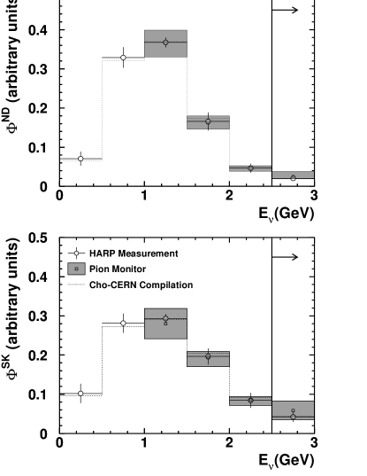
Figure 10: Relatively-normalized muon neutrino flux predictions at the near (top) and far (bottom) detectors. The empty circles with error bars show the central values and shape-only errors based on the HARP $\pi^{+}$ production measurement, the empty squares with shaded error boxes show the central values and errors from the pion monitor (PIMON) measurement, and the dotted histograms show the central values from the Cho-CERN compilation of older (non-HARP) $\pi^{+}$ production data. The PIMON predictions are normalized such that the integrated fluxes above 1 GeV neutrino energy match the HARP ones, at both the near and far detectors.

The result of the pion production measurements described in Catanesi et al. (2006) is incorporated into our beam MC simulation to estimate the neutrino spectra at ND and SK and the energy dependence of the $F/N$ flux ratio in the absence of neutrino oscillations. The relatively-normalized fluxes at ND and SK, $\Phi^{\hbox{\small ND}}$ and $\Phi^{\hbox{\small SK}}$, respectively, predicted by HARP measurement, are shown in Fig. 10, together with the associated total systematic uncertainties, by the empty circles with error bars. Uncertainties in the primary and secondary hadronic interactions, in the pion focusing performance in the horn magnetic fields, and in the primary beam optics, are considered. Here, primary hadronic interactions are defined as hadronic interactions of protons with more than 10 GeV total energy in aluminum, while secondary hadronic interactions are defined to be hadronic interactions that are not primary ones. In the following, the assumptions on systematic uncertainties affecting neutrino flux predictions are summarized.

The uncertainty in the multiplicity and kinematics of $\pi^{+}$ production in primary hadronic interactions is estimated based on the accurate HARP results. In this case, the HARP $\pi^{+}$ Sanford-Wang parameters’ uncertainties and correlations given in Catanesi et al. (2006) are propagated into flux uncertainties using standard error matrix propagation methods: the flux variation in each energy bin is estimated by varying a given Sanford-Wang parameter by a unit standard deviation in the beam MC simulation. An uncertainty of about 30% is assumed for the uncertainty in the proton-aluminum hadronic interaction length. The uncertainty in the overall charged and neutral kaon production normalization is assumed to be 50%.

The systematic uncertainty due to our imperfect knowledge of secondary hadronic interactions, such as $\pi^{+}$ absorption in the target and horns, is also considered. We take the relatively large differences between the GCALOR/GFLUKA Gabriel et al. (1977); Zeitnitz and Gabriel (1994); Fasso et al. (1993) and GHEISHA Fesefeldt (1985) descriptions of secondary interactions, also in comparison to available experimental data, to estimate this uncertainty.

We account for the uncertainties in our knowledge of the magnetic field in the horn system. We assume a 10% uncertainty in the absolute field strength, which is within the experimental uncertainty on the magnetic field strength and the horn current measured using inductive coils during horn testing phase Kohama (1997). Furthermore, a periodic perturbation in azimuth of up to $\pm 15\%$ amplitude with respect to the nominal field strength is assumed as the uncertainty in the field homogeneity, which is also based on the experimental accuracy achieved in the measurement of the magnetic field mapping in azimuth during horn testing Maruyama (2000).

Finally, beam optics uncertainties are estimated based on measurements taken with two segmented plate ionization chambers (SPICs) located upstream of the target. An uncertainty of 1.2 mm and 2.0 mrad in the mean transverse impact point on target and in the mean injection angle, respectively, are assumed based on long-term beam stability studies Inagaki (2001). The uncertainty on the beam profile width at the target and angular divergence is also estimated, based on the $\sim$20% accuracy with which the beam profile widths are measured at the SPIC detector locations Inagaki (2001).

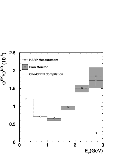
Figure 11: Prediction for the K2K muon neutrino $F/N$ flux ratio in absence of oscillations. The empty circles with error bars show the central values and systematic errors on the muon neutrino flux predictions from the HARP $\pi^{+}$ production measurement discussed in the text, the empty squares with shaded error boxes show the central values and errors from the pion monitor measurement, and the dotted histograms show the central values from the Cho-CERN compilation of older (non-HARP) $\pi^{+}$ production data.

The $F/N$ flux ratio, $\Phi^{\hbox{\small SK}}/\Phi^{\hbox{\small ND}}$, predicted by the HARP $\pi^{+}$ production measurement for primary hadronic interactions with the systematic error evaluation discussed above, in the absence of neutrino oscillations, is shown in Fig. 11 as a function of neutrino energy. We estimate that the flux ratio uncertainty as a function of the neutrino energy binning used in this analysis is at the 2-3% level below 1 GeV neutrino energy, while it is of the order of 4-9% above 1 GeV. We find that the dominant contribution to the uncertainty in $F/N$ comes from the HARP $\pi^{+}$ measurement itself. In particular, the uncertainty in the flux ratio prediction integrated over all neutrino energies is 2.0%, where the contribution of the HARP $\pi^{+}$ production uncertainty is 1.4%. Table 3 shows the contributions of all systematic uncertainty sources discussed above on the far-to-near flux ratio prediction for each neutrino energy bin.

Table 3: Contributions to the uncertainty in the far-to-near flux ratio prediction. The uncertainties are quoted in %. The six columns refer to different bins in neutrino energy, as shown in the table in units of GeV.

Source		0.0$-$0.5	0.5$-$1.0	1.0$-$1.5	1.5$-$2.0	2.0$-$2.5	2.5$-$
Hadron interactions
	Primary interaction rate	0.3	0.9	0.9	2.1	0.2	0.3
	$\pi^{+}$ mult. and kinematics	0.7	2.0	1.8	2.1	2.9	4.7
	Kaon multiplicity	0.1	$<$0.1	0.1	$<$0.1	0.1	4.9
	Secondary interactions	0.3	1.2	2.0	2.1	0.4	0.7
Horn magnetic field
	Field strength	1.1	0.8	1.4	4.2	2.8	3.9
	Field homogeneity	0.3	0.2	0.5	0.3	0.6	0.3
Primary beam optics
	Beam centering	0.1	$<$0.1	$<$0.1	$<$0.1	0.1	0.1
	Beam aiming	0.1	$<$0.1	$<$0.1	0.1	0.4	0.2
	Beam spread	0.1	0.7	1.7	3.4	1.0	3.2
Total		1.4	2.7	3.6	6.5	4.2	8.5

The dotted histograms in Figures 10 and 11 show the central value predicted by using the “Cho-CERN” compilation for primary hadronic interactions, which was used in K2K prior to the availability of HARP data. In this case, the same Sanford-Wang functional form of $\pi^{+}$ production is employed to describe a CERN compilation of $\pi^{+}$ production measurements in proton-beryllium interactions, which is mostly based on Cho et al. data Cho et al. (1971). A nuclear correction to account for the different pion production kinematics in different nuclear target materials is applied. The details of the Cho-CERN compilation are described in Sec. II.3. We find that the predictions of $F/N$ flux ratio by HARP and Cho-CERN are consistent with each other for all neutrino energies. Note that the difference between Cho-CERN and HARP central values represents a difference in hadron production treatment only.

V.3 Confirmation of far-to-near ratio by pion monitor measurement

A confirmation for the validity of the $F/N$ ratio has been performed by in-situ pion monitor (PIMON) measurements. The PIMON was installed on two occasions just downstream the horn magnets to measure the momentum ($p_{\pi}$) versus angle ($\theta_{\pi}$) 2-dimensional distribution of pions entering the decay volume. The PIMON measurements were done twice: once measurement was done in June 1999 for the configuration of Ia period (200 kA horn current with 2 cm target diameter) and the other was done in November 1999 for the configuration of the other periods (250 kA horn current with 3 cm target diameter).

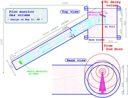
Figure 12: A schematic view of the pion monitor (PIMON). The PIMON consists of a gas vessel, a spherical mirror, and an array of 20 photomultiplier tubes. The gas vessel is filled with freon gas R-318 (${\rm C}_{4}{\rm F}_{8}$). A wedge-shaped spherical mirror is set inside the gas vessel and Cherenkov light produced by the pions in the beam, represented by the concentric circles in the figure, is reflected by the mirror and directed to the array of photo-multiplier tubes which is set in the focal plane.

A schematic view of PIMON is shown in Fig. 12. PIMON is a gas Cherenkov imaging detector which consists of a gas vessel, a spherical mirror, and an array of 20 photomultiplier tubes. The Cherenkov photons emitted by pions passing through the gas vessel are reflected toward and focused onto the PMT array by the spherical mirror. Then, the PMT array on the focal plane detects the Cherenkov image. Due to the characteristics of the spherical mirror, photons propagating in the same direction are focused to the same position on the focal plane, giving us information on the direction of the pions. The pion momentum is also obtained from the size of the Cherenkov ring. Furthermore, a momentum scan can be done by varying the refractive index of the inner gas. Therefore, the momentum and direction of pions can be measured separately by looking at the Cherenkov light distribution on the focal plane.

As shown in Fig. 12, a wedge-shaped mirror is used as the spherical mirror to measure only 1/30 of the beam assuming azimuthal symmetry of the distribution. Its top is aligned to be on the beam center. The reflection angle with respect to beam direction is 30^∘.

An array of 20 PMTs (modified R5600-01Q made by Hamamatsu Corporation) is set 3 m away from the beam center to avoid excess exposure to radiation. The size of the PMT outer socket is 15.5 mm in diameter and the sensitive area of the photocathode is 8 mm in diameter. They are arranged vertically at 35 mm intervals. The array can be moved by a half pitch of the interval along the array, and hence 40 data points (one point for every 1.75 cm) are taken for a Cherenkov light distribution. The relative gain among 20 PMTs was calibrated using Xe lamp before the measurements. The gain ratio between neighboring PMTs was also checked using Cherenkov photons during the run. The error on the relative gain calibration is estimated to be 10% for the June 1999 run and 5% for the November 1999 run. Saturation of the PMTs was observed in the June 1999 run, which was corrected by a second order polynomial function. The uncertainty due to this correction was estimated to be 4% Maruyama (2000).

The gas vessel is filled with freon gas R-318 (${\rm C}_{4}{\rm F}_{8}$). Its refractive index $n$ is varied by changing the gas pressure using the external gas system. The data are taken at several refractive indices ranging between $n=1.00024\!-\!1.00242$ to make PIMON sensitive to different pion momenta. The refractive index was not adjusted beyond $n=1.00242$ since the primary protons also emit Cherenkov photons when $n$ exceeds this value, and become a severe background to the pion measurement. This corresponds to setting a momentum threshold of 2 GeV/$c$ for pions, which corresponds to an energy threshold of 1 GeV for neutrinos. The absolute refractive index is calibrated by the Cherenkov photon distribution from 12 GeV primary protons with the refractive index set at $n=1.00294$.

The Cherenkov light distribution for each refractive index is taken by the PMT array. For the background subtraction, a measurement with the mirror directed away from the direction of PMT array was performed. There is still non-negligible background from electromagnetic showers which mainly come from the decay of neutral pions, $\pi^{0}\to 2\gamma$. The light distribution for this background is estimated using a MC simulation. The normalization in the subtraction is done by using the distribution measured at the lowest refractive index, where the contribution from the electromagnetic components is dominant. After all backgrounds are subtracted, the distribution of the Cherenkov light emitted from pions is obtained as shown in Fig. 13. The prediction of the MC simulation is superimposed as well.

Figure 13: Cherenkov light distributions for various refractive indices measured in November 1999. Dots show data and the histograms show the MC simulation. The refractive indices for each plot are as written in the figure.

A $\chi^{2}$-fitting is employed to extract the $(p_{\pi},\theta_{\pi})$ 2-dimensional distribution from the Cherenkov light distributions with various refractive indices. The $(p_{\pi},\theta_{\pi})$-plane is binned into $5\times 10$ bins; 5 bins in $p_{\pi}$ above 2 GeV/$c$ with 1 GeV/$c$ slice (the last bin is integrated over $p_{\pi}>6$ GeV/$c$) and 10 bins in $\theta_{\pi}$ from $-50$ mrad to $50$ mrad with 10 mrad slices. Templates of the Cherenkov light distributions emitted by pions in these bins are produced for each refractive index using a MC simulation. Then, the weight of the contribution from each $(p_{\pi},\theta_{\pi})$ bin being the fitting parameter, the MC templates are fit to observed Cherenkov light distributions. The fitting is done for the data in June 1999 and in November 1999, separately. The resulting values of fitting parameters and errors on them in November 1999 run are shown in Fig. 14.

Figure 14: The fitting results of pion $(p_{\pi},\theta_{\pi})$ distribution in November 1999 run. The left figure shows the resulting central value of the weighting parameters, and the right figure shows the estimated fitting errors on them (no box means fitting errors are negligibly small.)

The neutrino energy spectra at ND and SK are derived by using the weighting factors obtained above and a MC simulation. The neutrino energy is binned into 6 bins: 0.5 GeV bins up to 2.5 GeV, and integrated above 2.5 GeV. The contribution of pions in each $(p_{\pi},\theta_{\pi})$ bin to neutrino energy bins is estimated by a MC simulation, where to a good approximation it depends only on the pion kinematics and the geometry of the decay volume. Then, the neutrino spectrum is obtained by summing up these contributions weighted by fitted factors. Finally, the ratio of the neutrino spectra at SK to that at ND yields the $F/N$ ratio.

The extracted neutrino spectra and the $F/N$ ratio from the PIMON data taken in November 1999 are shown in Fig. 10 and 11 with empty squares and shaded error boxes. All the systematic uncertainties in deriving them from the PIMON measurement are included in the errors, where the most dominant contributions to the error on the $F/N$ flux ratio come from the fitting error, the uncertainty in the analysis methodology, and the uncertainty in the azimuthal symmetry of the horn magnetic field. Further details on the systematic uncertainties in the PIMON measurement are described in Maruyama (2000).

V.4 The far-to-near ratio in K2K

The $F/N$ flux ratio used to extrapolate the measurements in ND to the expectation in SK is obtained in three independent ways: using the HARP measurement, the Cho-CERN model, and the PIMON measurement, as described in the previous sections. We find that all three predictions of the $F/N$ ratio are consistent with each other within their measurement uncertainties. Among these measurements, we use the one predicted by the HARP measurement in our neutrino oscillation analysis described in this paper, since the HARP pion production measurement was done for the same conditions as K2K experiment: the proton beam momentum and the relevant phase space of pions responsible for the neutrinos in K2K are the same. In particular, the measured momentum region by the HARP experiment reaches below 2 GeV/$c$ down to 0.75 GeV/$c$ where the PIMON is insensitive. The HARP measurement also gives us the most accurate measurements on hadron production.

The central values for the $F/N$ flux ratio as a function of neutrino energy obtained from the HARP $\pi^{+}$ production results, $\overline{R}_{i}$, are given in Tab. 4, where the index $i$ denotes an energy bin number. The total systematic uncertainties on the $F/N$ flux ratio as a function of neutrino energy are given in Tab. 5, together with the uncertainty correlations among different energy bins, expressed in terms of the fractional error matrix $\langle\delta R_{i}\delta R_{j}\rangle/(\overline{R}_{i}\overline{R}_{j})$, where $i,j$ label neutrino energy bins. The $F/N$ central values and its error matrix are used in the analysis for neutrino oscillation described later.

Table 4: Predictions for the $F/N$ muon neutrino flux ratio as a function of neutrino energy, for the HARP model for $\pi^{+}$ production in primary hadronic interactions. The neutrino energy binning is also indicated.

Energy Bin Number $i$	$E_{\nu}$ [GeV]	$\overline{R}_{i}$ $(\times 10^{-6})$
1	0.0$-$0.5	1.204
2	0.5$-$1.0	0.713
3	1.0$-$1.5	0.665
4	1.5$-$2.0	0.988
5	2.0$-$2.5	1.515
6	2.5$-$	1.720

Table 5: Fractional error matrix $\langle\delta R_{i}\delta R_{j}\rangle/(\overline{R}_{i}\overline{R}_{j})$ obtained from the systematic uncertainties on the $F/N$ flux predictions. The neutrino energy binning is the same as in Tab. 4. The values are given in units of $10^{-3}$.

Energy Bin	1	2	3	4	5	6
1	$0.187$	$0.002$	$-0.036$	$-0.372$	$-0.281$	$0.240$
2	$0.002$	$0.728$	$0.868$	$1.329$	$0.698$	$-1.398$
3	$-0.036$	$0.868$	$1.304$	$2.122$	$1.041$	$-2.040$
4	$-0.372$	$1.329$	$2.122$	$4.256$	$2.165$	$-3.799$
5	$-0.281$	$0.698$	$1.041$	$2.165$	$1.779$	$-2.678$
6	$0.240$	$-1.398$	$-2.040$	$-3.799$	$-2.678$	$7.145$

While the neutrino flux predictions given in this section are appropriate for most of the protons on target used in this analysis, a small fraction of the data was taken with a different beam configuration. The K2K-Ia period differed from the later configuration, as described in Sec. II.2. As a result, the far/near flux ratio for June 1999 is separately estimated, in the same manner as described above for later run periods. We find that the flux ratio predictions for the two beam configurations, integrated over all neutrino energies, differ by about 0.4%. The flux ratio prediction for the June 1999 beam configuration and the ND spectrum shape uncertainties are used to estimate the expected number of neutrino events in SK and its error for the June 1999 period.

VI Measurement of neutrino event rate at the near detector

The integrated flux of the neutrino beam folded with the neutrino interaction cross-section is determined by measuring the neutrino event rate at the near site. The event rate at the 1KT detector is used as an input to the neutrino oscillation study. The stability of the neutrino beam is guaranteed by measuring the beam properties by the MRD detector. In addition, the LG and SciBar detectors measure the electron neutrino contamination in the beam to compare to our beam MC simulation.

VI.1 Neutrino event rate

As described in Section III.A, the 1KT water cherenkov detector serves to measure the absolute number of neutrino interactions in the near site and to predict the number of neutrino interactions in the far site. Since the 1KT uses a water target and almost the same hardware and software as SK, the systematic error in the predicted number of interactions at the far site can be reduced. The intensity of the neutrino beam is high enough that multiple neutrino interactions per spill may occur in the 1KT. When this happens it is difficult to reconstruct events. We employ Flash Analog-To-Digital Converters (FADCs) to record the PMTSUM signal (see Section III.A) and we can get the number of neutrino interactions by counting the number of peaks above a threshold. We set this threshold at 1000 photoelectrons (p.e.), approximately equivalent to a 100 MeV electron signal, to reject low energy background such as decay electrons from stopped muons. In Fig. 15, the upper and lower figures show the number of peaks in a spill and the timing information of the peaks, respectively. We can clearly see the 9 micro bunch structure of the beam in the lower figure. The fraction of multi-peak interactions in a spill is about 10% of single-peak spills.

Figure 15: The upper figure shows the number of neutrino interactions in a spill. The lower figure shows the time distribution of peaks of PMTSUM signal which are recorded by FADC. The beam’s 9 micro bunch structure can be seen clearly.

Sometimes the FADCs cannot identify multiple interactions if these events happen in the same bunch and the time gap between the interactions is too small. To correct for this possibility, we employ a MC simulation with multiple interactions to estimate the misidentification probability. The PMTSUM signals recorded by the FADC are simulated, so the same method can be used for the MC simulation and data. We found that the number of interactions in the fiducial volume is underestimated by 2.3% for multiple interactions. The multiple interactions contribute 34% of the total number of interactions, and we have to correct the number of events by this multi-interaction misidentification probability, according to $C_{multi}=1+0.023\times 0.34=1.008$.

The fiducial volume in the 1KT is defined as a horizontal cylinder with axis along the beam direction (z-axis). The radius is 200 cm and the $z$ coordinate is limited to $-200~{}{\rm cm}<z<0~{}{\rm cm}$, where the center of the 1KT ID is defined as $z=0$ cm, and the total fiducial mass is 25 tons. The fiducial volume cut results in an almost pure neutrino sample, rejecting cosmic rays or muons generated by the beam in the materials surrounding the 1KT (beam-induced muons). Figure 16 shows the vertex distributions of data and the MC simulation. Because we simulate only neutrino interactions without beam-induced muons and without the cosmic-ray muons, we can see excess events upstream of the $z$-distribution and the top part of the detector ($y>400~{}{\rm cm}$) in data. The data and the MC simulation are in good agreement in the fiducial volume.

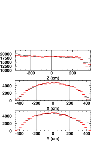
Figure 16: The upper figure shows the vertex distribution in $z$ with an $R_{xy}<200~{}{\rm cm}$ cut. The beam direction is defined as the $z$-axis. Crosses show data, boxes show the MC simulation normalized by area in the fiducial volume, and vertical black lines show the fiducial volume. The middle and lower figures show the $x$ and $y$ distributions, respectively.

Two major background sources are considered. Cosmic ray events usually have a vertex near the upper wall of the inner tank, but some events contaminate the fiducial volume due to failure of the vertex reconstruction. To estimate the background rate, we run the detector without the beam, replacing the spill trigger by a periodical clock signal. The beam-off data are analyzed in the same way as the neutrino data; it is found that cosmic rays in the fiducial volume are 1.0% of the neutrino data. The other important background source is beam-induced muons which can be tagged by PMTs located in the outer detector. After the vertex cut, the remaining events are scanned with a visual event display and the fraction of beam induced muons found is 0.5%. In addition, we had fake events which were produced by signal reflection due to an impedance mismatch of the cables in the 1999 runs only. The total background fraction is estimated to be 1.5% for runs starting in 2000, and 3.1% before 2000.

The neutrino event selection efficiency is calculated based on the MC simulation. The efficiency is defined as:

$$\epsilon^{\mathrm{1KT}}=\frac{\mbox{(\# of reconstructed events in 25t)}}{\mbox{(\# of generated events in 25t)}}$$ (7)

Figure 17 shows the selection efficiency as a function of neutrino energy. The overall efficiency including all energies and all interaction types is 75% for the configuration with a 250kA horn current, and 71% for the 200kA configuration. We had a problem with the FADC in November 1999 which corresponds to 3% of all data, and the efficiency in this period was 5% lower than the other 250kA configuration periods. The dominant inefficiency comes from the single peak selection with a 1000 p.e. threshold by FADC. Figure 18 shows the peak-finding efficiency of the FADC as a function of total charge. The 2000-2004 data plotted in the figure shows that the efficiency curves are stable. The MC event selection efficiency is obtained by smearing the threshold assuming a gaussian distribution, in which the mean and width are obtained by fitting the data.

Figure 17: Neutrino selection efficiency as a function of neutrino energy (GeV).

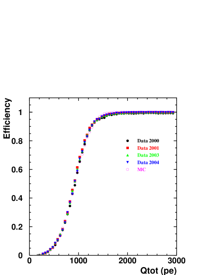
Figure 18: FADC peak finding efficiency is shown as a function of total charge (p.e.). Data taken in 2000, 2001, 2003, and 2004 are shown with the MC simulation.

While the FADC can count the event multiplicity, they do not record information about each PMT channel. The ATM gives the timing and charge information of each individual PMT channel which allows event reconstruction if the spill has a single interaction. Both the FADC and the ATM are required to derive the total number of neutrino interactions:

$$N^{1KT}_{int}=N^{1KT}_{obs}\cdot\frac{N^{total}_{peak}}{N^{single}_{peak}}\cdot\frac{1}{\epsilon^{\mathrm{1KT}}}\cdot\frac{1}{1+R_{BKG}}\cdot C_{multi}$$ (8)

where $N^{1KT}_{int}$ is the total number of neutrino interactions in the 25 t fiducial volume, $N^{1KT}_{obs}$ is the number of events observed in the fiducial volume among single peak events, $N^{total}_{peak}$ is the total number of PMTSUM signal peaks, $N^{single}_{peak}$ is the number of single peak events, $\epsilon^{\mathrm{1KT}}$ is the selection efficiency of neutrino events in the 25t fiducial volume, $R_{BKG}$ is the background fraction, and $C_{multi}$ is the multiple interaction correction.

Table 6 shows the total number of neutrino interactions and the number of protons on target for each period.

Table 6: Number of neutrino interactions in the 1KT.

Period	$POT_{1KT}(10^{18})$	$N^{1KT}_{obs}$	$N^{tot}_{peak}$	$N^{single}_{peak}$	$N^{1KT}_{int}$
Ia	2.6	4282	109119	89782	7206
Ib	39.8	75973	1854781	1475799	130856
IIa	21.6	43538	1061314	832112	73614
IIb	17.1	34258	813599	644723	57308
IIc	2.9	5733	137533	111834	9346

Table 7 shows the systematic uncertainty on the number of neutrino interactions in the 1KT. The dominant error is the uncertainty of the fiducial volume. From the comparison of neutrino interactions in data and the MC simulation, we quantitatively estimate the fiducial volume systematics. Varying the definition of the fiducial volume by about five times the vertex resolution, we observe a difference in the calculated event rate of 1.8%. Most of the difference is due to the $z$-dependence of partially contained events. To estimate this systematic effect, we used deposited energy from neutrino interactions themselves for partially-contained events since the deposited energy is roughly linear in the distance from the vertex to the downstream wall of the ID. We use the “cosmic-ray pipe” muons, described in Section III.1, to define the energy scale for partially-contained events within 2.3%. We do not see evidence for such a bias within the uncertainty of the energy scale. The fiducial uncertainty arising from a vertex bias is therefore 2.3%. We conservatively add those two numbers in quadrature to obtain 3.0% for the uncertainty of the fiducial volume.

The energy scale uncertainty of the 1KT is estimated by using cosmic ray muons which stopped inside of the detector and the reconstructed $\pi^{0}$ mass which mostly comes from neutral current interactions. The absolute energy uncertainty of the 1KT is estimated to be ${}^{+3\%}_{-4\%}$. This energy uncertainty affects $N_{1KT}$ because of the FADC cut. We changed the threshold of the FADC and the effect of energy scale uncertainty is estimated to be 0.3%. The FADC charge is calibrated by the total charge recorded by ATM using single interaction events with a lower threshold (200 p.e.). The stability of the charge scale of FADC is $\pm 5\%$ and its effect on $N_{1KT}$ is $\pm 0.8\%$. $N^{total}_{peak}$ , $N^{single}_{peak}$ and $N^{1KT}_{obs}$ depend on the FADC cut position, but $N^{1KT}_{int}$ should be independent of the cut if the efficiency correction is perfect. We calculate $N^{1KT}_{int}$ changing FADC cut from 200 to 2000 p.e. and confirm the total number of neutrino interaction is stable within $\pm 1.5\%$. In Fig. 19, the upper figure shows the 1KT event rate normalized by muon yields at the SPD in the MUMON (see Section II.A.2). We take 2.0% for the uncertainty of the event rate stability from the root-mean-square (RMS) of the distribution. A comparison between the event rates of the 1KT and the MRD is shown in the lower figure of Fig. 19 as a consistency check. We assign statistical errors as systematic errors for the background and multiple interaction corrections due to the limited numbers of the sample. In total, we quote a $\pm$4.1% error on the number of 1KT neutrino events over the entire K2K run.

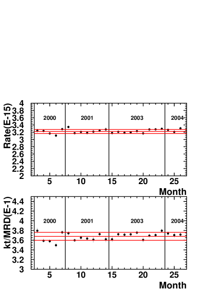
Figure 19: The upper figure shows the event rate in the 1KT normalized by the muon yield of the MUMON. One point corresponds to one month and the 2000 - 2004 data are shown in the figure. The middle line shows the average and the upper and lower lines show the RMS, 1.6%. The lower figure shows the 1KT event rate divided by the MRD event rate, also showing the average and RMS (2.1%).

Table 7: Systematic errors on $N^{1KT}_{int}$.

Source	Error (%)
Fiducial volume	$\pm$ 3.0
Energy scale	$\pm$ 0.3
FADC stability	$\pm$ 0.8
FADC cut position	$\pm$ 1.5
Event rate	$\pm$ 2.0
Background	$\pm$ 0.5
Multi-interaction	$\pm$ 0.7
Total	$\pm$ 4.1

VI.2 Neutrino beam stability

The neutrino beam properties– the profile, beam direction, energy spectrum and event rate– are monitored by the MRD using $\nu_{\mu}$ interactions with iron in order to guarantee stability of the beam for the entire run period.

A neutrino event is identified by a muon track in the MRD with the following selection criteria: only tracks within the time of the beam spill are accepted; tracks with a common vertex and a common timing are taken as a single event with the longest track assumed to be a muon; muons entering or exiting the detector are removed; and muons which traverse one or more iron plates ($N_{layer}\geq 1$) are selected.

The neutrino beam profile is obtained by measuring the vertex distribution in the MRD. The location of the center of the profile gives the beam direction. For this purpose, any muons with reconstructed energy lower than 0.5 GeV or higher than 2.5 GeV are rejected and a cubic fiducial volume of ${\rm 6m}\times{\rm 6m}$ in the upstream 9 iron plates is used, which has a total mass of 419 tons. As shown in Fig. 20, the profile is well reproduced by the MC simulation. The profile center is plotted as a function of time in Fig. 21. The beam direction has been stable throughout the experiment within $\pm$1 mrad from the SK direction. This satisfies the requirement for the direction to be within $\pm$3 mrad, which is described in Section II. The stability of the profile width is also confirmed by the measurement.

The muon energy and angular distributions are also continuously monitored. A cylindrical fiducial volume of radius 3m in the upstream 9 plates is used, where the mass is 329 tons. They show no change as a function of time beyond statistical uncertainty. The muon energy distribution and the angular distribution are plotted monthly in Fig. 22 and Fig. 23, respectively. These results show that the $\nu_{\mu}$ energy spectrum is stable within 2-4% depending on the energy bin. This is well within the spectrum error quoted in the spectrum analysis described in Section VII.

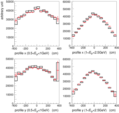
Figure 20: Neutrino beam profiles measured by the MRD. Crosses show the measured profile and the boxes show the Monte Carlo prediction. Normalization is by number of entries. (Top left): horizontal profile for 0.5GeV $<E_{\mu}<$ 1.0GeV. (Top right): horizontal profile for 1.0GeV $<E_{\mu}<$ 2.5GeV. (Bottom left): vertical profile for 0.5GeV $<E_{\mu}<$ 1.0GeV. (Bottom right): vertical profile for 1.0GeV $<E_{\mu}<$ 2.5GeV.

Figure 21: Stability of the neutrino beam direction measured by the MRD. The direction is plotted every five days for the entire experimental period. The solid line shows the SK direction and the dashed lines show $\pm$1 mrad from the center. The direction is required to be stable within $\pm$3mr. The top plot is for the horizontal direction; the bottom for the vertical direction.

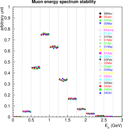
Figure 22: Stability of the muon energy distribution measured by the MRD. Each bin is plotted every month for the entire experimental period except for K2K-Ia. The distributions are normalized by number of entries.

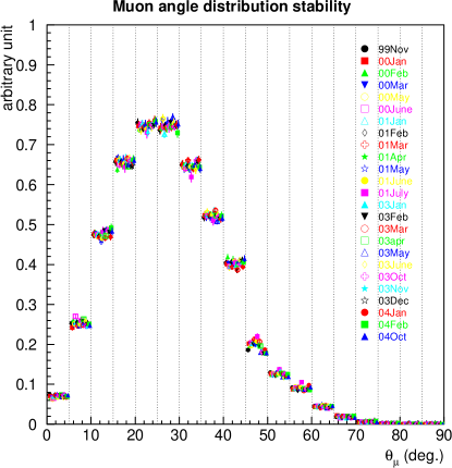
Figure 23: Stability of the muon angular distribution measured by MRD. Each bin is plotted every month for the entire experimental period except for K2K-Ia. The distributions are normalized by their entries.

In order to check the 1KT event rate and to compare the neutrino cross sections in iron and water, the neutrino event rate in the MRD iron is derived. The fiducial mass used is 72.8 tons, which is the 3m-radius cylinder of the upstream three iron plates only. For this purpose, $N_{layer}\geq 2$ is required in order to reduce the hadronic background. The stability of the 1KT event rate divided by the MRD rate is plotted in the bottom figure of Fig. 19.

Since the absolute normalization is less certain, a double ratio of the MRD and 1KT event rates is calculated for the cross-section comparison between iron and water. The result for this double ratio is $({\rm data/MC})_{\rm MRD}/({\rm data/MC})_{\rm 1KT}=1.04\pm 0.003({\rm stat.})^{+0.08}_{-0.11}({\rm sys.})$. The average event rates for MRD and 1KT data for the entire K2K run (except for K2K-Ia) are used. This double ratio should be unity if we correctly understand the iron/water neutrino cross-section ratio in the K2K energy range regardless of the absolute cross section. The sources of the systematic error are summarized in Table 8. Here, the uncertainties due to the neutrino spectrum, NC/CC ratio, and non-QE/QE cross-section ratio have the cancellation between 1KT and MRD taken into account.

Table 8: Systematic errors of the event-rate double ratio $({\rm data/MC})_{\rm MRD}/({\rm data/MC})_{\rm 1KT}$

.

Source		Error +(%)		-(%)
Fiducial volume	+1.6		-5.7
Selection efficiency	+1.2		-5.7
Tracking efficiency	+1.0		-1.0
Beam direction	+1.9		-0.0
MRD detector oriented total		+2.9		-8.1
1KT detector oriented total		+4.1		-4.1
Neutrino spectrum	+0.9		-0.9
NC/CC ratio	+4.0		-3.7
Non-QE/QE ratio	+5.3		-3.7
Spectrum and neutrino int.		+6.7		-5.3
Grand total		+8.4		-10.5

The stability of the detector itself is confirmed as a whole by analyzing the off-spill data which is essentially cosmic-ray data taken between each beam spill. The event rate, angular distributions and $N_{layer}$ distribution are found to be stable.

VI.3 Electron neutrino component

The $\nu_{e}$ component in the beam is measured in the FGD system independently by the LG and by the SciBar detectors. In each detector we perform a search for $\nu_{e}$ interactions by looking for events with an electron in the final state. “Electron” events come essentially only from the $\nu_{e}$ component of the beam, since the ${\nu_{e}}/{\nu_{\mu}}$ flux ratio is about $1.3\times 10^{-2}$, while the ${\overline{\nu}_{e}}/{\nu_{\mu}}$ flux ratio is about $1.8\times 10^{-4}$, and the cross section for $\nu_{\mu}$e scattering is about a factor $1.5\times 10^{-4}$ smaller than that for $\nu_{\mu}$ CC scattering on a nucleon. The measurement of the $\nu_{e}$ events validates the prediction of the ${\nu_{e}}/{\nu_{\mu}}$ flux ratio at the near location obtained from the beam MC simulation. The data-MC comparison also involves the cross-sections of $\nu_{e}$ and $\nu_{\mu}$ interactions, and the measurement is therefore an important check of the MC simulation used to predict the number of $\nu_{e}$ interactions in SK.

The LG measurement Yoshida (2001) is performed by looking for $\nu_{e}$ interactions taking place in the SciFi detector, with the electron detected in the downstream scintillator hodoscope, and its energy measured in the LG calorimeter. Electron events are selected by requiring the following: an interaction vertex inside the SciFi fiducial volume, an energy deposit in the downstream scintillator hodoscope system greater than 20 MeV (2.5 times larger than that expected from a muon), an energy deposit in the LG greater than 1 GeV; and finally, no hit in the MRD matching the electron direction. For an exposure of $2.9\times 10^{19}$ POT, 51 electron candidates are found with an estimated background of 24 $\nu_{\mu}$ induced events. The ${\nu_{e}}/{\nu_{\mu}}$ interaction ratio is estimated to be $1.6\pm 0.4({\rm stat.})^{+0.8}_{-0.6}({\rm syst.})\%$, which is in agreement with the beam MC prediction of 1.3%. The dominant source of the $\nu_{e}$-induced component of CC interactions is muon decay (87%) in the beam, and the remainder comes from kaon decay.

The measurement of the $\nu_{e}$ contamination in the beam has also been performed using the SciBar plus EC detector, with a statistics corresponding to $2.1\times 10^{19}$ POT. The search for electrons is mainly based on the signals from the EC, the electromagnetic calorimeter which follows the tracking section of the SciBar. The two planes of the EC correspond to approximately 5.5 radiation lengths (X₀) each, so that electrons in the 1 GeV energy range are almost fully contained. The average energy lost by a muon or pion traversing one plane is small, of the order of 50 MeV (with $\sim$ 60 MeV full width). Therefore, to look for electrons we select events with a large signal in a restricted region of the first EC plane. We require $E_{1}>350$ MeV, where $E_{1}$ is the energy in a cluster of 20 cm width centered in the module with maximum signal. We also apply conditions on the energy release $E_{2}$ in the 20 cm wide cluster of highest energy of the second plane of the EC. We require ${E_{2}}/{E_{1}}$ to lie in the 0.2-1.1 interval, which from MC simulation we know to contain 95% of the electron events. In the tracking volume of the SciBar we search for a reconstructed track pointing to the selected high energy clusters in the two projections of the EC. The efficiency for reconstructing the electron as a track in the SciBar is high, given the low density of the detector (X₀ = 40 cm). Finally, we impose a fiducial volume cut on the interaction vertex, defined as the starting point of the electron track, and we also require that outside the selected cluster the energy in each EC plane does not exceed 30 MeV.

The selected sample consists of 42 electron candidate events. The visual examination of the display of these events allows us to discard 9 events, easily identified as background from neutrino interactions originating outside the fiducial volume of the SciBar, or as interactions with $\pi^{0}$ production. From the number of $\pi^{0}$ events identified at the scanning level we can estimate, with a correction obtained from a MC simulation, the number of $\pi^{0}$ events which cannot be distinguished from electron events, and constitute an irreducible background. Our final sample, with 90% electron purity, contains 33 events, with a background estimate of 3 $\pm$ 2 events. The characteristics of the selected events are compared to those of MC events resulting from a full simulation of $\nu_{e}$ interactions in the SciBar and including also a 10% background from $\nu_{\mu}$ interactions. The data-MC comparison is fair, except for an excess of high energy electrons in the data. The energy spectrum of the electrons is shown in Fig. 24. The electron energy is obtained by correcting the energy measured in the EC for the energy lost in the tracking section of the SciBar and for the longitudinal leakage, the average correction being of the order of 20%. The excess may indicate an underestimate of kaon production in the beam simulation, but the statistics is too small to draw firm conclusions. Finally, we use the MC simulation to extrapolate our measurement, which is only sensitive to electron energies larger than 500 MeV, to the full energy range. Our result for the interaction ratio ${\nu_{e}CC}/{\nu_{\mu}CC}$ is 1.6 $\pm$ 0.3(stat.) $\pm$ 0.2(syst.)%, consistent with the MC prediction of 1.3%.

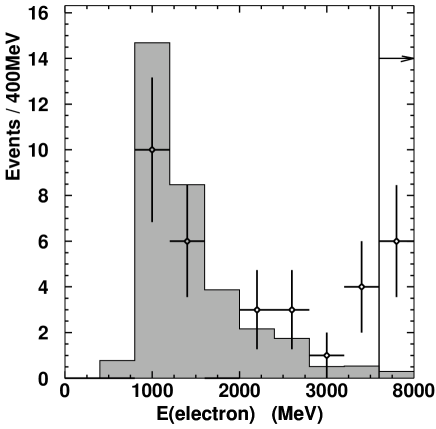
Figure 24: Electron energy spectrum for the candidates of $\nu_{e}$ interactions selected in SciBar. The MC spectrum (histogram) is normalized to the data separately for signal (30 events) and background (3 events). The contents of the highest energy bin is integrated between 3.6 and 8 GeV.

The consistency of the measurements in the LG and SciBar between themselves and with the MC predictions confirms the quality of the measurements and of the MC simulation. However, since the measurements are limited to a restricted energy region, for all the analyses described in the paper we use the $\nu_{e}$ component as given by the MC simulation.

VII Measurement of neutrino spectrum at the near detector

The neutrino energy spectrum before oscillation is measured with near detector 1KT, SciFi and SciBar CC event samples. The neutrino energy is reconstructed from the muon kinematics parameters $p_{\mu}$ and $\theta_{\mu}$ assuming a QE interaction as given in Eq. 2. The two-dimensional distributions of $p_{\mu}$ versus $\theta_{\mu}$ are used to measure the neutrino energy spectrum. The spectrum is fitted by using a $\chi^{2}$ method to compare observed ($p_{\mu}$, $\theta_{\mu}$) distributions to MC expectations.

VII.1 The fitting method

In order to obtain the neutrino energy spectrum, the ($p_{\mu}$, $\theta_{\mu}$) distribution is fit with the MC expectation as shown in Fig. 25. The neutrino energies are divided into eight bins as shown in Table 9. For the MC expectation, the $(p_{\mu},\theta_{\mu})$ distribution is prepared for each $E_{\nu}$ bin and separately for QE and nonQE interactions; $8\times 2$ distributions are prepared in total for each event sample.

The free parameters in the fit are the neutrino energy spectrum parameters for eight energy bins $(f^{\phi}_{1},...,f^{\phi}_{8})$ and a parameter, $R_{\mathrm{nQE}}$, which represents the relative weighting of CC-nonQE events to CC-QE events. The systematic uncertainties, such as nuclear effects, the energy scale, the track finding efficiency, and other detector related systematics, are also incorporated as the fitting parameters ($f$). The contents in $(m,n)$-th bin of the $(p_{\mu},\theta_{\mu})$ distribution, $N^{\mathrm{MC}}_{m,n}$, is expressed with the 16 templates and the fitting parameters as,

$$N^{\mathrm{MC}}_{m,n}\equiv P\cdot\sum_{i=1}^{8}f^{\phi}_{i}\cdot\left[N^{\mathrm{MC}(\mathrm{QE})}_{m,n,i}+R_{\mathrm{nQE}}\cdot N^{\mathrm{MC}(\mathrm{nQE})}_{m,n,i}\right],$$ (9)

where $P$, $N^{\mathrm{MC}(\mathrm{QE})}_{m,n,i}$ and $N^{\mathrm{MC}(\mathrm{nQE})}_{m,n,i}$ are a normalization parameter, the number of expected contents in the $(m,n)$-th bin for QE interaction and that for non-QE interaction for the $i$-th neutrino energy bin. We take the $\chi^{2}$ between the observed distributions, $N^{\mathrm{obs}}_{m,n}$, and $N^{\mathrm{MC}}_{m,n}$.

During the fit, the flux in each energy bin and $R_{\mathrm{nQE}}$ are re-weighted relative to the nominal values in the MC simulation. The flux for $E_{\nu}=1.0-1.5$ GeV bin is fixed to unity for the normalization, and another set of parameters is prepared for relative normalization of each detector.

The $\chi^{2}$ functions are separately defined for each detector and then summed to build a combined $\chi^{2}$ function as

$$\chi^{2}_{\mathrm{ND}}=\chi^{2}_{\mathrm{1KT}}+\chi^{2}_{\mathrm{SF}}+\chi^{2}_{\mathrm{SB}}$$ (10)

Finally, a set of the fitting parameters ($f^{\phi}_{i},R_{\mathrm{nQE}}:\mbox{\boldmath$f$}$) is found by minimizing the $\chi^{2}$ function. The best fit values, their error sizes and the correlations between them are used as inputs to the oscillation analysis, as described in Sec IX.1. The following subsections will describe the definition of $\chi^{2}$ for each subdetector and the results of fit.

Table 9: The $E_{\nu}$ interval of each bin.

	$f^{\phi}_{1}$	$f^{\phi}_{2}$	$f^{\phi}_{3}$	$f^{\phi}_{4}$	$f^{\phi}_{5}$	$f^{\phi}_{6}$	$f^{\phi}_{7}$	$f^{\phi}_{8}$
$E_{\nu}$ [GeV]	0.0$-$0.5	0.5$-$0.75	0.75$-$1.0	1.0$-$1.5	1.5$-$2.0	2.0$-$2.5	2.5$-$3.0	3.0$-$

VII.2 Definition of $\chi^{2}$ for 1KT

To measure the neutrino energy spectrum, we select a QE enriched data sample called the fully contained one-ring $\mu$-like (FC1R$\mu$) sample. In addition to the 1KT event rate selection (see Section VI.A), we require four additional conditions. These are that all visible particles are inside the 1KT detector (fully contained), one Cherenkov ring is found (one-ring), the particle identification is a muon ($\mu$-like), and the reconstructed muon momentum is greater than 200 MeV/$c$. This last condition is to ensure the quality of the event reconstruction. After these cuts, the fraction of CCQE events is about 60%. See Table 10 for the data summary and CCQE fraction. The requirement of full containment in the 1KT suppresses events at high momentum compared to the other detectors. Figs. 26, 27, and 28 show the ring number likelihood, particle identification likelihood, and the fully contained versus partially contained event (FC/PC) separation, respectively, used in the FC1R$\mu$ event selection. Any discrepancies between data and the MC simulation observed are used to estimate some of the systematic errors in the 1KT mentioned below.

Table 10: The summary table for the number of observed events in the FC1R$\mu$ sample, the efficiency and the purity of the CCQE events estimated with the MC simulation.

	# of events	CCQE efficiency (%)	CCQE purity (%)
FC1R$\mu$	52110	53.7	57.9

The selected data and the MC simulation are then binned into 2-dimensional distributions of muon momentum versus the scattering angle ($\theta_{\mu}$). The momentum is divided into 16 100 MeV/c bins from 0 - 1600 MeV/c. The scattering angle is divided into 10 bins where the first nine are in increments of 10 degrees from 0^∘-90^∘ and the final bin contains all events with the angle greater than 90^∘. The bins for which the expected number of events is greater than 10 are used for the analysis (80 bins in total).

The neutrino spectrum is derived by comparing the observed data and the weighted sum of Monte Carlo expectations using a $\chi^{2}$ test.

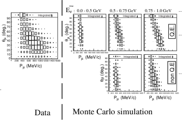
Figure 25: Schematic view of the binning of the data and Monte Carlo events for the spectrum fit. The left plot shows a correlation between $p_{\mu}$ and $\theta_{\mu}$ for FC1R$\mu$ events in the 1KT data used for the spectrum fit. The right plots show those for the MC sample separately prepared for each neutrino energy bin and for QE and non-QE interactions.

The $\chi^{2}$ is defined as:

$$\chi^{2}_{KT} = \sum_{m,n}\frac{\left(N^{\rm obs}_{m,n}-N^{\rm MC}_{m,n}\right)^{2}}{\sigma^{2}_{m,n}}+\frac{\left(1-\epsilon\right)^{2}}{\sigma^{2}_{energy}}$$ (11)

where $N^{\rm obs}_{m,n}$ is the number of observed events for data for $(m,n)$-th bin, $N^{\rm MC}_{m,n}$ is the number of MC events as given by equation 9, $\epsilon$ is the fitting parameter for energy scale ($\epsilon$ = 1 is a nominal value) which scales the muon momentum, $\sigma_{m,n}$ is the error including statistical and systematic errors, and $\sigma_{energy}$ is the estimated uncertainty of the energy scale, +3$/-$4%.

Figure 26: The distribution of ring counting likelihood for the 1KT. Those events that have a likelihood less than or equal to 0.0 are considered to have one ring; those above 0.0 are considered to be multi-ring. In this plot, data are the circles and the MC simulation is the histogram. The hatched histogram shows the CCQE component. Only statistical errors are shown for data.

Figure 27: The distribution of particle identification likelihood for the 1KT. The events with a likelihood greater than 0.0 are $\mu$-like while those less than or equal to 0.0 are e-like. Data are the circles and the MC simulation is the histogram with the CCQE component shown as the hatched area.

Figure 28: The largest charge in a PMT for a 1KT event. Events that have a charge less than 200 p.e. are considered FC events. The rest are PC events. Data are the circles and the MC simulation is the histogram, with the CCQE component shown as the hatched area.

The parameters $f^{\phi}_{i}$, $R_{\rm nQE}$, P, and $\epsilon$ are the fitting parameters as discussed above.

The systematic errors that are introduced in the fit come mainly from the event selection. Those errors are the ring counting likelihood, the particle identification likelihood, the FC/PC cut, the event vertex and direction reconstruction, and the energy scale. The other systematic errors are from the detector calibration and the axial vector mass ($M_{A}$), which is used for our neutrino interaction model.

VII.3 Definition of $\chi^{2}$ for SciFi

The SciFi tracking detector can observe charged particle tracks produced in neutrino-water interactions. Since SciFi uses the same target material (water) as 1KT and SK, systematic uncertainty due to different target nuclei is reduced. The data taken during K2K-Ib and K2K-IIa periods have been analyzed.

We choose charged current events in which a muon track starts from an interaction in the SciFi fiducial volume and stops in the MRD detector. The fiducial region is defined as a rectangle 1.1 $m$ to each side of the detector’s center in both $x$ and $y$, covering the first to 17^th water containers. The fiducial mass is 5.59 $\pm$ 0.07 metric tons. The primary (muon) track should match a hit in the downstream scintillator hodoscope, with no matching hit in the upstream one. It should also match a reconstructed track which has at least penetrated one piece of steel and produced hits in two layers in the MRD. The muon momentum threshold is 675 MeV/c for period-Ib and 550 MeV/c for period IIa.

For the K2K-Ib data, to enhance sensitivity to low energy neutrino interactions, we also include events in which the muon stops in the Lead Glass calorimeter (LG) and events which penetrate even single active layer in the MRD. Here, the response of the matched LG cluster should be greater than 100 MeV, which prevents proton tracks from being identified as muon tracks. By including these samples the $p_{\mu}$ threshold for period-Ib data is reduced to 400 MeV/c.

	Ib	IIa
Detector Configuration	SciFi+LG+MRD	SciFi+MRD
$\rm{POT_{SciFi}}$ ($\times$1018)	39.70	22.04
SciFi-MRD(track match)	6,935	5,188
SciFi-MRD(cell match only)	1,403	1,743∗
SciFi-LG	2,666	–

Table 11: Number of events in each event category observed in SciFi. ^∗The events are not used for the spectrum reconstruction.

The number of events for each event category, together with the total POT of the beam spills used for the analyses, are summarized in Table 11. In total 17,935 charged current candidate events have been collected for the data corresponding to $\rm{POT_{SciFi}}$=6.17$\times 10^{19}$ POT. After correcting for the changing detector configuration and efficiency, the event rate per POT was stable from month to month.

In the spectrum reconstruction, there must be one or two tracks in the event, including the muon; events with three or more tracks are discarded, which amounts to about 3% of the total. The two-track sample is further subdivided into a QE and a non quasi-elastic sample. For QE events, the muon momentum and muon angle are sufficient to predict the angle of the recoil proton because of the simple two-body kinematics. If the observed second track matches this prediction, within 25 degrees, then it is likely the event is QE. If the second track is more than 25 degrees from the predicted angle, then it is very likely not a QE event, as shown in Fig. 29.

Figure 29: Example of the distribution of $\Delta\theta_{P}$, the difference between the observed and predicted (assuming QE interaction) angle of the second track. This distribution is for SciFi 2-track events for the K2K-I period. The data (circles) and MC (histogram) are compared, and the shaded region shows the QE fraction in the MC.

Table 12: QE efficiency and QE purity of all events for K2K-I and K2K-IIa for each SciFi subsample, estimated from the MC before fitting.

	QE efficiency (%)		QE purity (%)
	K2K-I	K2K-IIa	K2K-I	K2K-IIa
1-track	39	36	50	57
QE	5	5	53	58
nonQE	2	2	11	12
total	46	42

The above data sample gives three subsamples each for K2K-I and K2K-IIa. Tab. 12 shows the QE efficiency (fraction of QE MC events ending up in each subsample) and QE purity (fraction of events in the subsample which are QE) for K2K-I and K2K-IIa. The LG stopping events are separated from the rest of the K2K-I data, giving another three subsamples – a total of nine. These samples are then divided into seven angle bins from 0 to 60 degrees, in 10 degree increments, and also into eight muon momentum bins, which have the same intervals as the neutrino energy bins in Tab. 9. The kinematics of these interactions are such that the bins at both high angle and high momentum contain neither data nor MC events and are not used in the analysis. The high muon thresholds also mean there are no data in the lowest energy region, and it is also not used in the fit.

In addition to the energy spectrum and R_nQE parameters, the fit includes several systematic parameters specific to the SciFi detector. Three refer to uncertainties in the reconstructed energy of each event. Since the muon momentum is reconstructed from the range of the muon, uncertainty in the material assay, and in the dE/dx used in the GEANT Monte Carlo simulation, as well as the uncertainty in the outgoing muon energy from a neutrino interaction, are important. A muon energy scale parameter $P^{\mathrm{SF}}_{\mathrm{Escale}}$ with an uncertainty of $\pm$2.7% is applied to the measured muon momenta. The second parameter $P^{\mathrm{SF}}_{\mathrm{LG-density}}$ accounts for an uncertainty of $\pm$ 5% in the muon energy loss specifically when it passes through the LG, and we consider this to be an uncertainty in the LG density. A final energy scale applies only to the energy reconstructed from the visible energy clusters in the LG for LG stopping events. This is expressed as the parameter $P^{\mathrm{SF}}_{\mathrm{LG-cluster}}$ and is given as an energy shift in GeV. The uncertainty used in the fit for the LG cluster energy calibration is $\pm$ 30 MeV. The muon momentum for LG stopping events is reconstructed only from the range in SciFi and the cluster energy observed in the LG.

There are two other systematic parameters: a migration between one-track and two-track events, $P^{\mathrm{SF}}_{\mathrm{2nd-track-eff}}$, which accounts for the tracking efficiency for short, second tracks; and a migration between the two-track QE and non-QE samples, $P^{\mathrm{SF}}_{\mathrm{rescattering}}$, to account for nuclear effects such as the uncertainty in the re-scattering of the proton as it leaves the nucleus from a QE interaction. Both parameters are simple linear migrations, and we take a 5% uncertainty in the former and a 2.5% uncertainty in the latter. They move a fraction of events from a particular $p_{\mu}$ and $\theta_{\mu}$ bin from one of the three subsamples to the same bin in another of the three subsamples.

There are 286 bins of SciFi data included in the fit, and six SciFi specific systematic parameters including normalization $P^{\mathrm{SF}}_{\mathrm{Norm}}$. Our $\chi^{2}$ is defined as the negative of the logarithm of the Poisson likelihood for the binned data, plus $\chi^{2}$ terms arising from the pull of five systematic errors (but not normalization):

$$\chi^{2} = -2\ln\lambda(\theta)$$ (12)

$$= 2\sum_{m,n}[N^{\mathrm{MC}}_{m,n}(\theta)-N^{\mathrm{obs}}_{m,n}+N^{\mathrm{obs}}_{m,n}\ln(N^{\mathrm{obs}}_{m,n}/N^{\mathrm{MC}}_{m,n}(\theta))]$$

$$+ \chi^{2}_{\mathrm{Escale}}+\chi^{2}_{\mathrm{LG\ density}}+\chi^{2}_{\mathrm{LG\ cluster\ energy}}$$

$$+ \chi^{2}_{\mathrm{2nd\ track\ eff}}+\chi^{2}_{\mathrm{Rescattering}}.$$

in which $N^{\mathrm{MC}}_{m,n}(\theta)$ and $N^{\mathrm{obs}}_{m,n}$ are the predicted and observed values in the (m,n)-th bin for some values of the parameters $\theta$. This is the simplified version given in Ref. Eidelman et al. (2004) and its minimum follows a $\chi^{2}$ distribution. To this, we add $\chi^{2}$ terms arising from the systematic errors.

VII.4 Definition of $\chi^{2}$ for SciBar

The CC event selection in the SciBar detector is similar to that of the SciFi detector. The fiducial volume of SciBar is defined as a rectangle that extends $2.6\times 2.6$ m² around the beam axis, from the second to 53^rd layer of scintillator. The fiducial mass is 9.38 tons. Events with any track starting in the SciBar fiducial volume and matched with a track or hits in the MRD are selected as CC candidates (SciBar-MRD sample). This requirement imposes a threshold of 450 MeV/c on $p_{\mu}$, reconstructed from its range through SciBar and MRD. According to the MC simulation, 98% of the events selected by this requirement are CC induced events, and the rest are neutral current (NC) interactions accompanied by a charged pion or proton which penetrates into the MRD. The $p_{\mu}$ resolution, $p_{\mu}$ scale uncertainty and $\theta_{\mu}$ resolution are 80 MeV/c, 2.7% and 1.6 degrees, respectively.

Events with one or two reconstructed tracks are selected from the SciBar-MRD sample. The two-track events are subdivided into two categories — QE samples and nonQE samples — by using kinematic information, $\Delta\theta_{p}$, like SciFi. The number of observed events and the fraction and efficiency of QE interactions estimated with the MC simulation for each event category are summarized in Table 13.

Table 13: Number of observed events in each event category and the efficiency and purity of the QE events estimated with the MC simulation for the SciBar detector.

	# events	QE efficiency (%)	QE purity (%)
1-track	7256	50.0	57.8
QE	1760	15.4	71.3
nQE	2014	3.7	15.9
Total	11030	69.1	—

The SciBar term of the $\chi^{2}$ consists of two components,

$$\chi^{2}_{\mathrm{SB}}=\chi^{2}_{\mathrm{dist}}+\chi^{2}_{\mathrm{syst}}.$$ (13)

The $\chi^{2}_{\mathrm{dist}}$ is calculated by the binned likelihood method using the $(p_{\mu},\theta_{\nu})$ distribution. The bin widths are 0.1 GeV/c for $p_{\mu}$ and 10 degrees for $\theta_{\mu}$. Bins with the expected number of events greater than five are used for the fit. In total, 239 bins are used for the analysis. The number of observed events in each bin, $N^{\mathrm{obs}}_{m,n}$, is assumed to follow a Poisson distribution with the mean $N^{\mathrm{MC}}_{m,n}$. A bin-by-bin systematic uncertainty on hadron contamination is implemented by the convolution of a Poisson with a Gaussian distribution. The $\chi^{2}_{\mathrm{dist}}$ is thus defined as:

$$\chi^{2}_{\mathrm{dist}}=-2\sum_{m,n}\ln\frac{\mathcal{L}\left(N^{\mathrm{obs}}_{m,n};N^{\mathrm{MC}}_{m,n};\mathbf{\sigma}\right)}{\mathcal{L}\left(N^{\mathrm{obs}}_{m,n};N^{\mathrm{obs}}_{m,n};\mathbf{\sigma}\right)},$$ (14)

$$\mathcal{L}\left(N^{\mathrm{obs}}_{m,n};N^{\mathrm{MC}}_{m,n};\mathbf{\sigma}\right)\equiv$$

$$~{}~{}~{}\prod_{m,n}\int^{\infty}_{0}\frac{1}{\sqrt{2\pi}\sigma_{m,n}}\exp\left[-\frac{\left(x-N^{\mathrm{MC}}_{m,n}\right)^{2}}{2\sigma^{2}_{m,n}}\right]\cdot\frac{x^{N^{\mathrm{obs}}_{m,n}}e^{-x}}{N^{\mathrm{obs}}_{m,n}!}dx.$$

The normalization parameter of each sample is given by

$$P^{\mathrm{Norm}}_{\mathrm{1track}} = P^{\mathrm{SB}}_{\mathrm{Norm}}$$ (16)

$$P^{\mathrm{Norm}}_{\mathrm{QE}} = P^{\mathrm{SB}}_{\mathrm{Norm}}\cdot P^{\mathrm{SB}}_{\mathrm{2trk/1trk}}$$ (17)

$$P^{\mathrm{Norm}}_{\mathrm{nonQE}} = P^{\mathrm{SB}}_{\mathrm{Norm}}\cdot P^{\mathrm{SB}}_{\mathrm{2trk/1trk}}\cdot P^{\mathrm{SB}}_{\mathrm{nonQE/QE}}$$ (18)

where $P^{\mathrm{SB}}_{\mathrm{Norm}}$ is the overall normalization factor, and $P^{\mathrm{SB}}_{\mathrm{2trk/1trk}}$ and $P^{\mathrm{SB}}_{\mathrm{nonQE/QE}}$ are the parameters to vary the ratio of the number of 2-track events to that of 1-track events and the ratio of the number of CC-nonQE events to that of CC-QE events, respectively, within their systematic uncertainties. We consider the uncertainties from nuclear effects and detector systematics. The possible difference between carbon and oxygen is included in the nuclear effect uncertainty. Because the nuclear effects are common source of the uncertainties for $P^{\mathrm{SB}}_{\mathrm{2trk/1trk}}$ and $P^{\mathrm{SB}}_{\mathrm{nonQE/QE}}$, their correlation is also estimated. In addition, $P^{\mathrm{SB}}_{\mathrm{p-scale}}$ is introduced to account for the uncertainty of the energy scale of the muon reconstruction. The momentum scale uncertainty is 2.7% as described above.

The $\chi^{2}_{\mathrm{syst}}$ is calculated with constraint parameters, including their correlation:

$$\chi^{2}_{\mathrm{syst}} = (\mbox{\boldmath$P_{syst}$}-\mbox{\boldmath$P_{0}$})^{t}\mbox{\boldmath$V^{-1}$}(\mbox{\boldmath$P_{syst}$}-\mbox{\boldmath$P_{0}$})$$ (19)

where $P_{\mathrm{syst}}$ represents a set of systematic parameters, $P_{0}$ are their nominal values, and $V$ is a covariance matrix. Three systematic parameters , $P^{\mathrm{SB}}_{\mathrm{p-scale}}$, $P^{\mathrm{SB}}_{\mathrm{2trk/1trk}}$, and $P^{\mathrm{SB}}_{\mathrm{nonQE/QE}}$ are included in $P_{\mathrm{syst}}$; they are defined as relative weighting factors to the nominal MC expectation and all components of $P_{0}$ are set to unity. The uncertainties and correlation among the parameters are evaluated to be

$$\mathbf{V}\equiv\bordermatrix{&P^{\mathrm{SB}}_{\mathrm{p-scale}}&P^{\mathrm{SB}}_{\mathrm{2trk/1trk}}&P^{\mathrm{SB}}_{\mathrm{nonQE/QE}}\cr P^{\mathrm{SB}}_{\mathrm{p-scale}}&+(0.027)^{2}&0&0\cr P^{\mathrm{SB}}_{\mathrm{2trk/1trk}}&0&+(0.059)^{2}&+(0.017)^{2}\cr P^{\mathrm{SB}}_{\mathrm{nonQE/QE}}&0&+(0.017)^{2}&+(0.058)^{2}}.$$ (20)

The dominant error sources are track finding efficiency for $P^{\mathrm{SB}}_{\mathrm{2trk/1trk}}$ and the nuclear effects uncertainty for $P^{\mathrm{SB}}_{\mathrm{nonQE/QE}}$.

VII.5 Fit results

The minimum $\chi^{2}$ point in the multi-parameter space is found by changing the spectrum shape, $R_{\mathrm{nQE}}$ and the systematic parameters, where the MINUIT program library James and Roos (1975) is employed. The central values and the errors of the fitting parameters are summarized in Table 14. All the systematic parameters stay within their estimated errors. The result of the spectrum measurement is shown in Fig. 30 with the prediction of the beam MC simulation.

The results of the measurements with individual detector data are also shown in Table 14. In the fit with only 1KT data, the energy spectrum parameters are fixed to their default values for the high energy region where there is little or no acceptance. For the same reason, the low energy region is fixed for SciFi and SciBar. All the fitting parameters are in good agreement within their errors each other except for $R_{\mathrm{nQE}}$.

The $p_{\mu}$, $\theta_{\mu}$ and $q^{2}_{\mathrm{rec}}$ distributions for the 1KT, SciFi and SciBar samples are shown in Fig. 33–33. In these figures, the reconstructed $Q^{2}$ distributions($q^{2}_{\mathrm{rec}}$) are constructed by assuming that the interaction was CC-QE and using the reconstructed energy under this assumption. The expected distributions of the MC simulation with the best-fit parameters are also shown. The MC simulation reproduces all the distributions well.

The discrepancy in $R_{\mathrm{nQE}}$ is treated as a systematic error. However, the value of $R_{\mathrm{nQE}}$ is strongly correlated with the $E_{\nu}$ spectrum as well as the other systematic parameters such as $P^{\mathrm{SB}}_{\mathrm{nonQE/QE}}$. In order to evaluate $R_{\mathrm{nQE}}$ with each detector data set under identical fitting condition, a second fit is performed. In the second fit, the $E_{\nu}$ spectrum and the systematic parameters, except for the overall normalization, are fixed at the best fit values obtained with all the three detectors. The best fit value of $R_{\mathrm{nQE}}$ for each detector in the second fit is (1KT, SciFi, SciBar) = (0.76, 0.99, 1.06), respectively, while the fit result with three detectors is 0.96. Therefore, an additional error of 0.20 is assigned to $R_{\mathrm{nQE}}$ in order to account for the discrepancy.

The errors of the measurement are provided in the form of an error matrix. Correlations between the parameters are taken into account in the oscillation analysis with this matrix. The full elements in the error matrix are shown in Table 15.

Table 14: Results of the spectrum measurement. The best fit value of each parameter is listed for the fits with all the detectors’ data, with the 1KT data, with the SciFi data and with the SciBar data, respectively. The reduced $\chi^{2}$ ($\chi^{2}_{\mathrm{total}}$/DOF) and the averaged $\chi^{2}$ of each detector ($\chi^{2}$/N_bin) are also shown.

parameter	Combined	1KT only	SciFi only	SciBar only
$f_{1}$ (0.00-0.50 GeV)	$\mathbf{1.657\pm 0.437}$	$2.372\pm 0.383$	$\equiv 1$	$\equiv 1$
$f_{2}$ (0.50-0.75 GeV)	$\mathbf{1.107\pm 0.075}$	$1.169\pm 0.072$	$0.882\pm 0.317$	$1.166\pm 0.251$
$f_{3}$ (0.75-1.00 GeV)	$\mathbf{1.154\pm 0.061}$	$1.061\pm 0.065$	$1.157\pm 0.201$	$1.145\pm 0.134$
$f_{4}$ (1.00-1.50 GeV)	$\mathbf{\equiv 1}$	$\equiv 1$	$\equiv 1$	$\equiv 1$
$f_{5}$ (1.50-2.00 GeV)	$\mathbf{0.911\pm 0.044}$	$0.709\pm 0.151$	$0.980\pm 0.107$	$0.963\pm 0.070$
$f_{6}$ (2.00-2.50 GeV)	$\mathbf{1.069\pm 0.059}$	$\mathbf{\equiv 1}$	$1.188\pm 0.096$	$0.985\pm 0.086$
$f_{7}$ (2.50-3.00 GeV)	$\mathbf{1.152\pm 0.142}$	$\mathbf{\equiv 1}$	$1.062\pm 0.230$	$1.291\pm 0.283$
$f_{8}$ (3.00- GeV)	$\mathbf{1.260\pm 0.184}$	$\equiv 1$	$1.323\pm 0.203$	$1.606\pm 0.749$
$R_{\mathrm{nQE}}$	$\mathbf{0.964\pm 0.035}$	$0.589\pm 0.071$	$1.069\pm 0.060$	$1.194\pm 0.092$
$\mathrm{P}^{\mathrm{1kt}}_{\mathrm{Norm}}$	$\mathbf{0.948\pm 0.024}$	$1.172\pm 0.046$	—	—
$\mathrm{P}^{\mathrm{1kt}}_{\mathrm{energy}}$	$\mathbf{0.984\pm 0.004}$	$0.993\pm 0.007$	—	—
$\mathrm{P}^{\mathrm{SF}}_{\mathrm{Norm}}$	$\mathbf{1.009\pm 0.029}$	—	$0.925\pm 0.058$	—
$\mathrm{P}^{\mathrm{SF}}_{\mathrm{Escale}}$	$\mathbf{0.980\pm 0.006}$	—	$0.980\pm 0.007$	—
$\mathrm{P}^{\mathrm{SF}}_{\mathrm{LG-density}}$	$\mathbf{0.929\pm 0.012}$	—	$0.928\pm 0.012$	—
$\mathrm{P}^{\mathrm{SF}}_{\mathrm{LG-cluster}}~{}[\mathrm{GeV}]$	$\mathbf{-0.001\pm 0.002}$	—	$-0.002\pm 0.003$	—
$\mathrm{P}^{\mathrm{SF}}_{\mathrm{2nd-track-eff}}$	$\mathbf{0.959\pm 0.014}$	—	$0.932\pm 0.017$	—
$\mathrm{P}^{\mathrm{SF}}_{\mathrm{rescattering}}$	$\mathbf{1.048\pm 0.055}$	—	$0.993\pm 0.062$	—
$\mathrm{P}^{\mathrm{SB}}_{\mathrm{Norm}}$	$\mathbf{0.998\pm 0.010}$	—	—	$1.003\pm 0.011$
$\mathrm{P}^{\mathrm{SB}}_{\mathrm{p-scale}}$	$\mathbf{0.976\pm 0.004}$	—	—	$0.972\pm 0.004$
$\mathrm{P}^{\mathrm{SB}}_{\mathrm{2trk/1trk}}$	$\mathbf{0.953\pm 0.021}$	—	—	$0.961\pm 0.023$
$\mathrm{P}^{\mathrm{SB}}_{\mathrm{nonQE/QE}}$	$\mathbf{1.066\pm 0.032}$	—	—	$0.978\pm 0.040$
$\chi^{2}_{\mathrm{total}}$/DOF	687.2 / 585	46.8 / 73	328.7 / 273	253.3 / 228
$\chi^{2}_{\mathrm{1kt}}$/Nbin	85.4 / 80	47.7 / 80	—	—
$\chi^{2}_{\mathrm{SciFi}}$/Nbin	335.6 / 286	—	328.7 / 286	—
$\chi^{2}_{\mathrm{SciBar}}$/Nbin	266.1 / 239	—	—	253.3 / 239

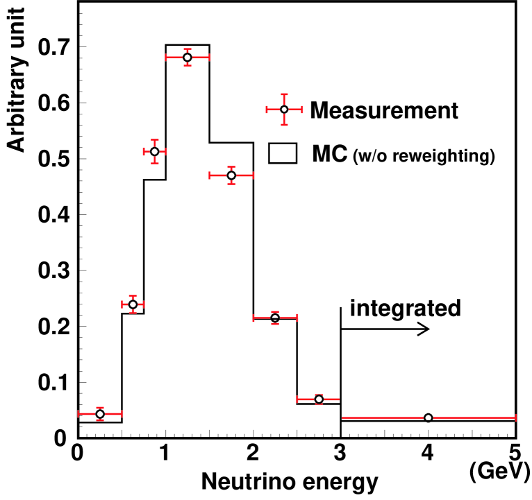
Figure 30: The neutrino energy spectrum measured at the near site, assuming CC-QE. The expectation with the MC simulation without reweighting is also shown.

Table 15: The error matrix for $f_{\mathrm{i}}$ and $R_{\mathrm{nQE}}$. The square root of error matrix (sign $\left[{M_{ij}}\right]\cdot\sqrt{|M_{ij}|}$) is shown here in the unit of %.

	$f_{1}$	$f_{2}$	$f_{3}$	$f_{5}$	$f_{6}$	$f_{7}$	$f_{8}$	$R_{\mathrm{nQE}}$
$f_{1}$	43.86	-3.16	7.28	-2.21	-0.76	-3.48	0.81	-8.62
$f_{2}$	-3.16	7.51	1.97	1.90	0.62	1.29	2.43	-5.68
$f_{3}$	7.28	1.97	6.00	3.38	1.63	3.44	1.71	-2.99
$f_{5}$	-2.21	1.90	3.38	4.04	-1.86	4.53	2.20	1.65
$f_{6}$	-0.76	0.62	1.63	-1.86	5.28	-5.85	5.11	0.94
$f_{7}$	-3.48	1.29	3.44	4.53	-5.85	13.67	-10.14	4.09
$f_{8}$	0.81	2.43	1.71	2.20	5.11	-10.14	18.35	-11.77
$R_{\mathrm{nQE}}$	-8.62	-5.68	-2.99	1.65	0.94	4.09	-11.77	20.30

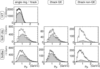
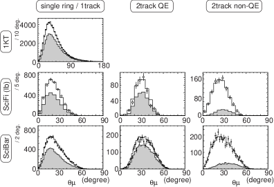
Figure 31: The $p_{\mu}$ distributions for each event sample of all near detectors with the MC simulation after fitting, given by open histograms. The hatched areas are the CCQE components in the MC distributions.

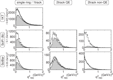
Figure 32: The $\theta_{\mu}$ distributions for each event sample of all near detectors with the MC simulation after fitting, given by open histograms. The hatched areas are the CCQE components in the MC distributions.

Figure 33: The $q^{2}_{\mathrm{rec}}$ distributions for each event sample of all near detectors with the MC simulation after fitting, given by open histograms. The hatched areas are the CCQE components in the MC distributions.

VIII SK data

VIII.1 SK data reduction

Beam-induced neutrino events in SK are selected according to criteria described in this section. Following selection, events which are fully contained in the SK fiducial volume are reconstructed using similar methods to the SK atmospheric neutrino analysis and then used in the K2K oscillation analysis.

In order to select those neutrino interactions which come from the accelerator at KEK, two Universal Time Coordinated time stamps from the worldwide GPS system are compared. Both $T_{KEK}$ for the KEK-PS beam spill start time, and $T_{SK}$ for the SK trigger time are recorded. The time difference $\Delta T=T_{SK}-T_{KEK}-TOF$, where $TOF$ is a time of flight, is distributed from 0 and 1.1 $\mu sec$ matching the timing width of the beam spill of the KEK-PS. The maximum difference of the synchronization between two sites is measured to be less than 200 ns by using an external atomic clock. For this reason we require the $\Delta T$ for selected events to be between -0.2 to 1.3 $\mu$ sec.

Table 16: SK event reduction summary.

Reduction step	K2K-I	K2K-II
${\rm|\Delta T|<500\mu sec}$,	107892	470469
no pre-activity
total number of p.e. within	36560	16623
300 n sec timing window
$>$200(K2K-I),94(K2K-II)
Fully contained event	153	99
flasher cuts	97	88
visible Energy $>$30MeV	95	85
fiducial volume cut	56	59
${\rm|\Delta T|=-0.2-1.3\mu sec}$	55	57

Table 17: SK event summary. For oscillated expectations, ${\rm sin^{2}2\theta=1}$ and ${\rm\Delta m^{2}=2.8\times 10^{-3}eV^{2}}$ are assumed.

	K2K-I			K2K-II
	data	expected		data	expected
		w/o osc.	w/ osc.		w/o osc.	w/ osc.
Fully contained	55	80.8	54.8	57	77.3	52.4
1-ring	33	51.0	31.1	34	49.7	30.5
$\mu$-like	30	47.1	27.7	28	45.2	26.7
e-like	3	3.9	3.4	6	4.5	3.8
multi-ring	22	29.8	23.7	23	27.6	21.9

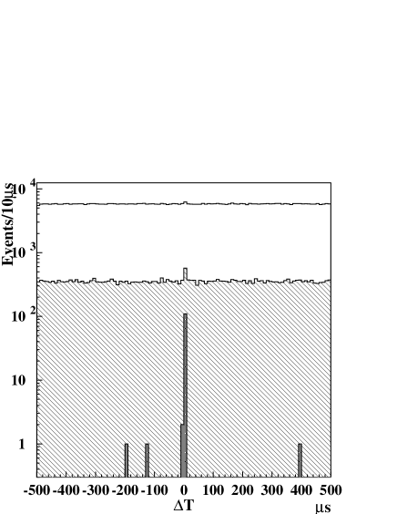
Figure 34: The $\Delta T$ distribution at each reduction step. Clear, hatched and shaded histograms are after pre-activity cut, total p.e. cut, and fiducial volume cut, respectively.

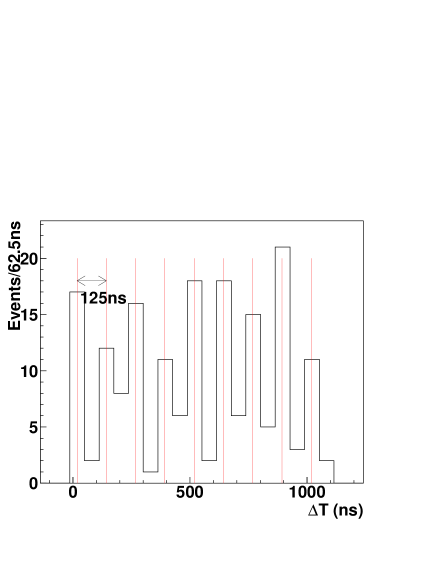
Figure 35: The $\Delta T$ distribution for fully contained events. The nine micro-bunch structure present in the beam is clearly seen.

In addition to the timing criteria, the following cuts are required:

1. In order to remove decay-electrons from the sample, events must have no activity in the 30 $\mu$s before the event.

2. There must be a minimum number of photo-electrons seen within a 300 ns timing window. The required number of photo-electrons are 200 for K2K-I and 94 for K2K-II.

3. Fully contained events are selected by requiring no activity in the outer detector.

4. A selection is made to remove events with PMTs which sometimes begin to produce light because of a discharge around the dynode. These events have easily identified characteristics such as a timing distribution which is much broader than neutrino events, and a repeating pattern of light in the detector.

5. At least 30 MeV energy must be deposited in the inner detector.

6. The events are selected to come from the 22.5 kiloton fiducial volume by requiring the reconstructed vertex position be at least 2m away from the inner detector wall.

Tab. 16 shows the reduction summary for K2K-I and K2K-II. The efficiency for these cuts are 77.2% for K2K-I and 77.9% for K2K-II. The majority of the inefficiency is due to NC interactions which are not selected by these criteria. In total, 112 accelerator produced, fully contained events, are observed in the SK fiducial volume, with 58 events reconstructed as 1-ring $\mu$-like. Tab. 17 summarizes the characterization of these events and the MC expectations with and without neutrino oscillation.

Figure 34 shows the $\Delta T$ distribution at each reduction step. A clear peak at $\Delta T=0$ is seen after the fiducial volume cut. Three off-timing fully contained events are observed within ${\rm\pm 500\mu sec}$ timing window which is consistent with the 2 expected background events from atmospheric neutrinos. In addition, the nine-bunch timing structure of the beam can be clearly seen in the $\Delta T$ distribution if finer bins are used as in Fig. 35. Fig. 36 shows the event rate as a function of POT. A KS-test performed against the assumption that the rate is proportional to POT gives a probability of 79%.

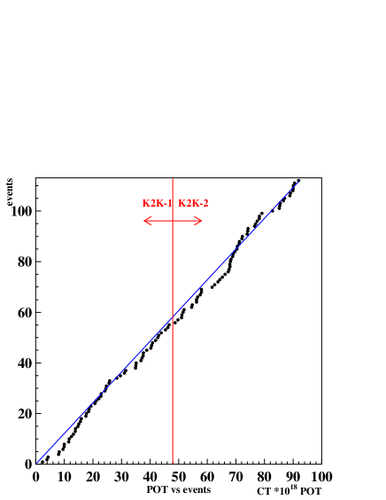
Figure 36: Event rate as a function of POT. The KS-test probability to observe our event rate under the assumption that the event rate is proportional to POT is 79%.

The energy distribution of the events is compared against expectation in several ways. Fig. 37 shows the visible energy distribution, which is estimated from the energy deposit in the inner detector for all of the fully contained fiducial volume events. In this figure, the observed data is compared with the MC expectation based on the ND measurement without neutrino oscillation.

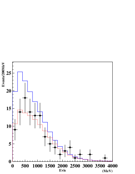
Figure 37: The visible energy distribution for fully contained fiducial-volume events in SK. The closed circles are the observed data. The solid histogram is the MC expectation based on the ND measurement without neutrino oscillation, and the dashed one is the MC expectation with neutrino oscillation of ${\rm sin^{2}2\theta=1}$ and ${\rm\Delta m^{2}=2.8\times 10^{-3}eV^{2}}$.

Figure 38 shows the expected energy spectrum together with the observation for the one-ring $\mu$-like events. The expectation is normalized by the number of observed events (58). The neutrino energy is reconstructed using the reconstructed muon momentum and the known beam-direction while assuming there was a QE interaction and ignoring the Fermi momentum. As can be seen, compared to the MC expectation there is a deficit of 1R$\mu$ events in the low energy region, as is expected from the oscillation hypothesis.

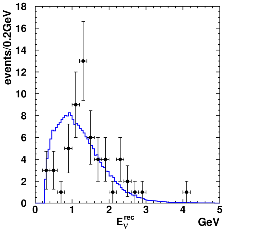
Figure 38: The reconstructed $E_{\nu}$ distribution for the SK 1-ring $\mu$-like sample. Points with error bars are data. The solid line is the expectation without oscillation. The histogram is normalized by the number of events observed (58).

VIII.2 Systematic error from reconstruction at SK

The systematic uncertainties for estimating ${\rm N_{SK}}$ and the reconstructed neutrino energy in SK are evaluated using atmospheric neutrinos as a control sample. Tab. 18 shows the systematic errors for ${\rm N_{SK}}$. The dominant uncertainty for estimating ${\rm N_{SK}}$ comes from the vertex reconstruction. Since a cut is made on fiducial volume a systematic shift in or out of this volume will either over or underestimate the number of events expected. It is evaluated comparing the number of events for atmospheric neutrino data with the MC expectation in the fiducial volume using two different vertex reconstruction programs.

Systematic errors due to the reconstruction algorithms themselves are also taken into account in the oscillation analysis. Systematic errors due to reconstruction are shown in table 19. Uncertainties coming from the ring counting and particle identification are evaluated by comparing the likelihood distributions for data and MC, and varying the selection criteria. Figure 39 and 40 show the ring counting and particle identification likelihood distributions of atmospheric neutrino data compared with the MC expectations in SK-II. The MC expectations reproduce the data well. The uncertainty for the energy scale are also estimated by using cosmic ray muons, the $\pi^{0}$ invariant mass and decay electrons. The energy scale uncertainty at SK is estimated to be 2.0% for K2K-I and 2.1% for K2K-II.

Table 18: Systematic errors for ${\rm N_{SK}}$.

	K2K-I	K2K-II
reduction	$<$1%	$<$1%
fiducial volume cut	2%	2%
decay electron background	0.1%	0.1%
MC statistics	0.6%	0.6%
Total	3%	3%

Table 19: Systematic errors for reconstructed neutrino energy spectrum. The errors are shown in %, and the five columns refer to different bins of neutrino energy, as shown in the table in units of GeV.

K2K-I (GeV)	0-0.5	0.5-1.0	1.0-1.5	1.5-2.0	2.0-
ring counting	3.4%	2.7%	3.0%	4.5%	4.5%
particle ID	0.9%	0.3%	0.5%	0.4%	0.4%
vertex	2.0%	2.0%	2.0%	2.0%	2.0%
total	4.1%	3.4%	3.6%	4.9%	4.9%
K2K-II (GeV)	0-0.5	0.5-1.0	1.0-1.5	1.5-2.0	2.0-
ring counting	5.3%	4.1%	3.7%	3.8%	3.8%
particle ID	2.6%	0.4%	0.3%	0.6%	0.6%
vertex	2.0%	2.0%	2.0%	2.0%	2.0%
total	6.2%	4.6%	4.2%	4.3%	4.3%

Figure 39: Ring counting likelihood distribution for SK-II atmospheric fully contained neutrino events. Closed circles are data and the histogram is MC expectation normalized by live time assuming neutrino oscillation at atmospheric best-fit parameters. Events with Likelihood $<$ 0 are assigned to be one-ring.

Figure 40: Particle identification likelihood distribution for SK-II atmospheric fully contained one-ring events. Closed circles are data and the histogram is MC expectation normalized by live time assuming neutrino oscillation at atmospheric best-fit parameters. Events with Likelihood $<$ 0 are assigned to be e-like.

IX Neutrino Oscillation Analysis

IX.1 Oscillation analysis method

A two-flavor neutrino oscillation analysis is performed based on a comparison between the observation and the expectation by use of a maximum-likelihood method. The signatures of neutrinos oscillating from $\nu_{\mu}$ to $\nu_{\tau}$ are both a reduction in the total number of observed neutrino events and a distortion in the neutrino energy spectrum. Thus, the likelihood function is defined as the product of the likelihoods for the observed number of events in the SK fiducial volume ($\mathcal{L}_{\mathrm{norm}}$) and the shape of the $E_{\nu}^{\mathrm{rec}}$ spectrum ($\mathcal{L}_{\mathrm{shape}}$). In addition, the systematic uncertainties are also treated as fitting parameters in the likelihood. They are included in a constraint likelihood term ($\mathcal{L}_{\mathrm{syst}}$) where they are varied within their uncertainties, thus modifying the expectation. The total likelihood function is then defined as:

$$\mathcal{L} = \mathcal{L}_{\mathrm{norm}}\times\mathcal{L}_{\mathrm{shape}}\times\mathcal{L}_{\mathrm{syst}}.$$ (21)

The oscillation parameters, $\Delta m^{2}$ and $\sin^{2}2\theta$, are obtained by maximizing the likelihood function. One-hundred twelve FC events are used in $\mathcal{L}_{\mathrm{norm}}$ and fifty eight FC 1R$\mu$ events are used for $\mathcal{L}_{\mathrm{shape}}$, respectively. The systematic parameters in the likelihood consist of the neutrino energy spectrum at the near detector site, the $F/N$ flux ratio, the neutrino-nucleus cross-section, the efficiency and the energy scale of SK, and the overall normalization.

IX.2 Prediction of the number of events and the energy spectrum at Super-Kamiokande

IX.2.1 Number of neutrino events

The expected number of neutrino events in SK ($N^{\mathrm{SK}}_{\mathrm{exp}}$) is derived by extrapolating the measured number of interactions in the 1KT ($N^{\mathrm{1KT}}_{\mathrm{int}}$, calculated in Eq. 8) with the ratio of the expected neutrino event rate per unit mass, $\rho^{\mathrm{SK}}/\rho^{\mathrm{1KT}}$. Taking into account the difference of fiducial mass ($M$) and the number of protons on target (POT) used in the analysis for 1KT and SK, $N^{\mathrm{SK}}_{\mathrm{exp}}$ is written as:

$$N^{\mathrm{SK}}_{\mathrm{exp}}(\Delta m^{2},\sin^{2}2\theta)\\ \equiv N^{\mathrm{1KT}}_{\mathrm{int}}\cdot\frac{\rho^{\mathrm{SK}}}{\rho^{\mathrm{1KT}}}\cdot\frac{\mathrm{M}^{\mathrm{SK}}}{\mathrm{M}^{\mathrm{1KT}}}\cdot\frac{\mathrm{POT}^{\mathrm{SK}}}{\mathrm{POT}^{\mathrm{1KT}}}\cdot C_{\nu_{e}},$$ (22)

where superscripts “1KT” and “SK” denote the variable for SK and 1KT, respectively, and $C_{\nu_{e}}$ is the correction factor for the difference of the electron neutrino contamination in the neutrino beam at 1KT and SK. The value of $C_{\nu_{e}}$ is estimated to be 0.996 with the MC simulation.

The expected event rate at each detector, $\rho$, is calculated from the neutrino flux $\Phi$, the neutrino-water interaction cross-section $\sigma$, and the detector efficiency $\epsilon$ estimated with the MC simulation:

$$\rho=\int dE_{\nu}\Phi(E_{\nu})\cdot\sigma(E_{\nu})\cdot\epsilon(E_{\nu}).$$

In order to account for the systematic uncertainty, we classify the neutrino interaction into three categories: CC-QE, CC-nonQE and NC. The event rate is calculated separately for each of the three interaction types and then summed. The neutrino flux at SK, $\Phi^{\mathrm{SK}}$, is estimated from the F/N flux ratio $R^{\mathrm{F/N}}$and the measured ND spectrum $\Phi^{\mathrm{ND}}$:

$$\Phi^{\mathrm{SK}}=R^{\mathrm{F/N}}(E_{\nu})\cdot\Phi^{\mathrm{ND}}(E_{\nu})\cdot(1-P(E_{\nu};\Delta m^{2},\sin^{2}2\theta)),$$

where $P(E_{\nu};\Delta m^{2},\sin^{2}2\theta)$ is the neutrino oscillation probability given by Eq. (1).

The uncertainties of $\Phi^{\mathrm{ND}}$ and their correlation are obtained from the ND analysis as shown in Tab. 15. Those for $R^{\mathrm{F/N}}$ are derived from the HARP $\pi^{+}$ measurement and the beam MC simulation, and are summarized in Tab. 5. In order to be insensitive to the absolute cross-section uncertainty, we incorporate the uncertainties in neutrino-nucleus cross-section as the cross-section ratio relative to CC-QE interactions. The uncertainty of the CC-nonQE/CC-QE cross-section ratio is taken from the ND measurements. For the NC/CC-QE cross-section ratio, we assign 11% uncertainty to NC single $\pi^{0}$ production based on the measurement with the 1KT Nakayama et al. (2005). The other NC interaction modes are assigned 30% uncertainty based on past experiments Monsay (1978). Taking into account the detection efficiency in SK, 15% is assigned as the net uncertainty on NC/CC-QE ratio. The uncertainties from event reconstruction at SK are summarized in Tab. 18. The uncertainty of the overall normalization of the number of events in each period is estimated from the fiducial mass error of 1KT and SK and the uncertainty in the difference of the number of protons on target used for the analysis. In total, the normalization error is estimated to be $\pm 5.1$% for both Ib and II periods.

For the period Ia, the beam configuration is different from other periods and we do not have a ND measurement of the energy spectrum. We employ different treatment of the systematic errors for this period. All the uncertainties, including those from the $F/N$ flux ratio, energy spectrum and cross-section, are incorporated into the error of the single normalization parameter. The total normalization uncertainty for the Ia period is estimated to be +9.0/-9.8%. The largest contribution to this uncertainty is from the energy spectrum, which is estimated with the HARP $\pi^{+}$ measurement and the beam MC simulation and gives $+5.8$%/$-7.0$%. Other contributions come from the $F/N$ flux ratio ($\pm 4.3$%) and the fiducial volume uncertainties of 1KT ($\pm 4.3$%) and SK ($\pm 3.0$%).

We estimate the expected number of events without neutrino oscillation while incorporating all of the known systematic uncertainties by use of a MC technique. Many sets of the systematic parameters are randomly generated with proper consideration of their correlation. For each systematic parameter set, $N^{\mathrm{SK}}_{\mathrm{exp}}$ is calculated using Equation (22), setting oscillation parameters to zero. The number of FC events without neutrino oscillation is estimated to be $158.1^{+9.2}_{-8.6}$. This technique allows us to determine the contributions from the individual systematics to the the total error by selectively including only some errors during the generation. We find that the dominant error sources are the fiducial volume uncertainties in 1KT and SK $\left({}^{+4.9\%}_{-4.8\%}\right)$ and the $F/N$ ratio $\left({}^{+2.9\%}_{-2.9\%}\right)$.

IX.2.2 Reconstructed neutrino energy spectrum

The expected spectrum shape of the reconstructed neutrino energy at SK, $\phi_{\mathrm{exp}}^{\mathrm{SK}}(E_{\nu}^{\mathrm{rec}})$, is calculated as:

$$\phi_{\mathrm{exp}}^{\mathrm{SK}}=\int dE_{\nu}\cdot\Phi^{\mathrm{SK}}(E_{\nu})\cdot\sigma(E_{\nu})\cdot\epsilon_{1\mathrm{R}\mu}^{\mathrm{SK}}(E_{\nu})\cdot r(E_{\nu};E_{\nu}^{\mathrm{rec}}),$$ (23)

where $\epsilon_{1\mathrm{R}\mu}^{\mathrm{SK}}$ is the detection efficiency for 1R$\mu$ events in SK and $r(E_{\nu};E_{\nu}^{\mathrm{rec}})$ is the probability of reconstructing an event with true energy $E_{\nu}$ as $E_{\nu}^{\mathrm{rec}}$. Both of them are estimated with the MC simulation. In the actual procedure, the $E_{\nu}$ and $E_{\nu}^{\mathrm{rec}}$ are binned with an interval of 50 MeV, and hence the integral over the true neutrino energy is replaced by a summation over true energy bins.

The uncertainties from the neutrino energy spectrum at the ND, the $F/N$ flux ratio, and the cross-section ratios are incorporated as described above. The uncertainties from 1R$\mu$ event reconstruction at SK are shown in Tab. 19. The energy scale uncertainty in SK is 2.1% for SK-I and 2.0% for SK-II, respectively, as described in section VIII.2.

The expected $E_{\nu}^{\mathrm{rec}}$ spectrum shape for null oscillation case and its error are estimated using the same technique as the number of events and shown in Fig. 41. The height of the box represents the size of estimated error in each bin. The contribution of each systematic uncertainty is estimated by turning each uncertainty on exclusively one by one, as shown in Fig. 42. We find that the error on the spectrum shape is dominated by the SK energy scale.

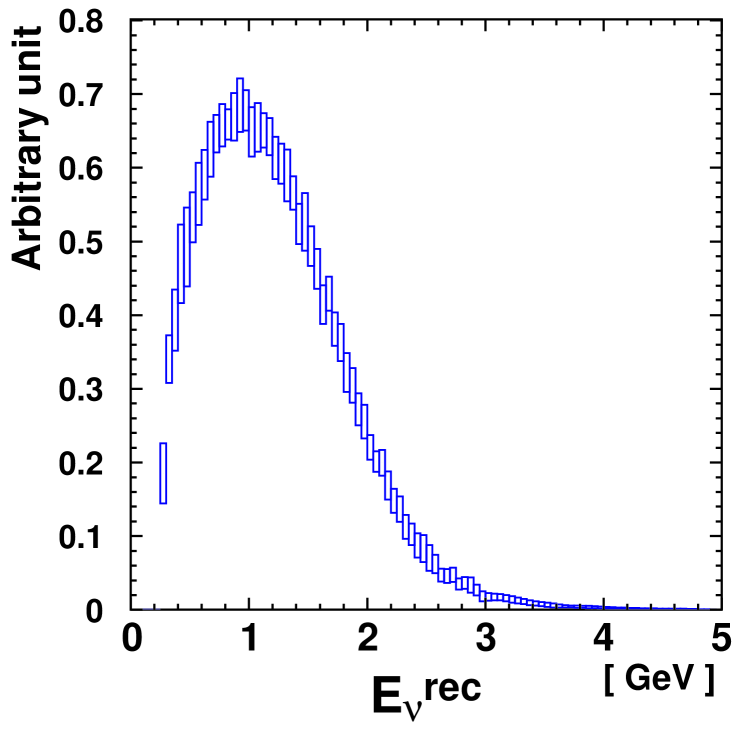
Figure 41: Expected reconstructed neutrino energy spectrum shape in the case of null oscillation. Height of boxes indicate the size of error.

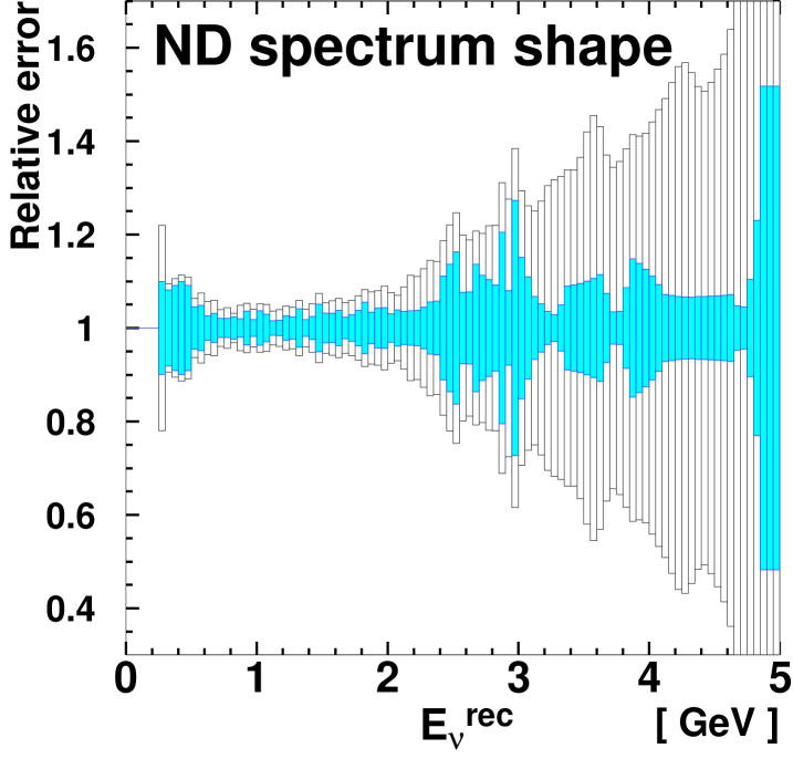
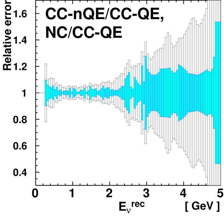
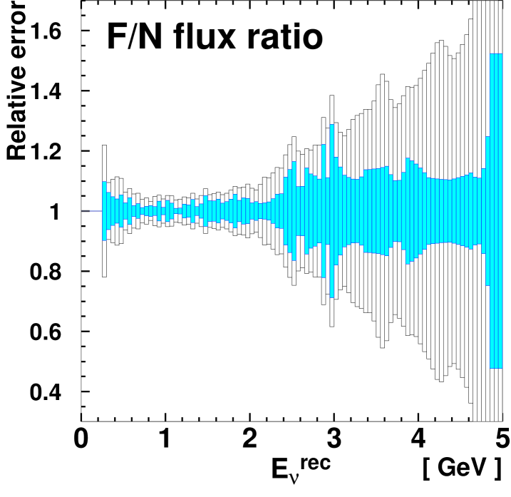
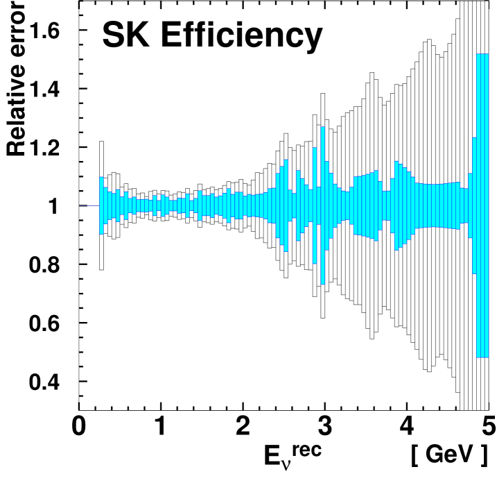
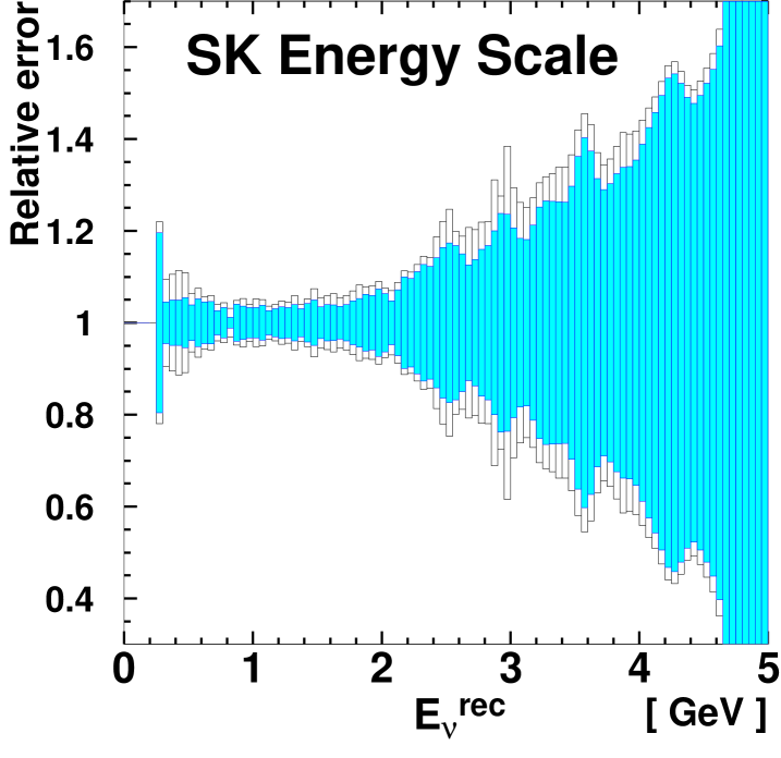
Figure 42: Contribution of each systematic error to the reconstructed neutrino energy spectrum. Vertical axis is relative error of the spectrum. Source of uncertainty is indicated in each plot. Blank and filled bars represent the sizes of the total error and the contribution from the source being considered, respectively.

IX.3 Definition of likelihood

IX.3.1 Normalization term

The normalization term, $\mathcal{L}_{\mathrm{norm}}$, is defined as the Poisson probability to observe $N_{\mathrm{obs}}$ events when the expected number of events is $N_{\mathrm{exp}}$:

$$\mathcal{L}_{\mathrm{norm}}=\frac{(N_{\mathrm{exp}})^{N_{\mathrm{obs}}}}{N_{\mathrm{obs}}!}e^{-N_{\mathrm{exp}}}.$$ (24)

In order to account for the difference of the experimental configuration, the expectation for each experimental period is separately calculated using Eq.(22) and then summed as:

$$N_{\mathrm{exp}}=N_{\mathrm{exp}}^{\mathrm{Ia}}+N_{\mathrm{exp}}^{\mathrm{Ib}}+N_{\mathrm{exp}}^{\mathrm{II}}.$$ (25)

IX.3.2 Energy spectrum shape term

The energy spectrum shape term is defined as the product of the probability for each 1R${\mu}$ event to be observed at reconstructed neutrino energy $E_{\nu}^{\mathrm{rec}}$. We use the expected neutrino energy spectrum, given in Eq. (23), as the probability density function. The probability density function is separately defined for each experimental period:

$$\mathcal{L}_{\mathrm{shape}} = \prod_{i=1}^{N^{\mathrm{Ib}}_{1R{\mu}}}\phi^{\mathrm{SK}}_{\mathrm{exp},\mathrm{Ib}}(E^{\mathrm{rec}}_{\nu,i};\Delta m^{2},\sin^{2}2\theta)$$ (26)

$$\times \prod_{i=1}^{N^{\mathrm{II}}_{1R{\mu}}}\phi^{\mathrm{SK}}_{\mathrm{exp},\mathrm{II}}(E^{\mathrm{rec}}_{\nu,i};\Delta m^{2},\sin^{2}2\theta)$$

where $N^{\mathrm{Ib}}_{1R{\mu}}=30$ and $N^{\mathrm{II}}_{1R{\mu}}=28$ are the number of observed FC 1R${\mu}$ events for period Ib and II, respectively. There is no 1R$\mu$ event in the Ia run period.

IX.3.3 Systematic term

The systematic parameters are treated as fitting parameters, and are assumed to follow a Gaussian distribution. They are constrained within their uncertainties by constraint terms expressed as:

$$\mathcal{L}_{\mathrm{syst}}\equiv\prod_{j=1}^{N_{\mathrm{syst}}}\exp(-{\Delta\mbox{\boldmath$f$}_{j}}^{\mbox{t}}(M_{j})^{-1}\Delta\mbox{\boldmath$f$}_{j}),$$ (27)

where $N_{\mathrm{syst}}$ is the number of parameter sets, $\Delta\mbox{\boldmath$f$}_{j}$ represents the deviations of the parameters from their nominal values and $M_{j}$ is the error matrix for $j$-th set of parameters.

IX.4 Results

The likelihood is maximized in the $\Delta m^{2}$ – $\sin^{2}2\theta$ space and the best fit point within the physical region is found to be at $(\Delta m^{2},\sin^{2}2\theta)=(2.8\times 10^{-3}\mathrm{eV}^{2},1.0)$. The values of all systematic parameters at the best fit point are within 1$\sigma$ of their estimated errors. At this point, the expected number of events is 107.2, which agrees well with the 112 observed within the statistical uncertainty. The observed $E_{\nu}^{\mathrm{rec}}$ distribution is shown in Fig. 43 together with both the expected distributions for the best-fit parameters, and the expectation without oscillations. The consistency between the observed and the best-fit $E_{\nu}^{\mathrm{rec}}$ distributions is checked using a Kolmogorov-Smirnov (KS) test. For the best fit parameters, the KS probability is 37 %, while for the null oscillation hypothesis is 0.07 %. The observation agrees with the expectation of neutrino oscillation. The highest likelihood is found at $(\Delta m^{2},\sin^{2}2\theta)=(2.6\times 10^{-3}\mathrm{eV}^{2},1.2)$, which is outside of the physical region. The probability that we would get $\sin^{2}2\theta\geq 1.2$ if the true parameters are at our best fit point is 26.2%, based on the virtual MC experiments.

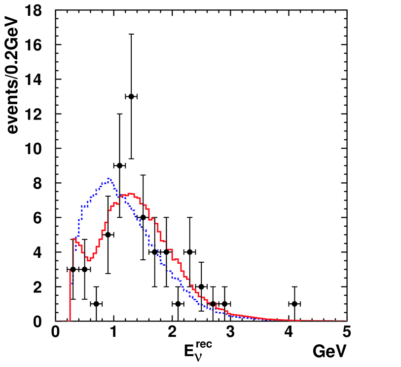
Figure 43: The reconstructed $E_{\nu}$ distribution for the 1-ring $\mu$-like sample. Points with error bars are data. The solid line is the best fit spectrum with neutrino oscillation and the dashed line is the expectation without oscillation. These histograms are normalized by the number of events observed (58).

The probability that the observations can be explained equally well by the no oscillation and by the oscillation hypotheses is estimated by computing the difference of log-likelihood between the null oscillation case and the best fit point with oscillation. The null oscillation probability is calculated to be 0.0015 % (4.3$\sigma$). When only normalization (shape) information is used, the probability is 0.06% (0.42%).

The null oscillation probability calculated separately for each sub-sample or each likelihood term is shown in Tab. 20. In addition, Tab. 21 shows the effect of each systematic uncertainty on the null oscillation probability. The effect is tested by turning on the error source written in the first column in the table. As shown in the table, the dominant contributions to the probabilities for the normalization information are from the $F/N$ flux ratio and the normalization error, while the energy scale is the dominant error source for the probability with the $E_{\nu}^{\mathrm{rec}}$shape information consistent with the results found using the MC test described in Sec. IX.2.2.

Table 20: Summary of the null oscillation probability. Each row is classified by the likelihood term used, and each column represents the data set.

	K2K-I+II	K2K-I only	K2K-II only
Shape + Norm.	0.0015% (4.3$\sigma$)	0.18% ($3.1\sigma$)	0.56% (2.8$\sigma$)
Shape only	0.42% (2.9$\sigma$)	7.7%	5.2%
Norm. only	0.06% (3.4$\sigma$)	0.6%	2.8%

Table 21: Effect of each systematic uncertainty on the null oscillation probability. The numbers in the table are null oscillation probabilities when only the error written in the first column is turned on.

	Norm-only	Shape-only	Combined
Stat. only	0.01%	0.22%	0.0001%
FD spectrum	0.01%	0.24%	0.0002%
nQE/QE, NC/CC	0.01%	0.23%	0.0002%
Far/Near	0.02%	0.23%	0.0003%
$\epsilon^{1R\mu}$	—	0.23%	0.0002%
Energy scale	—	0.38%	0.0002%
Normalization	0.03%	—	0.0005%
All errors	0.06%	0.42%	0.0015%

The allowed region of oscillation parameters are evaluated based on the difference of log-likelihood between each point and the best fit point:

$$\Delta{\ln\mathcal{L}}(\Delta m^{2},\sin^{2}2\theta) \equiv \ln\left(\frac{\mathcal{L}_{\mathrm{max}}^{\mathrm{phys}}}{\mathcal{L}(\Delta m^{2},\sin^{2}2\theta)}\right)$$

$$= \ln\mathcal{L}_{\mathrm{max}}^{\mathrm{phys}}-{\ln\mathcal{L}}(\Delta m^{2},\sin^{2}2\theta),$$

where $\mathcal{L}_{\mathrm{max}}^{\mathrm{phys}}$ is the likelihood at the best-fit point and $\mathcal{L}(\Delta m^{2},\sin^{2}2\theta)$ is the likelihood at $(\Delta m^{2},\sin^{2}2\theta)$ with systematic parameters that maximize the likelihood at that point.

The allowed regions in the neutrino oscillation parameter space, corresponding to the 68%, 90% and 99% confidence levels (CL) are shown in Fig. 44. They are defined as the contour lines with $\ln\mathcal{L}=\ln\mathcal{L}_{\mathrm{max}}^{\mathrm{phys}}-1.37$, $-2.58$ and $-4.91$, respectively. These regions are derived by using the two-dimensional Gaussian approximation from the maximum in the unphysical region Eidelman et al. (2004). The 90% C.L. contour crosses the $\sin^{2}2\theta=1$ axis at $\Delta m^{2}=1.9~{}\mathrm{and}~{}3.5\times 10^{-3}~{}\mathrm{eV}^{2}$. Figure 45 shows the distributions of $\ln\mathcal{L}_{\mathrm{max}}^{\mathrm{phys}}-\ln\mathcal{L}(\Delta m^{2},\sin^{2}2\theta)$ as a function of $\sin^{2}2\theta$ and $\Delta m^{2}$, with a slice at either $\Delta m^{2}=2.8\times 10^{-3}\mathrm{eV}^{2}$ or $\sin^{2}2\theta=1.0$.

We also check the consistency of the fit results performing the analyses with only the normalization term or spectrum shape term, and with the K2K-I or K2K-II sub-samples separately. The fit results are summarized in Tab. 22. There is no entry for the normalization term only, because the two parameters cannot be simultaneously determined from only one number. The oscillation parameters allowed by the normalization and the spectrum shape alone agree with each other, as shown in both Tab. 22 and Fig. 46. The allowed regions calculated with only K2K-I and K2K-II data are also consistent as shown in Tab. 22 and Fig. 47.

Finally, we compare our result with the parameters found by the measurement of atmospheric neutrino oscillation by the Super-Kamiokande collaboration Ashie et al. (2004). Figure 48 shows the allowed regions of oscillation parameters found in this analysis together with the SK result. The K2K result is in good agreement with the parameters found using atmospheric neutrinos, thereby confirming the neutrino oscillation result reported by SK.

Table 22: Summary of the oscillation parameters at the best fit point for each fitting condition.

		All region		Physical region
		$\Delta m^{2}~{}[\mathrm{eV}^{2}]$	$\sin^{2}2\theta$	$\Delta m^{2}~{}[\mathrm{eV}^{2}]$	$\sin^{2}2\theta$
All data	shape + norm.	$2.55\!\times\!10^{-3}$	1.19	$\bf{2.75\!\times\!10^{-3}}$	1.00
	shape only	$2.77\!\times\!10^{-3}$	1.25	$2.95\!\times\!10^{-3}$	1.00
K2K-I	shape + norm.	$2.77\!\times\!10^{-3}$	1.08	$2.89\!\times\!10^{-3}$	1.00
K2K-II	shape + norm.	$2.36\!\times\!10^{-3}$	1.35	$2.64\!\times\!10^{-3}$	1.00

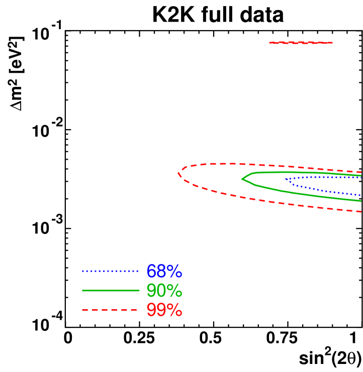
Figure 44: Allowed regions of oscillation parameters. Three contours correspond to the 68% (dotted line), 90% (solid line) and 99% (dashed line) CL. allowed regions, respectively.

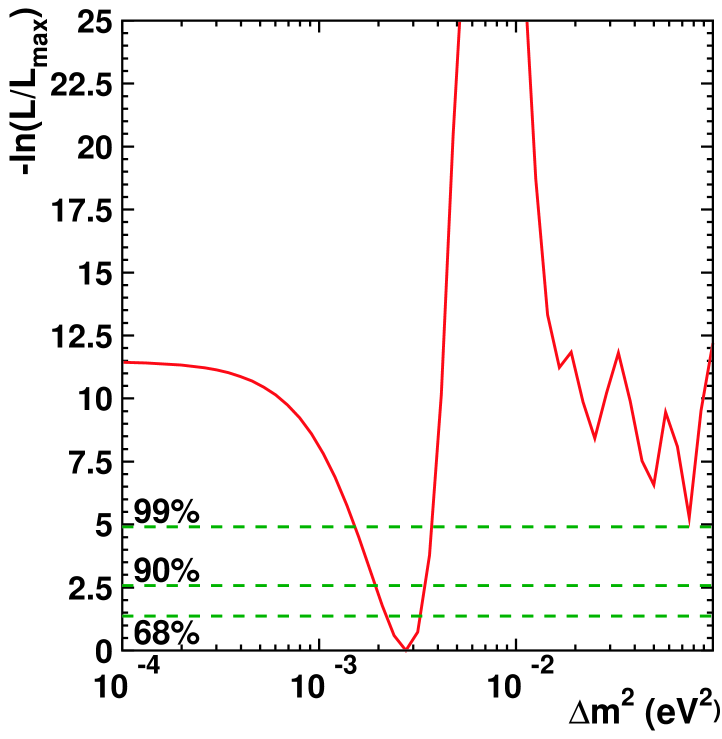
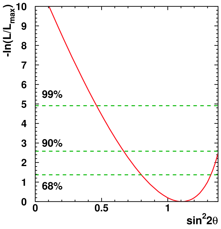
Figure 45: $\ln\mathrm{L}_{\mathrm{max}}^{\mathrm{phys}}-{\ln\mathcal{L}}(\Delta m^{2},\sin^{2}2\theta)$ distribution as a function of $\Delta m^{2}$ (left) and $\sin^{2}2\theta$ (right). $\sin^{2}2\theta$ is set to be 1.0 in the left-hand figure and $\Delta m^{2}$ is set to be $2.8\times 10^{-3}\mathrm{eV}^{2}$ in the right-hand figure. Three horizontal lines correspond to the 68%, 90% and 99% CL interval from the bottom one, respectively.

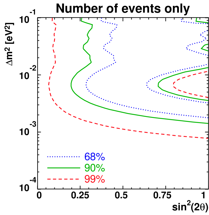
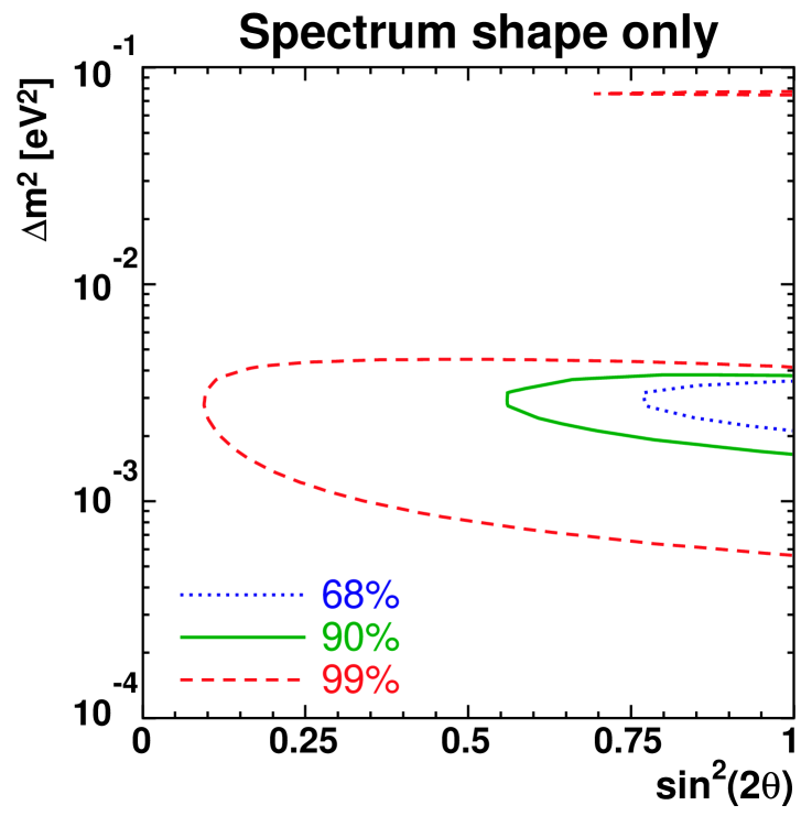
Figure 46: Allowed region of oscillation parameters evaluated with the number of events only (left) and the $E^{\mathrm{rec}}_{\nu}$ spectrum shape only (right). Both information allow the consistent region on the parameters space.

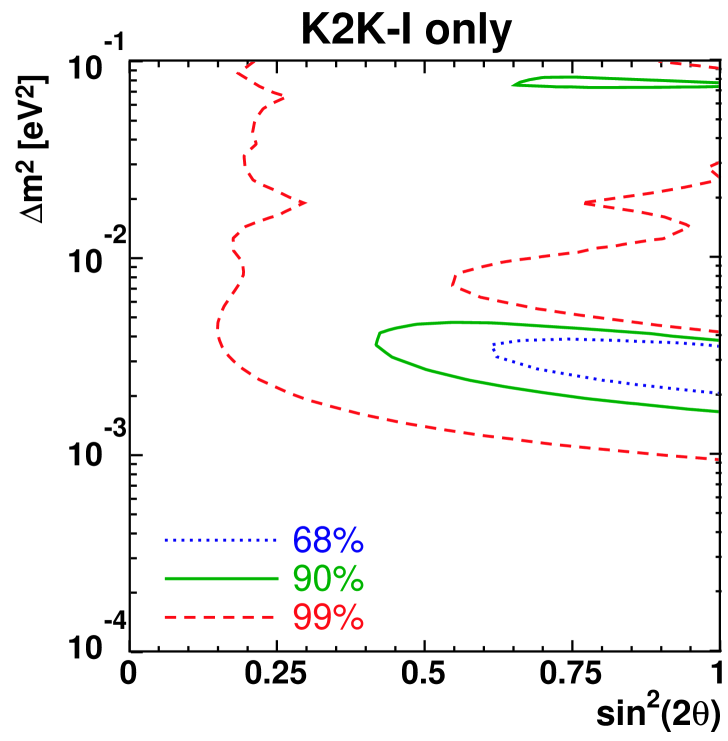
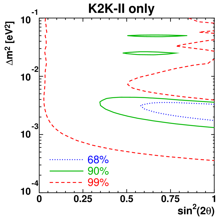
Figure 47: Allowed region of oscillation parameters evaluated with partial data of K2K-I-only (left)/K2K-II-only (right). Both data allow the consistent region on the parameter space.

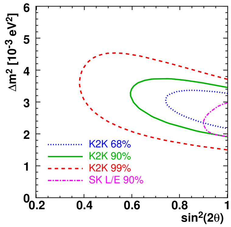
Figure 48: Comparison of K2K results with the SK atmospheric neutrino measurement Ashie et al. (2004). Dotted, solid, dashed and dash-dotted lines represent 68%, 90%, 99% C.L. allowed regions of K2K and 90% C.L. allowed region from SK atmospheric neutrino, respectively.

X Summary

Data taken by the K2K experiment between June 1999 and November 2004 is used to observe and measure the parameters of neutrino oscillation using an accelerator-produced neutrino beam. The K2K experiment is the first long-baseline neutrino experiment to operate at a distance scale of hundreds of kilometers. The neutrinos are measured first by near detectors located approximately 300 meters from the proton target, and then by the Super-Kamiokande detector 250 km away. The near detector complex consists of a 1 kiloton water Cherenkov detector, and a fine grained detector system. The energy spectrum and flux normalization measured at the near detectors are used to predict the signal seen at Super-K. The results found are consistent with the neutrino oscillation parameters previously measured by the Super-Kamiokande collaboration using atmospheric neutrinos.

One hundred and twelve beam-originated neutrino events are observed in the fiducial volume of Super-Kamiokande with an expectation of $158.1^{+9.2}_{-8.6}$ events without oscillation. The spectrum distortion expected from oscillation is also seen in fifty-eight single-ring muon-like events which have had their energy reconstructed. A likelihood analysis was performed and the probability that the observations are explained by a statistical fluctuation with no neutrino oscillation is $0.0015\%$ ($4.3\sigma$). In a two flavor oscillation scenario, the allowed $\Delta m^{2}$ region at $\sin^{2}2\theta=1$ is between $1.9$ and $3.5\times 10^{-3}$ $\rm eV^{2}$ at the 90 % C.L. with a best-fit value of $2.8\times 10^{-3}$ $\rm eV^{2}$.

XI Acknowledgment

We thank the KEK and ICRR directorates for their strong support and encouragement. K2K is made possible by the inventiveness and the diligent efforts of the KEK-PS machine group and beam channel group. We gratefully acknowledge the cooperation of the Kamioka Mining and Smelting Company. This work has been supported by the Ministry of Education, Culture, Sports, Science and Technology of the Government of Japan, the Japan Society for Promotion of Science, the U.S. Department of Energy, the Korea Research Foundation, the Korea Science and Engineering Foundation, NSERC Canada and Canada Foundation for Innovation, the Istituto Nazionale di Fisica Nucleare (Italy), the Ministerio de Educación y Ciencia and Generalitat Valenciana (Spain), the Commissariat à l’Energie Atomique (France), and Polish KBN grants: 1P03B08227 and 1P03B03826.

References

- Ashie et al. (2005) Y. Ashie et al. (Super-Kamiokande), Phys. Rev. D71, 112005 (2005), eprint hep-ex/0501064.
- Ashie et al. (2004) Y. Ashie et al. (Super-Kamiokande), Phys. Rev. Lett. 93, 101801 (2004), eprint hep-ex/0404034.
- Ahn et al. (2003) M. H. Ahn et al. (K2K), Phys. Rev. Lett. 90, 041801 (2003), eprint hep-ex/0212007.
- Aliu et al. (2005) E. Aliu et al. (K2K), Phys. Rev. Lett. 94, 081802 (2005), eprint hep-ex/0411038.
- Ahn et al. (2001) S. H. Ahn et al. (K2K), Phys. Lett. B511, 178 (2001), eprint [http://arXiv.org/abs]hep-ex/0103001.
- Fukuda et al. (2003) Y. Fukuda et al., Nucl. Instrum. Meth. A501, 418 (2003).
- Yamanoi et al. (1997) Y. Yamanoi et al., KEK-preprint 97-225 (1997).
- Yamanoi et al. (1999) Y. Yamanoi et al., KEK-preprint 99-178 (1999), prepared for 16th International Conference on Magnet Technology (MT-16 1999), Tallahassee, Florida, 29 Sep - 1 Oct 1999.
- Kohama (1997) M. Kohama, Master’s thesis, Kobe University (1997), in Japanese.
- Maruyama (2000) T. Maruyama, Ph.D. thesis, Tohoku University (2000).
- Noumi et al. (1997) H. Noumi et al., Nucl. Instrum. Meth. A398, 399 (1997).
- Brun et al. (1987) R. Brun, F. Bruyant, M. Maire, A. C. McPherson, and P. Zanarini (1987), CERN-DD/EE/84-1.
- Sanford and Wang (1967) J. Sanford and C. Wang, AGS Internal Report (unpublished) (1967).
- Wang (1970) C. L. Wang, Phys. Rev. Lett. 25, 1068 (1970).
- Cho et al. (1971) Y. Cho et al., Phys. Rev. D4, 1967 (1971).
- Catanesi et al. (2006) M. G. Catanesi et al. (HARP), Nucl. Phys. B732, 1 (2006), eprint hep-ex/0510039.
- Yamamoto (1981) A. Yamamoto, KEK 81-13 (1981).
- Gabriel et al. (1977) T. A. Gabriel, J. D. Amburgey, and B. L. Bishop (1977), ORNL/TM-5619.
- Zeitnitz and Gabriel (1994) C. Zeitnitz and T. A. Gabriel, Nucl. Instrum. Meth. A349, 106 (1994).
- Fasso et al. (1993) A. Fasso, A. Ferrari, J. Ranft, and P. R. Sala (1993), given at 4th International Conference on Calorimetry in High-energy Physics, La Biodola, Italy, 19-25 Sep 1993.
- Eidelman et al. (2004) S. Eidelman et al. (Particle Data Group), Phys. Lett. B592, 1 (2004).
- Commins and Bucksbaum (1983) E. D. Commins and P. H. Bucksbaum, Weak interactions of leptons and quarks (Cambridge University Press, 1983).
- Suzuki et al. (2000) A. Suzuki et al. (K2K), Nucl. Instrum. Meth. A453, 165 (2000), eprint [http://arXiv.org/abs]hep-ex/0004024.
- Kim et al. (2003) B. J. Kim et al., Nucl. Instrum. Meth. A501, 418 (2003), eprint [http://arXiv.org/abs]hep-ex/0206041.
- Ahn et al. (2000) S. H. Ahn et al., Nucl. Instrum. Meth. A451, 558 (2000).
- Nitta et al. (2004) K. Nitta et al., Nucl. Instrum. Meth. A535, 147 (2004), eprint hep-ex/0406023.
- Pla-Dalmau (2001) A. Pla-Dalmau (MINOS Scintillator Group) (2001), in the proceedings of 9th Conference on Calorimetry in High Energy Physics (CALOR 2000), Annecy, France, 9-14 Oct 2000.
- Yoshida et al. (2004) M. Yoshida et al., IEEE Trans. Nucl. Sci. 51, 3043 (2004).
- Hasegawa (2006) M. Hasegawa, Ph.D. thesis, Kyoto University (2006).
- Buontempo et al. (1994) S. Buontempo et al., Nucl. Instrum. Meth. A349, 70 (1994).
- Glazov et al. (1993) A. Glazov, I. Kisel, E. Konotopskaya, and G. Ososkov, Nucl. Instrum. Meth. A329, 262 (1993).
- Ishii et al. (2002) T. Ishii et al. (K2K MRD Group), Nucl. Instrum. Meth. A482, 244 (2002), eprint [http://arXiv.org/abs]hep-ex/0107041.
- Kawabata et al. (1988) S. Kawabata et al., Nucl. Instrum. Meth. A270, 11 (1988).
- Berns and Wilkes (2000) H. G. Berns and R. J. Wilkes, IEEE Trans. Nucl. Sci. 47, 340 (2000), eprint [http://arXiv.org/abs]hep-ex/9909021.
- Llewellyn Smith (1972) C. H. Llewellyn Smith, Phys. Rept. 3, 261 (1972).
- Smith and Moniz (1972) R. A. Smith and E. J. Moniz, Nucl. Phys. B43, 605 (1972).
- Rein and Sehgal (1981) D. Rein and L. M. Sehgal, Ann. Phys. 133, 79 (1981).
- Rein and Sehgal (1983) D. Rein and L. M. Sehgal, Nucl. Phys. B223, 29 (1983).
- Rein (1987) D. Rein, Z. Phys. C35, 43 (1987).
- Kitagaki et al. (1986) T. Kitagaki et al., Phys. Rev. D34, 2554 (1986).
- Singh et al. (1998) S. K. Singh, M. J. Vicente-Vacas, and E. Oset, Phys. Lett. B416, 23 (1998).
- Hasegawa et al. (2005) M. Hasegawa et al. (K2K), Phys. Rev. Lett. 95, 252301 (2005), eprint hep-ex/0506008.
- Gluck et al. (1995) M. Gluck, E. Reya, and A. Vogt, Z. Phys. C67, 433 (1995).
- Bodek and Yang (2002) A. Bodek and U. K. Yang, Nucl. Phys. Proc. Suppl. 112, 70 (2002), eprint hep-ex/0203009.
- Nakahata et al. (1986) M. Nakahata et al. (KAMIOKANDE), J. Phys. Soc. Jap. 55, 3786 (1986).
- Sjostrand (1994) T. Sjostrand, Comput. Phys. Commun. 82, 74 (1994).
- Barish et al. (1977) S. J. Barish et al., Phys. Rev. D16, 3103 (1977).
- Bonetti et al. (1977) S. Bonetti et al., Nuovo Cim. A38, 260 (1977).
- Ciampolillo et al. (1979) S. Ciampolillo et al. (Gargamelle Neutrino Propane), Phys. Lett. B84, 281 (1979).
- Armenise et al. (1979) N. Armenise et al., Nucl. Phys. B152, 365 (1979).
- Belikov et al. (1985) S. V. Belikov et al., Z. Phys. A320, 625 (1985).
- Radecky et al. (1982) G. M. Radecky et al., Phys. Rev. D25, 1161 (1982).
- Auchincloss et al. (1990) P. S. Auchincloss et al., Z. Phys. C48, 411 (1990).
- Berge et al. (1987) J. P. Berge et al., Z. Phys. C35, 443 (1987).
- Anikeev et al. (1996) V. B. Anikeev et al., Z. Phys. C70, 39 (1996).
- Vovenko et al. (1979) A. S. Vovenko et al., Sov. J. Nucl. Phys. 30, 528 (1979).
- MacFarlane et al. (1984) D. MacFarlane et al., Z. Phys. C26, 1 (1984).
- Baker et al. (1982) N. Baker et al., Phys. Rev. D25, 617 (1982).
- Woods and Saxon (1954) R. Woods and D. Saxon, Phys, Rev. 95, 577 (1954).
- Salcedo et al. (1988) L. L. Salcedo, E. Oset, M. J. Vicente-Vacas, and C. Garcia-Recio, Nucl. Phys. A484, 557 (1988).
- Rowe et al. (1978) G. Rowe, M. Salomon, and R. H. Landau, Phys. Rev. C18, 584 (1978).
- Walter (2002) C. W. Walter, Nucl. Phys. Proc. Suppl. 112, 140 (2002).
- Fesefeldt (1985) H. Fesefeldt (1985), pITHA-85-02.
- Inagaki (2001) T. Inagaki, Ph.D. thesis, Kyoto University (2001).
- Yoshida (2001) M. Yoshida, Ph.D. thesis, Osaka University (2001).
- James and Roos (1975) F. James and M. Roos, Comput. Phys. Commun. 10, 343 (1975).
- Nakayama et al. (2005) S. Nakayama et al. (K2K), Phys. Lett. B619, 255 (2005), eprint hep-ex/0408134.
- Monsay (1978) E. H. Monsay, Phys. Rev. Lett. 41, 728 (1978).