TUM–HEP–404/01

Analytic Approximations for Three Neutrino Oscillation Parameters and Probabilities in Matter

Martin Freund

Theoretische Physik, Physik Department, Technische Universität München,

James–Franck–Strasse, 85748 Garching, Germany

Email: martin.freund@physik.tu-muenchen.de

Abstract

The corrections to neutrino mixing parameters in the presence of matter of constant density are calculated systematically as series expansions in terms of the mass hierarchy ${\Delta m^{2}_{21}}/{\Delta m^{2}_{31}}$. The parameter mapping obtained is then used to find simple, but nevertheless accurate formulas for oscillation probabibilities in matter including CP-effects. Expressions with one to one correspondence to the vacuum case are derived, which are valid for neutrino energies above the solar resonance energy. Two applications are given to show that these results are a useful and powerful tool for analytical studies of neutrino beams passing through the Earth mantle or core: First, the “disentanglement problem” of matter and CP-effects in the CP-asymmetry is discussed and second, estimations of the statistical sensitivity to the CP-terms of the oscillation probabilities in neutrino factory experiments are presented.

1 Introduction

With the development of long baseline neutrino beams passing through the mantle of the Earth, three flavor neutrino oscillation with a constant matter profile is presently drawing attention. Some effort has been spared on the exact solution of the connected cubic eigenvalue problem [1]. However, the obtained solutions are huge and were up to now only used in computer based calculations. Also approximative solutions for oscillation probabilities and mixing angles have been proposed for several parameter regions [2], which are interesting and useful. The intention of this work is to first derive analytic approximations for the mixing parameters in matter according to the standard parameterization, which then allows to compute all desired quantities like probabilities or amplitudes from the known expressions in vacuum by substitution. The parameters in matter are calculated in a series expansion in the small mass hierarchy parameter $\alpha:={\Delta m^{2}_{21}}/{\Delta m^{2}_{31}}$. The obtained results are discussed and then applied to the appearance channel probability $P(\nu_{e}\rightarrow\nu_{\mu})$. A simple solution, which is easy to use, but nevertheless accurate over a wide parameter range is obtained. No new notation is introduced besides abbreviations known from two neutrino oscillation in matter. Furthermore, the result shows at first sight the convergence to the vacuum case at small baselines and thus is directly connected to the terms in vacuum. The approximate solutions obtained with this method are a powerful tool for further analytical studies. To demonstrate this, two applications are given. First the derived expressions are exploited to compute the frequently used quantity called the CP-asymmetry $A^{\mathrm{CP}}$, which has considerable importance in CP-violation studies. The problem is that matter effects cause contributions to the CP-asymmetry, which cannot easily be distinguished from intrinsic CP-effects. Here, expressions for $A^{\mathrm{CP}}$ in matter are given for high neutrino energies (more precise: low $L/E_{\nu}$). The result is then used to investigate what can be learned from the energy dependence of $A^{\mathrm{CP}}$. The second application given estimates the statistical sensitivity to the CP-terms of the oscillation probabilities in neutrino factory long baseline experiments. Plots are presented, which show the magnitude of CP-effects at different baselines and beam energies. Contrarily to what presently can be found in the literature, the here obtained results indicate strongly that, in general, the low energy option is not the best solution to measure effects from the CP-phase $\delta$. The reason for this discrepancy is discussed.

Throughout this work two assumptions will be made: First, that the mass hierarchy parameter $\alpha:={\Delta m^{2}_{12}}/{\Delta m^{2}_{31}}$, which is used as expansion parameter, is small. Consider for example an atmospheric ${\Delta m^{2}}$ of $3.2\cdot 10^{-3}\,\mathrm{eV}^{2}$ [3] . For solar mass differences of LMA-scale [4] between $10^{-5}\,\mathrm{eV}^{2}$ and $10^{-4}\,\mathrm{eV}^{2}$, $\alpha$ varies between 0.0031 and 0.031. Second, it will be assumed that the mixing angle $\theta_{13}$ is small as indicated by reactor, solar, and atmospheric experiments. The strongest bound is given by the CHOOZ experiment [5] with $\sin^{2}2\theta_{13}<0.1$. The smallness of this parameter will be used to classify terms, which appear in the expressions for oscillation probabilities. The mixing angles $\theta_{12}$ and $\theta_{23}$ should be chosen from the interval $[0,\pi/2]$.

2 Three neutrino oscillation in vacuum

In vacuum, the neutrino oscillation probabilities are given by the well-known formulas

$$P(\nu_{e_{l}}\rightarrow\nu_{e_{m}})=\delta_{lm}-4\sum_{i>j}\mathrm{Re}J_{ij}^{lm}\sin^{2}\hat{\Delta}_{ij}-2\sum_{i>j}\mathrm{Im}J_{ij}^{lm}\sin 2\hat{\Delta}_{ij}~{},$$ (1)

with the abbreviations $J_{ij}^{lm}:=U_{li}U_{lj}^{*}U^{*}_{mi}U_{mj}$ and $\hat{\Delta}_{ij}:=\Delta m^{2}_{ij}L/(4E)$. Here, $U$ is the mixing matrix of the neutrino sector in standard parameterization form:

$$U=\left(\begin{array}[]{ccc}c_{12}c_{13}&c_{13}s_{12}&e^{-i\delta}s_{13}\\ -s_{12}c_{23}-e^{i\delta}c_{12}s_{13}s_{23}&c_{12}c_{23}-e^{i\delta}s_{12}s_{13}s_{23}&c_{13}s_{23}\\ -e^{i\delta}c_{12}s_{13}c_{23}+s_{12}s_{23}&-e^{i\delta}s_{12}s_{13}c_{23}-c_{12}s_{23}&c_{13}c_{23}\end{array}\right)~{}.$$ (2)

Since in this work, the hierarchy $|{\Delta m^{2}_{21}}|\ll|{\Delta m^{2}_{31}}|$ between the two mass squared differences is exploited, from now on all mass squared differences will always be related to the atmospheric squared mass difference: ${\Delta m^{2}_{31}}=:\Delta$, ${\Delta m^{2}_{21}}=\alpha\Delta$, ${\Delta m^{2}_{32}}=(1-\alpha)\Delta$, and $\hat{\Delta}=\Delta L/(4E)$. Series expansion up to order $\alpha^{2}$ gives the following important terms in the oscillation probability $P(\nu_{e}\rightarrow\nu_{\mu})\approx P_{0}+P_{\sin\delta}+P_{\cos\delta}+P_{3}$:

$$P_{0} = \sin^{2}\theta_{23}\sin^{2}2\theta_{13}\sin^{2}\hat{\Delta}$$ (3a)

$$P_{\sin\delta} = \alpha\;\sin\delta\cos\theta_{13}\sin 2\theta_{12}\sin 2\theta_{13}\sin 2\theta_{23}\sin^{3}\hat{\Delta}$$ (3b)

$$P_{\cos\delta} = \alpha\;\cos\delta\cos\theta_{13}\sin 2\theta_{12}\sin 2\theta_{13}\sin 2\theta_{23}\cos\hat{\Delta}\sin^{2}\hat{\Delta}$$ (3c)

$$P_{3} = \alpha^{2}\cos^{2}\theta_{23}\sin^{2}2\theta_{12}\sin^{2}\hat{\Delta}$$ (3d)

Expanding the oscillatory terms in $\alpha$ means linearization of the oscillation over the solar mass squared difference. This gives valid results only for $\alpha\hat{\Delta}\lesssim 1$. With todays knowledge about neutrino masses this does not cause crucial errors for neutrino energies above 1 GeV at baselines below approximately 10000 km. The two terms $P_{\sin\delta}$ and $P_{\cos\delta}$, containing the CP-phase $\delta$, are both of order $\alpha$ and hence suppressed by the mass hierarchy. This reflects the fact that CP-effects vanish when the mass hierarchy becomes large. Besides the factor $\sin^{2}\theta_{23}$, the term $P_{0}$ is similar to the two neutrino oscillation probability which in matter is expected to show the resonant behavior called MSW-effect [6]. The term $P_{3}$ is the only term of order $\alpha^{2}$, which is not suppressed by the small mixing angle $\theta_{13}$. Hence, it is important to take this term into account when $\theta_{13}$ is small. If $\theta_{13}$ is not too far away from the CHOOZ-bound, $P_{3}$ can safely be neglected. All other terms of order $\alpha^{2}$ are additionally suppressed by one or more powers of $\theta_{13}$ and are not listed here.

3 Mixing parameters in matter

In matter, the effective Hamiltonian in flavor basis is given by

$$\mathcal{H}=\frac{1}{2E}\left[U\left(\begin{array}[]{ccc}m_{1}^{2}&0&0\\ 0&m_{2}^{2}&0\\ 0&0&m_{3}^{2}\end{array}\right)U^{\dagger}+\left(\begin{array}[]{ccc}A&0&0\\ 0&0&0\\ 0&0&0\end{array}\right)\right]~{}.$$ (4)

Here $U=U_{23}(\theta_{23})U_{13}(\theta_{13},\delta)U_{12}(\theta_{12})$ is the mixing matrix, which rotates from mass to flavor basis. The second term is generated by matter effects with $A=2VE_{\nu}$ and $V=\sqrt{2}G_{F}n_{e}$, where $G_{F}$ is the Fermi coupling constant and $n_{e}$ is the electron density of the matter, which is crossed by the neutrino beam.

The matter term is invariant under rotations in the 23-subspace. Separating $\mathrm{diag}(m_{1}^{2},m_{1}^{2},m_{1}^{2})$ which, as global phase, does not contribute to the probability, and using the above defined parameters, the Hamiltonian can be written in the form

$$\mathcal{H}=\frac{\Delta}{2E}U_{23}\left[U_{13}U_{12}\left(\begin{array}[]{ccc}0&0&0\\ 0&\alpha&0\\ 0&0&1\end{array}\right)U_{12}^{\dagger}U_{13}^{\dagger}+\left(\begin{array}[]{ccc}\frac{A}{\Delta}&0&0\\ 0&0&0\\ 0&0&0\end{array}\right)\right]U_{23}^{\dagger}~{}.$$ (5)

With

$$U_{\delta}:=\left(\begin{array}[]{ccc}1&0&0\\ 0&1&0\\ 0&0&e^{i\delta}\end{array}\right)~{},$$ (6)

the relations

$$U_{\delta}^{\dagger}\,U_{13}(\theta_{13},\delta)\,U_{\delta} = U_{13}(\theta_{13},0)~{},$$ (7a)

$$U_{\delta}^{\dagger}\,U_{12}(\theta_{12})\,U_{\delta} = U_{12}(\theta_{12})~{},$$ (7b)

$$U_{\delta}^{\dagger}\,\mathrm{diag}(a,b,c)\,U_{\delta} = \mathrm{diag}(a,b,c)$$ (7c)

are valid. Inserting the identity matrix $U_{\delta}\,U_{\delta}^{\dagger}$ at the appropriate places in eq. (5) gives

$$\mathcal{H}=\frac{\Delta}{2E}U_{23}\,U_{\delta}\underbrace{\left[U_{13}(\theta_{13},0)\,U_{12}\left(\begin{array}[]{ccc}0&0&0\\ 0&\alpha&0\\ 0&0&1\end{array}\right)U_{12}^{\dagger}\,U_{13}(\theta_{13},0)^{\dagger}+\left(\begin{array}[]{ccc}\frac{A}{\Delta}&0&0\\ 0&0&0\\ 0&0&0\end{array}\right)\right]}_{M}U_{\delta}^{\dagger}\,U_{23}^{\dagger}~{}.$$ (8)

Diagonalization of the real matrix $M$ by $\hat{U}:=U_{23}(\hat{\theta}_{23})\,U_{13}(\hat{\theta}_{13})\,U_{12}(\hat{\theta}_{12})$ together with the part which was factored out gives the complete mixing matrix $U^{\prime}$ in matter:

$$U^{\prime}=U_{23}(\theta_{23})\,U_{\delta}\,U_{23}(\hat{\theta}_{23})\,U_{13}(\hat{\theta}_{13})\,U_{12}(\hat{\theta}_{12})~{}.$$ (9)

Mixing angles in standard parameterization form

The matrix $U^{\prime}$ must still be brought to the standard form. The matrix

$$U_{23}(\theta_{23})\,U_{\delta}\,U_{23}(\hat{\theta}_{23})=\left(\begin{array}[]{ccc}1&0&0\\ 0&C&S\\ 0&-e^{i\delta}S^{*}&e^{i\delta}C^{*}\end{array}\right)$$ (10)

with

$$C := \cos\theta_{23}\cos\hat{\theta}_{23}-e^{i\delta}\sin\theta_{23}\sin\hat{\theta}_{23}~{},$$ (11a)

$$S := \cos\theta_{23}\sin\hat{\theta}_{23}+e^{i\delta}\sin\theta_{23}\cos\hat{\theta}_{23}$$ (11b)

can be made real by the phase rotations $\beta:=-\mathrm{arg}\,C$, $\gamma:=\mathrm{arg}\,S$, and $\delta^{\prime}:=\mathrm{arg}\,C-\mathrm{arg}\,S$ :

$$\left(\begin{array}[]{ccc}1&0&0\\ 0&e^{-i\beta}&0\\ 0&0&-e^{(i\delta-\gamma)}\end{array}\right)\,U_{23}(\theta_{23})\,U_{\delta}\,U_{23}(\hat{\theta}_{23})\,\left(\begin{array}[]{ccc}1&0&0\\ 0&1&0\\ 0&0&e^{-i\delta^{\prime}}\end{array}\right)=\left(\begin{array}[]{ccc}1&0&0\\ 0&|C|&|S|\\ 0&-|S|&|C|\end{array}\right)~{}.$$ (12)

This gives

$$U^{\prime}=\left(\begin{array}[]{ccc}1&0&0\\ 0&e^{i\beta}&0\\ 0&0&-e^{(i\gamma-\delta)}\end{array}\right)\,\left(\begin{array}[]{ccc}1&0&0\\ 0&|C|&|S|\\ 0&-|S|&|C|\end{array}\right)\,U_{\delta^{\prime}}\,U_{13}(\hat{\theta}_{13})\,U^{\dagger}_{\delta^{\prime}}\,U_{12}(\hat{\theta}_{12})\,U_{\delta^{\prime}}~{}.$$ (13)

The phase rotations on the left and on the right can be absorbed in the field vectors, yielding then $U^{\prime}$ in standard parameterization form:

$$U^{\prime}=U(\theta_{23}^{\prime})\,U_{13}(\hat{\theta}_{13},\delta^{\prime})\,U_{12}(\hat{\theta}_{12})~{}.$$ (14)

This finally means, that the (standard) mixing angles $\theta_{13}^{\prime}$ and $\theta_{12}^{\prime}$ in matter are equal to $\hat{\theta}_{13}$ and $\hat{\theta}_{12}$ which are obtained from the matrix that diagonalizes $M$. The matter correction $\hat{\theta}_{23}$, however, mixes with the CP-phase $\delta$:

$$\theta_{13}^{\prime} = \hat{\theta}_{13}~{},$$ (15a)

$$\theta_{12}^{\prime} = \hat{\theta}_{12}~{},$$ (15b)

$$\sin^{2}\theta_{23}^{\prime} = \cos^{2}\theta_{23}\sin^{2}\hat{\theta}_{23}+\sin^{2}\theta_{23}\cos^{2}\hat{\theta}_{23}+2\cos\delta\sin\theta_{23}\cos\theta_{23}\sin\hat{\theta}_{23}\cos\hat{\theta}_{23}~{},$$ (15c)

$$\sin\delta^{\prime} = \sin\delta\,\frac{\sin 2\theta_{23}}{\sin 2\theta_{23}^{\prime}}~{}.$$ (15d)

Equation (15d) was first found by S. Toshev [7]. There, a different parameterization is used, which – for oscillations – is equivalent to the standard parameterization. It is important to note that the results given up to here are exact results for three neutrino oscillation in matter and do not presume that the mass hierarchy parameter is small.

Calculation of the eigenvalues and eigenvectors

Hereafter $\hat{A}$ will be used as abbreviation for $\frac{A}{\Delta}$. Diagonalization of the matrix $M$ leads to the oscillation parameters in matter. Note that $M$ does not include the parameters $\theta_{23}$ and $\delta$, which have been factored out. This will simplify the calculation of the eigenvalues and eigenvectors of $M$ considerably:

$$M=\left(\begin{array}[]{ccc}s^{2}_{13}+\hat{A}+\alpha c^{2}_{13}s^{2}_{12}&\alpha s_{12}c_{12}c_{13}&s_{13}c_{13}-\alpha s_{13}c_{13}s^{2}_{12}\\ \alpha s_{12}c_{12}c_{13}&\alpha c^{2}_{12}&-\alpha s_{12}c_{12}s_{13}\\ s_{13}c_{13}-\alpha s_{13}c_{13}s^{2}_{12}&-\alpha s_{12}c_{12}s_{13}&c^{2}_{13}+\alpha s^{2}_{12}s^{2}_{13}\end{array}\right)~{}.$$ (16)

The invariants of the cubic eigenvalue problem are given by

$$I_{1} = \mathrm{Tr}(M)=\lambda_{1}+\lambda_{2}+\lambda_{3}=$$ (17a)

$$= \hat{A}+1+\alpha~{},$$

$$I_{2} = \frac{1}{2}\left[\mathrm{Tr}(M)-\mathrm{Tr}(M^{2})\right]=\lambda_{1}\lambda_{2}+\lambda_{1}\lambda_{3}+\lambda_{2}\lambda_{3}=$$ (17b)

$$= \hat{A}\cos^{2}\theta_{13}+\alpha+\alpha\hat{A}\left(\sin^{2}\theta_{13}\sin^{2}\theta_{12}+\cos^{2}\theta_{12}\right)~{},$$

$$I_{3} = \mathrm{Det}(M)=\lambda_{1}\lambda_{2}\lambda_{3}=$$ (17c)

$$= \alpha\hat{A}\cos^{2}\theta_{13}\cos^{2}\theta_{12}~{}.\$$

Solving this system of equations in a series expansion of $\alpha$ gives the eigenvalues

$$\lambda_{1} = \frac{1}{2}(\hat{A}+1-\hat{C})+\alpha\;\frac{(\hat{C}+1-\hat{A}\cos 2\theta_{13})\sin^{2}\theta_{12}}{2\hat{C}}+\mathcal{O}(\alpha^{2})~{},$$ (18a)

$$\lambda_{2} = \alpha\cos^{2}\theta_{12}+\mathcal{O}(\alpha^{2})~{},$$ (18b)

$$\lambda_{3} = \frac{1}{2}(\hat{A}+1+\hat{C})+\alpha\;\frac{(\hat{C}-1+\hat{A}\cos 2\theta_{13})\sin^{2}\theta_{12}}{2\hat{C}}+\mathcal{O}(\alpha^{2})~{},$$ (18c)

with

$$\hat{C}=\sqrt{(\hat{A}-\cos 2\theta_{13})^{2}+\sin^{2}2\theta_{13}}~{}.$$ (19)

Here, $\hat{C}$ is the same square root, which appears in the two neutrino matter formulas.

Calculating the eigenvectors of $M$ in order $\mathcal{O}(\alpha)$ gives:

$$v_{1} = \left(\begin{array}[]{c}\frac{\sin 2\theta_{13}}{\sqrt{2\hat{C}(\hat{A}+\hat{C}-\cos 2\theta_{13})}}-\frac{\alpha\;\hat{A}\sin^{2}\theta_{12}\sin^{2}2\theta_{13}}{2\hat{C}\sqrt{2\hat{C}^{2}(-\hat{A}+\hat{C}+\cos 2\theta_{13})}}\\ \frac{\alpha\;(1+\hat{A}-\hat{C})\sin 2\theta_{12}\sin\theta_{13}}{(1+\hat{A}+\hat{C})\sqrt{2\hat{C}(\hat{A}+\hat{C}-\cos 2\theta_{13})}}\\ -\frac{\sin 2\theta_{13}}{\sqrt{2\hat{C}(-\hat{A}+\hat{C}+\cos 2\theta_{13})}}-\frac{\alpha\;\hat{A}\sin^{2}\theta_{12}\sin^{2}2\theta_{13}}{2\hat{C}\sqrt{2\hat{C}^{2}(\hat{A}+\hat{C}-\cos 2\theta_{13})}}\end{array}\right)+\mathcal{O}(\alpha^{2})~{},$$ (20d)

$$v_{2} = \left(\begin{array}[]{c}-\frac{\alpha\;\cos\theta_{12}\sin\theta_{12}}{\hat{A}\cos\theta_{13}}\\ 1\\ \frac{\alpha\;(1+\hat{A})\cos\theta_{12}\sin\theta_{12}\sin\theta_{13}}{\hat{A}\cos^{2}\theta_{13}}\end{array}\right)+\mathcal{O}(\alpha^{2})~{},$$ (20h)

$$v_{3} = \left(\begin{array}[]{c}\frac{\sin 2\theta_{13}}{\sqrt{2\hat{C}(-\hat{A}+\hat{C}+\cos 2\theta_{13})}}+\frac{\alpha\;\hat{A}\sin^{2}\theta_{12}\sin^{2}2\theta_{13}}{2\hat{C}\sqrt{2\hat{C}^{2}(\hat{A}+\hat{C}-\cos 2\theta_{13})}}\\ \frac{\alpha\;(1+\hat{A}-\hat{C})\sin 2\theta_{12}\sin\theta_{13}}{(1+\hat{A}+\hat{C})\sqrt{2\hat{C}(-\hat{A}+\hat{C}+\cos 2\theta_{13})}}\\ \frac{\sin 2\theta_{13}}{\sqrt{2\hat{C}(\hat{A}+\hat{C}-\cos 2\theta_{13})}}-\frac{\alpha\;\hat{A}\sin^{2}\theta_{12}\sin^{2}2\theta_{13}}{2\hat{C}\sqrt{2\hat{C}^{2}(-\hat{A}+\hat{C}+\cos 2\theta_{13})}}\end{array}\right)+\mathcal{O}(\alpha^{2})~{}.$$ (20l)

There is one major problem concerning the calculation of the eigenvalues and eigenvectors, which has to be addressed. Throughout the above series expansion $\hat{A}$ was assumed to be different from zero. This is important as the results given above do not hold for $\hat{A}=0$ in which case a different series expansion in $\alpha$ would be obtained. This is a general and important fact. In principle, it is also possible to give results for small values of $|\hat{A}|$, which, however, would fail for larger $|\hat{A}|$. The reason for this is that there are two different resonances occurring. One for $\hat{A}=\alpha$ (solar resonance) and one for $\hat{A}=\cos 2\theta_{13}$ (atmospheric resonance). Each resonance produces a level-crossing of the eigenvalues. To describe both level-crossings, the correct expression for the eigenvalues are necessary. Being interested in approximative solutions, one has to distinguish the two above mentioned cases. In this work the focus is on the case $|\hat{A}|>\alpha$, which is appropriate for neutrino beams above 1 GeV in matter densities of $2.8~{}\mathrm{g}/\mathrm{cm}^{3}$ (Earth mantle) or more. However, one must not expect that the expressions for the mixing parameters in matter will show the correct convergence for $\hat{A}\rightarrow 0$. For ${\Delta m^{2}_{21}}=10^{-4}\,\mathrm{eV}^{2}$ and $2.8~{}\mathrm{g}/\mathrm{cm}^{3}$ we find that $\hat{A}>\alpha$ is valid for $E_{\nu}>0.5\,\mathrm{GeV}$. This lower bound on the neutrino energy decreases linearly with ${\Delta m^{2}_{21}}$.

That the results for the eigenvalues and eigenvectors obtained from the series expansion are not good at the resonance $\hat{A}\approx 1$ is another point to mention. However, this does not have a crucial implication on the obtained results for the parameter mapping and oscillation probabilities. This issue will be discussed later, at the appropriate places.

Construction of $\hat{U}$

It is now possible to construct $\hat{U}$ from the eigenvectors $v_{1}$, $v_{2}$, and $v_{3}$. For this it is necessary to correctly identify the order and the signs of the eigenvectors. In order to avoid divergences in the expressions for the mixing angles, it is appropriate to change the order at the resonance $\hat{A}=\cos 2\theta_{13}$ :

$$\hat{U}=\left\{\begin{array}[]{crl}\left(v_{1}\,v_{2}\,v_{3}\right)^{T}&\mathrm{for}&\qquad\hat{A}<\cos 2\theta_{13}\\ \left(v_{3}\,v_{2}\,v_{1}\right)^{T}&\mathrm{for}&\qquad\hat{A}>\cos 2\theta_{13}\end{array}\right.~{}.$$ (21)

The second point is to bring $U^{\prime}$ to a form which is consistent with the standard parameterization. This is not trivial and has to be carried out carefully for each of the different cases. As an example, the case $\hat{A}<0$ will be considered in detail:

As the vacuum angle $\theta_{23}$ was factored out from the beginning (eq. (8)), the matter induced change of this mixing angle $\hat{\theta}_{23}$ will be of order $\alpha$. This can be also seen by looking at the ($\mu,3$)-element of $\hat{U}$. Furthermore, by looking at the $(e,2)$-element, one finds that also $\hat{\theta}_{12}$ must be of order $\alpha$. Considering this with the replacements $\hat{s}_{12}=\alpha\hat{s}_{12}^{(\alpha)}$, $\hat{s}_{23}=\alpha\hat{s}_{23}^{(\alpha)}$, and $\hat{s}_{13}=\hat{s}_{13}^{(0)}+\alpha\hat{s}_{13}^{(\alpha)}$, one obtains the following structure for $\hat{U}$:

$$\hat{U}=\left(\begin{array}[]{ccc}\hat{c}_{13}&\alpha\hat{c}_{13}^{(0)}\hat{s}_{12}^{(\alpha)}&\hat{s}_{13}\\ -\alpha(\hat{s}_{12}^{(\alpha)}+\hat{s}_{13}^{(0)}\hat{s}_{23}^{(\alpha)})&1&\alpha\hat{c}_{13}^{(0)}\hat{s}_{23}^{(\alpha)}\\ -\hat{s}_{13}&-\alpha(\hat{s}_{12}^{(\alpha)}\hat{s}_{13}^{(0)}+\hat{s}_{23}^{(\alpha)})&\hat{c}_{13}\end{array}\right)+\mathcal{O}(\alpha^{2})~{}.$$ (22)

Then, $\sin\hat{\theta}_{13}$ and $\sin\hat{\theta}_{23}$ can be read off directly from $\hat{U}_{e3}$, $\hat{U}_{\mu 3}$ and $\hat{U}_{\tau 3}$:

$$\sin\hat{\theta}_{13} = \frac{\sin 2\theta_{13}}{\sqrt{2\hat{C}(-\hat{A}+\hat{C}+\cos 2\theta_{13})}}+\frac{\alpha\;\hat{A}\sin^{2}\theta_{12}\sin^{2}2\theta_{13}}{2\hat{C}\sqrt{2\hat{C}^{2}(\hat{A}+\hat{C}-\cos 2\theta_{13})}}+\mathcal{O}(\alpha^{2})~{},$$ (23)

$$\sin\hat{\theta}_{23} = \alpha\frac{(1+\hat{A}-\hat{C})\sin 2\theta_{12}\sin\theta_{13}}{2(1-\hat{A}+\hat{C})\cos^{2}\theta_{13}}+\mathcal{O}(\alpha^{2})~{}.$$ (24)

To find $\sin\hat{\theta}_{12}$, it is now useful to split off $\hat{\theta}_{23}$. The rest $\hat{U}=U_{23}^{T}(\hat{\theta}_{23})\,\hat{U}^{\prime}$ should now be brought to the form

$$\left(\begin{array}[]{ccc}\hat{c}_{13}&\alpha\hat{c}_{13}^{(0)}\hat{s}_{12}^{(\alpha)}&\hat{s}_{13}\\ -\alpha\hat{s}_{12}^{(\alpha)}&1&0\\ -\hat{s}_{13}^{\prime}&-\alpha\hat{s}_{12}^{(\alpha)}\hat{s}_{13}^{(0)}&\hat{c}_{13}\end{array}\right)+\mathcal{O}(\alpha^{2})~{}.$$ (25)

The mixing angle $\hat{\theta}_{12}$ can then be read off from $\hat{U}^{\prime}_{\mu 1}$:

$$\sin\hat{\theta}_{12}=-\frac{\alpha\;\hat{C}\sin 2\theta_{12}}{\hat{A}\cos\theta_{13}\sqrt{2\hat{C}(-\hat{A}+\hat{C}+\cos 2\theta_{13})}}+\mathcal{O}(\alpha^{2})~{}.$$ (26)

Parameter mapping

Considering the correct ordering of the eigenvectors (eq. (21)) and following the above described steps, one can determine the complete parameter mapping for all regions of the $\hat{A}$ parameter space. Comprising, one obtains the following expressions for the mixing parameters in matter:

$$\sin\theta^{\prime}_{13} = \frac{\sin 2\theta_{13}}{\sqrt{2\hat{C}(\mp\hat{A}+\hat{C}\pm\cos 2\theta_{13})}}\pm\frac{\alpha\;\hat{A}\sin^{2}\theta_{12}\sin^{2}2\theta_{13}}{2\hat{C}^{2}\sqrt{2\hat{C}(\pm\hat{A}+\hat{C}\mp\cos 2\theta_{13})}}$$ (27a)

$$\sin\theta^{\prime}_{12} = \alpha\;\frac{\hat{C}\sin 2\theta_{12}}{|\hat{A}|\cos\theta_{13}\sqrt{2\hat{C}(\mp\hat{A}+\hat{C}\pm\cos 2\theta_{13})}}$$ (27b)

$$\sin\theta^{\prime}_{23} = \sin\theta_{23}+\alpha\,\cos\delta\;\frac{\hat{A}\sin 2\theta_{12}\sin\theta_{13}\cos{\theta_{23}}}{\pm 1+\hat{C}\mp\hat{A}\cos 2\theta_{13}}$$ (27c)

$$\sin\delta^{\prime} = \sin\delta\left(1-\alpha\,\frac{\cos\delta}{\tan 2\theta_{23}}\;\frac{2\hat{A}\sin 2\theta_{12}\sin\theta_{13}}{\pm 1+\hat{C}\mp\hat{A}\cos 2\theta_{13}}\right)$$ (27d)

Here, in the expressions with choices for the sign, the upper sign holds for $\hat{A}<\cos 2\theta_{13}$ and the lower sign holds for $\hat{A}>\cos 2\theta_{13}$. Higher orders than $\mathcal{O}(\alpha)$ are omitted. To take into account also $\theta_{23}$ and $\delta$, which were factored out at the beginning, the equations (15a-d) were applied. The expansion of $\sin\delta^{\prime}$ given here does not hold for $\theta_{23}\rightarrow 0$.

From this parameter mapping it is possible to derive the following quantities:

$$\sin^{2}2\theta^{\prime}_{13} = \frac{\sin^{2}2\theta_{13}}{\hat{C}^{2}}+\alpha\;\frac{2\hat{A}(-\hat{A}+\cos 2\theta_{13})\sin^{2}\theta_{12}\sin^{2}2\theta_{13}}{\hat{C}^{4}}$$ (28a)

$$\sin 2\theta^{\prime}_{12} = \alpha\;\frac{2\hat{C}\sin 2\theta_{12}}{|\hat{A}|\cos\theta_{13}\sqrt{2\hat{C}(\mp\hat{A}+\hat{C}\pm\cos 2\theta_{13})}}$$ (28b)

$$\sin 2\theta^{\prime}_{23} = \sin 2\theta_{23}+\alpha\cos\delta\;\frac{2\hat{A}\sin 2\theta_{12}\sin\theta_{13}\cos 2\theta_{23}}{\pm 1+\hat{C}\mp\hat{A}\cos 2\theta_{13}}$$ (28c)

For the mass squared differences one obtains:

$$({\Delta m^{2}_{21}}^{\prime},{\Delta m^{2}_{31}}^{\prime},{\Delta m^{2}_{32}}^{\prime})=\left\{\begin{array}[]{ll}(\;\;\;\Delta m^{2}_{3},\;\;\;\Delta m^{2}_{2},\;\;\;\Delta m^{2}_{1})&\mathrm{for}\quad\hat{A}<\cos 2\theta_{13}\\ (-\Delta m^{2}_{1},-\Delta m^{2}_{2},-\Delta m^{2}_{3})&\mathrm{for}\quad\hat{A}>\cos 2\theta_{13}\end{array}\right.$$ (29)

with

$${\Delta m^{2}_{1}}^{\prime} := \Delta(\lambda_{3}-\lambda_{2})$$ (30a)

$$= \frac{1}{2}(1+\hat{A}+\hat{C})\Delta-\alpha\Delta\left(\cos^{2}\theta_{12}-\frac{(-1+\hat{C}+\hat{A}\cos 2\theta_{13})\sin^{2}\theta_{12}}{2\hat{C}}\right)~{},$$

$${\Delta m^{2}_{3}}^{\prime} := \Delta(\lambda_{2}-\lambda_{1})$$ (30b)

$$= \frac{1}{2}(-1-\hat{A}+\hat{C})\Delta+\alpha\Delta\left(\cos^{2}\theta_{12}-\frac{(1+\hat{C}-\hat{A}\cos 2\theta_{13})\sin^{2}\theta_{12}}{2\hat{C}}\right)~{},$$

$${\Delta m^{2}_{2}}^{\prime} := \Delta(\lambda_{3}-\lambda_{1})$$ (30c)

$$= \hat{C}\Delta+\alpha\frac{\Delta(-1+\hat{A}\cos 2\theta_{13})\sin^{2}\theta_{12}}{\hat{C}}~{}.$$

Looking at the expressions for the mixing angles in matter, one obtains the following interesting statements:

$\mathbf{\sin^{2}2\theta_{13}^{\prime}}$

In leading order, one finds the well-known resonant behavior of $\theta_{13}^{\prime}$ familiar from two neutrino oscillation as MSW-resonance. The order $\alpha$ correction to this leading result is suppressed by two powers of $\theta_{13}$, and hence, is negligible small. A careful study of the correction indeed shows that it is small and only important if precise results are to be obtained. The expressions for $\theta_{13}$ do not show divergences for $|\hat{A}|\rightarrow 0$ and the vacuum limit is correctly described. Comparison with numerical results shows an excellent agreement even for $|\hat{A}|<\alpha$.

$\mathbf{\sin 2\theta_{23}^{\prime}}$

In leading order, the mixing angle $\theta_{23}^{\prime}$ is equal to the vacuum mixing angle $\sin 2\theta_{23}$. The order $\alpha$ correction is double suppressed by $\theta_{13}$ and by $\cos 2\theta_{23}$ (when $\theta_{23}$ is close to $\pi/4$). Its proportionality to $\cos\delta$ is caused by the mixing of the CP-phase $\delta$ with the $\mathcal{O}(\alpha)$ correction of $\theta_{23}^{\prime}$ (eq. (15c)). The expression for $\theta_{23}^{\prime}$ shows the correct behavior for $|\hat{A}|\rightarrow 0$ and numerical results are consistent also for $|\hat{A}|<\alpha$.

$\mathbf{\sin 2\theta_{12}^{\prime}}$

The quantity $\sin 2\theta_{12}^{\prime}$ is of order $\alpha$. For $\alpha\rightarrow 0$ it does not reproduce the vacuum parameter $\theta_{12}$. But this is not difficult to understand. For $\alpha=0$, the first term in the Hamiltonian (eq. (8)) is invariant under rotations in the 12-subspace. This reflects the fact that for $\alpha=0$ the solar mixing angle does not influence the oscillation probabilities and could in principle be chosen arbitrarily. Interesting here is that $\sin 2\theta_{12}^{\prime}$, even for large values of $|\hat{A}|$, is proportional to $\alpha$. In leading order of $\theta_{13}$ one finds that $\sin 2\theta_{12}^{\prime}=\alpha\;\sin 2\theta_{12}/|\hat{A}|$. There appears a divergence for $|\hat{A}|\rightarrow 0$. The result is unphysical for $|\hat{A}|\lesssim\alpha$, which reflects the problem that the level crossing at the solar resonance is not correctly described. Since $|\hat{A}|$ is proportional to the neutrino energy $E_{\nu}$, $\sin 2\theta_{12}^{\prime}$ is suppressed not only by the mass hierarchy, but also by large neutrino energies.

CP-phase $\mathbf{\delta}$

The correction to the CP-phase $\delta$ in matter is triple suppressed by the mass hierarchy $\alpha$, $\theta_{13}$, and $\tan^{-1}2\theta_{23}$. For $\sin^{2}2\theta_{23}=1$, the CP-phase $\delta$ is not changed (in order $\alpha$). The invariance of $\sin\delta\sin 2\theta_{23}$ under variations of the matter density $\rho$ (eq. (15d)) is an exact result, which is independent from the approximations made.

4 CP-violation: $J_{\mathrm{CP}}$ in matter

From the vacuum case it is known that the quantity $J_{\mathrm{CP}}=\operatorname{Im}J_{ij}^{lm}$ drives the strength of CP-violating effects. In vacuum, it is given by

$$8J_{\mathrm{CP}}=\sin\delta\cos\theta_{13}\sin 2\theta_{12}\sin 2\theta_{13}\sin 2\theta_{23}~{}.$$ (31)

Application of the parameter mapping (eqs. (27)) gives $J_{\mathrm{CP}}^{\prime}$ in matter:

$$\sin\delta^{\prime}\cos\theta_{13}^{\prime}\sin 2\theta_{12}^{\prime}\sin 2\theta_{13}^{\prime}\sin 2\theta_{23}^{\prime}=$$

$$\frac{\alpha}{|\hat{A}|\hat{C}\cos^{2}\theta_{13}}\sin\delta\cos\theta_{13}\sin 2\theta_{12}\sin 2\theta_{13}\sin 2\theta_{23}+\mathcal{O}(\alpha^{2})~{}.$$ (32)

One thus finds the important and simple result

$$J_{\mathrm{CP}}^{\prime}=\frac{\alpha}{|\hat{A}|\hat{C}\cos^{2}\theta_{13}}\,J_{\mathrm{CP}}~{}.$$ (33)

Applying this result to

$$J_{\mathrm{CP}}^{\prime}\Delta m_{12}^{\prime}\Delta m_{31}^{\prime}\Delta m_{32}^{\prime}=J_{CP}\Delta^{3}\alpha+\mathcal{O}(\alpha^{2})~{},$$ (34)

the Harrison-Scott invariance $J_{\mathrm{CP}}^{\prime}\Delta m_{12}^{\prime}\Delta m_{31}^{\prime}\Delta m_{32}^{\prime}=J_{\mathrm{CP}}\Delta m_{12}\Delta m_{31}\Delta m_{32}$ [8] can be verified.

It is important to notice that also in matter all CP-violating effects are proportional to the mass hierarchy $\alpha$. In vacuum, the suppression of CP-effects through the mass hierarchy is obtained from the smallness of the solar mass splitting, which is $\alpha\Delta$. In matter, the mass hierarchy is lifted, but the mass hierarchy suppression is retrieved in $\sin 2\theta_{12}^{\prime}$, which is proportional to $\alpha$, and thus, leads to a mass hierarchy suppression of $J_{\mathrm{CP}}^{\prime}$.

Another interesting point to notice is the factor $1/\hat{C}$, which leads to an MSW-like resonant enhancement of $J_{\mathrm{CP}}^{\prime}$ in matter. It can thus be expected that the CP-terms $P_{\sin\delta}$ and $P_{\cos\delta}$ will benefit from the MSW-resonance in the same way as the leading two neutrino term $P_{0}$ does.

5 The $\nu_{e}\rightarrow\nu_{\mu}$ appearance probability

Having presented the parameter mapping in matter, it is now possible to start from the ordinary vacuum expressions (eq. (1)) in order to derive the oscillation probabilities in matter. The ${J_{ij}^{lm}}^{\prime}$ as series expansion in $\alpha$ take the following shape:

$$\operatorname{Re}{J_{12}^{e\mu}}^{\prime} = -\cos\delta^{\prime}\sin\theta_{12}^{\prime}\cos^{2}\theta_{13}^{\prime}\sin\theta_{13}^{\prime}\cos\theta_{23}^{\prime}\sin\theta_{23}^{\prime}$$ (35a)

$$-\sin^{2}\theta_{12}^{\prime}\cos^{2}\theta_{23}^{\prime}+\mathcal{O}(\alpha^{3})$$

$$\operatorname{Re}{J_{13}^{e\mu}}^{\prime} = -\cos\delta^{\prime}\sin\theta_{12}^{\prime}\cos^{2}\theta_{13}^{\prime}\sin\theta_{13}^{\prime}\cos\theta_{23}^{\prime}\sin\theta_{23}^{\prime}$$ (35b)

$$-\sin^{2}2\theta_{13}^{\prime}\sin^{2}\theta_{23}^{\prime}+\mathcal{O}(\alpha^{3})$$

$$\operatorname{Re}{J_{23}^{e\mu}}^{\prime} = \cos\delta^{\prime}\sin\theta_{12}^{\prime}\cos^{2}\theta_{13}^{\prime}\sin\theta_{13}^{\prime}\cos\theta_{23}^{\prime}\sin\theta_{23}^{\prime}+\mathcal{O}(\alpha^{3})$$ (35c)

$$\operatorname{Im}{J_{12}^{e\mu}}^{\prime}=-\operatorname{Im}{J_{13}^{e\mu}}^{\prime}=\operatorname{Im}{J_{23}^{e\mu}}^{\prime} = \cos\delta^{\prime}\sin\theta_{12}^{\prime}\cos^{2}\theta_{13}^{\prime}\sin\theta_{13}^{\prime}\cos\theta_{23}^{\prime}\sin\theta_{23}^{\prime}+\mathcal{O}(\alpha^{3})$$ (35d)

Even though in general the calculations were performed only up to order $\alpha$, a closer look at $\alpha^{2}$-terms proves to be important. Each second term of $\operatorname{Re}{J_{12}^{e\mu}}^{\prime}$ in eq. (35) is of order $\alpha^{2}$. Since $\theta_{12}^{\prime}$ is not suppressed by $\theta_{13}$, these terms give a non-negligible contribution to the overall oscillation probability. This order $\alpha^{2}\sin^{0}\theta_{13}$ contribution, which will be identified with the $P_{3}$-term in vacuum (eqs. (3)) is important for small values of $\theta_{13}$. It is possible to show without explicit calculation of all order $\alpha^{2}$-terms of the parameter mapping that no further terms of this kind exist. All other $\alpha^{2}$-terms in the oscillation probability will at least be suppressed by one power of $\theta_{13}$.

Inserting the expression for the mixing parameters in matter together with the abbreviation $\hat{\Delta}=\Delta\frac{L}{4E}$ gives the following list of terms contributing to the oscillation probability $P({\nu_{e}\rightarrow\nu_{\mu}})$:

$$P_{0} = \sin^{2}\theta_{23}\frac{\sin^{2}2\theta_{13}}{\hat{C}^{2}}\sin^{2}(\hat{\Delta}\hat{C})$$ (36a)

$$P_{\sin\delta} = \frac{1}{2}\alpha\;\frac{\sin\delta\cos\theta_{13}\sin 2\theta_{12}\sin 2\theta_{13}\sin 2\theta_{23}}{\hat{A}\hat{C}\cos\theta_{13}^{2}}\sin(\hat{C}\hat{\Delta})\left[\cos(\hat{C}\hat{\Delta})-\cos((1+\hat{A})\hat{\Delta})\right]$$ (36b)

$$P_{\cos\delta} = \frac{1}{2}\alpha\;\frac{\cos\delta\cos\theta_{13}\sin 2\theta_{12}\sin 2\theta_{13}\sin 2\theta_{23}}{\hat{A}\hat{C}\cos\theta_{13}^{2}}\sin(\hat{C}\hat{\Delta})\left[\sin((1+\hat{A})\hat{\Delta})\mp\sin(\hat{C}\hat{\Delta})\right]$$ (36c)

$$P_{1} = -\alpha\;\frac{1-\hat{A}\cos 2\theta_{13}}{\hat{C}^{3}}\sin^{2}\theta_{12}\sin^{2}2\theta_{13}\sin^{2}\theta_{23}\hat{\Delta}\sin(2\hat{\Delta}\hat{C})$$ (36d)

$$+\alpha\;\frac{2\hat{A}(-\hat{A}+\cos 2\theta_{13})}{\hat{C}^{4}}\sin^{2}\theta_{12}\sin^{2}2\theta_{13}\sin^{2}\theta_{23}\sin^{2}(\hat{\Delta}\hat{C})$$

$$P_{2} = \alpha\;\frac{\mp 1+\hat{C}\pm\hat{A}\cos 2\theta_{13}}{2\hat{C}^{2}\hat{A}\cos^{2}\theta_{13}}\cos\theta_{13}\sin 2\theta_{12}\sin 2\theta_{13}\sin 2\theta_{23}\sin^{2}(\hat{\Delta}\hat{C})$$ (36e)

$$P_{3} = \alpha^{2}\frac{2\hat{C}\cos^{2}\theta_{23}\sin^{2}2\theta_{12}}{\hat{A}^{2}\cos^{2}\theta_{13}(\mp\hat{A}+\hat{C}\pm\cos 2\theta_{13})}\sin^{2}\left(\frac{1}{2}(1+\hat{A}\mp\hat{C})\hat{\Delta}\right)$$ (36f)

The probability $P({\bar{\nu}_{e}\rightarrow\bar{\nu}_{\mu}})$ can be obtained from the probability $P({\nu_{e}\rightarrow\nu_{\mu}})$ by flipping the sign of the $P_{\sin\delta}$ term. In all expressions with two possibilities for the sign, the upper sign is valid for $\hat{A}<\cos 2\theta_{13}$ and the lower sign is valid for $\hat{A}>\cos 2\theta_{13}$. The $\hat{A}$-dependent pre-factors of $P_{1},P_{2}$, and $P_{3}$ expanded in $\theta_{13}$ give:

$$\frac{1-\hat{A}\cos 2\theta_{13}}{\hat{C}^{3}} = \pm\frac{1}{(\hat{A}-1)^{2}}+\mathcal{O}(\theta_{13}^{2})$$

$$\frac{2\hat{A}(-\hat{A}+\cos 2\theta_{13})}{\hat{C}^{4}} = -\frac{2\hat{A}}{(\hat{A}-1)^{3}}+\mathcal{O}(\theta_{13}^{2})$$

$$\frac{\mp 1+\hat{C}\pm\hat{A}\cos 2\theta_{13}}{2\hat{C}^{2}\hat{A}\cos^{2}\theta_{13}} = \mathcal{O}(\theta_{13}^{2})$$

$$\frac{2\hat{C}}{\cos^{2}\theta_{13}(\mp\hat{A}+\hat{C}\pm\cos 2\theta_{13})} = 1+\mathcal{O}(\theta_{13}^{2})$$

Thus, $P_{1}$ is quadratic in $\sin\theta_{13}$ and $P_{2}$ even of third order in $\theta_{13}$. Therefore, $P_{1}$ and $P_{2}$ are negligibly small compared to $P_{\sin\delta}$ and $P_{\cos\delta}$. The term $P_{3}$ is important, since it is the only term, which is not suppressed by $\theta_{13}$. It was stated before that in some cases the expressions for the eigenvalues and eigenvectors are not good at the resonance $\hat{A}=\cos 2\theta_{13}$. This problem stems from the second order in $\theta_{13}$. On the level of probabilities, this deficiency is small and only visible in the $P_{\cos\delta}$-term for large values of $\theta_{13}$. It turns out that neglecting the subleading terms, which are the source of this problem, gives very accurate results also for $\hat{A}=\cos 2\theta_{13}$. This modification can be applied to both the $P_{\cos\delta}$-term and the $P_{\sin\delta}$-term:

$$P_{\sin\delta} = \alpha\;\frac{\sin\delta\cos\theta_{13}\sin 2\theta_{12}\sin 2\theta_{13}\sin 2\theta_{23}}{\hat{A}\hat{C}\cos\theta_{13}^{2}}\sin\hat{C}\hat{\Delta}\sin\hat{\Delta}\sin\hat{A}\hat{\Delta}~{},$$ (37a)

$$P_{\cos\delta} = \alpha\;\frac{\cos\delta\cos\theta_{13}\sin 2\theta_{12}\sin 2\theta_{13}\sin 2\theta_{23}}{\hat{A}\hat{C}\cos\theta_{13}^{2}}\sin\hat{C}\hat{\Delta}\cos\hat{\Delta}\sin\hat{A}\hat{\Delta}~{}.$$ (37b)

Neglecting all subleading terms in $\theta_{13}$, the relevant terms $P_{0}$, $P_{\sin\delta}$, $P_{\cos\delta}$, and $P_{3}$ take the following simple shapes:

$$P_{0} = \sin^{2}\theta_{23}\frac{\sin^{2}2\theta_{13}}{(\hat{A}-1)^{2}}\sin^{2}((\hat{A}-1)\hat{\Delta})$$ (38a)

$$P_{\sin\delta} = \alpha\;\frac{\sin\delta\cos\theta_{13}\sin 2\theta_{12}\sin 2\theta_{13}\sin 2\theta_{23}}{\hat{A}(1-\hat{A})}\sin(\hat{\Delta})\sin(\hat{A}\hat{\Delta})\sin((1-\hat{A})\hat{\Delta})$$ (38b)

$$P_{\cos\delta} = \alpha\;\frac{\cos\delta\cos\theta_{13}\sin 2\theta_{12}\sin 2\theta_{13}\sin 2\theta_{23}}{\hat{A}(1-\hat{A})}\cos(\hat{\Delta})\sin(\hat{A}\hat{\Delta})\sin((1-\hat{A})\hat{\Delta})$$ (38c)

$$P_{3} = \alpha^{2}\frac{\cos^{2}\theta_{23}\sin^{2}2\theta_{12}}{\hat{A}^{2}}\sin^{2}(\hat{A}\hat{\Delta})$$ (38d)

It is evident that in the limit of small baselines, $\hat{\Delta}\rightarrow 0$, these expressions converge to the results in vacuum (eqs. (3a-d)). A numerical study shows that the precision loss of eqs. (38a-d) compared to eqs. (36a-f) is only relevant for the largest allowed values of $\sin^{2}2\theta_{13}$ near the CHOOZ-bound (0.1). The precision loss is mainly caused by the approximations made in $P_{0}$. The term $P_{3}$ contributes to the overall probability only for small $\theta_{13}$, and hence, does not suffer an appreciable accuracy-loss in the form given in eq. (38d). Figure 1 shows a comparison of the analytic results obtained here with the results obtained from a numerical study. Note that the combined contributions from eq. (36a), eqs. (37a,b) and eq. (38d) are identical to the result obtained by Cervera et al. [9] (eq. (16)). A similar approach has been discussed in ref. [10]. However, eq. (16) therein does not cover the case of very small $\theta_{13}$, since it does not include order $({\Delta m^{2}_{21}}/{\Delta m^{2}_{31}})^{2}$ corrections.

Figure 1: Analytical results (dashed and dotted lines) compared to numerical results (solid line) for the oscillation probability $P(\nu_{e}\rightarrow\nu_{\mu})$ in matter ($2.8~{}\mathrm{g}/\mathrm{cm}^{3}$) as function of the neutrino energy. Negative energies correspond to anti-neutrinos. The dashed line uses the expressions 36a,b,c,f. The dotted line was obtained from equations 38a,b,c,d. The calculation was performed for the baseline $L$=7000 km with $\delta=0$, bimaximal mixing and three values of $\sin^{2}2\theta_{13}$ (0.1, 0.01, 0.001). The squared mass differences are ${\Delta m^{2}_{31}}=3.2\cdot 10^{-3}\,\mathrm{eV}^{2}$ and ${\Delta m^{2}_{21}}=1\cdot 10^{-4}\,\mathrm{eV}^{2}$.

6 Applications

6.1 Validity region of the low $L/E_{\nu}$ approximation in matter

Frequently, the low $L/E_{\nu}$ limit is used to simplify complex calculations or derive power laws for neutrino rates. In vacuum, it is well-known that this approximation is valid for

$$\hat{\Delta}\lesssim 1~{}\Rightarrow~{}E_{\nu}\gtrsim 4.0\,\mathrm{GeV}\left(\frac{{\Delta m^{2}_{31}}}{3.2\cdot 10^{-3}\,\mathrm{eV}^{2}}\right)\left(\frac{L}{1000~{}\mathrm{km}}\right)~{}.$$ (39)

With the use of eqs. (38a-d), it is possible to extend this argument to the presence of matter. Note that in the oscillatory terms, which are linearized in the small $\hat{\Delta}$ approximation, there now also appear the terms $\hat{A}\hat{\Delta}$, which must be small. In this product, the dependences on the energy $E_{\nu}$ and the mass squared difference ${\Delta m^{2}_{31}}$ cancel. Hence, in addition to relation (39), a direct limit on the baseline $L$, which only depends on the matter density $\rho$ is obtained:

$$\hat{A}\hat{\Delta}\lesssim 1~{}\Rightarrow~{}L\lesssim 3700~{}\mathrm{km}\left(\frac{\rho}{2.8~{}\mathrm{g}/\mathrm{cm}^{3}}\right)^{-1}~{}.$$ (40)

6.2 CP-asymmetry in matter at small $L/E_{\nu}$

CP-violation studies frequently focus on the fundamental quantity called CP-asymmetry $A_{\mathrm{CP}}$:

$$A_{\mathrm{CP}}=\frac{P(\nu_{e}\rightarrow\nu_{\mu})-P(\bar{\nu}_{e}\rightarrow\bar{\nu}_{\mu})}{P(\nu_{e}\rightarrow\nu_{\mu})+P(\bar{\nu}_{e}\rightarrow\bar{\nu}_{\mu})}~{}.$$ (41)

In vacuum, being proportional to $\sin\delta$, $A_{\mathrm{CP}}$ is a direct measure for intrinsic CP-violation. Since $A_{\mathrm{CP}}$ is a ratio of probabilities, it has the important advantage that, on the level of rates, systematic experimental uncertainties to a large degree cancel out. However, matter effects also create fake CP-asymmetry, which spoils measurements of the intrinsic CP-violation induced by $\delta$. The problem to distinguish these two different sources of CP-violation is often called the “disentanglement problem”. In a typical long baseline neutrino experiment, the strength of matter induced CP-effects reaches the strength of intrinsic CP-effects at baselines around 1000 km.

Using the above derived approximative solutions for the appearance probability $P(\nu_{e}\rightarrow\nu_{\mu})$, it is possible to calculate the small $\hat{\Delta}$ limit of $A_{\mathrm{CP}}$. For bimaximal mixing ($\theta_{23}=\theta_{12}=\pi/4$) $A_{\mathrm{CP}}$ is given by

$$A_{\mathrm{CP}}\approx\frac{2\hat{\Delta}\sin 2\theta_{13}\cos\theta_{13}(\alpha\hat{\Delta}\hat{A}\cos\delta-3\alpha\sin\delta+2\hat{\Delta}\hat{A}\sin\theta_{13})}{3(\alpha^{2}+2\alpha\cos\theta_{13}\sin 2\theta_{13}+\sin^{2}2\theta_{13})}\sim\frac{1}{E_{\nu}}~{}.$$ (42)

The approximation is valid in the regime given by eqs. (39) and (40). This limit is helpful to describe the behavior of $A_{\mathrm{CP}}$ for higher neutrino energies at not too long baselines. It is interesting to notice that in principle the leading contribution to $A_{\mathrm{CP}}$ in $\hat{\Delta}$ has its origin in the $\sin\delta$ term. At first sight, this would suggest to distinguish this intrinsic contribution from matter contribution of order $\hat{\Delta}^{2}$ by the energy dependence of $A_{\mathrm{CP}}$. However, taking into account that $\hat{A}$ itself is proportional to $E_{\nu}$, it turns out that all terms in eq. (42) have the same energy dependence $1/E_{\nu}$. To summarize: In leading order in $\hat{\Delta}$, the CP-asymmetry in matter is proportional to $1/E_{\nu}$.

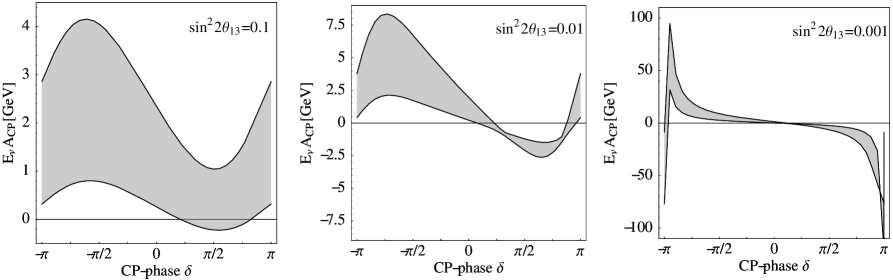
Figure 2: Dependence of the high energy limit of the CP-asymmetry on the CP-phase $\delta$ for bimaximal mixing. On the ordinate is plotted the value of $E_{\nu}A_{\mathrm{CP}}$ in GeV, which should be energy independent in the low $L/E_{\nu}$ approximation. The solar mass splitting was chosen at the upper edge of the LMA-MSW solution ${\Delta m^{2}_{21}}=1\cdot 10^{-4}\,\mathrm{eV}^{2}$ and the atmospheric mass splitting was varied in the Super-Kamiokande allowed 90% confidence interval $3.2\cdot 10^{-3}<{\Delta m^{2}_{31}}<3.6\cdot 10^{-3}\,\mathrm{eV}^{2}$. The calculation was performed for a baseline of 1000 km.

The coefficient, which describes the $1/E_{\nu}$-energy dependence of $A_{\mathrm{CP}}$ for high energies is sensitive to both, matter effects $\hat{A}$ and intrinsic CP-effects from $\delta$. At high energies, the quantity $E_{\nu}A_{\mathrm{CP}}$ is predicted to be constant in the energy spectrum and this characteristical quantity could give direct access to the CP-phase $\delta$. This is demonstrated in fig. 2, which shows the value of $E_{\nu}A_{\mathrm{CP}}$ as function of the CP-phase $\delta$ at different values of $\sin^{2}2\theta_{13}$. Since $E_{\nu}A_{\mathrm{CP}}$ does not vary with the energy, this simple analysis is to a good approximation independent from the energy distribution of the neutrino beam. It is of course questionable if, in a real experiment, in the constant regime of $E_{\nu}A_{\mathrm{CP}}$, there are enough neutrino events to measure. Also this method cannot replace a full and detailed statistical analysis of the complete neutrino energy spectrum.

6.3 Strength of the CP-terms $P_{\sin\delta}$ and $P_{\cos\delta}$

The two subleading terms (36b) and (36c) currently raise considerable interest as they contain information about the CP-phase $\delta$ of the neutrino sector. Today, much effort is spent on the study of CP-violating effects in neutrino oscillation experiments [11]. One can try a simple approach to this problem by using the here obtained analytic results. It would, for example, be interesting to know, how strong the information on $\delta$ inherent to the appearance oscillation probability is. To quantify this, one can look at the relative magnitude of $|P_{\sin\delta}+P_{\cos\delta}|$ compared to the statistical fluctuations $\sqrt{P_{0}+P_{3}}$ in the background signal (provided the errors are Gaussian). To obtain statistical meaningful numbers, the estimation should be performed at the level of event rates expected in a real experiment, e.g. a neutrino factory long baseline experiment. Typically, flux times cross sections of a neutrino factory beam [12] scales like $E_{\nu}^{3}/L^{2}$. A neutrino factory of $20\,\mathrm{GeV}$ muon energy and $10^{20}$ useful muon decays per year produces 54800 $\nu_{\mu}$-events in a 10 kton detector at 1000 km distance (assuming measurements in the appearance channel). As a statistical estimate the following ratio could be chosen:

$$S=\sqrt{54800\left(\frac{E_{\mu}}{20\,\mathrm{GeV}}\right)^{3}\left(\frac{L}{1000~{}\mathrm{km}}\right)^{-2}}\;\frac{|P_{\sin\delta}+P_{\cos\delta}|}{\sqrt{P_{0}+P_{3}}}~{}.$$ (43)

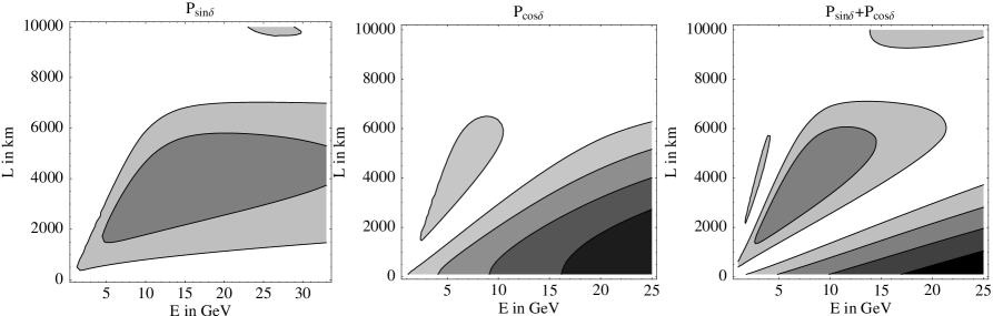
Figure 3: $1\sigma$, $2\sigma$, $3\sigma$ and $4\sigma$ contour lines of the quantity $S$ (eq. (43)) in the $L-E_{\mu}$ parameter plane. Light shading indicates no signal and dark shading indicates strong signal. The left plot studies only the $P_{\sin\delta}$ term. The plot in the middle displays the strength of the $P_{\cos\delta}$ term. The right plot, which combines both terms should give the best approximation to more complex studies. Note that no energy spectrum was used in this crude model. The calculations were performed with $\delta=\pi/2$ (left), $\delta=0$ (middle), $\delta=\pi/4$ (right), bimaximal mixing, and $\sin^{2}2\theta_{13}=0.01$. The mass squared differences are ${\Delta m^{2}_{31}}=3.2\cdot 10^{-3}\,\mathrm{eV}^{2}$ and ${\Delta m^{2}_{21}}=1\cdot 10^{-4}\,\mathrm{eV}^{2}$.

The value of $S$ gives the number of standard deviations (“$\sigma$’s”) at which the CP-signal is distinct from the “background”. Figures 3 show the contour lines $1\sigma$, $2\sigma$, $3\sigma$ and $4\sigma$ of $S$ in the $L-E_{\mu}$ parameter plane. The plots were produced with a running average matter density matched to the baseline $L$. It is interesting to note that in most of the $L-E_{\mu}$ parameter space, there is no obvious decrease of the statistical sensitivity to CP-effects for increasing beam energy $E_{\mu}$ as often quoted in the literature. To study this point in more detail, it is helpful to derive the low $L/E_{\nu}$ (eq. 39) scaling laws for $S$ in the cases $\sin\delta=1$ and $\cos\delta=1$:

$$S_{\sin\delta}\sim\frac{L}{\sqrt{E_{\mu}}}\quad\mathrm{and}\quad S_{\cos\delta}\sim\sqrt{E_{\mu}}~{}.$$ (44)

Indeed, for the $P_{\sin\delta}$-term, the statistical sensitivity should decrease like $1/\sqrt{E_{\mu}}$. However, the validity-region of the low $L/E_{\nu}$ approximation, according to eq. (39), is $E_{\nu}\gtrsim(4,12,20)$ GeV for $L=(1000,3000,5000)$ km. In the left plot of fig. 3 it can be seen that roughly at these energies, $S$ shows a plateau where its maximal value is reached. The argument in favor of small energies thus only holds for very small baselines around 1000 km and smaller. The sensitivity to the $P_{\cos\delta}$-term increases like $\sqrt{E_{\mu}}$. Hence, in the case of large $\cos\delta$, high beam energies are favored to extract information on the CP-phase $\delta$. In conclusion, the difference of the result presented here and statements being found in the literature has two sources. First, usually only the explicitly CP-violating part $P_{\sin\delta}$ of the oscillation probability is assumed to give the CP-signal. Second, the high energy approximation to the oscillation probabilities is often applied without careful consideration of its validity region.

7 Conclusions

The purpose of this work was to find approximate analytic expressions for the neutrino mixing parameters and oscillation probabilities in the presence of matter. It was stated that being interested in approximate solutions it is difficult to describe both the solar and the atmospheric resonance at the same time. Therefore, this work is restricted to energies above the solar resonance according to:

$$|\hat{A}|\gtrsim|\alpha|~{}\Rightarrow~{}E_{\nu}\gtrsim 0.45\,\mathrm{GeV}\left(\frac{{\Delta m^{2}_{21}}}{10^{-4}\,\mathrm{eV}^{2}}\right)\left(\frac{2.8~{}\mathrm{g}/\mathrm{cm}^{3}}{\rho}\right)~{}.$$ (45)

For this regime, the complete parameter mapping (eqs. (27)) was given as series expansion in the small mass hierarchy parameter $\alpha={\Delta m^{2}_{21}}/{\Delta m^{2}_{31}}$. It was shown, that the change of the CP-phase $\delta$ in matter is triple suppressed by the mass hierarchy, the mixing angle $\theta_{13}$ and by $\theta_{23}$ being close to maximal. Furthermore, it was shown that in order ${\Delta m^{2}_{21}}/{\Delta m^{2}_{31}}$, the relevant contribution to the parameter mapping is the correction of $\theta_{12}$ in matter. The derived parameter mapping was used to compute the $P(\nu_{e}\rightarrow\nu_{\mu})$ appearance oscillation probability in matter. Effort was made to find simple solutions, which hold over a wide parameter range and are easy to compare with the results known from vacuum oscillation. An answer, which in the author’s point of view fulfills all these requirements is the following set of terms (eqs. (38)) contributing to $P(\nu_{e}\rightarrow\nu_{\mu})$:

$$P_{0} = \sin^{2}\theta_{23}\frac{\sin^{2}2\theta_{13}}{(\hat{A}-1)^{2}}\sin^{2}((\hat{A}-1)\hat{\Delta})~{},$$

$$P_{\sin\delta} = \alpha\;\frac{\sin\delta\cos\theta_{13}\sin 2\theta_{12}\sin 2\theta_{13}\sin 2\theta_{23}}{\hat{A}(1-\hat{A})}\sin(\hat{\Delta})\sin(\hat{A}\hat{\Delta})\sin((1-\hat{A})\hat{\Delta})~{},$$

$$P_{\cos\delta} = \alpha\;\frac{\cos\delta\cos\theta_{13}\sin 2\theta_{12}\sin 2\theta_{13}\sin 2\theta_{23}}{\hat{A}(1-\hat{A})}\cos(\hat{\Delta})\sin(\hat{A}\hat{\Delta})\sin((1-\hat{A})\hat{\Delta})~{},$$

$$P_{3} = \alpha^{2}\frac{\cos^{2}\theta_{23}\sin^{2}2\theta_{12}}{\hat{A}^{2}}\sin^{2}(\hat{A}\hat{\Delta})$$

with $\hat{\Delta}={\Delta m^{2}_{31}}L/(4E_{\nu})$ and $\hat{A}=A/{\Delta m^{2}_{31}}=2VE_{\nu}/{\Delta m^{2}_{31}}$. This gives qualitatively good results for baselines at which the oscillation over the small (solar) mass squared difference can safely be linearized:

$$\alpha\hat{\Delta}\lesssim 1~{}\Rightarrow~{}L\lesssim 8000~{}\mathrm{km}\left(\frac{E_{\nu}}{\,\mathrm{GeV}}\right)\left(\frac{10^{-4}\,\mathrm{eV}^{2}}{{\Delta m^{2}_{21}}}\right)~{}.$$ (46)

To obtain high precision results for large values of $\theta_{13}$, it is recommended not to neglect subleading $\theta_{13}$ effects. The corresponding terms to $P(\nu_{e}\rightarrow\nu_{\mu})$ are given by eqs. (36a,b,c,f). Results for the anti-neutrino channel are always obtained by flipping the signs of $P_{\sin\delta}$ and $\hat{A}$.

Using the derived approximations to the oscillation probability, it was shown that from relation (40) a stringent limit on the baseline $L$ can be derived, up to which the small $L/E_{\nu}$ approximation in matter is valid. Then, using this approximation, an expression for the CP-asymmetry $A_{\mathrm{CP}}$ in matter was given, which demonstrates that, for high neutrino energies, $A_{\mathrm{CP}}$ is decreasing proportional to $1/E_{\nu}$. It was proposed that measuring this energy-dependence could help to obtain information on the CP-phase $\delta$. Last, it was demonstrated that estimations on the experimental sensitivity to the CP-terms in $P(\nu_{e}\rightarrow\nu_{\mu})$ can be given. The here obtained results do not favor low neutrino energies for the CP-violation search. The reason for the discrepancy between this result and statements, which can presently be found in the literature, were discussed. These topics were discussed only briefly and mainly serve as demonstrations of the applicability of the derived formulas.

Acknowledgments:

I would like to thank E. Akhmedov, S. Bilenky, P. Huber, M. Lindner, and T. Ohlsson for discussions. This work was supported by the “Sonderforschungsbereich 375 für Astro-Teilchenphysik” der Deutschen Forschungsgemeinschaft.

References

[1]
C.W. Kim and W.K. Sze, Phys. Rev. D 35 (1987) 1404;
H.W. Zaglauer and K.H. Schwarzer, Z. Phys. C 40 (1988) 273;
V. Barger, K. Whisnant, S. Pakvasa and R.J.N. Phillips, Phys. Rev: D 22 (1980) 2718;
T. Ohlsson and H. Snellman, J. Math. Phys. 41 (2000) 2768;
Phys. Lett. B 474 (2000) 153; 480 (2000) 419 (E).
[2]
T.K. Kuo and J. Pantaleone, Phys. Rev. Lett. 57 (1986) 1805;
A.S. Joshipura and M. V. N. Murthy, Phys. Rev. D 37 (1988) 1374;
S. Toshev, Phys. Lett. B 185 (1987) 177;
192, 478(E) (1987); S. T. Petcov and S. Toshev, ibid.;
187, 120 (1987); S.T. Petcov, ibid.214 (1988) 259;
J.C. D’Olivo and J. A. Oteo, Phys. Rev. D 54 (1996) 1187;
V.M. Aquino, J. Bellandi, and M. M. Guzzo, Braz. J. Phys. 27 (1997) 384;
G.L. Fogli, E. Lisi, and D. Montanino, Phys. Rev. D
49 (1994) 3626; 54 (1996) 2048;
G.L. Fogli, E. Lisi, D. Montanino, and G. Scioscia, ibid.55 (1997) 4385.
[3]
K. Scholberg, for the Super-Kamiokande Collab.,
e-Print Archive: hep-ex/9905016.
[5] M. Apollonio et al. (CHOOZ collaboration), Phys. Lett. B 466 (1999) 415.
[6]
S.P. Mikheyev and A.Yu. Smirnov,
Yad. Fiz. 42 (1985) 1441; Sov. J. Nucl. Phys. 42 (1985)
913;
S.P. Mikheyev and A.Yu. Smirnov, Nuovo Cimento C 9 (1986) 17;
L. Wolfenstein, Phys. Rev. D17 (1978) 2369;
20 (1979) 2634.
[7]
S. Toshev, Mod. Phys. Lett. A 6 (1991) 455.
[8]
P.F. Harrison and W.G. Scott, Phys.Lett. B 476 (2000) 349.
[9]
A. Cervera et al., Nucl. Phys. B 579 (200) 17; Erratum-ibid. B 593 (2001) 731.
[10] M. Freund, M. Lindner, S.T. Petcov and A. Romanino,
Nucl.Phys. B 578 (2000) 27.
[11]
J. Arafune and J. Sato, Phys. Rev. D 55 (1997) 1653;
K.R. Schubert hep-ph/9902215;
K. Dick, M. Freund, M. Lindner, and A. Romanino, Nucl. Phys. B 562 (1999) 29;
J. Bernabeu, in Proc. 17th Int. Workshop Weak Interact. and Neutrinos (WIN ’99),
eds. C.A. Dominguez and R. D. Viollier (World Scientific, Singapore, 2000) 227;
and many other works.