Nuclear Scattering
at Very High Energies

Abstract

We discuss the current understanding of nuclear scattering at very high energies. We point out several serious inconsistencies in nowadays models, which provide big problems for any interpretation of data at high energy nuclear collisions.

We outline how to develop a fully self-consistent formalism, which in addition uses all the knowledge available from studying electron-positron annihilation and deep inelastic scattering, providing a solid basis for further developments concerning secondary interactions.

1 Introduction

We will report on efforts to construct realistic and reliable models for nuclear collisions at very high energies, say above 100 GeV cms energy per nucleon. There are several reasons why such models are needed, related to large scale experimental programs presently and in the future.

In astrophysics, one of the open problems is the origin of cosmic rays at very high energies. Whereas at low energies direct measurements are possible using balloons or satellites, at high energies – due to the small flux – only indirect measurements are possible, counting the secondary particles created in a so-called extended air-shower. Here, theoretical models for hadron-nucleus and nucleus-nucleus collisions play a decisive role in order to provide some information on the origin of the primary particle.

In nuclear physics, there are ongoing efforts to produce and to investigate the so-called quark-gluon plasma, a new state of matter of quarks and gluons. The SPS program at CERN has revealed many interesting results, but a final conclusion will never be made without a profound theoretical understanding, based on realistic microscopic models.

The outline of this paper is as follows: we will first discuss the present status concerning models for the initial stage of a nucleus-nucleus collision. We find that even the most advanced approaches show severe theoretical inconsistencies, which make any interpretation of experimental data questionable. It is in fact a well known problem which has been brought up a decade ago, but no solution has been proposed so far. We will discuss how to solve the above-mentioned problem, introducing a self-consistent formalism for nuclear scattering at very high energies.

2 Present Status

Many popular models [1, 2, 3] are based on the so-called Gribov-Regge theory (GRT) [4, 5]. This is an effective field theory, which allows multiple interactions to happen “in parallel”, with the phenomenological object called “Pomeron” representing an elementary interaction. Using the general rules of field theory, one may express cross sections in terms of a couple of parameters characterizing the Pomeron. Interference terms are crucial, they assure the unitarity of the theory. Here one observes an inconsistency: the fact that energy needs to be shared between many Pomerons in case of multiple scattering is well taken into account when calculating particle production (in particular in Monte Carlo applications), but energy conservation is not taken care of in cross section calculations. This is a serious problem and makes the whole approach inconsistent.

Provided factorization works for nuclear collisions, one may employ the parton model [6, 7], which allows to calculate inclusive cross sections as a convolution of an elementary cross section with parton distribution functions, with these distribution functions taken from deep inelastic scattering. In order to get exclusive parton level cross sections, some additional assumptions are needed, which follow quite closely the Gribov-Regge approach, encountering the same difficulties.

Before presenting new theoretical ideas, we want to discuss the open problems in the parton model approach and in Gribov-Regge theory somewhat more in detail.

Gribov-Regge Theory

Gribov-Regge theory is by construction a multiple scattering theory. The elementary interactions are realized by complex objects called “Pomerons”, who’s precise nature is not known, and which are therefore simply parameterized: the elastic amplitude $T$ corresponding to a single Pomeron exchange is given as

$$T(s,t)\sim i\,s^{\alpha_{0}+\alpha^{\prime}t}$$

with a couple of parameters to be determined by experiment. Even in hadron-hadron scattering, several of these Pomerons are exchanged in parallel. Using general rules of field theory (cutting rules), one obtains an expression for the inelastic cross section,

$$\sigma^{h_{1}h_{2}}_{\mathrm{inel}}(s)=\int d^{2}b\,\left\{1-\exp\left(-G(s,b)\right)\right\}=\sum\sigma^{h_{1}h_{2}}_{m}(s),$$ (1)

with

$$\sigma^{h_{1}h_{2}}_{m}(s)=\int d^{2}b\,\frac{\left(G(s,b)\right)^{m}}{m!}\exp\left(-G(s,b)\right),$$ (2)

where the so-called eikonal $G(s,b)$ (proportional to the Fourier transform of $T(s,t)$) represents one elementary interaction. The cross sections $\sigma^{h_{1}h_{2}}_{m}(s)$ for $m$ inelastic collisions are referred to as topological cross sections. One can generalize to nucleus-nucleus collisions, where corresponding formulas for cross sections may be derived.

In order to calculate exclusive particle production, one needs to know how to share the energy between the individual elementary interactions in case of multiple scattering. We do not want to discuss the different recipes used to do the energy sharing (in particular in Monte Carlo applications). The point is, whatever procedure is used, this is not taken into account in the calculation of cross sections discussed above. So, actually, one is using two different models for cross section calculations and for treating particle production. Taking energy conservation into account in exactly the same way will modify the cross section results considerably.

This problem has first been discussed in [8],[9]. The authors claim that following from the non-planar structure of the corresponding diagrams, conserving energy and momentum in a consistent way is crucial, and therefore the incident energy has to be shared between the different elementary interactions, both real and virtual ones.

Another very unpleasant and unsatisfactory feature of most “recipes” for particle production is the fact, that the second Pomeron and the subsequent ones are treated differently than the first one, although in the above-mentioned formula for the cross sections all Pomerons are considered to be identical.

The Parton Model

The standard parton model approach to hadron-hadron or also nucleus-nucleus scattering amounts to presenting the partons of projectile and target by momentum distribution functions, $f_{h_{1}}$ and $f_{h_{2}}$, and calculating inclusive cross sections for the production of parton jets with the squared transverse momentum $p_{\perp}^{2}$ larger than some cutoff $Q_{0}^{2}$ as

$$\sigma^{h_{1}h_{2}}_{\mathrm{incl}}=\sum_{ij}\int dp_{\perp}^{2}\int dx^{+}\int dx^{-}f^{i}_{h_{1}}(x^{+},p_{\perp}^{2})f_{h_{2}}^{j}(x^{-},p_{\perp}^{2})\frac{d\hat{\sigma}_{ij}}{dp_{\perp}^{2}}(x^{+}x^{-}s)\theta\!\left(p_{\perp}^{2}-Q^{2}_{0}\right),$$

where $d\hat{\sigma}_{ij}/dp_{\perp}^{2}$ is the elementary parton-parton cross section and $i,j$ represent parton flavors.

This simple factorization formula is the result of cancelations of complicated diagrams (AGK cancelations) and hides therefore the complicated multiple scattering structure of the reaction. The most obvious manifestation of such a structure is the fact that at high energies ($\sqrt{s}\gg 10$ GeV) the inclusive cross section in proton-(anti-)proton scattering exceeds the total one, so the average number $\bar{N}^{pp}_{\mathrm{int}}$ of elementary interactions must be greater than one:

$$\bar{N}_{\mathrm{int}}^{h_{1}h_{2}}=\sigma^{h_{1}h_{2}}_{\mathrm{incl}}/\sigma_{\mathrm{tot}}^{h_{1}h_{2}}>1\>.$$

The usual solution is the so-called eikonalization, which amounts to re-introducing multiple scattering, based on the above formula for the inclusive cross section:

$$\sigma^{h_{1}h_{2}}_{\mathrm{inel}}(s)=\int d^{2}b\,\left\{1-\exp\left(-A(b)\,\sigma^{h_{1}h_{2}}_{\mathrm{incl}}(s)\right)\right\}=\sum\sigma^{h_{1}h_{2}}_{m}(s),$$ (3)

with

$$\sigma^{h_{1}h_{2}}_{m}(s)=\int d^{2}b\,\frac{\left(A(b)\,\sigma^{h_{1}h_{2}}_{\mathrm{incl}}(s)\right)^{m}}{m!}\exp\left(-A(b)\,\sigma^{h_{1}h_{2}}_{\mathrm{incl}}(s)\right)$$ (4)

representing the cross section for $n$ scatterings; $A(b)$ being the proton-proton overlap function (the convolution of two proton profiles). In this way the multiple scattering is “recovered”. This makes the approach formally equivalent to Gribov-Regge theory, encountering therefore the same problems: energy conservation is not at all taken care of in the above formulas for cross section calculations.

3 A Solution: Parton-based Gribov-Regge Theory

In this paper, we present a new approach for hadronic interactions and for the initial stage of nuclear collisions, which is able to solve the above-mentioned problems. We provide a rigorous treatment of the multiple scattering aspect, such that questions as energy conservation are clearly determined by the rules of field theory, both for cross section and particle production calculations. In both (!) cases, energy is properly shared between the different interactions happening in parallel, see fig. 1

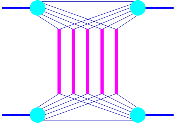
Figure 1: Graphical representation of a contribution to the elastic amplitude of proton-proton scattering. Here, energy conservation is taken into account: the energy of the incoming protons is shared among several “constituents” (shown by splitting the nucleon lines into several constituent lines), and so each Pomeron disposes of only a fraction of the total energy, such that the total energy is conserved.

for proton-proton and fig. 2 for proton-nucleus collisions (generalization to nucleus-nucleus is obvious).

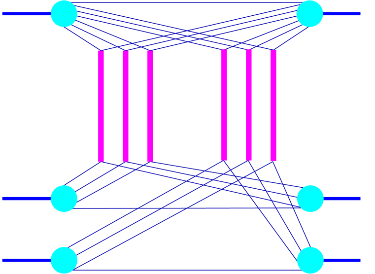
Figure 2: Graphical representation of a contribution to the elastic amplitude of proton-nucleus scattering, or more precisely a proton interacting with (for simplicity) two target nucleons, taking into account energy conservation. Here, the energy of the incoming proton is shared between all the constituents, which now provide the energy for interacting with two target nucleons.

This is the most important and new aspect of our approach, which we consider to be a first necessary step to construct a consistent model for high energy nuclear scattering.

The elementary interactions, shown as the thick lines in the above figures, are in fact a sum of a soft, a hard, and a semi-hard contribution, providing a consistent treatment of soft and hard scattering. To some extend, our approach provides a link between the Gribov-Regge approach and the parton model, we call it “Parton-based Gribov-Regge Theory”.

4 Parton-Parton Scattering

Let us first investigate parton-parton scattering, before constructing a multiple scattering theory for hadronic and nuclear scattering.

We distinguish three types of elementary parton-parton scatterings, referred to as “soft”, “hard” and “semi-hard”, which we are going to discuss briefly in the following. The detailed derivations can be found in [10].

The Soft Contribution

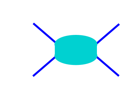
Figure 3: The soft contribution.

Let us first consider the pure non-perturbative contribution, where all virtual partons appearing in the internal structure of the diagram have restricted virtualities $Q^{2}<Q^{2}_{0}$, where $Q_{0}^{2}\simeq 1$ GeV² is a reasonable cutoff for perturbative QCD being applicable. Such soft non-perturbative dynamics is known to dominate hadron-hadron interactions at not too high energies. Lacking methods to calculate this contribution from first principles, it is simply parameterized and graphically represented as a ‘blob’, see fig. 3. It is traditionally assumed to correspond to multi-peripheral production of partons (and final hadrons) [11] and is described by the phenomenological soft Pomeron exchange amplitude $T_{\mathrm{soft}}\!\left(\hat{s},t\right)$ [4]. The corresponding profile function is twice the imaginary part of the Fourier transform $\tilde{T}_{\mathrm{soft}}$ of $T_{\mathrm{soft}}$, divided by the initial parton flux $2\hat{s}$,

$$D_{\mathrm{soft}}(\hat{s},b) = \frac{1}{2\hat{s}}2\mathrm{Im}\frac{1}{4\pi^{2}}\int d^{2}q_{\perp}\,\exp\!\left(-i\vec{q}_{\perp}\vec{b}\right)\,T_{\mathrm{soft}}\!\left(\hat{s},-q^{2}_{\perp}\right)$$ (5)

$$= \frac{2\gamma_{\mathrm{part}}^{2}}{\lambda^{\!(2)}_{\mathrm{soft}}\!(\hat{s}/s_{0})}\left(\frac{\hat{s}}{s_{0}}\right)^{\alpha_{\mathrm{soft}}\!(0)-1}\exp\!\left(-\frac{b^{2}}{4\lambda^{\!(2)}_{\mathrm{soft}}\!(\hat{s}/s_{0})}\right),$$

with

$$\lambda^{\!(n)}_{\mathrm{soft}}\!(z)=nR_{\mathrm{part}}^{2}+\alpha^{\prime}\!_{\mathrm{soft}}\ln\!z,$$

where $\hat{s}$ is the usual Mandelstam variable for parton-parton scattering. The parameters $\alpha_{\mathrm{soft}}\!(0)$, $\alpha^{\prime}\!_{\mathrm{soft}}$ are the intercept and the slope of the Pomeron trajectory, $\gamma_{\mathrm{part}}$ and $R_{\mathrm{part}}^{2}$ are the vertex value and the slope for the Pomeron-parton coupling, and $s_{0}\simeq 1$ GeV² is the characteristic hadronic mass scale. The external legs of the diagram of fig. 3 are “partonic constituents”, which are assumed to be quark-anti-quark pairs.

The Hard Contribution

Let us now consider the other extreme, when all the processes are perturbative, i.e. all internal intermediate partons are characterized by large virtualities $Q^{2}>Q^{2}_{0}$. In that case, the corresponding hard parton-parton scattering amplitude can be calculated using the perturbative QCD techniques [12, 13], and the intermediate states contributing to the absorptive part of the amplitude can be defined in the parton basis. In the leading logarithmic approximation of QCD, summing up terms where each (small) running QCD coupling constant $\alpha_{s}(Q^{2})$ appears together with a large logarithm $\ln(Q^{2}/\lambda^{2}_{\mathrm{QCD}})$ (with $\lambda_{QCD}$ being the infrared QCD scale), and making use of the factorization hypothesis, one obtains the contribution of the corresponding cut diagram for $t=q^{2}=0$ as the cut parton ladder cross section $\sigma_{\mathrm{hard}}^{jk}(\hat{s},Q_{0}^{2})$ , as shown in fig. 4,

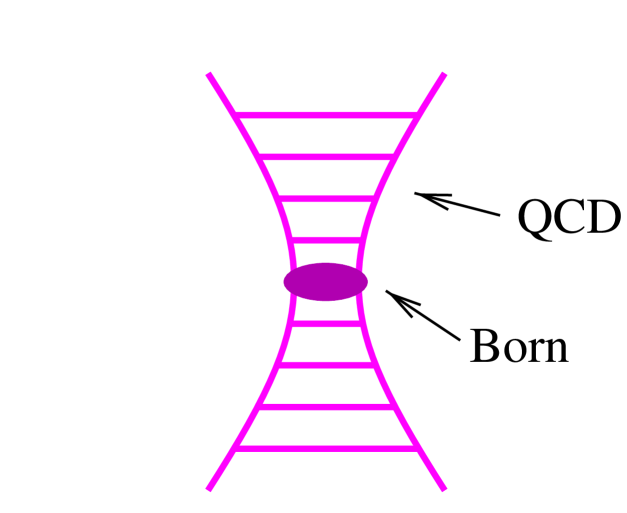
Figure 4: The hard (or val-val) contribution.

where all horizontal rungs are the final (on-shell) partons and the virtualities of the virtual $t$-channel partons increase from the ends of the ladder towards the largest momentum transfer parton-parton process (indicated symbolically by the ‘blob’ in the middle of the ladder):

$$\sigma_{\mathrm{hard}}^{jk}(\hat{s},Q_{0}^{2}) = \frac{1}{2\hat{s}}2\mathrm{Im}\,T^{jk}_{\mathrm{hard}}\!\!\left(\hat{s},t=0,Q_{0}^{2}\right)$$

$$= K\,\sum_{ml}\int dx_{B}^{+}dx_{B}^{-}dp_{\bot}^{2}{d\sigma_{\mathrm{Born}}^{ml}\over dp_{\bot}^{2}}(x_{B}^{+}x_{B}^{-}\hat{s},p_{\bot}^{2})$$

$$\times E_{\mathrm{QCD}}^{jm}(Q_{0}^{2},M_{F}^{2},x_{B}^{+})\,E_{\mathrm{QCD}}^{kl}(Q_{0}^{2},M_{F}^{2},x_{B}^{-})\theta\!\left(M_{F}^{2}-Q^{2}_{0}\right),$$

Here $d\sigma_{\mathrm{Born}}^{ml}/dp_{\bot}^{2}$ is the differential $2\rightarrow 2$ parton scattering cross section, $p_{\bot}^{2}$ is the parton transverse momentum in the hard process, $m,l$ and $x_{B}^{\pm}$ are correspondingly the types and the shares of the light cone momenta of the partons participating in the hard process, and $M_{F}^{2}$ is the factorization scale for the process (we use $M_{F}^{2}=p^{2}_{\perp}/4$). The ‘evolution function’ $E^{jm}_{\mathrm{QCD}}(Q^{2}_{0},M_{F}^{2},z)$ represents the evolution of a parton cascade from the scale $Q_{0}^{2}$ to $M_{F}^{2}$, i.e. it gives the number density of partons of type $m$ with the momentum share $z$ at the virtuality scale $M_{F}^{2}$, resulted from the evolution of the initial parton $j$, taken at the virtuality scale $Q_{0}^{2}$. The evolution function satisfies the usual DGLAP equation [14] with the initial condition $E^{jm}_{\mathrm{QCD}}(Q^{2}_{0},Q_{0}^{2},z)=\delta^{j}_{m}\;\delta(1-z)$. The factor $K\simeq 1.5$ takes effectively into account higher order QCD corrections.

In the following, we shall need to know the contribution of the uncut parton ladder $T_{\mathrm{hard}}^{jk}(\hat{s},t,Q_{0}^{2})$ with some momentum transfer $q$ along the ladder (with $t=q^{2}$). The behavior of the corresponding amplitudes was studied in [15] in the leading logarithmic($1/x$ ) approximation of QCD. The precise form of the corresponding amplitude is not important for our application; we just use some of the results of [15], namely that one can neglect the real part of this amplitude and that it is nearly independent on $t$, i.e. that the slope of the hard interaction $R_{\mathrm{hard}}^{2}$ is negligible small, i.e. compared to the soft Pomeron slope one has $R_{\mathrm{hard}}^{2}\simeq 0$. So we parameterize $T_{\mathrm{hard}}^{jk}(\hat{s},t,Q_{0}^{2})$ in the region of small $t$ as [16]

$$T_{\mathrm{hard}}^{jk}(\hat{s},t,Q_{0}^{2})=i\hat{s}\,\sigma_{\mathrm{hard}}^{jk}(\hat{s},Q_{0}^{2})\>\exp\left(R_{\mathrm{hard}}^{2}\,t\right)$$ (6)

The corresponding profile function is twice the imaginary part of the Fourier transform $\tilde{T}_{\mathrm{hard}}$ of $T_{\mathrm{hard}}$, divided by the initial parton flux $2\hat{s}$,

$$D^{jk}_{\mathrm{hard}}\!\left(\hat{s},b\right)=\frac{1}{2\hat{s}}2\mathrm{Im}\tilde{T}^{jk}_{\mathrm{hard}}(\hat{s},b),$$

which gives

$$D^{jk}_{\mathrm{hard}}\left(\hat{s},b\right)=\frac{1}{8\pi^{2}\hat{s}}\int d^{2}q_{\perp}\,\exp\!\left(-i\vec{q}_{\perp}\vec{b}\right)\,2\mathrm{Im}\,T_{\mathrm{hard}}^{jk}(\hat{s},-q^{2}_{\perp},Q_{0}^{2})$$

$$=\sigma_{\mathrm{hard}}^{jk}\!\left(\hat{s},Q_{0}^{2}\right)\frac{1}{4\pi R_{\mathrm{hard}}^{2}}\exp\!\left(-\frac{b^{2}}{4R_{\mathrm{hard}}^{2}}\right),$$ (7)

In fact, the above considerations are only correct for valence quarks, as discussed in detail in the next section. Therefore, we also talk about “valence-valence” contribution and we use $D_{\mathrm{val}-\mathrm{val}}$ instead of $D_{\mathrm{hard}}$:

$$D^{jk}_{\mathrm{val}-\mathrm{val}}\left(\hat{s},b\right)\equiv D^{jk}_{\mathrm{hard}}\left(\hat{s},b\right),$$

so these are two names for one and the same object.

The Semi-hard Contribution

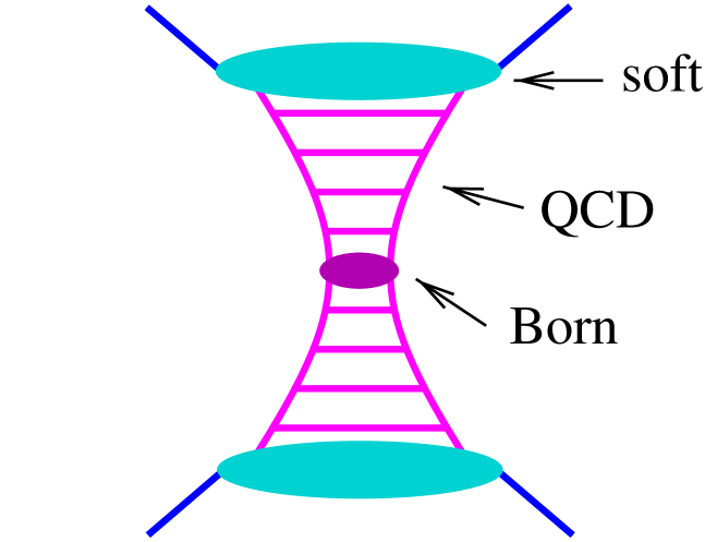
Figure 5: The semi-hard “sea-sea” contribution: parton ladder plus “soft ends”.

The discussion of the preceding section is not valid in case of sea quarks and gluons, since here the momentum share $x_{1}$ of the “first” parton is typically very small, leading to an object with a large mass of the order $Q^{2}_{0}/x_{1}$ between the parton and the proton [17]. Microscopically, such ’slow’ partons with $x_{1}\ll 1$ appear as a result of a long non-perturbative parton cascade, where each individual parton branching is characterized by a small momentum transfer squared $Q^{2}<Q^{2}_{0}$ [4, 18]. When calculating proton structure functions or high-$p_{t}$ jet production cross sections this non-perturbative contribution is usually included in parameterized initial parton momentum distributions at $Q^{2}=Q^{2}_{0}$. However, the description of inelastic hadronic interactions requires to treat it explicitly in order to account for secondary particles produced during such non-perturbative parton pre-evolution, and to describe correctly energy-momentum sharing between multiple elementary scatterings. As the underlying dynamics appears to be identical to the one of soft parton-parton scattering considered above, we treat this soft pre-evolution as the usual soft Pomeron emission, as discussed in detail in [10].

So for sea quarks and gluons, we consider so-called semi-hard interactions between parton constituents of initial hadrons, represented by a parton ladder with “soft ends”, see fig. 5. As in the case of soft scattering, the external legs are quark-anti-quark pairs, connected to soft Pomerons. The outer partons of the ladder are on both sides sea quarks or gluons (therefore the index “sea-sea”). The central part is exactly the hard scattering considered in the preceding section. As discussed in length in [10], the mathematical expression for the corresponding amplitude is given as

$$iT_{\mathrm{sea}-\mathrm{sea}}(\hat{s},t) = \sum_{jk}\int^{1}_{0}\!\frac{dz^{+}}{z^{+}}\frac{dz^{-}}{z^{-}}\,\mathrm{Im}\,T_{\mathrm{soft}}^{j}\!\!\left(\frac{s_{0}}{z^{+}},t\right)\,\mathrm{Im}\,T_{\mathrm{soft}}^{k}\!\!\left(\frac{s_{0}}{z^{-}},t\right)\,iT_{\mathrm{hard}}^{jk}(z^{+}z^{-}\hat{s},t,Q_{0}^{2}),$$

with $z^{\pm}$ being the momentum fraction of the external leg-partons of the parton ladder relative to the momenta of the initial (constituent) partons. The indices $j$ and $k$ refer to the flavor of these external ladder partons. The amplitudes $T_{\mathrm{soft}}^{j}$ are the soft Pomeron amplitudes discussed earlier, but with modified couplings, since the Pomerons are now connected to a parton ladder on one side. The arguments $s_{0}/z^{\pm}$ are the squared masses of the two soft Pomerons, $z^{+}z^{-}\hat{s}$ is the squared mass of the hard piece.

Performing as usual the Fourier transform to the impact parameter representation and dividing by $2\hat{s}$, we obtain the profile function

$$D_{\mathrm{sea}-\mathrm{sea}}\left(\hat{s},b\right)=\frac{1}{2\hat{s}}\,2\mathrm{Im}\,\tilde{T}_{\mathrm{sea}-\mathrm{sea}}\!\left(\hat{s},b\right),$$

which may be written as

$$D_{\mathrm{sea}-\mathrm{sea}}\left(\hat{s},b\right) = \sum_{jk}\int^{1}_{0}dz^{+}dz^{-}E_{\mathrm{soft}}^{j}\left(z^{+}\right)\,E_{\mathrm{soft}}^{k}\left(z^{-}\right)\,\sigma_{\mathrm{hard}}^{jk}(z^{+}z^{-}\hat{s},Q_{0}^{2})$$ (8)

$$\qquad\times\;\frac{1}{4\pi\,\lambda^{\!(2)}_{\mathrm{soft}}(1/(z^{+}z^{-}))}\exp\!\left(-\frac{b^{2}}{4\lambda^{\!(2)}_{\mathrm{soft}}\!\left(1/(z^{+}z^{-})\right)}\right)$$

with the soft Pomeron slope $\lambda^{\!(2)}_{\mathrm{soft}}$ and the cross section $\sigma_{\mathrm{hard}}^{jk}$ being defined earlier. The functions $E_{\mathrm{soft}}^{j}\left(z^{\pm}\right)$ representing the “soft ends” are defined as

$$\mathrm{E}^{j}_{\mathrm{soft}}(z^{\pm})=\mathrm{Im}\,T_{\mathrm{soft}}^{j}\!\!\left(\frac{s_{0}}{z^{\pm}},t=0\right).$$

We neglected the small hard scattering slope $R_{\mathrm{hard}}^{2}$ compared to the Pomeron slope $\lambda^{(2)}_{\mathrm{soft}}$. We call $E_{\mathrm{soft}}$ also the “ soft evolution”, to indicate that we consider this as simply a continuation of the QCD evolution, however, in a region where perturbative techniques do not apply any more. As discussed in [10], $E_{\mathrm{soft}}^{j}\left(z\right)$ has the meaning of the momentum distribution of parton $j$ in the soft Pomeron.

Consistency requires to also consider the mixed semi-hard contributions with a valence quark on one side and a non-valence participant (quark-anti-quark pair) on the other one, see fig. 6.

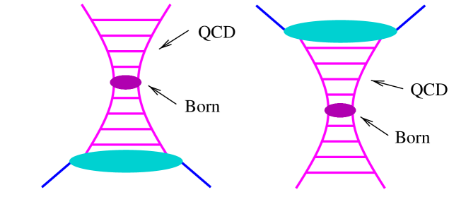
Figure 6: Two “mixed” contributions.

We have

$$iT^{j}_{\mathrm{val}-\mathrm{sea}}(\hat{s})=\int^{1}_{0}\!\frac{dz^{-}}{z^{-}}\sum_{k}\mathrm{Im}\,T_{\mathrm{soft}}^{k}\!\!\left(\frac{s_{0}}{z^{-}},q^{2}\right)iT_{\mathrm{hard}}^{jk}\left(z^{-}\hat{s},q^{2},Q_{0}^{2}\right)\qquad$$

and

$$D^{j}_{\mathrm{val}-\mathrm{sea}}\left(\hat{s},b\right) = \sum_{k}\int^{1}_{0}\!dz^{-}\,E_{\mathrm{soft}}^{k}\left(z^{-}\right)\,\sigma_{\mathrm{hard}}^{jk}\!\left(z^{-}\hat{s},Q_{0}^{2}\right)$$

$$\qquad\times\;\frac{1}{4\pi\,\lambda^{\!(1)}_{\mathrm{soft}}(1/z^{-})}\exp\!\left(-\frac{b^{2}}{4\lambda^{\!(1)}_{\mathrm{soft}}\!\left(1/z^{-}\right)}\right)$$

where $j$ is the flavor of the valence quark at the upper end of the ladder and $k$ is the type of the parton on the lower ladder end. Again, we neglected the hard scattering slope $R^{2}_{\mathrm{hard}}$ compared to the soft Pomeron slope. A contribution $D^{j}_{\mathrm{sea}-\mathrm{val}}\left(\hat{s},b\right)$, corresponding to a valence quark participant from the target hadron, is given by the same expression,

$$D^{j}_{\mathrm{sea}-\mathrm{val}}\left(\hat{s},b\right)=D^{j}_{\mathrm{val}-\mathrm{sea}}\left(\hat{s},b\right),$$

since eq. (4) stays unchanged under replacement $z^{-}\rightarrow z^{+}$ and only depends on the total c.m. energy squared $\hat{s}$ for the parton-parton system.

5 Hadron-Hadron Scattering

To treat hadron-hadron scattering we use parton momentum Fock state expansion of hadron eigenstates [8]

$$|h\rangle=\sum^{\infty}_{k=1}\frac{1}{k!}\int^{1}_{0}\!\prod^{k}_{l=1}\!dx_{l}\,f^{h}_{k}\!\left(x_{1},\ldots x_{k}\right)\,\delta\!\left(1-\sum^{k}_{j=1}\!x_{j}\right)\,a^{+}\!(x_{1})\cdots a^{+}\!(x_{k})\left|0\right\rangle,$$

where $f_{k}\!\left(x_{1},\ldots x_{k}\right)$ is the probability amplitude for the hadron $h$ to consist of $k$ constituent partons with the light cone momentum fractions $x_{1},\ldots,x_{k}$ and $a^{+}\!\left(x\right)$ is the creation operator for a parton with the fraction $x$. A general scattering process is described as a superposition of a number of pair-like scatterings between parton constituents of the projectile and target hadrons. Then hadron-hadron scattering amplitude is obtained as a convolution of individual parton-parton scattering amplitudes considered in the previous section and “inclusive” momentum distributions $\frac{1}{n!}\tilde{F}_{h}^{(n)}\!\left(x_{1},\ldots x_{n}\right)$ of $n$ “participating” parton constituents involved in the scattering process($n\geq 1$), with

$$\frac{1}{n!}\tilde{F}_{h}^{(n)}\!\left(x_{1},\ldots x_{n}\right)=\sum^{\infty}_{k=n}\frac{1}{k!}\frac{k!}{n!\,(k-n)!}\int^{1}_{0}\!\prod^{k}_{l=n+1}\!\!dx_{l}\;\left|f_{k}\!\left(x_{1},\ldots x_{k}\right)\right|^{2}\,\delta\!\left(1-\sum^{k}_{j=1}\!x_{j}\right)$$

We assume that $\tilde{F}_{h_{1}(h_{2})}^{(n)}\!\left(x_{1},\ldots x_{n}\right)$ can be represented in a factorized form as a product of the contributions $F^{h}_{\mathrm{part}}(x_{l})$, depending on the momentum shares $x_{l}$ of the “participating” or “active” parton constituents, and on the function $F^{h}_{\mathrm{remn}}\!\left(1-\sum^{n}_{j=1}x_{j}\right)$,

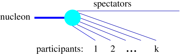
Figure 7: Nucleon Fock state.

representing the contribution of all “spectator” partons, sharing the remaining share $1-\sum_{j}x_{j}$ of the initial light cone momentum (see fig. 7):

$$\tilde{F}_{h}^{(n)}\!\left(x_{1},\ldots x_{n}\right)=\prod^{n}_{l=1}\!F^{h}_{\mathrm{part}}(x_{l})\,\;F^{h}_{\mathrm{remn}}\!\left(1-\sum^{n}_{j=1}x_{j}\right)$$ (10)

The participating parton constituents are assumed to be quark-anti-quark pairs (not necessarily of identical flavors), such that the baryon numbers of the projectile and of the target are conserved. Then, as discussed in detail in [10], the hadron-hadron amplitude may be written as

$$iT_{h_{1}h_{2}}(s,t)=8\pi^{2}s\sum^{\infty}_{n=1}\frac{1}{n!}\,\int^{1}_{0}\!\prod^{n}_{l=1}\!dx_{l}^{+}dx_{l}^{-}\;\prod^{n}_{l=1}\!\left[\frac{1}{8\pi^{2}\hat{s}_{l}}\int\!d^{2}q_{l_{\perp}}\,iT^{h_{1}h_{2}}_{1\mathrm{I}\!\mathrm{P}}\!\left(x_{l}^{+},x_{l}^{-},s,-q_{l_{\perp}}^{2}\right)\right]$$

$$F^{h_{1}}_{\mathrm{remn}}\!\!\left(1-\sum^{n}_{j=1}\!x_{j}^{+}\right)\,F^{h_{2}}_{\mathrm{remn}}\!\!\left(1-\sum^{n}_{j=1}\!x_{j}^{-}\right)\>\delta^{(2)}\!\left(\sum^{n}_{k=1}\!\vec{q}_{k_{\perp}}-\vec{q}_{\perp}\right),$$ (11)

where the partonic amplitudes are defined as

$$T_{1\mathrm{I}\!\mathrm{P}}^{h_{1}h_{2}}=T^{h_{1}h_{2}}_{\mathrm{soft}}+T^{h_{1}h_{2}}_{\mathrm{sea}-\mathrm{sea}}+T^{h_{1}h_{2}}_{\mathrm{val}-\mathrm{val}}+T^{h_{1}h_{2}}_{\mathrm{val}-\mathrm{sea}}+T^{h_{1}h_{2}}_{\mathrm{sea}-\mathrm{val}},$$

with the individual contributions representing the “elementary partonic interactions plus external legs”. The soft or semi-hard sea-sea contributions are given as

$$T^{h_{1}h_{2}}_{\mathrm{soft}/\mathrm{sea}-\mathrm{sea}}\!\left(x^{+},x^{-},s,-q_{\bot}^{2}\right)=T_{\mathrm{soft}/\mathrm{sea}-\mathrm{sea}}\!\left(s,-q_{\bot}^{2}\right)\,F^{h_{1}}_{\mathrm{part}}(x^{+})\,F^{h_{2}}_{\mathrm{part}}(x^{-})$$

$$\times\;\exp\!\left(-\left[R_{h_{1}}^{2}+R_{h_{2}}^{2}\right]q_{\bot}^{2}\right),$$ (12)

the hard contribution is

$$T^{h_{1}h_{2}}_{\mathrm{val}-\mathrm{val}}\!\left(x^{+},x^{-},s,q^{2}\right) = \int^{x^{+}}_{0}\!dx_{v}^{+}\frac{x^{+}}{x_{v_{l}}^{+}}\int^{x^{-}}_{0}\!dx_{v}^{-}\frac{x^{-}}{x_{v}^{-}}\sum_{j,k}T_{\mathrm{hard}}^{jk}\left(x_{v}^{+}x_{v}^{-}s,q^{2},Q_{0}^{2}\right)$$

$$\qquad\times\;\bar{F}^{h_{1},j}_{\mathrm{part}}(x_{v}^{+},x^{+}-x^{+}_{v})\,\bar{F}^{h_{2},k}_{\mathrm{part}}(x_{v}^{-},x^{-}-x_{v}^{-})\,\exp\!\left(-\left[R_{h_{1}}^{2}+R_{h_{2}}^{2}\right]q_{l_{\perp}}^{2}\right),$$

the mixed semi-hard “val-sea” contribution is given as

$$T^{h_{1}h_{2}}_{\mathrm{val}-\mathrm{sea}}\!\left(x^{+},x^{-},s,q^{2}\right) = \int^{x^{+}}_{0}\!dx^{+}_{v}\frac{x^{+}}{x_{v}^{+}}\sum_{j}T_{\mathrm{val}-\mathrm{sea}}^{j}\left(x_{v}^{+}x^{-}s,q^{2},Q_{0}^{2}\right)$$

$$\qquad\times\;\bar{F}^{h_{1},j}_{\mathrm{part}}(x_{v}^{+},x^{+}-x^{+}_{v})\,F^{h_{2}}_{\mathrm{part}}(x^{-})\,\exp\!\left(-\left[R_{h_{1}}^{2}+R_{h_{2}}^{2}\right]q_{l_{\perp}}^{2}\right),$$

and the contribution “sea-val” is finally obtained from “val-sea” by exchanging variables,

$$T^{h_{1}h_{2}}_{\mathrm{sea}-\mathrm{val}}\!\left(x^{+},x^{-},s,q^{2}\right)=T^{h_{2}h_{1}}_{\mathrm{val}-\mathrm{sea}}\!\left(x^{-},x^{+},s,q^{2}\right).$$

Here, we allow formally any number of valence type interactions (based on the fact that multiple valence type processes give negligible contribution). In the valence contributions, we have convolutions of hard parton scattering amplitudes $T_{\mathrm{hard}}^{jk}$ and valence quark distributions $\bar{F}^{j}_{\mathrm{part}}$ over the valence quark momentum share $x_{v}^{\pm}$ rather than a simple product, since only the valence quarks are involved in the interactions, with the anti-quarks staying idle (the external legs carrying momenta $x^{+}$ and $x^{-}$ are always quark-anti-quark pairs).

The profile function $\gamma$ is as usual defined as

$$\gamma_{h_{1}h_{2}}(s,b)=\frac{1}{2s}2\mathrm{Im}\tilde{\mathrm{T}}_{h_{1}h_{2}}(s,b),$$

which may be evaluated using the AGK cutting rules with the result (assuming imaginary amplitudes)

$$\gamma_{h_{1}h_{2}}(s,b) = \sum^{\infty}_{m=1}\frac{1}{m!}\,\int^{1}_{0}\!\prod^{m}_{\mu=1}\!dx_{\mu}^{+}dx_{\mu}^{-}\prod^{m}_{\mu=1}G^{h_{1}h_{2}}_{1\mathrm{I}\!\mathrm{P}}(x_{\mu}^{+},x_{\mu}^{-},s,b)$$ (13)

$$\sum^{\infty}_{l=0}\frac{1}{l!}\,\int^{1}_{0}\!\prod^{l}_{\lambda=1}\!d\tilde{x}_{\lambda}^{+}d\tilde{x}_{\lambda}^{-}\prod^{l}_{\lambda=1}-G^{h_{1}h_{2}}_{1\mathrm{I}\!\mathrm{P}}(\tilde{x}_{\lambda}^{+},\tilde{x}_{\lambda}^{-},s,b)$$

$$F_{\mathrm{remn}}\left(x^{\mathrm{proj}}-\sum_{\lambda}\tilde{x}_{\lambda}^{+}\right)\,F_{\mathrm{remn}}\left(x^{\mathrm{targ}}-\sum_{\lambda}\tilde{x}_{\lambda}^{-}\right),$$

with $x^{\mathrm{proj}/\mathrm{targ}}=1-\sum x^{\pm}_{\mu}$ being the momentum fraction of the projectile/target remnant, and with a partonic profile function $G$ given as

$$G^{h_{1}h_{2}}_{1\mathrm{I}\!\mathrm{P}}(x_{\lambda}^{+},x_{\lambda}^{-},s,b) = \frac{1}{2s}2\mathrm{Im}\,\tilde{T}^{h_{1}h_{2}}_{1\mathrm{I}\!\mathrm{P}}(x_{\lambda}^{+},x_{\lambda}^{-},s,b),$$ (14)

see fig. 8.

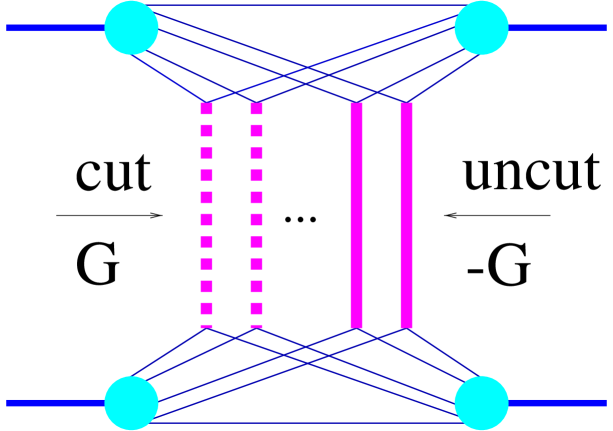
Figure 8: The hadronic profile function $\gamma$ expressed in terms of partonic profile functions $G\equiv G^{h_{1}h_{2}}_{1\mathrm{I}\!\mathrm{P}}$.

This is a very important result, allowing to express the total profile function $\gamma_{h_{1}h_{2}}$ via the elementary profile functions $G^{hg_{1}h_{2}}_{1\mathrm{I}\!\mathrm{P}}$.

6 Nucleus-Nucleus Scattering

We generalize the discussion of the last section in order to treat nucleus-nucleus scattering. In the Glauber-Gribov approach [19, 5], the nucleus-nucleus scattering amplitude is defined by the sum of contributions of diagrams, corresponding to multiple scattering processes between parton constituents of projectile and target nucleons. Nuclear form factors are supposed to be defined by the nuclear ground state wave functions. Assuming the nucleons to be uncorrelated, one can make the Fourier transform to obtain the amplitude in the impact parameter representation. Then, for given impact parameter $\vec{b}_{0}$ between the nuclei, the only formal difference from the hadron-hadron case will be the averaging over nuclear ground states, which amounts to an integration over transverse nucleon coordinates $\vec{b}^{A}_{i}$ and $\vec{b}^{B}_{j}$ in the projectile and in the target respectively. We write this integration symbolically as

$$\int dT_{AB}:=\int\prod_{i=1}^{A}d^{2}b^{A}_{i}\,T_{A}(b^{A}_{i})\prod_{j=1}^{B}d^{2}b^{B}_{j}\,T_{B}(b^{B}_{j}),$$ (15)

with $A,B$ being the nuclear mass numbers and with the so-called nuclear thickness function $T_{A}(b)$ being defined as the integral over the nuclear density $\rho_{A(B)}$:

$$T_{A}(b):=\int dz\,\rho_{A}(b_{x},b_{y},z).$$ (16)

It is convenient to use the transverse distance $b_{k}$ between the two nucleons from the $k$-th nucleon-nucleon pair, i.e.

$$b_{k}=\left|\vec{b}_{0}+\vec{b}^{A}_{\pi(k)}-\vec{b}^{B}_{\tau(k)}\right|,$$

where the functions $\pi(k)$ and $\tau(k)$ refer to the projectile and the target nucleons participating in the $k^{\mathrm{th}}$ interaction (pair $k$). In order to simplify the notation, we define a vector $b$ whose components are the overall impact parameter $b_{0}$ as well as the transverse distances $b_{1},...,b_{AB}$ of the nucleon pairs,

$$b=\{b_{0},b_{1},...,b_{AB}\}.$$

Then the nucleus-nucleus interaction cross section can be obtained applying the cutting procedure to elastic scattering diagram and written in the form

$$\sigma^{AB}_{\mathrm{inel}}(s)=\int d^{2}b_{0}\int dT_{AB}\,\gamma_{AB}(s,b),$$ (17)

where the so-called nuclear profile function $\gamma_{AB}$ represents an interaction for given transverse coordinates of the nucleons.

The calculation of the profile function $\gamma_{AB}$ as the sum over all cut diagrams of the type shown in fig. 9 does not differ from the hadron-hadron case and follows the rules formulated

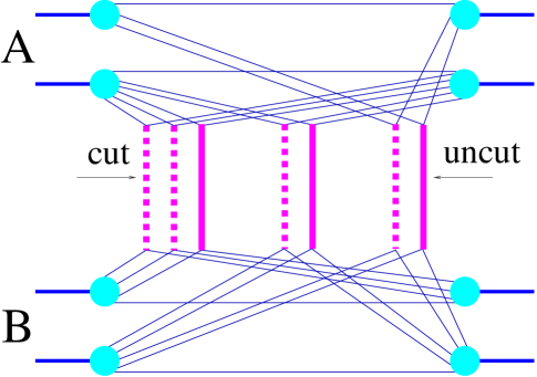
Figure 9: Example for a cut multiple scattering diagram, with cut (dashed lines) and uncut (full lines) elementary diagrams. This diagram can be translated directly into a formula for the inelastic cross section (see text).

in the preceding section:

• For a remnant carrying the light cone momentum fraction $x$ ($x^{+}$ in case of projectile, or $x^{-}$ in case of target), one has a factor $F_{\mathrm{remn}}(x)$.

• For each cut elementary diagram (real elementary interaction = dashed vertical line) attached to two participants with light cone momentum fractions $x^{+}$ and $x^{-}$, one has a factor $G(x^{+},x^{-},s,b)$. Apart from $x^{+}$ and $x^{-}$, $G$ is also a function of the total squared energy $s$ and of the relative transverse distance $b$ between the two corresponding nucleons (we use $G$ as an abbreviation for $G_{1\mathrm{I}\!\mathrm{P}}^{NN}$ for nucleon-nucleon scattering).

• For each uncut elementary diagram (virtual emissions = full vertical line) attached to two participants with light cone momentum fractions $x^{+}$ and $x^{-}$, one has a factor $-G(x^{+},x^{-},s,b),$ with the same $G$ as used for the cut diagrams.

• Finally one sums over all possible numbers of cut and uncut Pomerons and integrates over the light cone momentum fractions.

So we find

$$\gamma_{AB}(s,b) = \sum_{m_{1}l_{1}}\ldots\sum_{m_{AB}l_{AB}}(1-\delta_{0\Sigma m_{k}})\,\int\,\prod_{k=1}^{AB}\left\{\prod^{m_{k}}_{\mu=1}dx_{k,\mu}^{+}dx_{k,\mu}^{-}\,\prod^{l_{k}}_{\lambda=1}d\tilde{x}_{k,\lambda}^{+}d\tilde{x}_{k,\lambda}^{-}\right\}$$ (18)

$$\times \prod_{k=1}^{AB}\left\{\frac{1}{m_{k}!}\frac{1}{l_{k}!}\prod_{\mu=1}^{m_{k}}G(x_{k,\mu}^{+},x_{k,\mu}^{-},s,b_{k})\prod_{\lambda=1}^{l_{k}}-G(\tilde{x}_{k,\lambda}^{+},\tilde{x}_{k,\lambda}^{-},s,b_{k})\right\}$$

$$\times \prod_{i=1}^{A}F_{\mathrm{remn}}\left(x^{+}_{i}-\sum_{\pi(k)=i}\tilde{x}_{k,\lambda}^{+}\right)\prod_{j=1}^{B}F_{\mathrm{remn}}\left(x^{-}_{j}-\sum_{\tau(k)=j}\tilde{x}_{k,\lambda}^{-}\right)$$

with

$$x^{\mathrm{proj}}_{i} = 1-\sum_{\pi(k)=i}x_{k,\mu\,,}^{+}$$

$$x^{\mathrm{targ}}_{j} = 1-\sum_{\tau(k)=j}x_{k,\mu}^{-}\,.$$

The summation indices $m_{k}$ refer to the number of cut elementary diagrams and $l_{k}$ to number of uncut elementary diagrams, related to nucleon pair $k$. For each possible pair $k$ (we have altogether $AB$ pairs), we allow any number of cut and uncut diagrams. The integration variables $x^{\pm}_{k,\mu}$ refer to the $\mu^{\mathrm{th}}$ elementary interaction of the $k^{\mathrm{th}}$ pair for the cut elementary diagrams, the variables $\tilde{x}^{\pm}_{k,\lambda}$ refer to the corresponding uncut elementary diagrams. The arguments of the remnant functions $F_{\mathrm{remn}}$ are the remnant light cone momentum fractions, i.e. unity minus the momentum fractions of all the corresponding elementary contributions (cut and uncut ones). We also introduce the variables $x^{\mathrm{proj}}_{i}$and $x_{j}^{\mathrm{targ}}$, defined as unity minus the momentum fractions of all the corresponding cut contributions, in order to integrate over the uncut ones (see below).

The expression for $\gamma_{AB}$ sums up all possible numbers of cut Pomerons $m_{k}$ with one exception due to the factor $(1-\delta_{0\Sigma m_{k}})$: one does not consider the case of all $m_{k}$’s being zero, which corresponds to “no interaction” and therefore does not contribute to the inelastic cross section. We may therefore define a quantity $\bar{\gamma}_{AB}$, representing “no interaction”, by taking the expression for $\gamma_{AB}$ with $(1-\delta_{0\Sigma m_{k}})$ replaced by $(\delta_{0\Sigma m_{k}})$:

$$\bar{\gamma}_{AB}(s,b) = \sum_{l_{1}}\ldots\sum_{l_{AB}}\,\int\,\prod_{k=1}^{AB}\left\{\prod^{l_{k}}_{\lambda=1}d\tilde{x}_{k,\lambda}^{+}d\tilde{x}_{k,\lambda}^{-}\right\}\;\prod_{k=1}^{AB}\left\{\frac{1}{l_{k}!}\,\prod_{\lambda=1}^{l_{k}}-G(\tilde{x}_{k,\lambda}^{+},\tilde{x}_{k,\lambda}^{-},s,b_{k})\right\}$$ (19)

$$\times \prod_{i=1}^{A}F^{+}\!\left(1-\sum_{\pi(k)=i}\tilde{x}_{k,\lambda}^{+}\right)\prod_{j=1}^{B}F^{-}\left(1-\sum_{\tau(k)=j}\tilde{x}_{k,\lambda}^{-}\right).$$

One now may consider the sum of “interaction” and “no interaction”, and one obtains easily

$$\gamma_{AB}(s,b)+\bar{\gamma}_{AB}(s,b)=1.$$ (20)

Based on this important result, we consider $\gamma_{AB}$ to be the probability to have an interaction and correspondingly $\bar{\gamma}_{AB}$ to be the probability of no interaction, for fixed energy, impact parameter and nuclear configuration, specified by the transverse distances $b_{k}$ between nucleons, and we refer to eq. (20) as “unitarity relation”. But we want to go even further and use an expansion of $\gamma_{AB}$ in order to obtain probability distributions for individual processes, which then serves as a basis for the calculations of exclusive quantities.

The expansion of $\gamma_{AB}$ in terms of cut and uncut Pomerons as given above represents a sum of a large number of positive and negative terms, including all kinds of interferences, which excludes any probabilistic interpretation. We have therefore to perform summations of interference contributions – sum over any number of virtual elementary scatterings (uncut Pomerons) – for given non-interfering classes of diagrams with given numbers of real scatterings (cut Pomerons)[20]. Let us write the formulas explicitly. We have

$$\gamma_{AB}(s,b) = \sum_{m_{1}}\ldots\sum_{m_{AB}}(1-\delta_{0\sum m_{k}})\,\int\,\prod_{k=1}^{AB}\left\{\prod^{m_{k}}_{\mu=1}dx_{k,\mu}^{+}dx_{k,\mu}^{-}\right\}$$ (21)

$$\times \prod_{k=1}^{AB}\left\{\frac{1}{m_{k}!}\,\prod_{\mu=1}^{m_{k}}G(x_{k,\mu}^{+},x_{k,\mu}^{-},s,b_{k})\right\}\;\Phi_{AB}\left(x^{\mathrm{proj}},x^{\mathrm{targ}},s,b\right),$$

where the function $\Phi$ representing the sum over virtual emissions (uncut Pomerons) is given by the following expression

$$\Phi_{AB}\left(x^{\mathrm{proj}},x^{\mathrm{targ}},s,b\right) = \sum_{l_{1}}\ldots\sum_{l_{AB}}\,\int\,\prod_{k=1}^{AB}\left\{\prod^{l_{k}}_{\lambda=1}d\tilde{x}_{k,\lambda}^{+}d\tilde{x}_{k,\lambda}^{-}\right\}\;\prod_{k=1}^{AB}\left\{\frac{1}{l_{k}!}\,\prod_{\lambda=1}^{l_{k}}-G(\tilde{x}_{k,\lambda}^{+},\tilde{x}_{k,\lambda}^{-},s,b_{k})\right\}$$ (22)

$$\times \prod_{i=1}^{A}F_{\mathrm{remn}}\left(x_{i}^{\mathrm{proj}}-\sum_{\pi(k)=i}\tilde{x}_{k,\lambda}^{+}\right)\prod_{j=1}^{B}F_{\mathrm{remn}}\left(x^{\mathrm{targ}}_{j}-\sum_{\tau(k)=j}\tilde{x}_{k,\lambda}^{-}\right).$$

This summation has to be carried out, before we may use the expansion of $\gamma_{AB}$ to obtain probability distributions. This is far from trivial, the necessary methods are described in [10]. To make the notation more compact, we define matrices $X^{+}$ and $X^{-}$, as well as a vector $m$, via

$$X^{+} = \left\{x_{k,\mu}^{+}\right\},$$

$$X^{-} = \left\{x_{k,\mu}^{-}\right\},$$

$$m = \{m_{k}\},$$

which leads to

$$\gamma_{AB}(s,b) = \sum_{m}(1-\delta_{0m})\int dX^{+}dX^{-}\Omega_{AB}^{(s,b)}(m,X^{+},X^{-}),$$

$$\bar{\gamma}_{AB}(s,b) = \Omega_{AB}^{(s,b)}(0,0,0),$$

with

$$\Omega_{AB}^{(s,b)}(m,X^{+},X^{-})=\prod_{k=1}^{AB}\left\{\frac{1}{m_{k}!}\,\prod_{\mu=1}^{m_{k}}G(x_{k,\mu}^{+},x_{k,\mu}^{-},s,b_{k})\right\}\;\Phi_{AB}\left(x^{\mathrm{proj}},x^{\mathrm{targ}},s,b\right).$$

This allows to rewrite the unitarity relation eq. (20) in the following form,

$$\sum_{m}\int dX^{+}dX^{-}\Omega_{AB}^{(s,b)}(m,X^{+},X^{-})=1.$$

This equation is of fundamental importance, because it allows us to interpret $\Omega^{(s,b)}(m,X^{+},X^{-})$ as probability density of having an interaction configuration characterized by $m$, with the light cone momentum fractions of the Pomerons being given by $X^{+}$ and $X^{-}$.

7 Virtual Emissions and Markov Chain Techniques

What did we achieve so far? We have formulated a well defined model, introduced by using the language of field theory, solving in this way the severe consistency problems of the most popular current approaches. To proceed further, one needs to solve two fundamental problems:

• the sum $\Phi_{AB}$ over virtual emissions has to be performed,

• tools have to be developed to deal with the multidimensional probability distribution $\Omega_{AB}^{(s,b)}$,

both being very difficult tasks. Introducing new numerical techniques, we were able to solve both problems, as discussed in very detail in [10].

Calculating the sum over virtual emissions ($\Phi_{AB}$) is done by parameterizing the functions $G$ as analytical functions and performing analytical calculations. By studying the properties of $\Phi_{AB}$, we find that at very high energies the theory is no longer unitary without taking into account screening corrections due to triple Pomeron interactions. In this sense, we consider our work as a first step to construct a consistent model for high energy nuclear scattering, but there is still work to be done.

Concerning the multidimensional probability distribution $\Omega_{AB}^{(s,b)}(m,X^{+},X^{-})$, we employ methods well known in statistical physics (Markov chain techniques). So finally, we are able to calculate the probability distribution $\Omega_{AB}^{(s,b)}(m,X^{+},X^{-})$, and are able to generate (in a Monte Carlo fashion) configurations $(m,X^{+},X^{-})$ according to this probability distribution.

8 Summary

What are finally the principal features of our basic results, summarized in eqs. (17, 21, 22)? Contrary to the traditional treatment (Gribov-Regge approach or parton model), all individual elementary contributions $G$ depend explicitly on the light-cone momenta of the elementary interactions, with the total energy-momentum being precisely conserved. Another very important feature is the explicit dependence of the screening contribution $\Phi_{AB}$ (the contribution of virtual emissions) on the remnant momenta. The direct consequence of properly taking into account energy-momentum conservation in the multiple scattering process is the validity of the so-called AGK-cancelations in hadron-hadron and nucleus-nucleus collisions in the entire kinematical region.

The formulas (17, 21, 22) allow to develop a consistent scheme to simulate high energy nucleus-nucleus interactions. The corresponding Monte Carlo procedure is exactly based on the cross section formulas so that the entire model is fully self-consistent.

References

• [1] A. B. Kaidalov and K. A. Ter-Martirosyan, Nucl. Phys. B75, 471 (1974).
• [2] K. Werner, Phys. Rep. 232, 87 (1993).
• [3] A. Capella, U. Sukhatme, C.-I. Tan, and J. Tran Thanh Van, Phys. Rept. 236, 225 (1994).
• [4] V. N. Gribov, Sov. Phys. JETP 26, 414 (1968).
• [5] V. N. Gribov, Sov. Phys. JETP 29, 483 (1969).
• [6] T. Sjostrand and M. van Zijl, Phys. Rev. D36, 2019 (1987).
• [7] X.-N. Wang, Phys. Rept. 280, 287 (1997), hep-ph/9605214.
• [8] V. A. Abramovskii and G. G. Leptoukh, Sov.J.Nucl.Phys. 55, 903 (1992).
• [9] M. Braun, Yad. Fiz. (Rus) 52, 257 (1990).
• [10] H. J. Drescher, M. Hladik, S. Ostapchenko, T. Pierog, and K. Werner, (2000), hep-ph/0007198, to be published in Physics Reports.
• [11] D. Amati, A. Stanghellini, and S. Fubini, Nuovo Cim. 26, 896 (1962).
• [12] G. Altarelli, Phys. Rep. 81, 1 (1982).
• [13] E. Reya, Phys. Rep. 69, 195 (1981).
• [14] G. Altarelli and G. Parisi, Nucl. Phys. B126, 298 (1977).
• [15] L. N. Lipatov, Sov. Phys. JETP 63, 904 (1986).
• [16] M. G. Ryskin and Y. M. Shabelski, Yad. Fiz. (Rus.) 55, 2149 (1992).
• [17] A. Donnachie and P. Landshoff, Phys. Lett. B 332, 433 (1994).
• [18] M. Baker and K. A. Ter-Martirosyan, Phys. Rep. 28, 1 (1976).
• [19] R. J. Glauber, in Lectures on theoretical physics (N.Y.: Inter-science Publishers, 1959).
• [20] V. A. Abramovskii, V. N. Gribov, and O. V. Kancheli, Sov.J.Nucl.Phys. 18, 308 (1974).