Constraining Models of New Physics
in Light of Recent Experimental Results on ${a_{\psi K_{S}}}$

Abstract

We study extensions of the Standard Model where the charged current weak interactions are governed by the CKM matrix and where all tree-level decays are dominated by their Standard Model contribution. We constrain both analytically and numerically the ratio and the phase difference between the New Physics and the Standard Model contributions to the mixing amplitude of the neutral $B$ system using the experimental results on $R_{u}$, $\Delta m_{d,s}$, $\varepsilon_{K}$ and ${a_{\psi K_{S}}}$. We present new results concerning models with minimal flavor violation and update the relevant parameter space. We also study the left-right symmetric model with spontaneously broken CP, probing the viability of this model in view of the recent results for ${a_{\psi K_{S}}}$ and other observables.

I Introduction

For more than 30 years the only unambiguous indication for CP violation (CPV) was found in the neutral kaon system. Even though the CP violating parameter

$$\varepsilon_{K}=(2.280\pm 0.013)\times 10^{-3}e^{i\phi_{\varepsilon}}~{}~{}~{}\mbox{with}~{}~{}~{}\phi_{\varepsilon}\simeq\pi/4$$ (1)

has been measured rather accurately [1], hadronic uncertainties obscure the determination of the fundamental CKM parameters [2]. However, there is growing evidence that CPV also occurs in the $B$ meson system. Specifically, indications for a CP asymmetry in $B_{d}\to J/\psi\,K_{S}$ decays have been reported by the ALEPH [3], BaBar [4], BELLE [5], CDF [6] and OPAL [7] collaborations. Combining all the measurement gives:

$$a_{\psi K_{S}}=0.51\pm 0.18\,.$$ (2)

It is essential to understand the impact of the present and upcoming experimental data on the SM and its extensions. In this paper we focus on a large class of NP models where the charged current weak interactions are governed by a $3\times 3$ unitary matrix, just like in the CKM picture. Moreover, we make the reasonable assumption that all tree-level decays are dominated by their SM contribution. However, flavor changing neutral current processes are sensitive to New Physics (NP) because, in the SM, they appear only at the loop level.

After a brief update on the SM picture, we study in detail, both analytically and numerically, the allowed parameter space of the ratio and the phase difference between the NP and the SM contributions to the mixing amplitude of the neutral $B$ system. We use the experimental results on $R_{u}$, $\Delta m_{d,s}$, $\varepsilon_{K}$ and ${a_{\psi K_{S}}}$ for the generic NP models. Besides the two general assumptions mentioned above we introduce additional constraints that apply to specific NP models. First, we assume that the ratio between the mass differences of the $B_{d}$ and the $B_{s}$ neural meson system is unaffected by NP, which is valid, e.g., in models with Minimal Flavor Violation (MFV). Second, we impose a small CP violating phase, as for example in left-right symmetric (LRS) models with spontaneous CPV.

We devote special attention to models of MFV. We show that the three parameters $\rho$, $\eta$ and $F_{tt}$ can be obtained analytically from the experimental results on $R_{u}$, $\Delta m_{d}$ and $\varepsilon_{K}$. Additional constraints on the parameter space arise from the measurement of ${a_{\psi K_{S}}}$ and the upper bound on $\Delta m_{d}/\Delta m_{s}$.

Finally, we investigate the impact of the uncertainty of various parameters in LRS models with spontaneous CPV on recent claims that these models would be ruled out by a significant CP asymmetry in $B_{d}\to J/\psi\,K_{S}$ decays.

II Standard Model picture

CPV appears naturally in the Standard Model with three generations of quarks. It can be attributed to a single phase, $\delta_{KM}$, appearing in the CKM matrix that describes the weak charged-current interactions. Among the four Wolfenstein parameters $(\lambda,A,\rho,\eta)$ that provide a convenient description of the CKM matrix [8] only two have been determined with a good accuracy [1], namely

$$\lambda=0.2237\pm 0.0033~{}~{}~{}~{}~{}\mbox{and}~{}~{}~{}~{}~{}A=0.819\pm 0.040\,.$$ (3)

The other two parameters $(\rho,\eta)$ describing the apex of the unitarity triangle, that follows from the unitarity relation $V_{ud}V_{ub}^{*}+V_{cd}V_{cb}^{*}+V_{td}V_{tb}^{*}=0\,,$ have a rather large uncertainty. As a consequence the CP violating phase $\delta_{KM}=\arctan(\eta/\rho)$ of the SM is relatively weakly constrained.

In the following we review briefly how the allowed region for the two Wolfenstein parameters $\rho$ and $\eta$ is obtained (for more details see e.g. [9, 10] and references therein). At present these parameters are experimentally constrained by the measurement of $|V_{ub}/V_{cb}|$, the observed $B_{d}^{0}-\bar{B}_{d}^{0}$ mixing parameter $\Delta m_{d}$, the lower bound on the $B_{s}^{0}-\bar{B}_{s}^{0}$ mixing parameter $\Delta m_{s}$, the measurement of $\varepsilon_{K}$ and the combined result for $a_{\psi K_{S}}$. Note that for the purpose of this paper it is sufficient to work to leading order in $\lambda^{2}$ and we therefore neglect all subdominant contributions.

The distance from the origin to the apex $(\rho,\eta)$ of the rescaled unitarity triangle,

$$\sqrt{\rho^{2}+\eta^{2}}\simeq R_{u}\equiv\left|{V_{ub}^{*}V_{ud}\over V_{cb}^{*}V_{cd}}\right|\,,$$ (4)

is proportional to $|V_{ub}/V_{cb}|$, which dominates its uncertainty. The ratio $|V_{ub}/V_{cb}|$ can be determined from various tree-level $B$ decays (see e.g. [11] and Tab 1. ), restricting $R_{u}$ to the interval

$$R_{u}\in[0.34,~{}0.43]\,.$$ (5)

The distance between the apex of the rescaled unitarity triangle and the point $(1,0)$ in the $\rho-\eta$ plane is given by:

$$\sqrt{(\rho-1)^{2}+\eta^{2}}\simeq R_{t}\equiv\left|{V_{tb}^{*}V_{td}\over V_{cb}^{*}V_{cd}}\right|\,.$$ (6)

$R_{t}$ can be determined from the experimental results for mass differences $\Delta m_{q}$ in the $B_{q}^{0}-\bar{B}_{q}^{0}$ ($q=d,s$) systems by means of the SM predictions (see e.g. [9, 10]):

$$\Delta m_{q}={G_{F}^{2}\over 6\pi^{2}}\eta_{B}m_{B_{q}}m_{W}^{2}f^{2}_{B_{q}}B_{B_{q}}S_{0}(x_{t})\cdot|V_{tq}V_{tb}^{*}|^{2}\,.$$ (7)

Here $G_{F}$ is the Fermi constant, $\eta_{B}$ is a QCD correction factor, $m_{B_{q}}$ is the $B_{q}^{0}$ mass, $m_{W}$ is the $W$-boson mass, $f_{B_{q}}$ is the $B_{q}$ decay constant, $B_{B_{q}}$ parameterizes the value of the relevant hadronic matrix element and $S_{0}(x_{t})$ gives the electroweak loop contribution as a function of the top quark mass $m_{t}^{2}=x_{t}m_{W}^{2}$. Also the ratio $\Delta m_{d}/\Delta m_{s}$ is very useful since it is simply related to $R_{t}$ via

$${\Delta m_{d}\over\Delta m_{s}}\simeq R_{t}^{2}\,{\lambda^{2}\over\xi^{2}}\cdot{m_{B_{d}}\over m_{B_{s}}}\,,$$ (8)

where $\xi\equiv f_{B_{s}}/f_{B_{d}}\cdot\sqrt{B_{B_{s}}/B_{B_{d}}}\,.$

The measurement of the $\varepsilon_{K}$ parameter in combination with the SM prediction determines a region between two hyperbolae in the $\rho-\eta$ plane, described by (see e.g. [9, 10]):

$$\eta\left[(1-\rho)\eta_{2}S_{0}(x_{t})A^{2}+P_{c}\right]A^{2}B_{K}\simeq 0.226\,.$$ (9)

Here $\eta_{2}$ is a QCD correction factor and $P_{c}$ characterizes the contributions with one or two intermediate charm-quarks.

Finally the recent results for the CP asymmetry in the $B^{0}_{d}\to J/\psi\,K_{S}$ decay in eq. (2) imply a further constraint in the $\rho-\eta$ plane via the SM prediction

$$a_{\psi K_{S}}=\sin 2\beta\,,$$ (10)

where

$$\beta\equiv\arg\left(-{V_{cd}V_{cb}^{*}\over V_{td}V_{tb}^{*}}\right)\,.$$ (11)

In terms of the Wolfenstein parameters we have

$$\sin 2\beta\simeq{2\eta(1-\rho)\over{\eta^{2}+(1-\rho)^{2}}}\,.$$ (12)

Combining the above formulae and using the input parameters in Tab. 1 we obtain the allowed region for $(\rho,\eta)$ shown in Fig. 1. Note that we naively combine the aforementioned constraints in order to determine the allowed region. (For more sophisticated analyses see e.g. refs. [12, 13, 11, 14].)

III Generic New Physics Models With Unitary Mixing Matrix

We focus our analysis on a large class of new physics (NP) models with the following two features (c.f. refs [15, 16, 17] and references therein):

• The $3\times 3$ mixing matrix for the charged current weak interactions is unitary.

• Tree-level decays are dominated by the SM contributions.

Note that assumption (i) holds in all SM extensions with three quark generations. Assumption (ii) implies in particular that the phase of the $B\to\psi K_{S}$ decay amplitude is given by the Standard Model CKM phase, $\arg(V_{cb}V_{cs}^{*})$. Both assumptions are satisfied by a wide class of models, like supersymmetry with $R$-parity, various LRS models, models with minimal flavor violation (MFV) and several multi-Higgs models. Since some of the models mentioned above have additional features we investigate the following three scenarios:

• Only assumptions (i) and (ii) are valid.

• Assumptions (i) and (ii) apply and $\Delta m_{d}/\Delta m_{s}$ is unaffected by the presence of NP.

• Assumptions (i) and (ii) apply and $\delta_{KM}$ is small.

Scenario (b) contains, for example, certain multi-Higgs models with “flavor conservation” and models with MFV [10, 18, 19, 20]. Scenario (c) applies to models of approximate CP symmetry and LRS models with spontaneous CPV [21, 22, 23, 24, 25, 26, 27, 28]. To be specific we take $|\tan(\delta_{KM})|<\tan(\delta^{max})=0.25$ for these scenarios.

The NP effects relevant to our analysis modify the $B_{d}-\bar{B}_{d}$ mixing amplitude, $M_{12}-{i\over 2}\Gamma_{12}$. Assumption (ii) implies that the impact of NP on the absorptive part of this amplitude is negligible:

$$\Gamma_{12}\approx\Gamma_{12}^{\rm SM}\,.$$ (13)

The modification of $M_{12}$ can be parameterized as follows (see refs. [15, 16, 29] and refs. therein):

$${M_{12}\over M_{12}^{\rm SM}}=r_{d}^{2}\,e^{2i\theta_{d}}\,.$$ (14)

The variables $r_{d}$ and $\theta_{d}$ relate directly to the experimental observables. The results for $\Delta m_{d,s}$ constrain $r_{d}^{2}$, while the recent measurement of $a_{\psi K_{S}}$ restricts the value of the phase $2\theta_{d}$. However, to investigate a specific model it is convenient to use different variables, $h$ and $\sigma$, and describe the NP modifications to the amplitude $M_{12}={M_{12}^{\rm SM}+M_{12}^{\rm NP}}$ via [15, 16, 29]:

$${M_{12}^{\rm NP}\over M_{12}^{\rm SM}}=h\,e^{i\sigma}\,.$$ (15)

The variables $h$ and $\sigma$ are related to $r_{d}$ and $\theta_{d}$ through:

$$r_{d}^{2}\,e^{2i\theta_{d}}=1+h\,e^{i\sigma}\,.$$ (16)

Our goal is to determine the allowed parameter space for $h$ and $\sigma$. To this end we first constrain $r_{d}^{2}$ and $2\theta_{d}$ using the relevant experimental results on $R_{u}$, $\Delta m_{d,s}$, $\varepsilon_{K}$ and ${a_{\psi K_{S}}}$. Then we show how to translate the ranges for $r_{d}^{2}$ and $2\theta_{d}$ into the allowed region in the $h-\sigma$ plane. All the relevant parameters we use in our analysis are summarized in Tab. 1. For most of these parameters we adopt the values of ref. [11]. For simplicity we scan over the ranges indicated in Tab. 1 both for the theoretical and experimental parameters.

A Constraining $r_{d}$ and $\theta_{d}$

The parameter $r_{d}^{2}$ is constrained by the results for $\Delta m_{d,s}$ [15, 16]. In models that satisfy the assumptions (i) and (ii) the expressions for $\Delta m_{d,s}$ in eq. (7) have to be modified as follows [15]:

$$\Delta m_{q}={G_{F}^{2}\over 6\pi^{2}}\eta_{B}m_{B_{q}}m_{W}^{2}f^{2}_{B_{q}}B_{B_{q}}S_{0}(x_{t})\,|V_{tq}V_{tb}^{*}|^{2}\cdot r_{q}^{2}\,,$$ (17)

where $q=d,s$ and $r_{s}$ is the analog to $r_{d}$ for the $B_{s}$ system. Moreover $\Delta m_{B_{d}}/\Delta m_{B_{s}}$ satisfies:

$${\Delta m_{B_{d}}\over\Delta m_{B_{s}}}\simeq\lambda^{2}R_{t}^{2}\cdot\xi^{-2}{m_{B_{d}}\over m_{B_{s}}}\left({r_{d}\over r_{s}}\right)^{2}\,,$$ (18)

which reduces to the SM expression in eq. (8) when $r_{d}=r_{s}$. Note, that the constraint on $R_{u}$ given in eq. (4) is unchanged by NP, since it is dominated by tree-level amplitudes.

Using the values in Tab. 1, from eq. (17) it follows that:

$$0.69< r_{d}\cdot R_{t}(\rho,\eta)<1.03\,,$$ (19)

while eq. (18) implies that

$${r_{d}\over r_{s}}R_{t}(\rho,\eta)\leq 0.99\,.$$ (20)

The allowed range for the phase $\theta_{d}$ is restricted by the measurement of $a_{\psi K_{S}}$ [15]. Due to the two-fold ambiguity of the $\sin$ function, the one-sigma result for $a_{\psi K_{S}}$ in eq. (2) corresponds to two allowed intervals for $2(\theta_{d}+\beta)$ [15, 16]:

$$19^{\circ}\ \hbox to0.0pt{\raise 3.0pt\hbox{$<$}\hss}{\lower 3.0pt\hbox{$\sim$}}\ 2(\theta_{d}+\beta)\ \hbox to0.0pt{\raise 3.0pt\hbox{$<$}\hss}{\lower 3.0pt\hbox{$\sim$}}\ 44^{\circ}\ \ \ \mbox{or}\ \ \ 19^{\circ}\ \hbox to0.0pt{\raise 3.0pt\hbox{$<$}\hss}{\lower 3.0pt\hbox{$\sim$}}\ 180^{\circ}-2(\theta_{d}+\beta)\ \hbox to0.0pt{\raise 3.0pt\hbox{$<$}\hss}{\lower 3.0pt\hbox{$\sim$}}\ 44^{\circ}\,.$$ (21)

We use the above results for two types of analysis: In our numerical analysis we scan over the $\rho-\eta$ plane and calculate the allowed intervals for $r_{d}$ according to eq. (19) [and eq. (20) in scenario (b)] and $\theta_{d}$ from eq. (21) for all points ($\rho,\eta$) that fulfill the constraints relevant to a particular scenario (c.f. Fig. 2 for scenario (a), Fig. 4 for scenario (b) and Fig. 6 for scenario (c), respectively).

To get better insight into the numerical results we have performed an analytical calculation, where we use the maximal allowed region for $r_{d}$ and $\theta_{d}$ that follow from the global constraints on $R_{t}$ and $\beta$. Such an approach is particularly useful, because the analytical constraints can easily be updated using the forthcoming experimental data. Moreover the system of constraints may be extended for different classes of NP models. For scenario (a) we get (see appendix A 1 for details):

$$r_{d}\in[0.5,~{}1.8]~{}~{}~{}~{}~{}\mbox{and}~{}~{}~{}~{}~{}2\theta_{d}\in[-32^{\circ},~{}212^{\circ}]\,.$$ (22)

Note that the interval for $2\theta_{d}$ in eq. (22) is independent of the upper bound on ${a_{\psi K_{S}}}$ as long as $(2\theta_{d})_{max_{1}}>(2\theta_{d})^{min_{2}}$. With the upper bound on $R_{u}$ in eq. (4) two distinct intervals for $2\theta_{d}$ only appear if $({a_{\psi K_{S}}})_{max}<0.63$. This explains why the global constraint on $2\theta_{d}$ we obtain from the measurement of ${a_{\psi K_{S}}}$ in eq. (2) almost coincides with the one in ref. [15], even though our upper bound on ${a_{\psi K_{S}}}$ is much more stringent.

For scenario (b) the lower bound on $r_{d}$ is somewhat stronger, since from eq. (20) it follows that $R_{t}(\rho,\eta)\leq 0.99$, which gives $r_{d}>0.7$. In scenario (c) we have

$$r_{d}\in[0.5,~{}0.8]~{}~{}~{}~{}~{}\mbox{with}~{}~{}~{}~{}~{}2\theta_{d}\in[12^{\circ},~{}51^{\circ}]\cup[129^{\circ},~{}168^{\circ}]\,,$$ (23)

for the allowed regions with $\rho<0$ and

$$r_{d}\in[1.0,~{}1.8]~{}~{}~{}~{}~{}\mbox{with}~{}~{}~{}~{}~{}2\theta_{d}\in[-1^{\circ},~{}64^{\circ}]\cup[116^{\circ},~{}181^{\circ}]\,,$$ (24)

for the allowed regions with $\rho>0$ (c.f. Fig. 6).

B Constraining $h$ and $\sigma$

Our first observation is that from the maximal value for $r_{d}$ one obtains an upper bound on $h$. Eq. (16) implies that

$$h(r_{d},\theta_{d})=\sqrt{r_{d}^{4}-2r^{2}_{d}\cos 2\theta_{d}+1}\leq(r_{d}^{max})^{2}+1\approx 4.24\,,$$ (25)

where the upper bound arises from setting $\cos 2\theta_{d}=-1$ and $r_{d}=r_{d}^{max}$. Still, one can obtain much better bounds using the correlation between $h$ and $\sigma$. Here we only sketch how to translate the constraints one obtains for $r_{d}^{2}$ and $2\theta_{d}$ into those for $h$ and $\sigma$. The details can be found in appendix A 2. The basic idea is simple. We solve eq. (16) for $h$, once eliminating $\theta_{d}$,

$$h^{\pm}(\sigma,r_{d})\equiv-\cos\sigma\pm\sqrt{\cos^{2}\sigma+r_{d}^{4}-1}\,,$$ (26)

and once eliminating $r_{d}$,

$$h^{\pm}(\sigma,\theta_{d})={\sin 2\theta_{d}\,\sin(2\theta_{d}\pm\sigma)\over\sin^{2}\sigma-\sin^{2}2\theta_{d}}\,.$$ (27)

Using the above equations the ranges for $r_{d}$ and $\theta_{d}$ can be translated into a region in the $h-\sigma$ plane. The overlap of the two areas from eq. (26) and eq. (27) corresponds to the allowed region in the $h-\sigma$ parameter space. While this method is straightforward one has to treat carefully the discrete ambiguities of the trigonometric functions (see appendix).

Using eq. (26) and eq. (27) the global constraints on $r_{d}$ and $\theta_{d}$ in eqs. (22)–(24) can be readily translated into the allowed region for $h$ and $\sigma$. Combining all the resulting intervals one obtains the light areas, whose boundaries are given by $h^{\pm}(\sigma,r_{d})$ and $h^{\pm}(\sigma,\theta_{d})$ with $r_{d}$ and $\theta_{d}$ at the edges of their allowed intervals (see appendix A 2 for more details).

In order to obtain the exact allowed region in the $h-\sigma$ plane we have performed a numerical analysis proceeding as follows: Rather than using the global constraints on $r_{d}$ and $\theta_{d}$ corresponding to the entire allowed region in the $\rho-\eta$ plane, we compute the possible ranges for $r_{d}$ and $\theta_{d}$ for each permissible value of $\rho$ and $\eta$. That is we scan over the $\rho-\eta$ plane and for all points ($\rho,\eta$) that fulfill the constraints relevant to a particular scenario, we calculate the allowed intervals for $r_{d}$ according to eq. (19) [and eq. (20) in scenario (b)] and $\theta_{d}$ from eq. (21). The resulting intervals are then translated into the corresponding region in the $h-\sigma$ plane, just as we did in the “global” analysis, but for each point ($\rho,\eta$) separately. Combining all the resulting intervals one obtains the allowed regions indicated as the dark areas in Fig. 3, Fig. 5 and Fig. 7. They are contained within the light areas resulting from the analytic boundaries from the global constraints. Even though in general the numerical results are not much more constraining than the global ones, there exist some regions where the numerical constraints are significantly stronger than the analytical boundaries. For example, there appear “holes” in the dark gray regions of Fig. 3 and Fig. 5 that correspond to the excluded region within the $R_{u}$ annulus, which has been ignored in “global” analysis (light gray regions). Even more important, the lower bound on $h$ in scenario (c) (see Fig. 7) from the numerical analysis turns out to be significantly stronger than in the global analysis, which is marginally consistent with $h=0$.

C Summary of Results

• Generic models: All models that satisfy the assumptions (i) and (ii) must respect the condition in eq. (4), which corresponds to an annulus around the origin in the $\rho-\eta$ plane as shown in Fig. 2. The resulting allowed region in the $h-\sigma$ plane is presented in Fig. 3. The admissible range for $h$ is given by:

  $$h\in[0,~{}4.2]\,.$$ (28)

• Models where $\Delta m^{SM}_{d}/\Delta m^{SM}_{s}\approx\Delta m_{d}/\Delta m_{s}$: The relevant region in the $\rho-\eta$ plane is shown in Fig. 4 and the resulting allowed region in the $h-\sigma$ plane is presented in Fig. 5. The admissible range for $h$ is the same as in eq. (28), but the excluded area in the $h-\sigma$ plane is somewhat larger.

• Models in which $\delta^{KM}$ is significantly smaller than unity: The relevant region in the $\rho-\eta$ plane for this class of models is shown in Fig. 6 and the resulting allowed region in the $h-\sigma$ plane is presented in Fig. 7. The excluded region is significantly smaller than in scenario (a) and (b). The admissible range for $h$ and $\sigma$ are given by:

  $$h\in[0.14,~{}4.18]~{}~{}~{}~{}~{}\mbox{and}~{}~{}~{}~{}~{}\sigma\in[0^{\circ},~{}180^{\circ}]\,.$$ (29)

  Unlike for scenarios (a) and (b) in this case $h$ has also a non-trivial lower bound and $\sigma$ has an upper bound. Consequently NP contributions to the $B-\bar{B}$ mixing amplitude are required in this scenario.

IV Specific New Physics Models

In this section we focus on two specific New Physics models that belong to the general class of models discussed above. We discuss first models with minimal flavor violation (MFV) and subsequently we present some new results relevant to LRS models with spontaneous CPV.

A Minimal Flavor Violation

Models with MFV comprise the SM and those extensions of the SM in which all flavor changing interactions are described by the CKM matrix. These models do not introduce any new operators implying the absence of any new CP violating phases beyond the KM phase. The only impact of MFV models are modifications of the Wilson coefficients of the SM operators due to additional contributions from diagrams involving new internal particles [10, 18, 19, 20].

1 Constraints from $R_{u}$, $\Delta m_{d,s}$ and $\varepsilon_{K}$

In the framework of this analysis the only relevant modifications of the SM predictions concern the mass difference $\Delta m_{d}$ of the $B_{d}$ system and the parameter $\varepsilon_{K}$ describing CP violation in $K^{0}-\bar{K}^{0}$ mixing. It turns out that for both parameters the new physics charm and charm-top contributions are negligible and that additional contributions to the SM box diagram with top quark exchanges can be described by one single parameter $F_{tt}$.

This parameter effectively replaces the relevant Inami-Lim function $S_{0}(x_{t})$ appearing in eqs. (7) and (9), which have to be substituted by [18]

$$\Delta m_{d}={G_{F}^{2}\over 6\pi^{2}}\eta_{B}m_{B_{d}}m_{W}^{2}f^{2}_{B_{d}}B_{B_{d}}F_{tt}\cdot|V_{td}V_{tb}^{*}|^{2}\,.$$ (30)

and

$$\eta\left[(1-\rho)\eta_{2}F_{tt}A^{2}+P_{c}\right]A^{2}B_{K}\simeq 0.226\,,$$ (31)

respectively. The constraint on the unitarity triangle from $R_{u}$ [c.f. eq. (4)] remains unaffected in MFV models, because it is dominated by tree-level contributions. Furthermore, due to the absence of any new phases in the $B-\bar{B}$ mixing amplitude the SM prediction for ${a_{\psi K_{S}}}$ [c.f. eqs. (10)-(12)] is unchanged. Finally, $\Delta m_{d}/\Delta m_{s}$ in eq. (8) remains unaffected since the NP contributions cancel each other in the ratio.

The important point we want to make is that for any given set of the parameters $R_{u},A,B_{K},P_{c}$ and

$$\Delta_{f}\equiv{\Delta m_{d}\over B_{B_{d}}f_{B}^{2}\lambda^{6}}\,$$ (32)

one can obtain exact expressions for $\rho$, $\eta$ and $F_{tt}$. Combining eqs. (4), (30) and (31) results into a quartic equation that can be solved analytically. For example, for $\rho$ one obtains

$$(R_{u}^{2}-\rho^{2})\,\left[(1-\rho)C_{\Delta}+C_{c}(1-2\rho+R_{u}^{2})\right]^{2}=\left[C_{\varepsilon}(1-2\rho+R_{u}^{2})\right]^{2}\,,$$ (33)

where

$$C_{\Delta}\equiv{6\pi^{2}\Delta_{f}\over G_{F}^{2}\eta_{B}m_{B_{d}}M_{W}^{2}A^{2}}\,,\ \ \ \ \ C_{\varepsilon}\equiv{0.226\over A^{4}B_{K}\eta_{2}}\,,~{}~{}~{}~{}~{}\mbox{and}~{}~{}~{}~{}~{}C_{c}\equiv{P_{c}\over A^{2}\eta_{2}}\,.$$ (34)

We have used the analytic expressions to obtain the allowed regions for $\rho$, $\eta$ and $F_{tt}$ by scanning over the intervals for $R_{u},A,B_{K},P_{c}$ and $\Delta_{f}$ in Tab. 2. A priori up to four solutions are possible, but for the present ranges of the parameters $R_{u},A,B_{K},P_{c}$ and $\Delta_{f}$ only two solutions are real (see Fig. 8 and Fig. 9). Adding the constraint from $\Delta m_{d}/\Delta m_{s}$ in eq. (8) practically the entire solution shown in Fig. 8 is ruled out and only the second solution in Fig. 9 remains viable. We find that $F_{tt}$ is restricted to the interval

$$F_{tt}\in[1.2,~{}5.7]\,,$$ (35)

which includes the SM value $F_{tt}^{SM}\equiv S_{0}(x_{t})\simeq 2.46\,(m_{t}/170~{}{\rm GeV})^{1.52}$ [10].

The value of $\sin 2\beta$ within models of MFV has obtained considerable attention recently [30, 10, 12]. In particular it was shown in ref. [30] that there exists a lower bound on $\sin 2\beta$ in these models. The existence of this bound is a non-trivial result of the correlation between $\Delta m_{d}$ and $\varepsilon_{K}$ which holds in models of MFV [30]. Using the analytic solutions for $\rho$, $\eta$ and $F_{tt}$ we have investigated the behavior of $\sin 2\beta$ as a function of $R_{u},A,B_{K},P_{c}$ and $\Delta_{f}$. We find that it takes its minimal value, $(\sin 2\beta)_{min}$, when $R_{u}$ is minimal and all the other parameters are maximal. While the size of the exact expressions we obtained for $\rho$, $\eta$, $F_{tt}$ and $\sin 2\beta$ preclude its presentation here, one can use the results to expand these parameters around a particular value. For example a linear expansion of $\sin 2\beta$ around $R_{u}^{min},A^{max},B_{K}^{max},P_{c}^{max}$ and $\Delta_{f}^{max}$ gives:

$$\sin 2\beta \simeq 0.52+0.23\,(R_{u}-0.34)-1.09\,(A-0.86)-0.47\,(B_{K}-1.00)$$ (36)

$$-0.31\,(P_{c}-0.36)-3.43\times 10^{-6}\,\left({\Delta_{f}\over{\rm ps}^{-1}\,{\rm GeV}^{-2}}-1.04\times 10^{5}\right)\,.$$ (37)

This expansion provides a good approximation to the exact expression for $\sin 2\beta$ within most of the allowed parameter space for $R_{u},A,B_{K},P_{c}$ and $\Delta_{f}$. Moreover we find that for reasonable changes in the boundaries of the respective intervals, $\sin 2\beta$ remains minimal when $R_{u}$ is minimal and all the other parameters are maximal. Thus one can use eq. (36) to recalculate $(\sin 2\beta)_{min}$ for somewhat different values of $R_{u}^{min},A^{max},B_{K}^{max},P_{c}^{max}$ and $\Delta_{f}^{max}$. For example using the more conservative values of ref. [10] one recovers the corresponding lower bound on $\sin 2\beta$ which is somewhat weaker than our result,

$$(\sin 2\beta)_{min}=0.52\,.$$ (38)

We note that the upper bound on $\sin 2\beta$,

$$(\sin 2\beta)_{max}=2R_{u}^{max}\sqrt{1-(R_{u}^{max})^{2}}=0.78\,,$$ (39)

is determined by the tangent to the $R_{u}$ annulus as in the SM [31].

Conversely, the range of $\sin 2\beta$ due to the measured value of ${a_{\psi K_{S}}}$ restricts the parameter $F_{tt}$. Remarkably, taking the one-sigma range in eq. (2), only the lower bound on $F_{tt}$ is slightly improved to $F_{tt}^{min}=1.3$. The reason is evident from Fig. 9: Even though the upper bound on $\sin 2\beta$ removes a substantial part of the allowed region, the remaining solution (below the upper gray line) still extends over a wide range for the parameter $F_{tt}$ (as indicated by the gray-scale).

Finally we note that the allowed interval for $F_{tt}$ is consistent with the result obtained in the generic framework discussed in section III. Indeed the ranges for $h$ at $\sigma=0$ or $\sigma=\pi$ in Fig. 5 include the values for $h^{MFV}$ defined via

$$h^{MFV}e^{i\sigma^{MFV}}\equiv(F_{tt}/F_{tt}^{SM}-1)\in[-0.48,~{}1.51]\,,$$ (40)

where – due to the absence of new phases in MFV models – either $\sigma^{MFV}=0$ if $F_{tt}\geq F_{tt}^{SM}$ or $\sigma^{MFV}=\pi$ if $F_{tt}<F_{tt}^{SM}$.

To conclude, models of MFV provide a consistent explanation of all the relevant experimental data. However, due to the $\Delta m_{d}/\Delta m_{s}$ constraint the allowed region in the $\rho-\eta$ plane is similar to the one of the SM and $F_{tt}$ is close to $F_{tt}^{SM}$. Therefore with the set of observables studied in this section it is very difficult, if not impossible, to distinguish MFV models beyond the SM. Therefore, we turn now briefly to a second set of observables which might help to disentangle such models from the SM.

2 Constraints from $Y\to X\nu\bar{\nu}$

Let us consider the decays $K^{+}\to\pi^{+}\nu\bar{\nu}$ and $B\to X_{s}\nu\bar{\nu}$ within the MFV models. They are both related to the generalized Inami-Lim [32] function, $X_{\nu\bar{\nu}}$ [18, 19]. The theoretical prediction for $K^{+}\to\pi^{+}\nu\bar{\nu}$ is given by [10, 18]:

$${\cal B}_{K}\equiv\mbox{BR}(K^{+}\to\pi^{+}\nu\bar{\nu})/\kappa_{+}\approx\left\{\left(A^{2}\eta X_{\nu\bar{\nu}}\right)^{2}+\left[P_{0}(X)+A^{2}(1-\rho)X_{\nu\bar{\nu}}\right]^{2}\right\}\,,$$ (41)

where the values of $P_{0}(X)$ and $\kappa_{+}$ are given in Tab. 1.

Using eq. (41) from the experimental value of $\mbox{BR}(K^{+}\to\pi^{+}\nu\bar{\nu})$ (given in Tab. 1) and the value of $\kappa^{+}$ we get:

$$0.7={\cal B}^{min}_{K}<\left(A^{2}X_{\nu\bar{\nu}}R_{t}\right)^{2}+2P_{0}(X)A^{2}\,X_{\nu\bar{\nu}}\,(1-\rho)+P_{0}(X)^{2}<{\cal B}^{max}_{K}=11.9\,,$$ (42)

where ${\cal B}^{min}_{K}$ (${\cal B}^{max}_{K}$) denotes the minimal (maximal) value of ${\cal B}_{K}$. From eq. (42) it follows that $X_{\nu\bar{\nu}}\in[X^{min}_{+},~{}X^{max}_{+}]$ or $X_{\nu\bar{\nu}}\in[X^{max}_{-},~{}X^{min}_{-}]$, where

$$X^{min}_{\pm} \equiv {1\over A^{2}R_{t}^{2}}\left[P_{0}(X)(\rho-1)\pm\sqrt{R_{t}^{2}{\cal B}_{K}^{min}-\eta^{2}P_{0}(X)}\right]\,,$$ (43)

$$X^{max}_{\pm} \equiv {1\over A^{2}R_{t}^{2}}\left[P_{0}(X)(\rho-1)\pm\sqrt{R_{t}^{2}{\cal B}_{K}^{max}-\eta^{2}P_{0}(X)}\right]\,.$$ (44)

A scan of the allowed $\rho-\eta$ region in Fig. 9 (including the ${a_{\psi K_{S}}}$ constraint) and the intervals for $A$ and $P_{0}(X)$ yields the following two ranges for $\left(X_{\nu\bar{\nu}}\right)$:

$$0.5<X_{\nu\bar{\nu}}<7.8~{}~{}~{}~{}~{}\mbox{or}~{}~{}~{}~{}~{}-9.8<X_{\nu\bar{\nu}}<-1.6\,.$$ (45)

Note that the uncertainty related to the measurement of $\mbox{BR}(K^{+}\to\pi^{+}\nu\bar{\nu})$ (given in Tab. 1) is based on observation of a single event. Therefore, the ranges given in eq. (45) correspond to a confidence level of somewhat less than 67 %.

Within MFV models the decay $B\to X_{s}\nu\bar{\nu}$ is also related to the parameter $X_{\nu\bar{\nu}}$ [10, 18]. The prediction for the branching ratio,

$$\mbox{BR}(B\to X_{s}\nu\bar{\nu})\approx 1.5\cdot 10^{-5}\cdot X_{\nu\bar{\nu}}^{2}\,,$$ (46)

in combination with the experimental bound (given in Tab. 1):

$$\mbox{BR}(B\to X_{s}\nu\bar{\nu})<6.4\cdot 10^{-4}\,,$$ (47)

provides a second constraint on $X_{\nu\bar{\nu}}$:

$$\left|X_{\nu\bar{\nu}}\right|\ \hbox to0.0pt{\raise 3.0pt\hbox{$<$}\hss}{\lower 3.0pt\hbox{$\sim$}}\ 6.6\,,$$ (48)

which excludes some of the allowed range given in eq. (45). Combining the two ranges yields:

$$0.5<X_{\nu\bar{\nu}}<6.6~{}~{}~{}~{}~{}\mbox{or}~{}~{}~{}~{}~{}-6.6<X_{\nu\bar{\nu}}<-1.6\,.$$ (49)

We note that in principle also the decay $B\to X_{d}\nu\bar{\nu}$ could provide a constraint on $X_{\nu\bar{\nu}}$, but since it is suppressed by $V_{td}/V_{ts}$ with respect to $B\to X_{s}\nu\bar{\nu}$ its branching ratio is decreased by roughly an order of magnitude and therefore at present less useful.

Currently the constraints are too weak to rule out one of the two intervals, but the forth-coming data on $K$ and $B$ decays with final neutrinos will eventually allow to pin down the value of $X_{\nu\bar{\nu}}$ and maybe provide evidence for MFV beyond the SM if $X_{\nu\bar{\nu}}$ turns out to be different from its SM value $X_{\nu\bar{\nu}}^{SM}=X(x_{t})\approx 1.5$ [10]. In this context also the observable $(\varepsilon^{\prime}/\varepsilon)_{K}$ could be useful, since it depends on a related parameter $X_{u\bar{u}}$, which in some models roughly agrees with $X_{\nu\bar{\nu}}$ (compare for example the values for $X_{u\bar{u}}$ and $X_{\nu\bar{\nu}}$ in ref. [19]).

B LRS Model with Spontaneous CP Violation

The spontaneously broken LRS (SBLR) model has been studied in detail in refs. [21, 22, 23, 24, 25, 26, 27, 28] (see also references therein). Here we focus on the impact of the measurement of ${a_{\psi K_{S}}}$ in eq. (2) on this model. The important feature of the SBLR model is that essentially all the phases and therefore the CPV observables depend on one parameter. In a certain phase convention [22, 23, 24, 25] this parameter is written as $r\sin\alpha$ with $|r|\ \hbox to0.0pt{\raise 3.0pt\hbox{$<$}\hss}{\lower 3.0pt\hbox{$\sim$}}\ m_{b}/m_{t}$ (see also refs. [21, 27]). Due to this single parameter the model is very predictive.

The problem is that part of the model has not yet been solved analytically. In particular analytic expressions for the phases of the left and right CKM-like mixing matrices exist only within the “small phase approximation” [21, 22, 23, 24, 25], which is valid for $r\sin\alpha\ \hbox to0.0pt{\raise 3.0pt\hbox{$<$}\hss}{\lower 3.0pt\hbox{$\sim$}}\ 0.01$. Nevertheless a very thorough numerical analysis, beyond the small phase approximation, has been performed by Ball et. al. in ref. [27], calculating the predictions for several CPV observables and discussing the limitation of the small phase approximation. In particular it was found that within the LRSB model the measurement of $\varepsilon_{K}$ in eq. (1) and other observables implies

$$({a_{\psi K_{S}}})_{LRSB}\ \hbox to0.0pt{\raise 3.0pt\hbox{$<$}\hss}{\lower 3.0pt\hbox{$\sim$}}\ 0.1\,,$$ (50)

which is inconsistent with the combined measurement in eq. (2). It is important to note, however, that the analysis in ref. [27] only used the central values for various input parameters which are subject to theoretical and experimental uncertainties. Therefore we find it timely to reinvestigate the prediction in eq. (50) including these uncertainties and using the most recent values for the central values.

1 The Analysis

We restrict our analysis to the regime in which the small phase approximation is valid, which allows us to use the analytic expression for various observables of the $K$ and $B$ system.

We scan over the entire parameter space of the relevant input parameters according to their uncertainties in order to find the subspace consistent with all the measured observables. In particular, we test all the 32 different sign combinations of the quark masses, and allow the CKM phase $\delta$ to be centered both around 0 and $\pi$ (c.f. discussion in ref. [33]) which yields altogether 64 different signatures. For each permissible subspace we calculate the corresponding predicted range for ${a_{\psi K_{S}}}$.

Most of the analytic expression in the small phase approximation have been calculated in refs. [22, 23, 24]. For notations and phase conventions we refer the reader to refs. [23, 24]. (Note that the parametrization of CKM matrix used in ref. [22] is the Kobayashi-Maskawa convention [2] and not the Chau-Keung convention [34], which is commonly used.) All the parameters relevant to our analysis can be found in Tab. 2.

For the kaon system we consider the observables $\Delta m_{K}$, $\varepsilon_{K}$ and $(\varepsilon^{\prime}/\varepsilon)_{K}$. The effective Lagrangian ${\cal L}^{\Delta S=2}$, that describes the $\Delta S=2$ processes, is given in eq. (19) of ref. [23]. The relevant phases of the left and right mixing matrices, $\delta_{1}$, $\delta_{2}$, $\gamma$ and $\delta$ have been calculated in ref. [22]. We use the following three constraints:

• $\Delta m_{K}$: Due to the lack of reliable predictions for the long distance contributions we require that the short distance contribution should at most saturate $\Delta m_{K}$, i.e.

  $$2|M_{12}^{K}|<\Delta m_{K}^{\rm exp}\,,$$ (51)

  where $M_{12}^{K}=\langle K^{0}|{\cal L}^{\Delta s=2}|\bar{K}^{0}\rangle/(2m_{K})$.

• $\varepsilon_{K}$: We use the upper and lower bound given in ref. [27]:

  $$6.375\cdot 10^{-3}-0.01\cdot\left(\frac{1\,{\rm TeV}}{M_{2}}\right)^{2}<\widetilde{\theta}_{M}<6.523\cdot 10^{-3}+0.01\cdot\left(\frac{1\,{\rm TeV}}{M_{2}}\right)^{2}\,,$$ (52)

  where, in our case, $\widetilde{\theta}_{M}\approx\left|\frac{2\,{\rm Re}\,M_{12}}{\Delta m_{K}}\right|\sin\left(\arg M_{12}\right)$.

• ${\cal R}e(\varepsilon^{\prime}/\varepsilon)_{K}$: Due to the large hadronic uncertainties in the calculation of $\varepsilon^{\prime}_{K}$ we only demand that the sign predicted by the SBLR model is positive in order to be consistent [27] with recent measurements [35]. Thus, for the computation of ${\cal R}e(\varepsilon^{\prime}/\varepsilon)_{K}$ it is sufficient to use the rough approximation given in eqs. (27) and (28) of ref. [22].

For the $B$ system we consider $\Delta m_{q}$ ($q=d,s$) and ${a_{\psi K_{S}}}$. The value of $h_{q}^{\rm LR}\equiv{{M^{q}_{12}}^{\rm LR}\over{M^{q}_{12}}^{\rm SM}}$, where $M^{q}_{12}=\langle B^{0}_{q}|{\cal L}^{\Delta b=2}|\bar{B}^{0}_{q}\rangle/(2m_{q})$, has been calculated in ref. [27]:

$$h^{\rm LR}_{q}\approx h^{\rm LR}\equiv{B_{B}^{S}(m_{b})\over B_{B}(m_{b})}\left[1.7\,\left(0.051+0.26\ln{M_{2}\over 1.6~{}{\rm TeV}}\right)\left({1.6~{}{\rm TeV}\over M_{2}}\right)^{2}+\left({7~{}{\rm TeV}\over M_{H}}\right)^{2}\right]\,.$$ (53)

For $\sigma_{q}^{\rm LR}$ an exact expression as a function of the fundamental parameters does not exist, so we use the small phase approximations [24]:

$$\sin\sigma_{d}^{LR} \approx \eta_{d}\eta_{b}\,r\sin\alpha\left[\left({\sin^{2}t_{1}\over\eta_{d}m_{d}}+{2\over\eta_{s}m_{s}}\right)\eta_{c}m_{c}+{\eta_{t}m_{t}\over\eta_{c}m_{c}}\right]\,,$$ (54)

$$\sin\sigma_{s}^{LR} \approx \eta_{s}\eta_{b}\,r\sin\alpha\left({\eta_{c}m_{c}\over\eta_{s}m_{s}}+{\eta_{t}m_{t}\over\eta_{b}m_{b}}\right)\,,$$ (55)

where $t_{1}$, $t_{2}$ and $t_{3}$ denote the three angles of the CKM matrix in the Chau-Keung convention [34] and $\eta_{i}=\pm 1$ parameterizes the sign associated with the quark mass $m_{i}$. For our analysis we use the following three constraints:

• $\Delta m_{d}$: Eq. (19), eq. (53) and eq. (54) yield the constraint:

  $$0.48<\left|(V_{tb}^{L}V_{td}^{L*})^{2}(1+h^{\rm LR}\,e^{i\sigma^{\rm LR}_{d}})\right|<1.05\,,$$ (56)

  where $V_{ij}^{L}$ is the mixing matrix of the left handed current of the weak interaction.

• $\Delta m_{d}\over\Delta m_{s}$: Eq. (20), eq. (53), eq. (54), and eq. (55) yield the constraint:

  $$\left|{(V_{td}^{L*})^{2}(1+h^{\rm LR}\,e^{i\sigma^{\rm LR}_{d}})\over(V_{ts}^{L*})^{2}(1+h^{\rm LR}\,e^{i\sigma^{\rm LR}_{s}})}\right|<0.98\,.$$ (57)

• ${a_{\psi K_{S}}}$: In the SBLR model ${a_{\psi K_{S}}}$ is given by [27]:

  $${a_{\psi K_{S}}}\simeq\sin\left[2\beta_{\rm CKM}+\arg\left(1+h^{LR}e^{i\sigma_{d}^{LR}}\right)\right]\,,$$ (58)

  where

  $$\beta_{\rm CKM}\equiv\arg\left(-{V_{cd}^{L}V_{cb}^{L*}\over V_{td}^{L}V_{tb}^{L*}}\right)\,.$$ (59)

  We require that ${a_{\psi K_{S}}}$ is positive.

2 Results

We find positive values for ${a_{\psi K_{S}}}$ that are consistent with all the experimental constraints for several signatures. The allowed range for ${a_{\psi K_{S}}}$ that results from scanning over the allowed ranges of the relevant parameters in Tab. 2 is:

$${a_{\psi K_{S}}}\in[0,~{}0.3]\,.$$ (60)

In general, large values for ${a_{\psi K_{S}}}$ occur for large values of $r\sin\alpha$ for which the small phase approximation is less reliable. Still, even for the rather large values of $r\sin\alpha$ one still obtains a rough estimate for the true value of ${a_{\psi K_{S}}}$. Therefore the fact that the range given in eq. (60) is marginally consistent with the world average of ${a_{\psi K_{S}}}$ in eq. (2) gives strong indication that the inclusion of the uncertainties of the relevant parameters relaxes the upper bound on ${a_{\psi K_{S}}}$ in eq. (50) enough to make an exclusion of the LRSB model premature at this stage.

V Conclusions

The CKM picture of the Standard Model (SM) is currently being tested with unprecedented accuracy in various experiments. In particular the $B$ factories BELLE and BaBar provide highly interesting results. There is great hope that those or future experiments will reveal inconsistencies that indicate contributions to flavor physics from New Physics.

In this paper we have studied extensions of the Standard Model where the charged current weak interactions are governed by the CKM matrix and where all tree-level decays are dominated by the Standard Model contributions. We have constrained both analytically and numerically the ratio $h$ and the phase difference $\sigma$ between the New Physics and the Standard Model contributions to the mixing amplitude of the neutral $B$ system using the experimental results on $R_{u}$, $\Delta m_{d,s}$, $\varepsilon_{K}$ and ${a_{\psi K_{S}}}$. For generic models we find that $h<4.2$ and the allowed region in the $h-\sigma$ plane shown in Fig. 3. Models where the ratio $\Delta m_{d}/\Delta m_{s}$ takes the Standard Model value are only slightly more constrained than the most general scenario of our framework (see Fig. 5). However imposing a small CP violating phase significantly reduces the allowed parameter space for $h$ ($h\in[0.14,~{}4.18]$) and $\sigma$ ($\sigma\in[0^{\circ},~{}180^{\circ}]$), see Fig. 7, which requires NP contributions to the $B-\bar{B}$ mixing amplitude.

We have presented some new results for models with minimal flavor violation, pointing out that the three parameters $\rho$, $\eta$ and $F_{tt}$ can be obtained analytically from the experimental results on $R_{u}$, $\Delta m_{d}$ and $\varepsilon_{K}$ for any given set of rather well-determined parameters. Using the exact expressions we have updated the allowed interval of $F_{tt}$ ($F_{tt}\in[1.3,~{}5.7]$) as well as $\sin 2\beta$ ($\sin 2\beta\in[0.52,~{}0.78]$) [for which we provide an expansion in terms of those parameters in eq. (36)]. Taking into account the analytical relation between $\rho$, $\eta$ and $F_{tt}$ as well as the constraints from ${a_{\psi K_{S}}}$ and $\Delta m_{d}/\Delta m_{s}$ improves significantly previous results [12].

We also consider the spontaneously broken left-right symmetric model and perform a numerical analysis using the “small phase approximation” in order to probe the viability of this model in view of the recent results for ${a_{\psi K_{S}}}$ and other observables. We find that the inclusion of the uncertainties of various input parameters relaxes the upper bound on ${a_{\psi K_{S}}}$ significantly and conclude that at present the model is still viable.

A

1 Global constraints on $r_{d}$ and $\theta_{d}$

To each of the three scenarios (a), (b) and (c) corresponds a different allowed area in the $\rho-\eta$ plane (shown in Fig. 2, Fig 4 and Fig 6, respectively). Here we compute the global constraints on $R_{t}$ and $\beta$ for each scenario. From eqs. (5) and (20) it follows that in scenario (a) the allowed interval for $R_{t}(\rho,\eta)$ [defined in eq. (6)] is given by

$$0.57=1-R_{u}^{max}<R_{t}(\rho,\eta)<1+R_{u}^{max}=1.43\,.$$ (A1)

In scenario (b) the upper bound on $R_{t}$ is significantly stronger, namely $R_{t}<0.99$ due to eq. (20). In scenario (c) there are two ranges, corresponding to the two allowed regions in the $\rho-\eta$ plane in Fig. 6. The upper bound on $\delta_{KM}$ implies that we have to exclude the interval

$$0.68=\sqrt{(1-l_{\delta})^{2}+h_{\delta}^{2}}<R_{t}(\rho,\eta)<\sqrt{(1+l_{\delta})^{2}+h_{\delta}^{2}}=1.33\,,$$ (A2)

where $l_{\delta}\equiv R_{u}^{min}\cos\delta^{max}$ and $h_{\delta}\equiv R_{u}^{min}\sin\delta^{max}$, from the range in eq. (A1) in this scenario.

In scenario (a) and (b) the angle $\beta(\rho,\eta)$ [defined in eq. (11)] is restricted by the maximal value of $R_{u}$:

$$|\beta(\rho,\eta)|<\arcsin(R_{u}^{max})=25^{\circ}\,.$$ (A3)

In scenario (c) we have

$$|\beta(\rho,\eta)|<\arctan\left({R_{u}^{max}\sin\delta^{max}\over 1\pm R_{u}^{max}\cos\delta^{max}}\right)\simeq\left\{\matrix{3.5^{\circ}\cr 10^{\circ}}\right.\,,$$ (A4)

where the plus sign refers to the region with negative $\rho$ and the minus sign to the region with positive $\rho$. Using the above equations one obtains the allowed intervals for $r_{d}$ and $\theta_{d}$ quoted in section III A in eqs. (22)–(24).

2 Analytic Boundaries in the $h-\sigma$ Plane

In this appendix we describe in detail how the allowed intervals for $r_{d}$ and $\theta_{d}$ are translated into the allowed region in the $h-\sigma$ plane. To be specific we will use the global extrema for $r_{d}$ and $\theta_{d}$ in section III A [c.f. eqs. (22)–(24)]. Note, however, that essentially the same equations apply for the numerical analysis, where we consider each viable point in the $\rho-\eta$ plane separately.

a The $r_{d}$ constraint

In order to obtain an equation that is independent of $\theta_{d}$ we take the absolute square of eq. (16):

$$r_{d}^{2}=\sqrt{h^{2}+2h\cos\sigma+1}\,.$$ (A5)

Solving for $h$ one has

$$h^{\pm}(\sigma,r_{d})\equiv-\cos\sigma\pm\sqrt{\cos^{2}\sigma+r_{d}^{4}-1}\,.$$ (A6)

It follows that $h\in[h^{min}_{r_{d}},h^{max}_{r_{d}}]$ where

$$h^{min}_{r_{d}}(\sigma)\equiv\mbox{max}(0,h^{-}(\sigma,r_{d}^{max}))~{}~{}~{}~{}~{}\mbox{and}~{}~{}~{}~{}~{}h^{max}_{r_{d}}(\sigma)\equiv h^{+}(\sigma,r_{d}^{max})$$ (A7)

and that $h$ is excluded from the interval $[h^{-}_{r_{d}},~{}h^{+}_{r_{d}}]$, where

$$h^{-}_{r_{d}}(\sigma)\equiv\mbox{max}(0,h^{-}(\sigma,r_{d}^{min}))~{}~{}~{}~{}~{}\mbox{and}~{}~{}~{}~{}~{}h^{+}_{r_{d}}(\sigma)\equiv h^{+}(\sigma,r_{d}^{min})\,.$$ (A8)

The function $h^{max}_{r_{d}}(\sigma)$ corresponds to the upper solid curves in Fig. 3 and Fig. 5, while the functions $h^{\pm}_{r_{d}}(\sigma)$ combine to the closed dotted curve that excludes the area around $h=1$ and $\sigma=\pi$. Due to the stronger bound on $r_{d}^{min}$ in scenario (b) the corresponding excluded area is larger as can be seen in Fig. 5. In scenario (c) there are two possible intervals for $r_{d}$, one corresponding to the large band between the solid curves for positive $\rho$ and one corresponding to the area between the dotted curves for negative $\rho$ (see Fig. 7).

b The $\theta_{d}$ constraint

To make use of the upper and lower bounds on $\theta_{d}$ in eqs. (22)–(24) we eliminate $r_{d}$ from the eq. (16), getting:

$$\sin 2\theta_{d}={h\sin\sigma\over\sqrt{h^{2}+2h\,\cos\sigma+1}}~{}~{}~{}~{}~{}\mbox{and}~{}~{}~{}~{}~{}\cos 2\theta_{d}={1+h\,\cos\sigma\over\sqrt{h^{2}+2h\,\cos\sigma+1}}\,.$$ (A9)

Solving for $h$ yields

$$h^{\pm}(\sigma,\theta_{d})={\sin 2\theta_{d}\,\sin(2\theta_{d}\pm\sigma)\over\sin^{2}\sigma-\sin^{2}2\theta_{d}}\,.$$ (A10)

In order to find the upper and lower bound on $h$ as a function of $\sigma$ from the global extrema of $\theta_{d}$ in eqs. (22)–(24) we have to treat carefully the discrete ambiguities of the trigonometric functions in eq. (A10). To be specific in the following we discuss the constraints in scenario (a) and (b) that arise from eq. (A3). For scenario (c) one has to consider separately the two allowed interval for $\theta_{d}$ due to eq. (A4). We investigate separately the following three cases:

1. $2\theta_{d}\in[-90^{\circ},~{}0^{\circ}]$: From $2\theta_{d}>-32^{\circ}$ it follows that $\sin 2\theta_{d}$ increases monotonically in the interval $[-0.56,~{}0]$. Due to eq. (A9) the negative sign of $\sin 2\theta_{d}$ implies that also $\sin\sigma$ is negative and therefore $\sigma\in[180^{\circ},~{}360^{\circ}]$. Taking into account that $\cos 2\theta_{d}\geq 0$ (and therefore $h\leq-1/\cos\sigma$ if $\sigma\in[180^{\circ},~{}270^{\circ}]$) we find that there is only an upper bound on $h$ as a function of $\sigma$:

   $$h\leq h^{max}_{\theta_{d}}(\sigma)\equiv h^{+}(\sigma,\theta_{d}^{min})\mbox{~{}~{}for~{}~{}}\sigma\in[180^{\circ},~{}360^{\circ}-|2\theta_{d}^{min}|]\,.$$ (A11)

2. $2\theta_{d}\in[0^{\circ},~{}180^{\circ}]$: In this regime there are no constraints on $\theta_{d}$. Since $\mbox{sign}(\sin 2\theta_{d})=\mbox{sign}(\sin\sigma)$ it follows that also for $\sigma\in[0^{\circ},~{}180^{\circ}]$ we cannot derive a limit on $h$.

3. $2\theta_{d}\in[180^{\circ},~{}270^{\circ}]$: From $2\theta_{d}<212^{\circ}$ it follows that $\sin 2\theta_{d}$ increases monotonically in the interval $[-0.53,~{}0]$. Due to eq. (A9) the negative sign of $\sin 2\theta_{d}$ implies that also $\sin\sigma$ is negative and therefore $\sigma\in[180^{\circ},~{}360^{\circ}]$. Taking into account that $\cos 2\theta_{d}\leq 0$ (and therefore $h\geq-1/\cos\sigma$ if $\sigma\in[270^{\circ},~{}360^{\circ}]$) we find that there is only a lower bound on $h$:

   $$h\geq h^{min}_{\theta_{d}}(\sigma)\equiv h^{+}(\sigma,\theta_{d}^{max})\mbox{~{}~{}for~{}~{}}\sigma\in[180^{\circ},2\theta_{d}^{max}]\,.$$ (A12)

Together the constraints in eq. (A11) and eq. (A12) exclude the region between the dashed [$h^{min}_{\theta_{d}}(\sigma)$] and the dashed-dotted [$h^{max}_{\theta_{d}}(\sigma)$] curves in Fig. 3 and Fig. 5. For scenario (c) the analysis is similar, resulting in the dashed ($\rho>0$) and dashed-dotted curves ($\rho<0$) in Fig. 7.

$\eta$

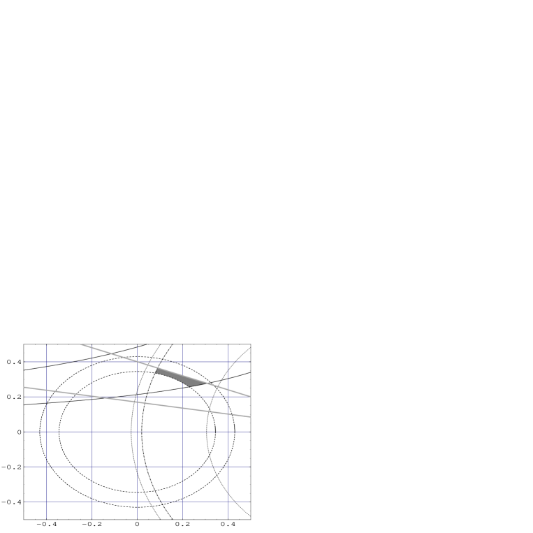
$\rho$

FIG. 1.: Determination of the apex $(\rho,\eta)$ of the unitarity triangle: The grey area is the presently allowed region, which is determined by (a) the measurement of $|V_{ub}/V_{cb}|$ (dashed circles), (b) the observed $B_{d}^{0}-\bar{B}_{d}^{0}$ mixing parameter $\Delta m_{d}$ (dotted circles), (c) the lower bound on the $B_{s}^{0}-\bar{B}_{s}^{0}$ mixing parameter $\Delta m_{s}$ (dashed-dotted circle), (d) the measurement of $\varepsilon_{K}$ (solid hyperbolae) and (e) the combined result of the CDF, BELLE and BaBar measurements of $a_{\psi K_{S}}$ (thick grey lines).

$\eta$

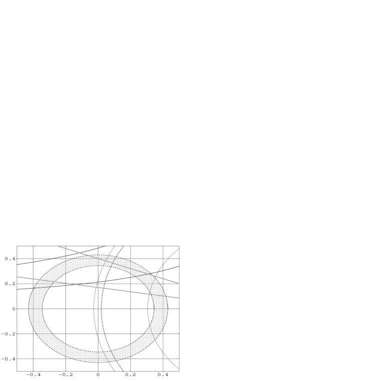
$\rho$

FIG. 2.: The shaded area corresponds to the allowed region in the $\rho-\eta$ plane for scenario (a). It is constrained solely by $R_{u}\in[0.34,~{}0.43]$, which is determined by the measurement of $|V_{ub}/V_{cb}|$ (dashed circles). For comparison we also show the other constraints appearing in Fig. 1, which are not relevant here.

$h$

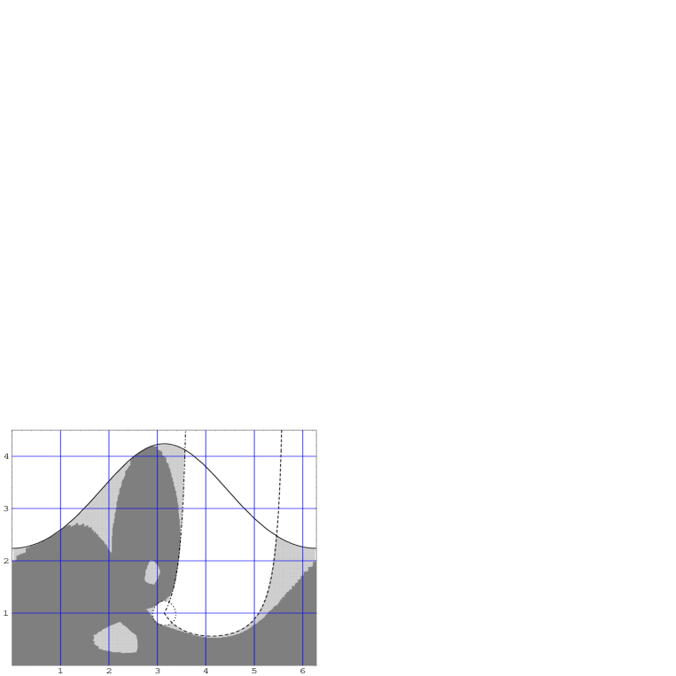
$\sigma$

FIG. 3.: The dark area corresponds to the allowed region in the $h-\sigma$ plane for scenario (a) according to our numerical analysis. It is embedded in the light area that results from the analytical boundaries based on the global constraints on $r_{d}$ from $\Delta m_{d,s}$ and $\theta_{d}$ from ${a_{\psi K_{S}}}$. Specifically the allowed range of $r_{d}$ excludes $h$ to be above $h^{max}_{r_{d}}(\sigma)$ (solid curve) or between $h^{\pm}_{r_{d}}(\sigma)$ (dotted curves), while the allowed range of $\theta_{d}$ exclude the region between $h^{min}_{\theta_{d}}(\sigma)$ (dashed curve) and $h^{max}_{\theta_{d}}(\sigma)$ (dashed-dotted curve). The numerical results are not much more constraining than the analytical ones, except for the “holes” in the dark regions that correspond to the excluded region within the $R_{u}$ annulus, which has been ignored in “global” analysis. (See appendix A 2 for details.)

$\eta$

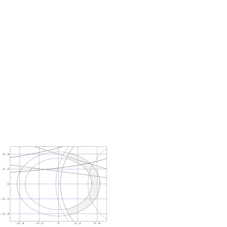
$\rho$

FIG. 4.: The shaded area corresponds to the allowed region in the $\rho-\eta$ plane for scenario (b). It is constrained by $R_{u}\in[0.34,~{}0.43]$ (dashed circles) and $\Delta m_{s}/\Delta m_{b}$ (dashed-dotted circle). For comparison we also show the other constraints appearing in Fig. 1, which are not relevant here.

$h$

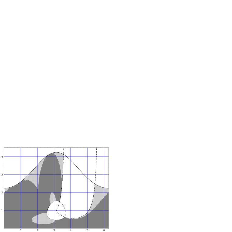
$\sigma$

FIG. 5.: The dark area corresponds to the allowed region in the $h-\sigma$ plane for scenario (b) according to our numerical analysis. It is embedded in the light area that results from the analytical boundaries based on the global constraints on $r_{d}$ from $\Delta m_{d,s}$ and $\theta_{d}$ from ${a_{\psi K_{S}}}$. Specifically the allowed range of $r_{d}$ excludes $h$ to be above $h^{max}_{r_{d}}(\sigma)$ (solid curve) or between $h^{\pm}_{r_{d}}(\sigma)$ (dotted curves), while the allowed range of $\theta_{d}$ excludes the region between $h^{min}_{\theta_{d}}(\sigma)$ (dashed curve) and $h^{max}_{\theta_{d}}(\sigma)$ (dashed-dotted curve). Due to the stronger bound on $r_{d}^{min}$ in scenario (b) the excluded area from $h^{\pm}_{r_{d}}(\sigma)$ is larger than in Fig. 3. (See appendix A 2 for details.)

$\eta$

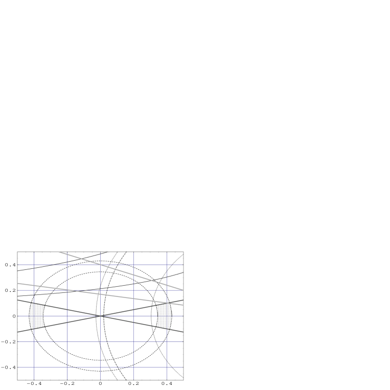
$\rho$

FIG. 6.: The shaded area corresponds to the allowed region in the $\rho-\eta$ plane for scenario (c). It is constrained by $R_{u}\in[0.34,~{}0.43]$ (dashed circles) and $\tan\delta_{KM}<0.25$ (“small phase”). For comparison we also show the other constraints appearing in Fig. 1, which are not relevant here.

$h$

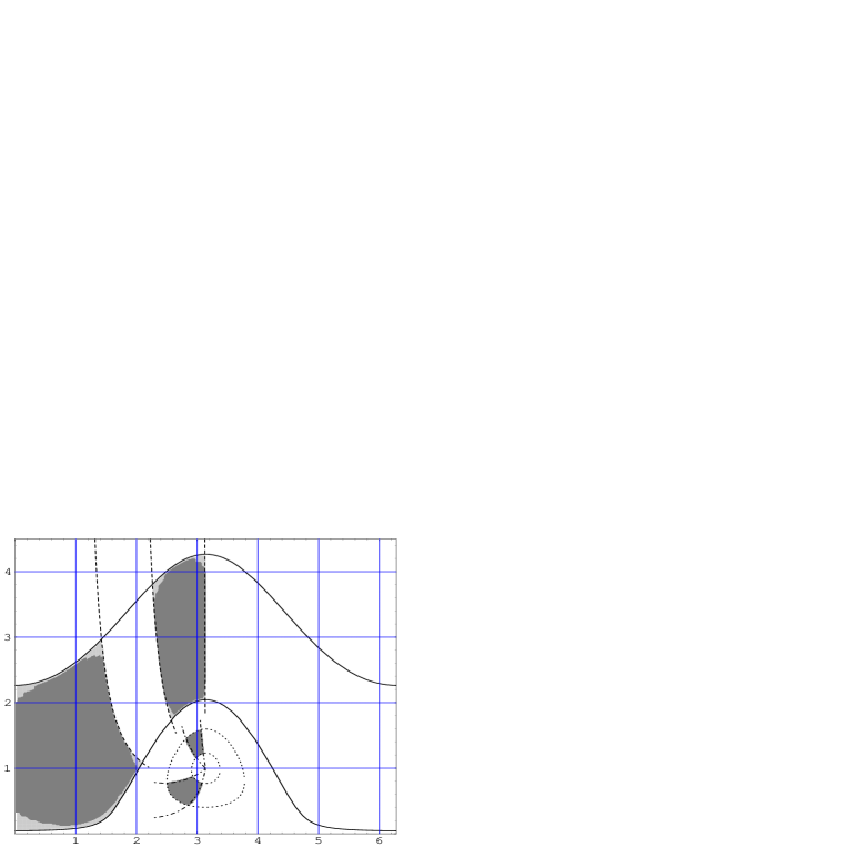
$\sigma$

FIG. 7.: The dark area corresponds to the allowed region in the $h-\sigma$ plane for scenario (c) according to our numerical analysis. It is embedded in the light area that results from the analytical boundaries based on the global constraints on $r_{d}$ from $\Delta m_{d,s}$ and $\theta_{d}$ from ${a_{\psi K_{S}}}$. Specifically there are two possible intervals for $r_{d}$, one corresponding to the large band between the solid curves for positive $\rho$ and one corresponding to the area between the dotted curves for negative $\rho$. The allowed ranges of $\theta_{d}$ limit the allowed region to be between the dashed ($\rho>0$) and dashed-dotted curves ($\rho<0$). Note that unlike for scenarios (a) and (b) in scenario (c) $h$ has a lower bound and $\sigma$ has an upper bound. (See appendix A 2 for details.)

$\eta$

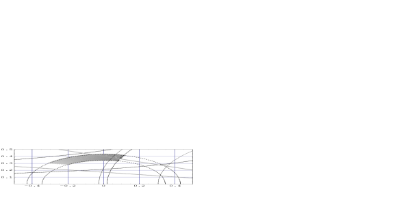
$\rho$

FIG. 8.: The shaded area corresponds to the “first” solution resulting from eqs. (4), (30) and (31) within models of MFV. The grey scale indicates the magnitude of $F_{tt}$ as a function of $\rho$ and $\eta$: The lightest region corresponds to $F_{tt}\simeq 0.4$ and the darkest region corresponds to $F_{tt}\simeq 2.7$. Adding the constraint from $\Delta m_{s}/\Delta m_{b}$ (dashed-dotted circle) practically the entire solution presented in this figure is excluded.

$\eta$

$\rho$

FIG. 9.: The shaded area corresponds to the allowed region according to the “second” solution resulting from eqs. (4), (30) and (31) within models of MFV. The grey scale indicates the magnitude of $F_{tt}$ as a function of $\rho$ and $\eta$: The lightest region corresponds to $F_{tt}\simeq 1.2$ and the darkest region corresponds to $F_{tt}\simeq 5.7$.

REFERENCES

- [1] D.E. Groom et al., Eur. Phys. J. C 15, (2000) 1.
-
[2]
N. Cabibbo, Phys. Rev. Lett. 10 (1963) 531;
M. Kobayashi and K. Maskawa, Prog. Th. Phys. 49 (1973) 652. - [3] R. Forty et al., ALEPH Collaboration, preprint ALEPH 99-099.
- [4] BaBar collaboration, hep-ex/0102030.
- [5] BELLE collaboration, hep-ex/0102018.
-
[6]
T. Affolder et al., CDF Collaboration,
Phys. Rev. D 61 (2000) 072005
[hep-ex/9909003]. -
[7]
K. Ackerstaff et al., OPAL Collaboration,
Eur. Phys. J. C 5 (1998) 379
[hep-ex/9801022]. - [8] L. Wolfenstein, Phys. Rev. Lett. 51 (1983) 1945.
-
[9]
The BaBar physics book (SLAC–R–504), Chapter 14,
available at:
http://www.slac.stanford.edu/pubs/slacreports/slac-r-504.html . - [10] A.J. Buras, hep-ph/0101336.
- [11] M. Ciuchini et. al., hep-ph/0012308.
- [12] Y-L. Wu, Y-F. Zhou, hep-ph/0102310.
- [13] D. Atwood and A. Soni, hep-ph/0103197.
-
[14]
S. Plaszczynski and M.-H. Schune, hep-ph/9911280;
Y. Grossman, Y. Nir, S. Plaszczynski and M.H Schune, Nucl. Phys. B 511 (1998) 69
[hep-ph/9709288]. - [15] G. Barenboim, G. Eyal and Y. Nir, Phys. Rev. Lett. 83 (1999) 4486 [hep-ph/9905397].
- [16] G. Eyal, Y. Nir and G. Perez, JHEP 0008 (2000) 028 [hep-ph/0008009].
-
[17]
Y. Nir and D. Silverman, Nucl. Phys. B 345 (1990) 301;
C.O. Dib, D. London and Y. Nir, Int. J. Mod. Phys. A6 (1991) 1253;
J.M. Soares and L. Wolfenstein, Phys. Rev. D 47 (1993) 1021;
Y. Nir, Phys. Lett. B 327 (1994) 85 [hep-ph/9402348];
Y. Grossman, Phys. Lett. B 380 (1996) 99 [hep-ph/9603244];
N.G. Deshpande, B. Dutta and S. Oh, Phys. Rev. Lett. 77 (1996) 4499
[hep-ph/9608231];
J.P. Silva and L. Wolfenstein, Phys. Rev. D 55 (1997) 5331 [hep-ph/9610208];
A.G. Cohen, D.B. Kaplan, F. Lepeintre and A.E. Nelson, Phys. Rev. Lett. 78 (1997) 2300 [hep-ph/9610252];
G. Barenboim, F.J. Botella, G.C. Branco and O. Vives, Phys. Lett. B 422 (1998) 277 [hep-ph/9709369]. - [18] A.J. Buras, P. Gambino, M. Gorbahn, S. Jager and L. Silvestrini, Phys. Lett. B 500 (2001) 161 [hep-ph/0007085].
- [19] A. J. Buras, P. Gambino, M. Gorbahn, S. Jager and L. Silvestrini, Nucl. Phys. B592 (2001) 55 [hep-ph/0007313].
- [20] E. Gabrielli and G.F. Giudice, Nucl. Phys. B 433 (1995) 3; Erratum Nucl. Phys. B 507 (1997) 549 [hep-lat/9407029].
-
[21]
G. Ecker and W. Grimus, D. Chang, Nucl. Phys. B 258 (1985) 328;
Z. Phys. C30 (1986) 293;
D. Chang, Nucl. Phys. B 214 (1983) 435. -
[22]
G. Barenboim, J. Bernabeu and M. Raidal,
Nucl. Phys. B478 (1996) 527
[hep-ph/9608450]. - [23] G. Barenboim et. al., Nucl. Phys. B511 (1998) 577 [hep-ph/9611347].
-
[24]
G. Barenboim, J. Bernabeu and M. Raidal,
Phys. Rev. D 55 (1997) 4213
[hep-ph/9702337]. -
[25]
G. Barenboim, J. Bernabeu, J. Matias and M. Raidal
Phys. Rev. D60 (1999) 016003
[hep-ph/9901265]. - [26] J.M. Frere et. al. Phys. Rev. D 46 (1992) 337.
- [27] P. Ball, J.M. Frere and J. Matias, Nucl. Phys. B 572 (2000) 3 [hep-ph/9910211].
- [28] P. Ball and R. Fleischer, Phys. Lett. B 475 (2000) 111 [hep-ph/9912319].
-
[29]
J.P. Silva and L. Wolfenstein,
Phys. Rev. D 55 (1997) 5331 [hep-ph/9610208];
Y. Grossman, Y. Nir and M.P. Worah, Phys. Lett. B 407 (1997) 307
[hep-ph/9704287];
G. Eyal and Y. Nir, JHEP 09 (1999) 013 [hep-ph/9908296];
G.C. Branco, P.A. Parada, T. Morozumi and M.N. Rebelo, Phys. Rev. D 48 (1993) 1167;
G.C. Branco, P.A. Parada, T. Morozumi and M.N. Rebelo, Nucl. Phys. Proc. Suppl. 37A (1994) 29. - [30] A.J. Buras and R. Buras, Phys. Lett. B 501 (2001) 223 [hep-ph/0008273].
-
[31]
A.J. Buras, M.E. Lautenbacher and G. Ostermaier,
Phys. Rev. D 50 (1994) 3433
[hep-ph/9403384]. - [32] T. Inami and C.S. Lim, Prog. Theor. Phys. 65 (1981) 297.
- [33] G.C. Branco, L. Lavoura and J.P. Silva, CP Violation, Clarendon-Oxford Press (1999) 188.
- [34] L.L. Chau and W.Y. Keung, Phys. Rev. Lett. 53, (1984) 1802.
-
[35]
V. Fanti et. al., Phys. Lett. B 465 (1999) 335;
T. Gershon, [hep-ph/0101034]. - [36] S. Adler et. al. E787 Collaboration, Phys. Rev. Lett. 84 (2000) 3768 [hep-ex/0002015].
- [37] ALEPH Collaboration, hep-ex/0010022.
-
[38]
H. Fusaoka and Y. Koide, Phys. Rev. D 57 (1998) 3986 [hep-ph/9712201];
M. Carena et. al., hep-ph/0010338.