TUM-HEP-656/07

MADPH-07-1478

New features in the simulation of neutrino oscillation experiments with GLoBES 3.0

(General Long Baseline Experiment Simulator)

Patrick Huber,  Joachim Kopp,  Manfred Lindner,
Mark Rolinec,  Walter Winter

Department of Physics, University of Wisconsin,

1150 University Avenue, Madison, WI 53706, USA

Max–Planck–Institut für Kernphysik,

Postfach 10 39 80, D–69029 Heidelberg, Germany

Physik–Department, Technische Universität München,

James–Franck–Strasse, 85748 Garching, Germany

Universität Würzburg, Institut für theoretische Physik und Astrophysik,

Am Hubland, D-97074 Würzburg, Germany

We present Version 3.0 of the GLoBES (“General Long Baseline Experiment Simulator”) software, which is a simulation tool for short- and long-baseline neutrino oscillation experiments. As a new feature, GLoBES 3.0 allows for user-defined systematical errors, which can also be used to simulate experiments with multiple discrete sources and detectors. In addition, the combination with external information, such as from different experiment classes, is simplified. As far as the probability calculation is concerned, GLoBES now provides an interface for the inclusion of non-standard physics without re-compilation of the software. The set of experiment prototypes coming with GLoBES has been updated. For example, built-in fluxes are now provided for the simulation of beta beams.

PACS: 14.60.Pq

Keywords: Neutrino oscillations, Long-baseline experiments, GLoBES

1 Introduction

Neutrino oscillations are now established as the leading flavor transition mechanism for neutrinos in a long history of many experiments, see e.g. Ref. [1] and references therein. Future facilities, using accelerator-based neutrino beams or nuclear reactors as neutrino sources, are proposed for precision measurements of the neutrino oscillation parameters. In the simulation of these experiments, the presence of multiple solutions which are intrinsic to neutrino oscillation probabilities [2, 3, 4, 5] affect the performance. Thus, optimization strategies are required which maximally exploit complementarity between experiments. The GLoBES software package [6] is a modern experiment simulation and analysis tool for a highly accurate beam and detector simulation. In addition, it provides powerful means to analyze correlations and degeneracies, especially for the combination of several experiments. Compared to a Monte Carlo simulation, which yields a different result in each run, it simulates the performance of the average experiment (see Ref. [7] for a discussion of the meaning of “average”). The advantage of such an average prediction is a tremendous performance gain, which can be used for systematical parameter space scans. In addition, it simplifies the direct comparison of experiments.

The GLoBES software has, in the past, been used for many studies, some of them are referred to in the paper. However, recent developments have indicated that extensions and improvements are necessary. In this work, we present the most important new features and changes in GLoBES 3.0. For experimentalists, GLoBES now allows for the implementation of arbitrary systematics, which can also be used for the simulation of multi-detector experiments. In addition, several extensions have been included in AEDL (“Abstract Experiment Description Language”), such as built-in beta beam fluxes and the possibility to use lists as variables. For phenomenologists, user-defined priors provide a flexible interface to include external information, such as from different experiments. In addition, GLoBES now can be used for the simulation of non-standard physics without re-compiling the GLoBES software.

2 Concept of GLoBES

GLoBES (“General Long Baseline Experiment Simulator”) is a flexible software tool to simulate and analyze neutrino oscillation short- and long-baseline experiments using a complete three-flavor description. On the one hand, it contains a comprehensive abstract experiment definition language (AEDL), which allows to describe most classes of long baseline and reactor experiments at an abstract level. On the other hand, it provides a C-library to process the experiment information in order to obtain oscillation probabilities, rate vectors, and $\Delta\chi^{2}$-values (cf., Fig. 1). In addition, it provides a binary program to test experiment definitions very quickly, before they are used by the application software. Currently, GLoBES is available for GNU/Linux.

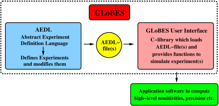
Figure 1: General concept of the GLoBES package.

GLoBES allows to simulate experiments with stationary neutrino point sources, where each experiment is assumed to have only one neutrino source. Such experiments are neutrino beam experiments and reactor experiments. Geometrical effects of a continuous source distribution, such as in the sun or the atmosphere, can not be described. In addition, sources with a physically significant time dependence can not be studied, such as supernovæ. However, in GLoBES 3.0 and higher, new flexibility is introduced by the concept of user-defined systematics. This new feature allows the cross-definition of systematical errors over different experiments. In principle, this mechanism can be used for the combination of several discrete sources and one detector, or several detectors and one source, or several sources and several detectors. In addition, already implemented concepts of GLoBES have been used for indirect simulations of geometrical effects. For example, the mapping of the detector location on the neutrino energy has been simulated in Ref. [8] by the use of variable bin widths.

On the experiment definition side, either built-in neutrino fluxes (e.g., neutrino factory, beta beam) or arbitrary, user-defined fluxes can be used. Similarly, arbitrary cross sections, energy dependent efficiencies, energy resolution functions as well as the considered oscillation channels, backgrounds, and many other properties can be specified. For the systematics, energy normalization and calibration errors can be simulated, or the systematics can be completely user-defined. Note that energy ranges and windows and bin widths can be (almost) arbitrarily chosen, including bins of different widths. Together with GLoBES comes a number of pre-defined experiments in order to demonstrate the capabilities of GLoBES and to provide prototypes for new experiments. In addition, they can be used to test new physics ideas with complete experiment simulations.

With the C-library, one can extract the $\Delta\chi^{2}$ for all defined oscillation channels for an experiment or any combination of experiments. Of course, also low-level information, such as oscillation probabilities or event rates, can be obtained. GLoBES includes the simulation of neutrino oscillations in matter with arbitrary matter density profiles. In addition, it allows to simulate the matter density uncertainty (see, e.g., Refs. [9, 10]) and to extract the precision on the matter density (see, e.g., Refs. [11, 12]). As one of the most advanced features of GLoBES, it provides the technology to project the $\Delta\chi^{2}$, which is a function of all oscillation parameters, onto any subspace of parameters by local minimization. This approach allows the inclusion of multi-parameter-correlations, where external constraints (e.g., on the solar parameters) can be imposed, too. Applications of the projection mechanism include the projections onto the $\sin^{2}2\theta_{13}$-axis and the $\sin^{2}2\theta_{13}$-$\delta_{\mathrm{CP}}$-plane. In addition, all oscillation parameters can be kept free to numerically localize degenerate solutions.

3 Oscillation probabilities and the simulation of non-standard physics

The probability calculation in GLoBES is based on the diagonalization of the Hamiltonian in layers of constant matter density using the standard three flavor scenario of neutrino oscillations. In the flavor base, we have

$$\mathcal{H}(n_{e})=\frac{1}{2E}\,U\,\left(\begin{array}[]{ccc}0&0&0\\ 0&\Delta m_{21}^{2}&0\\ 0&0&\Delta m_{31}^{2}\\ \end{array}\right)\,U^{\dagger}+\left(\begin{array}[]{ccc}\pm\sqrt{2}G_{F}n_{e}&0&0\\ 0&0&0\\ 0&0&0\end{array}\right)$$ (1)

with $U$ being the mixing matrix (described by four parameters $\theta_{12}$, $\theta_{13}$, $\theta_{23}$, and $\delta_{\mathrm{CP}}$), and $n_{e}$ the constant electron density in the respective matter density layer. The electron density is related to the matter density $\rho$ by $n_{e}\simeq 0.5\,\rho/m_{N}$ with $m_{N}$ being the nucleon mass. The sign in the second term depends on whether one uses neutrinos or antineutrinos. For $k$ matter density layers with densities $n^{k}_{e}$ and thicknesses $x_{i}$, the oscillation probability then evaluates to

$$P(\nu_{\alpha}\rightarrow\nu_{\beta})=\left|\langle\nu_{\beta}|\mathcal{E}(n^{k}_{e},x_{k})\ldots\mathcal{E}(n^{1}_{e},x_{1})|\nu_{\alpha}\rangle\right|^{2}$$ (2)

with the evolution operators (see, e.g., Ref. [13])

$$\mathcal{E}(n^{k}_{e},x_{k})=\exp\left(-i\mathcal{H}(n^{k}_{e})x_{k}\right)=\frac{1}{2E}\,\hat{U}(n^{k}_{e})\,\left(\begin{array}[]{ccc}e^{-i\,m_{1}^{k}\,x_{k}}&0&0\\ 0&e^{-i\,m_{2}^{k}\,x_{k}}&0\\ 0&0&e^{-i\,m_{3}^{k}\,x_{k}}\end{array}\right)\,\hat{U}(n^{k}_{e})^{\dagger}\,.$$ (3)

Here the Hamiltonian $\mathcal{H}(n^{k}_{e})$ is diagonalized by the unitary mixing matrix in matter $\hat{U}(n^{k}_{e})$ with the eigenvalues $m_{1}^{k}$, $m_{2}^{k}$, and $m_{3}^{k}$. The probabilities in Eq. (2) are used for the event rate computation, which is described in greater detail in Ref. [6]. In the next section, we will demonstrate how systematics is implemented.

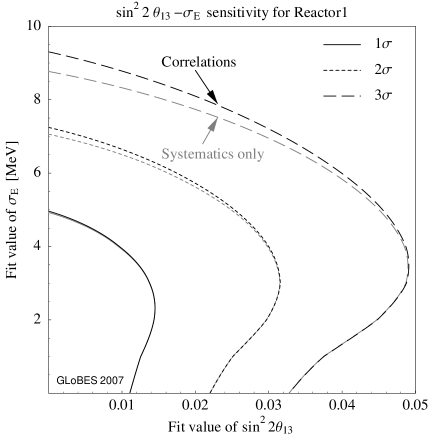
Figure 2: Fit in the $\sin^{2}2\theta_{13}$-$\sigma_{E}$-plane for the simulated values $\sin^{2}2\theta_{13}=\sigma_{E}=0$ (figure similar to Ref. [14]). Here $\sigma_{E}$ is an additional non-standard parameter describing the wave packet width of the neutrino oscillation wave packet. If this parameter is kept free (vertical axis), the $\sin^{2}2\theta_{13}$ sensitivity (horizontal axis) will be affected. Note that the standard $\sin^{2}2\theta_{13}$ sensitivity is given by the curves for $\sigma_{E}\equiv 0$. The figure is computed with example6.c coming with the GLoBES 3.0 distribution (and higher).

GLoBES 3.0 allows the modification of this Hamiltonian and the whole probability engine without re-compilation of the GLoBES software. This is implemented by using pointers to the functions of the standard probability engine, which can be changed by registering a different probability engine. For example, a user may just copy the standard probability engine of GLoBES, modify it, and register it. An important prerequisite is the ability to handle more than the standard six oscillation parameters (plus matter density) $\boldsymbol{\lambda}=(\theta_{12},\theta_{13},\theta_{23},\delta_{\mathrm{CP}},\Delta m_{21}^{2},\Delta m_{31}^{2},\rho)$, i.e.,

$$\boldsymbol{\lambda}=(\theta_{12},\theta_{13},\theta_{23},\delta_{\mathrm{CP}},\Delta m_{21}^{2},\Delta m_{31}^{2},\rho,\eta_{1},\ldots,\eta_{n})$$ (4)

with $n$ non-standard parameters $\eta_{j}$. These parameters can be accessed in the usual way, see Ref. [15]. For example, non-standard Hamiltonian effects in the $e$-$\tau$-sector may be introduced by modifying Eq. (1) to

$$\mathcal{\hat{H}}=\mathcal{H}(n_{e})+\left(\begin{array}[]{ccc}0&0&\epsilon_{e\tau}\\ 0&0&0\\ \epsilon_{e\tau}^{*}&0&0\end{array}\right)$$ (5)

In this case, there are two more real parameters, such as the absolute value and phase of $\epsilon_{e\tau}$. In the literature, the non-standard physics feature in GLoBES as experimental feature has been used for damping effects (such as neutrino decoherence, decay, etc.) in Ref. [14], Hamiltonian-level effects (such as non-standard matter effects) in Ref. [16], and mass-varying neutrinos in Ref. [17] by implementing an environment dependence of neutrino mass. We show in Fig. 2 a result from Ref. [14] provided as example6.c in the GLoBES distribution. In this case, the non-standard physics is a loss of coherence in neutrino oscillations described by an intrinsic width of the mass eigenstate wave packets $\sigma_{E}$ (in energy space). Compared to Eq. (5), the underlying physics takes place at the probability level, i.e., Eq. (2), and it can be easily implemented analytically (for details, see Ref. [14]). In example6.c, an analytical implementation of this physics is used for simplicity.

4 Systematics implementation and user-defined systematics

GLoBES supports four types of systematical errors by default: Signal and background normalization errors, as well as signal and background tilt or energy calibration errors. The tilt (T) is implemented as a linear distortion of the spectrum around the center, and the energy calibration (C) as a distortion (stretching) of the reconstructed energy scale. For the implementation of these systematical errors, the “pull method” is used [18], which introduces so-called nuisance parameters $\zeta_{i}$. For example, for the signal and background normalization errors, the respective event rates $s_{i}$ and $b_{i}$ in each bin $i$ are multiplied with

$$s_{i}(\zeta_{1}):=(1+\zeta_{1})\cdot s_{i}\,,\quad b_{i}(\zeta_{2}):=(1+\zeta_{2})\cdot b_{i}\,,$$ (6)

i.e., the rates are scaled by these parameters. The systematics $\chi^{2}$ is then minimized over these parameters:

$$\chi^{2}_{\mathrm{pull}}(\boldsymbol{\lambda}):=\min_{\{\zeta_{i}\}}\,\,\left(\,\chi^{2}(\boldsymbol{\lambda},\zeta_{1},\ldots,\zeta_{k})+\sum_{j=1}^{k}\frac{\zeta_{j}^{2}}{\sigma_{\zeta_{j}}^{2}}\,\right)\,.$$ (7)

Here $\chi^{2}(\boldsymbol{\lambda},\zeta_{1},\ldots,\zeta_{k})$ is the usual Possonian $\chi^{2}$ depending on the neutrino oscillation parameters $\boldsymbol{\lambda}$ and the nuisance parameters $\zeta_{i}$ (which, for instance, scale the signal or background rates). In addition, Gaussian penalties $\zeta_{j}^{2}/\sigma_{\zeta_{j}}^{2}$ are added, where $\sigma_{\zeta_{j}}$ corresponds to the actual systematical error. The core part of Eq. (7) is the definition of $\chi^{2}$. For example, for a background-free measurement and a signal normalization error only, it reads

$$\chi^{2}(\boldsymbol{\lambda},a)=\sum_{i=1}^{\textrm{\# of bins}}2\left((1+a)T_{i}-O_{i}+O_{i}\log\frac{O_{i}}{(1+a)T_{i}}\right)+\frac{a^{2}}{\sigma_{a}^{2}}\,,$$ (8)

where $O_{i}$ are the observed rates (corresponding to the data or true values), and $T_{i}$ are the theoretical (fit) rates. Let us assume that we have two detectors, such as for a reactor experiment with a near and far detector. Using standard systematics in GLoBES, one has

$$\chi^{2}_{\mathrm{pull}}(\boldsymbol{\lambda})=\min_{a}\,\,\left(\,\chi_{1}^{2}(\boldsymbol{\lambda},a)+\frac{a^{2}}{\sigma_{a}^{2}}\,\right)+\min_{b}\,\,\left(\,\chi_{2}^{2}(\boldsymbol{\lambda},b)+\frac{b^{2}}{\sigma_{b}^{2}}\,\right)\,.$$ (9)

In this case, the normalization between the two detectors will be uncorrelated.

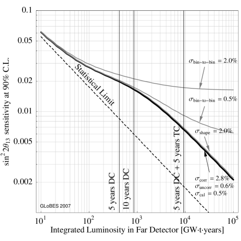
Figure 3: Luminosity scaling of the $\sin^{2}2\theta_{13}$ sensitivity for different systematical error assumptions (90% confidence level, figure similar to Ref. [19]). The thick curve corresponds to Eq. (10) for $\sigma_{R}=\sigma_{\mathrm{corr}}=2.8\%$, $\sigma_{N}=\sigma_{F}=\sigma_{\mathrm{uncorr}}=0.6\%$ and an additional calibration error. The figure is computed with example5.c provided with the GLoBES software.

Using GLoBES 3.0 and higher, one can modify the standard $\chi^{2}$ function in GLoBES which corresponds to Eq. (8). In addition, the systematics concept of “error dimensions” is replaced by a concept directly related to this $\chi^{2}$ function. As an example, consider a reactor experiment with near ($N$) and far ($F$) detectors which are described by a reactor flux uncertainty $\sigma_{R}$ and two fiducial volume errors of the near $\sigma_{N}$ and far $\sigma_{F}$ detectors. Then Eq. (8) will be replaced by

$$\chi^{2}(\boldsymbol{\lambda},a_{N},a_{F},a_{R})= \sum_{i=1}^{\textrm{\# of bins}}\sum_{d=N,F}2\Big{(}(1+a_{R}+a_{d})T_{d,i}-O_{d,i}+$$

$$\left.+O_{d,i}\log\frac{O_{d,i}}{(1+a_{R}+a_{d})T_{d,i}}\right)+\frac{a_{R}^{2}}{\sigma_{R}^{2}}+\frac{a_{N}^{2}}{\sigma_{N}^{2}}+\frac{a_{F}^{2}}{\sigma_{F}^{2}}$$ (10)

This function can be defined with user-defined systematics. Similarly, calibration errors, shape errors, uncorrelated bin-to-bin errors, etc., can be introduced. We show in Fig. 3 the result of such a calculation, where the thick curve corresponds to Eq. (10) plus an additional energy calibration error. Furthermore, more complicated setups using multiple discrete sources and detectors can be simulated. For details, we refer to the manual [15]. In the past, user-defined systematics has (as experimental feature) been used in Ref. [19] to simulate Double Chooz, in Ref. [20] to simulate T2KK, and in Ref. [21] to simulate various reactor experiment setups and complicated backgrounds from geoneutrinos.

In summary, GLoBES currently supports the following systematics $\chi^{2}$ functions:

chiSpectrumTilt

Spectral information, signal and background normalization errors and tilts

chiNoSysSpectrum

No systematical errors, but spectral information

chiTotalRatesTilt

Total rates only, signal and background normalization errors and tilts

chiSpectrumOnly

Spectrum only (free signal normalization), no other systematics

chiNoSysTotalRates

Total rates only, no systematics

chiSpectrumCalib

Spectral information, signal and background normalization errors and energy calibration errors

chiZero

Passive systematics (returns $\chi^{2}=0$, only provides the event rates for the access by other rules or experiments)

Any other name

User-defined systematics

5 Adding external information with user-defined priors

In order to include correlations and degeneracies, GLoBES provides (local) marginalization routines to project the fit manifold onto a subspace. For example, if one wants to compute the $\sin^{2}2\theta_{13}$ precision, one scans the $\sin^{2}2\theta_{13}$ direction and marginalizes for each fixed $\sin^{2}2\theta_{13}$ over the other oscillation parameters. This marginalization is performed after the systematics $\chi^{2}_{\mathrm{pull}}$ in Eq. (7) (or similar) has been determined:

$$\chi^{2}_{\mathrm{proj}}(\boldsymbol{\lambda_{1}}):=\min_{\{\boldsymbol{\lambda_{2}}\}}\left(\,\chi^{2}_{\mathrm{pull}}(\boldsymbol{\lambda_{1}},\boldsymbol{\lambda_{2}})\,\right)\,.$$ (11)

In this case, the parameter space of oscillation parameters $\boldsymbol{\lambda}$ is projected onto the subspace $\boldsymbol{\lambda_{1}}$. If one wants to include external input, which only depends on the oscillation parameters and not on systematics, one can do so at this level. GLoBES provides the pre-defined possibility to include external Gaussian constraints on the oscillation parameters (and the matter density, which is treated as another oscillation parameter). For example, an external constraint on $\theta_{12}$ is added before the marginalization in Eq. (11) by the replacement

$$\chi^{2}_{\mathrm{pull}}(\boldsymbol{\lambda})\rightarrow\chi^{2}_{\mathrm{pull}}(\boldsymbol{\lambda})+\frac{(\theta_{12}-\theta_{12}^{0})^{2}}{\sigma_{\theta_{12}}^{2}}$$ (12)

with the central value $\theta_{12}^{0}$, where the input is added, and the $1\sigma$ Gaussian error $\sigma_{\theta_{12}}$. This corresponds to an external measurement of the solar mixing angle at the best-fit value $\theta_{12}^{0}$ with the error $\sigma_{\theta_{12}}$.

In practice, the external error on $\theta_{12}$ may not be Gaussian or one may want to add other external information. Therefore, GLoBES 3.0 and higher provides the concept of user-defined priors $f(\boldsymbol{\lambda})$. Instead of Eq. (12), we then have

$$\chi^{2}_{\mathrm{pull}}(\boldsymbol{\lambda})\rightarrow\chi^{2}_{\mathrm{pull}}(\boldsymbol{\lambda})+f(\boldsymbol{\lambda})\,.$$ (13)

One can easily imagine that this simple concept allows for a high degree of freedom. Examples where this feature has been used as an experimental feature are the combination of terrestrial neutrino data with the information from neutrino telescopes [22] and the combination of long-baseline data with atmospheric neutrino data [23, 24]. Another very interesting option is the use of penalties in degeneracy localization, as suggested by Thomas Schwetz. For example, if the minimizer runs into the wrong octant, user-defined priors can be used to add a penalty and prevent it from doing so.

6 AEDL changes and experiment prototypes

Experiment	File name	Short description	Refs.
Superbeam experiments:
T2K	T2K.glb	J-PARC to Super-Kamiokande	[25, 9]
T2HK	T2HK.glb	J-PARC to Hyper-Kamiokande	[25, 9]
NO$\nu$A	NOvA.glb	Fermilab NuMI beamline off-axis	[26, 27]
SPL	SPL.glb	CERN to Fréjus	[24, 28, 29]
Reactor experiments:
Reactor-I	Reactor1.glb	Small reactor exp., $\mathcal{L}=400\,\mathrm{t}\,\mathrm{GW}\,\mathrm{yr}$	[30]
Reactor-II	Reactor2.glb	Large reactor exp., $\mathcal{L}=8\,000\,\mathrm{t}\,\mathrm{GW}\,\mathrm{yr}$	[30]
DoubleChooz	D-Chooz_near.glb	Double Chooz near detector	[19]
	D-Chooz_far.glb	Double Chooz far detector
Beta beams:
Low $\gamma$	BB_100.glb	$\gamma=100$ CERN to Fréjus scenario	[24]
Medium $\gamma$	BB_350.glb	$\gamma=350$ “refurbished SPS” scenario (or other accelerator)	[31]
Variable $\gamma$	BBvar_WC.glb	Variable $\gamma$ beta beam with water Cherenkov detector, $50\lesssim\gamma\lesssim 500$	[32]
	BBvar_TASD.glb	Variable $\gamma$ beta beam with totally active scint. detector (TASD), $100\lesssim\gamma\lesssim 3\,000$	[32]
Neutrino factories:
Standard	NFstandard.glb	Standard neutrino factory, $50\,\mathrm{kt}$ magnetized iron calorimeter, $E_{\mu}=50\,\mathrm{GeV}$	[9]
Variable $E_{\mu}$	NFvar.glb	Variable neutrino factory, disapp. channels without CID; $10\,\mathrm{GeV}\lesssim E_{\mu}\lesssim 80\,\mathrm{GeV}$	[9, 33]
Gold + Silver	NF_GoldSilver.glb	As NFvar.glb plus 5 kt ECC detector for Silver Channel measurement	[9, 33, 34]
Hybrid detector	NF_hR_lT.glb	As NFvar.glb, but lower threshold and better energy resolution	[9, 33]

Table 1: Pre-defined experiment prototypes coming with GLoBES 3.0: The columns represent the AEDL filename, a short description, and the references in which the files are originally used and discussed (except for minor modifications, such as a different implementation of the energy threshold function).

AEDL (Abstract Experiment Definition Language) is a special syntax developed for the description of experiments in GLoBES, represented by simple text files. Core part of AEDL are the following constructions (for details, see Ref. [15]):

Channel

A channel represents an oscillation channel from the source flux, over the initial and final flavors and the use of neutrinos or antineutrinos, to the interaction type and cross section. The result is an event rate vector.

Rule

A rule combines one or more signal channels with one or more background channels. The rates from these channels are added, and the signal and background are implemented with specific systematics, i.e., systematics is connected to the concept of a rule. The result of a rule is a systematics $\chi^{2}$ corresponding to Eq. (7).

Experiment

An experiment is a combination of one or more rules, which may correspond to different appearance and disappearance channels, neutrino and antineutrino operations modes, etc.. An experiment has a common detector and baseline, but may use several different fluxes (such as for neutrinos and antineutrinos). Therefore, the matter density profile is the same for all rules of an experiment. The result of an experiment is again a systematics $\chi^{2}$, but summed over all rules.

Experiment combination

An experiment combination consists of different experiments with different detectors, baselines, and (uncorrelated) matter density profiles. The result of an experiment combination is again a systematics $\chi^{2}$, but summed over all experiments.

Note that after the $\chi^{2}$ is summed over all rules or experiments as specified by the user in the application software, Eq. (11) is applied, and the oscillation parameters are marginalized over.

In GLoBES 3.0, this construction of experiments is extended by user-defined systematics, which allows the user to break up the strict coupling between systematics and rules. For example, systematics can be correlated between different rules or experiments, such as for a reactor experiment with identical near and far detectors. In addition, one can introduce user-defined systematical errors. For that purpose, the former error dimension concept has been changed and extended. For example, one has to give each user-defined systematics a name, and this name has to be matched by the application software. Further changes in AEDL are the requirement to specify the minimum GLoBES version the AEDL file can be used with, and the extensions by lists as AEDL variables and by an interpolation feature.

As far as the experiment prototypes are concerned, a list of the ones provided with GLoBES 3.0 is given in Table 1. These prototypes can be modified for the definition of one’s own experiments (experimentalist), or they can be used for the test of new physics concepts (phenomenologist/theorist). Note that some of these experiments may contain integrated luminosities, baseline, fluxes, efficiencies, or other factors, which the user may not agree with and which can be easily adjusted. Some of the AEDL files have been changed or updated from earlier versions, such as for T2K and T2HK, or the standard neutrino factory. Other files represent the results from recent developments, such as the variable energy beta beam or neutrino factory files. They push AEDL to the edge in terms of advanced features, such as variable bin widths, use of the new interpolation feature, threshold function implementations, etc.. In particular, note that Double Chooz requires user-defined systematics, and the beta beams require built-in beta beam fluxes. Both of these features are only available in GLoBES 3.0 and higher. Some of the files require that AEDL variables be pre-set by the user, such as the muon energy for the variable energy neutrino factory. These variables are described in the corresponding file headers. Old AEDL prototypes should still run, but will not be maintained by the GLoBES team anymore.

7 Internal changes and improved performance

Sophisticated GLoBES simulations with several experiments and complicated parameter correlations can take several days to finish even on modern computers. To mitigate this problem as far as possible, we have taken several steps to optimize the performance of the multi-dimensional minimizations, which are at the heart of each GLoBES $\chi^{2}$ analysis.

Firstly, the GLoBES minimizers distinguish between minimization over oscillation parameters and minimization over systematics (nuisance) parameters. This is necessary because each step in the oscillation parameter space requires a time-consuming re-computation of oscillation probabilities, while a modification of the systematics parameters does not. The standard procedure is to perform a full minimization in systematics space after each step in oscillation space. This avoids interference of the two categories of parameters, and is known to have excellent convergence properties. The numerical method that does the minimization is the Powell algorithm [35].

In GLoBES 3.0, we provide an alternative method, which does the full minimization in one go, and is therefore several times faster in most cases. In this algorithm, each Powell iteration over oscillation parameters is followed by one iteration over systematics parameters. Since there may be some pathological cases where this interleaved minimization strategy behaves differently than the old method, it is by default not used in GLoBES 3.0. This ensures maximal compatibility with old application programs, but it requires users who wish to benefit from the new algorithm to explicitly select it by an API function call.

Besides optimizing the minimization functions, it is also mandatory to optimize the routines which are called by them to calculate $\chi^{2}$ for one specific set of parameters. In particular, the computation of oscillation probabilities, which has to be done every time the oscillation parameters have changed, should be as efficient as possible. The most expensive step here is the diagonalization of the hermitian $3\times 3$ neutrino Hamilton operator in matter. The LAPACK routines [36], which were used to solve this eigenproblem in previous versions of GLoBES, turned out not to be the optimal choice because they are mainly optimized for very large matrices [37]. In the case of the small and usually well-conditioned matrices appearing in GLoBES, they spend too much time evaluating their parameter list and planning the optimal diagonalization strategy. Therefore, GLoBES now relies an algorithm which has been designed specifically for the diagonalization of hermitian $3\times 3$ matrices. It is essentially the extremely fast analytical algorithm discussed in Ref. [37], but for the rare cases where this may become inaccurate, it falls back to the QL method [38, 39].

As far as the installation of GLoBES on different systems is concerned, GLoBES has been improved in the past, such as to handle different Linux distributions. In addition, for high-throughput computing, GLoBES has been used or tested on 64 Bit systems, Condor clusters, and parallel clusters. An important prerequisite for the parallelization is the option to build static binaries, which is now illustrated in the examples. With these improvements, the performance of GLoBES has been pushed to the edge. Ref. [33] is probably the currently most demanding product of GLoBES, for which most of these features have been developed.

8 Summary and conclusions

We have presented GLoBES 3.0, which is a simulation software for future terrestrial neutrino oscillation facilities. GLoBES is now no further restricted to one source-one detector configurations, but it can simulate the systematics of arbitrary combinations of discrete sets of sources and detectors. In addition, user-defined systematical errors can be introduced. The new concept of user-defined priors allows the inclusion of external information at a different level. For example, constraints from atmospheric neutrino experiments or neutrino telescopes can be taken into account. In addition, they provide a powerful handle on complicated degeneracy localization. On the probability level, GLoBES now supports the simulation of non-standard physics beyond three-flavor neutrino oscillations without a re-compilation of the software. A very important prerequisite for this feature is the ability of GLoBES 3.0 to carry more than six oscillation parameters. New experiment prototypes make extensive use of these new features, as well as they are illustrated by examples in the manual. One prominent example is the Double Chooz experiment, which requires user-defined systematics to simulate correlated errors between the near and far detectors.

In conclusion, GLoBES 3.0 provides a number of new improvements, such as by including more flexibility. At the end, the developers of a software can never exactly foresee what the users are up for, and therefore flexible concepts allow for more space in problem realizations. In this version of GLoBES, three new such flexible concepts have been introduced: user-defined oscillation probabilities, user-defined systematics, and user-defined priors. These approaches will make an easy adjustment of the software possible for both experimentalists and theorists, and will allow for flexibility at all levels. Finally, note that the past has shown that there is often more than one possibility how a specific problem can be implemented in GLoBES.

Acknowledgments

For the current version of GLoBES, we would like to thank Thomas Schwetz, who has been pushing the software to the edge in the past few years. Furthermore, we would like to thank Tommy Ohlsson, Toshihiko Ota, and Julian Skrotzki for using and testing unpublished new features of the software. The development of GLoBES is currently being supported by the Emmy Noether-Program of Deutsche Forschungsgemeinschaft [WW]. In the past, the following institutions and organizations have supported members of the GLoBES team: Technische Universität München, Max-Planck-Institut für Physik, SFB 375 for astro-particle physics of Deutsche Forschungsgemeinschaft, Studienstiftung des Deutschen Volkes, Institute for Advanced Study, Princeton, W. M. Keck Foundation, and National Science Foundation.

References

- [1] V. Barger, D. Marfatia and K. Whisnant, Int. J. Mod. Phys. E12 (2003) 569, hep-ph/0308123, and references therein.
- [2] G.L. Fogli and E. Lisi, Phys. Rev. D54 (1996) 3667, hep-ph/9604415.
- [3] J. Burguet-Castell et al., Nucl. Phys. B608 (2001) 301, hep-ph/0103258.
- [4] H. Minakata and H. Nunokawa, JHEP 10 (2001) 001, hep-ph/0108085.
- [5] V. Barger, D. Marfatia and K. Whisnant, Phys. Rev. D65 (2002) 073023, hep-ph/0112119.
- [6] P. Huber, M. Lindner and W. Winter, Comput. Phys. Commun. 167 (2005) 195, hep-ph/0407333, http://www.mpi-hd.mpg.de/lin/globes/.
- [7] T. Schwetz, (2006), hep-ph/0612223.
- [8] M. Rolinec and J. Sato, (2006), hep-ph/0612148.
- [9] P. Huber, M. Lindner and W. Winter, Nucl. Phys. B645 (2002) 3, hep-ph/0204352.
- [10] T. Ohlsson and W. Winter, Phys. Rev. D68 (2003) 073007, hep-ph/0307178.
- [11] W. Winter, Phys. Rev. D72 (2005) 037302, hep-ph/0502097.
- [12] R. Gandhi and W. Winter, (2006), hep-ph/0612158.
- [13] T. Ohlsson and H. Snellman, Phys. Lett. B474 (2000) 153, hep-ph/9912295, Erratum ibidem B480, 419(E) (2000).
- [14] M. Blennow, T. Ohlsson and W. Winter, JHEP 06 (2005) 049, hep-ph/0502147.
-
[15]
GLoBES 3.0 User’s and experiment definition manual, 2007,
can be obtained at http://www.mpi-hd.mpg.de/lin/globes/. - [16] M. Blennow, T. Ohlsson and W. Winter, Eur. Phys. J. C (to be published), hep-ph/0508175.
- [17] T. Schwetz and W. Winter, Phys. Lett. B633 (2006) 557, hep-ph/0511177.
- [18] G.L. Fogli et al., Phys. Rev. D66 (2002) 053010, hep-ph/0206162.
- [19] P. Huber et al., JHEP 05 (2006) 072, hep-ph/0601266.
- [20] V. Barger et al., (2006), hep-ph/0610301.
- [21] J. Kopp et al., (2006), hep-ph/0606151.
- [22] W. Winter, Phys. Rev. D74 (2006) 033015, hep-ph/0604191.
- [23] P. Huber, M. Maltoni and T. Schwetz, Phys. Rev. D71 (2005) 053006, hep-ph/0501037.
- [24] J.E. Campagne et al., (2006), hep-ph/0603172.
- [25] Y. Itow et al., Nucl. Phys. Proc. Suppl. 111 (2001) 146, hep-ex/0106019.
- [26] NOvA, I. Ambats et al., (2004), hep-ex/0503053.
- [27] NOvA, T. Yang and S. Woijcicki, (2004), Off-Axis-Note-SIM-30.
- [28] J.E. Campagne and A. Cazes, Eur. Phys. J. C45 (2006) 643, hep-ex/0411062.
- [29] M. Mezzetto, J. Phys. G29 (2003) 1781, hep-ex/0302005.
- [30] P. Huber et al., Nucl. Phys. B665 (2003) 487, hep-ph/0303232.
- [31] J. Burguet-Castell et al., Nucl. Phys. B725 (2005) 306, hep-ph/0503021.
- [32] P. Huber et al., Phys. Rev. D73 (2006) 053002, hep-ph/0506237.
- [33] P. Huber et al., Phys. Rev. D74 (2006) 073003, hep-ph/0606119.
- [34] D. Autiero et al., hep-ph/0305185.
- [35] R. Fletcher and M.J.D. Powell, Comp. J. 6 (1963) 163.
- [36] E. Anderson et al., LAPACK Users’ Guide, Third ed. (Society for Industrial and Applied Mathematics, Philadelphia, PA, 1999).
- [37] J. Kopp, (2006), physics/0610206.
- [38] J.G.F. Francis, Comp. J. 4 (1961) 265.
- [39] J. Stoer and R. Bulirsch, Introduction to Numerical Analysis, Second ed. (Springer-Verlag, Berlin, Germany, 1993).