TUM-HEP-462/02

MPI-PhT/02-15

Superbeams versus Neutrino Factories^∗

P. Huber,  M. Lindner, and  W. Winter 

^,,Institut für theoretische Physik, Physik–Department, Technische Universität München,

James–Franck–Strasse, D–85748 Garching, Germany

Max-Planck-Institut für Physik, Postfach 401212, D–80805 München, Germany

Abstract

We compare the physics potential of planned superbeams with the one of neutrino factories. Therefore, the experimental setups as well as the most relevant uncertainties and errors are considered on the same footing as much as possible. We use an improved analysis including the full parameter correlations, as well as statistical, systematical, and degeneracy errors. Especially, degeneracies have so far not been taken into account in a numerical analysis. We furthermore include external input, such as improved knowledge of the solar oscillation parameters from the KamLAND experiment. This allows us to determine the limiting uncertainties in all cases. For a specific comparison, we choose two representatives of each class: For the superbeam, we take the first conceivable setup, namely the JHF to SuperKamiokande experiment, as well as, on a longer time scale, the JHF to HyperKamiokande experiment. For the neutrino factory, we choose an initially conceivable setup and an advanced machine. We determine the potential to measure the small mixing angle $\sin^{2}2\theta_{13}$, the sign of $\Delta m^{2}_{31}$, and the leptonic CP phase $\delta_{\mathrm{CP}}$, which also implies that we compare the limitations of the different setups. We find interesting results, such as the complete loss of the sensitivity to the sign of $\Delta m^{2}_{31}$ due to degeneracies in many cases.

1 Introduction

Atmospheric neutrino oscillations are now well established and imply for energies of some $\mathrm{GeV}$ neutrino oscillations on scales of about $100$ to $10,000\,\mathrm{km}$. The combination of all available data strongly favors the LMA solution for solar oscillations, which allows a sizable leptonic CP violation in long baseline oscillations. So–called neutrino factories are therefore very promising for precise measurements of the neutrino mass squared differences, the mixing angles, and the leptonic CP violation. The physics potential of neutrino factories has been studied for different setups, such as in Refs. [1, 2, 3, 4, 5, 6, 7, 8, 9, 10, 11, 12]. However, there are still technological challenges to be solved, which means that the first neutrino factory can not be expected to be completed within this decade. Until then, upgraded conventional beams, so–called superbeams, can be used as alternative neutrino sources, especially since much of their technology is anyway needed for neutrino factories. The physics potential of superbeams has, for example, been investigated in Refs. [13, 14, 15, 16, 17]. Thus, superbeams are the next logical step in staging scenarios towards neutrino factories. However, one may wonder where the physics potential of superbeams ends and if they could make neutrino factories obsolete. It is very hard to compare superbeams and neutrino factories on the basis of the specific studies above, because numerous setups and simplifications have been used and different levels of sophistication were employed, which means that it is not clear how these options can be compared when all effects are included and the same methods are applied. The aim of this paper is to study these two options in a comparative way and to demonstrate that, at least for the case of the LMA solution, neutrino factories are required for high precision measurements. Since the leading oscillation parameters can in all cases be determined with a very good precision, we focus on the most difficult parameters to measure in our comparison, which are $\sin^{2}2\theta_{13}$, $\mathrm{sgn}(\Delta m_{31}^{2})$, and $\delta_{\mathrm{CP}}$.

As mentioned above, an important issue in the comparison of superbeams and neutrino factories is the use of reasonable and comparable parameters. It does, for example, not make much sense to compare 20 years of running of a very sophisticated JHF to HyperKamiokande experiment with an initial stage neutrino factory running only for one year. We therefore define scenarios with comparable running times and similar sophistication within the respective framework. Specifically, we choose the following reference scenarios: First of all, the JHF to SuperKamiokande experiment (to be called JHF-SK) with a $2^{\circ}$ off–axis beam represents the initial stage superbeam. Its neutrino factory counterpart (labeled NuFact-I) is chosen to have an equal running time with a moderate number of stored muons. In addition, we take, as an advanced stage superbeam experiment, the JHF to HyperKamiokande experiment (named JHF-HK), again with a $2^{\circ}$ off–axis beam, compared to an advanced neutrino factory (NuFact-II) with equal running time and a large number of stored muons. The ranges defined by JHF-SK to JHF-HK and NuFact-I to NuFact-II cover the conceivable experimental setups, which means that any superbeam or neutrino factory experiment similar to ours can be expected to be found within these ranges. Whenever applicable, we will therefore show the results of the different scenarios in one plot to allow visual interpolation. Our results are based on a combined event rate analysis of all accessible oscillation channels with a statistical method which treats all parameters equally instead of arbitrarily selecting specific parameter subsets. This method was already applied in neutrino factory studies in Ref. [9] and it was very successful in finding any two–parameter correlation in the multi–dimensional parameter space. We use in this paper an improved version, which allows us to include even multi–parameter correlations. In addition, we include systematical errors, external input, and degeneracy problems.

The paper is organized as follows: First we motivate and define the used scenarios in Section 2. In Section 3, we introduce the different measurement errors which are included in our analysis. We then present in Section 4 the oscillation framework, which will allow us to understand most of the results analytically, followed by a discussion of oscillation parameter degeneracies in Section 5, which plays a major role in the analysis. In Sections 6 and 7 we then present our results, where we especially focus on the measurements of $\sin^{2}2\theta_{13}$ and $\delta_{\mathrm{CP}}$. In Section 8, we finally conclude with an overall comparison of the main results. Details of the event rate analysis and the used statistical methods are given in Appendices A, B, and C.

2 Long baseline oscillation experiments

Superbeams and neutrino factory beams have many things in common, but also have many differences in their setups. We therefore highlight the most important features and differences in this section.

2.1 Superbeams

Superbeams are based on conventional beam dump techniques for producing neutrino beams [18, 19, 20, 21]. An intense proton beam is typically directed onto a massive target producing mostly pions, which are captured by an optical system of magnets in order to obtain a pion beam. These pions decay in a decay pipe, yielding a muon neutrino beam. The neutrino beam, however, is contaminated by approximately $0.5\%$ of electron neutrinos. Reversing the electrical current in the lens system results in an antineutrino beam. The energy spectrum of the muon beam can be controlled over a wide range: it depends on the incident proton energy, the optical system, and the precise direction of the beam axis compared to the direction of the detector. It is possible to produce broad band high energy beams, such as the CNGS beam [18, 19], or narrow band lower energy beams, such as in some configurations of the NuMI beam [20].

Superbeams employ the same technique as conventional beams, but use a proton beam intensity closer to the mechanical stability limit of the target at a typical thermal power of $0.7\,\mathrm{MW}$ to $4\,\mathrm{MW}$. The much higher neutrino luminosity allows the use of the decay kinematics of pions to produce a so–called “off–axis beam”, where the detector is located some degrees off the main beam axis. This reduces the overall neutrino flux, but leads to an important relative suppression of the electron neutrino contamination. Several off–axis superbeams with energies of about $1\,\mathrm{GeV}$ to $2\,\mathrm{GeV}$ have been proposed in Japan [15, 22], America [23], and Europe [14, 24].

The most sensitive neutrino oscillation channel for the parameters we are interested in, is the $\nu_{\mu}\rightarrow\nu_{e}$ appearance channel. Therefore, the detector should have excellent capabilities to separate electron and muon charged current events. In addition, an efficient rejection of neutral current events is required, because the neutral current interaction mode is flavor blind. With low statistics, the magnitude of the contamination itself limits the sensitivity to the $\nu_{\mu}\rightarrow\nu_{e}$ transition severely, while with high statistics the insufficient knowledge of its magnitude constrains the sensitivity. A near detector allows, for example, a substantial reduction of the background uncertainty [15, 25] and plays a crucial role in controlling other systematical errors, such as the flux normalization, the spectral shape of the beam, and the neutrino cross section at low energies. At energies of about $1\,\mathrm{GeV}$, the dominant charge current interaction mode is quasi–elastic scattering, which suggests that the water Cherenkov detector is the optimal type of detector. At these energies, a baseline length of about $300\,\mathrm{km}$ would be optimal to measure at the first maximum of the oscillation. At about $2\,\mathrm{GeV}$, there is already a considerable contribution of inelastic scattering to the charged current interactions, which means that it would be useful to measure the energy of the hadronic part of the cross section. This favors low–Z hadron calorimeters, which also have a factor of ten better neutral current rejection capability compared to water Cherenkov detectors [23]. In this case, the optimum baseline is around $600\,\mathrm{km}$. The matter effects are expected to be small for these experiments for two reasons. First of all, an energy of about $1\,\mathrm{GeV}$ to $2\,\mathrm{GeV}$ is small compared to the MSW resonance energy of approximately $13\,\mathrm{GeV}$ in the upper mantle. The second reason is that the baseline is too short to build up significant matter effects.

2.2 Neutrino factories

At neutrino factories, decaying muons are stored in the long straight sections of a storage ring and are producing muon and electron anti neutrinos of equal numbers [26]. The muons are produced by pion decays, where the pions are produced by the same technique as for superbeams. After being collected, they have to be cooled and reaccelerated very quickly. This has not yet been demonstrated and is the major technological challenge for neutrino factories [27]. The spectrum and flavor content of the beam are completely characterized by the muon decay and are therefore very precisely known [28]. The only adjustable parameter is the muon energy $E_{\mu}$, which is usually considered to be at about $20$ to $50\,\mathrm{GeV}$. It is also possible to produce and store anti muons in order to obtain a CP–conjugated beam. The symmetric operation of both beams leads to the cancellation or drastical reduction of many errors and systematical effects. Unless otherwise stated, we will further on refer to the neutrino beam and leave it to the reader to CP–conjugate all quantities for the anti neutrino beam.

Amongst all flavors and interaction types, muon charged current events are the easiest to detect. The appearance channel with the best sensitivity therefore is the ${\bar{\nu}_{e}\rightarrow\bar{\nu}_{\mu}}$ transition, which produces so called “wrong sign muons”. Therefore, a detector must be able to identify the charge of a muon in order to distinguish appearance and disappearance channels. The dominant charge current interaction in the multi–GeV range is deep–inelastic scattering, making a good energy resolution for the hadronic energy deposition necessary. Magnetized iron calorimeters are thus the favored choice for neutrino factory detectors. In order to achieve the required muon charge separation, it is necessary to impose a minimum muon energy cut at at least $4\,\mathrm{GeV}$ [29]. This leads to a significant loss of neutrino events in the range of about $4\,\mathrm{GeV}$ to $20\,\mathrm{GeV}$, which means that a high muon energy of $E_{\mu}=50\,\mathrm{GeV}$ is desirable. The first oscillation maximum then lies at approximately $3\,000\,\mathrm{km}$. Matter effects are sizable at this baseline and energy and our limited knowledge of the Earth’s matter density profile is an additional source of errors.

2.3 Benchmark setups

For the comparison of superbeams and neutrino factories, we define benchmark setups. For each case we use an initial, low luminosity experiment and an advanced, high luminosity setup. For both superbeams and neutrino factories, we use in addition equal assumptions about target power and running time, since these factors are limited by similar technological and financial constraints.

As the prototype of a superbeam experiment, we choose the JHF–Kamioka neutrino project as described in Ref. [15], for which a detailed proposal is available. This experiment is the most advanced in planning and might be operational by 2007. Using the SuperKamiokande detector is also very attractive, since this detector has been operating for a long time and its performance is therefore well known. Furthermore, the proposed NuMI off–axis beam seems to be quite similar in its characteristics and physics reach [23]. Another argument to choose the JHF beam is that there exists an upgrade strategy both for beam and detector, which provides a straightforward choice for the advanced, high luminosity setup. Our benchmark setups are:

JHF-SK

is the initial, low luminosity version of the superbeam experiment. The target power is $0.75\,\mathrm{MW}$ and we assume a running period of 5 years with a neutrino beam. As detector, we use the SuperKamiokande detector with a fiducial mass of $22.5\,\mathrm{kt}$ and a baseline of $295\,\mathrm{km}$.

JHF-HK

is the advanced, high luminosity superbeam setup. The assumed target power is $4\,\mathrm{MW}$ and the assumed running period is 6 years with an anti neutrino beam and 2 years with a neutrino beam. As detector, we use the proposed HyperKamiokande detector with a fiducial mass of $1\,000\,\mathrm{kt}$ and a baseline length of $295\,\mathrm{km}$.

For the neutrino factories, we consider a parent muon energy of $E_{\mu}=50\,\mathrm{GeV}$ and a baseline of $3\,000\,\mathrm{km}$. Many studies indicate that this setup provides, in some sense, an optimal sensitivity to CP effects (for a summary, see [12]). Specifically, we define:

NuFact-I

is the initial, low luminosity version of a neutrino factory experiment with an assumed target power of $0.75\,\mathrm{MW}$, corresponding to $10^{20}$ useful muon decays per year [27]. The total running period is $5$ years, $2.5$ years of these with a neutrino beam and $2.5$ years of these with an anti neutrino beam. As detector, we use a magnetized iron calorimeter with a fiducial mass of $10\,\mathrm{kt}$.

NuFact-II

is the advanced, high luminosity neutrino factory setup with an assumed target power of $4\,\mathrm{MW}$, corresponding to $5.3\cdot 10^{20}$ useful muon decays per year [27]. Corresponding to the advanced superbeam, we assume a total running period of 8 years, 4 years of these with a neutrino beam and 4 years of these with an anti neutrino beam. As detector, we use a magnetized iron calorimeter with a fiducial mass of $50\,\mathrm{kt}$.

The luminosity increase from the initial to the advanced setup is for the JHF experiments approximately a factor of 95 and for the neutrino factory experiments roughly a factor of 42. The statistics of each setup can be inferred from Table 1, which shows the number of signal and background events in the appearance channel at $\sin^{2}2\theta_{13}=0.1$, which is the biggest value allowed by CHOOZ.

	JHF-SK	JHF-HK	NuFact-I	NuFact-II
Signal	139.0	13 180.0	1 522.8	64 932.6
Background	23.3	2 204.6	4.2	180.3
Total	162.3	15 384.6	1 527.0	65 113.0

Table 1: The number of appearance events for the setups defined in the text. The used oscillation parameters are ${\Delta m^{2}_{21}}=3.7\cdot 10^{-5}\,\mathrm{eV}^{2}$, $\sin^{2}2\theta_{12}=0.8$, ${\Delta m^{2}_{31}}=3\cdot 10^{-3}\,\mathrm{eV}^{2}$, $\sin^{2}2\theta_{23}=1$, $\sin^{2}2\theta_{13}=0.1$, and $\delta_{\mathrm{CP}}=0$.

2.4 Simulation of experiments

Precision measurements at long baseline neutrino experiments require a detailed understanding of the neutrino beam, the propagation of the neutrinos in matter, and the detection of the neutrinos. An evaluation of the physics potential must therefore model all involved aspects very accurately. Our analysis is based on event rates and adequate statistical methods, which are described in Appendices A, B, and C. The implementation, as it is used in this work, is described below:

Neutrino production

Each neutrino beam is characterized by the flux of each neutrino flavor as a function of the energy (see Figure 22). A superbeam is mostly composed of $\nu_{\mu}$, but also contains small contaminations (typically $<1\%$) of $\nu_{e}$, $\bar{\nu}_{\mu}$, and $\bar{\nu}_{e}$. The spectrum is dominated by the decay kinematics of pions and their initial momentum distribution, but K decays contribute as well, especially at higher energies. The pion and K meson productions are hadronic processes, for which the momentum distribution has to be determined by Monte–Carlo techniques. Superbeams may therefore be subject to considerable uncertainties [15, 30]. We include in our simulation the $\nu_{e}$ and $\bar{\nu}_{e}$ background of the beam and assign an uncertainty to both its magnitude (referred to as background normalization) and spectral shape (referred to as background tilt). Anti–muon neutrino beams can be produced by reversing the horn current, but the operation is not entirely symmetric. The two polarities of a superbeam are therefore considered to be essentially independent beams.

At a neutrino factory, the beam is produced by muon decay, i.e., for muons in the storage ring, by

$$\mu^{-}\rightarrow e^{-}+\nu_{\mu}+\bar{\nu}_{e}.$$

It thus consists of equal numbers of $\nu_{\mu}$ and $\bar{\nu}_{e}$ [26]. The kinematics of this decay process rests only on energy and momentum conservation and the beam of a neutrino factory can therefore be assumed to be exactly known in terms of the initial muon energy and flux. Compared to the superbeam, the machine can be operated symmetrically in both polarities. Therefore, the CP–conjugated beam, emerging from stored $\mu^{+}$ decays, can be assumed to be identical for the same energy and muon $\mu^{+}$ flux.

In general, we include reasonable uncertainties in the total flux normalizations and shapes for both types of experiments.

Neutrino propagation

The neutrino propagation is calculated by numerically solving the Schrödinger equation for three neutrino flavors in a constant (average) matter potential [6]. We treat all but the solar oscillation parameters as quantities which have to be determined by our experiments. This is a reasonable assumption, since the studied experiments lead to a significantly better precision of the leading oscillation parameter measurements than previous ones. The solar parameters, however, can not be measured very well and are therefore assumed to be constrained by the KamLAND experiment within the LMA region [31, 32]. Furthermore, since the appearance probability has been shown to depend only on the product ${\Delta m^{2}_{21}}\,\sin^{2}2\theta_{12}$ [33], we use this product as a fit parameter. For the matter density, we allow an uncertainty of about 5% [34] by treating it as an additional parameter.

Neutrino detection

The detection of neutrinos involves two main aspects: the neutrino interaction and the event detection. For the superbeams, we include the following interaction modes: $\nu_{\mu}$ charged current quasi–elastic scattering, $\nu_{\mu}$ and $\nu_{e}$ charged current inelastic scattering, and neutral current scattering for all flavors. For neutrino factories we only distinguish $\nu_{\mu}$ charged current events (quasi–elastic and inelastic scattering) and neutral current events for all flavors. The cross sections for all of these interactions are taken from Refs. [35, 36] and displayed in Figure 23. For the energies considered for neutrino factories, the cross sections can be assumed to be exactly known. However, at lower energies the cross sections may be subject to considerable hadronic uncertainties [37, 38]. We tested the influence of these uncertainties and found that, for the studied experiments, they are rather small.

The event detection introduces additional uncertainties, which are characterized by additional parameters. We include energy dependent detection efficiencies in order to take threshold effects and their errors into account and simulate the energy resolution by Gaussian averaging over adjacent bins. We also include flavor, charge, and event misidentification, leading, for example, to a certain fraction of neutral current events counted as charged current events and to another fraction of events detected with the wrong flavor. Thus, we include in addition to beam contaminations, backgrounds from event misidentification with uncertainties in magnitudes and spectral shapes. Further on, we will use the term “background” to refer to the sum of all influences leading to uncertainties in the overall normalizations and spectral shapes.

Finally, we consider the effects of the energy calibration error and the overall normalization error. For realistic values, we found, however, that both these errors have only a very small influence on the performance of the considered experiments.

3 Classification of measurement errors

The overall precision depends on several potential sources of errors. We include in our analysis essentially five types of errors of different origin and meaning, where some of them are well–known and have been included in many analysis, but some of them are treated for the first time here. For the sake of completeness, we introduce all relevant error sources in this section.

3.1 Statistical errors

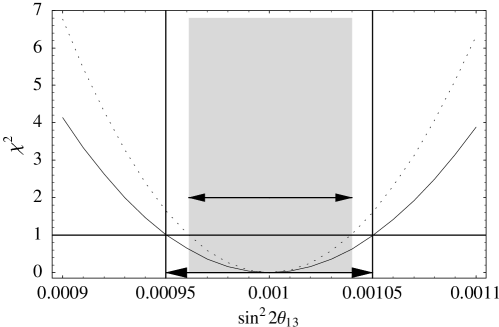
Quite frequently an analysis is based on small or moderate event rates in the binned energy spectrum with fluctuations in each bin following a statistical distribution. This requires a careful statistical treatment, which is described in Appendix C. In the end, a certain measurement can always be fit to the theoretical prediction with a suitably defined confidence level. For a given confidence level and one parameter considered, an interval of allowed values can be determined. The absolute width of this interval is the statistical error, which can be quite large even if we do not take other error sources into account. Our method can thus deal appropriately with small event rates and also converges to Gaussian statistics for large event rates. As an example, the $\chi^{2}$–function is plotted in Figure 1 as function of $\sin^{2}2\theta_{13}$. The figure illustrates that all values of $\sin^{2}2\theta_{13}$ for which the $\chi^{2}$–function is below the value corresponding to the chosen confidence level fit the true value $\sin^{2}2\theta_{13}=0.001$.

Figure 1: The $\chi^{2}$–function of the statistical error plotted as function of $\sin^{2}2\theta_{13}$ for the true value $\sin^{2}2\theta_{13}=0.001$. The arrows indicate the error in $\sin^{2}2\theta_{13}$ read off on the $1\sigma$ confidence level. In this example, we choose the NuFact-II scenario with the LMA solution in Equation (5) but $\Delta m_{21}^{2}=4.5\cdot 10^{-5}\,\mathrm{eV}$ and $\sin^{2}2\theta_{12}=1.0$.

3.2 Systematical errors

We consider a number of systematical limitations, such as errors in overall signal and background normalizations, energy dependent normalizations (tilts), efficiencies, cross sections, the energy threshold functions. Whenever relevant, we will analyze these errors separately and talk about “systematics” in the context of errors in signal and background normalizations and tilts, which also includes the uncertainties in the efficiencies. As usual, the considered systematical errors make the confidence intervals obtained from the statistical errors somewhat larger, but not by an order of magnitude. The typical effect of switching on systematical errors is illustrated in Figure 2.

Figure 2: The $\chi^{2}$–function of the statistical (dotted curve) and statistical plus systematical (solid curve) error as function of $\sin^{2}2\theta_{13}$ for the true value $\sin^{2}2\theta_{13}=0.001$. The vertical lines indicate the new overall error in $\sin^{2}2\theta_{13}$ read off on the $1\sigma$ confidence level, being somewhat larger than the statistical error illustrated by the shaded region. In this example, we choose the NuFact-II scenario with the LMA solution in Equation (5) but $\Delta m_{21}^{2}=4.5\cdot 10^{-5}\,\mathrm{eV}$ and $\sin^{2}2\theta_{12}=1.0$.

3.3 Correlation errors

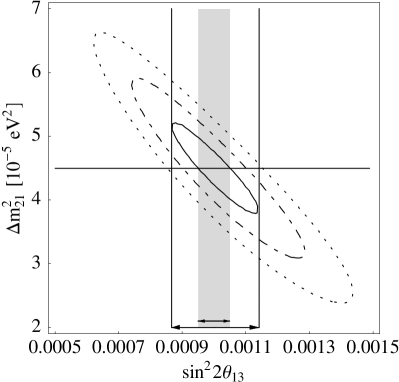
The underlying oscillation framework is based on trigonometric expressions where two or more parameters can be correlated in the sense that an experiment is dominantly sensitive to a certain parameter combination. Weaker information on other parameter combinations allows typically to disentangle the parameters, but some correlations survive. This is nothing but the simple fact that measuring a sum $a+b$ does not determine the individual values of $a$ and $b$. Weaker information on other combinations of $a$ and $b$ produces then egg–shaped regions aligned along $a+b=const.$. Insisting on a measurement of $a$ leads then, without better knowledge on $b$, to a projection onto the $a$-axis, which gives a sizable error in $a$. If the value of $b$ were, however, fixed artificially to some number, the error in $a$ would artificially appear to be much smaller and would not represent the proper measurement error of the experiment. In addition, its central value would depend on the chosen value of $b$. This simple two–parameter correlation example should illustrate, that two– and even multi–parameter correlations make long baseline studies more complicated. Figure 3 illustrates this problem for a realistic two–parameter correlation between $\sin^{2}2\theta_{13}$ and $\Delta m_{21}^{2}$.

Figure 3: The $1\sigma$ (solid curve), $2\sigma$ (dashed curve), and $3\sigma$ (dotted curve) contours of the $\chi^{2}$–function including statistical and systematical errors, which is plotted as function of $\sin^{2}2\theta_{13}$ and $\Delta m_{21}^{2}$ for the true values $\sin^{2}2\theta_{13}=0.001$ and $\Delta m_{21}^{2}=4.5\cdot 10^{-5}\,\mathrm{eV}^{2}$. The vertical lines indicate the new overall error in $\sin^{2}2\theta_{13}$, coming from the correlation with $\Delta m_{21}^{2}$ and read off on the $1\sigma$ confidence level. It is considerably larger than the systematical plus statistical error marked by the shaded region obtained for the fixed value $\Delta m_{21}^{2}=4.5\cdot 10^{-5}\,\mathrm{eV}^{2}$, indicated by the horizontal line. In this example, we choose the NuFact-II scenario with the standard LMA solution in Equation (5) but $\sin^{2}2\theta_{12}=1.0$.

3.4 External input

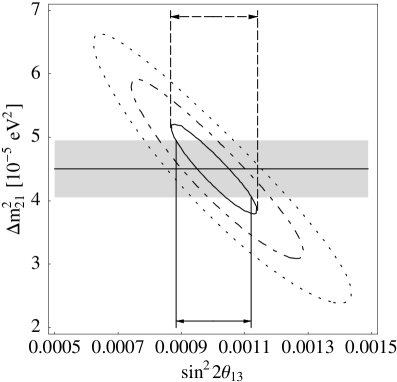
External information on the measured observables can and should be added to the analysis to constrain the allowed regions in the parameter space as good as possible. The atmospheric oscillation parameter measurements are with the discussed setups much preciser than the pre–existing information, even compared to the MINOS or ICARUS experiments [39] – assuming that the old and new measurements are consistent, of course. For those parameters, external input can therefore be ignored. This is different for the measurements of the solar mass squared difference and mixing angle, which are done by the KamLAND experiment. Similarly, the Earth’s matter density profile, as given in the PREM model (Preliminary Reference Earth Model), should be included as an essential external input. One might take the attitude that external input could be added later by some global fit. However, it can help to resolve or reduce correlations in a way which is not possible afterwards. In some cases, external input even can change the measurement errors by many orders of magnitude, which again can not be included properly afterwards. Figure 4 demonstrates how the error in $\sin^{2}2\theta_{13}$ coming from statistics, systematics, and correlations, is reduced by using external information on $\Delta m_{21}^{2}$.

Figure 4: The $1\sigma$ (solid curve), $2\sigma$ (dashed curve), and $3\sigma$ (dotted curve) contours of the $\chi^{2}$–function including statistical, systematical, and correlational errors, which is plotted as function of $\sin^{2}2\theta_{13}$ and $\Delta m_{21}^{2}$ for the true values $\sin^{2}2\theta_{13}=0.001$ and $\Delta m_{21}^{2}=4.5\cdot 10^{-5}\,\mathrm{eV}^{2}$. The arrows on the bottom indicate the new overall error in $\sin^{2}2\theta_{13}$ including the external input, which is in this case a $10\%$ precision measurement of $\Delta m_{21}^{2}$ marked by the shaded region. This external measurement favors possible values of $\sin^{2}2\theta_{13}$ in the shaded region, which makes the error in $\sin^{2}2\theta_{13}$ without external information, indicated by the dashed arrow on the top, shrink. In this example, we again choose the NuFact-II scenario with the LMA solution in Equation (5) but $\sin^{2}2\theta_{12}=1.0$.

3.5 Degeneracy errors

Degeneracies occur if two or more separated parameter sets fit the same data. This sort of error is important because it can quite substantially affect the error of a measurement, but it is completely different from the ones discussed above. Dealing with degeneracies, one might, for example, either quote separate errors for completely separated parameter sets, or take the whole range covered by the degeneracies as the measurement error. Degeneracies will be discussed in somewhat greater detail in Section 5.

4 The oscillation framework

We assume standard three neutrino mixing. The leptonic mixing matrix $U$ is parameterized in the same way as the quark mixing matrix [28]. The probabilities for the neutrino transitions $\nu_{\alpha}\rightarrow\nu_{\beta}$ in vacuum are for $n$ neutrino flavors given by

$$P_{\alpha\beta}=\delta_{\alpha\beta}-4\;\underset{i>j}{\sum\limits_{i=1}^{n}\sum\limits_{j=1}^{n}}\operatorname{Re}J_{ij}^{\alpha\beta}\sin^{2}\Delta_{ij}-2\;\underset{i>j}{\sum\limits_{i=1}^{n}\sum\limits_{j=1}^{n}}\operatorname{Im}J_{ij}^{\alpha\beta}\sin 2\Delta_{ij}~{},$$ (1)

where $J_{ij}^{\alpha\beta}\equiv U_{\alpha i}U^{*}_{\alpha j}U^{*}_{\beta i}U_{\beta j}$ and $\Delta_{ij}\equiv\Delta m^{2}_{ij}L/(4E_{\nu})\equiv(m_{i}^{2}-m_{j}^{2})L/(4E_{\nu})$. Moreover, we define $\Delta\equiv\Delta_{31}$. We will present results based on a full numerical simulation including matter effects. It is, however, very useful to have at least a qualitative, analytical understanding of the effects. The oscillation probabilities are, in principle, exactly known, but the full expressions are quite lengthy and do not allow much insight. We therefore use simplified expressions by expanding the probabilities in Equation (1) simultaneously in the small mass hierarchy parameter $\alpha\equiv{\Delta m^{2}_{21}}/{\Delta m^{2}_{31}}$ and the small mixing angle $\sin 2\theta_{13}$. The terms can be ordered by their combined power of small quantities as well as matter effects can be included [9, 33, 4]. The expansion in $\sin 2\theta_{13}$ is always good, since this mixing angle is known to be small. The expansion in $\alpha$ is a good approximation as long as the oscillation governed by the solar mass squared difference is small compared to the leading atmospheric oscillation, i.e., $\alpha\,\Delta\lesssim 1$. The expansion in $\alpha$ can therefore be used for baselines below

$$L\lesssim 8000\,\mathrm{km}\left(\frac{E_{\nu}}{\,\mathrm{GeV}}\right)\left(\frac{10^{-4}\,\mathrm{eV}^{2}}{{\Delta m^{2}_{21}}}\right),$$ (2)

which is fulfilled for the studied experiments. The leading terms in small quantities are for the vacuum appearance probabilities and disappearance probabilities

$$P_{e\mu} \simeq \sin^{2}2\theta_{13}\,\sin^{2}\theta_{23}\sin^{2}{\Delta}$$ (3)

$$\mp \alpha\;\sin 2\theta_{13}\,\sin\delta_{\mathrm{CP}}\,\cos\theta_{13}\sin 2\theta_{12}\sin 2\theta_{23}\sin^{3}{\Delta}$$

$$- \alpha\;\sin 2\theta_{13}\,\cos\delta_{\mathrm{CP}}\,\cos\theta_{13}\sin 2\theta_{12}\sin 2\theta_{23}\cos{\Delta}\sin^{2}{\Delta}$$

$$+ \alpha^{2}\,\cos^{2}\theta_{23}\sin^{2}2\theta_{12}\sin^{2}{\Delta},$$

$$P_{\mu\mu} \simeq 1-\cos^{2}\theta_{13}\sin^{2}2\theta_{23}\sin^{2}{\Delta}$$ (4)

$$+ 2\alpha\cos^{2}\theta_{13}\cos^{2}\theta_{12}\sin^{2}2\theta_{23}{\Delta}\cos{\Delta}.$$

The next terms in this expansion can be ignored for a qualitative discussion, since they are suppressed by an extra power of one of the small parameters $\alpha$ and $\sin 2\theta_{13}$. The actual numerical values of $\alpha$ and $\sin^{2}2\theta_{13}$ give each term in Equations (4) and (3) a relative weight. In the LMA case, we have $\alpha\simeq 10^{-2\pm 1}$. This means that the first term in Equation (3) is dominating for $\sin^{2}2\theta_{13}\simeq 0.1$ close to the CHOOZ bound, which, for example, can make it harder to extract the CP violating information contained in the $\alpha\cdot\sin 2\theta_{13}$ terms. For smaller values of $\sin 2\theta_{13}\simeq\alpha$ all terms contribute equally. The $\alpha^{2}$ term finally dominates for tiny $\sin 2\theta_{13}\ll\alpha$, where it again becomes difficult to extract the CP-parameters from the $\alpha\cdot\sin 2\theta_{13}$ terms in Equation (3). One can in general observe in Equations (3) and (4) that the CP phase can be measured in the appearance channel if $\alpha$ is not too small, i.e., in the LMA case. Note, however, that $\alpha$ should also not be too large compared to $\sin 2\theta_{13}$, since in this case the $\alpha^{2}$ terms start to dominate, which reduces the relative size of the CP violating effects and leads to a reduced CP sensitivity even though the event rates are growing. For neutrino factories, this has been demonstrated in detail in Ref. [9, 33]. Note that our analysis takes into account the complete dependence on the CP phase, involving the CP odd $\sin\delta_{\mathrm{CP}}$–term and the CP even $\cos\delta_{\mathrm{CP}}$–term.

The smallness of $\alpha$ and $\theta_{13}$ justifies the categorization of the parameters into leading, subleading, and subsubleading parameters [9]. For $\alpha\rightarrow 0$ (which is equivalent to $\Delta m_{21}^{2}\rightarrow 0$) and $\theta_{13}\rightarrow 0$, the appearance channel is suppressed, leading to the two–flavor neutrino oscillations in the disappearance channel, governed by $\theta_{23}$ and $\Delta m_{31}^{2}$. We call these parameters leading parameters, which are already measured by atmospheric neutrino experiments [40, 41, 42]. Future long baseline experiments will allow high precision measurements of these parameters. For $\Delta m_{21}^{2}\rightarrow 0$ and $\theta_{13}\neq 0$ the first term in the appearance probability in Equation (3) becomes non-zero. Since the sign of $\Delta m_{31}$ also enters this term after the inclusion of matter effects [3, 6, 43], we call $\theta_{13}$ and the sign of $\Delta m_{31}$ subleading parameters. They could even be measured very precisely without the LMA solution. Finally, for $\Delta m_{21}^{2}\neq 0$ and $\theta_{13}\neq 0$, the remaining terms in Equations (3) and (4) are switched on. These contain the additional parameters $\Delta m_{21}^{2}$, $\theta_{12}$, and $\delta_{\mathrm{CP}}$, which we call the subsubleading parameters. Note that every term in Equation (3) only depends on the product $\Delta m_{21}^{2}\sin 2\theta_{12}$. Other experiments (or oscillation channels) are thus required to measure the individual parameters and we will see that external input, such as on $\Delta m_{21}^{2}$ from the KamLAND experiment, is essential to improve the precision on $\sin^{2}2\theta_{13}$ and $\delta_{\mathrm{CP}}$.

The above formalism will be used in this paper to understand the effects analytically. The shown results are, however, based on event rates calculated from the full oscillation formulas, including sizable corrections due to matter effects [44, 45, 46, 47]. Analytical expressions for the transition probabilities in matter can be found in Refs. [3, 33, 4].

5 Degeneracies

The trigonometric neutrino oscillation probabilities have, as already mentioned in Section 3, degenerate solutions, which require an approach different from the one to the statistical, systematical, correlational, and external errors discussed in Section 3. Degeneracies allow additional solutions, which may lie close to the best–fit solution or at completely different positions in the parameter space. Well–separated degenerate solutions do not affect the shape of the original fit manifold around a best–fit point and do not change the size of the measurement error as we have defined it so far. Degeneracies can in principle be resolved by improving the experimental performance such by using more than one baseline or better energy resolution. Degeneracies will be important for this work, since we compare setups which can not resolve the degeneracies. We will comment on the combination of experiments in the discussion in Section 8.

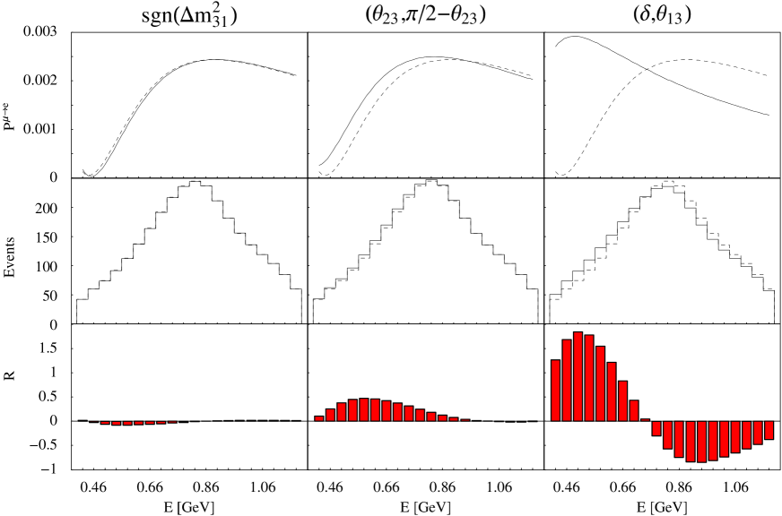
There are three independent two–fold degeneracies, i.e., an overall “eight–fold” degeneracy, which has been discussed analytically in terms of transition probabilities in Ref. [48]. We study the consequences of these degeneracies in our event rate based analysis, where we focus mostly on the measurements of $\sin^{2}2\theta_{13}$ and $\delta_{\mathrm{CP}}$. The three potential degeneracies can already be seen in Equations (3) and (4) and are summarized as follows:

Figure 5: For JHF-HK: The transition probabilities (first row), the binned event rates (second row), and the ratios $R\equiv(N_{i}-N_{i}^{0})/\sqrt{(N_{i}+N_{i}^{0})/2}$ (third row) for the charged current neutrino events in the appearance channel. The columns represent the possible degenerate solutions referred to by the labels on the top. The solid curves show the degenerate solutions and the dashed curves the the best–fit solutions. The quantity $R$ gives an idea of the statistical weighting of the individual event rates $N_{i}$ in the bins $i$ compared to the best–fit rates $N_{i}^{0}$ (figure of merit). For the parameters, we choose the LMA solution but $\Delta m_{21}^{2}=4.5\cdot 10^{-5}\,\mathrm{eV}$, $\sin^{2}2\theta_{12}=1.0$, $\sin^{2}2\theta_{13}=0.01$, $\delta_{\mathrm{CP}}=\pi/4$, and $\theta_{23}=\pi/4-0.2$ in order to be able to observe all degeneracies.

Figure 6: For NuFact-II: The transition probabilities (first row), the binned event rates (second row), and the ratios $R\equiv(N_{i}-N_{i}^{0})/\sqrt{(N_{i}+N_{i}^{0})/2}$ (third row) for the charged current neutrino events in the appearance channel. The columns represent the possible degenerate solutions referred to by the labels on the top. The solid curves show the degenerate solutions and the dashed curves the the best–fit solutions. The quantity $R$ gives an idea of the statistical weighting of the individual event rates $N_{i}$ in the bins $i$ compared to the best–fit rates $N_{i}^{0}$ (figure of merit). For the parameters, we choose the LMA solution but $\Delta m_{21}^{2}=4.5\cdot 10^{-5}\,\mathrm{eV}$, $\sin^{2}2\theta_{12}=1.0$, $\sin^{2}2\theta_{13}=0.01$, $\delta_{\mathrm{CP}}=\pi/4$, and $\theta_{23}=\pi/4-0.2$ in order to be able to observe all degeneracies.

Figure 7: The $3\sigma$ contours of the $\chi^{2}$–function, which is plotted as function of $\delta_{\mathrm{CP}}$ and $\sin^{2}2\theta_{13}$ for the JHF-HK (left–hand plot) and NuFact-II (right–hand plot) experiments. The solid curves refer to the original solution at the best–fit point, the dashed curves to the degeneracy in $(\theta_{23},\pi/2-\theta_{23})$, and the the dotted curve to the degeneracy in $\mathrm{sgn}(\Delta m_{31}^{2})$. The diamonds mark the local minima with the respective $\chi^{2}$–values. The arrows on the left–hand sides of the plots illustrate the measurement error in $\sin^{2}2\theta_{13}$ from statistical, systematical, external, and correlational sources, as we had it at the end of Section 3. The arrows on the right–hand sides of the plots mark the overall error, as we would have it for taking the whole range covered by degeneracies, given by the gray–shaded region. For the oscillation parameters, we choose the LMA solution with $\Delta m_{21}^{2}=4.5\cdot 10^{-5}\,\mathrm{eV}$, $\sin^{2}2\theta_{12}=1.0$, $\sin^{2}2\theta_{13}=0.01$, $\delta_{\mathrm{CP}}=\pi/4$, and $\sin^{2}2\theta_{23}=\pi/4-0.2$.

Figure 8: The position $\delta^{\prime}$ of the degenerate solution (in $\mathrm{sgn}(\Delta m_{31}^{2})$) plotted as function of the true value of $\sin^{2}2\theta_{13}$, lying approximately at $(\sin^{2}2\theta_{13})^{\prime}\simeq\sin^{2}2\theta_{13}$ of the best–fit solution. The plots show the JHF-HK (left–hand plot) and NuFact-II (right–hand plot) experiments for the true values $\delta_{0}=+1/2\pi$ (black curve) and $\delta_{0}=-1/2\pi$ (gray curve). The dashed sections of the curves indicate the values of $\sin^{2}2\theta_{13}$ where the degenerate solution can not be observed on the $2\sigma$ confidence level, whereas it can be observed in the solid sections. For the oscillation parameters, we choose the LMA solution.

The sign of $\Delta m_{31}^{2}$:

Vacuum oscillations do not depend on the sign of $\Delta\equiv\Delta m^{2}_{31}L/4E_{\nu}$. This degeneracy can, in principle, be lifted by MSW effects in matter. A degenerate solution for the opposite sign of $\Delta m_{31}^{2}$ may survive, however, for a different value of $\delta_{\mathrm{CP}}$ and almost the same value of $\sin^{2}2\theta_{13}$ [16].

Non–maximal mixing $(\theta_{23},\pi/2-\theta_{23})$:

For $\theta_{23}\neq\pi/4$, a degenerate solution exists at approximately $\theta^{\prime}_{23}=\pi/2-\theta_{23}$. For our setups, it turns out to be at a similar value of $\delta_{\mathrm{CP}}$. This degeneracy can also be seen in Equations (3) and (4), where the factor of $\sin^{2}\theta_{23}$ in the first term of Equation (3) and the factor of $\cos^{2}\theta_{23}$ in the fourth term of Equation (3) are exchanged under the transformation $\theta_{23}\rightarrow\pi/2-\theta_{23}$, leading to a possible compensation by changing $\sin^{2}2\theta_{13}$.

The $(\delta,\theta_{13})$ ambiguity:

Equation (3) allows that in many cases a combination of $(\delta,\theta_{13})$ gives the same probabilities as another pair $(\delta^{\prime},\theta_{13}^{\prime})$ [8]. Taking into account the appearance channel only and ignoring matter effects, the asymmetry of the $\sin\delta_{\mathrm{CP}}$ term under a neutrino–antineutrino transformation opens the possibility of a CP violation measurement. From this point of view, this degeneracy can be seen in the total event rates as neutrino and anti neutrino rates equal to the best–fit point. However, the energy resolution of the experiment allows, in principle, to resolve the degeneracy (for the dependence on experimental details, see Refs. [8, 9] and Appendix B).

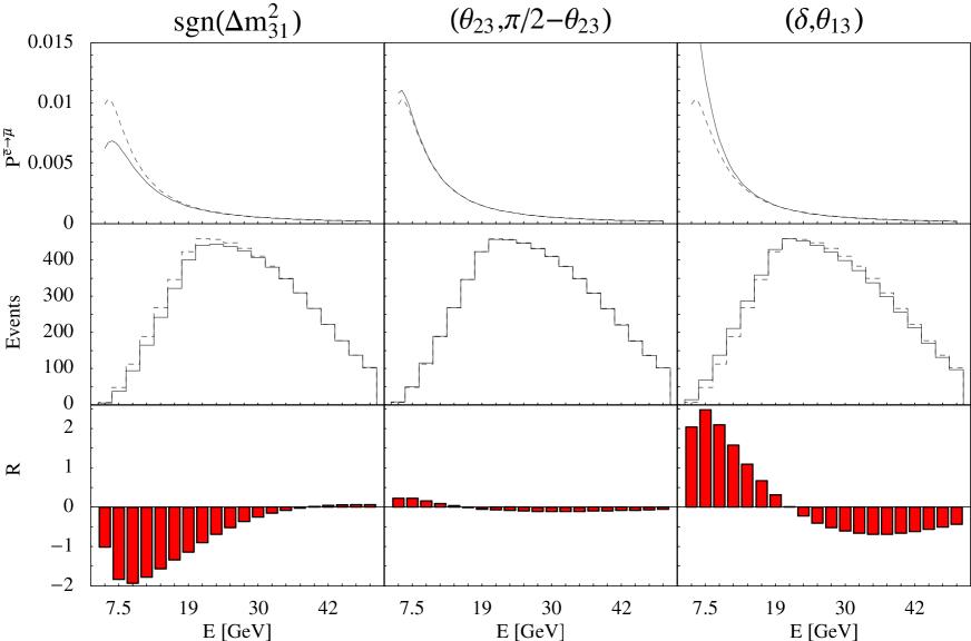
We illustrate the above ambiguities for our experimental setups for a parameter set, for which all effects can be seen, i.e., if not otherwise stated, we choose $\delta_{\mathrm{CP}}=\pi/4$, $\sin^{2}2\theta_{13}=0.01$, and $\sin^{2}2\theta_{23}=\pi/4-0.2$. Figures 5 (for JHF-HK) and 6 (for NuFact-II) show for the $\nu_{e}\rightarrow\nu_{\mu}$ appearance channel the transition probabilities (first row), the binned event rates (second row), and the the ratios $R\equiv(N_{i}-N_{i}^{0})/\sqrt{(N_{i}+N_{i}^{0})/2}$ (third row). Every column corresponds to one type of degeneracy. The dashed and solid curves correspond for the upper two rows to the best–fit and the degenerate solution, respectively. The ratio $R$ gives an idea of the statistical weight of the individual event rates $N_{i}$ in the bins $i$ compared to the rates $N_{i}^{0}$ of the best–fit solution (figure of merit). For the JHF-HK experiment in Figure 5, the degeneracies in $\mathrm{sgn}(\Delta m_{31}^{2})$ and $(\theta_{23},\pi/2-\theta_{23})$ lead only to small statistical deviations from the best–fit spectra and can, in principle, be observed for our setups. It is interesting how the very different transition probabilities in the $(\delta,\theta_{13})$ case lead to similar event rate spectra and identical total rates. From the $R$ distribution it becomes clear that this degeneracy can be resolved if the experiment has sufficient energy resolution. For our experimental setups, it turns out that this degeneracy is hardly be observed for large $\sin^{2}2\theta_{13}$, while it is quite important at the sensitivity limit. The neutrino factory is for comparison shown in Figure 6. The degenerate event rate spectra seem to be very similar, but the overall event rates are considerably larger and statistics is thus very good. The $R$ distributions show why only the $(\theta_{23},\pi/2-\theta_{23})$ degeneracy survives in a fit of the event rate spectrum. Compared to the JHF-HK experiment, the degeneracy in $\mathrm{sgn}(\Delta m_{31}^{2})$ can be resolved at the used value of $\sin^{2}2\theta_{13}$ due to MSW matter effects at this long baseline. The point is that the matter density resonance energy in Earth (of about $15\,\mathrm{GeV}$) lies within the energy window of the detector and its effects can clearly be seen in the $R$ distribution. We will see in Figure 8, that this degeneracy can not be resolved anymore for very small values of $\sin^{2}2\theta_{13}$, since the reduced event rates (overall and per bin) do not allow to use the spectral information to resolve this degeneracy, even though $\sin^{2}2\theta_{13}$ can still be extracted from the total rates. Matter effects play a minor role for the $(\delta,\theta_{13})$ degeneracy and the similar qualitative behavior of both experiments is determined by the the fact that both are operated at a similar value of $L/E$. The $(\delta,\theta_{13})$ ambiguity therefore looks very similar for the NuFact-II and the JHF-HK setup, as can be seen from the $R$ distributions.

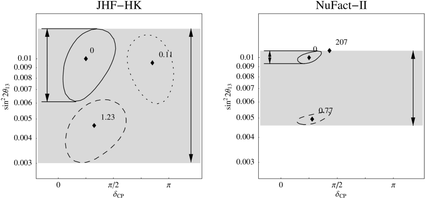
Figure 7 shows fits of $\sin^{2}2\theta_{13}$ versus $\delta_{\mathrm{CP}}$ for the JHF-HK and NuFact-II experiments at the $3\sigma$ confidence level, where the respective $\chi^{2}$ values at the local minima are specified. Besides the best–fit there exist also degenerate solutions in $\mathrm{sgn}(\Delta m_{31}^{2})$ and $(\theta_{23},\pi/2-\theta_{23})$. The figure illustrates that, for the chosen parameter values, all of the shown degeneracies can be observed at the $3\sigma$ confidence level except from the degeneracy in $\mathrm{sgn}(\Delta m_{31}^{2})$ for the neutrino factory. The figures also show the pattern which was mentioned before: The $\mathrm{sgn}(\Delta m_{31}^{2})$ degeneracy lies more or less at the same value of $\sin^{2}2\theta_{13}$, but at a different value of $\delta_{\mathrm{CP}}$. The $(\theta_{23},\pi/2-\theta_{23})$ degeneracy lies at a similar value of $\delta_{\mathrm{CP}}$ and a different value of $\sin^{2}2\theta_{13}$. The $\mathrm{sgn}(\Delta m_{31}^{2})$ degeneracy will thus especially affect the CP measurement, while the $(\theta_{23},\pi/2-\theta_{23})$ degeneracy will especially affect the $\sin^{2}2\theta_{13}$ measurement. We will return to this issue at the end of this section, in order to explain how the degeneracies are included in our evaluations.

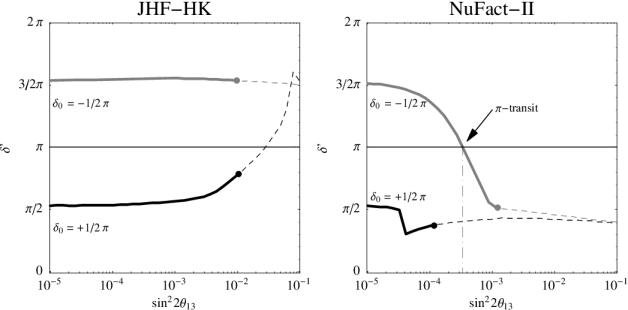
We mentioned before and illustrated in Figure 8 that the presence of the $\mathrm{sgn}(\Delta m_{31}^{2})$ degeneracy depends on the value of $\sin^{2}2\theta_{13}$. Figure 8 shows, as a function of $\sin^{2}2\theta_{13}\simeq\sin^{2}2\theta_{13}^{\prime}$, the position of the degenerate solution $\delta^{\prime}$ resulting from the $\mathrm{sgn}(\Delta m_{31}^{2})$ degeneracy. The black curves correspond to true values $\delta_{0}=\pi/2$ and the gray curves to $\delta_{0}=3\pi/2$, which means that the best–fit solutions would be represented by the horizontal lines $\delta_{\mathrm{CP}}\equiv\pi/2$ and $\delta_{\mathrm{CP}}\equiv 3\pi/2$, respectively, independently of $\sin^{2}2\theta_{13}$. The dashed extrapolated curves indicate the regions where the degeneracy is resolved, i.e.where the degenerate solution is rejected at the $2\sigma$ confidence level. One can read off from Figure 8 that for $\sin^{2}2\theta_{13}=0.01$ this degeneracy does not show up at this confidence level for the NuFact-II experiment, but for the JHF-HK experiment. This corresponds to Figure 7, where $\sin^{2}2\theta_{13}=0.01$ was used. The degeneracies are in general resolved at large $\sin^{2}2\theta_{13}$ and they are cut off at small values of $\sin^{2}2\theta_{13}$ by the sensitivity limit, which is not shown in Figure 8. It is interesting to note that the degenerate solution tends to move away from the best–fit solution for large values of $\sin^{2}2\theta_{13}$, but approaches it for small values of $\sin^{2}2\theta_{13}$. Especially, it turns out that all starting values $\delta_{0}$ lead to solutions attracted by $\pi$/2 (NuFact-II) or $3\pi/2$ (JHF-HK) for large values of $\sin^{2}2\theta_{13}$, which implies that the degenerate solution moves most for the starting values $3\pi/2$ (NuFact-II) or $\pi/2$ (JHF-HK). Altogether, there are three important consequences for the $\sin^{2}2\theta_{13}$ dependence of CP studies, where the degeneracy in $\mathrm{sgn}(\Delta m_{31}^{2})$ is very important:

• The results will not be affected for large values of $\sin^{2}2\theta_{13}$ since the degeneracy can be resolved.

• If there is sensitivity for $\sin^{2}2\theta_{13}$ smaller than about $10^{-4}$ (NuFact-II) or $10^{-3}$ (JHF-HK), then the degenerate solution joins with the best–fit point and thus becomes irrelevant.

• Especially for a neutrino factory with $\sin^{2}2\theta_{13}$ between about $10^{-3}$ and $10^{-4}$, the degeneracy can move $\delta$ very far away from its true value especially for $\delta_{0}=3\pi/2$, which implies a complex structure in corresponding plots. The degenerate solution crosses, for example, the line $\delta^{\prime}=\pi$ at about $\sin^{2}2\theta_{13}=3\cdot 10^{-4}$ (labeled “$\pi$–transit” in Figure 8), which means that CP violation could not be distinguished from CP conservation at this transit point (cf., Figures 17 and 18 in the next section).

Coming back to Figure 7, we still need to discuss how to treat degeneracy errors, i.e., how we obtain a total error including the degeneracies. One could, for example, simply take the measurement error of $\sin^{2}2\theta_{13}$ at the best–fit point purely from statistical, systematical, external, and correlational errors. This optimistic choice is illustrated by the arrows on the left–hand sides of the plots and simply ignores the existence of degenerate solutions. However, it is obvious that without additional external input the degeneracies can not be resolved. An alternative would be to take the worst case errors marked by the arrows on the right–hand sides of the plots, which is identical to the gray–shaded region covering the range of all possible degeneracies (pessimistic choice). A look at the two plots shown in Figure 7 tells us that one must take the complexity of the problem into account. The shown JHF-HK case is obviously better described by the pessimistic case, since the degenerate solutions are almost touching each other. For the NuFact-II case it would, however, make more sense to quote the two separated (degenerate) fit regions with their individual errors. However, the pessimistic choice would obviously lead to a very different precision, which can be an order of magnitude worse. It should be obvious that one must look at the specific case at hand to decide which point of view is more appropriate. In most cases we will therefore show figures with and without degenerate solutions and we will discuss the degeneracy problem wherever appropriate.

6 Results I: The measurement of $\sin^{2}2\theta_{13}$

We now present our results concerning the experimental capabilities to measure $\sin^{2}2\theta_{13}$. This includes an analysis of the impact factors on the measurement, a discussion of the $\sin^{2}2\theta_{13}$ sensitivity, and an evaluation of the precision of the $\sin^{2}2\theta_{13}$ measurement. We also investigate the sensitivity to the sign of $\Delta m_{31}^{2}$, which is a closely related issue.

All results of of this and the following section are, unless otherwise stated, calculated for the current best–fit values of the atmospheric [49, 50] and solar neutrino experiments [51, 52]. The ranges are given at the $3\sigma$ confidence level by

$${\Delta m^{2}_{31}} = 3_{-2}^{+5}\cdot 10^{-3}\,\mathrm{eV}^{2},$$

$$\sin^{2}2\theta_{23} = 1_{-0.2}^{+0},$$

$${\Delta m^{2}_{21}} = 3.7_{-2}^{+42}\cdot 10^{-5}\,\mathrm{eV}^{2},$$

$$\sin^{2}2\theta_{12} = 0.8_{-0.2}^{+0.2},$$

$${\Delta m^{2}_{21}}\sin^{2}2\theta_{12} = 3_{-1.8}^{+38}\cdot 10^{-5}\,\mathrm{eV}^{2},$$ (5)

where the mean values are throughout the text referred to as the “LMA solution”. The indicated ranges represent the current knowledge to be kept in mind for our analysis. For $\sin^{2}2\theta_{13}$ we will only allow values below the CHOOZ bound [53] and the used value will be specified in the respective examples. For the CP phase $\delta_{\mathrm{CP}}$, we choose $\delta_{\mathrm{CP}}=0$ as standard value if not otherwise stated. In some cases we use, however, parameters different from Equation (5), to demonstrate specific effects. An example are degenerate solutions in $(\theta_{23},\pi/2-\theta_{23})$, which are only observable for $\sin^{2}2\theta_{23}<1$.

6.1 Impact factors on the measurement of $\sin^{2}2\theta_{13}$

In order to identify the relevant and controllable main contributions to the errors of the measurement of $\sin^{2}2\theta_{13}$, we define the impact factor $\mathrm{IF}_{\xi}$ of an error source $\xi$ as

$$\mathrm{IF}_{\xi}\equiv 1-\frac{(\delta\sin^{2}2\theta_{13})_{\mathrm{Error\,source\,\xi\,off}}}{(\delta\sin^{2}2\theta_{13})_{\mathrm{All\,error\,sources\,on}}},$$ (6)

where $\delta\sin^{2}2\theta_{13}$ is the total error of the measurement of $\sin^{2}2\theta_{13}$ chosen at the $2\sigma$ confidence level, including the statistical, systematical, correlational, and external errors (cf., Figure 4). The impact factor specifies the relative impact of a certain source of errors $\xi$ on the total error of the measurement, i.e., the error source $\xi$ is switched off compared to taking into account all error sources. In this section, we especially focus on the relative contributions of systematical and correlational errors in order to determine the main sources limiting the precision of the studied experiments. For the moment, we do not take into account degeneracies and focus on the best–fit solution, since we are interested in how the size of the individual solutions is reduced (e.g., as shown in Figure 7). Figure 9 shows for the four different setups the relative contributions of the impact factors for three different values of $\sin^{2}2\theta_{13}$. As error sources $\xi$ we include systematical errors, the correlations with the mass squared differences and $\theta_{23}$, the energy threshold function (for details, see Appendix B), and the uncertainty in the matter density (assumed to be $5\%$). Note that we include the external input from the KamLAND experiment for the solar parameters, which means that without this information the pie slices of the small mass squared difference could be larger.

Figure 9: The relative contributions of the impact factors on the measurement of $\sin^{2}2\theta_{13}$ for different experiments and different values of $\sin^{2}2\theta_{13}$. The error sources $\xi$ are the systematical errors (“Syst”), the correlations with the large (“$\Delta m_{31}^{2}$”) and small (“$\Delta m_{21}^{2}$”) mass squared differences, the correlation with the mixing angle $\theta_{23}$ (“$\theta_{23}$”), the energy threshold function for neutrino factories (“$E_{\min}$”), and the uncertainty in the matter density (“$\rho$”). For the oscillation parameters, we choose the LMA solution.

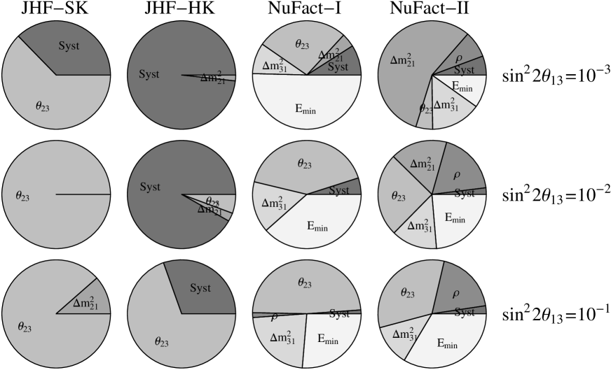
Before we analyze the behavior of the different setups in Figure 9 in detail, let us point towards the effects of the different values of $\sin^{2}2\theta_{13}$. In general, the smaller $\sin^{2}2\theta_{13}$ is, the smaller is the number of events we can expect to see in the appearance channels, which are dominating the precision of the $\sin^{2}2\theta_{13}$ measurement. This loss in statistics leads to a larger relative impact of the systematical errors.

JHF-SK

This setup leads only to a very low number of events and is thus statistics dominated. No single impact value contributes more than about 7 % to the absolute value. This comes essentially from the large statistical error in $\sin^{2}2\theta_{13}$ without any systematics and correlations, which means that the latter only modify the absolute error in a minor way. Note that for the JHF to Kamiokande experiments the baseline is too short for matter effects to play an important role.

JHF-HK

This setup leads to a very large number of events, i.e., very good statistics. Thus, especially for small values of $\sin^{2}2\theta_{13}$, the main impact comes from systematics. A closer analysis of the systematical impact factors shows that the systematical error is dominated by the background uncertainties of the charged current events. The remaining contributions are minor effects of the signal and background normalizations, as well as of the tilts. For this experiment, it is thus important to improve the understanding of background uncertainties, especially for the charged current events.

NuFact-I

The initial stage neutrino factory leads to a moderate number of events with a somewhat limited statistics dominating most effects. The main impact factors are the correlations with the leading oscillation parameters $\theta_{23}$ and $\Delta m_{31}^{2}$ as well as the energy threshold function. Especially for small values of $\sin^{2}2\theta_{13}$, the loss of low energy events due to the threshold function dominates. An extra detector component with a good coverage in the threshold energy regime or another improvement in the threshold properties would considerably help to improve the precision. Matter effect uncertainties are negligible at the achievable level of precision, even though the baseline is quite long in this setup.

NuFact-II

This setup has much better statistics than the initial stage neutrino factory. It is a high precision instrument for which the relative impact of all sources becomes quite important. Three points are especially interesting to observe: First, for small values of $\sin^{2}2\theta_{13}$, the correlation with the small mass squared difference dominates. The precision of this experiment depends therefore in this case on the precision of an external measurement, such as the KamLAND experiment. Better knowledge of $\Delta m_{21}^{2}$ than assumed would considerably help to improve the performance. Second, the energy threshold function dominates the errors for large $\sin^{2}2\theta_{13}$, probably because the low energy events have more relative weight. Again, a second detector with good coverage around the threshold energy or another improvement of the threshold properties would improve the precision. Third, because of the long baseline and the high precision, the matter density uncertainty is important, especially for large $\sin^{2}2\theta_{13}$ where the statistics is best.

In Figure 10, the impact factors are in addition shown for the sensitivity limit in $\sin^{2}2\theta_{13}$, since the behavior in $\sin^{2}2\theta_{13}$ can not necessarily extrapolated to this limit.

Figure 10: The relative contributions of the impact factors on the measurement of $\sin^{2}2\theta_{13}$ for different experiments at the sensitivity limit ($\sin^{2}2\theta_{13}=0$). The error sources $\xi$ are the systematical errors (“Syst”), the correlations with the large (“$\Delta m_{31}^{2}$”) and small (“$\Delta m_{21}^{2}$”) mass squared differences, the correlation with the mixing angle $\theta_{23}$ (“$\theta_{23}$”), the energy threshold function for neutrino factories (“$E_{\min}$”), and the uncertainty in the matter density (“$\rho$”). For the other oscillation parameters, we choose the LMA solution.

However, we do not observe a change in qualitative behavior from the plots in the first row of Figure 9 for all experiments except from the NuFact-II experiment. This part of the result is not very surprising, since for all experiments except from NuFact-II the sensitivity limit lies close to (or upper) $\sin^{2}2\theta_{13}=0.001$, which corresponds to the first row of Figure 9. The NuFact-II experiment, however, performs better and therefore the sensitivity limit is much lower. One can see from Figure 10 that in this case again the effect of the threshold function is the biggest impact factor.

Figure 11: The $\sin^{2}2\theta_{13}$ sensitivity on the $2\sigma$ confidence level for the different experiments on the right–hand side of the plot. Each bar represents the range of the sensitivity under a variation of the main impact factor (black bar) or a variation of the luminosity (gray bar), as labeled on the left–hand side of the respective bar. The left vertical dash on each bar corresponds to the optimistic choice, the middle vertical dash to our standard choice, and the right vertical dash to the pessimistic choice, where the meaning of each choice depends on the impact factor and is explained in the main text. For the oscillation parameters, we choose the LMA solution.

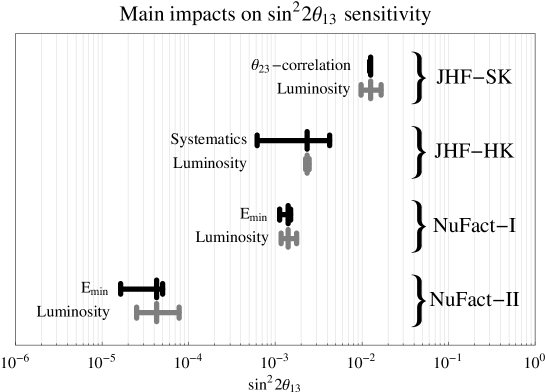
In order to summarize our results, we show in Figure 11 the $\sin^{2}2\theta_{13}$ sensitivity on the $2\sigma$ confidence level for all experiments. Each bar represents the range of the sensitivity under a variation of the main error impact or under a variation of the luminosity (number of stored muons times detector mass). The left dash on each bar corresponds to the optimistic choice, the middle dash to our standard choice, and the right dash to the pessimistic choice. For the luminosity, we choose twice the luminosity of our standard assumption as the optimistic choice and half the luminosity of our standard assumption as the pessimistic choice. For the main impact factors, we proceed similarly with the systematical uncertainties and double it or divide it by two. For the threshold function, represented by “$E_{\min}$”, we approximate it by a step function at $4\,\mathrm{GeV}$ (neutrino factory only) for the optimistic choice or replace it by a linear function climbing from $4$ to $25\,\mathrm{GeV}$ for the pessimistic choice instead of $4$ to $20\,\mathrm{GeV}$ for the standard choice. For the $\theta_{23}$–correlation, we eliminate it for the optimistic choice by assuming $\theta_{23}$ to be known from external input or keep it for the pessimistic choice, since $\theta_{23}$ is measured by the experiment itself. One can easily see that the JHF-SK experiment is statistics limited, i.e., changing the luminosity has the biggest impact. The JHF-HK experiment, however, is systematics limited. By improving the knowledge on the background uncertainties by a factor of two, the experiment would perform much better than by doubling the luminosity. The NuFact-I experiment would equally profit from higher statistics and a special low energy detector in order to lift the $(\delta,\theta_{13})$ ambiguity, which is for our setups especially important at the sensitivity limit. Similarly, a special low energy detector would help to improve the NuFact-II experiment, where the effect would be even better than doubling the luminosity.

6.2 The $\sin^{2}2\theta_{13}$ sensitivity

Here we analyze the $\sin^{2}2\theta_{13}$ sensitivity limit of our experimental setups, i.e., the minimum value of $\sin^{2}2\theta_{13}$ the experiments could distinguish from $\sin^{2}2\theta_{13}=0$ at the $90\%$ confidence level. Since we want to demonstrate the effects of the degenerate solutions, we show in Figure 12 two plots for different sets of parameters, where the $\sin^{2}2\theta_{13}$ sensitivity limit is plotted at 90% confidence level over the true values of $\sin^{2}2\theta_{13}$ and $\Delta m_{31}^{3}$ for the four different experiments (curves enveloping the shaded regions marking the regions of all superbeam– or neutrino factory–like experiments). The left–hand plot

Figure 12: The $\sin^{2}2\theta_{13}$ sensitivity limit at the 90% confidence level, plotted as function of the true values of $\sin^{2}2\theta_{13}$ and $\Delta m_{31}^{3}$ for the four different experiments. The shaded regions mark the regions of all superbeam–like (gray) or neutrino factory–like (black) experiments, where the left curve of each region is drawn for the initial stage experiment and the right curve for the advanced stage experiment. The left–hand plot is calculated for ${\Delta m^{2}_{21}}=0$ and $\sin^{2}2\theta_{23}=1.0$ and therefore degenerate solutions do not appear. The right–hand plot is drawn for ${\Delta m^{2}_{21}}=3\cdot 10^{-5}\,\mathrm{eV}^{2}$ and $\sin^{2}2\theta_{23}=0.8$ with all degeneracies taken into account (solid curves). The dashed curves in the right–hand plot correspond to not taking into account the $(\theta_{23},\pi/2-\theta_{23})$ degeneracy. For the other oscillation parameters, we choose the LMA solution.

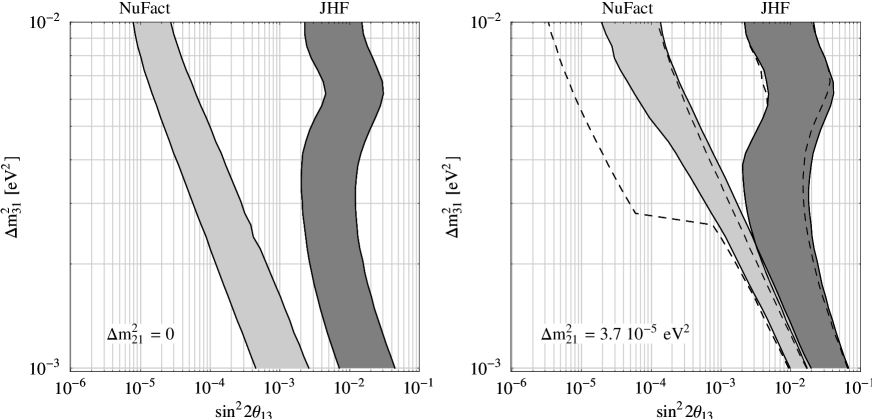
is produced for ${\Delta m^{2}_{21}}=0$ and $\sin^{2}2\theta_{23}=1.0$, implying that CP effects are switched off, and thus the $(\delta,\theta_{13})$ degeneracy, as well as the $(\theta_{23},\pi/2-\theta_{23})$ degeneracy because of $\sin^{2}2\theta_{23}=1.0$. The right–hand plot is calculated for ${\Delta m^{2}_{21}}=3\cdot 10^{-5}\,\mathrm{eV}^{2}$ and $\sin^{2}2\theta_{23}=0.8$ including these degeneracies by taking the worst case result over all degenerate solutions, since the experiments themselves can not resolve them. The dashed curves in this plot show the effect of the $(\theta_{23},\pi/2-\theta_{23})$ degeneracy being switched off, which means that the difference between the left–hand plot and the dashed curves in the right–hand plot essentially comes from $\Delta m_{21}^{2}$ effects, which are also controlling the $(\delta,\theta_{13})$ degeneracy. In Section 5 we have shown that this degeneracy is, because of the energy resolution, for large $\sin^{2}2\theta_{13}$ not present in the neutrino factory experiments. However, at the sensitivity limit there is quite poor statistics and almost no energy information, which means that the degenerate solution can not be resolved. As it is illustrated in Figure 7, the $\mathrm{sgn}(\Delta m_{31}^{2})$ degeneracy, lying at a similar value of $\sin^{2}2\theta_{13}$, does not influence the results very much. In summary, the JHF experiments are almost exclusively influenced by the $\Delta m_{21}^{2}$ effects and the $(\delta,\theta_{13})$ degeneracy, reducing the performance by an order of magnitude for small values of $\Delta m_{31}^{2}$. Though being systematics limited, they have less problems with degeneracies in general. The neutrino factory experiments, however, especially suffer for a large number of events from the degenerate solutions. For large $\Delta m_{31}^{2}$, the $(\theta_{23},\pi/2-\theta_{23})$ degeneracy dominates and for small $\Delta m_{31}^{2}$ the $(\delta,\theta_{13})$ degeneracy. It is important to note that the transition between both cases is close to the best–fit value of $\Delta m_{31}^{2}$, meaning that a somewhat smaller value of $\Delta m_{31}^{2}$ could also change our impact factor analysis in the last section slightly, since the $(\delta,\theta_{13})$ ambiguity is especially influenced by the threshold effects.

6.3 The $\sin^{2}2\theta_{13}$ precision

Compared to the $\sin^{2}2\theta_{13}$ sensitivity, the $\sin^{2}2\theta_{13}$ precision describes how precisely one can measure $\sin^{2}2\theta_{13}$, which depends on the true value of $\sin^{2}2\theta_{13}$, of course. Figure 13 shows the relative error on $\log\sin^{2}2\theta_{13}$ over the true value of $\sin^{2}2\theta_{13}$ for the four different experiments.

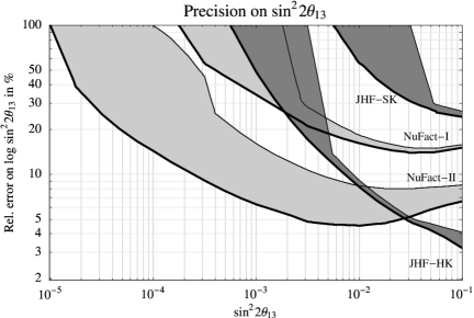
Figure 13: The relative error on $\log\sin^{2}2\theta_{13}$, plotted as function of the true value of $\sin^{2}2\theta_{13}$ for the four different experiments. The shaded regions indicate the error for all possible values of $\delta_{\mathrm{CP}}$, which means that the lower edge (thick curve) of each region corresponds to the best case and the upper edge (thin curve) to the worst case. For the oscillation parameters, we choose the LMA solution.

The shaded regions indicate the error for all possible values of $\delta_{\mathrm{CP}}$, which means that the lower edge of each region corresponds to the best case and the upper edge to the worst case. The lower (thick) curves would also correspond to the case of $\Delta m_{21}^{2}\rightarrow 0$ or $\alpha\rightarrow 0$ in Equation (3), which makes CP effects disappear. Especially, they would apply for the SMA, LOW, and VAC solutions. Degeneracies are not taken into account for this plot, i.e., we focus on the best–fit solution. This is quite a reasonable assumption, since $\sin^{2}2\theta_{23}=1$ (no $(\theta_{23},\pi/2-\theta_{23})$ degeneracy), $\sin^{2}2\theta_{13}$ is almost everywhere larger than the sensitivity limit (little effect of the $(\delta,\theta_{13})$ degeneracy), and the $\mathrm{sgn}(\Delta m_{31}^{2})$ degeneracy does not affect the $\sin^{2}2\theta_{13}$ measurement very much, as it is illustrated in Figure 7. All errors become very large at the respective sensitivity limits, because at the sensitivity limits the values of $\sin^{2}2\theta_{13}$ cannot be distinguished from zero anymore. As an important result, the NuFact-II experiment performs best except from large values of $\sin^{2}2\theta_{13}$, where the JHF-HK setup is better. As we have shown in Section 6.1, the neutrino factory measurement results are most strongly influenced by the matter density uncertainty for large $\sin^{2}2\theta_{13}$. One can show that the upward bending of the neutrino factory curves for large $\sin^{2}2\theta_{13}$ especially comes from the increasing importance of the matter density uncertainty.

6.4 The sign of $\Delta m_{31}^{2}$ sensitivity

In addition to the measurement of $\sin^{2}2\theta_{13}$, one can ask for the sensitivity to the sign of $\Delta m_{31}^{2}$, i.e., what the smallest value of $\sin^{2}2\theta_{13}$ is, for which the sign of $\Delta m_{31}^{2}$ could be measured. As we know from Section 5, there exists a degeneracy in the sign of $\Delta m_{31}^{2}$. Since the two possible cases ${\Delta m^{2}_{31}}<0$ and ${\Delta m^{2}_{31}}>0$ to be distinguished in this measurement correspond to the ambiguous solutions of this $\mathrm{sgn}(\Delta m_{31}^{2})$ degeneracy, the determination of the mass hierarchy is a much more difficult subject than previously thought (cf., Refs. e.g. [4, 6, 43]). It requires sufficiently strong matter effects, which implies the need for a very long baseline ($>1\,000\,\mathrm{km}$) together with an energy close to the MSW–resonance energy of about $10$ to $15\,\mathrm{GeV}$ [54]. Because the degenerate solution also implies a different value of $\delta_{\mathrm{CP}}$, smaller CP–effects in the second oscillation maximum would eliminate the CP–phase as a parameter of the measurement and could help to measure the sign of $\Delta m_{31}^{2}$. For a neutrino factory, this translates into a baseline of $\simeq 7\,000\,\mathrm{km}$. For superbeam experiments, it seems to be questionable if it is possible to satisfy all these requirements, because the possibility of a measurement in the second oscillation maximum is strongly limited by statistics.

Figure 14: The sensitivity to the sign of $\Delta m_{31}^{2}$, plotted as function of $\sin^{2}2\theta_{13}$ and $\Delta m_{21}^{2}$ for the experiments labeled at the respective curves. The arrows indicate the difference to $\Delta m_{21}^{2}=0$. The gray shaded regions refer to the allowed LMA region for $\Delta m_{21}^{2}$ (light gray) and the best–fit value for $\Delta m_{21}^{2}$ (dark gray). The vertical dashed lines show the asymptotic sensitivity for ${\Delta m^{2}_{21}}\rightarrow 0$.

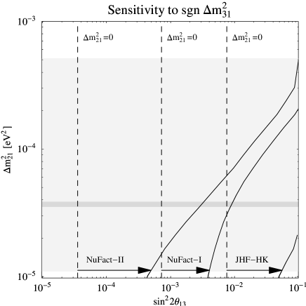
For our setups, we show the sensitivity to the sign of $\Delta m_{31}^{2}$ in Figure 14 as functions of $\sin^{2}2\theta_{13}$ and $\Delta m_{21}^{2}$. Since CP effects are proportional to $\Delta m_{21}^{2}$, or $\alpha$ in Equation (3), the $\mathrm{sgn}(\Delta m_{31}^{2})$ degeneracy disappears for small values of $\Delta m_{21}^{2}$. For large values of $\Delta m_{21}^{2}$, however, it can spoil the sign of $\Delta m_{31}^{2}$ sensitivity as much as that there can be no sensitivity at all. The figure demonstrates that, depending on the actual value of $\Delta m_{21}^{2}$ within the allowed LMA region, this sensitivity can vary over many orders of magnitude in $\sin^{2}2\theta_{13}$. For this figure, any allowed degenerate solution fitting the data is taken into account and may spoil the result if it reduces the $\chi^{2}$–function compared to the best–fit solution. In the next section, we will re–discover the $\mathrm{sgn}(\Delta m_{31}^{2})$ degeneracy in a different context, i.e., the CP measurement performance.

7 Results II: The measurement of $\delta_{\mathrm{CP}}$

The measurement of $\delta_{\mathrm{CP}}$ can be treated from two different points of view. First, one can ask for which values of $\delta_{\mathrm{CP}}$ and $\sin^{2}2\theta_{13}$ an experiment could distinguish CP violation from CP conservation, i.e., $\delta_{\mathrm{CP}}=0$ or $\delta_{\mathrm{CP}}=\pi$. This we call CP violation sensitivity. Second, one can discuss the precision of the measurement of $\delta_{\mathrm{CP}}$. In this case, we are talking about the $\delta_{\mathrm{CP}}$ precision. Since both problems are interesting and quite different from each other, we will investigate both of them.

We learned in Section 5 that the $\mathrm{sgn}(\Delta m_{31}^{2})$ degeneracy may allow different solutions at different values of $\delta_{\mathrm{CP}}$. In addition, all solutions in $\delta_{\mathrm{CP}}$ for which the energy spectrum fits the one of the true value of $\delta_{\mathrm{CP}}$ are lying on a circle from $0$ to $2\pi$. Moreover, there is little theoretical evidence for which value of $\delta_{\mathrm{CP}}$ should be preferred, i.e., any value may be equally likely. Thus, we need to define the precision of the CP measurement in a different way than the one of the $\sin^{2}2\theta_{13}$ measurement. We choose

$$\mathrm{Coverage\,in\,}\delta_{\mathrm{CP}}\equiv\frac{\sum\limits_{I}\Delta^{(I)}(\delta_{\mathrm{CP}})}{2\pi},$$ (7)

where $I$ represents all possible intervals where solutions are allowed and $\Delta^{(I)}(\delta_{\mathrm{CP}})$ the corresponding interval lengths on the $\delta_{\mathrm{CP}}$ circle at the chosen confidence level. It represents the coverage of the circle of all allowed CP phases with possible solutions, corresponding to adding the intervals of the errors in direction of the $\delta$–axis in Figure 7. If this quantity is unity, all possible values of $\delta_{\mathrm{CP}}$ are allowed, meaning that the relative measurement error is $100\%$. The smaller it is, the better is the performance of the experiment.

7.1 Impact factors on the measurement of $\delta_{\mathrm{CP}}$

Before we come to the discussion of the CP performance of the experiments, we show the main impact factors for the CP measurement. We define the impact factors for the measurement of $\delta_{\mathrm{CP}}$ similar to Equation (6) in Section 6.1 for $\sin^{2}2\theta_{13}$. Note, however, that since in this case the error of the measurement is defined as fraction of the $2\pi$ interval in Equation (7), the impact factor is also defined in terms of the relative change of this fraction. Because we will see below that a sensible CP measurement is, at least for the LMA best–fit case, only possible for the JHF-HK and NuFact-II experiments, we focus on these two experiments. In addition, the impact factors depend, of course, on the values of $\sin^{2}2\theta_{13}$ and $\delta_{\mathrm{CP}}$. In order to identify and compare the impact factors on the errors of these two experiments, we choose a parameter set which allows a quite good and comparable CP measurement in both cases, i.e., $\sin^{2}2\theta_{13}=0.01$ and $\delta_{\mathrm{CP}}=\pi/4$. In addition, we again focus on the best–fit solution ignoring degeneracies. The result of this analysis is shown in Figure 15.

Figure 15: The relative contributions of the impact factors on the measurement of $\delta_{\mathrm{CP}}$ for $\sin^{2}2\theta_{13}=0.01$ and $\delta_{\mathrm{CP}}=\pi/4$. The error sources $\xi$ are the systematical errors (“Syst”), the correlations with the large (“$\Delta m_{31}^{2}$”) and small (“$\Delta m_{21}^{2}$”) mass squared differences, the energy threshold function for neutrino factories (“$E_{\min}$”), and the uncertainty in the matter density (“$\rho$”). For the other oscillation parameters, we choose the LMA solution.

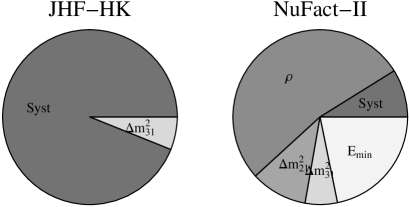
For JHF-HK we do not observe any surprising results, the measurement of $\delta_{\mathrm{CP}}$ is, as the one of $\sin^{2}2\theta_{13}$, dominated by systematics. For NuFact-II, however, the uncertainty in the matter effects takes over the main contribution to the error (impact factor about $36\%$). The importance of the matter density uncertainty on the CP measurement has, for example, been pointed out in Ref. [55]. In addition, the impact of the energy threshold function is quite large (impact factor about $15\%$).

Figure 16: The coverage in $\delta_{\mathrm{CP}}$, as defined in Equation (7), at the $2\sigma$ confidence level for the JHF-HK and NuFact-II experiments. Each bar represents the range of the sensitivity under a variation of the main impact factor (black bar) or under a variation of the luminosity (gray bar), as labeled on the left–hand side of the bar. The left vertical dash on each bar corresponds to the optimistic choice, the middle vertical dash to our standard choice, and the right vertical dash to the pessimistic choice, where the meaning of each choice is described in the main text. For the oscillation parameters, we choose the LMA solution with $\delta_{\mathrm{CP}}=\pi/4$ and $\sin^{2}2\theta_{13}=0.01$, since the two experiments perform similarly well at these parameter vales.

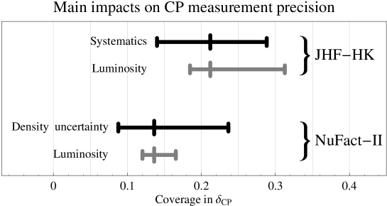
To summarize our results, Figure 16 shows the coverage in $\delta_{\mathrm{CP}}$, as defined in Equation (7), on the $2\sigma$ confidence level for the JHF-HK and NuFact-II experiments. Each bar in this figure represents the range of the coverage in $\delta_{\mathrm{CP}}$ under a variation of the main error impact or under a variation of the luminosity. The vertical dashes on each bar correspond to the optimistic choice (left), the standard choice (middle), and the pessimistic choice (right). For the luminosity, we choose twice the luminosity of our standard assumption for the optimistic choice and half the luminosity of our standard assumption for the pessimistic choice. For the main impact factors, we proceed similarly with the systematical and matter density uncertainties and double it or divide it by two. The figure shows that the JHF-HK experiment could be equally improved by increasing the luminosity and reducing the systematical errors, i.e., mainly the background uncertainties. For the NuFact-II experiment, though it is statistics dominated, the matter density uncertainty is the main impact factor and even improving the luminosity cannot compensate the need for additional knowledge about the Earth’s matter density profile.

7.2 The sensitivity to CP violation

Figure 17: The sensitivity to CP violation, as it is defined in the text, for all experiments (as labeled in the plots) at the $2\sigma$ confidence level, plotted as function of $\sin^{2}2\theta_{13}$ and $\Delta m_{21}^{2}$. The left–hand plot shows the case of $\delta_{\mathrm{CP}}=-\pi/2$ and the right–hand plot the case of $\delta_{\mathrm{CP}}=+\pi/2$. Solid curves refer to taking into account all degenerate solutions and dashed curves to taking into account the best–fit manifold only. The gray shaded regions refer to the allowed LMA region for $\Delta m_{21}^{2}$ (light gray) and the best–fit value for $\Delta m_{21}^{2}$ (dark gray). For the other oscillation parameters, we choose the LMA values.

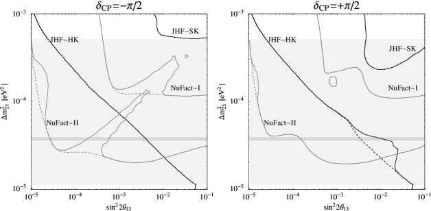
In this section, we focus on the identification of CP violation. We define the CP violation sensitivity as the ability of the experiment to distinguish CP violation from CP conservation on the $2\sigma$ confidence level, where CP conservation refers to $\delta_{\mathrm{CP}}=0$ or $\delta_{\mathrm{CP}}=\pi$, i.e., we define the overall $\chi^{2}$–function $\chi^{2}_{\mathrm{CP\,violation}}(\delta_{0})$ at the best–fit point $\delta_{0}$ as

$$\chi^{2}_{\mathrm{CP\,violation}}(\delta_{0})\equiv\min\left[\chi^{2}(\delta_{0},\delta=0),\chi^{2}(\delta_{0},\delta=\pi)\right].$$

Similarly to the $\sin^{2}2\theta_{13}$ sensitivity, we take into account all degenerate solutions by the worst case strategy. Since the CP violation sensitivity depends very much on $\sin^{2}2\theta_{13}$ and $\Delta m_{21}$, as well as the value of $\delta_{\mathrm{CP}}$ itself, we show the results in two figures. Figure 17 shows the regions of CP violation sensitivity plotted as functions of $\sin^{2}2\theta_{13}$ and $\Delta m_{21}^{2}$ for $\delta_{\mathrm{CP}}=-\pi/2$ (left plot) and $\delta_{\mathrm{CP}}=+\pi/2$ (right plot) for the different experiments (regions closed by contours to the left), where the dashed curves show what happens without taking into account degenerate solutions. First, we observe that there is no CP violation sensitivity for the JHF-SK and NuFact-I setups at the LMA best–fit value of $\Delta m_{21}^{2}$. Therefore, we will further on not discuss the measurement of $\delta_{\mathrm{CP}}$ in the context of these two experiments anymore. Second, the NuFact-II experiment performs better than the JHF-HK experiment for most values of $\Delta m_{21}^{2}$ close to the LMA solution best–fit value. However, the difference between these two experiments can be quite small even within the allowed LMA region indicated by the light gray shading. Third, the NuFact-II curve is again bend upwards for large values of $\sin^{2}2\theta_{13}$, such as it was in Figure 13, an effect coming from the matter density uncertainty. For an explanation of the degeneracy effects leading to the gap in the left–hand plot, we refer to Figure 8 and the respective discussion in Section 5 (cf., position of the “$\pi$–transit point”). The counterpart to Figure 17 is Figure 18, showing the CP violation sensitivity over $\sin^{2}2\theta_{13}$ and $\delta_{\mathrm{CP}}$ for the LMA small mass squared difference.

Figure 18: The sensitivity to CP violation, as it is defined in the text, for the JHF-HK (left–hand plot) and NuFact-II (right–hand plot) experiments at the $2\sigma$ confidence level, plotted as functions of $\sin^{2}2\theta_{13}$ and $\delta_{\mathrm{CP}}$. Solid curves refer to the case of taking into account all degenerate solutions and dashed curves to taking into account the best–fit manifold only. The gray shading marks the regions where no degenerate solutions are present at the considered confidence level. For the oscillation parameters, we choose the LMA values.

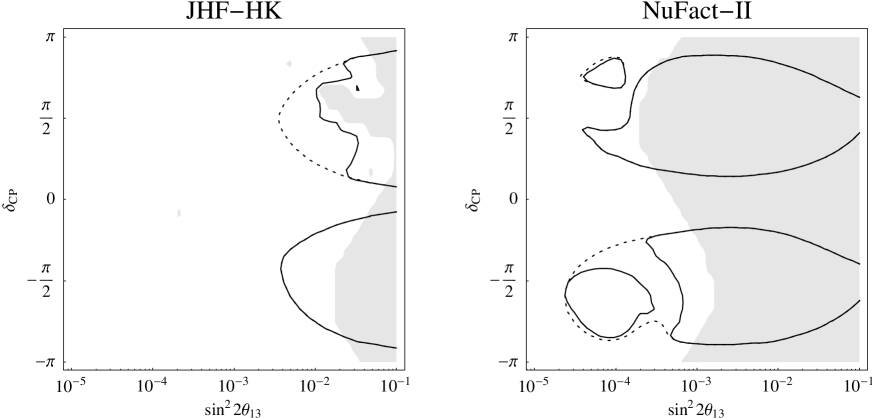
Again, the dashed lines show the case of not taking into account the degeneracies and how they make the result worse. It is obvious in these plot that there is no CP violation sensitivity around the CP conserving values $0$ and $\pi$ and the CP violation sensitivity is limited by the $\sin^{2}2\theta_{13}$ sensitivity to the left. The NuFact-II experiment performs well in a large range of $\sin^{2}2\theta_{13}$, while the JHF-HK setup is better at around the CHOOZ bound. The reason is again the matter density uncertainty, making the contours bend inwards for the NuFact-II experiment. The upper irregularity in the NuFact-II plot seems to come from a numerical coincidence, the lower irregularity can be explained by degeneracy effects similar to the last example. We also refer to Figure 8 and the respective discussion in Section 5 for an explanation.

7.3 The $\delta_{\mathrm{CP}}$ precision

In this section, we especially discuss the precision of the CP measurement, for which we introduced the quantity “Coverage in $\delta_{\mathrm{CP}}$” in Equation (7) to characterize the error on $\delta_{\mathrm{CP}}$. It is plotted in Figure 19 over $\sin^{2}2\theta_{13}$ for the NuFact-II and JHF-HK experiments, where the worst case over all values of $\delta_{\mathrm{CP}}$ is taken.

Figure 19: The coverage in $\delta_{\mathrm{CP}}$, as defined in Equation (7), plotted as function of $\sin^{2}2\theta_{13}$ for the JHF-HK and NuFact-II experiments. The curves are computed for the worst case in $\delta_{\mathrm{CP}}$. Solid curves refer to the case of taking into account all degenerate solutions, dashed curves refer to taking into account the best–fit manifold only. The light gray shading marks the region, where the NuFact-II experiment performs better and the dark gray shading the region, where the JHF-HK experiment performs better. For the oscillation parameters, we choose the LMA values.

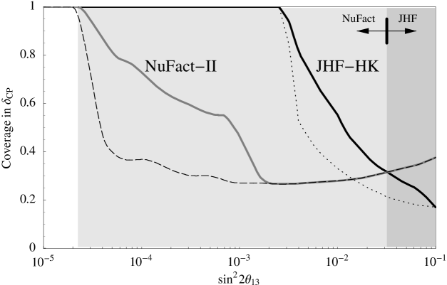
The dashed and dotted curve correspond to the case of not taking into account degenerate solutions. The NuFact-II experiment performs better in the light gray shaded region, whereas the JHF-HK experiment does better in the dark gray shaded region. However, the upward bending of the NuFact-II curve close to the CHOOZ bound again comes from the matter density uncertainty. The bump in the NuFact-II curve below about $\sin^{2}2\theta_{13}=10^{-3}$ essentially comes from the $\mathrm{sgn}(\Delta m_{31}^{2})$ degeneracy, such as the gaps in the last two plots. Here we also refer to Figure 8 and the respective discussion in Section 5 for an explanation.

8 Summary and conclusions

Figure 20: The sensitivity to $\sin^{2}2\theta_{13}$ at the 90% confidence level for all experiments and for $\Delta m_{31}^{2}=3\cdot 10^{-3}\,\mathrm{eV}^{2}$. The plot shows the effect of successively switching on the different error sources. For the oscillation parameters, the choose the LMA values but $\sin^{2}2\theta_{23}=0.8$.

Figure 21: The sensitivity to CP violation for $\delta_{\mathrm{CP}}=+\pi/2$ at the 90% confidence level, plotted as function of $\sin^{2}2\theta_{13}$. The plot shows the ranges of the sensitivity to CP violation for several values of $\Delta m_{21}^{2}$, where the top row corresponds to the lower bound, the bottom row to the upper bound, and the middle row to the best–fit value of the LMA region. If no bar is drawn for an experiment, it does not have any CP violation sensitivity. For the parameters, the choose the LMA values.

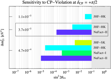
In summary, we have studied different superbeam and neutrino factory setups in order to assess and compare their physics potential for the first time on an equal footing. We have tried to model the experimental details and systematical uncertainties of each class of experiments as realistic as possible, because these are crucial to the performance of each experiment. We have performed a sophisticated statistical analysis based on event rates, including the full multi–parameter correlations among all oscillation parameters as well as the appearance of degenerate solutions. As additional input, we have assumed that the solar parameters are measured by the KamLAND experiment with a good accuracy. This comprehensive analysis is necessary to obtain reliable estimates of the physics reach of each long baseline experiment. In some cases, we have even observed a worsening of the results by orders of magnitude by switching on the sources of errors. For example, the impact of the degenerate solutions can completely destroy the sensitivity to the sign of $\Delta m_{31}^{2}$ even for a high luminosity neutrino factory, such as our NuFact-II setup.

In order to perform an appropriate comparison among the experiments, aspects equivalent for both machines have been described as by identical parameters as much as possible. We have, for example, assumed that the JHF-SK  and NuFact-I, as well as the JHF-HK and NuFact-II setups have pairwise equal running periods. For example, we have for the JHF-SK and NuFact-I experiments taken parameters which seem to be realistic for a first experiment of the considered category. For the JHF-HK and NuFact-II experiments, we have in addition chosen parameters which we consider realistic for a fully developed setup. However, such a study always depends on the current understanding or expectations. Our comparison allows moderate extrapolation if some of the parameters are different.

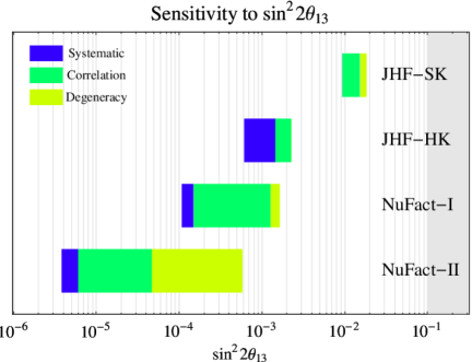
The most important aspects of our comparative results are summarized in Figures 20 and 21, where the potentials to measure $\sin^{2}2\theta_{13}$ and the CP phase $\delta_{\mathrm{CP}}$ are illustrated for the four scenarios. Figure 20 demonstrates that the $\sin^{2}2\theta_{13}$ sensitivity is reduced from an initially only statistically limited value (left edge) to a final, realistic value (right edge) including systematical errors, correlations, and degeneracies, which are successively switched on. The sensitivities of all experiments are excellent compared to the existing bounds. The JHF-SK setup can explore $\sin^{2}2\theta_{13}$ down to $\simeq 2\cdot 10^{-2}$, whereas the JHF-HK and NuFact-I setups are sensitive down to $\simeq 10^{-3}$. The NuFact-II experiment can finally constrain $\sin^{2}2\theta_{13}$ to values as small as $\simeq 5\cdot 10^{-4}$, which could be considerably improved by about one order of magnitude by a second baseline or almost maximal mixing in the atmospheric sector to lift the $(\theta_{23},\pi/2-\theta_{23})$ degeneracy.

The most important impact factors controlling the sensitivity to $\sin^{2}2\theta_{13}$ have been presented in Section 6.1. First, we have clearly seen that the JHF-SK setup is limited by statistics (i.e., the luminosity) and that systematical errors are of minor importance. Second, the JHF-HK experiment performs about one order of magnitude better and systematical uncertainties and correlations become the limiting factors. Third, the NuFact-I setup is on a purely statistical basis about one order of magnitude better than the JHF-HK experiment, but both options become rather similar after the inclusion of all errors. The largest reduction in the sensitivity comes from the correlations, i.e., especially the correlation with $\delta_{\mathrm{CP}}$. Finally, the NuFact-II setup is on a purely statistical level much better than all the other options. However, taking into account realistic errors, the final $\sin^{2}2\theta_{13}$ sensitivity limit is then only less than one order of magnitude better than that of the NuFact-I setup, especially due to the correlation and degeneracy errors. Note, however, that the sensitivity losses by the correlations and degeneracies can, in principle, be partially compensated by combining different experiments. The route to a setup such as NuFact-II will certainly involve at least one superbeam and an initial stage neutrino factory. Having different baselines and energies, these experiments in the staging scenario would help to improve the sensitivity limits by adding partially complementary information. The final sensitivity limit would then be somewhere between the systematic sensitivity limit (right edge of the black bars in Figure 20) and the full sensitivity limit (right edge of the total bars in Figure 20). From this point of view, the initial stage neutrino factory could help to improve the performance of a superbeam much better than the JHF-HK setup, since it is less limited by systematics. In this staging scenario, the NuFact-II experiment could provide improved results on the $\sin^{2}2\theta_{13}$ sensitivity by about one order of magnitude. This argumentation demonstrates that the final assessment of the physics potential of a single setup also depends on its predecessors as subsequent milestones in the staging scenario. It is therefore important to keep in mind that the physics scopes of planned experiments should be coordinated in a way that they are providing at least some complementary information.

An issue closely connected to the measurement of $\sin^{2}2\theta_{13}$, is the determination of the mass hierarchy, i.e., the measurement of $\mathrm{sgn}(\Delta m_{31}^{2})$. Surprisingly, we have found that the degeneracy between $\delta_{\mathrm{CP}}$ and the sign of ${\Delta m^{2}_{31}}$ is for all experiments the critical factor which is limiting the sensitivity. Its effects are strongest for the two superbeam experiments because of the short baselines and low energies, which means that matter effects are small. It therefore seems questionable if one can perform this measurement with superbeams at all. Not only the superbeams, but also the neutrino factory setups are limited by this degeneracy. For the largest allowed values of ${\Delta m^{2}_{21}}$ within the LMA region, it can lead to a complete loss of sensitivity. At the LMA best–fit value, the smallest value of $\sin^{2}2\theta_{13}$ for which the NuFact-I setup can determine the sign of the mass hierarchy, is about $10^{-2}$, whereas it is $5\cdot 10^{-3}$ for the NuFact-II scenario. The influence of is degeneracy could be reduced by a measurement at a second very long baseline of $\simeq 7\,000\,\mathrm{km}$ [3, 6, 9].

Figure 21 shows the sensitivity to CP violation as a function of $\sin^{2}2\theta_{13}$, which we have defined as the ability to distinguish maximal CP violation from CP conservation. Therefore, it represents the limits to CP effects for our setups. It is important to note that the minimal value of $\sin^{2}2\theta_{13}$ with sensitivity to CP violation considerably depends on the value of $\Delta m^{2}_{21}$ within the LMA range. For the LMA central value $\Delta m^{2}_{21}=3.7\cdot 10^{-5}~{}\mathrm{eV^{2}}$, only the JHF-HK and NuFact-II experiments are sensitive at all. In general, the NuFact-II experiment performs best down to $\sin^{2}2\theta_{13}\simeq 10^{-4}$ and is at the solar best–fit point about an order of magnitude better than the JHF-HK setup. For small values of $\Delta m_{21}^{2}$, however, only the JHF-HK setup is sensitive at all, which is a consequence of the short baseline and therefore the irrelevance of the matter density uncertainty. At the other end of the LMA range at the largest allowed values of $\Delta m_{21}^{2}$, all setups can measure CP violation and the JHF-HK and NuFact-II experiments perform quite similar. Nevertheless, the accuracy of the NuFact-II is slightly better because of the large number of events. The critical experimental factor limiting the CP sensitivity is, for superbeams, mainly the systematical uncertainty and, for neutrino factories, the matter density uncertainty. This also explains the surprisingly good performance of the JHF-HK experiment.

In this work, we have not discussed the optimization problem for our setups in great detail. However, for superbeams we identified the background uncertainties as the critical factor to be reduced. A potential measurement at a second, much longer baseline seems to be difficult in this case because of the huge loss in event numbers. For the neutrino factories, we have found that they would benefit from a special low energy detector for events in the range of about $4$ to $20\,\mathrm{GeV}$. In addition, a reduction in the uncertainty of the matter density would help. A second, very long baseline is probably necessary to have stronger matter effects and determine the mass hierarchy.

Acknowledgments

We wish to thank M. Messier, T. Nakaya, and C. Pe$\tilde{\mathrm{n}}$a–Garay for providing us input data and useful information. Furthermore, we thank M. Freund and N. Kaiser for useful discussions and comments.

Appendix A Calculation of event rates

The possible types of events in any detector can be classified by the flavor of the detected neutrino and its interaction type. For the experiments used in this work, these interaction types (IT) are neutral current (NC), total charged current (CC) and quasi–elastic charged current (QE) interactions. The relative abundance of these modes strongly depends on the primary energy of the incident neutrino, which means that, for example, QE interactions are only important at energies well below $10\,\mathrm{GeV}$. In this appendix, we will demonstrate how the interaction modes are implemented in the calculation of event rates.

Calculation of raw event rates

For the calculation of event rates, the first step is to compute the number of events for each IT in the fiducial mass of the detector for each neutrino flavor and energy bin. The second step is to include the detector effects coming from the insufficient knowledge used in the event reconstruction. We combine these two steps in order to obtain the differential event rate spectrum for each flavor and IT as seen by the detector, which we call a “channel”. The channels for all ITs then have to be combined in a way which takes into account that the ITs or flavors can, either because of physical reasons (e.g., the flavor–blindness of NC interactions) or because of detector effects (e.g., charge misidentification), not be measured separately.

The master formula for the differential event rate for each channel, i.e., the final flavor $f$ and the interaction type IT, is given by

$$\frac{dn_{f}^{\mathrm{IT}}}{dE^{\prime}}= N\,\sum_{f_{i}}\int\int dE\,d\hat{E}\quad\underbrace{\Phi_{f_{i}}(E)}_{\mathrm{Production}}\times$$ (8)

$$\underbrace{\frac{1}{L^{2}}P_{(f_{i}\rightarrow f)}(E,L,\rho;\theta_{23},\theta_{12},\theta_{13},\Delta m^{2}_{31},\Delta m^{2}_{21},\delta_{\mathrm{CP}})}_{\mathrm{Propagation}}\times$$

$$\underbrace{\sigma^{\mathrm{IT}}_{f}(E)k_{f}^{\mathrm{IT}}(E-\hat{E})}_{\mathrm{Interaction}}\times$$

$$\underbrace{T_{f}(\hat{E})V_{f}(\hat{E}-E^{\prime})}_{\mathrm{Detection}},$$

where $f_{i}$ is the initial flavor of the neutrino, $E$ is the incident neutrino energy, $\Phi_{f_{i}}(E)$ is the flux of the initial flavor at the source, $L$ is the baseline length, $N$ is a normalization factor, and $\rho$ is the matter density. The interaction term is composed of two factors, which are the total cross section $\sigma^{\mathrm{IT}}_{f}(E)$ for the flavor $f$ and the interaction type IT, and the energy distribution of the secondary particle $k_{f}^{\mathrm{IT}}(E-\hat{E})$ with $\hat{E}$ the energy of the secondary particle. The detector properties are modeled by the threshold function $T_{f}(\hat{E})$, coming from the the limited resolution or the cuts in the analysis, and the energy resolution function $V_{f}(\hat{E}-E^{\prime})$ of the secondary particle. Thus, $E^{\prime}$ is the reconstructed neutrino energy.

Since it is rather cumbersome to numerically solve this double integral, we use an approximation. We evaluate the integral over $\hat{E}$, where the only terms containing $\hat{E}$ are $k_{f}^{\mathrm{IT}}(E-\hat{E})$, $T_{f}(\hat{E})$, and $V_{f}(\hat{E}-E^{\prime})$, and define

$$R_{f}^{\mathrm{IT}}(E,E^{\prime})\,\epsilon_{f}^{\mathrm{IT}}(E^{\prime})\equiv\int d\hat{E}\quad T_{f}(\hat{E})\,k_{f}^{\mathrm{IT}}(E-\hat{E})\,V_{f}(\hat{E}-E^{\prime}).$$ (9)

We now approximate $R_{f}^{\mathrm{IT}}$ by the analytical expression

$$R_{f}^{\mathrm{IT}}(E,E^{\prime})=\frac{1}{\sigma_{E}\sqrt{2\pi}}\exp{\frac{(E-E^{\prime})^{2}}{2\sigma_{E}^{2}}}.$$ (10)

The values for the effective relative energy resolution $\sigma_{E}$ and the effective efficiency $\epsilon_{f}^{\mathrm{IT}}$ can be found and are explained in Appendix B.

Figure 22: Fluxes of the JHF beam (left–hand side, taken from Ref. [30]) and neutrino factory (right–hand side) at a distance of $1\,\mathrm{km}$ with a target power of $0.75\,\mathrm{MW}$, corresponding to our initial, low luminosity setups JHF-SK and NuFact-I. The anti neutrino beam spectrum for the JHF beam is different and not shown. For a neutrino factory, the anti neutrino beam has an identical flux spectrum.

Figure 23: The cross sections for the total charged current (solid curves, left–hand plot), quasi–elastic charged current (dotted curves, left–hand plot), and neutral current (right–hand plot) neutrino (black curves) and anti neutrino (gray curves) interactions [36].

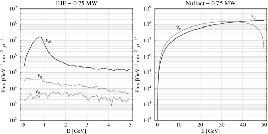
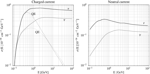
Appendix B Detector description

B.1 The JHF detector

The detector for the JHF–beam is the Super–Kamiokande (JHF-SK) detector or its $1\,\mathrm{Mt}$ version Hyper–Kamiokande (JHF-HK). We assume that the $1\,\mathrm{Mt}$ detector has the same characteristics as the Super–Kamiokande detector. This type of water Cherenkov detector has an excellent capability to identify electrons and muons based on the topology of the Cherenkov ring. Furthermore, the lepton momentum can be measured with a high precision [15].

Within each considered setup, the signal events are given by $\nu_{\mu}$ and $\nu_{e}$ CC interactions. The backgrounds are the $\nu_{\mu}$ NC events and the $\nu_{e}$ CC events already contained in the beam. Another source of backgrounds for the appearance measurement is the misidentification of muon neutrinos as electron neutrinos. The background rejection factors and the signal efficiencies are taken from Table 2 in Ref. [15]. They are assumed to be constant, which should be a reasonable approximation.

Disappearance
Signal	$0.9\otimes({\nu_{\mu}\rightarrow\nu_{\mu}})_{\mathrm{QE}}$
Background	$0.0056\otimes({\nu_{\mu}\rightarrow\nu_{x}})_{\mathrm{NC}}$
Appearance
Signal	$0.505\otimes({\nu_{\mu}\rightarrow\nu_{e}})_{\mathrm{CC}}$
Background	$0.0056\otimes({\nu_{\mu}\rightarrow\nu_{x}})_{\mathrm{NC}}$	$3.3\cdot 10^{-4}\otimes({\nu_{\mu}\rightarrow\nu_{\mu}})_{\mathrm{CC}}$
Beam background	$0.505\otimes({\nu_{e}\rightarrow\nu_{e}})_{\mathrm{CC}}$	$0.505\otimes({\bar{\nu}_{e}\rightarrow\bar{\nu}_{e}})_{\mathrm{CC}}$

Table 2: The efficiencies for the signals and backgrounds of the JHF-SK and JHF-HK experiments.

Since a water Cherenkov detector is only sensitive to leptons, there is no measurement of the hadronic energy deposition of a neutrino interaction. Therefore, the analysis of the energy spectrum has to be constrained to the QE event sample. The energy resolution for this sample is shown in Figure 24 (filled histogram).

Figure 24: The energy resolution of the $\nu_{\mu}$ events for the JHF–beam (figure taken from Ref. [15]). The filled histogram corresponds to the QE events and the open histogram to the non–QE events.

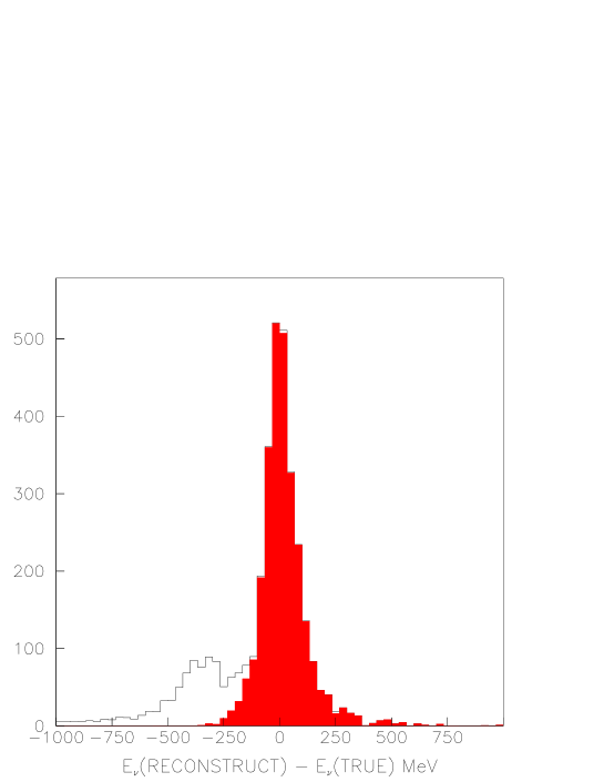
The accuracy of the energy reconstruction is limited by the Fermi–motion of the nucleons, inducing a width of about $80-100\,\mathrm{MeV}$ [30], as it can be also read off Figure 24. The distribution is, up to very good accuracy, Gaussian [30]. The Fermi–motion is energy independent and causes by far the largest error in the energy reconstruction. We use a constant width of $85\,\mathrm{MeV}$ in our analysis, i.e., $\sigma_{E}=0.085\,\mathrm{GeV}$, and we have checked that the results of the JHF-HK experiment depend only very little on this width in the range of about $80-100\,\mathrm{MeV}$. For the JHF-SK setup, the energy resolution is not important since the statistics is too low to extract spectral information.

In order to use the spectral information, we separate the signal event samples into QE events and non–QE events. In the disappearance channel, there are enough events to completely discard the non-QE events, as it is done in [15]. For the appearance channel, we adopt the following strategy in order to optimally exploit the information in the data: We use the total number of all CC events in the range $0.4-1.2\,\mathrm{GeV}$, as well as the QE spectrum with a free normalization in order to avoid a double counting of QE events. This separation of rates and spectra is a well-known technique, such as it is used in the solar analysis of Super–Kamiokande in Ref. [51].

B.2 The NuFact detector

The detector we consider for a neutrino factory is a magnetized iron calorimeter, similar to the MINOS [56] or MONOLITH [57] detectors. This detector type allows to measure both the leptonic and hadronic energy deposition. In addition, the background rejection for NC events is very good and the accuracy of the muon charge measurement with the magnetic field of $\sim 1\,\mathrm{T}$ is very high. Figure 25 shows the energy resolution $\sigma_{E}$, i.e., the width of a Gaussian energy distribution curve, plotted as function of the neutrino energy $E_{\nu}$.

Figure 25: The energy resolution $\sigma_{E}$ of $\nu_{\mu}$ events for a NuFact detector. The solid black curve represents the energy resolution used in this work. The thick dashed curve shows the resolution for the MINOS detector [56], assuming that the neutrino energy is equally distributed between hadrons and muons. The thin dashed curves show the hypothetical resolution of MINOS, if the neutrino energy went either only to hadrons (upper curve) or muons (lower curve) only. The gray–shaded area indicates the region which is cut off by the bin width used in our work.

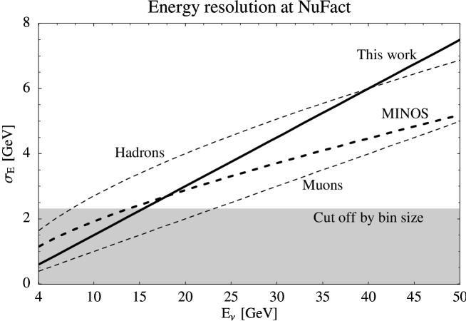
The Gaussian modeling of the energy resolution should be fairly good, especially since the non–Gaussian tails are expected to be small [56]. The figure shows the curves for our analysis (thick solid curve), the MINOS detector for an equal distribution of the energy between hadrons and muons (thick dashed curve), and the MINOS detector for the hypothetical case of all neutrino energy going to hadrons (upper thin dashed curve) or muons (lower thin dashed curve) only. As it can be seen from this figure, we use the linear, quite conservative approximation $\sigma_{E}=0.15\,E_{\nu}$ of the energy resolution, since below $15\,\mathrm{GeV}$ the energy resolution is constrained by the bin size in our model. In order to have a more accurate modeling of the problem and a better sensitivity to physical quantities, one could even use smaller energy bins at low energies together with more accurate parameterization for the energy resolution.

Another important issue for the NuFact detector is the minimum muon momentum cut together with the background level. There existe essentially two detailed studies of detectors [7, 58], which find slightly different results. One strategy is to optimize the signal to noise ratio, which is especially important for poor statistics, i.e., a rather small number of events. The authors of Ref. [58], for example, use a minimum muon momentum cut at $7.5\,\mathrm{GeV}$ and a $q_{t}$ cut at $1\,\mathrm{GeV}$. These tight cuts result in a low wrong-sign muon background level of $\sim 10^{-6}$ and a small efficiency below $10\,\mathrm{GeV}$. Another possibility is to use a lower muon momentum cut at $4\,\mathrm{GeV}$, such as it is done in Ref. [7]. This results in a much higher background level of $\sim 10^{-4}$ and better efficiencies at low and high energies. Since a larger number of events in the low–energy regime is for the planned precision measurements more important than maximum background suppression, we follow an intermediate strategy, interpolating between those two cases. We use an efficiency linearly rising from zero to one between $4\,\mathrm{GeV}$ and $20\,\mathrm{GeV}$ together with an intermediate background level of $10^{-5}$. This corresponds to a detector in between the setups studied in Refs. [7, 58]. In Refs. [4, 58] it is also shown and clearly stated that the S/N ratio does not strongly change for a cut on the muon momentum at more than $5\,\mathrm{GeV}$ and a cut on $q_{t}$ at more than $0.5\,\mathrm{GeV}$.

Figure 26: The signal efficiencies as functions of the neutrino energy used for our NuFact setups (thick black curves). The gray histograms are taken from Ref. [4]. The thin curves represent the best linear fits between $0$ and $20\,\mathrm{GeV}$ to the gray histograms.

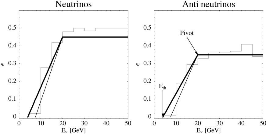
In Figure 26, the efficiency functions used in this work are plotted as functions of the energy as thick curves, whereas the gray histograms correspond to the efficiency functions used in Ref. [4]. The thin curves represent linear interpolations to these histograms. In this case, the efficiencies are zero at $7.5\,\mathrm{GeV}$ and rise to their final values at $20\,\mathrm{GeV}$.

The signal at a neutrino factory consists of the $\nu_{\mu}$ disappearance and the wrong-sign muon appearance signal. The backgrounds for these signals are a certain fraction of the NC events for all flavors and the misidentified fraction of the $\nu_{\mu}$–CC events. The values used in this work are shown in Table 3.

Disappearance – $\mu^{-}$ stored
Signal	$0.45\otimes({\nu_{\mu}\rightarrow\nu_{\mu}})_{\mathrm{CC}}$
Background	$10^{-5}\otimes({\nu_{\mu}\rightarrow\nu_{x}})_{\mathrm{NC}}$
Disappearance – $\mu^{+}$ stored
Signal	$0.35\otimes({\bar{\nu}_{\mu}\rightarrow\bar{\nu}_{\mu}})_{\mathrm{CC}}$
Background	$10^{-5}\otimes({\bar{\nu}_{\mu}\rightarrow\bar{\nu}_{x}})_{\mathrm{NC}}$
Appearance – $\mu^{-}$ stored
Signal	$0.45\otimes({\bar{\nu}_{e}\rightarrow\bar{\nu}_{\mu}})_{\mathrm{CC}}$
Background	$5\cdot 10^{-6}\otimes({\nu_{\mu}\rightarrow\nu_{x}})_{\mathrm{NC}}$	$5\cdot 10^{-6}\otimes({\nu_{\mu}\rightarrow\nu_{\mu}})_{\mathrm{CC}}$
Appearance – $\mu^{+}$ stored
Signal	$0.35\otimes({\nu_{e}\rightarrow\nu_{\mu}})_{\mathrm{CC}}$
Background	$5\cdot 10^{-6}\otimes({\bar{\nu}_{\mu}\rightarrow\bar{\nu}_{x}})_{\mathrm{NC}}$	$5\cdot 10^{-6}\otimes({\bar{\nu}_{\mu}\rightarrow\bar{\nu}_{\mu}})_{\mathrm{CC}}$

Table 3: The high energy efficiencies for the signals and backgrounds of the NuFact-I and NuFact-II experiments.

These high energy efficiencies are taken from Ref. [4] and the low energy efficiencies from Ref. [7]. The background level is an interpolation between the two mentioned references to take into account the lower muon momentum cut. The high energy efficiencies of Ref. [7] are $\sim 50\%$ for both neutrinos and anti neutrinos, which are considerably larger than the ones used in this work.

In order to illustrate the effects of the energy threshold function, which is determined by the muon momentum cut, we show in Figure 27 the dependence of our results for $\delta_{\mathrm{CP}}$ and $\sin^{2}2\theta_{13}$ on the muon momentum cut $E_{th}$. We parameterize the threshold function by keeping the point at $20\,\mathrm{GeV}$ in Figure 26, labeled as pivot, fixed and moving the point labeled by $E_{th}$.

Figure 27: The allowed ranges in $\sin^{2}2\theta_{13}$ (left–handed panel) and $\delta_{\mathrm{CP}}$ (right–handed panel) as functions of the threshold energy $E_{th}$ for the starting values $\sin^{2}2\theta_{13}=10^{-3}$, $\delta_{\mathrm{CP}}=\pi/4$, and the LMA solution. The black solid curves show the results at the $90\%$ CL used in this work. The shading marks the $1\,\sigma$ (dark gray), $2\,\sigma$ (medium gray), and $3\,\sigma$ (light gray) allowed ranges. The left vertical lines corresponds to the black solid curves in Figure 26 and the right vertical lines to the thin black curves in Figure 26. The shaded ranges are the results of two–dimensional fits of $\sin^{2}2\theta_{13}$ and $\delta_{\mathrm{CP}}$, which means that multi–parameter correlations are neglected in this plot.

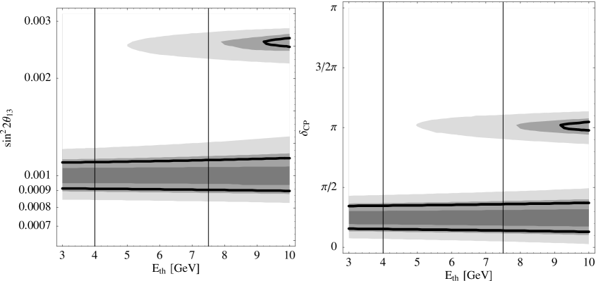
In Figure 27 the allowed ranges in $\delta_{\mathrm{CP}}$ (right–handed panel) and in $\sin^{2}2\theta_{13}$ (left–handed panel) are shown as functions of the threshold energy $E_{th}$. The starting values used are the LMA values, $\delta_{\mathrm{CP}}=\pi/4$, and $\sin^{2}2\theta_{13}=10^{-3}$. The allowed ranges are determined by projection of the two–dimensional $\delta_{\mathrm{CP}}-\sin^{2}2\theta_{13}$ allowed region onto the $\delta_{\mathrm{CP}}$ and $\sin^{2}2\theta_{13}$ axis, respectively. The gray shading corresponds to the $1\,\sigma$ (dark gray), $2\,\sigma$ (medium gray), and $3\,\sigma$ (light gray) allowed ranges. The thick black curves represents the $90\%$ CL used in this work. The left vertical lines mark the value for the threshold function used in this work and corresponds to the thick black curves in Figure 26. The right vertical lines mark the value for the threshold function given by the thin black curves in Figure 26, which very closely approximates the gray histogram with the efficiencies used in Ref. [4]. Figure 28 clearly demonstrates that changing the threshold value mainly changes the confidence level at which the second solution of the $(\delta,\theta_{13})$ ambiguity appears. For the $90\%$ CL used in this work, this dependency is obviously very small, since neither does the range around the true solution increase much, nor does the second solution appear at the $90\%$ CL.

Figure 28: The $\Delta\chi^{2}$–functions of a full analysis, as they are used throughout this work, as functions of $\sin^{2}2\theta_{13}$ (left–handed panel) and $\delta_{\mathrm{CP}}$ (right–handed panel). The used parameter values are $\sin^{2}2\theta_{13}=10^{-3}$, $\delta_{\mathrm{CP}}=\pi/4$, and the LMA solution. The solid curves correspond to the thick black curves in Figure 26 and the dashed curves correspond to the thin black curves in Figure 26. The horizontal lines show the confidence level used in this work.

This can be also seen in Figure 28, where the results of a full analysis, as used throughout this work, are shown. It shows $\Delta\chi^{2}$ as function of $\sin^{2}2\theta_{13}$ (left–handed panel) and $\delta_{\mathrm{CP}}$ (right–handed panel). The solid curves show the results obtained with $E_{th}=4\,\mathrm{GeV}$, as used in this work, and indicated by the thick black curves in Figure 26. The dashed curves represent the result obtained with $E_{th}=7.5\,\mathrm{GeV}$, corresponding to the thin black curves in Figure 26. The solid and dashed curves are practically identical around the true solution. Only at the degenerate solution from the $(\delta,\theta_{13})$ ambiguity a noteworthy difference occurs. It results in a lowering of the minimum $\Delta\chi^{2}$ of the degenerate solution from $9.3$ to $3.8$, which means that the degenerate solution now appears at the $2\,\sigma$ level instead of the $3\,\sigma$ confidence level. Still, it does not appear at the $90\%$ CL used in this work. In general, the qualitative impact of the threshold value is small and its quantitative influence strongly depends on the selected confidence level. In both cases, $E_{th}=4\,\mathrm{GeV}$ and $E_{th}=7.5\,\mathrm{GeV}$, the degenerate solution is present, but at different confidence levels. Furthermore, a change of the oscillation parameters, such as especially of ${\Delta m^{2}_{21}}$, can change the confidence level at which the degenerate solution appears. Finally, it is not yet clear which strategy – low momentum cut with a high background level or vice versa – will be most efficient for the quantities of interest. This discussion shows that more detailed studies of detector properties and detector concepts will be needed in order to optimally balance the threshold versus background level for optimum sensitivities.

Appendix C Statistics and the treatment of systematical errors

In order to evaluate the physics potential of each setup, we compute spectral event rate spectra for a certain set of (true) oscillation parameters $\lambda_{0}$ and compare it to a parameter set $\lambda$ by a $\chi^{2}$–analysis. In this paper, this analysis aims to obtain statistically reliable statements about possible measurements of $\theta_{13}$, $\mathrm{sgn}({\Delta m^{2}_{31}}^{2})$, and $\delta_{\mathrm{CP}}$. The fit to the data is performed including all available information, i.e., using all types of signals. These are the appearance and disappearance channels for the neutrino beam and appearance and disappearance channels for the anti neutrino beam (which are not available for the JHF-SK setup). In this appendix, we refer to the types of signals by $\alpha$. It turns out to be extremely important to include the disappearance signals and the energy information in the analysis, although we are only interested in the measurements of $\theta_{13}$, $\mathrm{sgn}({\Delta m^{2}_{31}}^{2})$, and $\delta_{\mathrm{CP}}$. Since these measurements require excellent knowledge about the atmospherical oscillation parameters ${\Delta m^{2}_{31}}$ and $\theta_{23}$, and the precision from other experiments, such as the MINOS experiment [39], is not comparable to the one of the experiments described in this work, the experiments themselves will supply this knowledge. In addition, the spectral information in the appearance channels helps to improve the resolution of degeneracies (e.g., see Figures 5 and 6).

We use the full set of the standard three–flavor oscillation parameters, which are ${\Delta m^{2}_{21}}$, $\theta_{12}$, ${\Delta m^{2}_{31}}$, $\theta_{23}$, $\theta_{13}$, and $\delta_{\mathrm{CP}}$. The appearance probability in Equation (2), however, only depends on the solar parameter product $\pi_{\mathrm{sol}}\equiv\sin 2\theta_{12}\cdot{\Delta m^{2}_{21}}$. Therefore, we use this product $\pi_{\mathrm{sol}}$ as the relevant parameter reducing the number of oscillation parameters to five. In summary, we call our set of oscillation parameters $\lambda\equiv\{\pi_{\mathrm{sol}},{\Delta m^{2}_{31}},\theta_{23},\theta_{13},\delta_{\mathrm{CP}}\}$. This is the only approximation introduced for the treatment of the transition probabilities.

As basis for a statistical analysis, we use the standard $\chi^{2}$-function for Poissonian distributed quantities, such as given in [28]:

$$\chi^{2} = \sum_{i=1}^{b}\left(2[\langle x_{i}\rangle-x_{i}]+2\thinspace x_{i}\log\frac{x_{i}}{\langle x_{i}\rangle}\right).$$ (11)

Here, $b$ is the number of bins, $x_{i}$ is the number of events in the $i$th bin, and $\langle x_{i}\rangle$ is the expectation value of the number of events in the $i$th bin. Though this method is in this form quite simple, it is not easy to include systematical errors and external information in a consistent and simple way. To implement systematical errors and external information, we parameterize the considered problem linearly and restrict it to a certain interval given by its uncertainty.

For each bin $i$, the total number of events is the sum of signal and background events, i.e.,

$$x_{i}=s_{i}+b_{i},$$ (12)

where $s_{i}$ is the number of signal events and $b_{i}$ is the number of background events, such as it is defined in the previous appendix. We introduce systematical errors in $x_{i}$ and $b_{i}$ by modifying the signal $s_{i}^{0}$ and background $b_{i}^{0}$ raw event rates from the previous appendix by

$$s_{i}=s_{i}(n_{s},t_{s})=s_{i}^{0}\,(1+n_{s}+t_{s}\cdot E_{i}/(E_{\mathrm{max}}-E_{\mathrm{min}}))\,,$$

$$b_{i}=b_{i}(n_{b},t_{b})=b_{i}^{0}\,(1+n_{b}+t_{b}\cdot E_{i}/(E_{\mathrm{max}}-E_{\mathrm{min}})),$$ (13)

where $E_{i}$ is the average energy in the $i$th bin, $E_{\mathrm{max}}$ is the maximum energy, and $E_{\mathrm{min}}$ is the minimum energy of all bins. The auxiliary parameter $n$ is called “normalization” and describes the effect of an overall change in the magnitude of signal or background, whereas the parameter $t$ is called “tilt” and describes a linear distortion in the spectral shape of the signal or background. This distortion can come from limited knowledge of the background or an energy calibration error. The total number of events in the $i$–th bin $x_{i}$ now becomes

$$x_{i}=x_{i}(n_{s},t_{s},n_{b},t_{b})=s_{i}(n_{s},t_{s})+b_{i}(n_{b},t_{b}).$$ (14)

Note that $n^{\alpha}_{s}$, $t^{\alpha}_{s}$, $n^{\alpha}_{b}$, and $t^{\alpha}_{b}$ are independent parameters and we have a different set of these four parameters for each channel $\alpha$. Finally, the $\chi^{2}$–function does not only depend on the five oscillation parameters and the matter density $\rho$, but also on the auxiliary parameters $n^{\alpha}_{s},t^{\alpha}_{s},n^{\alpha}_{b}$ and $t^{\alpha}_{b}$:

$$\chi^{2}_{\alpha}=\chi^{2}_{\alpha}(\lambda,\rho;n^{\alpha}_{s},t^{\alpha}_{s},n^{\alpha}_{b},t^{\alpha}_{b})\,.$$ (15)

In order to implement the uncertainties of the auxiliary parameters, we assume that the values of $n^{\alpha}_{s}$, $t^{\alpha}_{s}$, $n^{\alpha}_{b}$, $t^{\alpha}_{b}$ are known with some accuracy $\sigma$, i.e., are distributed in a Gaussian way with the mean value $0$ and the standard deviation $\sigma$. The standard deviation $\sigma$ corresponds to the systematical uncertainty of these quantities, whereas the statistical uncertainty is already taken into account by the form of the $\chi^{2}$-function in Equation (11). Because of the likelihood principle, i.e., the $\chi^{2}$–function in terms of the likelihood $\mathcal{L}$ given by $-2\log\mathcal{L}$, the restriction to a Gaussian with mean $\mu$ and standard deviation $\sigma$ leads to the additional term $(x-\mu)^{2}/\sigma^{2}$ in the $\chi^{2}$-function. For each of the auxiliary parameters, we include this additional term and minimize with respect to it:

$$\hat{\chi}^{2}_{\alpha}(\lambda,\rho)=\min_{n^{\alpha}_{s},t^{\alpha}_{s},n^{\alpha}_{b},t^{\alpha}_{b}}\left(\chi^{2}_{\alpha}(\lambda,\rho;n^{\alpha}_{s},t^{\alpha}_{s},n^{\alpha}_{b},t^{\alpha}_{b})+\frac{(n^{\alpha}_{s})^{2}}{\sigma^{2}_{n^{\alpha}_{s}}}+\frac{(t^{\alpha}_{s})^{2}}{\sigma^{2}_{t^{\alpha}_{s}}}+\frac{(n^{\alpha}_{b})^{2}}{\sigma^{2}_{n^{\alpha}_{b}}}+\frac{(t^{\alpha}_{b})^{2}}{\sigma^{2}_{t^{\alpha}_{b}}}\right).$$ (16)

In this equation, $\hat{\chi}^{2}_{\alpha}(\lambda,\rho)$ is the marginalized (with respect to $n^{\alpha}_{s},t^{\alpha}_{s},n^{\alpha}_{b},t^{\alpha}_{b}$) distribution of $\chi^{2}_{\alpha}$. With this step, we have eliminated a part of the nuisance parameters which have been assumed to be fully uncorrelated. In principle, it is also possible to perform this marginalization for all nuisance parameters and the projection onto the parameter of interest $\eta$ in one step. However, it saves computation time to use a two–step method, since the first step does not require the re–computation of oscillation probabilities. For both steps, we use a fast “direction set” method to find the minimum. The algorithm and its implementation in C are taken from [59, pp. 420–425]. The advantages of using this minimization algorithm are its high speed and its excellent accuracy compared to a brute force grid–based methods. Furthermore, it does not require the computation of derivatives of the function to be minimized, because derivatives of numerical functions are very unstable and quite slow to be computed. However, such a heuristics does not completely run independently without using some expert knowledge from the field.

Similarly to the inclusion of the normalizations and tilts, we can use the same procedure for the matter density $\rho$, where the mean value and uncertainty are taken from seismic wave measurements, and the solar parameters $\pi_{\mathrm{sol}}$, where the mean value and uncertainty are expected to be measured by the KamLAND experiment. Finally, we project onto the parameter of interest $\eta$ in order to obtain

$$\chi^{2}_{\mathrm{F}}(\eta)=\min_{\bar{\lambda},\rho}\left(\sum_{\alpha}\hat{\chi}^{2}_{\alpha}(\lambda,\rho)+\frac{(\rho-\rho^{0})^{2}}{\sigma^{2}_{\rho}}+\frac{(\pi_{\mathrm{sol}}-\pi^{0}_{\mathrm{sol}})^{2}}{\sigma^{2}_{\pi_{\mathrm{sol}}}}\right),$$ (17)

where $\bar{\lambda}$ refers to the set of oscillation parameters without $\eta$. We use for all setups [31, 32, 34]

$$\sigma_{\pi_{\mathrm{sol}}}=0.15\,\pi_{\mathrm{sol}}^{0}\quad\mathrm{and}\quad\sigma_{\rho}=0.05\,\rho^{0}.$$

The $1\sigma$ uncertainties for the auxiliary parameters are for all setups given in Table 4. In our analysis, it turns out that for all these errors a variation by a factor of two does not affect the final results very much – with the exception of $\sigma_{n_{b}}$ for the appearance channels of the JHF-HK setup. For a more comprehensive discussion, we refer to Sections 6.1 and 6.2.

	$\sigma_{n_{s}}$	$\sigma_{t_{s}}$	$\sigma_{n_{b}}$	$\sigma_{t_{b}}$
Disappearance – NuFact	0.01	0.05	0.05	0.05
Appearance – NuFact	0.01	0.05	0.2	0.05
Disappearance – JHF	0.05	0.025	0.2	0.025
Appearance – JHF	0.05	0.025	0.05	0.05

Table 4: Systematical uncertainties for our setups from Refs. [57, 60, 58, 29] for the neutrino factory experiments and from Refs. [15, 35, 61, 62, 63] for the JHF experiments.

The error or sensitivity for the parameter of interest $\eta$ is defined as the range of $\eta$ where $\chi^{2}_{\mathrm{F}}(\eta)\leq\chi^{2}_{\mathrm{crit}}$. Here $\chi^{2}_{\mathrm{crit}}$ is determined by the $\chi^{2}$–distribution with one degree of freedom, i.e., $\chi^{2}_{\mathrm{crit}}=1$ on $1\sigma$ confidence level, $\chi^{2}_{\mathrm{crit}}=2.71$ for $90\%$ confidence level, and $\chi^{2}_{\mathrm{crit}}=4$ for $2\sigma$ confidence level. Specifically, the sensitivity limit for $\eta=\sin^{2}2\theta_{13}$ is defined by $\chi^{2}_{\mathrm{F}}(\eta,\eta^{0}=0)$, the CP violation sensitivity is given by $\min\left\{\chi^{2}_{\mathrm{F}}(\delta_{\mathrm{CP}},\delta_{\mathrm{CP}}^{0}=0),\chi^{2}_{\mathrm{F}}(\delta_{\mathrm{CP}},\delta_{\mathrm{CP}}^{0}=\pi)\right\}$, and the sensitivity to the sign of ${\Delta m^{2}_{31}}$ is obtained by minimizing the $\chi^{2}$–function over all possible parameter sets with the sign of ${\Delta m^{2}_{31}}$ opposite to the sign at the starting point $\lambda^{0}$.

References

- [1] A. D. Rujula, M. B. Gavela, and P. Hernandez, Nucl. Phys. B547, 21 (1999), hep-ph/9811390.
- [2] V. D. Barger, S. Geer, R. Raja, and K. Whisnant, Phys. Rev. D62, 013004 (2000), hep-ph/9911524.
- [3] M. Freund, M. Lindner, S. T. Petcov, and A. Romanino, Nucl. Phys. B578, 27 (2000), hep-ph/9912457.
- [4] A. Cervera et al., Nucl. Phys. B579, 17 (2000), erratum ibid. Nucl. Phys. B593, 731 (2001), hep-ph/0002108.
- [5] V. D. Barger, S. Geer, R. Raja, and K. Whisnant, Phys. Rev. D62, 073002 (2000), hep-ph/0003184.
- [6] M. Freund, P. Huber, and M. Lindner, Nucl. Phys. B585, 105 (2000), hep-ph/0004085.
- [7] C. Albright et al. (2000), hep-ex/0008064, and references therein.
- [8] J. Burguet-Castell, M. B. Gavela, J. J. Gomez-Cadenas, P. Hernandez, and O. Mena, Nucl. Phys. B608, 301 (2001), hep-ph/0103258.
- [9] M. Freund, P. Huber, and M. Lindner, Nucl. Phys. B615, 331 (2001), hep-ph/0105071.
- [10] O. Yasuda (2001), and references therein, hep-ph/0111172.
- [11] A. Bueno, M. Campanelli, S. Navas-Concha, and A. Rubbia, Nucl. Phys. B631, 239 (2002), hep-ph/0112297.
- [12] O. Yasuda (2002), and references therein, hep-ph/0203273.
- [13] V. Barger, S. Geer, R. Raja, and K. Whisnant, Phys. Rev. D63, 113011 (2001), arXiv:hep-ph/0012017.
- [14] J. J. Gomez-Cadenas et al. (CERN working group on Super Beams) (2001), hep-ph/0105297.
- [15] Y. Itow et al. arXiv:hep-ex/0106019.
- [16] H. Minakata and H. Nunokawa, JHEP 10, 001 (2001), hep-ph/0108085.
- [17] G. Barenboim, A. De Gouvea, M. Szleper, and M. Velasco (2002), hep-ph/0204208.
- [18] G. Acquistapace et al. (CNGS Collab.) CERN-98-02.
- [19] R. Baldy et al. (CNGS Collab.) CERN-SL-99-034-DI.
- [20] J. Hylen et al. (Numi Collab.) FERMILAB-TM-2018.
- [21] K. Nakamura (K2K Collab.), Nucl. Phys. A663, 795 (2000).
- [22] M. Aoki (2002), hep-ph/0204008.
- [23] A. Para and M. Szleper (2001), hep-ex/0110032.
-
[24]
F. Dydak, Tech.
Rep., CERN (2002),
http://home.cern.ch/dydak/oscexp.ps. - [25] M. Szleper and A. Para (2001), hep-ex/0110001.
- [26] S. Geer, Phys. Rev. D57, 6989 (1998), hep-ph/9712290.
[27]
N. Holtkamp and
D. Finley,
Tech. Rep., FNAL
(2002),
http://www.fnal.gov/projects/muon_collider/nu-factory/nu-factory.html. -
[28]
Particle Data Group, D.E. Groom et al.,
Eur. Phys. J. C 15,
1 (2000),
http://pdg.lbl.gov/. - [29] A. Blondel et al., Nucl. Instrum. Meth. A451, 102 (2000).
- [30] T. Nakaya, private communication.
[31]
V. Barger,
D. Marfatia, and
B. Wood,
Phys. Lett. B498,
53 (2001),
hep-ph/0011251. - [32] M. C. Gonzalez-Garcia and C. Pea-Garay, Phys. Lett. B527, 199 (2002), hep-ph/0111432.
- [33] M. Freund, Phys. Rev. D64, 053003 (2001), hep-ph/0103300.
- [34] R. J. Geller and T. Hara (2001), hep-ph/0111342.
- [35] M. D. Messier, Ph.D. thesis, Boston University (1999).
- [36] M. D. Messier, private communication.
- [37] T. Kitagaki et al., Phys. Rev. Lett. 49, 98 (1982).
- [38] E. A. Paschos (2002), hep-ph/0204138.
- [39] V. D. Barger et al., Phys. Rev. D65, 053016 (2002), hep-ph/0110393.
- [40] K. Scholberg (SuperKamiokande Collab.) (1999), hep-ex/9905016.
- [41] S. Fukuda et al. (Super-Kamiokande Collab.), Phys. Rev. Lett. 85, 3999 (2000), hep-ex/0009001.
- [42] M. Ambrosio et al. (MACRO Collab.), Phys. Lett. B434, 451 (1998), hep-ex/9807005.
[43]
S. Geer, and
K. Whisnant,
Phys. Rev. D61,
053004 (2000),
hep-ph/9906487. - [44] L. Wolfenstein, Phys. Rev. D17, 2369 (1978).
- [45] L. Wolfenstein, Phys. Rev. D20, 2634 (1979).
- [46] S. P. Mikheev and A. Y. Smirnov, Sov. J. Nucl. Phys. 42, 913 (1985).
- [47] S. P. Mikheev and A. Y. Smirnov, Nuovo Cim. C9, 17 (1986).
- [48] V. Barger, D. Marfatia, and K. Whisnant, Phys. Rev. D65, 073023 (2002), hep-ph/0112119.
- [49] M. C. Gonzalez-Garcia and M. Maltoni (2002), hep-ph/0202218.
- [50] M. Maltoni, Nucl. Phys. Proc. Suppl. 95, 108 (2001), hep-ph/0012158.
- [51] J. N. Bahcall, M. C. Gonzalez-Garcia, and C. Pea-Garay, JHEP 04, 007 (2002), hep-ph/0111150.
- [52] C. Pea-Garay, private communication.
- [53] M. Apollonio et al. (Chooz Collab.), Phys. Lett. B466, 415 (1999), hep-ex/9907037.
- [54] K. Dick, M. Freund, P. Huber, and M. Lindner, Nucl. Phys. B588, 101 (2000), hep-ph/0006090.
- [55] L.-Y. Shan, B.-L. Young, and X.-m. Zhang hep-ph/0110414.
- [56] E. Ables et al. (MINOS) FERMILAB-PROPOSAL-P-875.
- [57] N. Y. Agafonova et al. (MONOLITH Collab.) LNGS-P26-2000.
- [58] A. Cervera, F. Dydak, and J. Gomez Cadenas, Nucl. Instrum. Meth. A451, 123 (2000).
- [59] W. H. Press, S. A. Teukolsky, W. T. Vetterling, and B. P. Flannery, Numerical Recipes in C (Cambridge University Press, 1995).
- [60] A. Geiser, private communication.
- [61] K. Ishihara, Ph.D. thesis, University of Tokyo (1999).
- [62] K. Okumura, Ph.D. thesis, University of Tokyo (1999).
- [63] W. Flanagan, Ph.D. thesis, University of Hawaii (1997).