Solar neutrino measurements in Super–Kamiokande–I

Abstract

The details of Super–Kamiokande–I’s solar neutrino analysis are given. Solar neutrino measurement in Super–Kamiokande is a high statistics collection of ⁸B solar neutrinos via neutrino-electron scattering. The analysis method and results of the 1496 day data sample are presented. The final oscillation results for the data are also presented.

I Introduction

Super–Kamiokande [Super–K, SK] is an imaging water Cherenkov detector, which detects ⁸B solar neutrinos by electron scattering. Due to its unprecedented fiducial size of 22.5 kilotons, Super–K has the advantage of making the current highest statistics measurements of solar neutrinos. It enables us to determine, with high precision, measurements of the solar neutrino flux, energy spectrum, and possible time variations of the flux.

Super–K started taking data in April 1996, and the solar neutrino results of the first phase of SK, which ended in July 2001 and is henceforth referred to as “SK–I,” are described in this paper. In Section II and Section III, details of the SK detector and its simulation are given. After the event reconstruction method, detector calibration, and sources of background are described in Sections IV,  V, and VI respectively, the data analysis method and results are described in SectionVII and VIII. Finally, in Section IX the solar neutrino oscillation analysis is discussed.

II Super–Kamiokande detector

II.1 Detector outline

As has been discussed in much greater detail elsewhere sk_detector , the Super–Kamiokande detector consists of about 50000 tons of ultra-pure water in a stainless steel cylindrical water tank with 11146 20-inch photomultiplier tubes [PMT’s] in the inner detector [ID] and 1885 8-inch PMT’s in the outer detector [OD]. The diameter and height of the SK tank are 39.3 meters and 41.4 meters, respectively. The coordinates of the SK tank are defined in Figure 1. In the inner detector, the active photodetector coverage is 40.4% while the remainder is covered with black, polyethylene terephthalate sheets, generally referred to simply as “black sheet.” Signals from PMT’s are sent through an electronics chain which can measure both the arrival time of Cherenkov photons as well as the amount of charge they liberate from the phototubes’ photocathodes.

Figure 1: Coordinates of the Super–Kamiokande detector. The Z-axis is defined as the upward direction, pointing away from the center of the earth.

The Super–K detector is located 1000 meters underground (2700 meters of water equivalent) in Kamioka Observatory, deep within the Kamioka mine in Gifu Prefecture, Japan. The Observatory is owned and operated by the Institute for Cosmic Ray Research [ICRR], a division of the University of Tokyo. The detector’s latitude and longitude are 36^∘ 25’ N and 137^∘18’ E, respectively. Compared to ground level, the intensity of muons is reduced by about $10^{-5}$ at the depth of the SK detector, and yielding a downward-going muon rate through the detector of about 2 Hz.

As radon concentrations in the Kamioka mine air can exceed 3000 Bq/m³ during the summer season, there are air-tight doors between the Super–K detector area and the mine tunnel. The excavated, domed area above the cylindrical water tank, called the “SK dome,” is coated with radon-resistant plastic sheets to prevent radon in the surrounding rock from entering the air above the detector. Fresh air from outside the mine is continuously pumped into the SK dome area at the rate of $5\sim 12$ m³/minute. As a result, the typical radon concentration in the SK dome air is 20$\sim$30 mBq/m³.

As we will see in Section VI, radon can lead to background events in the solar neutrino data set. In order to keep radon out of the detector itself, the SK tank is tightly sealed. Radon-reduced air, produced by a special air purification system in the mine, is continuously pumped into the space above the water surface inside the SK tank, maintaining positive pressure. The radon concentration of this radon-reduced air is less than 3 mBq/m³.

Finally, the purified water in the SK tank is continuously circulated through the water purification system in the mine at the rate of about 35 tons/hour. This means that the entire 50 kiloton water volume of the detector is passed through the filtration system once every two months or so.

II.2 Photomultiplier tubes

The PMT’s used in the inner part of SK are the 20-inch diameter PMT’s developed by Hamamatsu Photonics K.K. in cooperation with members of the original Kamiokande experiment pmt1 . Detailed descriptions of these PMT’s, including their quantum efficiencies [Q.E.], single photo-electron distributions, timing resolutions, and so on, may be found elsewhere pmt2 .

Good timing resolution for light arrival at each PMT is essential for event reconstruction. It is around 3 nsec for single photo-electron light levels.

The dark noise rate of the PMT’s is measured to be around 3.5 kHz on average and it was stable over the SK–I data taking period as shown in Figure 2(a). The number of accidental hits caused by this dark noise is estimated to be about 2 hits in any 50 nsec time window. For the solar neutrino analysis, this is corrected during the energy calculation as described later in this paper.

Over time some of the PMT’s malfunctioned by producing anomalously high dark noise rates or emitting spark-generated light (a tube which makes its own light is called a “flasher”). The high voltage supplied to these malfunctioning PMT’s was turned off shortly after the malfunctions arose, rendering the tubes in question “dead.” The number of dead PMT’s is shown in Figure 2(b).

The dark noise rate, plus the numbers of excessively noisy and dead PMT’s are taken into account in our Monte Carlo [MC] detector simulation and also corrected for during event reconstruction.

Figure 2: (a) The average dark noise rate of the PMT’s used in SK–I. The dashed lines show the acceptable range for use in the solar neutrino analysis. (b) Number of dead PMT’s in SK–I. Note that sometimes repairs were possible, usually involving the replacement of broken high voltage supplies, leading to sudden drops in the number of dead PMT’s.

II.3 Trigger efficiency

A data acquisition [DAQ] trigger is generated whenever a certain number of PMT’s are fired within a sliding 200 nsec window. Timing and charge information of each fired PMT is digitized once such a hardware trigger is issued. The ID and OD trigger logic are independent of each other.

When SK–I began data taking in 1996, two threshold levels, called the low energy [LE] trigger and the high energy [HE] trigger, were set in the ID. The threshold number of PMT’s for LE and HE triggers were about 29 and 33 PMTs, respectively. This LE hardware trigger threshold corresponded to a 50% triggering efficiency at 5.7 MeV. In order to avoid hardware trigger efficiency issues, the LE analysis threshold was ultimately set to 6.5 MeV, where the LE hardware trigger efficiency is essentially 100%.

From May of 1997, a third ID hardware trigger threshold called the super low energy [SLE] trigger was added. Originally set at 24 PMT’s, which provided 50% triggering efficiency at 4.6 MeV, the addition of the SLE trigger served to increase the raw trigger rate from 10 Hz to 120 Hz. These SLE events were then passed to an online fast vertex fitter, whose operation is described in Section IV.1.

Since almost of these very low energy events are caused by $\gamma$s from the rock surrounding the detector and radioactive decay in the PMT glass itself, the fast vertex fitter was used to reject SLE events with event vertices outside the nominal 22.5 kton fiducial volume. This software filtering procedure and its associated online computer hardware was called the Intelligent Trigger [IT], and it filtered the 110 Hz of SLE triggered events down to just 5 Hz of SLE events whose vertices fell within Super–K’s fiducial volume. Thus a total event rate of 14.6 Hz was transmitted out of the Kamioka mine for eventual offline reduction and analysis.

In 1999, and again in 2000, the IT system was upgraded with additional CPU’s. By the end of SK–I it provided 100% triggering efficiency at 4.5 MeV, and 97% efficiency at 4.0 MeV. Table 1 shows the history of the trigger as a function of time.

The trigger efficiency was checked with both ¹⁶N calibration data from our DT generator and events from a Ni(n,$\gamma$)Ni gamma source. It was also continuously monitored using prescaled samples of real, unfiltered SLE triggered events. The left plot of Figure 3 shows the typical trigger efficiency curve as a function of reconstructed energy, which is obtained from the number of hit PMT’s after various corrections are applied (see Section IV.3 for more details). A trigger efficiency curve as a function of true electron energy is calculated by a Monte Carlo simulation – it is shown in the right plot of Figure 3. This plot is for events whose vertices fall within the fiducial volume of the detector (i.e., their true vertex positions are more than 2 meters from the PMT wall).

Start	CPUs	Online	Filtered	Hardware		Analysis	SLE
date		trigger	trigger	thres.		thres.	live
		rate	rate	(hits)	(MeV)	(MeV)	time
4/96	0	10	10	29	5.7	6.5	0
5/97	1	120	15	24	4.6	5.0	96.5
2/99	2	120	15	23	4.6	5.0	99.3
9/99	6	580	43	20	4.0	5.0	99.95
9/00	12	1700	140	17	3.5	4.5	99.99

Table 1: History of the trigger. The units for rate and livetime are Hz and %, respectively.

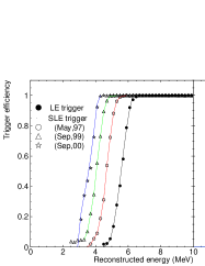
Figure 3: Trigger efficiency as a function of energy. The left plot shows the efficiency as a function of reconstructed energy (see Section IV.3 for the details of reconstructed energy). The May 1997 LE triggers (black circles with black line) and SLE triggers (white circles with red line) were calculated using a Ni(n,$\gamma$)Ni gamma source, while the SLE triggers on September 1999 (triangles with green line) and September 2000 (stars with blue line) were calculated using ¹⁶N events from a DT generator. The right plot shows the efficiency as a function of true electron total energy obtained by a Monte Carlo simulation. Identically colored lines represent the same calibration data samples in both plots.

III Simulation

In the simulation of solar neutrino events in Super–Kamiokande–I there are several steps: generate solar neutrinos, determine recoil electron kinematics, generate and track Cherenkov light in water, and simulate response of electronics.

In order to generate the ⁸B solar neutrino spectrum in Monte Carlo, the calculated spectrum based on the ⁸B decay measurement of Ortiz et al. ortiz was used. Figure 4(a) shows the input solar neutrino energy distribution for ⁸B neutrinos. For the uncertainty in the spectrum we have adopted the estimation by Bahcall et al bpspc .

In the next step, the recoil electron energy from the following reaction;

$$\nu+e\to\nu+e$$ (1)

is calculated. Fig 4(b) shows the differential cross section. The $(\nu_{e},e)$ scattering cross section is approximately six times larger than $(\nu_{\mu,\tau},e)$, because the scattering of $\nu_{e}$ on an electron can take place through both charged and neutral current interactions, while in case of $\nu_{\mu,\tau}$ only neutral current interactions take place. The radiative corrections in the scattering are also considered rad . Figure 4(c) shows the expected spectrum of recoil electrons in SK without neutrino oscillations.

Assuming the ⁸B flux of BP2004 ($5.79\times 10^{6}/cm^{2}/sec$) and before taking into account the detector’s trigger requirements, the expected number of $\nu_{e}$ scatter events in SK is 325.6 events per day. MC events are generated assuming a rate of 10 recoil electron events per minute for the full operation time of SK–I, yielding a total of 24,273,070 simulated solar neutrino events.

Figure 4: (a) Input distributions of ⁸B (solid) and hep (dashed) solar neutrino energies. (b) The cross section of the interaction for $\nu_{e}$ (solid line) and $\nu_{\mu,\tau}$ (dashed line) with electrons as a function of neutrino energy. (c) The spectrum of recoil electrons scattered by ⁸B and hep solar neutrinos.

We have used GEANT3.21 for simulation of particle tracking through the detector. Since the tracking of Cherenkov light is especially important in the Super–K detector, parameters related to photon tracking are fine tuned through the use of several calibration sources.

Figure 5 shows the wavelength dependence of various water coefficients in our MC. Rayleigh scattering is dominant at short wavelengths with a 1/$\lambda^{4}$ dependence. The $\lambda$ dependence of absorption and Mie scattering are empirically set to 1/$\lambda^{4}$ at shorter wavelengths, while the absorption for longer wavelengths are taken from a separate study water . The absorption and scattering coefficients in MC are tuned using LINAC calibration data (see Section V.2.1) so as to match the MC and data energy scale in each position in the detector.

The water quality in SK changes as a function of time as shown in Figure 17; this change in water quality was taken into account in the MC simulation. By comparing photon arrival timing distributions using calibration data, it was found that the change in water attenuation length is mainly due to change in the absorption coefficient. So, we fixed Rayleigh scattering and Mie scattering coefficients to be constant over the entire data taking period and vary only the absorption coefficient in the MC simulation. Figure 6 shows the result. The solid line shows the translation of water transparency into the absorption coefficient. The lower panel shows the deviation of the peak of the reconstructed energy from the peak of the input energy as a function of water transparency — the deviation is less than $\pm 0.2\%$. The coefficients of each process at shorter wavelength are summarized as follows:

$$8.00\times 10^{7}/\lambda^{4}[nm]\quad(1/m) :$$ Rayleigh scat.,

$$1.00\times 10^{8}/\lambda^{4}[nm]\quad(1/m) :$$ Mie scat.,

$$(2.74\sim 9.27)\times 10^{7}/\lambda^{4}[nm]\quad(1/m) :$$ absorption.

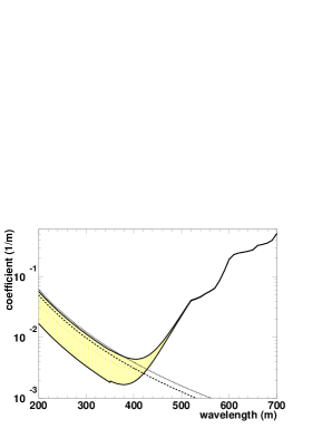
Figure 5: Wavelength dependence of the water parameter coefficients: absorption (solid), Rayleigh scattering (dashed) and Mie scattering (dotted). The absorption coefficient is also a function of water transparency. The filled region shows the range of this parameter as water transparency is changed, where the two solid lines define the SK–I minimum (73 meter) and maximum (98 meter) values.

Figure 6: Translation of the water transparency parameter into a short wavelength absorption coefficient. Absorption is taken to be proportional to $\lambda^{-4}$ for these wavelengths. Light scattering is assumed to be constant. The lower panel shows the energy deviation as a function of input momentum. The inner error bar of each point is the statistical uncertainty, while the outer error bar represents the spread of the six samples using 5, 6, 8, 10, 12, and 15 MeV/c as the input momenta.

IV Event reconstruction method

IV.1 Vertex

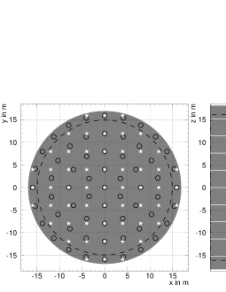
Figure 7: Search grid for the vertex reconstruction in the $xy$ plane and in $z$. The shaded area is the SK inner detector volume. The dashed line indicates the fiducial volume. The white stars (white lines) are the grid points used by the standard vertex reconstruction. The black circles are used by the second vertex reconstruction.

Electrons in the energy region of interest for solar neutrinos (below 20 MeV) can travel only a few centimeters in water, so their Cherenkov light is approximately a point source. The reconstruction of this vertex relies solely on the relative timing of the “hits,” i.e., PMT’s struck by one or more Cherenkov photons. Since the number of observed Cherenkov photons and therefore the likelihood of a multiply hit PMT is comparatively small, about seven recorded photons per MeV of deposited energy, the pulse heights of the hits typically follows a one photo-electron distribution and yields no information about the light intensity nor the distance to the source. For the same reason it is also impossible to separate reflected or scattered Cherenkov photons and PMT dark noise from direct light based upon PMT pulse height. The vertex reconstruction assumes that a photon originating from vertex $\vec{v}$ and ending in hit $\vec{h}_{i}$ is traveling on a straight path and therefore takes the time $|\vec{v}-\vec{h}_{i}|/c$ where c is the group velocity of light in water (about 21.6 cm/ns). Therefore, assuming only direct light, the effective hit times $\tau_{i}=t_{i}-|\vec{v}-\vec{h}_{i}|/c$ at vertex $\vec{v}$ of all PMT’s should peak around the time of the event with the width of the PMT timing resolution for single photoelectrons (about 3 ns). Light scattering and reflection (as well as dark noise, pre-, and afterpulsing of the PMT’s) introduces tails in the distribution which will strongly bias the reconstruction if a $\chi^{2}$ is used to evaluate the goodness of fit $g$ for a given vertex. Therefore, we use a “truncated $\chi^{2}$”

$$g(\vec{v})=\sum_{i=1}^{N}e^{-\frac{1}{2}\left(\frac{\tau_{i}-t_{0}}{\sigma_{t}}\right)^{2}}$$ (2)

where $t_{0}$ is the center of a 10 ns wide search window in $\tau$ which maximizes the number of hits inside. The vertex is reconstructed by the maximization of this goodness varying $\vec{v}$.

We use three different vertex reconstruction algorithms. Our standard vertex fit is used to reconstruct event direction and energy and to compute the likelihood of an event to be due to spallation. Only events inside the fiducial volume (2 m away from the closest PMT) are considered. The Super–K background rate below about 7 MeV rises rapidly with falling energy; most of this background is due to light emanating from or near the PMT’s themselves and is reconstructed outside the fiducial volume. However, the rate of misreconstructed events (background events outside the fiducial volume which get reconstructed inside) increases rapidly with falling energy due to long resolution tails. We therefore reconstruct the vertex using a second vertex fitter whose vertex distribution has smaller tails and then accept only events reconstructed inside the fiducial volume by both fits. To reduce the rate of SK events stored to tape, we remove SLE events which reconstruct outside of the fiducial volume online. Unfortunately, both offline fitters are too slow to keep up with the trigger rate (see Section 3) of SLE events and so we are forced to use a fast reconstruction to pre-filter these events. If the vertex of the fast online fit is inside the fiducial volume the event is reconstructed later by the other two fits.

To ensure convergence of the maximum search, the standard fit first evaluates the vertex goodness on a Cartesian grid (see Figure 7). For a reasonably speedy search in spite of Super–Kamiokande’s large size, a coarse grid of 57 points with a grid constant of 397.5cm is chosen for the $xy$ plane with nine such layers in $z$ separated by 380 cm. Since the grid is coarse, the timing resolution $\sigma_{t}$ is artificially set to 10 ns to smear out the maximum goodness. After the single coarse grid point with the largest goodness is identified, the goodness is calculated at the 27 points of a $3\times 3\times 3$ cube centered on this grid point with a timing resolution of $\sigma_{t}=5$ ns and a spatial grid separation of 156 cm. If the largest resulting goodness is not in the center, the cube is shifted so that the largest goodness is in the center of the new cube. Otherwise, the cube is contracted by a factor of 2.7. If the spatial grid separation of the cube reaches 5 cm the maximum search is finished and the reconstructed vertex is the point with the largest found goodness.

To limit the bias of the vertex reconstruction due to the tails in the timing residuals $\tau_{i}-t_{0}$, the hits that go in the vertex fit are selected. Since the event vertex is not known, the hit selection must be based on the absolute hit times $t_{i}$ (and the spatial distribution of the hits $\vec{h}_{i}$). The hit selection of the standard reconstruction first finds the start time of a sliding 200 ns window (the time required for a photon to cross the diagonal of the detector) which contains the largest number of hits. The rate of late/early hits (background) per ns is determined by counting the hits outside the window. From this rate, the background inside the window is estimated. The size of the window is then reduced in an attempt to optimize the direct light signal divided by the square root of the late/early hit background. The hits in the resulting, optimal timing window are those selected to compute the vertex goodness.

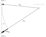
Figure 8: Timing constraint for pairs of hits. From the triangle relation $ct_{i}+\Delta x>ct_{j}=ct_{i}+\Delta ct_{ij}$ follows $\Delta t_{ij}<\Delta x/c=|\vec{h}_{i}-\vec{h}_{j}|/c$.

The second vertex reconstruction (to reduce misreconstructed events originating from the PMT’s) modifies the hit selection and the search grid. For two direct light hits $i$ and $j$, the timing difference $\Delta t_{ij}$ is limited to $\Delta t_{ij}<|\vec{h}_{i}-\vec{h}_{j}|/c$ (see Figure 8). We select the largest set of hits whose hit pairs obey $\Delta t_{ij}<|\vec{h}_{i}-\vec{h}_{j}|/c$ after eliminating “isolated hits” (hits which are further away than 1250 cm or further away than 35 ns from the nearest neighboring hit). With these selected hits we perform a grid search with a circular grid of 60 points on the $xy$ plane (grid constant 397.5 cm) and nine such planes in $z$ separated by 380 cm with a timing resolution of 9.35 ns. The best fit point is interpolated from the grid points with the largest goodness. After that, 27 points of a cylindrical section around that point with an initial grid constant of 147.1 cm and 5 ns resolution are tested. As in the standard reconstruction, the section is moved (if the center point doesn’t have the largest goodness) or reduced in size by a factor of 0.37 (if it does), and the search is finished once the grid constant falls below 5 cm.

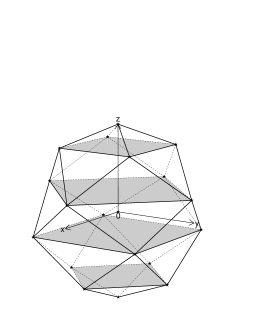
Figure 9: Search grid for the fast fit. 18 points around the input vertex are tested, the orientation is fixed. The grid size is adjusted between one and eight meters (see Table 2).

Step Size [cm] $t_{0}\pm\sigma_{t}$ [ns] $a_{0}\pm\sigma_{a}$ $t_{\mbox{\tiny win}}$ [ns] 1 800 $2.1\pm 10.2$ $0.534\pm 0.134$ (-66.7,100.0) 1 $2.7\pm 6.1$ $0.534\pm 0.134$ (-40.0, 66.7) 2 400 $2.3\pm 6.0$ $0.534\pm 0.134$ (-33.3, 50.0) 3-5 $2.3\pm 6.0$ $0.534\pm 0.134$ (-25.0, 33.3) 1 $1.5\pm 4.7$ $0.1g$ for $a<0.2,a\geq 0.9$ (-20.0,33.3) 2 200 $2.2\pm 4.5$ $g$ for $0.3\leq a<0.85$ (-20.0,33.3) 3-5 $1.1\pm 4.1$ $0.5g$ otherwise (-20.0,26.7) 1-8 100 $0.6\pm 3.2$ none (-13.3,16.7)

Table 2: Search parameters for the fast fit.

The fast fit, used to pre-filter SLE events online, also eliminates isolated hits (i.e., all other hits separated by either more than 10 m or more than 33.3 ns) to reduce the effects of dark noise and reflected or scattered light. Then the absolute peak time is estimated by maximizing the number of PMT hits within a 16.7 ns wide sliding timing window. PMTs that are in the interval ($-33.3$ ns, 100 ns) with respect to the peak time are selected. An initial vertex is calculated by shifting a simple average of the selected PMT positions 2 m toward the detector’s center. The time at the event vertex is also determined; this time must be smaller than the absolute peak time yet not differ from it by more than 117 ns. The initial vertex time is chosen to be 58.3 ns before the absolute peak time. It is then corrected to the average of all time-of-flight subtracted PMT times that are in the interval ($-133.3$ ns, 200 ns) around the initial time. The magnitude of the anisotropy

$$\vec{a}=\frac{\sum_{\mbox{\tiny selected hits}}q_{i}(\vec{h}_{i}-\vec{v})/|\vec{h}_{i}-\vec{v}|}{\sum_{\mbox{\tiny selected hits}}q_{i}}$$ (3)

is also calculated at this stage. Next, 18 points around the initial vertex are tested with an initial search radius of 8 m (see Table 9), while the goodness $g$ is modified to take into account the anisotropy. At first, the goodness is multiplied by the factor $e^{-0.5((a-a_{0})/\sigma_{a})^{2}}$. Later in the search, this factor is replaced by a table. The times are shifted by the expected mismatch between the average vertex time and the vertex peak time $t_{0}$. Only hits inside a time interval around the shifted vertex time are considered. The search radii, time shifts, time resolutions, anisotropy factors, and time intervals are listed in Table 2.

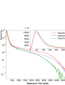
Figure 10: Distance from reconstructed to correct vertex for ⁸B Monte Carlo events with total recoil electron energy above 4.5 MeV. The inserted panel magnifies the distributions near zero on a linear scale.

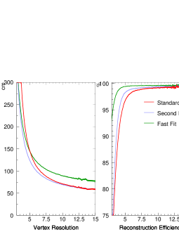
Figure 11: Vertex resolution (68.2% of reconstructed events reconstruct inside a sphere of radius $\sigma$ from correct vertex) of ⁸B Monte Carlo events as a function of total recoil electron energy. The curves on the right-hand side show the fraction of reconstructed events as a function of total recoil electron energy.

As shown in Figures 10 and 11, the performance of all three fitters is evaluated using ⁸B Monte Carlo. The distribution of the distance between the reconstructed and correct vertex is analyzed for each fit (see Figure 10); the vertex resolution is extracted as the distance which contains 68.2% of all reconstructed vertices. For recoil electrons above 4.5 MeV, the fast fit shows the worst resolution (115 cm). However, it has the lowest rate of very distant misfits ($>30$ m). The resolution of the standard fit is 102 cm, while the second fit’s resolution is 94 cm. Figure 11 shows the vertex resolution as a function of generated total recoil electron energy. Since the vertex reconstruction occasionally fails (due to a number of selected hits that is too small), the efficiency to reconstruct the event anywhere at all is also plotted.

IV.2 Direction

Since the recoil electron preserves the direction of the solar neutrino, directional reconstruction is important for solar neutrino analysis. This characteristic directionality is used to extract the solar neutrino signal in Super–K. To calculate the direction, a maximum likelihood method using the Cherenkov ring pattern is adopted. The likelihood function is

$$L(\vec{d})\equiv\sum_{i}^{N_{30}}\log(f{(\cos\theta_{dir})})_{i}\times\frac{\cos\theta_{i}}{a(\theta_{i})}.$$ (4)

where $N_{30}$ is the number of hit PMT’s with residual times within a 30 nsec window and $f{(\cos\theta_{dir})}$ is the function that represents the distribution of the opening angle between the particle direction and the vector from the reconstructed vertex to the hit PMT position made by MC. A plot of $f{(\cos\theta_{dir})}$ for 10 MeV electrons is shown in Figure 12. The distribution is broad with the peak at $42^{\circ}$ because of the effects of electron multiple scattering and Cherenkov light scattering in water. $\theta_{i}$ is the opening angle between the direction of the vector from the reconstructed vertex to the i-th hit PMT position and the direction that PMT is facing. $a(\theta_{i})$ is the acceptance of PMT’s as a function of $\theta_{i}$ which is made by MC. The direction is reconstructed as Eq. (4) becomes maximum using a grid search method whose step sizes are $20^{\circ},9^{\circ},4^{\circ},1.6^{\circ}$.

Figure 12: The distribution of the opening angle between the direction of the generated particle and the vector from the reconstructed vertex to the hit PMT position. This plot is made for 10 MeV electron MC events.

The quality of the directional reconstruction is estimated from the differences between the generated and reconstructed directions using MC. Figure 13 shows the directional resolution dependence on energy within the fiducial volume; it uses directions which are generated uniformly. Here, the resolution is defined as the 68% point for the angle difference distribution. The angular resolution for 10 MeV electrons is about 25 degrees.

Figure 13: The directional resolution’s dependence on energy, determined using Monte Carlo events.

IV.3 Energy

The energy of a fully-contained charged particle in Super–Kamiokande is approximately proportional to the number of generated Cherenkov photons, and thus is also proportional to the total number of photo-electrons in the resulting hit PMT’s. When the particle’s energy is low it is also proportional to number of hit PMT’s because in such a case the number of Cherenkov photons collected by any given PMT is almost always zero or one. In order to avoid the effect of noise hits with higher charge, the number of hit PMT’s $(N_{hit})$ with some corrections is used for energy determination for the solar neutrino analysis. In order to reject accidental hits due to dark noise in the PMT’s, only the hit PMT’s with residual times within a 50 nsec window are used for calculating $N_{hit}$. Moreover, we applied several corrections to $N_{hit}$, yielding an effective number of hits ($N_{eff}$) which has the same value at every position in the detector for a given particle energy. These corrections account for the variation of the water transparency, the geometric acceptance of each hit PMT, the number of bad PMT’s, the PMT dark noise rate, and so on. The equation for $N_{eff}$ is:

$$N_{eff} = \sum_{i=1}^{N_{hit}}\{\left(X_{i}+\epsilon_{tail}-\epsilon_{dark}\right)\times\frac{N_{all}}{N_{normal}}\times$$ (5)

$$\frac{R_{\mbox{cover}}}{S(\theta_{i},\phi_{i})}\times\exp\left(\frac{r_{i}}{\lambda(\mbox{run})}\right)\times G_{i}(t)\}$$

where $X_{i}$ is an occupancy used to estimate the effect of multiple photo-electrons, $\epsilon_{tail}$ is the correction for late hits outside the 50 ns window, and $\epsilon_{dark}$ is for dark noise correction. The definition of $X_{i}$ is as follows:

$$X_{i}=\left\{\begin{array}[]{ll}\displaystyle{\frac{\log\frac{1}{1-x_{i}}}{x_{i}}}&\qquad x_{i}<1\\[14.22636pt] 3&\qquad x_{i}=1\end{array}\right.$$ (6)

where $x_{i}$ is the ratio of the number of hit PMT’s to the total number of PMT’s in a $3\times 3$ patch around the i-th hit PMT. This correction estimates the number of photons which arrived at the i-th hit PMT by using the number of hit PMT’s surrounding it. Here, the ratio of the unhit PMT’s in this patch of nine tubes is $1-x_{i}$.

The second factor is the bad PMT correction, where $N_{all}$ is the total number of PMT’s, 11146, and $N_{normal}$ is the number of properly operating PMT’s for the relevant subrun.

The third factor is the effective photo coverage. The average of the photo coverage, which is the ratio of the area covered by PMT’s to all inner detector area, is $R_{\mbox{cover}}=0.4041$ . However, the effective photo coverage changes with the incident angle of the photon to the PMT. Therefore, we applied a coverage correction, where $S(\theta_{i},\phi_{i})$ is the photo coverage from the directional vantage point of $\theta_{i},\phi_{i}$. Figure 14 shows this function.

The fourth factor is the water transparency correction, where $r_{i}$ is the distance from the reconstructed vertex to the i-th hit PMT position, and $\lambda$ is water transparency.

The fifth factor, $G(t)_{i}$, is the gain correction at the single photo-electron level as a function of the time of the manufacture of each PMT.

Figure 14: Function of the effective photo-coverage’s dependence on the incident angle to a PMT.

Finally, the conversion function from $N_{eff}$ to energy is determined by uniformly generated Monte Carlo vertices. This is total energy; all mention of “energy” hereafter refers to total energy, i.e. including the scattered electron’s rest mass and momentum. The relation to energy is calculated by the following equation;

$$\mbox{E}=\alpha+\beta N_{eff}(1-\gamma N_{eff}(1-\delta N_{eff}(1-\epsilon N_{eff}))),$$ (7)

here $\alpha=0.735,\beta=0.134,\gamma=6.049\times 10^{-4},\delta=6.441\times 10^{-3},$ and $\epsilon=1.541\times 10^{-3}.$ The typical conversion factor from $N_{eff}$ to energy is 6.97. The energy resolution is also estimated by the same MC described above. Figure 15 shows the energy resolution as a function of energy; it is 14.2% for 10 MeV electrons.

Figure 15: The energy resolution’s dependence on energy as determined using Monte Carlo events.

IV.4 Muon

Precise reconstruction of cosmic ray muon tracks which penetrate the Super–K detector is needed for the solar neutrino analysis. This is because nuclear spallation events induced by these cosmic ray muons are a dominant background to the solar neutrino signal, and the correlation in time and space between spallation events and their parent muons is extremely useful in rejecting the spallation background. Hence, the track position precision requirement for our muon fitter is about 70 cm since the vertex resolution for low energy events with energies around 10 MeV is also about 70 cm.

The muon fitter has three components; an “initial fitter,” a “TDC fitter,” and a “geometric check.”

The initial fitter assumes the position of the first fired PMT is the entrance point of a cosmic ray muon, and the center of gravity of the saturated tubes’ positions as the exit point. The PMT at the exit point has the most photo-electrons [p.e.’s] of all PMT’s; the expected value is up to 500 $p.e.$. However, our front end electronics saturate at $\sim 230$ p.e. in a single tube, and so typically several dozen PMT’s near the exit point are saturated. Therefore, the reconstructed exit point is not the position of the most-hit PMT, but rather the center of gravity of the saturated tubes’ positions.

For the entrance position search, we consider the dark noise of the PMT’s. For SK–I the dark noise rate of a typical PMT was $\sim$ 3.5 kHz, though it could rise to $>10$ kHz in the case of a “noisy PMT.” In the initial fitter, the following methods are used to reject dark noise hits:

1. Charge information of PMT
   The fitter requires that the PMT at the entrance point have more than 2 $p.e.$, because typical dark hit PMT’s have less than 1 $p.e.$ while the amount of charge which they receive from a muon is several $p.e.$’s.

2. Timing information of eight neighbor PMT’s
   Cosmic ray muons emit lots of Cherenkov light ($\sim 340$ photons/cm), so several PMT’s near the entrance point should record photons at the same time. The fitter therefore requires that the PMT at the entrance point have more than five fired neighbor PMT’s within 5 ns.

The results of the “initial fitter” are then used as initial values by the next stage.

The TDC fitter is a fitter based on a grid search method using timing information. In this fitter, a goodness of fit is also defined to obtain the best track of the muon:

$$g(\vec{v})=\sum_{i=1}^{N}e^{-\frac{1}{2}\left(\frac{\tau_{i}-t_{0}}{f\times\sigma_{t}}\right)^{2}},$$ (8)

where the definitions are the same as for the “truncated $\chi^{2}$” in Section IV.1 except for the factor ($f$), which is found to be 1.5 by Monte Carlo. The TDC fitter surveys a circle of radius 5.5 m from the exit point obtained by initial fitter and then obtains the direction which maximizes the goodness.

The muon fitter determines the muon track by using two independent parameters, timing and charge, and the two results are sometimes different. For example, in the case of muon bundle events, PMT’s near the exit point fire at early times, because the velocity of a cosmic ray muon is faster than that of light in water. As a result of these early hits, the exit point can sometimes be mistaken for an entrance point. In order to reject this kind of misfit, the geometric check fitter estimates the consistency of both previous fitters by requiring the following after the TDC fit:

• There is no saturated PMT within 3 m from the entrance point.

• There should be some saturated PMT within 3 m from the exit point.

The muon events which do not satisfy these requirements are regarded as failed reconstructions.

We estimated the performance of the muon fitter by using Monte Carlo events. Figure 16 shows the vertex and angular resolutions. For the entrance point, the 1-$\sigma$ vertex resolution is estimated to be 68 cm. This value corresponds closely to the spacing interval between each PMT, 70.7 cm. The vertex resolution of exit point is 40 cm, Therefore, the distance between the actual muon track and the fitted one is estimated to be less than 70 cm, which means that this muon fitter satisfies our precision requirement. The angular resolution is estimated to be 1.6^∘.

Figure 16: Performance of the muon fitter. Left (right) figure shows the vertex (angular) correlation between generated and reconstructed Monte Carlo muon tracks. The area to the left of the dashed line in both plots shows the 1-$\sigma$ (= 68%) included region.

V Calibration

V.1 Water transparancy measurement

Cherenkov photons can travel up to 60 m before reaching PMT’s in Super–K, and so light attenuation and scattering in water directly affects the number of photons that are detected by the PMT’s. Since the energy of an event is mainly determined from the number of hit PMT’s, the water transparency [WT] must be precisely determined for an accurate energy measurement.

The water transparency in SK is monitored continuously by using the decay electrons (and positrons) from cosmic ray $\mu$ events that stop in the detector: $\mu^{-}\to e^{-}+\bar{\nu}_{e}+\nu_{\mu},$ and $\mu^{+}\to e^{+}+\nu_{e}+\bar{\nu}_{\mu}.$ At SK’s underground depth (2700 m.w.e.), cosmic ray muons reach the detector at a rate of $\sim$ 2 Hz. Approximately 6000 $\mu$’s per day stop in the inner detector and produce a decay electron (or positron). In order to monitor the WT effectively, it is important to have a pure sample of $\mu$-e decay events. Several criteria are applied to select these events:

• The time difference [$\Delta T$] between the stopping $\mu$ event and the $\mu$-e decay candidate must satisfy: 2.0 $\mu$sec $<\Delta T<$ 8.0 $\mu$sec.

• The reconstructed vertex of the $\mu$-e decay candidate must be contained within the 22.5 kton fiducial volume.

• $N_{hit}$ must be at least 50.

These criteria select $\sim$1500 $\mu$-e decay events daily, which is sufficient statistics to search for variation in the WT in one week. The average energy of the $\mu$-e decay events is $\sim$ 37 MeV, which is much higher than that of solar neutrinos ($<$ 20 MeV). Therefore, the $\mu$-e decays cannot be used for the absolute energy calibration. However, they can be used to monitor the stability of water transparency and energy scale over time.

In order to remove the effects of scattered and reflected light, hit PMT’s are selected by the following criteria: (1) PMT’s must have timing that falls within the 50 nsec timing window, after the time-of-flight [TOF] subtraction, (2) PMT’s must be within a cone of opening angle $\rm 32^{\circ}\sim 52^{\circ}$ with respect to the direction of the $\mu$-e decay event. A plot of the number of hit PMT’s vs. distance from the vertex to the PMT is made using the selected PMT’s, fit with a linear function, and the inverse of the slope gives the water transparency.

Figure 17(a) shows variations in the WT as a function of time. Each point on the plot represents WT for one week. In order to reduce the effects of statistical fluctuations on the weekly measurement, the WT for a given week is defined as a running average over five weeks of data. Figure 17(b) plots the mean $N_{eff}$ value for $\mu$-e decay events in SK–I. From this figure, it can be seen that the energy scale has remained stable to within $\pm$ 0.5% during the SK–I runtime.

Figure 17: (a) Time variation of the measured water transparency during SK–I. Stability of the SK–I energy scale as a function of time. (b) Each point represents the mean $N_{e}ff$ value for 28 days of $\mu$-e data. The solid line represents the average $N_{e}ff$ for all $\mu$-e events in SK–I; the dashed and dotted lined represent, respectively, $\pm$ 0.5% and $\pm$ 1.0% deviations from the average.

V.2 Energy calibration

The energy scale calibration is necessary to correctly convert the effective number of hits ($N_{eff}$) to the total energy of the recoil electrons induced by solar neutrinos. LINAC and DT calibration are discussed in this section.

V.2.1 LINAC

The primary instrument for energy calibration is an electron linear accelerator [LINAC]. The LINAC calibration of Super–K has been discussed in detail elsewhere linac . The LINAC is used to inject downward-going electrons of known energy and position into the SK tank. The momentum of these electrons is tunable, with a range of 5.08 MeV to 16.31 MeV; this corresponds well with the energies of interest to solar neutrino studies. LINAC data is collected at nine different positions in the SK tank, as shown in Figure 18. The data are compared to MC, and MC is adjusted until its absolute energy scale agrees well with data in all the positions and momenta. Once adjusted, this MC is extrapolated to cover events in all directions throughout the entire detector.

The electrons are introduced into SK via a beam pipe whose endcap’s exit window is a 100 $\mu$m-thick sheet of titanium. This allows electrons to pass through without significant momentum loss but prevents water from entering the beam pipe.

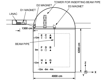
Figure 18: The LINAC system at SK. The dotted line represents the fiducial volume of the detector and the black dots indicate the positions where LINAC data were taken.

Seven different momentum data sets are taken at each LINAC position. The absolute energy in the LINAC system is measured with a germanium [Ge] detector. Table 3 shows the different momenta used in the LINAC calibration. The average occupancy at the beam pipe endcap is set to about 0.1 electrons/spill. The reason for this low occupancy is to reduce the number of spills which include multiple electrons.

beam momentum	Ge energy	in-tank energy
(MeV/c)	(MeV)	(MeV)
5.08	4.25	4.89
6.03	5.21	5.84
7.00	6.17	6.79
8.86	8.03	8.67
10.99	10.14	10.78
13.65	12.80	13.44
16.31	15.44	16.09

Table 3: LINAC beam momentum. The second column gives the energy measured in the Ge calibration system. The last column lists the total energy of the electrons after leaving the beam pipe.

The energy scale and resolution obtained by LINAC is compared to MC at each position and momentum. Figure 19(a) shows the deviation in the energy scale between data and MC. Figure 19(b) shows the average over all the positions from (a). The deviation at each position is less than 1% and the position averaged momentum dependence of the deviation is less than 0.5%.

Figure 19: The relative difference between the reconstructed energy of LINAC data and the corresponding MC. (a) The results are shown for all positions and beam momenta. (b) Averaged over all positions. The dashed lines show $\pm$ 0.5%. See Fig. 18 for the positions.

Figure 20 (a) shows the deviation of the energy resolution at each energy and position in LINAC calibration between data and MC, and (b) shows these deviations averaged over all positions. The difference in reconstructed energy resolution between data and MC is less than 2.5%.

Figure 20: The reconstructed energy resolution from LINAC data and MC. (a) shows the deviation of the resolution in each energy and position in LINAC calibration between data and MC. (b) Averaged over all positions. The dashed lines show $\pm$ 2.5%. See Fig. 18 for the positions.

The absolute energy scale of the detector was tuned by using the LINAC calibration data. The uncertainty of the absolute energy scale comes from the uncertainties of water transparency measurement when the LINAC calibration data was taken (0.22%), position dependence of the energy scale (0.21%), time variation of the energy scale obtained by LINAC calibration (0.11%), tuning accuracy of MC simulation (0.1%), electron beam energy determination in LINAC calibration (0.21%), and directional dependence of energy scale since the LINAC beam is only downward-going (0.5%). Adding those contributions in quadrature, the total uncertainty of Super–K–I’s absolute energy scale is estimated to be 0.64%.

V.2.2 ${}^{16}N$ from the DT Generator

Even though the energy scale is determined from LINAC calibration and is fixed, ${}^{16}N$ was also used as a calibration source. Since events from ${}^{16}N$ decay are isotropic, they are useful in probing the directional dependence of the energy scale. Also, because of the portability of the DT generator we were able to probe the energy scale at many positions in the detector on a monthly basis.

With a half-life of 7.13 seconds, the Q-value of the decay of ${}^{16}N$ is 10.4 MeV, and the most probable decay mode produces a 6.1 MeV $\gamma$ ray together with a $\beta$ decay electron of maximum energy 4.3 MeV. Man-made ${}^{16}N$ was obtained using a deuterium-tritium neutron generator [“DT generator”]. The DT generator uses the fusion reaction ${}^{2}H+^{3}H\rightarrow^{4}He+n$ to produced 14.2 MeV neutrons. A fraction of the neutrons collide with ${}^{16}O$ to produce ${}^{16}N$. The DT generator thus provided us with a large sample of essentially background free ${}^{16}N$ data for use in energy scale calibration. More details about the DT generator are given elsewhere nim_dt .

The ${}^{16}N$ decay energy spectrum is a superposition of several $\gamma$ ray lines and $\beta$ continua of various end points. The reconstructed energy spectrum has a peak around $\mbox{$E_{peak}$}=6.9\sim 7.0$ MeV. The shape of the peak region ($5.5\sim 9.0$ MeV) is approximated by a Gaussian with a width of $1.6\sim 1.7$ MeV. The deviation of this energy peak between data and MC is measured. Figure 21 shows 31 data sets of DT results during two years of running, and it shows the deviation is within $\pm 1\%$ when averaged over all positions.

Figure 21: The deviation between data and MC for the volume-averaged DT energy scale as a function of time. The DT generator was available for the last two years of SK–I, starting in July, 1999. The dashed line shows the $\pm$0.64% of energy scale uncertainty, which is estimated by LINAC calibration as discussed in SectionV.2.1.

The direction dependence of the energy scale is measured as follows. First, the deviation between data and MC is calculated for all directions. Then it is calculated for two divided data samples: events in the upward or downward directions. It should be noted that in all cases, the energy scale is averaged over the detector volume. Figure 22 shows plots comparing the energy scale obtained from using just downward- or upward-going events to that determined by using the entire sample. The difference is within $\pm 0.6\%$.

Figure 22: Directional dependence of energy scale by DT calibration. Upper figure shows $\mbox{$R_{down}$}-R$ as a function of time, lower figure shows the same for $\mbox{$R_{up}$}-R$. Note that $\mbox{$R_{up}$}\approx-\mbox{$R_{down}$}$.

V.3 Vertex calibration

Figure 23 shows the vertex resolution in each energy and position in LINAC and Monte Carlo. The differences of vertex resolution between data and MC is less than $\pm 5$ cm.

The vertex shift in the reconstruction is estimated using a Ni(n,$\gamma$)Ni gamma source, sk_detector because the gamma ray is emitted in almost uniform directions. The vertex shift is defined as a vector from an averaged position of the reconstructed vertex of the data to that of a corresponding MC. Table 4 shows the vertex shift at several source positions. The systematic error for the solar neutrino flux as a result of vertex shift (which could move events in or out of the fiducial volume) is evaluated from these values, and it is $\pm 1.3\%$.

Figure 23: The reconstructed vertex resolution from LINAC data and MC. (a) shows the deviation of the resolution in each energy and position in LINAC calibration between data and MC. (b) averaged over all positions. The dashed lines show $\pm$ 5 cm. See Fig. 18 for the positions.

Position	$\Delta x$	$\Delta y$	$\Delta z$
(35.3,-70.7,-1200)	-1.8	-1.9	-2.8
(35.3,-70.7,0)	0.6	-0.5	-2.8
(35.3,-70.7,+1200)	-1.1	-1.7	0.6
(35.3,-70.7,+1600)	0.0	-3.2	-3.5
(35.3,-1555.4,-1200)	-5.5	8.6	-9.1
(35.3,-1555.4,0)	-5.5	23.4	-3.0
(35.3,-1555.4,+1200)	-0.5	7.0	6.0
(35.3,-1555.4,+1600)	-3.3	7.6	2.7
(35.3,-1201.9,-1200)	-4.2	5.4	-9.1
(35.3,-1201.9,0)	-1.4	15.5	-2.2
(35.3,-1201.9,+1200)	2.5	8.9	4.2
(1520.0,-70.9,-1200)	-5.7	-1.4	-10.3
(1520.0,-70.9,0)	-18.6	-3.0	-4.0
(1520.0,-70.9,+1200)	-12.6	-1.0	6.2
(-35.3,-1555.4,-1200)	3.7	-11.4	-8.6
(-35.3,-1555.4,0)	6.6	-19.5	-2.0
(-35.3,-1555.4,+1200)	1.6	-20.3	7.2

Table 4: The vertex shift measured by Ni(n,$\gamma$)Ni gamma source calibration. The unit is cm.

V.4 Direction calibration

The angular resolution is calibrated by LINAC data and MC. Figure 24 shows the angular resolution variation in each energy and position between LINAC and Monte Carlo events. The difference in angular resolution between LINAC data and MC is less than $\pm 0.5$ degree.

We have applied this difference as a correction factor to the expected signal shape, then taken the same amount of the correction as our systematic error due to angular resolution. This systematic error is 1.2%.

Figure 24: The reconstructed angular resolution from LINAC data and MC. (a) shows the deviation of the resolution in each energy and position in LINAC calibration between data and MC. (b) is averaged over all positions. The dashed lines show $\pm$ 0.5 degree. See Fig. 18 for the positions.

VI Background

VI.1 Low energy backgrounds

The main background sources below about 6.5 MeV for the solar neutrino events are (1) events coming from outside fiducial volume, and (2) ²²²Rn.

Figure 25 shows a typical vertex distribution of the low energy events before the Intelligent Trigger selection.

Figure 25: Typical vertex distribution of the low energy events before the Intelligent Trigger selection. The analysis energy threshold for this plot is 5.0 MeV. The dashed line shows the fiducial volume edge.

Most of the low energy events occur near the inner detector’s wall region. They originate from radioactivity of the PMT’s, black sheet, PMT support structures, and mine rocks surrounding the SK detector. Though the fiducial volume is selected to be 2 m from this inner detector wall, there are a lot of remaining events around the edge of the fiducial volume. The reconstructed directions of these remaining, externally-produced events in the fiducial volume are pointed, on average, strongly inward. We have eliminated most of these external events by using an event selection based upon vertex and direction information. The details of this event selection will be explained in Section VII.4. Although most of these external events are eliminated by this cut, some quantity of external events still remain. These remaining external events are one of the major backgrounds in this energy region.

Another major source of background in the low energy region are radioactive daughter particles from the decay of ²²²Rn. ²¹⁴Bi, which is one of these daughter particles, undergoes beta decay with resulting electron energies up to 3.26 MeV. Due to the limited energy resolution of the detector, these electrons can be observed in this energy region.

We have reduced ²²²Rn in the water by our water purification system to contribute less than 1 mBq/m³ sk_detector , and monitor the radon concentration in real-time by several radon detectors radon1 ; radon2 ; radon3 . However, the water flow from the water inlets, located at the bottom of the SK detector, stirs radon emanated from the inner detector wall into the fiducial volume radon4 . Therefore, there is an event excess after the external event cut in the detector bottom region as compared to the top region. We also supply radon-reduced air radon4 into the space above the water surface in the SK tank to prevent radon in the mine air from dissolving into the purified water. The radon concentration in this radon-reduced air is less than 3 mBq/m³ and the measured radon level in the air in the tank is stable at 20$\sim$30 mBq/m³. Periods of anomalously high radon concentration due to water system troubles were removed from this analysis.

VI.2 High energy backgrounds

Above about 6.5 MeV, the dominant background source is radioactive isotopes produced by cosmic ray muons’ spallation process with oxygen nuclei. Some fraction of downward-going cosmic ray muons interact with oxygen nuclei in the water and produce various radioactive isotopes. These radioisotopes are called “spallation products.” Table 5 shows a summary of possible spallation products in SK. The $\beta$ and/or $\gamma$ particles from the radioactive spallation products are observed in Super–K, causing what are called “spallation events.” The spallation events retain some correlation in time and space with their parent muons. Using this correlation, we have developed a cut to remove these spallation background events efficiently. The detail of this cut will be explained in Section VII.2.

Isotope	$\tau_{\frac{1}{2}}$(sec)	Decay mode	Kinetic Energy(MeV)
${}^{8}_{2}$He	0.119	$\beta^{-}$	9.67 + 0.98 ( $\gamma$ )
		$\beta^{-}$ n	( 16 % )
${}^{8}_{3}$Li	0.838	$\beta^{-}$	$\sim$13
${}^{8}_{5}$B	0.77	$\beta^{+}$	$\sim$13.9
${}^{9}_{3}$Li	0.178	$\beta^{-}$	13.6 ( 50.5 % )
		$\beta^{-}$ n	( $\sim$50 % )
${}^{9}_{6}$C	0.127	$\beta^{+}$ p	3 $\sim$ 15
${}^{11}_{3}$Li	0.0085	$\beta^{-}$	16 $\sim$ 20 ($\sim$50%)
		$\beta^{-}$ n	$\sim$16 ($\sim$50%)
${}^{11}_{4}$Be	13.8	$\beta^{-}$	11.51 ( 54.7 % )
			9.41 + 2.1 ( $\gamma$ ) ( 31.4 % )
${}^{12}_{4}$Be	0.0236	$\beta^{-}$	11.71
${}^{12}_{5}$B	0.0202	$\beta^{-}$	13.37
${}^{12}_{7}$N	0.0110	$\beta^{+}$	16.32
${}^{13}_{5}$B	0.0174	$\beta^{-}$	13.44
${}^{13}_{8}$O	0.0086	$\beta^{+}$	13.2, 16.7
${}^{14}_{5}$B	0.0138	$\beta^{-}$	14.55 + 6.09 ( $\gamma$ )
${}^{15}_{6}$C	2.449	$\beta^{-}$	9.77 ( 36.8 % )
			4.47 + 5.30 ( $\gamma$ )
${}^{16}_{6}$C	0.747	$\beta^{-}$ n	$\sim$4
${}^{16}_{7}$N	7.13	$\beta^{-}$	10.42 ( 28.0 % )
			4.29 + 6.13 ( $\gamma$ ) ( 66.2 % )

Table 5: Possible radioactive spallation products in Super–Kamiokande.

VII Data analysis

VII.1 Noise reduction

The first step of the data reduction is an elimination of the noise and obvious background events. First of all, the events with total photoelectrons less than 1000, which corresponds to $\sim 100$ MeV, are selected. Next, the following data reductions are applied: (a) Events whose time difference since a previous event was less than 50 $\mu$sec were removed in order to eliminate decay electrons from stopping muons. (b) Events with an outer detector trigger and over 20 outer PMT hits were removed in order to eliminate entering events like cosmic ray muons. (c) A function to categorize noise events is defined by the ratio of the number of hit PMT’s with $|Q|\leq 1.0$ p.e. and the total number of hit PMT’s. Since typical noise events should have many hits with low charge, events with this ratio larger than 0.4 were removed. (d) A function which can recognize an event where most of its hits are clustered in one electronics module [ATM] is defined. It is the ratio of the maximum number of hits in any one module to the total number of channels (usually 12) in one ATM module. Events with a larger ratio than 0.95 were removed as they generally arose due to local RF noise in one ATM module. (e) Events produced by flasher PMT’s must be removed. These flasher events often have a relatively larger charge than normal events, therefore they are recognized using the maximum charge value and the number of hits around the maximum charge PMT. The slightly involved criteria is shown in Figure 26. (f) An additional cut to remove noise and flasher events is applied using a combination of a tighter goodness cut($goodness\leq 0.6$) and a requirement of azimuthal uniformity in the Cherenkov ring pattern. Good events have a uniform azimuth distribution of hit-PMT’s along the reconstructed direction, while flasher events often have clusters of hit PMT which lead to a non-uniform azimuth distribution.

Figure 26: The relation between max charge and the number of hit PMT’s in a $5\times 5$ patch surrounding the PMT with the maximum charge. At most 24 tubes in this patch (plus the one at the center) can be activated. The upper plot shows a typical distribution including active flasher events, and the lower plot shows a typical good data set. The cut region is the area above the line in the upper figure.

In this noise reduction, the number of candidate solar neutrino events went from $3.43\times 10^{7}$ to $1.81\times 10^{7}$ after applying the 2 m fiducial volume cut and constraining the energy region from 5.0 to 20.0 MeV. Table 7 shows the reduction step summary.

The loss of solar neutrino signal by the noise reduction is evaluated to be $0.8\%$ using a Ni(n,$\gamma$)Ni gamma source at several edge positions of the inner detector. The difference between data and MC for this source yields the systematic error for this series of reductions; it’s $\pm 1.0\%$ for our solar neutrino flux measurement. The loss is mainly due to the flasher cut.

VII.2 Spallation cut

The method to reject spallation products shown in Section VI is described in this section. In order to identify spallation events, likelihood functions are defined based on the following parameters:

• $\Delta L$ : Distance from a low energy event to the track of the preceding muon.

• $\Delta T$ : Time difference from muon event to the low energy event.

• $Q_{res}$ : Residual charge of the muon event, $Q_{total}-Q_{unit}\times L_{\mu}$, where $Q_{total}$ is the total charge, $Q_{unit}$ is the total charge per track length and $L_{\mu}$ is reconstructed track length of the muon track.

Some fraction of muons deposit very large amounts of energy in the detector and in such cases vertex position reconstruction is not reliable. Therefore, the spallation likelihood functions are defined for the following two cases,
in the case of a successful muon track fit;

$$L_{spa}(\Delta L,\Delta T,Q_{res})=$$ (9)

$$L_{spa}^{\Delta L}(\Delta L,Q_{res})\times L_{spa}^{\Delta T}(\Delta T)\times L_{spa}^{Q_{res}}(Q_{res}),$$

in the case of a failure fit the muon track;

$$L_{spa}(\Delta T,Q_{total})=L_{spa}^{\Delta T}(\Delta T)\times L_{spa}^{Q_{total}}(Q_{total}).$$ (10)

where $L_{spa}^{\Delta L}(\Delta L,Q_{res})$, $L_{spa}^{\Delta T}(\Delta T)$, $L_{spa}^{Q_{res}}(Q_{res})$ and $L_{spa}^{Q_{total}}(Q_{total})$ are likelihood functions for $\Delta L$, $\Delta T$ and $Q_{res}$.

Figure 27 shows the $\Delta L$ distributions from spallation candidates for six $Q_{res}$ ranges, and the spallation-like function is made from these plots. Here, the selection criteria is $\Delta T<0.1~{}sec$ and $N_{eff}\geq 50$ (equivalent to 7.2 MeV). The peak around 0 $\sim$ 100 cm is caused by spallation events and that around 1500 cm is due to chance coincidence. The distribution of non-spallation events is calculated using a sample which shuffles the event times time randomly; it is the dashed line in the figure, and the non-spallation-like function is also made by these plots. After subtracting the non-spallation from the spallation function, and taking a ratio with a random coincidence distribution, $L_{spa}^{\Delta L}(\Delta L,Q_{res})$ was obtained.

Figure 27: $\Delta L$ distribution for each $Q_{res}$ ranges, (1) $Q_{res}<2.4\times 10^{4}$ p.e. (2) $2.4\times 10^{4}<Q_{res}<4.8\times 10^{4}$ p.e. (3) $4.8\times 10^{4}<Q_{res}<9.7\times 10^{4}$ p.e. (4) $9.7\times 10^{4}<Q_{res}<4.8\times 10^{5}$ p.e. (5) $4.8\times 10^{5}<Q_{res}<9.7\times 10^{5}$ p.e. (6) $9.7\times 10^{5}$ p.e.$<Q_{res}$. The solid line shows the data, and the dashed line shows the random sample.

Figure 28 shows the $\Delta T$ distributions from spallation candidates for each time range. Here, the selection criteria is $\Delta L<$ 300 cm and $N_{eff}\geq 50$ and $Q_{res}<10^{6}$ p.e.. These distributions are fitted with the following function:

$$L_{spa}^{\Delta T}(\Delta T)=\sum_{i=1}^{7}A_{i}\left(\frac{1}{2}\right)^{-\frac{\Delta T}{\tau^{i}_{1/2}}}$$ (11)

where $\tau^{i}_{1/2}$ are half-life times of typical radioactive elements produced by spallation. The evaluated half-life times and radioisotopes are summarized in Table 6.

Figure 28: $\Delta T$ distribution for each time range, (1) $0.0<\Delta T<0.1$ sec (2) $0.1<\Delta T<0.8$ sec (3) $0.8<\Delta T<4.0$ sec (4) $4.0<\Delta T<15$ sec (5) $15<\Delta T<100$ sec (6) $0<\Delta T<100$ sec. Cross marks are data and lines are fitted likelihood function $L_{spa}^{\Delta T}(\Delta T)$

.

$i$	radioactivity	$\tau^{i}_{1/2}$	$A_{i}$
1	${}^{12}_{5}$B	$2.02\times 10^{-2}$	$1.20\times 10^{5}$
2	${}^{12}_{7}$N	$1.10\times 10^{-2}$	$3.39\times 10^{4}$
3	${}^{9}_{3}$Li	$1.78\times 10^{-1}$	$3.39\times 10^{2}$
4	${}^{8}_{3}$Li	$8.40\times 10^{-1}$	$1.25\times 10^{3}$
5	${}^{15}_{6}$C	2.45	$1.35\times 10^{2}$
6	${}^{16}_{7}$N	7.13	$6.76\times 10^{2}$
7	${}^{11}_{4}$Be	13.83	7.79

Table 6: The parameters of the likelihood $L^{\Delta T}_{spa}(\Delta T)$

In order to obtain the likelihood function for residual charge $L_{spa}^{Q_{res}}(Q_{res})$, time correlated events with low energy events ($\Delta T<$ 0.1sec., $N_{eff}\geq$ 50) and non-correlated events are selected. Figure 29(a) shows the $Q_{res}$ distribution for spallation and non-spallation candidates. After subtracting the non-spallation from the spallation function, the resulting distribution’s fit by a polynomial function is shown in Figure 29(b).

Figure 29: (a) $Q_{res}$ distribution for the spallation candidate events (solid line) and the non-candidate events (dashed line). (b) Cross marks show the result of subtracting dashed from solid line in (a), and dotted line shows the likelihood function $L_{spa}^{Q_{res}}(Q_{res})$.

To employ the spallation cut, the likelihood values are calculated for all muons in the previous 100 seconds before a low energy event, and a muon is selected which gives the maximum likelihood value($L_{max}$). Figure 30 shows $L_{max}$ distributions for both the successful muon track reconstruction case and the failed reconstruction case. To be considered a spallation event the selection criteria are $L_{max}>0.98$ (when fit succeeded) and $L_{max}>0.92$ (when fit failed).

The dead time for low energy events caused by the spallation cut is estimated to be 21.1%. This estimation is calculated using a low energy sample which is shuffled in time and position. It has some position dependence because of the SK tank geometry. Figure 31 shows the position dependence of the dead time as a function of the distance from the inner barrel wall and the top or bottom walls. The systematic error due to position dependence is estimated by comparing between MC and data, and it is estimated to be $\pm 0.2\%$ for flux, and $\pm 0.1\%$ for day-night flux difference and other time variations.

Figure 30: The maximum likelihood value distribution for success (left) and failure (right) of muon track reconstruction. The blank histogram shows all data while the hatched histogram shows the plot for the random sample; the latter is used to evaluate dead time.

Figure 31: Position dependence of the spallation cut’s dead time. The horizontal axis shows the distance from the barrel (left), and the minimum distance from the top or bottom (right).

VII.3 Ambient background reduction

Even after the fiducial volume cut, some fraction of the ambient background still remains. It is mainly due to mis-reconstruction of the vertex position. In order to remove the remaining background, several cuts to evaluate the quality of the reconstructed vertex were applied.

Fit stability cut

The goodness value of the vertex was calculated for points in the region of the reconstructed vertex position and the sharpness of the goodness distribution as a function of detector coordinates was evaluated. First of all, the goodness at $\sim 300$ grid points around the original vertex are calculated, and their difference from the goodness at the reconstructed vertex ($\Delta_{g}$) is determined. The number of test points which give a $\Delta_{g}$ more than some threshold was counted; the threshold is as a function of energy and vertex position. The ratio of the number of points over this threshold to the total number of grid points is defined as $R_{grid}$. The $R_{grid}$ distribution of the data is shown in Figure 32 along with simulated ⁸B Monte Carlo events. Events with $R_{grid}>0.08$ are rejected as background. The systematic error of this reduction was evaluated using LINAC data and MC and the systematic error for flux measurement is estimated to be $\pm 1.0\%$.

Figure 32: $R_{grid}$ distribution for data (solid line) and MC (dashed line). The normalization is done by scaling to the first bin. The dotted line shows the reduction criteria.

Hit pattern cut

Mis-reconstructed events often do not have the expected Cherenkov ring pattern when the hit PMT’s are viewed from the reconstructed vertex. Also, some fraction of spallation products like ¹⁶N emit multiple gammas in addition to an electron and so do not fit a single Cherenkov ring pattern very well. In order to remove those kind of events, the following likelihood function is defined:

$$L(E,\vec{x})\equiv\frac{\sum_{i=1}^{N_{hit}}\log(f{(\cos\theta_{dir},E,\vec{x})})_{i}}{N_{hit}},$$ (12)

here, $f{(\cos\theta_{dir}E,\vec{x})}$ is the same function as that derived from MC in Eq. (4), but here it depends on energy and vertex position. Figure 33 shows the likelihood distribution Eq. (12) for data and ⁸B MC. The events with a likelihood less than $-1.85$ are rejected. The systematic error of this cut is estimated using solar neutrino MC and a sample of very short lived spallation products; it is $+1.0\%$ and $-0.5\%$ for the flux measurement.

Figure 33: Likelihood distribution for data (solid line) and MC (dashed line). The MC is normalized to the peak bin. The dotted line shows the reduction criteria.

Fiducial volume cut using the second vertex fitter

The 2 m fiducial volume cut using the second vertex reconstruction described in Section IV.1 is applied. Figure 34 shows the distance from the wall distribution of data and MC using the second vertex reconstruction. Table 7 also shows the reduction step summary described in this section.

Figure 34: The distance from the wall distribution using the second vertex reconstruction for data (solid) and MC (dashed). The normalization of MC is done by the total number of events. The dotted line shows the reduction criteria.

VII.4 Gamma ray cut

The gamma-ray cut is used for reduction of external gamma rays which mainly come from the surrounding rock, PMT glass, and stainless steel support structure of the detector. These gamma rays are one of the major background especially for solar neutrino data.

The distinctive feature of external gamma rays is that they travel from the outside edge of the SK volume and continue on to the inside. In order to remove this kind of event, reconstructed direction and vertex information is used to define the effective distance from the wall, d_eff, as shown in the inset of the left plot in Figure 35. As they emanate from the wall itself, the value d_eff for external gamma ray events should be small. Figure 35 also shows d_eff distributions for data and MC. The criterion of the gamma ray cut is determined by maximizing its significance; here the number of remaining events after reduction in data and MC are used to define the significance, $N_{MC}/\sqrt{N_{data}}$. The gamma ray cut criteria are determined to be:

1. d_eff $\geq$ 450 cm ( for $E\geq$ 6.5 MeV )

2. d_eff $\geq$ 800 cm ( for 5.0MeV $\leq$ $E<$ 6.5 MeV)

Figure 35: Effective distance (d_eff) of $E$ $\geq$ 6.5 MeV (left) and 5.0MeV $\leq$ $E<$ 6.5 MeV (right). Blank histogram shows data and hatched area shows solar neutrino MC.

Figure 36 and 37 show the vertex and direction distributions before and after the gamma ray cut for real data in the energy regions $E$ $\geq$ 6.5 MeV and 5.0 MeV $\leq$ $E<$ 6.5 MeV. The dead times introduced by this cut in the energy regions $E$ $\geq$ 6.5 MeV and 5.0 MeV $\leq$ $E<$ 6.5 MeV are estimated to be 6.9% and 22.0%.

Since the gamma ray cut uses reconstructed vertex and direction, the differences of vertex and angular resolution between data and MC can introduce systematic errors. In order to estimate this effect, we shift the reconstructed vertex and direction of events within the difference of data and MC, which are measured by LINAC, and apply the gamma ray cut to these events. The difference of reduction efficiency before and after this shift is taken to be the systematic error for the gamma ray cut. The systematic error of this cut for the flux measurement is estimated to be $\pm 0.5\%$ , while for the energy spectrum it is estimated to be $\pm 0.1\%$.

Figure 36: Vertex distribution before (blank) and after (hatched) applying the gamma ray cut. The left plots are R² for $|$Z$|<$1000 cm, and the right ones are Z for $|$R$|<$1000 cm. The upper plots show $E$ $\geq$ 6.5 MeV, and lower ones show 5.0 MeV $\leq$ $E<$ 6.5 MeV.

Figure 37: Directional distribution (X, Y, Z) before (blank) and after (hatched) applying the gamma ray cut. The upper plots show $E$ $\geq$ 6.5 MeV, and the lower plots show 5.0 MeV $\leq$ $E<$ 6.5 MeV.

VII.5 ¹⁶N cut

¹⁶N background is generated by the capture of $\mu^{-}$ on ¹⁶O nucleus in water:

$${}^{16}O+\mu^{-}\to^{16}N+\nu_{\mu}.$$

The most probable decay mode of ¹⁶N produces a 6.1 MeV $\gamma$ ray together with a $\beta$ decay electron of maximum energy 4.3 MeV; its half life is 7.13 seconds.

To tag this kind of event, spatial and time correlations with captured stopping muons are used. The selection method is as follows: 1) in order to select only a captured muon sample, collect a sample of stopping muons which are not followed by a decay event in 100 $\mu$sec, then 2) select a low energy event sample within 335 cm from the stopping point of the muon as well as in a time window of 100 msec to 30 seconds following the stopping muon. The number of such candidate low energy events is 9843 in 1496 days of low energy data. The dead time for this reduction is estimated by using a so-called random sample, where the time and vertex positions of the events have been mixed randomly. The same ¹⁶N event selection as described above is then applied to the random sample, yielding a dead time for the ¹⁶N cut of 0.49%.

VII.6 Event reduction summary

Figure 38 shows the reduction efficiencies after each step as a function of energy using MC simulation events. The efficiency is used as a correction when the energy spectrum is calculated as described in Section VIII.4. Figure 39 shows the event rate after each reduction step for data and also shows the predicted solar neutrino spectrum. Table 7 summarizes the numerical results of the reduction steps. The number of events after all the reduction steps is 286557.

Figure 38: Summary of the reduction efficiencies on MC.

Figure 39: Summary of the data reduction steps.

Total	$3.43\times 10^{7}$
A.	Noise reduction
(a)	$2.66\times 10^{7}$
(b)	$2.51\times 10^{7}$
(c)	$2.50\times 10^{7}$
(d)	$2.50\times 10^{7}$
(e)	$2.48\times 10^{7}$
(f)	$1.81\times 10^{7}$
B.	Spallation cut
	$1.29\times 10^{7}$
C.	Ambient B.G. cut
(a)	$3.61\times 10^{6}$
(b)	$2.72\times 10^{6}$
(c)	$1.86\times 10^{6}$
D.	Gamma cut
	$2.96\times 10^{5}$
E.	16N cut
	$2.87\times 10^{5}$

Table 7: The summary of number of events remaining after each reduction step

VIII Results

VIII.1 Solar neutrino signal extraction

The solar neutrino signal is extracted from the directional correlation of the recoiling electrons with the incident neutrinos in $\nu$-e scattering. Figure 40 shows $\cos\theta_{\mbox{\small sun}}$ where $\theta_{\mbox{\small sun}}$ is the angle between the reconstructed recoil electron direction and the expected neutrino direction (calculated from the position of the sun at the event time).

The solar neutrino flux is extracted by a likelihood fit of the solar neutrino signal and the background to this distribution. This likelihood function is defined as follows:

$${\cal L}=e^{-\left(\sum_{i}B_{i}+S\right)}\prod_{i=1}^{N_{\mbox{\tiny bin}}}\prod_{j=1}^{n_{i}}\left(B_{i}\cdot b_{ij}+S\cdot Y_{i}\cdot s_{ij}\right)$$ (13)

We define $N_{\mbox{\tiny bin}}=21$ energy bins: 18 energy bins of 0.5 MeV between 5.0 and 14.0 MeV, two energy bins of 1 MeV between 14.0 and 16.0 MeV, and one bin between 16.0 and 20.0 MeV. $S$ is the total number of solar neutrino signal events, and $n_{i}$, $B_{i}$, and $Y_{i}$ represent the number of observed events, the number of background events, and the expected fraction of signal events in the $i$-th energy bin, respectively. We use two types of probability density functions: $p(\cos\theta{\mbox{\tiny sun}},E)$ describes the angular shape expected for solar $\nu_{e}$’s of recoil electron energy $E$ (signal events) and $u_{i}(\cos\theta{\mbox{\tiny sun}})$ is the background shape in energy bin $i$. Each of the $n_{i}$ events in energy bin $i$ is assigned the background factor $b_{ij}=u_{i}(\cos\theta_{ij})$ and the signal factor $s_{ij}=p(\cos\theta_{ij},E_{j})$.

The signal shape $p(\cos\theta{\mbox{\tiny sun}},E)$ is obtained from the known, strongly forward-peaked angular distribution of neutrino-electron elastic scattering with smearing due to multiple scattering and the detector’s angular resolution. The background shape $u_{i}(\cos\theta{\mbox{\tiny sun}})$ has no directional correlation with the neutrino direction, but deviates from a flat shape due to the cylindrical shape of the SK detector: the number of PMT’s per solid angle depends on the SK zenith angle. In order to calculate the expected background shape, we use the angular distribution of data itself. The presence of solar neutrinos in the sample biases mostly the azimuthal distribution, so at first we fit only the zenith angle distribution and assume the azimuthal distribution to be flat. We generate toy Monte Carlo directions according to this fit and calculate $\cos\theta{\mbox{\tiny sun}}$. We also fit both zenith and azimuthal distributions, approximately subtracting the solar neutrino events from the sample and repeat the toy Monte Carlo calculation. We compare the obtained number of solar neutrino events from both background shapes and assign the difference as a systematic uncertainty. Since the azimuthal distributions don’t deviate very significantly from flat distributions, we quote the solar neutrino events obtained from the first shape (assuming a flat azimuthal distribution). The dotted area in Figure 40 shows this background shape. The systematic uncertainty due to the background shape is 0.1% for the entire data sample (5.0-20.0 MeV). If the data sample is divided into a day and a night sample, the systematic uncertainty is 0.4%. The amount of background contamination is much less above 10 MeV than it is near the SK–I energy threshold (5.0 MeV), so small differences in background shape between the two methods become important only in the lowest energy bins: between 5.0 and 5.5 MeV, the systematic uncertainty is estimated to be 1.2%, between 5.5 and 6.0 MeV 0.4%, and above 6.0 MeV 0.15%.

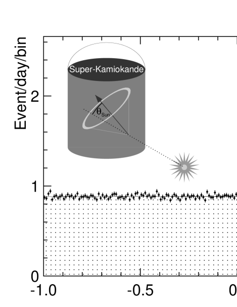
Figure 40: Angular distribution of solar neutrino event candidates. The shaded area indicates the elastic scattering peak. The dotted area is the contribution from background events.

VIII.2 Observed solar neutrino flux

Figure 40 shows the $\cos\theta_{sun}$ distribution for 1496 days of SK–I data. The best fit value for the number of signal events due to solar neutrinos between 5.0 MeV and 20.0 MeV is calculated by the maximum likelihood method in Eq. (13), and the result for SK–I is $22,404\pm 226~{}({\rm stat.})^{+784}_{-717}~{}({\rm sys.})$. The corresponding ${}^{8}B$ flux is:

$$2.35\pm 0.02~{}({\rm stat.})\pm 0.08~{}({\rm sys.})\times 10^{6}~{}{\rm cm}^{-2}{\rm s}^{-1}.$$

The systematic errors for the solar neutrino flux, seasonal variation and day-night differences for the energy range 5.0 MeV to 20.0 MeV are shown in Table 8. The detailed explanations are written in each topic’s section, but the total systematic error for the solar neutrino flux measurement is estimated to be ${}^{+3.5\%}_{-3.2\%}$.

	Flux	Seasonal	day-night
Energy scale, resolution	$\pm 1.6$	${}^{+1.2}_{-1.1}$	${}^{+1.2}_{-1.1}$
Theoretical uncertainty	${}^{+1.1}_{-1.0}$
for 8B spectrum
Trigger efficiency	${}^{+0.4}_{-0.3}$	$\pm 0.1$
Reduction	${}^{+2.1}_{-1.6}$	$\pm 0.5$
Spallation dead time	$\pm 0.2$	$\pm 0.1$	$\pm 0.1$
Gamma ray cut	$\pm 0.5$	$\pm 0.25$
Vertex shift	$\pm 1.3$
Background shape	$\pm 0.1$		$\pm 0.4$
for signal extraction
Angular resolution	$\pm 1.2$
Cross section of $\nu$-e scattering	$\pm 0.5$
Livetime calculation	$\pm 0.1$	$\pm 0.1$	$\pm 0.1$
Total	${}^{+3.5}_{-3.2}$	$\pm 0.3$	${}^{+1.3}_{-1.2}$

Table 8: Systematic error of each item (in %).

VIII.3 Time variations of solar neutrino flux

VIII.3.1 Day-Night difference

The day time flux and night time flux of solar neutrinos in SK–I are calculated using events which occurred when the solar zenith angle cosine was less than and greater than zero, respectively. The observed flux are:

$$\Phi_{day} = 2.32\pm 0.03~{}({\rm stat.})^{+0.08}_{-0.07}~{}({\rm sys.})\times 10^{6}~{}{\rm cm}^{-2}{\rm s}^{-1}$$

$$\Phi_{night} = 2.37\pm 0.03~{}({\rm stat.})^{+0.08}_{-0.08}~{}({\rm sys.})\times 10^{6}~{}{\rm cm}^{-2}{\rm s}^{-1}$$

Their difference leads to a day-night asymmetry, defined as ${\cal A}=(\Phi_{day}-\Phi_{night})/(\frac{1}{2}(\Phi_{day}+\Phi_{night}))$. We find:

$${\cal A}=-0.021\pm 0.020~{}(\rm{stat.})^{+0.013}_{-0.012}~{}(\rm{sys.})$$

Including systematic errors, this is less than $1-\sigma$ from zero asymmetry. The largest sources of systematic error in the asymmetry are energy scale and resolution (${}^{+0.012}_{-0.011}$) and the non-flat background shape of the $\cos\theta_{sun}$ distribution ($\pm 0.004$). As described in the neutrino oscillation analysis section, we can reduce the statistical uncertainty if we assume two-neutrino oscillations within the Large Mixing Angle region. The day-night asymmetry in that case is

$${\cal A}=-0.017\pm 0.016~{}(\rm{stat.})^{+0.013}_{-0.012}~{}(\rm{sys.})\pm 0.0004~{}(\rm{osc.})$$

with the final, tiny additional uncertainty due to the uncertainty of the oscillation parameters themselves. Figure 41 shows the solar neutrino flux as a function of the solar zenith angle cosine.

Figure 41: The solar zenith angle dependence of the solar neutrino flux (error bars show statistical error). The width of the night-time bins was chosen to separate solar neutrinos that pass through the Earth’s dense core (the rightmost Night bin) from those that pass through the mantle. The horizontal line shows the flux for all data.

VIII.3.2 Seasonal variation

Figure 42 shows the monthly variation of the flux, which each horizontal bin covers 1.5 months. The figure shows that the experimental operation is very stable.

Figure 42: Solar neutrino flux as a function of time. The binning of the horizontal axis is 1.5 months.

Figure 43 shows the seasonal variation of solar neutrino flux. As in Figure 42, each horizontal time bin is 1.5 months wide, but in this figure data taken at similar times during the year over the entire course of SK–I’s data taking has been combined into single bins. The 1.7% orbital eccentricity of the Earth, which causes about a 7% flux variation simply due to the inverse square law, is included in the flux prediction (solid line). The observed flux variation is consistent with the predicted annual modulation. Its $\chi^{2}$/d.o.f. is 4.7/7, which is equivalent to 69% C.L.. If we fit the eccentricity to the Earth’s orbit to the observed SK rate variation, the perihelion shift is $13\pm 18$ days (with respect to the true perihelion) and the eccentricity is $2.1\pm 0.3\%$ dnpaper . This is the world’s first observation of the eccentricity of the Earth’s orbit made with neutrinos. The total systematic error on the relative flux values in each seasonal bin is estimated to $\pm 1.3\%$. The largest sources come from energy scale and resolution (${}^{+1.2\%}_{-1.1\%}$) and reduction cut efficiency ($\pm 0.5\%$), as shown in Table 8.

Figure 43: The seasonal variation of the solar neutrino flux. The solid line is the prediction based on the eccentricity of the Earth’s orbit.

VIII.4 Energy spectrum

Figure 44 shows the expected and measured recoil electron energy spectrum. The expected spectrum is calculated by the detector simulation described in Section 6, and BP2004 is used as a solar model. The solid line shows the expected spectrum of ⁸B and hep neutrinos, and the dashed line shows the contribution of only ⁸B neutrinos.

The observed and expected event rates are summarized in Table 9 and Table 10. In these tables the reduction efficiencies listed in Fig. 38 are corrected.

The uncorrelated and correlated systematic errors for each energy bin are shown in Table 11 and Table 12, respectively.

Figure 44: Energy spectrum of the solar neutrino signal. The horizontal axis is the total energy of the recoil electrons. The vertical axis is the event rate of the observed solar neutrino signal events. The error bars are a quadrature of the statistical and uncorrelated errors. The reduction efficiencies in Fig. 38 are corrected. BP2004 SSM flux values are used for the ⁸B and hep MC fluxes in this plot. The dashed line shows the contribution of only ⁸B.

Energy	Observed rate			Expected rate
(MeV)	ALL	DAY	NIGHT	8B	hep
	$-1\leq\cos\theta_{\rm z}\leq 1$	$-1\leq\cos\theta_{\rm z}\leq 0$	$0<\cos\theta_{\rm z}\leq 1$
$5.0-5.5$	$74.7^{+6.6}_{-6.5}$	$72.1^{+9.5}_{-9.4}$	$77.1^{+9.2}_{-9.0}$	182.9	0.312
$5.5-6.0$	$65.0^{+3.3}_{-3.2}$	$64.8^{+4.7}_{-4.6}$	$65.1^{+4.6}_{-4.5}$	167.7	0.309
$6.0-6.5$	$61.5^{+2.4}_{-2.3}$	$60.2^{+3.4}_{-3.3}$	$62.6^{+3.3}_{-3.2}$	151.9	0.294
$6.5-7.0$	$54.1^{+1.7}_{-1.7}$	$54.2^{+2.4}_{-2.4}$	$53.9^{+2.4}_{-2.3}$	135.3	0.284
$7.0-7.5$	$49.4^{+1.5}_{-1.5}$	$49.2^{+2.2}_{-2.1}$	$49.6^{+2.1}_{-2.1}$	119.2	0.266
$7.5-8.0$	$44.3^{+1.4}_{-1.4}$	$44.8^{+2.0}_{-1.9}$	$43.8^{+1.9}_{-1.9}$	103.5	0.249
$8.0-8.5$	$36.3^{+1.2}_{-1.2}$	$35.7^{+1.7}_{-1.7}$	$36.8^{+1.7}_{-1.7}$	88.3	0.236
$8.5-9.0$	$28.7^{+1.0}_{-1.0}$	$26.6^{+1.5}_{-1.4}$	$30.6^{+1.5}_{-1.4}$	74.1	0.221
$9.0-9.5$	$25.0^{+0.9}_{-0.9}$	$25.4^{+1.4}_{-1.3}$	$24.6^{+1.3}_{-1.2}$	61.4	0.196
$9.5-10.0$	$20.8^{+0.8}_{-0.8}$	$20.7^{+1.2}_{-1.1}$	$20.8^{+1.2}_{-1.1}$	49.9	0.185
$10.0-10.5$	$16.2^{+0.7}_{-0.7}$	$15.7^{+1.0}_{-0.9}$	$16.7^{+1.0}_{-0.9}$	39.6	0.167
$10.5-11.0$	$11.2^{+0.6}_{-0.5}$	$10.9^{+0.8}_{-0.7}$	$11.5^{+0.8}_{-0.8}$	30.7	0.149
$11.0-11.5$	$9.85^{+0.51}_{-0.49}$	$9.65^{+0.74}_{-0.68}$	$10.03^{+0.73}_{-0.68}$	23.28	0.130
$11.5-12.0$	$6.79^{+0.42}_{-0.40}$	$7.14^{+0.63}_{-0.58}$	$6.47^{+0.58}_{-0.53}$	17.27	0.118
$12.0-12.5$	$5.13^{+0.36}_{-0.33}$	$5.05^{+0.52}_{-0.47}$	$5.21^{+0.51}_{-0.46}$	12.45	0.098
$12.5-13.0$	$3.65^{+0.30}_{-0.28}$	$3.96^{+0.46}_{-0.41}$	$3.38^{+0.41}_{-0.36}$	8.76	0.090
$13.0-13.5$	$2.46^{+0.25}_{-0.23}$	$2.56^{+0.38}_{-0.33}$	$2.37^{+0.35}_{-0.30}$	5.94	0.073
$13.5-14.0$	$2.02^{+0.22}_{-0.20}$	$1.95^{+0.32}_{-0.27}$	$2.09^{+0.32}_{-0.27}$	3.88	0.060
$14.0-15.0$	$1.72^{+0.21}_{-0.19}$	$1.60^{+0.31}_{-0.25}$	$1.85^{+0.31}_{-0.26}$	4.01	0.094
$15.0-16.0$	$0.949^{+0.157}_{-0.133}$	$0.750^{+0.218}_{-0.165}$	$1.136^{+0.238}_{-0.192}$	1.439	0.057
$16.0-20.0$	$0.341^{+0.103}_{-0.077}$	$0.240^{+0.148}_{-0.093}$	$0.423^{+0.156}_{-0.109}$	0.611	0.068

Table 9: Observed and expected event rates in each energy bin at 1 AU. The unit of the rates is events/kton/year. The errors in the observed rates are statistical only. The reduction efficiencies in Fig. 38 are corrected, and the expected event rates are for the BP2004 SSM flux values (⁸B flux is 5.79 $\times 10^{6}$, hep flux is 7.88 $\times 10^{3}$/cm²/sec). $\theta_{\rm z}$ is the angle between the z-axis of the detector and the vector from the Sun to the detector.

Energy	Observed rate							Expected rate
(MeV)	DAY	MANTLE1	MANTLE2	MANTLE3	MANTLE4	MANTLE5	CORE	8B	hep
	$\cos\theta_{\rm z}:-1\sim 0$	$0\sim 0.16$	$0.16\sim 0.33$	$0.33\sim 0.50$	$0.50\sim 0.67$	$0.67\sim 0.84$	$0.84\sim 1$
$5.5-6.5$	$127.^{+6.}_{-6.}$	$124.^{+15.}_{-15.}$	$106.^{+14.}_{-14.}$	$132.^{+13.}_{-12.}$	$146.^{+13.}_{-12.}$	$140.^{+14.}_{-13.}$	$119.^{+15.}_{-14.}$	320.	0.603
$6.5-8.0$	$149.^{+4.}_{-4.}$	$166.^{+11.}_{-10.}$	$158.^{+10.}_{-9.}$	$137.^{+8.}_{-8.}$	$150.^{+8.}_{-8.}$	$141.^{+9.}_{-9.}$	$137.^{+10.}_{-9.}$	358.	0.799
$8.0-9.5$	$87.8^{+2.6}_{-2.6}$	$90.7^{+7.2}_{-6.8}$	$92.1^{+6.7}_{-6.4}$	$90.5^{+5.8}_{-5.5}$	$99.8^{+5.9}_{-5.6}$	$90.3^{+6.4}_{-6.0}$	$88.5^{+7.0}_{-6.6}$	223.8	0.653
$9.5-11.5$	$57.1^{+1.9}_{-1.8}$	$56.5^{+5.2}_{-4.8}$	$63.3^{+5.0}_{-4.6}$	$56.8^{+4.1}_{-3.9}$	$59.6^{+4.2}_{-3.9}$	$60.1^{+4.6}_{-4.3}$	$60.9^{+5.2}_{-4.8}$	143.4	0.631
$11.5-13.5$	$18.7^{+1.0}_{-0.9}$	$20.0^{+2.8}_{-2.4}$	$13.8^{+2.3}_{-2.0}$	$15.3^{+2.0}_{-1.8}$	$19.5^{+2.2}_{-2.0}$	$17.0^{+2.3}_{-2.0}$	$20.4^{+2.7}_{-2.3}$	44.4	0.379
$13.5-16.0$	$4.28^{+0.48}_{-0.43}$	$4.78^{+1.45}_{-1.08}$	$6.97^{+1.56}_{-1.24}$	$5.82^{+1.22}_{-0.98}$	$5.58^{+1.19}_{-0.95}$	$3.70^{+1.14}_{-0.85}$	$3.93^{+1.27}_{-0.93}$	9.33	0.211

Table 10: Observed and expected event rates in each zenith-spectra data set at a one astronomical unit [AU] distance from the Sun. The unit of the rates is events/kton/year. The errors in the observed rates are statistical only. The reduction efficiencies in Fig. 38 are corrected, and the expected event rates are for the BP2004 SSM flux values. $\theta_{\rm z}$ is the angle between z-axis of the detector and the vector from the Sun to the detector.

Energy (MeV)	$5-5.5$	$5.5-6$	$6-6.5$	$6.5-7$	$7-$
Trigger efficiency	${}^{+2.5}_{-1.5}$	${}^{+0.8}_{-0.6}$	$\pm 0.1$	$\pm 0.2$
Reduction	$\pm 0.9$	$\pm 0.9$	$\pm 0.9$	$\pm 0.9$	$\pm 0.9$
Gamma ray cut	$\pm 0.1$	$\pm 0.1$	$\pm 0.1$	$\pm 0.1$	$\pm 0.1$
Vertex shift	$\pm 0.2$	$\pm 0.2$	$\pm 0.2$	$\pm 0.2$	$\pm 0.2$
Background shape	$\pm 0.6$	$\pm 0.5$	$\pm 0.1$	$\pm 0.1$	$\pm 0.1$
for signal extraction
Angular resolution	$\pm 2.3$	$\pm 1.0$	$\pm 1.0$	$\pm 1.0$	$\pm 1.0$
Cross section of	$\pm 0.2$	$\pm 0.2$	$\pm 0.2$	$\pm 0.2$	$\pm 0.2$
$\nu$-e scattering
Total	${}^{+3.5}_{-29}$	${}^{+1.7}_{-1.6}$	$\pm 1.4$	$\pm 1.5$	$\pm 1.4$

Table 11: Energy uncorrelated systematic errors for each energy bin.

Energy	Scale(%)		Resolution(%)		Theory(%)
$5.0-5.5$	$+0.1$	$0.0$	$+0.2$	$-0.2$	$+0.1$	$0.0$
$5.5-6.0$	$-0.1$	$+0.1$	$+0.2$	$-0.2$	$0.0$	$+0.1$
$6.0-6.5$	$-0.3$	$+0.2$	$+0.2$	$-0.2$	$-0.1$	$+0.1$
$6.5-7.0$	$-0.5$	$+0.4$	$+0.2$	$-0.2$	$-0.3$	$+0.2$
$7.0-7.5$	$-0.7$	$+0.6$	$+0.2$	$-0.2$	$-0.4$	$+0.4$
$7.5-8.0$	$-0.9$	$+0.9$	$+0.2$	$-0.2$	$-0.5$	$+0.5$
$8.0-8.5$	$-1.1$	$+1.1$	$+0.2$	$-0.2$	$-0.7$	$+0.7$
$8.5-9.0$	$-1.4$	$+1.4$	$+0.1$	$-0.1$	$-0.9$	$+0.9$
$9.0-9.5$	$-1.7$	$+1.8$	$+0.1$	$-0.1$	$-1.1$	$+1.1$
$9.5-10.0$	$-1.9$	$+2.1$	$0.0$	$0.0$	$-1.3$	$+1.4$
$10.0-10.5$	$-2.3$	$+2.5$	$-0.1$	$+0.1$	$-1.5$	$+1.7$
$10.5-11.0$	$-2.6$	$+2.8$	$-0.3$	$+0.2$	$-1.8$	$+2.0$
$11.0-11.5$	$-3.0$	$+3.2$	$-0.5$	$+0.4$	$-2.1$	$+2.3$
$11.5-12.0$	$-3.4$	$+3.6$	$-0.8$	$+0.7$	$-2.4$	$+2.6$
$12.0-12.5$	$-3.8$	$+4.1$	$-1.1$	$+0.9$	$-2.7$	$+3.0$
$12.5-13.0$	$-4.3$	$+4.5$	$-1.4$	$+1.3$	$-3.1$	$+3.3$
$13.0-13.5$	$-4.8$	$+5.0$	$-1.9$	$+1.7$	$-3.4$	$+3.8$
$13.5-14.0$	$-5.4$	$+5.5$	$-2.4$	$+2.2$	$-3.8$	$+4.2$
$14.0-15.0$	$-6.3$	$+6.3$	$-3.3$	$+3.1$	$-4.4$	$+5.0$
$15.0-16.0$	$-7.7$	$+7.6$	$-4.9$	$+4.7$	$-5.1$	$+6.2$
$16.0-20.0$	$-9.9$	$+10.2$	$-8.1$	$+8.2$	$-5.6$	$+8.7$

Table 12: Energy correlated systematic errors for each of the 21 energy bins.

VIII.5 Hep solar neutrino

The expected hep neutrino flux is three orders of magnitude smaller than the ⁸B solar neutrino flux. However, since the end-point of the hep neutrino spectrum is about 18.8 MeV compared to about 16 MeV for the ⁸B neutrinos, the high energy end of the ⁸B spectrum should be relatively enriched with hep neutrinos. In order to discuss the flux of hep neutrinos, the most sensitive energy region for hep neutrino was estimated, then, assuming all the signal events in this energy region were due to hep neutrinos, an upper limit of the hep solar neutrino flux was obtained. Any possible effects from neutrino oscillations were not considered in this analysis.

Figure 45 shows the expected integral energy distributions for solar neutrinos.

Figure 45: Integral energy distributions for the hep solar neutrino analysis. The horizontal axis is the energy threshold of the recoil electrons. The integration is up to 21.0 MeV. Upper plot: the vertical axis is the expected number of events in SK–I’s 1496 day final data sample after all cuts. The solid and dashed lines correspond to the hep solar neutrino only the and ⁸B+hep 90% C.L. upper limit. Lower plot: the ratio of the two histograms in the upper plot (dashed/solid).

In the high energy region, the relative hep contribution is high, but the expected number of events is small because of the limited observation time. For this analysis, the best energy aperture for the hep solar neutrinos was determined to be 18.0$\sim$21.0 MeV. In this energy region 0.90 hep solar neutrino events are expected from the predicted BP2004 SSM rate.

Applying the same signal extraction method to the data events in the 18.0$\sim$21.0 MeV region, we found $4.9\pm 2.7$ solar neutrino signal events. Assuming that all of these events are due to hep neutrinos, the 90% confidence level upper limit of the hep neutrino flux was $73\times 10^{3}$ cm^-2 s^-1. Figure 46 shows the differential energy spectrum of solar neutrino signals in the high energy region.

Figure 46: Energy spectrum of recoil electrons in the high energy region. The points show data with statistical error bars. The curves show expected spectra with various hep contributions to the best-fit ⁸B spectrum. The unit of the fluxes for the curves are $/cm^{2}/s$. The dotted and dashed curves show the spectrum with 73 and 0 ($\times 10^{3}/cm^{2}/s$) hep fluxes, respectively.

IX Solar neutrino oscillation analysis

Figure 47: The Sun’s electron density profile from the standard solar model ssm [SSM] as a function of the distance to the center (top panel), and Earth’s mass density profile (bottom panels). The left plot shows the density as a function of the distance to the Earth’s center. The right plot shows the minimum (dashed horizontal line), average (solid line) and maximum density (dashed line) a solar neutrino of zenith angle $\theta_{z}$ encounters on its path through the Earth. The electron density is obtained from this by multiplying by 0.497 mol/cm³ for the mantle and 0.468 mol/cm³ for the core.

IX.1 Introduction

Two-neutrino oscillations are so far sufficient to explain and describe all measured solar neutrino phenomena. The flavor eigenstates $\nu_{e}$ and $\nu_{x}$ (where $\nu_{x}$ is either $\nu_{\mu}$ or $\nu_{\tau}$ or an admixture of both) describe weak interactions of neutrinos and electrons or nucleons. Only solar $\nu_{e}$’s can participate in charged-current reactions, since the solar neutrino energy is below the $\mu$ mass threshold. These flavor eigenstates are related to the mass eigenstates $\nu_{1}$ and $\nu_{2}$ via the unitary mixing matrix $U$, which for two neutrinos can be expressed in terms of a single parameter, the weak mixing angle $\theta$:

$$U=\begin{pmatrix}\cos\theta&\sin\theta\cr-\sin\theta&\cos\theta\end{pmatrix}$$

In vacuum, the neutrino wavefunction oscillates in space with a frequency of $\sqrt{p^{2}+m^{2}}\approx p+m^{2}/2p$ leading to an oscillatory transition probability of the flavor eigenstates

$$p_{e\longrightarrow x}=p_{x\longrightarrow e}=\sin^{2}2\theta\sin^{2}\left(\pi\frac{L}{L_{\mbox{\small osc}}}\right)$$ (14)

where the oscillation length $L_{\mbox{\small osc}}=\frac{\pi}{1.27}\frac{E}{\Delta m^{2}}$. In a medium of matter density $\rho$, the small angle scattering of the $\nu_{e}$ flavor differs (due to the additional charged-current amplitude) from the $\nu_{x}$ flavor; this can be described with a matter potential $\Delta V(\rho)$. The transition probability is still given by Eq. (14) but with the “effective” oscillation length and mixing angle

$$L_{\mbox{\small eff}}=\frac{\pi}{1.27\sqrt{\left(2\Delta V+\frac{\Delta m^{2}}{E}\cos 2\theta\right)^{2}+\left(\frac{\Delta m^{2}}{E}\sin 2\theta\right)^{2}}}$$

$$\tan 2\theta_{\mbox{\small eff}}=\frac{\frac{\Delta m^{2}}{E}\sin 2\theta}{2\Delta V+\frac{\Delta m^{2}}{E}\cos 2\theta}$$

These relations are valid only for a constant matter potential (and therefore constant matter density). We calculate the oscillation probability by means of a numerical simulation using the position-dependent matter density profile in the Sun and Earth (shown in Figure 47).

As noted by Mikheyev, Smirnov, and Wolfenstein [MSW] msw , the matter density in the Sun (see Figure 47) is large enough for a resonance ($\Delta V=-\frac{\Delta m^{2}}{2E}\cos 2\theta$) to occur, producing effective maximal mixing ($\theta_{\mbox{\small eff}}=\frac{\pi}{4}$) even if the fundamental mixing $\theta$ is small. The solar and terrestrial matter densities influence the transition probability for solar neutrinos between $\Delta m^{2}/E\approx 10^{-9}$ eV²/MeV and $\approx 10^{-5}$ eV²/MeV [MSW range]. For the so-called Large Mixing Angle [LMA; $\theta\approx\pi/6$] MSW “solution” to the solar neutrino problem, $\Delta m^{2}$ is chosen so that the solar neutrino spectrum lies at the “end” of this range (near $10^{-5}$ eV²/MeV). It explains all observed solar neutrino interaction rates. In the case of the Small Mixing Angle [SMA; $\theta\approx 0.05$] MSW solution, which also explains all observed rates, the solar neutrino spectrum must be placed near $10^{-7}$ eV²/MeV (closer to the center of the MSW range). Other large angle solutions exist as well: the Low $\Delta m^{2}$ solution [LOW] lies near the “beginning” of the MSW range ($10^{-8}$ eV²/MeV), while the (quasi-) Vacuum [VAC] solutions are “below” the MSW range ($10^{-12}$ eV²/MeV to $10^{-11}$ eV²/MeV).

To calculate the solar neutrino interaction rate on Earth, three steps are required: (i) the probability $p_{1}$ ($p_{2}$) of a solar neutrino, which is born as $\nu_{e}$ in the core of the Sun, to emerge at the surface as $\nu_{1}$ ($\nu_{2}$), (ii) coherent or incoherent propagation of the $\nu_{1},\nu_{2}$ admixture to the surface of the Earth, (iii) the probability $p_{1e}$ ($p_{2e}$) for a $\nu_{1}$ ($\nu_{2}$) neutrino to appear as $\nu_{e}$ in the detector (after propagation through part of the Earth, if the Sun is below the horizon, using the PREM prem density profile of the Earth as shown in Figure 47). In and above the MSW range of $\Delta m^{2}/E$, the distance between the Sun and the Earth is much larger than the vacuum oscillation length, so the propagation (ii) can be assumed to be incoherent. In that case, the total survival probability of the $\nu_{e}$ flavor is

$$p_{e}=p_{1}\times p_{1e}+p_{2}\times p_{2e}=2p_{1}p_{1e}+1-p_{1}-p_{1e}$$

where $p_{1}$ and $p_{1e}$ are computed numerically. Below the MSW range, both the solar and terrestrial matter densities can be neglected. However, the distance L between the Sun and the Earth approaches the oscillation length, so (ii) must be done coherently, and the survival probability of the $\nu_{e}$ flavor is

$$p_{e}=1-p_{e\longrightarrow x}=1-\sin^{2}2\theta\sin^{2}\left(\pi\frac{L}{L_{\mbox{\small osc}}}\right)$$

using Eq. (14). Figure 48 shows (as an example) the survival probability of ⁸B neutrinos. Other solar neutrino branches may have slightly different probabilities, because the radial distributions of the neutrino production location differ.

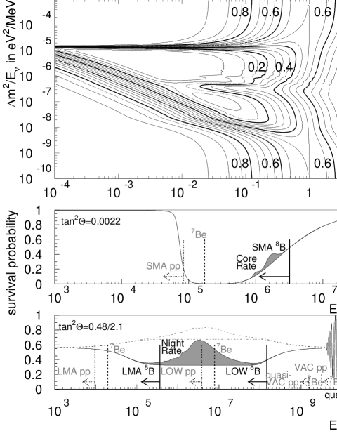
Figure 48: Survival probability for ⁸B solar neutrinos. The top plot displays contours of equal probability as a function of $\Delta m^{2}/E$ and $\tan^{2}\theta$. The middle panel shows the same probability as a function of $\Delta E/m^{2}$ only where a particular (small) mixing angle has been selected. The shaded area contrasts the difference between neutrinos passing through the core of the Earth (which has the highest matter density) with neutrinos arriving directly from the Sun. The bottom panel shows a large mixing case. The line above the shaded area depicts the average probability for neutrinos passing through the Earth. Superimposed on these two lower panels are the locations of three neutrino branches ($pp$ – dotted, ⁷Be – dashed, and ⁸B – solid) for the SMA, LMA, LOW, VAC, and quasi-VAC solutions.

Neutrino oscillations impact SK data in three independent ways: (i) Since electron neutrinos have a much larger elastic scattering cross section than other flavors, neutrino oscillations reduce the rate of solar neutrino interactions. (ii) The spectrum of recoil electrons is distorted due to the energy dependence of the survival probability. (iii) The influence of the Earth’s matter on the survival probability induces an apparent time dependence of the solar neutrino interaction rate with a 24 hour period. The amplitude of that time dependence is expressed in the day/night asymmetry $\frac{D-N}{0.5(D+N)}$ where $D$ ($N$) is the averaged interaction rate during the day (night). Due to the eccentricity of the Earth’s orbit the distance between Sun and Earth changes periodically. Since the survival probability depends on this distance (if the neutrinos propagate coherently), this leads to another time-variation (with a 365 day period) expressed in the summer/winter asymmetry $\frac{S-W}{0.5(S+W)}$ where $S$ ($W$) is the averaged interaction rate during the summer (winter), corrected for the $1/r^{2}$ dependence of the solar neutrino intensity. The day/night and summer/winter variations cannot both be present in the SK data, since above a $\Delta m^{2}$ of about $10^{-8}$ eV² neutrinos propagate incoherently and below $10^{-8}$ eV² the Earth’s matter effects on the survival probability are negligible. Figure 49 depicts the expected SK day/night asymmetry and Figure 50 the summer/winter asymmetry, depending on the oscillation parameters. They also show the SK sensitivity to distortions of the recoil electron spectrum.

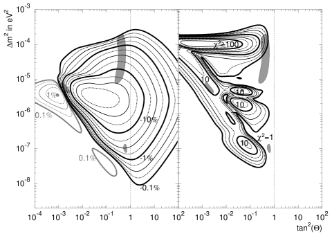
Figure 49: Expected SK day/night asymmetry (left) and spectral distortion (right) in the MSW region. The scale of the contours of equal asymmetry (distortion) is logarithmic. The spectral distortion is measured in terms of a $\chi^{2}$ using the SK spectrum uncertainties (but not the values of the SK spectrum). The gray-shaded areas correspond to the LMA, SMA, and LOW solutions.

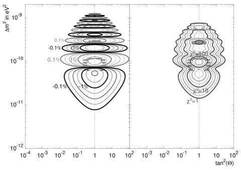
Figure 50: Expected SK summer/winter asymmetry (left) and spectral distortion (right) in the vacuum oscillation region. The scale of the contours of equal asymmetry (distortion) is logarithmic. The spectral distortion is measured in terms of a $\chi^{2}$ using the SK spectrum uncertainties (but not the values of the SK spectrum). The gray-shaded areas correspond to the VAC solutions.

Using the survival probability $p_{e}$, the neutrino interaction rate due to the neutrino spectrum $I(E_{\nu})$ at SK is

$$r_{\mbox{\tiny osc}}=\int_{E_{0}}^{E_{1}}dE\int_{E_{\nu}}dE_{\nu}I(E_{\nu})\int_{E_{e}}dE_{e}R(E_{e},E)(S_{e}(E_{\nu},E_{e})p_{e}+\hskip 28.45274pt$$

$$\hskip 170.71652ptS_{x}(E_{\nu},E_{e})(1-p_{e}))$$

where $S_{e,x}(E_{\nu},E_{e})$ describe the probability that the elastic scattering of a $\nu_{e,x}$ of energy $E_{\nu}$ with electrons produces a recoil electron of energy $E_{e}$. The Super–Kamiokande detector response is given by $R(E_{e},E)$, which describes the probability that a recoil electron of energy $E_{e}$ is reconstructed with energy $E$. The rate $r=r_{\mbox{\tiny noosc}}$ expected without oscillation is obtained by setting $p_{e}$ to 1. Since $p_{e}$ is different for each neutrino species (pp, ⁸B, hep, etc.), the calculation must be repeated for each relevant species. Due to its recoil electron energy threshold of 5.0 MeV, Super–Kamiokande–I is only sensitive to ⁸B and hep neutrinos. The oscillation analysis was performed by two methods: the first method subdivides the data sample in both recoil electron energy and solar zenith angle [Zenith Spectrum], while the second method uses only energy bins and searches for time variations by means of an unbinned likelihood [Unbinned Time Variation].

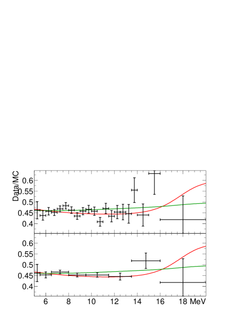
Figure 51: Distortion of the recoil electron spectrum using 21 (upper panel) and 8 (lower panel) bins. The measured event rates in each bin are divided by the event rates expected from MC assuming a ⁸B $\nu$ flux of $5.076\times 10^{6}/$cm²s and a hep $\nu$ flux of 32$\times 10^{6}/$cm²s. Overlaid is a typical LMA solution (red) and a LOW solution (green), where the assumed neutrino fluxes were fit to best describe the data.

IX.2 Analysis of the zenith spectrum $\chi^{2}$

If $B^{\mbox{\tiny osc}}_{i,z}$ ($H^{\mbox{\tiny osc}}_{i,z}$) denote the expected ⁸B (hep) neutrino induced rate in energy bin $i$ and zenith angle bin $z$ and $D_{i,z}$ the measured rate, the quantities $b$, $h$ and $d$ are defined as follows:

$$b_{i,z}=\frac{B^{\mbox{\tiny osc}}_{i,z}}{B_{i,z}+H_{i,z}}\mbox{ , }h_{i,z}=\frac{H^{\mbox{\tiny osc}}_{i,z}}{B_{i,z}+H_{i,z}}$$

$$\hskip 14.22636pt\mbox{and}\hskip 14.22636ptd_{i,z}=\frac{D_{i,z}}{B_{i,z}+H_{i,z}}.$$

For $d$, the rate calculations in the denominator use a full Monte Carlo simulation of the Super–Kamiokande detector. Figure 51 shows the average $d$ in 21 and 8 energy bins. In Figure 52, the individual $d_{i,z}$ are shown for 6 solar zenith angle bins. Now all zenith angle bins are combined into vectors. The rate difference vector

$$\overrightarrow{\Delta_{i}}(\beta,\eta)=\left(\beta\cdot\overrightarrow{b_{i}}+\eta\cdot\overrightarrow{h_{i}}\right)\times f(E_{i},\delta_{B},\delta_{S},\delta_{R})-\overrightarrow{d_{i}}$$

allows for arbitrary total neutrino fluxes through the free parameters $\beta$ and $\eta$. The combined rate predictions $\beta\overrightarrow{b_{i}}+\eta\overrightarrow{h_{i}}$ are modified by the energy-shape factors

$$f(E_{i},\delta_{B},\delta_{S},\delta_{R})=f_{B}(E_{i},\delta_{B})\times f_{S}(E_{i},\delta_{S})\times f_{R}(E_{i},\delta_{R})$$

with $\delta_{B}$ describing the ⁸B neutrino spectrum shape uncertainty, $\delta_{S}$ describing the uncertainty of the SK energy scale (0.64%) and $\delta_{R}$ describing the uncertainty of the SK energy resolution (2.5%). The $n\times n$ matrices $V_{i}$ ($n$ is the number of zenith angle bins) describe statistical and energy-uncorrelated systematic uncertainties. Those systematic uncertainties are assumed to be fully correlated in zenith angle.

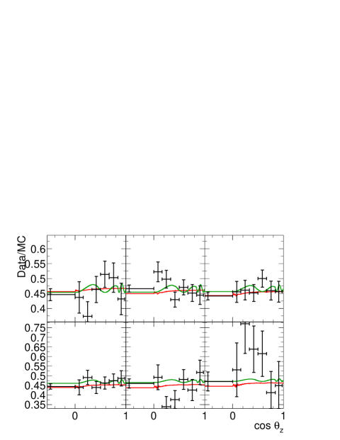
Figure 52: Dependence of Data/MC on solar zenith angle. The MC assumes a ⁸B $\nu$ flux of $5.076\times 10^{6}/$cm²s and a hep $\nu$ flux of 32$\times 10^{6}/$cm²s. The six panels correspond to the energy ranges 5.5-6.5 MeV, 6.5-8.0 MeV, 8.0-9.5 MeV, 9.5-11.5 MeV, 11.5-13.5 MeV, and 13.5-16.0 MeV. Overlaid is a typical LMA solution (red) and a LOW solution (green), where the assumed neutrino fluxes were fit to best describe the data.

To construct the $V_{i}$, we transform the rate vectors from the zenith angle basis to a new basis: the first component gives the average rate, the second component the day/night difference, the third component the difference between the rate of the mantle 1 bin and the other night bins, etc. This is achieved by multiplying $\overrightarrow{\Delta_{i}}$ by the non-singular matrix $S$ which depends on the livetimes of each zenith angle bin: $\overrightarrow{\Delta_{i}}^{\prime}=S\cdot\overrightarrow{\Delta_{i}}$

$$S=\begin{pmatrix}L_{1}/L_{1\rightarrow n}&L_{2}/L_{1\rightarrow n}&\cdots&L_{n}/L_{1\rightarrow n}\cr-1&L_{2}/L_{2\rightarrow n}&\cdots&L_{n}/L_{2\rightarrow n}\cr 0&-1&\cdots&L_{n}/L_{3\rightarrow n}\cr\vdots&\vdots&\cdots&\vdots\cr 0&\cdots&-1&1\end{pmatrix}$$

where $L_{z}$ is the livetime of zenith angle bin $z$ and $L_{z\rightarrow n}=\sum_{z^{\prime}=z}^{n}L_{z^{\prime}}$. The $\chi^{2}$ quadratic form $\overrightarrow{\Delta_{i}}^{T}\cdot V_{i}^{-1}\cdot\overrightarrow{\Delta_{i}}$ transforms as $V_{i}^{\prime}=S\cdot V_{i}\cdot S^{T}$ ($(S\cdot V_{i}\cdot S^{T})^{-1}=S^{T-1}\cdot V_{i}^{-1}\cdot S^{-1}$). Since in this new basis, the first component of $\overrightarrow{\Delta_{i}}^{\prime}$ is the livetime-averaged rate difference of energy bin $i$, the energy-uncorrelated systematic uncertainties $\sigma^{2}_{i,u}$ (assumed to be fully correlated in zenith angle) can simply be added to the statistical uncertainties $S\cdot V_{i,\mbox{\small stat}}\cdot S^{T}$:

$$S\cdot V_{i}\cdot S^{T}=S\cdot V_{i,\mbox{\small stat}}\cdot S^{T}+\begin{pmatrix}\sigma_{i,u}^{2}&0&\cdots&0\cr 0&0&\cdots&0\cr\vdots&\vdots&\cdots&\vdots\cr 0&0&\cdots&0\end{pmatrix},$$

Of course, $V_{i,\mbox{\small stat}}$ is diagonal. If $\sigma_{i,u}$ is asymmetric, two error matrices $V_{i+}$ and $V_{i-}$ are constructed. The sign of $\Delta_{i,1}^{\prime}$ (livetime-averaged rate difference) decides, if $\overrightarrow{\Delta_{i}}^{T}\cdot V_{i+}^{-1}\cdot\overrightarrow{\Delta_{i}}$ or $\overrightarrow{\Delta_{i}}^{T}\cdot V_{i-}^{-1}\cdot\overrightarrow{\Delta_{i}}$ contributes to the $\chi^{2}$

$$\chi^{2}_{0}=\sum_{i=1}^{m}\overrightarrow{\Delta_{i}}^{T}\cdot V_{i}^{-1}\cdot\overrightarrow{\Delta_{i}}$$ (15)

For any given parameters $\delta_{k}$, $\chi^{2}_{0}$ is just a quadratic form in the neutrino flux factors $\beta$ and $\eta$ and can be written as

$$\chi^{2}_{0}=\chi^{2}_{m}+\overrightarrow{\Phi}^{T}C_{0}\overrightarrow{\Phi}\hskip 14.22636pt\mbox{with}\hskip 14.22636pt\ \phi=\begin{pmatrix}\beta-\beta_{\mbox{\small min}}\cr\eta-\eta_{\mbox{\small min}}\end{pmatrix}$$

where the $2\times 2$ curvature matrix $C_{0}$ is the inverse of the covariance matrix for $\beta$ and $\eta$. This matrix $C_{0}$ must therefore be inversely proportional to the combined uncertainty of all data bins:

$$\frac{1}{\sigma_{0}^{2}}=\sum_{i=1}^{m}\frac{1}{\sigma_{\mbox{\small stat},i}^{2}+\sigma_{i,u}^{2}}\hskip 14.22636pt\mbox{with}\hskip 14.22636pt\ \frac{1}{\sigma_{\mbox{\small stat},i}^{2}}=\sum_{z=1}^{n}\frac{1}{\sigma_{\mbox{\small stat},i,z}^{2}}$$

However, the energy-uncorrelated systematic uncertainties $\sigma_{i,u}$ do not reflect the total uncertainty of the SK rate. For example, the uncertainty in the fiducial volume due to a systematic vertex shift cancels for the spectrum shape and is therefore not included in $\sigma_{i,u}$. If the spectrum data is used to constrain the total rate, the total uncertainty of that rate ($\sigma_{0}$) therefore neglects that part (called $\sigma_{r}$) of the systematic uncertainty which cancels for the spectrum. While $\sigma_{r}$ is fully correlated in both energy and zenith angle, it is not covered by the energy-correlated uncertainties either, which reflect only the uncertainties in the ⁸B neutrino spectrum, the SK energy scale, and the SK energy resolution. To take $\sigma_{r}$ into account $\chi^{2}_{0}$ is modified to

$$\chi^{2}_{1}=\chi^{2}_{m}+\overrightarrow{\Phi}^{T}C_{1}\overrightarrow{\Phi}\hskip 14.22636pt\mbox{with}\hskip 14.22636pt\ C_{1}=\frac{\sigma_{0}^{2}}{\sigma_{0}^{2}+\sigma_{r}^{2}}\times C_{0}$$

which has the same minimum as $\chi^{2}_{0}$ but allows an enlarged range of parameters $\beta,\eta$. The total $\chi^{2}$ for the SK zenith spectrum shape is then

$$\begin{matrix}\chi^{2}_{\mbox{\tiny SK}}=\mbox{Min}(&\chi^{2}_{1}(\beta,\eta,\delta_{B},\delta_{S},\delta_{R})+\cr&\left(\frac{\delta_{B}}{\sigma_{B}}\right)^{2}+\left(\frac{\delta_{S}}{\sigma_{S}}\right)^{2}+\left(\frac{\delta_{R}}{\sigma_{R}}\right)^{2})\end{matrix}$$ (16)

where all $\delta_{k}$ as well as $\beta,\eta$ are minimized. To constrain the ⁸B flux, the term $\left(\frac{\beta-1}{\sigma_{f}}\right)^{2}$ is added.

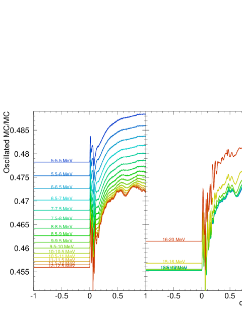
Figure 53: Predicted solar zenith angle variation assuming a typical LMA solution, $\Delta m^{2}=6.3\times 10^{-5}$ eV² and $\tan^{2}\theta=0.52$ (which is the best fit to the SK energy spectrum, rate, and day/night variation).

IX.3 Unbinned time-variation analysis

In a different approach to combine time-variation and spectrum constraints we form the total likelihood $\cal L$ modifying the solar signal factors $s_{ij}$ of Eq. (13) to

$$s_{ij}=p(\cos\theta_{ij},E_{j})\times\frac{r_{i}(t_{j})}{r^{\mbox{\tiny av}}_{i}}$$ (17)

where $t_{j}$ is the event time, $r_{i}(t)$ the predicted time dependence of the solar neutrino interaction rate in energy bin $i$, and $r^{\mbox{\tiny av}}_{i}$ the predicted time-averaged rate. Figure 53 shows the expected solar zenith angle dependence $r_{i}(\cos\theta_{z})$ in each energy bin for a typical LMA solution. The recoil electron spectrum enters this likelihood through the weight factors $Y_{i}$ of Eq. (13), so the likelihood needs to add terms like those in Eq. (16) to account for energy-correlated systematic uncertainties. The definition of energy bins is the same as in Eq. (13): This analysis uses 21 energy bins compared to 8 energy bins for the zenith spectrum.

Due to the large number of solar neutrino candidates, the maximization of this likelihood is too slow to be practical. We therefore split it into

$$\log{\cal L}=(\log{\cal L}-\log{\cal L}_{\mbox{\tiny av}})+\log{\cal L}_{\mbox{\tiny av}}$$

where ${\cal L}_{\mbox{\tiny av}}$ is the likelihood without the time variations, which means that it depends only on the average rates in each recoil electron energy bin. We can cast this in terms of a $\chi^{2}=-2\log{\cal L}$:

$$\chi^{2}=\Delta\chi^{2}_{\mbox{\tiny tv}}+\chi^{2}_{\mbox{\tiny av}}\hskip 5.69046pt\mbox{with }\Delta\chi^{2}_{\mbox{\tiny tv}}=-2(\log{\cal L}-\log{\cal L}_{\mbox{\tiny av}})$$ (18)

The first term of $\Delta\chi^{2}_{\mbox{\tiny tv}}$ uses the time-dependent solar signal factors of Eq. (17) while the second term is the same as Eq. (13). The spectrum weights $Y_{i}$ occurring in that equation are determined from the oscillated predicted spectrum. This predicted spectrum is formed using the ⁸B and hep neutrino fluxes as well as the systematic uncertainty parameters $\delta_{B}$, $\sigma_{B}$ and $\delta_{S}$. The values of these five parameters result from a fit to the (time-averaged) SK spectrum data. The dark-gray areas in Figure 54 are excluded at 95% C.L. by this $\Delta\chi^{2}_{\mbox{\tiny tv}}$.

All systematic uncertainties are assumed to be fully correlated in zenith angle or any other time variation variable. Since the sensitivity is dominated by statistical uncertainties, this assumption is not a serious limitation. We found the statistical likelihood in each energy bin $i$ to be very close to a simple Gaussian form, so $\chi^{2}_{\mbox{\tiny av}}$ takes the same form as Eq. (16) but replacing Eq. (15) with

$$\chi^{2}_{0}=\sum_{i=1}^{N_{\mbox{\tiny bin}}}\left(\frac{\Delta_{i}}{\sigma_{i}}\right)^{2}$$ (19)

where $\Delta_{i}$ has only one zenith angle bin (between $-1<\cos\theta_{z}<1$)

$$\Delta_{i}(\beta,\eta)=\left(\beta\cdot b_{i}+\eta\cdot h_{i}\right)\times f(E_{i},\delta_{B},\delta_{S},\delta_{R})-d_{i}$$

and $\sigma_{i}^{2}=\sigma_{i,\mbox{\tiny stat}}^{2}+\sigma_{i,u}^{2}$ is the total energy-uncorrelated uncertainty in that bin. The regions colored in light-gray of Figure 54 are excluded at 95% C.L. using $\chi^{2}_{\mbox{\tiny av}}$ without the term constraining the ⁸B neutrino flux.

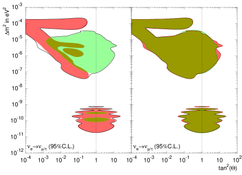
Figure 54: Left: excluded regions from the SK spectrum (red), SK rate time variations (green) and both combined (solid line) at 95% C.L.. Right: excluded regions from the SK zenith spectrum (green) compared to the SK spectrum combined with the time variation likelihood (red) at 95%C.L..

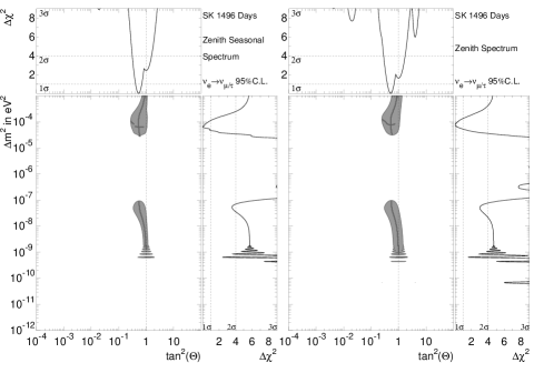
Figure 55: Allowed areas from the rate-constrained SK unbinned time-variation analysis (left) and the SK zenith spectrum (right) at 95% C.L.. The graphs at the top (and right) show the $\chi^{2}$ difference as a function of $\tan^{2}\theta$ ($\Delta m^{2}$) alone where the $\Delta m^{2}$ ($\tan^{2}\theta$) is chosen to minimize $\chi^{2}$. The lines inside the contours show which $\Delta m^{2}$ ($\tan^{2}\theta$) is chosen.

(a)                                                                          (b)

     

Figure 56: (a) Allowed area at 95% C.L from the combination of SK and SNO. The graphs at the top (and right) show the $\chi^{2}$ difference as a function of $\tan^{2}\theta$ ($\Delta m^{2}$) only: the solid line is the SK/SNO fit, the dotted line results from KamLAND kamland data. The lines inside the contours show which $\Delta m^{2}$ ($\tan^{2}\theta$) is chosen. (b) Allowed area at 95% C.L. from the combination of SK/SNO (gray) and all solar data (dark gray), and from the combination of solar and KamLAND data (light gray). Note the linear scale of both axes. Only LMA–I remains allowed. Overlaid is the region allowed by KamLAND alone .

IX.4 Oscillation constraints from SK

The combined excluded areas (from $\chi^{2}=\chi^{2}_{\mbox{\tiny av}}+\Delta\chi^{2}_{\mbox{\tiny tv}}$) at 95% C.L. are shown inside the solid line in the left panel of Figure 54. The right panel of the same figure compares these areas to the excluded areas from the zenith spectrum analysis. Both contours are quite similar, however the unbinned time-variation analysis has more stringent limits on the time-variation (note the region $10^{-6}$ eV${}^{2}<\Delta m^{2}<10^{-5}$ eV² at $\tan^{2}\theta\approx 10^{-3}$ and $\tan^{2}\theta>1$). Due to the larger number of energy bins, the likelihood analysis has also larger excluded areas in the vacuum region and at $\Delta m^{2}\approx 10^{-4}$ eV². If we include the last term in Eq. (19), we get the allowed regions (95%C.L.) shown in Figure 55 which depend on the total ⁸B neutrino flux measurement of SNO snosalt . The best fit is in the LMA region at $\tan^{2}\theta=0.52$ and $\Delta m^{2}=6.3\times 10^{-5}$ eV² ($\Delta m^{2}=7.6\times 10^{-5}$ eV²) for the unbinned time-variation analysis (zenith spectrum analysis) where a day/night asymmetry of -2.1%(-1.5%) is expected and $-1.8\pm 1.6\%$ ($-1.7\pm 1.6\%$) is found. (Here, the uncertainties do not include systematic effects). The $\chi^{2}$ is 17.3 for 20 degrees of freedom (63% C.L.). The ⁸B flux is fit to $4.91\times 10^{6}/$cm²s. The $\chi^{2}_{\mbox{\tiny av}}$ of the SK spectrum and rate is 18.5 for 20 degrees of freedom (55% C.L.). The $\chi^{2}$ analysis of the zenith spectrum gives a minimum $\chi^{2}$ of 39.0 with 43 degrees of freedom (65% C.L.). The ⁸B flux is fit to $4.86\times 10^{6}/$cm²s. Figure 55 also shows the $\chi^{2}$ as a function of $\tan^{2}\theta$ alone where a $\Delta m^{2}$ is chosen for each $\tan^{2}\theta$ to minimize $\chi^{2}$: SK data excludes small mixing at more than $3\sigma$. SK data also disfavors $\Delta m^{2}>10^{-3}$eV² and $2\times 10^{-9}$eV${}^{2}<\Delta m^{2}<3\times 10^{-5}$eV² (see the plot in the right panel, where $\chi^{2}$ is minimized with respect to $\tan^{2}\theta$). Again, the unbinned time-variation analysis has more stringent oscillation constraints and favors the LMA region more strongly.

IX.5 Combined oscillation constraints from several experiments

Stronger constraints on $\Delta m^{2}$ result from the combination of the SK measurements with other solar neutrino data. The 95% C.L. allowed region of Figure 56(a) include in addition to the SK data the SNO measurements of the charged-current interaction rate (and day/night asymmetry) of solar electron neutrinos with deuterons snoncdn ; only LMA solutions survive. Overlaid are the contours allowed by the KamLAND reactor neutrino spectrum kamland . Figure 56(b) shows the allowed contours of a combined fit to SK, SNO and KamLAND data. SK and SNO remove the ambiguities in $\Delta m^{2}$ and $\tan^{2}\theta$ of KamLAND and tighten the constraint on the mixing angle. When the charged-current rates measured by Homestake, GALLEX, and SAGE othersolar are included as well, the allowed LMA solutions are further reduced. However, in this case the fit relies on the SSM predictions of the pp, pep, CNO and ⁷Be neutrino fluxes.

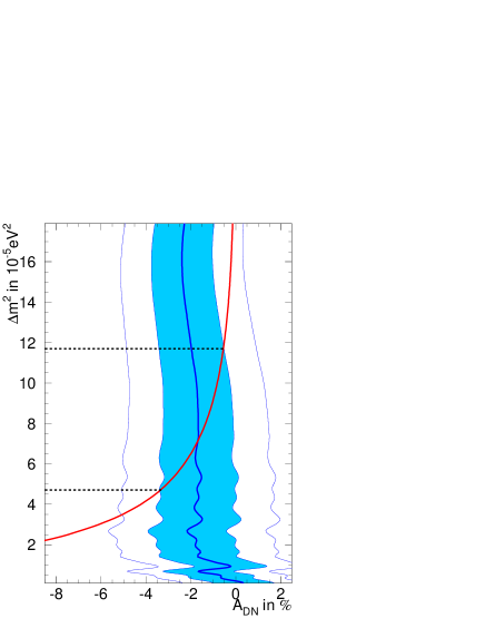
Figure 57: Day/Night amplitude fit depending on $\Delta m^{2}$. The fit depends only very weakly on the mixing angle which is assumed to be $\tan^{2}\theta=0.44$. Overlaid (red line) is the expected amplitude and (blue lines) the $2\sigma$ boundaries of the amplitude fit.

IX.6 Solar day/night effect

Even though KamLAND provides by far the best constraint on the solar $\Delta m^{2}$ it is interesting to study the solar constraints as well. The upper bound arises from the ratios of the electron–neutrino elastic scattering rate in SK, the charged-current neutrino interactions in SNO and Homestake, and the neutral-current neutrino interactions in SNO. The lower bound is due to the solar neutrino day/night effect. As described in dnpaper , we fit the amplitude of this variation to our data and compare it to the expected amplitude. For this fit, only the amplitude of the day/night variation is varied, the shape is fixed to the calculated shape for a particular $\Delta m^{2}$ and $\tan^{2}\theta$ (see Figure 53 for a typical LMA solution). Demanding consistency between expected and observed amplitude, we obtain a range of $5\times 10^{-5}$ eV${}^{2}<\Delta m^{2}<12\times 10^{-5}$ eV² at the $1\sigma$ level and a lower bound of $3\times 10^{-5}$ eV${}^{2}<\Delta m^{2}$ at the $2\sigma$ level ($\tan^{2}\theta=0.44$). This agrees very well with the KamLAND measurement of $7.9\times 10^{-5}$ eV². Conversely, if we confine $\Delta m^{2}$ to the $3\sigma$ range $7\times 10^{-5}$ eV${}^{2}<\Delta m^{2}<9\times 10^{-5}$ eV² allowed by KamLAND, the amplitude fit varies only very slightly. In that range the measured SK day/night variation amplitude corresponds to a day/night asymmetry of -1.7%$\pm$1.6%(stat)${}^{+1.3}_{-1.2}$(syst)$\pm$0.04%($\Delta m^{2}$) while the expected asymmetry ranges from -1.7% to -1.0%. At the SK best-fit $\Delta m^{2}=6.3\times 10^{-5}$ eV², the day/night amplitude fit corresponds to the asymmetry -1.8%$\pm$1.6%(stat)${}^{+1.3}_{-1.2}$(syst).

X Conclusion

Solar neutrino measurements using neutrino-electron scattering in the Super–Kamiokande detector are described. We obtained 1496 effective days of data in the time period of May 31st 1996 through July 15th 2001. The analysis threshold was 6.5 MeV for the first 280 days, and 5.0 MeV for the remaining 1216 days. The observed interaction rate corresponds to a ⁸B solar electron-neutrino flux of $2.35\pm 0.02\pm 0.08\times 10^{6}$cm^-2sec^-1. We searched for periodic time variations of this rate and found only the expected seasonal variation caused by the eccentricity of the earth’s orbit. The energy spectrum of the recoiling electron is consistent with an undistorted solar ⁸B neutrino spectrum. Based on these results the solar neutrino oscillation analysis imposes strong constraints on the oscillation parameters, selecting large mixing and favoring the Large Mixing Angle solution. The combination with data from other experiments confirms the Large Mixing Angle solution and further reduces the uncertainty in the oscillation parameters.

- (1) Present address: High Energy Accelerator Research Organization (KEK), Tsukuba, Ibaraki 305-0801, Japan
- (2) Present address: International Center for Elementary Particle Physics, University of Tokyo, Bunkyo, Tokyo 113-0033, Japan
- (3) Present address: Faculty of Science, Chiba University, Chiba, Chiba 263-8522, Japan
- (4) Present address: Department of Physics, Indiana University, Bloomington, IN 47405, USA
- (5) Present address: Center for Gravitational Wave Physics, Pennsylvania State University, University Park, PA 16802, USA
- (6) Present address: Department of Physics, Stanford University, Stanford, CA 94305, USA
- (7) Present address: Department of Physics, University of Utah, Salt Lake City, Utah 84112, USA
- (8) Present address: Fermi National Accelerator Laboratory, Batavia, IL 60510, USA
- (9) S. Fukuda et al., Nucl. Instr. Meth. A501 (2003) 418.
- (10) H.Kume et al., Nucl. Instr. Meth. 205 (1983) 299.
- (11) A.Suzuki et al., Nucl. Instr. Meth. A329 (1993) 299.
- (12) C.E. Ortiz et al., Phys. Rev. Lett. 85 (2000) 2909.
- (13) J.N.Bahcall et al., Phys. Rev. C54 (1996) 411.
- (14) J.N.Bahcall et al., Phys. Rev. D51 (1995) 6146.
- (15) A.Morel et al., Limnology and Oceanography 22 (1977) 709.
- (16) M.Nakahata, et al. Nucl. Instr. Meth. A421 (1999) 113.
- (17) E.Blaufuss, et al. Nucl. Instr. Meth. A458 (2001) 636.
- (18) M.Nemoto et al., Radioisotopes 46 (1997) 710.
- (19) Y.Takeuchi et al., Nucl. Instr. Meth. A421 (1999) 334.
- (20) C.Mitsuda et al., Nucl. Instr. Meth. A497 (2003) 414.
- (21) Y.Takeuchi et al., Phys. Lett. B452 (1999) 418.
- (22) M.B.Smy et al., Phys. Rev. D69 (2004) 011104.
- (23) J.N.Bahcall and M.H.Pinsonneault, Phys. Rev. Lett. 92 (2004) 121301.
- (24) S.P. Mikheyev and A.Y. Smirnov, Sov. J. Nucl. Pphys. 42 (1985) 913; L. Wolfenstein, Phys. Rev. D17 (1978) 2369.
- (25) A.M.Dziewonski and D.L.Anderson, Phys. Earth Planet. Inter. 25 (1981) 297.
- (26) T.Araki et al., Phys. Rev. Lett. 94 (2005) 081801.
- (27) B.Aharmim et al., nucl-ex/0502021; S.N.Ahmed et al., Phys. Rev. Lett. 92 (2004) 181301.
- (28) Q.R.Ahmed et al., Phys. Rev. Lett. 89 (2002) 011301; Q.R.Ahmed et al., Phys. Rev. Lett. 89 (2002) 011302.
- (29) B.T.Cleveland et al., Astrophys. J. 496 (1998) 505; J.N.Abdurashitov et al., Phys. Rev. C60 (1999) 055801; M.Altmann et al., Phys. Lett. B490 (2000) 16; also present at Neutrino 2004 by C.Cattadori.