TUM-HEP-553/04

Simulation of long-baseline neutrino oscillation experiments with GLoBES

(General Long Baseline Experiment Simulator)

P. Huber,  M. Lindner, and  W. Winter

^,,Institut für Theoretische Physik, Physik–Department,

Technische Universität München, James–Franck–Strasse, D–85748 Garching, Germany

We present the GLoBES (“General Long Baseline Experiment Simulator”) software package, which allows the simulation of long-baseline and reactor neutrino oscillation experiments. One part of the software is the abstract experiment definition language to define experiments with beam and full detector descriptions as accurate as possible. Many systematics options are provided, such as normalization and energy calibration errors, or the choice between spectral or total rate information. For the definition of experiments, a new transparent building block concept is introduced. In addition, an additional program provides the possibility to develop and test new experiment definitions quickly. Another part of GLoBES is the user’s interface, which provides probability, rate, and $\Delta\chi^{2}$ information for a given experiment or any combination of up to 32 experiments in C. Especially, the $\Delta\chi^{2}$ functions allow a simulation with statistics only, systematics, correlations, and degeneracies. In particular, GLoBES can handle the full multi-parameter correlation among the oscillation parameters, external input, and matter density uncertainties.

1 Introduction

Neutrino oscillations are now established as the leading flavor transition mechanism for neutrinos. In a long history of many experiments, see e.g. [1], two oscillation frequencies have been identified: The fast “atmospheric” and the slow “solar” oscillations, which are driven by the respective mass squared differences. In addition, there could be interference effects between these two oscillations, provided that the coupling given by the small mixing angle $\theta_{13}$ is large enough. Such interference effects include, for example, leptonic CP violation. In order to test the unknown oscillation parameters, i.e., the mixing angle $\theta_{13}$, the leptonic CP phase, and the neutrino mass hierarchy, new long-baseline and reactor experiments are proposed. These experiments send an artificial neutrino beam to a detector, or detect the neutrinos produced by a nuclear fission reactor. However, the presence of multiple solutions which are intrinsic to neutrino oscillation probabilities [2, 3, 4, 5] affect these measurements. Thus optimization strategies are required which maximally exploit complementarity between experiments. Therefore, a modern, complete experiment simulation and analysis tool does not only need to have a highly accurate beam and detector simulation, but also powerful means to analyze correlations and degeneracies, especially for the combination of several experiments. In this paper, we present the GLoBES software package as such a tool.

GLoBES (“General Long Baseline Experiment Simulator”) is a flexible software tool to simulate and analyze neutrino oscillation long-baseline and reactor experiments using a complete three-flavor description. On the one hand, it contains a comprehensive abstract experiment definition language (AEDL), which allows to describe most classes of long baseline and reactor experiments at an abstract level. On the other hand, it provides a C-library to process the experiment information in order to obtain oscillation probabilities, rate vectors, and $\Delta\chi^{2}$-values (cf., Fig. 1). In addition, it provides a binary program to test experiment definitions very quickly, before they are used by the application software. Currently, GLoBES is available for GNU/Linux. Since the source code is included, the modifications to other operating systems should be doable.

GLoBES allows to simulate experiments with stationary neutrino point sources, where each experiment is assumed to have only one neutrino source. Such experiments are neutrino beam experiments and reactor experiments. Geometrical effects of a source distribution, such as in the sun or the atmosphere, can not be described. In addition, sources with a physically significant time dependencies can not be studied, such as supernovæ.

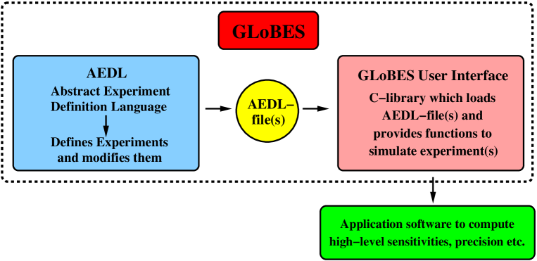
Figure 1: General concept of the GLoBES package.

On the experiment definition side, either built-in neutrino fluxes (e.g., neutrino factory) or arbitrary, user defined fluxes can be used. Similarly, arbitrary cross sections, energy dependent efficiencies, energy resolution functions as well as the considered oscillation channels, backgrounds, and many other properties can be specified. For the systematics, energy normalization and calibration errors can be simulated. Note that energy ranges and windows and bin widths can be (almost) arbitrarily chosen, including bins of different widths. Together with GLoBES comes a number of pre-defined experiments in order to demonstrate the capabilities of GLoBES and to provide prototypes for new experiments. In addition, they can be used to test new physics ideas with complete experiment simulations. Examples for these prototypes are the MINOS, ICARUS, and OPERA simulations from Ref. [6], the JHF-SK and NuMI superbeam simulations from Refs. [7, 8], the JHF-HK superbeam upgrade simulation from Ref. [7], the neutrino factory simulations from Ref. [7], and the reactor experiment simulations from Ref. [9]. Other projects using earlier versions of the GLoBES software include Refs. [10, 11, 12, 13].

With the C-library, one can extract the $\Delta\chi^{2}$ for all defined oscillation channels for an experiment or any combination of experiments. Of course, also low-level information, such as oscillation probabilities or event rates, can be obtained. GLoBES includes the simulation of neutrino oscillations in matter with arbitrary matter density profiles, as well as it allows to simulate the matter density uncertainty. As one of the most advanced features of GLoBES, it provides the technology to project the $\Delta\chi^{2}$, which is a function of all oscillation parameters, onto any subspace of parameters by local minimization. This approach allows the inclusion of multi-parameter-correlations, where external constraints (e.g., on the solar parameters) can be imposed, too. Applications of the projection mechanism include the projections onto the $\sin^{2}2\theta_{13}$-axis and the $\sin^{2}2\theta_{13}$-$\delta_{\mathrm{CP}}$-plane. In addition, all oscillation parameters can be kept free to precisely localize degenerate solutions.

2 The computation of raw event rates

In this section, we sketch the computation of the event rates, which is one of the core parts of the GLoBES software. However, because of the complexity of this issue, we refer to the GLoBES manual [14] for details.

The differential event rate for each channel is given by

$$\frac{dn_{\beta}^{\text{IT}}}{dE^{\prime}}= N\,\int\limits_{0}^{\infty}\int\limits_{0}^{\infty}dE\,d\hat{E}\quad\underbrace{\Phi_{\alpha}(E)}_{\mathrm{Production}}\times$$ (1)

$$\underbrace{\frac{1}{L^{2}}P_{(\alpha\rightarrow\beta)}(E,L,\rho;\theta_{23},\theta_{12},\theta_{13},\Delta m^{2}_{31},\Delta m^{2}_{21},\delta_{\mathrm{CP}})}_{\mathrm{Propagation}}\times$$

$$\underbrace{\sigma^{\text{IT}}_{f}(E)k_{f}^{\text{IT}}(E-\hat{E})}_{\mathrm{Interaction}}\times$$

$$\underbrace{T_{f}(\hat{E})V_{f}(\hat{E}-E^{\prime})}_{\mathrm{Detection}}\,,$$

where $\alpha$ is the initial flavor of the neutrino, $\beta$ is the final flavor, $\Phi_{\alpha}(E)$ is the flux of the initial flavor at the source, $L$ is the baseline length, $N$ is a normalization factor, and $\rho$ is the matter density. The energies in this formula are given as follows:

• $E$ is the incident neutrino energy, i.e., the actual energy of the incoming neutrino (which is not directly accessible to the experiment)

• $\hat{E}$ is the energy of the secondary particle

• $E^{\prime}$ is the reconstructed neutrino energy, i.e., the measured neutrino energy as obtained from the experiment

The interaction term is composed of two factors, which are the total cross section $\sigma^{\text{IT}}_{\beta}(E)$ for the flavor $f$ and the interaction type IT, and the energy distribution of the secondary particle $k_{\beta}^{\text{IT}}(E-\hat{E})$. The detector properties are modeled by the threshold function $T_{\beta}(\hat{E})$, coming from the the limited resolution or the cuts in the analysis, and the energy resolution function $V_{\beta}(\hat{E}-E^{\prime})$ of the secondary particle.

Since it is a lot of effort to solve this double integral numerically, we split up the two integrations. First, we evaluate the integral over $\hat{E}$, where the only terms containing $\hat{E}$ are $k_{\beta}^{\text{IT}}(E-\hat{E})$, $T_{\beta}(\hat{E})$, and $V_{\beta}(\hat{E}-E^{\prime})$. We define:

$$R_{\beta}^{\text{IT}}(E,E^{\prime})\,\epsilon_{\beta}^{\text{IT}}(E^{\prime})\equiv\int\limits_{0}^{\infty}d\hat{E}\quad T_{\beta}(\hat{E})\,k_{\beta}^{\text{IT}}(E-\hat{E})\,V_{\beta}(\hat{E}-E^{\prime})\,.$$ (2)

Thus, $R_{\beta}^{\text{IT}}(E,E^{\prime})$ describes the energy response of the detector, i.e., a neutrino with a (true) energy $E$ is reconstructed with an energy between $E^{\prime}$ and $E^{\prime}+dE^{\prime}$ with a probability $R_{\beta}^{\text{IT}}(E,E^{\prime})dE^{\prime}$. The function $R(E,E^{\prime})$ is also often called “energy resolution function”. Actually, its internal representation in the software is a smearing matrix. The function $\epsilon_{\beta}^{\text{IT}}(E^{\prime})$ will be refered to as “post-smearing efficiencies”, since it will allow us to define cuts and threshold functions after the smearing is performed, i.e., as function of $E^{\prime}$. In addition, GLoBES uses “pre-smearing efficiencies”, which are evaluated before the smearing is performed, i.e., as function of $E$. Similarly, constant background rates can be added to the event rates before or after the energy smearing, which are refered to as “pre-smearing backgrounds” and “post-smearing backgrounds”. These types of efficiencies and backgrounds allow a very accurate modeling of many factors, such as atmospheric or geoneutrino backgrounds, energy cuts, or energy threshold functions.

Eventually, we can write down the number of events per bin $i$ and channel $c$ as

$$n_{i}^{c}=\int_{E_{i}-\Delta E_{i}/2}^{E_{i}+\Delta E_{i}/2}dE^{\prime}\quad\frac{dn_{\beta}^{\text{IT}}}{dE^{\prime}}(E^{\prime})\,$$ (3)

where $\Delta E_{i}$ is the bin size of the $i$th energy bin. This means that one has to solve the integral

$$n_{i}^{c}=N/L^{2}\,\int_{E_{i}-\Delta E_{i}/2}^{E_{i}+\Delta E_{i}/2}dE^{\prime}\quad\int\limits_{0}^{\infty}dE\,\,\Phi^{c}(E)\,P^{c}(E)\,\sigma^{c}(E)\,R^{c}(E,E^{\prime})\,\epsilon^{c}(E^{\prime})\,,$$ (4)

which gives the raw event rates of the channel $c$ in the $i$th bin. Note that the events are binned according to their reconstructed energy.

Core part of the event rate computation is the energy smearing algorithm to evaluate Eq. (4), where either a particular energy resolution function can be chosen for automated energy smearing, or the discretized smearing matrix $R^{c}(E,E^{\prime})=R^{c}_{ij}$ can be given manually. In addition, it is possible to define a low-pass filter to avoid aliasing effects for neutrino oscillations faster than the sampling width.

3 Definition of experiments with AEDL
(Abstract Experiment Definition Language)

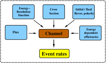
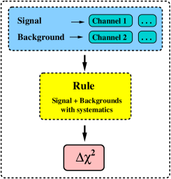
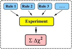
Figure 2: The most important components of AEDL: Channels, rules, and experiments.

In order to define experiments, GLoBES uses AEDL (“Abstract Experiment Definition Language”). An experiment normally corresponds to an AEDL file, which is a human readable text file written in AEDL syntax.

The key concept of AEDL is to regard a detector as an abstract system which maps the true properties of a neutrino onto the reconstructed properties of the neutrino. The latter are subsequently used in the fit of the oscillation parameters. Within GLoBES, only energy and flavor are observables, which is sufficient for long-baseline and reactor experiments. In other experiments, such as atmospheric neutrino experiments, more observables (e.g., direction) may have to be considered.

The main components of any AEDL experiment definition are “channels”, “rules”, and “experiments” (cf., Fig. 2). A channel corresponds to a neutrino oscillation channel including flux, cross section (for one specific interaction type), energy resolution function, initial and final neutrino flavors, their polarity (neutrinos or antineutrinos), and efficiencies. The channel raw event rates are computed according to Eq. (4). Each channel leads to the raw event rates for a specific interaction type. In AEDL, many of the channel components have to be defined or loaded from files before, such as fluxes, cross sections, or the energy resolution function. For the different options, see the GLoBES manual [14].

For a “rule”, the raw event rates of one or more signal channels and one or more background channels are added. The splitting in signal and background is arbitrary, but all of the signal and background components are defined to have a common systematics. The event rates of all signal and background components add up to the total event rate of the rule, which leads to a $(\Delta\chi^{2})_{r}$. The signal or background within each rule allows the specification of signal and background normalization errors and energy tilt or calibration errors. These systematical errors are evaluated with the “pull method” such as in Refs. [7, 15]. In addition to these systematics errors, an overall evaluation strategy is assigned to each rule, which specifies the type of systematics (tilt or calibration error), and the use of spectral information or total event rates.

Finally, one ore more rules add up to an experiment, where the total $\Delta\chi^{2}$ is obtained as the sum of the $(\Delta\chi^{2})_{r}$ of all rules. This approach allows the definition of appearance and disappearance channels, neutrino and antineutrino running, or interaction types with different systematics (spectral information versus counting rate) within one experiment. The GLoBES user interface allows the simulation of one or more experiment simultaneously, which means that one could also use different experiments for different oscillation channels. However, there is still one component missing in the experiment definition, which is the matter density profile. For an experiment, an arbitrary matter density profile can be specified, which is evaluated with the evolution operator method [16]. In addition, the matter density profile is multiplied by a scaling factor, which is treated as an independent parameter with a relative (matter density) uncertainty. With this approach, one can take into account that the matter density profile along a specific baseline is only known to about $3\%-5\%$. Thus, for one particular baseline, all rules should be defined within one experiment.

4 Analysis of experiments: The C user’s interface

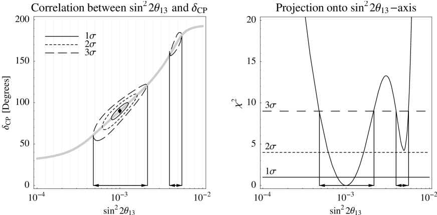
Figure 3: Left plot: Example for a correlation between $\sin^{2}2\theta_{13}$ and $\delta_{\mathrm{CP}}$ (for 1 d.o.f. only, un-shown oscillation parameters fixed). Right plot: The $\chi^{2}$-value of the projection onto the $\sin^{2}2\theta_{13}$-axis as function of $\sin^{2}2\theta_{13}$. The projection onto the $\sin^{2}2\theta_{13}$-axis is obtained by finding the minimum $\chi^{2}$-value for each fixed value of $\sin^{2}2\theta_{13}$ in the left-hand plot, i.e., along the gray vertical lines. The thick gray curve marks the position of these minima in the left-hand plot. The arrows mark the obtained fit ranges for $\sin^{2}2\theta_{13}$ at the $3\sigma$ confidence level (1 d.o.f.), i.e., the precision of $\sin^{2}2\theta_{13}$.

In order to use GLoBES, a C-library is linked with the application software. This library provides the user’s interface functions. It allows to load AEDL files, initialize the experiments, and have access to various $\Delta\chi^{2}$-functions including any combination of systematics and correlations. In addition, it provides low-level access to oscillation probabilities and event rates, and allows the readout and modification of many experiment parameters at run time.

The most sophisticated feature of the user’s interface is the possibility to include the full multi-parameter correlation among all oscillation parameters. Together with the matter densities of the $N_{\mathrm{exp}}$ loaded experiments ($N_{\mathrm{exp}}\geq 1$), the neutrino oscillation parameter space in GLoBES has $6+N_{\mathrm{exp}}$ dimensions. In the $\chi^{2}$-approach, the allowed region of $k$ ($1\leq k<6+N_{\mathrm{exp}}$) fit parameters (at the chosen confidence level) is obtained as the projection of the $6+N_{\mathrm{exp}}$-dimensional fit manifold onto the $k$-dimensional hyperplane. For example, for the precision of the parameter $\sin^{2}2\theta_{13}$ only, the fit manifold needs to be projected onto the $\sin^{2}2\theta_{13}$-axis. One can easily imagine that the computation of the full multi-parameter correlation is very expensive with a grid-based method. However, the topology of the neutrino oscillation parameter space is well investigated and rather smooth. Therefore, it is feasible to use local minimization for each solution in the parameter space. For this process, a $6+N_{\mathrm{exp}}$-dimensional local minimizer is started at the “guessed” position for the solution (such as from analytical knowledge) and then runs into a local minimum. This exercise has to be repeated till all local minima, i.e. degenerate solutions, are found. In Fig. 3, this minimization is illustrated at the simple example of a two-parameter correlation at a neutrino factory.

As we have indicated above, the matter density of each experiment is treated as an additional parameter, which is known from external measurement with a certain precision. In principle, the GLoBES user’s interface allows such externally imposed precisions for all oscillation parameters. This feature turns out to be especially useful for input from the solar neutrino experiments, since they provide better precisions for the solar neutrino oscillation parameters $\Delta m_{21}^{2}$ and $\theta_{12}$ than long-baseline experiments themselves.

5 Complexity and computational issues

The GLoBES software only uses polynomial algorithms, which are, however, suffering from the large number of dimensions. The $\Delta\chi^{2}$ computation basically consists of two steps: The systematics $(\Delta\chi^{2})_{\mathrm{sys}}$ computation with glbChiSys, and the projection algorithm which uses glbChiSys many times. The overall computation time is obtained as the product of these two steps.

The run time of the systematics $(\Delta\chi^{2})_{\mathrm{sys}}$ is

$$\mathrm{t_{sys}}=\mathcal{O}\left(N_{\mathrm{Sampling}}\times N_{\mathrm{Bins}}\,+\,N_{\mathrm{Sampling}}\times N_{\mathrm{Layers}}\right),$$ (5)

since the oscillation probabilities for all channels and energies are only computed once and stored in a list. Here $N_{\mathrm{Sampling}}$ is the number of sampling points for the evaluation of the right integral in Eq. (4), $N_{\mathrm{Bins}}$ is the number of energy bins, and $N_{\mathrm{Layers}}$ is the number of matter density layers. Thus, whenever the number of matter density steps is small, the product of sampling points and bins dominates. In practice, the $N_{\mathrm{Sampling}}\times N_{\mathrm{Bins}}$ energy smearing matrix is already computed at the experiment initialization in order to save run time. In addition, since it contains a lot of zeros, GLoBES uses a special format to avoid looping over the zeros.

The run time for the projected $\Delta\chi^{2}$ would, for a grid based method, be

$$\mathrm{t_{proj}^{Grid}}=\mathcal{O}\left(n^{6+N_{\mathrm{exp}}}\right)\,\times\,\mathrm{t_{sys}},$$ (6)

where $n$ is the number of grid points to be evaluated for each oscillation parameter, and $N_{\mathrm{exp}}$ is the number of experiments (since the matter densities of all experiments appear as parameters). Though it is, in principle, possible to use such a method with GLoBES, it is impracticable in most cases, since it would involve at least billions of steps for the complete multi-parameter correlation. The local $6+N_{\mathrm{exp}}$-dimensional minimization reduces this effort to

$$\mathrm{t_{proj}^{Minimizer}}=\mathcal{O}(1000)\,\times\,N_{\mathrm{Deg}}\,\times\,\mathrm{t_{sys}}$$ (7)

steps, where $N_{\mathrm{Deg}}$ is the number of (disconnected) local minima, i.e., the number of degeneracies (typically $\mathcal{O}(10)$).

Eventually, GLoBES needs about $10$ to $15$ seconds to compute a projected $\Delta\chi^{2}$ on a modern Pentium machine. Therefore, more sophisticated applications, such as a two dimensional plot for CP violation as function of the simulated values of $\sin^{2}2\theta_{13}$ and $\delta_{\mathrm{CP}}$ can be obtained in several hours.

6 Use of package

The GLoBES package [17] is a tar-ball which consists of the source code for the C-library providing the user’s interface, the source code for a program to test AEDL files, example C-files illustrating the use of the library, experiment prototypes in AEDL with supporting flux and cross section files, and the usual supporting files for installation and compilation. Currently, GLoBES is only provided for GNU/Linux. In addition, an extensive manual covering the user’s interface and AEDL [14] can be obtained from the web-site. GLoBES is free software and as such licensed under the GNU Public License.

The installation of GLoBES is highly automated by the use of the Autotools family and follows the usual procedures. By default a shared library libglobes.so is installed, but a static version is available, too. In addition, an executable named globes is installed. It is another possibility to install GLoBES without root privilege into a user’s home directory. During the automatic configuration process also an example Makefile is produced which can serve as a template for compiling and linking own applications against libglobes.so. This Makefile can be used to directly compile and link the examples from the manual.

AEDL files, such as the experiment prototypes, can be edited with any text editor, in order to be loaded by the users’s interface later. In addition, the globes binary allows to develop and test experiment descriptions. For example, event rate information can be quickly provided to adjust the neutrino flux normalization. For further information, we refer at this place to the GLoBES manual [14].

7 Summary and conclusions

In summary, the GLoBES software package provides powerful tools to do a full three-flavor analysis of future long-baseline and reactor experiments including systematics, correlations, and degeneracies. In addition, the abstract experiment definition language allows to define experiments at an abstract level in a highly accurate fashion. Some of the major strengths of GLoBES are the ability to quickly define new experiments, the potential to take into account the full multi-parameter correlation, the possibilities to include external input and matter density uncertainties and the ability to analyze several experiments simultaneously.

We conclude that the GLoBES software has two major target groups: Experimentalists, who want to quickly evaluate the physics potential of their setups, and theorists, who want to test new ideas or strategies with pre-defined experiments. Especially, the separation between experiment descriptions as simple text files (together with supporting files) and the application software should allow an efficient and lively interaction between those two target groups.

Acknowledgments

We would like to thank Martin Freund, who wrote the very first version of a three-flavor matter profile treatment many years ago. PH is especially thankful for the invaluable advice of Thomas Fischbacher on many design issues. In addition, we would like to thank Mark Rolinec for his help to translate the experiment descriptions into AEDL, and for creating the illustrations in this manuscript. Finally, thanks to all the people who have been pushing this project for many years, to the ones who have been continuing asking for the publication of the software, and the referees of several of our papers for suggestions which lead to improvements in the software. This work has been supported by the “Sonderforschungsbereich 375 für Astro-Teilchenphysik der Deutschen Forschungsgemeinschaft”.

References

- [1] V. Barger, D. Marfatia, and K. Whisnant, Int. J. Mod. Phys. E12, 569 (2003), and references therein, hep-ph/0308123.
- [2] G. L. Fogli and E. Lisi, Phys. Rev. D54, 3667 (1996), hep-ph/9604415.
- [3] J. Burguet-Castell, M. B. Gavela, J. J. Gomez-Cadenas, P. Hernandez, and O. Mena, Nucl. Phys. B608, 301 (2001), hep-ph/0103258.
- [4] H. Minakata and H. Nunokawa, JHEP 10, 001 (2001), hep-ph/0108085.
- [5] V. Barger, D. Marfatia, and K. Whisnant, Phys. Rev. D65, 073023 (2002), hep-ph/0112119.
- [6] P. Huber, M. Lindner, M. Rolinec, T. Schwetz, and W. Winter hep-ph/0403068.
- [7] P. Huber, M. Lindner, and W. Winter, Nucl. Phys. B645, 3 (2002), hep-ph/0204352.
- [8] P. Huber, M. Lindner, and W. Winter, Nucl. Phys. B654, 3 (2003), hep-ph/0211300.
- [9] P. Huber, M. Lindner, T. Schwetz, and W. Winter, Nucl. Phys. B665, 487 (2003), hep-ph/0303232.
- [10] P. Huber and W. Winter, Phys. Rev. D68, 037301 (2003), hep-ph/0301257.
- [11] T. Ohlsson and W. Winter, Phys. Rev. D68, 073007 (2003), hep-ph/0307178.
- [12] W. Winter, Phys. Rev. D (to be published), hep-ph/0310307.
- [13] S. Antusch, P. Huber, J. Kersten, T. Schwetz, and W. Winter (2004), hep-ph/0404268.
- [14] GLoBES manual (2004), http://www.ph.tum.de/∼globes.
- [15] G. L. Fogli, E. Lisi, A. Marrone, D. Montanino, and A. Palazzo, Phys. Rev. D66, 053010 (2002), hep-ph/0206162.
- [16] T. Ohlsson and H. Snellman, Phys. Lett. B474, 153 (2000), erratum ibidem B480, 419(E) (2000), hep-ph/9912295.
- [17] P. Huber, M. Lindner, and W. Winter, GLoBES (Global Long Baseline Experiment Simulator) software, http://www.ph.tum.de/∼globes.