Abstract

The precision and discovery potential of a neutrino factory based on muon storage rings is studied. For three-family neutrino oscillations, we analyse how to measure or severely constraint the angle $\theta_{13}$, CP violation, MSW effects and the sign of the atmospheric mass difference $\Delta m^{2}_{23}$. We present a simple analytical formula for the oscillation probabilities in matter, with all neutrino mass differences non-vanishing, which clarifies the subtleties involved in disentangling the unknown parameters. The appearance of “wrong-sign muons” at three reference baselines is considered: 732 km, 3500 km, and 7332 km. We exploit the dependence of the signal on the neutrino energy, and include as well realistic background estimations and detection efficiencies. The optimal baseline turns out to be ${\cal O}(3000$ km). Analyses combining the information from different baselines are also presented.

1 Introduction

The atmospheric [1, 2] plus solar [3] neutrino data point to neutrino oscillations [4, 5] and can be easily accommodated in a three-family mixing scenario.

Let $U$, with $(\nu_{e},\nu_{\mu},\nu_{\tau})^{T}=U\cdot(\nu_{1},\nu_{2},\nu_{3})^{T}$, be the leptonic Cabibbo-Kobayashi-Maskawa (CKM) matrix in its most conventional parametrization [6]:

$$U\equiv U_{23}U_{13}U_{12}\equiv\left(\matrix{1&0&0\cr 0&c_{23}&s_{23}\cr 0&-s_{23}&c_{23}\cr}\right)\;\left(\matrix{c_{13}&0&s_{13}e^{i\delta}\cr 0&1&0\cr-s_{13}e^{-i\delta}&0&c_{13}\cr}\right)\;\left(\matrix{c_{12}&s_{12}&0\cr-s_{12}&c_{12}&0\cr 0&0&1\cr}\right)$$ (1)

with $s_{12}\equiv\sin\theta_{12}$, and similarly for the other sines and cosines. Oscillation experiments are sensitive to the neutrino mass differences and the four parameters in the mixing matrix of Eq. (1): three angles and the Dirac CP-odd phase.

The SuperKamiokande [1] data on atmospheric neutrinos are interpreted as oscillations of muon neutrinos into neutrinos that are not $\nu_{e}$’s, with a mass gap that we denote by $\Delta m^{2}_{23}$. Roughly speaking, the measured mixing angle $\theta_{23}$ is close to maximal and $|\Delta m^{2}_{23}|$ is in the range $10^{-3}$–$10^{-2}$ eV². The solar neutrino deficit is interpreted either as MSW (matter enhanced) oscillations [5] or as vacuum oscillations (VO) [4] that deplete the original $\nu_{e}$’s, presumably in favour of $\nu_{\mu}$’s or alternatively into sterile neutrinos. The corresponding squared mass differences –${\cal O}(10^{-5}$-$10^{-4})$ eV² for the large mixing angle MSW solution (LMA-MSW), ${\cal O}(10^{-6})$ eV² for the small mixing angle MSW solution (SMA-MSW), or ${\cal O}(10^{-10})$ eV² for VO– are significantly below the range deduced from atmospheric observations. We identify this mass difference with $\Delta m^{2}_{12}$ in this parametrization. Its sign is constrained by solar data: while the SMA-MSW solution exists only for positive $\Delta m^{2}_{12}$, in the LMA-MSW range there is also a small window at negative values [7].

These oscillation signals will be confirmed and further constrained in ongoing and planned atmospheric, solar and long baseline reactor experiments [8], as well as in future long baseline accelerator neutrino experiments [9]. In a few years they will answer the question of sterile neutrinos contributing or not to present data. The MSW effect is expected to play a major role in explaining the solar deficit and both solar and reactor experiments will also clarify whether Nature has chosen the LMA-MSW rather than SMA-MSW or VO solutions.

The atmospheric neutrino parameters will be known with better precision as well. Experimental information relevant for a more precise knowledge of the atmospheric neutrino fluxes will be available [10, 11]. Also, projected long baseline accelerator experiments will improve the precision of $|\Delta m^{2}_{23}|$ and $\theta_{23}$. For instance, $|\Delta m^{2}_{23}|$ is expected to be measured at MINOS with an accuracy below $10\%$ if $|\Delta m^{2}_{23}|>3\times 10^{-3}$ eV² [12].

Nevertheless, there is a strong case for going further in the fundamental quest of the neutrino masses and mixing angles, as a necessary step to unravel the fundamental new scale(s) behind neutrino oscillations. In ten years from now no significant improvement is expected in the knowledge of:

• The angle $\theta_{13}$, which is the key between the atmospheric and solar neutrino realms, for which the present CHOOZ bound is $\sin^{2}\mbox{$\theta_{13}$}\leq 5\times 10^{-2}$ [13][14].

• The sign of $\Delta m^{2}_{23}$, which determines whether the three-family neutrino spectrum is of the “hierarchical” or “degenerate” type (i.e. only one heavy state and two almost degenerate light ones, or the reverse).

• Leptonic CP-violation.

• The precise study of matter effects in the $\nu$ propagation through the Earth: a model-independent experimental confirmation of the MSW effect will not be available.

The most sensitive method to study these topics is to measure the transition probabilities involving $\nu_{e}$ and $\bar{\nu}_{e}$, in particular $\nu_{e}(\bar{\nu}_{e})\rightarrow\nu_{\mu}(\bar{\nu}_{\mu})$. This is precisely the golden measurement at the neutrino factory [15]. Such a facility is unique in providing high energy and intense $\nu_{e}(\bar{\nu}_{e})$ beams coming from positive (negative) muons which decay in the straight sections of a muon storage ring [16]. Since these beams contain also $\bar{\nu}_{\mu}(\nu_{\mu})$ (but no $\nu_{\mu}(\bar{\nu}_{\mu})$!), the transitions of interest can be measured by searching for “wrong-sign” muons: negative (positive) muons appearing in a massive detector with good muon charge identification capabilities.

The first exploratory studies of the use of a neutrino beam with these characteristics [17] were done in the context of two-family mixing. In this approximation, the wrong-sign muon signal in the atmospheric range is absent, since the atmospheric oscillation is $\nu_{\mu}\leftrightarrow\nu_{\tau}$. The enormous physics reach of such signals in the context of three-family neutrino mixing was first realized in [18], where the authors put the emphasis on the measurement of the angle $\theta_{13}$ and CP-violation (see also [19]). The latter may be at reach if the solar deficit corresponds to the LMA-MSW solution [18, 20, 21]. Recently, it has also been shown [24] that the precision in the knowledge of the atmospheric parameters $\theta_{23}$ and $|\Delta m^{2}_{23}|$ can reach the percent level at a neutrino factory, using muon disappearance measurements. Furthermore, it was pointed out [22, 23, 24] that the sign of $\Delta m^{2}_{23}$ can also be determined at long baselines, through sizeable matter effects. The importance of measuring precisely Earth matter effects in a clean and model-independent way, both for the understanding of the fundamental parameters and for their intrinsic interest has been stressed in refs. [25, 26, 27, 28].

The aim of this paper is to identify the optimal baselines for studying the above itemized topics. This requires to include in the analysis the maximum information that can be attained at any fixed baseline. While all previous analyses have been based in energy-integrated quantities, we will take into account the neutrino energy dependence of the wrong-sign muon signals, together with the information obtained from running in the two different beam polarities.

We will consider in turn scenarios in which the solar oscillation lies in the SMA-MSW or VO range and in the LMA-MSW range. In the latter, the dependence of the oscillation probabilities on the solar parameters $\theta_{12},\Delta m^{2}_{12}$, and on the CP-odd phase, $\delta$, is sizeable at terrestrial distances and complicates the measurement of $\theta_{13}$ due to the presence of other unknowns (mainly $\delta$). This potential difficulty was first pointed out in [20]. The previous analysis of the sensitivity to $\theta_{13}$ [18] neglected solar parameters and is thus only valid for the SMA-MSW and VO solutions, or the LMA-MSW if $\theta_{13}$ is large enough. In the present paper a higher statistics is considered, allowing to explore smaller values of $\theta_{13}$, and the remark is very pertinent. We will discuss in detail the issue of how to disentangle $\theta_{13}$ and $\delta$, guided by an approximate analytical formula for the oscillation probabilities in matter including two distinct mass differences. As we will see, the choice of the correct baseline is essential to solve this problem.

We shall consider the following “reference set-up”: neutrino beams resulting from the decay of $2\times 10^{20}\mu^{+}$’s and/or $\mu^{-}$’s per year in a straight section of an $E_{\mu}=50$ GeV muon accumulator. A long baseline (LBL) experiment with a 40 kT detector and five years of data taking for each polarity is considered. Alternatively, the same results could be obtained in one year of running for the higher intensity option of the machine, providing $10^{21}$ useful $\mu^{+}$’s and $\mu^{-}$’s per year. A realistic detector of magnetized iron [29] will be considered and detailed estimates of the corresponding expected backgrounds and efficiencies included in the analysis. Three reference detector distances are discussed: 732 km, 3500 km and 7332 km.

A preliminary version of this work was presented in [30].

2 Fluxes and charged currents.

2.1 The Neutrino Factory

One of the most encouraging outcomes of the recent neutrino factory workshop at Lyon [31] was the convergence of the various machine designs existing previously, to an essentially unified design [32], based on a muon accumulator with either a triangular or a bow-tie shape. Both geometries permit two straight sections pointing in different directions, allowing two different baselines.

It was also agreed in Lyon that the beam power on target should not exceed 4 MW. This, in turn, limits the production of muons to $10^{21}$ per year, out of which only 20-25 % are useful (that is, decay in the straight sections pointing towards the detectors). Agreement was also found upon other important parameters, namely the machine dual polarity (i.e, the ability to store $\mu^{+}$ and $\mu^{-}$, although not simultaneously) and the maximum realistic energy to accelerate the stored muons, which was fixed at 50 GeV.

Ultimate sensitivity to the neutrino mixing matrix parameters, in particular to $\theta_{13}$  and $\delta$, require a data set as large as possible. The analysis presented in this paper assumes a total data set of $10^{21}$ useful $\mu^{+}$ decays and $10^{21}$ useful $\mu^{-}$ decays.

2.2 Number of events

In the muon rest-frame, the distribution of muon antineutrinos (neutrinos) and electron neutrinos (antineutrinos) in the decay $\mu^{\pm}\rightarrow e^{\pm}+\nu_{e}(\bar{\nu}_{e})+\bar{\nu}_{\mu}(\nu_{\mu})$ is given by:

$$\frac{d^{2}N}{dxd\Omega}=\frac{1}{4\pi}[f_{0}(x)\mp{\cal P}_{\mu}f_{1}(x)\cos\theta]\,,$$ (2)

where $E_{\nu}$ denotes the neutrino energy, $x=2E_{\nu}/m_{\mu}$ and ${\cal P}_{\mu}$ is the average muon polarization along the beam directions. $\theta$ is the angle between the neutrino momentum vector and the muon spin direction and $m_{\mu}$ is the muon mass. The positron (electron) flux is identical to that for muon neutrinos (antineutrinos), when the electron mass is neglected. The functions $f_{0}$ and $f_{1}$ are given in Table 1 [33].

	$f_{0}(x)$	$f_{1}(x)$
$\nu_{\mu},\rm{e}$	$2x^{2}(3-2x)$	$2x^{2}(1-2x)$
$\nu_{e}$	$12x^{2}(1-x)$	$12x^{2}(1-x)$

Table 1: Flux functions in the muon rest-frame as in ref. [33].

In the laboratory frame, the neutrino fluxes, boosted along the muon momentum vector, are given by:

$$\frac{d^{2}N_{\bar{\nu}_{\mu},\nu_{\mu}}}{dyd\Omega} = \frac{4n_{\mu}}{\pi L^{2}m_{\mu}^{6}}\,\ E_{\mu}^{4}y^{2}\,(1-\beta\cos\varphi)\,\,\left\{\left[3m_{\mu}^{2}-4E_{\mu}^{2}y\,(1-\beta\cos\varphi)\right]\right.$$

$$\left.\mp\,{\cal P}_{\mu}\left[m_{\mu}^{2}-4E_{\mu}^{2}y\,(1-\beta\cos\varphi)\right]\right\}\,,$$

$$\frac{d^{2}N_{\nu_{e},\bar{\nu}_{e}}}{dyd\Omega} = \frac{24n_{\mu}}{\pi L^{2}m_{\mu}^{6}}\,\,E_{\mu}^{4}y^{2}\,(1-\beta\cos\varphi)\,\,\left\{\left[m_{\mu}^{2}-2E_{\mu}^{2}y\,(1-\beta\cos\varphi)\right]\right.$$ (3)

$$\left.\mp\,{\cal P}_{\mu}\left[m_{\mu}^{2}-2E_{\mu}^{2}y\,(1-\beta\cos\varphi)\right]\right\}\,.$$

Here, $\beta=\sqrt{1-m^{2}_{\mu}/E^{2}_{\mu}}$, $E_{\mu}$ is the parent muon energy, $y=E_{\nu}/E_{\mu}$, $n_{\mu}$ is the number of useful muons per year obtained from the storage ring and $L$ is the distance to the detector. $\varphi$ is the angle between the beam axis and the direction pointing towards the detector, assumed to be located in the forward direction of the muon beam. The angular divergence will be taken as constant, $\delta\varphi\sim 0.1$ mr.

Unlike traditional neutrino beams obtained from $\pi$ and $K$ decays, the fluxes in Eq. (3), in the forward direction, present a leading quadratic dependence on $E_{\nu}$. As a consequence, the oscillation signal does not decrease with increasing $E_{\mu}$. In Appendix A we present our numerical results for the $\nu_{e}(\bar{\nu}_{e})$ and $\bar{\nu}_{\mu}(\nu_{\mu})$ fluxes.

The charged current neutrino and antineutrino interaction rates can be computed using the approximate expressions for the neutrino-nucleon cross sections with an isoscalar target,

$$\sigma_{\nu N}\approx 0.67\times 10^{-42}\times\frac{E_{\nu}}{{\rm GeV}}\times{\rm m^{2}}~{},\qquad\sigma_{\bar{\nu}N}\approx 0.34\times 10^{-42}\times\frac{E_{\nu}}{{\rm GeV}}\times{\rm m^{2}}.$$ (4)

It follows that the number of charged current (CC) events at a neutrino factory scales cubically with energy. In Appendix A we also include our numerical results for the rates of $e^{\pm}$ and $\mu^{\mp}$ production, from a $\mu^{\mp}$ beam.

3 Oscillation Probabilities

3.1 In vacuum

Atmospheric or terrestrial experiments have an energy range such that $\Delta m^{2}\,L/E_{\nu}\ll 1$ for the smaller ($\Delta m_{12}^{2}$) but not necessarily for the larger ($\Delta m_{23}^{2}$) of these mass gaps. Even then, solar and atmospheric transitions are not (provided $\mbox{$\theta_{13}$}\neq 0$) two separate two-generation oscillations. For $|\Delta m_{12}^{2}|\ll|\Delta m_{23}^{2}|$, neutrino oscillation probabilities at terrestrial distances are accurately described by only three parameters, $\theta_{23}$, $\Delta m_{23}^{2}=\Delta m_{13}^{2}$ and $\theta_{13}$:

$$P_{\nu_{e}\nu_{\mu}(\bar{\nu}_{e}\bar{\nu}_{\mu})} = s^{2}_{23}\,\sin^{2}2\mbox{$\theta_{13}$}\,\sin^{2}\left(\frac{\mbox{$\Delta_{13}$}\,L}{2}\right)\,,$$ (5)

$$P_{\nu_{e}\nu_{\tau}(\bar{\nu}_{e}\bar{\nu}_{\tau})} = c^{2}_{23}\,\sin^{2}2\mbox{$\theta_{13}$}\,\sin^{2}\left(\frac{\mbox{$\Delta_{13}$}\,L}{2}\right)\,,$$ (6)

$$P_{\nu_{\mu}\nu_{\tau}(\bar{\nu}_{\mu}\bar{\nu}_{\tau})} = c^{4}_{13}\,\sin^{2}2\mbox{$\theta_{23}$}\,\sin^{2}\left(\frac{\mbox{$\Delta_{13}$}\,L}{2}\right)\,,$$ (7)

where

$$\Delta_{ij}\equiv\frac{\Delta m^{2}_{ij}}{2E_{\nu}}\,.$$ (8)

Eqs. (7) are a very good approximation when the solar parameters lie in the SMA-MSW or VO range. The present best fit value for $\theta_{13}$ is in the range $6^{\circ}$–$8^{\circ}$[34, 35], although it is compatible with zero within errors. Among the transitions in Eq. (7) the channels $\nu_{e}\rightarrow\nu_{\mu},\nu_{\tau}$ have clearly the best sensitivity to a small $\theta_{13}$. Experimentally, the measurement of $\nu_{e}\rightarrow\nu_{\mu}$ oscillations through the appearance of wrong-sign muons is far superior to that of $\nu_{e}\rightarrow\nu_{\tau}$ oscillations through $\tau$ detection. In [18], it was shown that the sensitivity to $\theta_{13}$ of the former can improve the present limits, which are mainly set by Chooz [13], by at least two orders of magnitude.

At the neutrino factory, precision measurements for $|\Delta m_{23}^{2}|$ and $\theta_{23}$ can also be performed. Measurements of $\tau$ appearance or $\mu$ disappearance may be competitive with wrong-sign $\mu$ signals for small values of $\theta_{13}$, because of the cosine dependence of the corresponding probabilities in Eqs. (7). We do not develop this topic further in the present work, see [24].

In the LMA-MSW scenario, for which the effects of $\Delta m^{2}_{12}$ may be relevant at the neutrino factory, a good and simple approximation for the $\nu_{e}\rightarrow\nu_{\mu}$ transition probability is obtained by expanding to second order in the small parameters, $\mbox{$\theta_{13}$},\Delta_{12}/\Delta_{13}$ and $\Delta_{12}L$:

$$P_{\nu_{e}\nu_{\mu}(\bar{\nu}_{e}\bar{\nu}_{\mu})} = s_{23}^{2}\,\sin^{2}2\mbox{$\theta_{13}$}\,\sin^{2}\left(\frac{\mbox{$\Delta_{13}$}\,L}{2}\right)+c_{23}^{2}\,\sin^{2}2\theta_{12}\,\sin^{2}\left(\frac{\Delta_{12}\,L}{2}\right)$$ (9)

$$+ \tilde{J}\,\cos\left(\pm\delta-\frac{\mbox{$\Delta_{13}$}\,L}{2}\right)\;\frac{\Delta_{12}\,L}{2}\sin\left(\frac{\mbox{$\Delta_{13}$}\,L}{2}\right)\,,$$

where here and throughout the paper the upper/lower sign in the formulae refers to neutrinos/antineutrinos, and

$$\tilde{J}\equiv c_{13}\,\sin 2\theta_{12}\sin 2\mbox{$\theta_{23}$}\sin 2\mbox{$\theta_{13}$}$$ (10)

is the usual combination of mixing angles appearing in the Jarlskog determinant. The first term in Eq. (9) is quadratic in $\sin\mbox{$\theta_{13}$}$, whereas the leading term in $\Delta_{12}$ is linear. The latter may then be significant or even dominant for very small values of $\theta_{13}$ [20], when $\Delta m^{2}_{12}$ and $\theta_{12}$ are in the range allowed by the LMA-MSW solution.

At “short” distances, such as 732 km, Eq. (9) can be further approximated by:

$$P_{\nu_{e}\nu_{\mu}(\bar{\nu}_{e}\bar{\nu}_{\mu})}=s_{23}^{2}\,\sin^{2}2\mbox{$\theta_{13}$}\left(\frac{\mbox{$\Delta_{13}$}\,L}{2}\right)^{2}+\tilde{J}\,\cos\delta\;\frac{\Delta_{12}\,L}{2}\frac{\mbox{$\Delta_{13}$}\,L}{2}+c_{23}^{2}\sin^{2}2\theta_{12}\left(\frac{\Delta_{12}\,L}{2}\right)^{2}.$$ (11)

The CP-odd term in the probability (i.e. the one proportional to $\sin\delta$) has dropped because it is of higher order in $\Delta_{ij}\,L$. The comparison of the two polarities is then not useful (except for doubling the statistics ), since the CP-conjugated channels measure the same probability. Furthermore, all terms in Eq. (11) have the same dependence on the neutrino energy and the baseline, and consequently is very hard to disentangle them. As a result we expect a large correlation between the parameters $\theta_{13}$, $\delta$, $\Delta_{12}$. Even though long baseline (LBL) reactor experiments [36] will provide a measurement of $|\Delta m^{2}_{12}|$ if the LMA-MSW solution is at work, the parameters $\theta_{13}$ and $\delta$ will have to be determined simultaneously at the neutrino factory. It will then be necessary to go to longer baselines where the energy dependence of the different terms in Eq. (9) differs, and where the comparison of the neutrino and antineutrino probabilities provides non-trivial information to separate $\delta$ from $\theta_{13}$.

It is uncertain [7] whether solar experiments will determine the sign of $\Delta m^{2}_{12}$ if it lies in the LMA-MSW range. If it remains unknown, it implies an ambiguity in the determination of $\delta$: to reverse the sign of $\Delta m^{2}_{12}$ in Eq. (9) is equivalent to replacing $\delta$ by $\delta+\pi$. Notice, though, that whether there is CP-violation or not is independent of whether the phase in any parametrization is $\delta$ or $\delta+\pi$.

It is possible to construct a measurable CP-odd asymmetry, which in vacuum is proportional to $\sin\delta$. In refs. [18] and [21], the authors considered the following integrated asymmetry (see also [37]):

$${\bar{A}}^{CP}_{e\mu}=\frac{\{N[\mu^{-}]/N_{o}[e^{-}]\}_{+}-\{N[\mu^{+}]/N_{o}[e^{+}]\}_{-}}{\{N[\mu^{-}]/N_{o}[e^{-}]\}_{+}+\{N[\mu^{+}]/N_{o}[e^{+}]\}_{-}}\,.$$ (12)

The sign of the decaying muons is indicated by a subindex, $N[\mu^{+}](N[\mu^{-}])$ are the measured number of wrong-sign muons, and $N_{o}[e^{+}](N_{o}[e^{-}])$ are the expected number of $\bar{\nu}_{e}(\nu_{e})$ charged current interactions in the absence of oscillations. The significance of this asymmetry (i.e. the asymmetry divided by its statistical error) scales with the baseline and neutrino energy in the following way:

$$\frac{{\bar{A}}^{CP}}{\delta{\bar{A}}^{CP}}\propto\sqrt{E_{\nu}}\,\left|\,\sin\left(\frac{\mbox{$\Delta_{23}$}\,L}{2}\right)\right|\,.$$ (13)

The best sensitivity to a non-zero CP-odd asymmetry is found at the maximum of the atmospheric oscillation. At the corresponding distance, however, matter effects are already important and should be taken into account, as we proceed to discuss in the next subsection.

3.2 In matter

Of all neutrino species, only $\nu_{e}$ and $\bar{\nu}_{e}$ have charged-current elastic scattering amplitudes on electrons. This, as is well known, induces effective “masses” $\mu=\pm\,2\,E_{\nu}\,A$, where the signs refer to $\nu_{e}$ and $\bar{\nu}_{e}$ and $A$ is the matter parameter,

$$A=\sqrt{2}\,G_{F}\,n_{e}\,,$$ (14)

with $n_{e}$ the ambient electron number density [5].

Matter effects may be important if $A$ is comparable to, or bigger than, the quantity $\Delta_{ij}$ for some mass difference and neutrino energy, and if distances are large enough for the probabilities to be in the non-linear region of the oscillation.

For the Earth’s crust, with density $\rho\sim$ 2.8 g/cm³ and roughly equal numbers of protons, neutrons and electrons, $A\sim 10^{-13}$ eV. The typical neutrino energies we are considering are tens of GeVs. For instance, for $E_{\nu}=30$ GeV (the average $\bar{\nu}_{e}$ energy in the decay of $E_{\mu}=50$ GeV muons) $A=1.1\times 10^{-4}$ eV²/GeV $\sim\mbox{$\Delta_{23}$}$. This means that matter effects will be important at long distances. Notice that at $L=$ 732 km and 3500 km the neutrino path remains in the Earth crust, whereas for 7332 km the deeper flight path meets a denser medium and $A=1.5\times 10^{-4}$ eV²/GeV.

3.2.1 Neglecting solar parameters: VO or SMA-MSW solutions

Consider the case when $\Delta_{12}$ is negligible compared to $\Delta_{23}$, $L^{-1}$ and A. In the approximation of constant $n_{e}$, the transition probability in matter governing the appearance of wrong-sign muons can then be read from [38]:

$$P_{\nu_{e}\nu_{\mu}(\bar{\nu}_{e}\bar{\nu}_{\mu})}\simeq s_{23}^{2}\,\sin^{2}2\mbox{$\theta_{13}$}\left(\frac{\mbox{$\Delta_{13}$}}{B_{\mp}}\right)^{2}\,\sin^{2}\left(\frac{B_{\mp}\,L}{2}\right)\ ,$$ (15)

where

$$B_{\mp}\equiv\sqrt{\left[\mbox{$\Delta_{13}$}\,\cos 2\mbox{$\theta_{13}$}\mp A\right]^{2}+\left[\mbox{$\Delta_{13}$}\,\sin 2\mbox{$\theta_{13}$}\right]^{2}}\,.$$ (16)

For $A=0$, Eq. (15) reduces to the corresponding vacuum result: the first line in Eq. (7). At short distances, that is for $B_{\mp}\,L/2$ sufficiently small, the sinus in Eq. (15) can be expanded and

$$P_{\nu_{e}\nu_{\mu}(\bar{\nu}_{e}\bar{\nu}_{\mu})}\sim s_{23}^{2}\,\sin^{2}2\mbox{$\theta_{13}$}\,\left(\frac{\mbox{$\Delta_{13}$}\,L}{2}\right)^{2}\,,$$ (17)

which also coincides with the vacuum behaviour for small $\mbox{$\Delta_{13}$}\,L/2$, even when $A\gg$ $\mbox{$\Delta_{13}$}\cos 2\mbox{$\theta_{13}$}$. Eq. (17) is a good approximation up to $\sim$ 3000 km [18]. Note that the leading dependence on $\theta_{13}$ is quadratic as in vacuum.

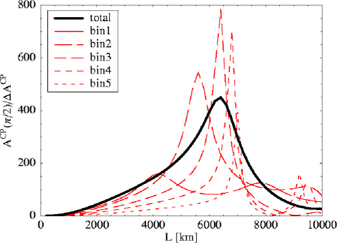
Figure 1: The signal-over-noise ratio of the CP-odd asymmetry of Eq. (12) as a function of the distance. The thick line corresponds to the integrated asymmetry, while the dashed lines correspond to the asymmetry computed in five energy bins of equal width $\Delta E_{\nu}=10$ GeV. The neutrino mixing parameters correspond to the SMA-MSW solution to the solar anomaly: $\Delta m_{23}^{2}=2.8\times 10^{-3}$ eV², $\Delta m_{12}^{2}=6\times 10^{-6}$ eV², $\sin^{2}2\theta_{12}=6\times 10^{-3}$, $\mbox{$\theta_{23}$}=45^{\circ}$, $\mbox{$\theta_{13}$}=13^{\circ}$ and $\delta=90^{\circ}$. The muon energy is $E_{\mu}=$ 50 GeV and the matter parameter $A$ is varied with the distance as in [39].

In contrast with the vacuum result, the probability in matter depends on the sign of $\Delta m^{2}_{13}$. It follows from Eqs. (15) and (16) that a change on this sign is equivalent to a CP transformation, that is, interchanging the probability of neutrinos and antineutrinos. Thus matter effects induce by themselves a non-vanishing CP-odd asymmetry, and the best sensitivity to the sign is achieved when the sensititivity to the asymmetry of Eq. (12) is maximal. Fig. 1 shows the significance of this asymmetry as a function of the baseline. The maximum sensitivity to the sign is thus expected at ${\cal O}(7000)$ km, although it is already very good at much shorter distances: notice the large number of standard deviations in the $y$ axis.

It is important to stress that having sizeable matter effects does not necessarily imply having sensitivity to the sign. For example if $A\gg\mbox{$\Delta_{13}$}\cos 2\mbox{$\theta_{13}$}$, the sensitivity is lost, even though matter effects are important at large distances. The optimal sensitivity occurs for $A\sim\mbox{$\Delta_{13}$}\cos 2\mbox{$\theta_{13}$}$, which is an energy dependent condition. In Fig. 1 the asymmetry resulting from each of five energy bins of width $\Delta E_{\nu}=10$ GeV is also shown: the asymmetries in different bins peak at different distances. This dependence suggests that using the information in energy bins can further improve the measurement of the sign of $\Delta m^{2}_{23}$.

3.2.2 With solar parameters: LMA-MSW solution

In the LMA-MSW solar scenario, the effects of $\Delta m^{2}_{12}$ are not negligible over terrestrial distances, given the high intensity of the neutrino factory. The exact oscillation probabilities in matter when no mass difference is neglected have been derived analytically in [40]. However, the physical implications of the formulae in [40] are not easily derived. A convenient and precise approximation is obtained by expanding to second order in the following small parameters: $\theta_{13}$, $\Delta_{12}/\mbox{$\Delta_{23}$}$, $\Delta_{12}/A$ and $\Delta_{12}\,L$. The result is (details of the calculation can be found in appendix C):

$$P_{\nu_{e}\nu_{\mu}(\bar{\nu}_{e}\bar{\nu}_{\mu})} = s_{23}^{2}\sin^{2}2\mbox{$\theta_{13}$}\,\left(\frac{\mbox{$\Delta_{13}$}}{\tilde{B}_{\mp}}\right)^{2}\,\sin^{2}\left(\frac{\tilde{B}_{\mp}\,L}{2}\right)\,+\,c_{23}^{2}\sin^{2}2\theta_{12}\,\left(\frac{\Delta_{12}}{A}\right)^{2}\,\sin^{2}\left(\frac{A\,L}{2}\right)$$ (18)

$$+ \tilde{J}\;\frac{\Delta_{12}}{A}\,\frac{\mbox{$\Delta_{13}$}}{\tilde{B}_{\mp}}\,\sin\left(\frac{AL}{2}\right)\,\sin\left(\frac{\tilde{B}_{\mp}L}{2}\right)\,\cos\left(\pm\delta-\frac{\mbox{$\Delta_{13}$}\,L}{2}\right)\,,$$

where $\tilde{B}_{\mp}\equiv|A\mp\mbox{$\Delta_{13}$}|$. Once again, this expression reduces to the vacuum result, Eq. (9), in the limit $A\rightarrow 0$. As already remarked in the previous subsection, a reversal of the sign of $\Delta_{12}$ in Eq. (18) can be simply traded by an shift of $\pi$ in $\delta$, and we will stick to positive $\Delta_{12}$ in the numerical exercises below.

We have numerically compared Eq. (18) with the exact formulae of [40], in the range $1^{\circ}<\mbox{$\theta_{13}$}<10^{\circ}$. Consider for instance the average energy $E_{\nu}=30$ GeV and the following set of values: $\Delta m_{23}^{2}=2.8\times 10^{-3}$ eV², $\theta_{12}=22.5^{\circ}$, $\mbox{$\theta_{23}$}=45^{\circ}$ and $\delta=90^{\circ}$. For $\Delta m_{12}^{2}=1\times 10^{-4}$ eV², the difference is $<$ 10 % ($<$ 20 %) at $L\sim$ 3000 (7000) km. For $\Delta m_{12}^{2}=1\times 10^{-5}$ eV², the error diminishes to $<$ 2.5 % ($<$ 10 %) at $L\sim$ 3000 (7000) km. Slightly better accuracy is obtained for $\delta=0^{\circ}$.

As before, matter effects in Eq. (18) induce an asymmetry between neutrinos and antineutrinos oscillation probabilities even for vanishing $\delta$. For this reason the CP-odd asymmetry, Eq. (12), is not the most transparent observable to determine the optimal distance for measuring $\delta$. A better way of addressing the issue is to ask at what distance the significance of the terms which depend on $\delta$ is maximal.

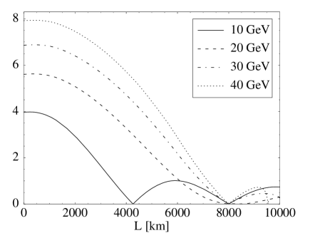
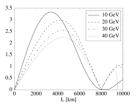
(a)	(b)

Figure 2: a) Scaling with $L$ of the ratio of the number of wrong-sign muons $\mu^{-}$ induced solely by $P_{2}$ in Eq. (19) to the statistical error in the total number of wrong-sign muons, for $\delta=0^{\circ}$; b) the same for wrong-sign muons $\mu^{-}$ induced by $P_{3}$, for $\delta=90^{\circ}$. The normalization of the $y$ axis is arbitrary. The oscillation parameters are: $\Delta m_{23}^{2}=2.8\times 10^{-3}$ eV², $\Delta m_{12}^{2}=1\times 10^{-4}$ eV², $\theta_{12}=22.5^{\circ}$, $\mbox{$\theta_{23}$}=45^{\circ}$ and $\mbox{$\theta_{13}$}=8^{\circ}$.

For $\mbox{$\theta_{13}$}\geq 1^{\circ}$, the dominant contributions in Eq. (18) are:

$$P_{1} \equiv s_{23}^{2}\sin^{2}2\mbox{$\theta_{13}$}\left(\frac{\mbox{$\Delta_{13}$}}{\tilde{B}_{\mp}}\right)^{2}\,\sin^{2}\left(\frac{\tilde{B}_{\mp}\,L}{2}\right)\,,$$

$$P_{2} \equiv \tilde{J}\;\frac{\Delta_{12}}{A}\frac{\mbox{$\Delta_{13}$}}{\tilde{B}_{\mp}}\,\cos\delta\cos\left(\frac{\mbox{$\Delta_{13}$}\,L}{2}\right)\;\sin\left(\frac{A\,L}{2}\right)\sin\left(\frac{\tilde{B}_{\mp}\,L}{2}\right)\,,$$

$$P_{3} \equiv \pm\tilde{J}\;\frac{\Delta_{12}}{A}\frac{\mbox{$\Delta_{13}$}}{\tilde{B}_{\mp}}\,\sin\delta\sin\left(\frac{\mbox{$\Delta_{13}$}\,L}{2}\right)\;\sin\left(\frac{A\,L}{2}\right)\sin\left(\frac{\tilde{B}_{\mp}\,L}{2}\right)\,.$$ (19)

In Fig. 2 we show the significance of the $\delta$-dependent terms, $P_{2}$ and $P_{3}$, as function of $L$. The significance is defined as the fraction of wrong-sign muons–for positive muons in the beam– resulting from a given term, over the statistical error in the measurement of the total number of wrong-sign muons. Results for several values of the neutrino energy are depicted.

The term in $\cos\delta$, $P_{2}$, is more significant than $P_{3}$ at short distances. Unfortunately, this sensitivity to $\delta$ through $P_{2}$ is fake, because at short distances there is no way to separate $P_{2}$ from the leading term, $P_{1}$: they have similar energy dependence and do not differ in the two polarities, as illustrated in Fig. 3. In order words, a change in $\delta$ can be compensated by a change in $\theta_{13}$ to keep the total probability unchanged.

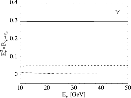
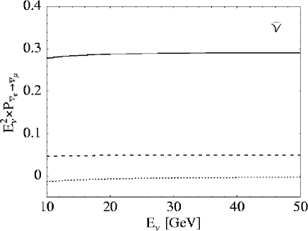
(a)	(b)

Figure 3: Neutrino energy dependence of the different terms in Eqs. (19): $E^{2}_{\nu}\,P_{1}$ (solid line), $E^{2}_{\nu}\,P_{2}$ $\delta=0^{\circ}$ (dashed line) for and $E^{2}_{\nu}\,P_{3}$ for $\delta=90^{\circ}$ (dotted line) , at $L=$ 732 km, for neutrinos (a) and antineutrinos (b). The parameters correspond to the LMA-MSW solution: $\Delta m_{23}^{2}=2.8\times 10^{-3}$ eV², $\Delta m_{12}^{2}=1\times 10^{-4}$ eV², $\theta_{12}=22.5^{\circ},\mbox{$\theta_{23}$}=45^{\circ}$ and $\mbox{$\theta_{13}$}=8^{\circ}$.

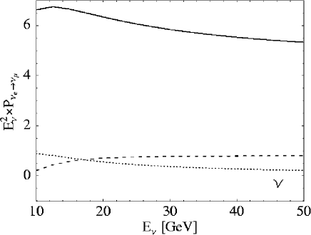
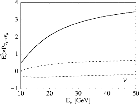
(a)	(b)

Figure 4: The same as in Fig. 3 but for $L=$ 3500 km.

At 3500 km the situation is very different, though: as Fig. 4 illustrates, the energy dependence of the three terms is quite different and furthermore $P_{3}$ –which changes sign with the beam polarity– is considerably larger. The comparison of the number of wrong-sign muons detected running in the two polarities and the binning in energy of the signal are thus strong analysis tools to disentangle $\theta_{13}$ and $\delta$ at baselines around 3500 km. Notice that this optimal distance is in nice agreement with the previous studies based on the significance of integrated asymmetries [18, 21, 41], updated in Fig. 5 for the present set-up.

The summary of this long discussion is that baselines much larger than 732 km are needed, for the following reasons:

• In the SMA-MSW or VO scenarios, the sign of $\Delta m^{2}_{23}$ can only be determined for distances such that matter effects are sizeable and the CP asymmetries they induce measurable. This happens at $L={\cal O}$ (3000 km) or larger.

• In the LMA-MSW scenario, there is a strong correlation between $\theta_{13}$ and $\delta$ at short distances. It is necessary to go far so that the terms most sensitive to them show a different energy dependence, and the signals in the CP-conjugate channels differ sizeably, allowing the simultaneous measurement of both parameters.

These expectations will be sustained by a detailed energy analysis in the following sections.

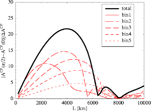
Figure 5: The signal-over-noise ratio of the CP-odd asymmetry of Eq. (12) as a function of the distance, after subtracting the fake matter induced asymmetry. The thick line corresponds to the integrated asymmetry, while the dashed lines correspond to the asymmetry computed in five energy bins of equal width $\Delta E_{\nu}=10$ GeV. The neutrino mixing parameters correspond to the LMA-MSW solution to the solar anomaly: $\Delta m_{23}^{2}=2.8\times 10^{-3}$ eV², $\Delta m_{12}^{2}=1\times 10^{-4}$ eV², $\theta_{12}=22.5^{\circ}$, $\mbox{$\theta_{23}$}=45^{\circ}$, $\mbox{$\theta_{13}$}=13^{\circ}$ and $\delta=90^{\circ}$. The muon energy is $E_{\mu}=$ 50 GeV and the matter parameter $A$ is varied with the distance as in [39].

4 Detection of wrong sign muons

4.1 A Large Magnetized Calorimeter

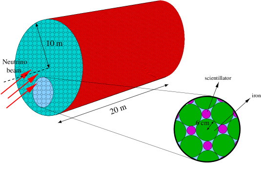
Figure 6: Sketch of the Large Calorimeter for the Neutrino Factory.

For the present study we consider a Large Magnetized Iron Calorimeter such as the one proposed in [29]. The apparatus, shown in Fig. 6 is a huge cylinder, of $10$ m radius and $20$ m length. It is made of $6$ cm thick iron rods intersped with $2$ cm thick scintillators segmented along their length. Its fiducial mass is $40$ kT. A superconducting coil generates a solenoidal magnetic field of 1 T.

The detector axis is oriented to form a few degrees with the direction of the neutrino beam. Thus, a neutrino crossing the detector sees a sandwich of iron and scintillator. The coordinates of the track transverse to the cylinder axis are measured from the location of the scintillator rods, while the longitudinal coordinate is measured from their segmentation. As discussed in [29], the performance of the device would be similar to the one expected for the MINOS detector [42].

Neutrino interactions in such a detector have a clear signature. For example, a $\nu_{\mu}$ charged current (CC) event is characterized by a muon, which is seen as a penetrating long track, plus a shower resulting from the interactions of the hadrons in the event. Fitting the muon track determines its charge and momentum, and a calorimetric measurement allows the determination of the hadronic momentum vector. In contrast, for a $\nu_{e}$ CC event the electromagnetic shower due to the prompt electron cannot be disentangled from the hadronic shower in an event-by-event basis, and therefore, the event looks similar to a neutral current (NC), which is characterized by having no penetrating track.

A realistic simulation of the response of an iron calorimeter must be able to compute: 1) whether the primary muon characterizing a CC event was identified or not, 2) whether non prompt muons arising from the decays of hadrons were missidentified as primary muons and 3) the muon and hadronic momentum vectors.

To address the above points we have written a Monte Carlo simulation based in the GEANT 3 package [43]. The apparatus is simulated with the correct geometry, and neutrino interactions are generated at random points in the fiducial volume. Then, every particle produced in the interaction is followed until it decays, exits the detector or undergoes a nuclear interaction.

When the muon track is very short, it cannot be disentangled from the other tracks in the hadronic jets. The peak of the hadron shower occurs at about 10 cm from the interaction vertex and essentially no hadronic activity remains at 100 cm from it. We thus impose the conservative criteria that, in order to be reconstructed, a muon track must be longer than 100 cm. About 99.2 % of all $\nu_{\mu}$ CC events at 50 GeV produce primary muons that satisfy this condition.

All muons, either primary or arising from the decay of hadrons, are tracked through the entire volume, and a hit is recorded each time a scintillator rod is crossed. The tracks can then be fitted to obtain the muon momentum. However, once the distance travelled by the muon is known, it is more efficient to use a simple smearing, which takes into account correctly both the effect of detector resolution and the multiple scattering.

As an illustration of the smearing procedure, the relative error in the measurement of the muon momentum as a function of the muon momentum is shown in Fig. 7. The resolution decreases rapidly for low momentum muons (for $P_{\mu}<5$ GeV, a much better resolution would be obtained from the measurement of the muon range), and improves rather smoothly for large momentum ($\delta P_{\mu}/P_{\mu}\sim 4\%$ for $P_{\mu}\sim 7~{}$GeV, while $\delta P_{\mu}/P_{\mu}\sim 3\%$ for $P_{\mu}\sim 50~{}$GeV). The fact that $\delta P_{\mu}/P_{\mu}$ is almost constant for large momentum is due to the dominance of the multiple scattering term in the resolution.

Hadrons, in contrast, are followed until they decay or undergo a nuclear interaction. In the latter case their momenta are added to the hadronic energy vector. Finally, both the magnitude and direction of the hadronic vector was smeared to account for the resolution of the detector. For details we refer to [29].

Figure 7: Relative error in the measurement of the muon momentum as a function of the muon momentum.

A large sample of neutrino interactions, corresponding to $10^{7}$ $\overline{\nu}_{\mu}$ charged and neutral currents, $5\times 10^{6}$ $\nu_{e}$ charged and neutral currents and the same data samples for the opposite polarity were analyzed for this study.

4.2 Search for wrong-sign muon events

We consider first the ($\overline{\nu}_{\mu}$ , $\nu_{e}$ ) neutrino beams originating from a $\mu^{+}$ beam of $E_{\mu}=50$ GeV (the dependence of the backgrounds with the energy of the muon beam was discussed in [29], where it was shown that optimal performance is obtained at the highest possible energy). The bulk of the events in the detector are $\overline{\nu}_{\mu}$ charged currents, signaled by the presence of a positive primary muon in the event, $\overline{\nu}_{\mu}$ and $\nu_{e}$ neutral currents, which are events with no primary leptons, and $\nu_{e}$ charged currents, for which we assume that the primary electron is not identified. On top of those events, one searches for wrong sign $\mu^{-}$ arising from the $\nu_{\mu}$ produced via the oscillation $\nu_{e}\rightarrow\nu_{\mu}$. Table 2 shows the number of interactions corresponding to a total of $10^{21}$ useful $\mu^{+}$ decays and a 40 kT detector at our reference baselines. For illustration, we will consider the oscillation parameters for the signal in the LMA-MSW scenario: $\Delta m^{2}_{23}=4\times 10^{-3}$eV², $\Delta m^{2}_{12}=10^{-4}$ eV², $\theta_{13}=13^{\circ}$, $\theta_{12}=22.5^{\circ}$ and $\theta_{23}=45^{\circ}$, as in the tables of Appendix B. Notice however that our results for the fractional background and efficiencies should be rather insensitive to the particular choice of parameters.

Baseline (km)	$\overline{\nu}_{\mu}$ CC	$\nu_{e}$ CC	$\overline{\nu}_{\mu}$ + $\nu_{e}$ NC	$\nu_{\mu}$(signal)
732	$3.5\times 10^{7}$	$5.9\times 10^{7}$	$3.1\times 10^{7}$	$1.1\times 10^{5}$
3500	$1.5\times 10^{6}$	$2.6\times 10^{6}$	$1.3\times 10^{6}$	$1.0\times 10^{5}$
7332	$3.5\times 10^{5}$	$5.9\times 10^{5}$	$3.0\times 10^{5}$	$3.8\times 10^{4}$

Table 2: Data samples expected in a 40 kT detector for $10^{21}$ useful $\mu^{+}$ decays. $\nu_{e}\rightarrow\nu_{\mu}$ oscillations with parameters as in Appendix B.

The potential backgrounds to the wrong sign $\mu^{-}$ events signaling the presence of oscillations are:

1. $\overline{\nu}_{\mu}$ CC events in which the positive muon is not detected, and a secondary negative muon arising from the decay of $\pi^{-},K^{-}$ and $D^{-}$ hadrons fakes the signal. The most dangerous events are those with $D^{-}\rightarrow\mu^{-}$, which yield an energetic muon with a spectrum similar to the signal.

2. $\nu_{e}$ CC events, for which it is assumed that the primary electron is never detected. Charm production is not relevant for this type of events since the charmed hadrons in the hadronic jet are predominantly positive. Instead, fake $\mu^{-}$ arise from the decay of negative pions and kaons in the hadronic jet.

3. $\overline{\nu}_{\mu}$ and $\nu_{e}$ NC events. Fake $\mu^{-}$ arise in this case also predominantly from the decay of negative pions and kaons, since charm production is suppressed with respect to the case of CC.

At first sight these backgrounds seem impressive. Fortunately, simple kinematical cuts can suppress them very efficiently. One exploits the fact that for signal events the $\mu^{-}$ candidate is harder and more isolated from the hadronic jet than for background events. We thus perform a simple analysis based in two variables, namely: the momentum of the muon, $P_{\mu}$, and a variable measuring the isolation of the muon, $Q_{t}=P_{\mu}\sin\theta$ (see Fig. 8).

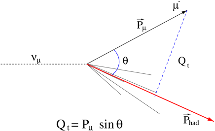
Figure 8: Definition of the kinematical variables used in this study.

To illustrate the rejection power of this analysis, Fig. 9 shows the efficiency for signal detection and the fractional backgrounds as a function of $P_{\mu}$ and $Q_{t}$ for $\overline{\nu}_{\mu}$ charged and neutral currents. Also shown is the signal-to-noise ratio, $S/N$, defined as the ratio of the signal selection efficiency and the error in the subtraction of the number of background events that pass the cuts, $N_{b}$. The error is taken to be Gaussian for large $N_{b}$ ($\sim\sqrt{N_{b}}$) and Poisson otherwise. Notice that charm production is the dominant background for $\overline{\nu}_{\mu}$ CC, while $\pi$ decay dominates the NC backgrounds.

$\overline{\nu}_{\mu}$Charged Currents

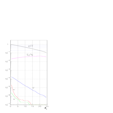
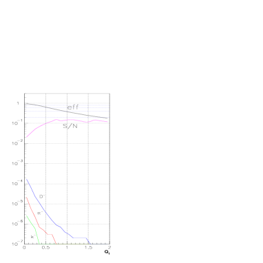
$\overline{\nu}_{\mu}$Neutral Currents

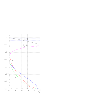
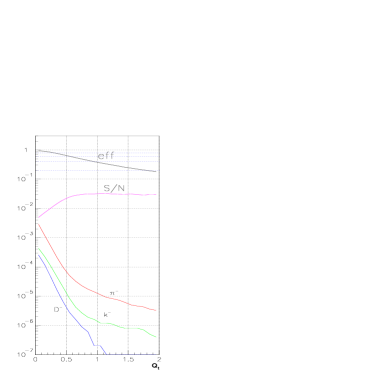
Figure 9: Signal and backgrounds for $\overline{\nu}_{\mu}$ CC and NC events.

Inspection of Fig. 9 shows that the $S/N$ is rather flat for $P_{\mu}>5~{}$GeV and $Q_{t}>0.5~{}$GeV. Cutting at $P_{\mu}>7.5~{}$GeV, $Q_{t}>1.0~{}$GeV, maximizes $S/N$. However, given the flatness of the $S/N$ ratio, one can vary these values generously with very little difference in the final results. Table 3 shows the fractional background contamination and the signal efficiency, while Table 4 shows the number of background and signal events that pass the cuts for the data sample discussed above. Notice that the residual backgrounds are quite sizeable at $L=732~{}$km, small at $L=3500~{}$km and negligible at $L=7332~{}$km. It is possible to optimize the analysis for very long baseline in order to achieve higher efficiency. However, we have chosen to use the same set of cuts for the three baselines.

$\overline{\nu}_{\mu}$ CC	$\nu_{e}$ CC	$\overline{\nu}_{\mu}$+ $\nu_{e}$NC	$\nu_{\mu}$(signal)
$1.0\times 10^{-7}$	$5.0\times 10^{-7}$	$1.0\times 10^{-6}$	$3\times 10^{-1}$

Table 3: Fractional backgrounds and signal selection efficiency for the wrong sign muon search with $\mu^{+}$ decays.

Baseline (km)	$\overline{\nu}_{\mu}$ CC	$\nu_{e}$ CC	$\overline{\nu}_{\mu}$+ $\nu_{e}$NC	$\nu_{\mu}$(signal)
732	$3.5$	$30$	$31$	$3.3\times 10^{4}$
3500	$0.1$	$1.2$	$1.2$	$3\times 10^{4}$
7332	$<0.1$	$<0.2$	$<0.2$	$1.3\times 10^{4}$

Table 4: Events surviving the cuts in a 40 kT detector for $10^{21}$ useful $\mu^{+}$ decays. Oscillation parameters as in Appendix B.

A potential source of fake wrong sign muons not discussed here is that due to a wrong measurement of the charge. In [29] it was estimated that, for $E_{\mu}=50~{}$GeV, this background could be reduced to a very small level, of the order of $10^{-6}$ or less. We have not included this source of background in the analysis.

The same exercise has to be repeated when a $\mu^{-}$ beam is considered. The resulting neutrino beams are now $\nu_{\mu}$ and $\overline{\nu}_{e}$ and the signal events are $\overline{\nu}_{\mu}$ . Fig. 10 shows the efficiency for signal detection and the fractional backgrounds, as a function of $P_{\mu}$ and $Q_{t}$, for $\nu_{\mu}$ charged and neutral currents. Tables 5, 6 and 7 summarize the results obtained (the cuts are the same than for the $\mu^{+}$ analysis). Finally, Fig. 11 shows the signal efficiency and the fractional backgrounds for $\mu^{+}$’s and $\mu^{-}$’s, as a function of the neutrino energy.

$\nu_{\mu}$Charged Currents

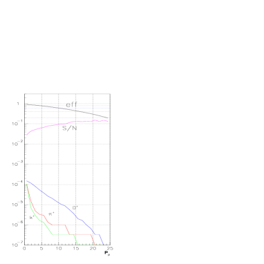
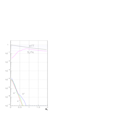
$\nu_{\mu}$Neutral Currents

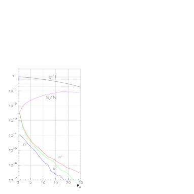
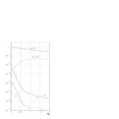
Figure 10: Signal and backgrounds for $\nu_{\mu}$ CC and NC events.

Baseline (km)	$\nu_{\mu}$ CC	$\overline{\nu}_{e}$ CC	$\nu_{\mu}$+ $\overline{\nu}_{e}$NC	$\overline{\nu}_{\mu}$ (signal)
732	$6.9\times 10^{7}$	$3.0\times 10^{7}$	$3.1\times 10^{7}$	$5\times 10^{4}$
3500	$3.0\times 10^{6}$	$1.3\times 10^{6}$	$1.4\times 10^{6}$	$1.6\times 10^{4}$
7332	$6.9\times 10^{5}$	$3.0\times 10^{5}$	$3.1\times 10^{5}$	$0.2\times 10^{4}$

Table 5: Data samples expected in a 40 kT detector for $10^{21}$ useful $\mu^{-}$ decays.

$\nu_{\mu}$ CC	$\overline{\nu}_{e}$ CC	$\nu_{\mu}$ + $\overline{\nu}_{e}$ NC	$\overline{\nu}_{\mu}$ (signal)
$3.0\times 10^{-7}$	$6.0\times 10^{-7}$	$2.0\times 10^{-6}$	$4.0\times 10^{-1}$

Table 6: Fractional backgrounds and signal selection efficiency for the wrong-sign muon search with $\mu^{-}$ decays.

Baseline (km)	$\nu_{\mu}$ CC	$\overline{\nu}_{e}$ CC	$\nu_{\mu}$ + $\overline{\nu}_{e}$ NC	$\overline{\nu}_{\mu}$ (signal)
732	$21$	$18$	$66$	$2.0\times 10^{4}$
3500	$0.9$	$0.8$	$2.4$	$6.4\times 10^{3}$
7332	$0.2$	$0.2$	$0.6$	$8.0\times 10^{2}$

Table 7: Events surviving the cuts in a 40 kT detector for $10^{21}$ useful $\mu^{-}$ decays.

In summary, our study shows that a large magnetized iron calorimeter allows the detection, with high efficiency ($\sim 30$–$40\%$) of the golden-plated wrong-sign muon signal. The different backgrounds to this signal can be efficiently controlled using simple cuts, which exploit the different kinematics between signal and background events. The charm background can be suppressed to circa $10^{-7}$, taking advantage of the high degree of collimation with the hadronic jet of charmed hadrons produced by 50 GeV muons. Instead, decays of energetic pions or kaons in NC events contaminate the signal at the $10^{-6}$ level. The optimization of the $S/N$ ratio points to the intermediate distances of $O(3500$) km as the optimal baseline.

5 Analysis in energy bins

A conservative estimate for the neutrino energy resolution in a detector of the type described in the previous section is $\Delta E_{\nu}/E_{\nu}\sim 20\%$. For a $\mu$ beam of 50 GeV and the statistics of oscillated neutrinos expected in the range of parameters considered, it is reasonable to bin the data in five bins of equal width $\Delta E_{\nu}=10$ GeV.

Let $N_{i,p}^{\lambda}$ be the total number of wrong-sign muons detected when the factory is run in polarity $p=\mu^{+},\mu^{-}$, grouped in 5 energy bins specified by $i=$ 1 to 5, and three possible distances, $\lambda=$ 1 (732 km), 2 (3500 km), 3 (7332 km).

In order to simulate a typical experimental situation we generate a set of “data” $n_{i,p}^{\lambda}$ as follows: for a given value of the oscillation parameters, the expected number of events, $N_{i,p}^{\lambda}$, is computed; taking into account backgrounds and detection efficiencies per bin, $b_{i,p}^{\lambda}$ and $\epsilon_{i,p}^{\lambda}$, as given in Fig. 11, we then perform a Gaussian (or Poisson, depending on the number of events) smearing to mimic the statistical uncertainty. All in all,

$$n_{i,p}^{\lambda}=\frac{{\rm Smear}(N_{i,p}^{\lambda}\epsilon_{i,p}^{\lambda}+b_{i,p}^{\lambda})-b_{i,p}^{\lambda}}{\epsilon_{i,p}^{\lambda}}\,.$$ (20)

Figure 11: Signal efficiency and total fractional backgrounds for the polarities $\mu^{+}$ (up) and $\mu^{-}$ (down) as a function of the neutrino energy.

The “data” are then fitted to the theoretical expectation as a function of the neutrino parameters under study, using a $\chi^{2}$ minimization,

$$\chi_{\lambda}^{2}=\sum_{p}\sum_{i}\left(\frac{n^{\lambda}_{i,p}\,-\,N^{\lambda}_{i,p}}{\delta n^{\lambda}_{i,p}}\right)^{2}\,,$$ (21)

where $\delta n^{\lambda}_{i,p}$ is the error of $n^{\lambda}_{i,p}$ (we include no error in the efficiencies). We perform and compare six different fits using: $\chi^{2}_{1}$, $\chi^{2}_{2}$, $\chi^{2}_{3}$ for the three distances, and the combinations $\chi^{2}_{1}\,+\,\chi^{2}_{2}$, $\chi^{2}_{2}\,+\,\chi^{2}_{3}$, $\chi^{2}_{1}\,+\,\chi^{2}_{2}\,+\,\chi^{2}_{3}$ to illustrate the gain in case the neutrino factory shoots to more than one location, a natural scenario given the ring configurations under study. For simplicity, we will consider a fit in at most two parameters at a time. All numerical results below will be obtained with the exact formulae for the oscillation probabilities.

6 SMA-MSW or Vacuum solar deficit

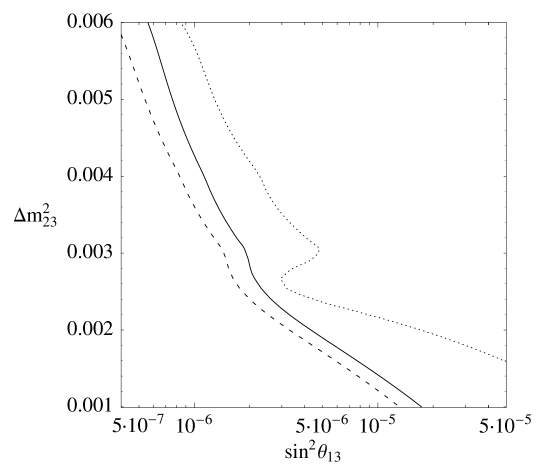
Figure 12: Asymptotic sensitivity to $\sin^{2}\mbox{$\theta_{13}$}$ as a function of $\Delta m^{2}_{23}$ at 90% CL for $L=732$ km (dashed lines), 3500 km (solid lines) and 7332 km (dotted lines), in the SMA-MSW solution. Only stastistical errors are included.

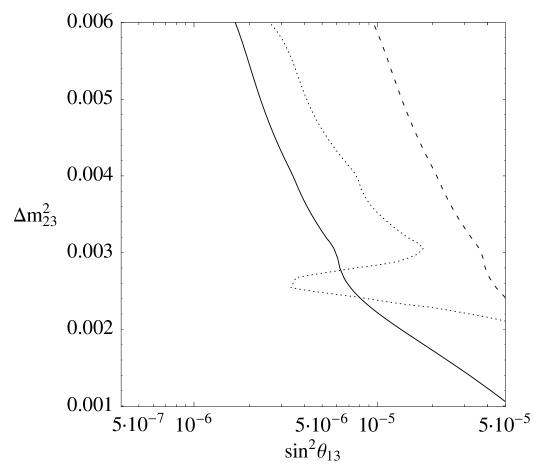
Figure 13: As in Fig. 12, including as well background errors and detection efficiencies.

For the SMA-MSW or VO scenarios, the influence of solar parameters on the neutrino factory signals will be negligible, and CP-violation out of reach. Besides its capability to reduce the errors on $\theta_{23}$ and $|\Delta m_{23}^{2}|$ to $\sim 1\%$ [24], the factory would still be a unique machine to constrain/measure $\theta_{13}$ [18] and the sign of $\Delta m^{2}_{23}$ [22, 23, 24].

Consider first $\theta_{13}$. In Fig. 12, we show the exclusion plot at 90% CL, on the $\Delta m^{2}_{23}$ (in the range allowed by SuperK) versus $\sin^{2}\mbox{$\theta_{13}$}$ plane, obtained with the full unbinned statistics and the two polarities. The same results, but including as well background errors and detection efficiencies are shown in Fig. 13. The statistical treatment in the presence of backgrounds is done as in [44]. Notice that the sensitivity is better at $L=$ 3500 km than at 732 km when efficiencies and backgrounds are included. The latter are responsible for it. The sensitivity at $7332$ km is also worse than at $3500$ km, due to the loss in statistics. In conclusion, the sensitivity to $\theta_{13}$ can be improved by three-four orders of magnitude with respect to the present limits. This is consistent with the results of [18] given the different statistics used.

The second major topic would be to perform the first precise measurements related to matter effects, in order to determine the sign of $\Delta m^{2}_{23}$ [24] and the size of the matter parameter, $A\propto n_{e}$.

We have studied the determination of the sign of $\Delta m^{2}_{23}$, assuming that the absolute value has by then been measured with a precision of 10%. We have explored the region around the best fit values of SuperKamiokande: $|\Delta m_{23}^{2}|=2.8\times 10^{-3}$ eV² and $\mbox{$\theta_{23}$}=45^{\circ}$. We perform a $\chi^{2}$ analysis on the $\Delta m^{2}_{23},\mbox{$\theta_{13}$}$ plane, as described in last section. The conclusion is that, for “data” generated within the range $\mbox{$\theta_{13}$}=1$–$10^{\circ}$ and $|\Delta m^{2}_{23}|$ in the range allowed by SuperKamiokande, a missidentification of the sign of $\Delta m^{2}_{23}$ can be excluded at 99% CL at 3500 km and 7332 km, but not at the shortest distance, 732 km. This conclusion agrees with the analysis of ref. [24], which did not include the energy dependence information.

We have further studied how the matter parameter of Eq. (14) and the angle $\theta_{13}$ can be measured simultaneously. Fig. 14 shows the result of a $\chi^{2}$ fit as described in section 5. Only statistical errors have been included in this figure. The corresponding results including as well background errors and detection efficiencies are shown in Fig. 15. At 732 km there is no sensitivity to the matter term, as expected. However, already at 3500 km, $A$ can be measured with a 10% precision. At the largest baseline, the precision in $A$ improves although at the expense of loosing precision in $\theta_{13}$ due to the loss in statistics. The level of precision discussed here might even be interesting for geophysicists [45].

Figure 14: 68.5, 90, 99 % CL resulting from a simultaneous fit of $\theta_{13}$ and $A$. The parameters used to generate the “data” are denoted by a star, while the baseline(s) used in the fit is indicated in each plot. Only statistical errors included.

Figure 15: The same as in Fig. 14 but including backgrounds and efficiencies.

The above conclusions also hold for the vacuum solution to the solar deficit.

7 LMA-MSW

Assume now the LMA-MSW scenario. Fixed values of the atmospheric parameters are used in this section, $\Delta m_{23}^{2}=2.8\times 10^{-3}$ eV² and maximal mixing, $\mbox{$\theta_{23}$}=45^{\circ}$. A precision of $1\%$ in these parameters is achievable through muon disappearance measurements at the neutrino factory [24]. This level of uncertainty is not expected to affect the results of this section.

Let us start discussing the measurement of the CP phase $\delta$ versus $\theta_{13}$. We have studied numerically how to disentangle them in the range $1$–$10^{\circ}$ and $0\leq\delta\leq 180^{\circ}$.

Consider first the upper solar mass range allowed by the LMA-MSW solution: $\Delta m_{12}^{2}=10^{-4}$ eV². Fig. 16 shows the confidence level contours for a simultaneous fit of $\theta_{13}$ and $\delta$, for “data” corresponding to $\mbox{$\theta_{13}$}=8^{\circ}$, $\delta=54^{\circ}$, including only statistical errors in the analysis. Fig. 17 shows the same analysis taking into account the background errors and detection efficiencies of Fig. 11. The correlation between $\delta$ and $\theta_{13}$ is very large at the shortest baseline 732 km, as argued in section 3. The phase $\delta$ is then not measurable and this indetermination induces a rather large error on the angle $\theta_{13}$. However, at the intermediate baseline of 3500 km the two parameters can be disentangled and measured. At the largest baseline, the sensitivity to $\delta$ is lost and the precision in $\theta_{13}$ becomes worse due to the smaller statistics. The combination of the results for 3500 km with that for any one of the other distances improves the fit, but not in a dramatic way. Just one detector placed at ${\cal O}$ (3000 km) may be sufficient: a precision of few tenths of degree is attained for $\theta_{13}$ and of a few tens of degrees for $\delta$.

Figure 16: 68.5, 90, 99 % CL contours resulting from a $\chi^{2}$ fit of $\theta_{13}$ and $\delta$. The parameters used to generate the “data” are depicted by a star and the baseline(s) which is used for the fit indicated in each plot. Only statistical errors are included.

Figure 17: The same as Fig. 16 with backgrounds and efficiencies included.

Similar figures are obtained for “data” corresponding to smaller values of $\theta_{13}$, as shown in Fig. 18 for $\mbox{$\theta_{13}$}=2^{\circ}$. The pattern is maintained as well for different values of $\delta$: see Fig. 19 for “data” corresponding to $\delta=0^{\circ}$ and $\mbox{$\theta_{13}$}=8^{\circ}$. This last figure also proves that, if the sign of $\Delta m_{12}^{2}$ is known by the time the neutrino factory will be operative, $\delta=0^{\circ}$ is distinguishable from $\delta=180^{\circ}$ with just one baseline. This exemplifies the power of the analysis of the energy dependence. Recall in any case that a $\pi$-ambiguity on $\delta$ has no bearing on the existence of CP-violation, and we will go on considering positive values of $\Delta m_{12}^{2}$.

Figure 18: As Fig. (17) for different values of the parameters denoted by the star.

Figure 19: As Fig. (17) for different values of the parameters denoted by the star.

The sensitivity to CP-violation decreases linearly with $\Delta m_{12}^{2}$. At the central value allowed by the LMA-MSW solution, $\Delta m_{12}^{2}=5\times 10^{-5}$ eV², CP-violation can still be discovered, as shown in Fig. 20. At the lower value allowed, $\Delta m_{12}^{2}=1\times 10^{-5}$ eV², the sensitivity to CP-violation is lost with the experimental set-up considered, as shown in Fig. 21.

Figure 20: Fit for $\Delta m_{12}^{2}=5\times 10^{-5}$ eV² including backgrounds errors and detection efficiencies. The star indicates the parameters used to generate the “data”.

Figure 21: As Fig. 20, for $\Delta m_{12}^{2}=1\times 10^{-5}$ eV².

We have quantified what is the minimum value of $\Delta m^{2}_{12}$ for which a maximal CP-odd phase, $\delta=90^{\circ}$, can be distinguished at 99% CL from $\delta=0^{\circ}$. The result is shown in Fig. 22: $\Delta m^{2}_{12}>2\times 10^{-5}$ eV², with very small dependence on $\theta_{13}$, in the range considered.

Figure 22: Lower limit in $\Delta m_{12}^{2}$ at which a maximal CP phase ($90^{\circ}$) can be distinguished from a vanishing phase at 99% CL, as a function of $\theta_{13}$ at $L=$ 3500 km. Background errors and efficiencies are included.

One word of caution is pertinent: up to now we assumed $|\Delta m^{2}_{12}|$ and $\sin 2\theta_{12}$ known by the time the neutrino factory will be operational. Otherwise, the correlation of these parameters with $\theta_{13}$ would be even more problematic than that between $\delta$ and $\theta_{13}$, as illustrated in Fig. 23 for $|\Delta m^{2}_{12}|$. The error induced on the measurement of $\theta_{13}$ by the present uncertainty in $|\Delta m^{2}_{12}|$ is much larger than that stemming from the uncertainty on $\delta$. Fortunately, LBL reactor experiments will measure $|\Delta m^{2}_{12}|$ and $\sin 2\theta_{12}$ if it lies in the LMA-MSW range. Even if the error in these measurements is as large as 50%, the problem would be much less serious. We have checked that such uncertainty does not affect our results concerning the sensitivity to $\delta$, and only induces an error in $\theta_{13}$ that can be read from Fig. 23.

Figure 23: Simultaneous fit to $\theta_{13}$ and $\Delta m_{12}^{2}$. The range shown in the vertical axis is the presently allowed LMA-MSW range. The star indicates the parameters used to generate the “data” and the CP-odd phase is set to zero. Backgrounds and detection efficiencies are included.

Concerning the measurement of the matter parameter, we have considered simultaneous fits of $\theta_{13}$ and $A$, for two values of the CP-phase: $\delta=0,\pi/2$. The confidence level contours obtained are very similar to those in Fig. 14 for the SMA-MSW solution. This indicates that there is no dangerous correlation between $A$ and $\theta_{13}$ in the presence of sizeable $\delta$-dependent terms, and both parameters can be safely measured at 3500 km. However, it is important to stress that the simultaneous measurement of the three parameters $\theta_{13},\delta$ and $A$ will increase the errors with respect to the two-parameter fits performed here. In this respect the combination of two baselines: ${\cal O}$(3500 km) and ${\cal O}$(7332 km) may be helpful.

8 Summary

The neutrino beams obtained from muon storage rings will be excellent for precision neutrino physics. The appearance of wrong-sign muons is a powerful neutrino oscillation signal, which allows to improve considerably our knowledge of the leptonic flavour sector.

Two very important questions are the optimal energy for the decaying muons and the optimal detection distance(s), in view of the physics goals. The higher the parent muon energy, the larger the oscillation signals. This fact, together with the requirement of low backgrounds and good detection efficiencies, lead to consider muon energies as high as possible within realistic machine designs. Energies of a several tens of GeV are currently under discussion, assumed here to be $E_{\mu}=$ 50 GeV, for definiteness.

Energy and detection distance are intertwined in the oscillation pattern of neutrinos propagating in matter. We have derived an analytical approximate formula for the oscillation probabilities in matter, which helps to understand how the sensitivity to the most interesting quantities scales with the neutrino energy and distance.

We have shown that an analysis in neutrino energy bins, combined with a comparison of the signals obtained with the two polarities, allows to disentangle the unknown parameters at long enough baselines. In particular, for the LMA-MSW solution, $\theta_{13}$ and $\delta$ can be simultaneously measured. We have also studied realistic backgrounds and detection efficiencies. The overall conclusion is that the intermediate baseline of ${\cal O}$(3000 km) is optimal for the physics goals considered in this paper (see Fig. 24 for an artistic view of possible locations).

Quantitatively, our two parameter fits at 3500 km indicate:

• The angle $\theta_{13}$ can be measured with a precision of tenths of degrees, down to values of $\mbox{$\theta_{13}$}=1^{\circ}$. The asymptotic sensitivity to $\sin^{2}\mbox{$\theta_{13}$}$ can be improved by three orders of magnitude or more.

• If the solar deficit corresponds to solar parameters in the LMA-MSW range, CP-violation may be tackled. The phase $\delta$ can be determined with a precision of tens of degrees, for the central values allowed for $|\Delta m_{12}^{2}|$, and maximal CP-violation can be disentangled from no CP-violation at 99% CL for values of $|\Delta m_{12}^{2}|>2\times 10^{-5}$ eV².

• The sign of the atmospheric mass difference, $\Delta m_{23}^{2}$, can be determined at 99% CL, for $\theta_{13}$ within the range $\mbox{$\theta_{13}$}=1$–$10^{\circ}$ and $|\Delta m_{23}^{2}|$ in the range allowed by SuperKamiokande data.

• A model independent confirmation of the MSW effect will be feasible, and the matter parameter $A$ measured within a 10% precision, or better if combined with the longest baseline: $7332$ km.

In the case of the LMA-MSW solution, the combination of the two longest baselines may be useful if a multiparameter fit becomes necessary.

Even though non-zero neutrino masses are barely established, the neutrino sector of the theory can be convincingly argued to herald physics well beyond the standard model. It is in this perspective that a neutrino factory should be built.

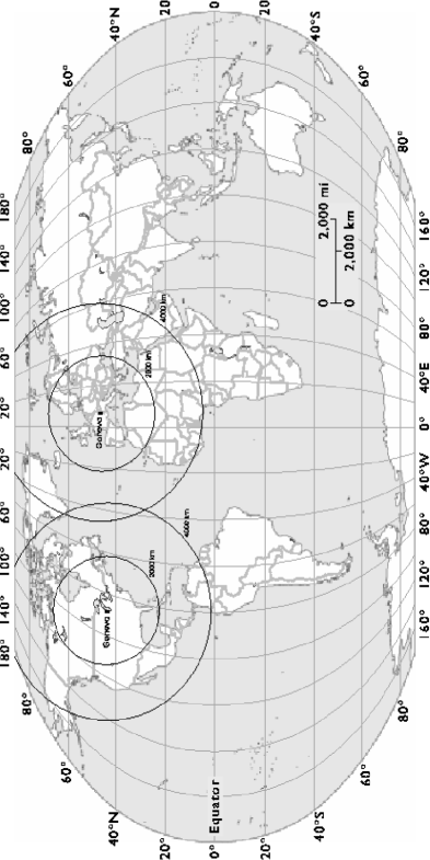
Figure 24: Artistic view of possible baselines of ${\cal O}$(3000 km) at which a neutrino factory, located at Geneva (Switzerland) or Geneva (Illinois), could shoot. The inner and outer circles correspond to 2000 and 4000 km, respectively. Note that the circles have not been projected onto the Earth surface.

9 Acknowledgements

We acknowledge useful conversations with: J. Bernabeu, A. de Gouvea, A. De Rújula, F. Dydak, J. Ellis and C. Quigg. We further thank A. De Rújula for suggestions and a critical reading of the manuscript. We thank P. Lipari for pointing out an incorrect statement in an earlier version of this paper. A. D. acknowledges the I.N.F.N. for financial support. S. R. acknowledges the European Union for financial support through contract ERBFMBICT972474. The work of A. D., M. B. G. and S. R. was also partially supported by CICYT project AEN/97/1678.

Appendix A: Non-oscillated statistics

Tab. 8 contains the results for the $\nu_{e}$ and $\bar{\nu}_{\mu}$ fluxes for the parent muon energy $E_{\mu}=$ 50 GeV and for $n_{\mu}=2\times 10^{20}$ useful muons per year, per 5 operational years. The result for three muon polarizations are shown: ${\cal P}_{\mu^{\pm}}=$ 0, $\mp$ 0.3 (the “natural” polarization) and $\mp 1$. For ${\cal P}_{\mu^{\pm}}=0$ our results agree with [26] when the same number of useful muons is considered.

For a $\mu^{+}$ ($\mu^{-}$) beam of $E_{\mu}=50$ GeV, the average neutrino and antineutrino energies are, for ${\cal P}_{\mu^{+}(\mu^{-})}=0$, $\langle E_{\bar{\nu}_{\mu}(\nu_{\mu})}\rangle=$ 35 GeV, and $\langle E_{\nu_{e}(\bar{\nu}_{e})}\rangle=$ 30 GeV. For ${\cal P}_{\mu^{+}(\mu^{-})}=-1(+1)$, we get $\langle E_{\bar{\nu}_{\mu}(\nu_{\mu})}\rangle=$ 30 GeV, $\langle E_{\nu_{e}(\bar{\nu}_{e})}\rangle=$ 30 GeV.

$E_{\mu^{\mp}}=50$ GeV		$\mu^{-}$		$\mu^{+}$
L (km)		$\Phi_{\nu_{\mu}}/10^{12}$	$\Phi_{\bar{\nu}_{e}}/10^{12}$	$\Phi_{\bar{\nu}_{\mu}}/10^{12}$	$\Phi_{\nu_{e}}/10^{12}$
732
	$0$	$123$	$122$	$123$	$122$
$\cal{P}_{\mu^{\mp}}$	${\pm}0.3$	$110$	$159$	$110$	$159$
	${\pm}1$	$81.5$	$244$	$81.5$	$244$
3500
	$0$	$5.35$	$5.35$	$5.35$	$5.35$
$\cal{P}_{\mu^{\mp}}$	${\pm}0.3$	$4.83$	$6.95$	$4.83$	$6.95$
	${\pm}1$	$3.56$	$10.7$	$3.56$	$10.7$
7332
	$0$	$1.22$	$1.22$	$1.22$	$1.22$
$\cal{P}_{\mu^{\mp}}$	${\pm}0.3$	$1.10$	$1.58$	$1.10$	$1.58$
	${\pm}1$	$0.81$	$2.43$	$0.81$	$2.43$

Table 8: Neutrino and antineutrino fluxes for L = 732, 3500 and 7332 Km per m² per 5 operational years when $2\times 10^{20}$ muons decay in the straight section of the storage ring. This fluxes have been averaged over an angular divergence of 0.1 mr.

$E_{\mu^{\mp}}=50$ GeV		$\mu^{-}$		$\mu^{+}$
L (km)		$N_{\nu_{\mu}}/10^{5}$	$N_{\bar{\nu}_{e}}/10^{5}$	$N_{\bar{\nu}_{\mu}}/10^{5}$	$N_{\nu_{e}}/10^{5}$
732
	$0$	$692$	$300$	$352$	$590$
$\cal{P}_{\mu^{\mp}}$	${\pm}0.3$	$603$	$390$	$306$	$768$
	${\pm}1$	$394$	$600$	$200$	$1180$
3500
	$0$	$30.4$	$13.1$	$15.4$	$25.8$
$\cal{P}_{\mu^{\mp}}$	${\pm}0.3$	$26.4$	$17.1$	$13.4$	$33.6$
	${\pm}1$	$17.2$	$26.2$	$8.75$	$51.6$
7332
	$0$	$6.90$	$3.00$	$3.50$	$5.88$
$\cal{P}_{\mu^{\mp}}$	${\pm}0.3$	$6.01$	$3.88$	$3.05$	$7.66$
	${\pm}1$	$3.92$	$5.98$	$1.99$	$11.8$

Table 9: Neutrino and antineutrino charged currents interaction rates for L = 732, 3500 and 7332 km per 40 kT and per 5 operational years when $2\times 10^{20}$ muons decay in the straight section of the storage ring. These fluxes have been averaged over an angular divergence of 0.1 mr.

Tab. 9 contains the numerical results for the number of CC interaction rates for $e^{\pm}$ and $\mu^{\mp}$ fluxes in a $\mu^{\mp}$ beam in a 40 kT detector with $n_{\mu}=2\times 10^{20}$ useful muons per year per 5 operational years. These results represent the number of leptons of a given flavour observed at the detector in case no neutrino oscillation occurs, neglecting detection efficiencies.

Appendix B: Oscillated statistics

As an illustration, we give the oscillated fluxes for three values of the atmospheric mass difference, $\Delta m^{2}_{23}=2,\,4,\,6\times 10^{-3}$ eV². The rest of the leptonic parameters are $\Delta m^{2}_{12}=10^{-4}$ eV², $\mbox{$\theta_{23}$}=45^{\circ}$, $\mbox{$\theta_{13}$}=13^{\circ}$ and $\theta_{12}=22.5^{\circ}$. The matter parameter is taken to be $A=1.1\times 10^{-4}$ eV${}^{2}/$GeV for the baselines of $L=$ 732 km and $L=$ 3500 km, while $A=1.5\times 10^{-4}$ eV${}^{2}/$GeV for $L=$ 7332 km. The in principle measurable quantities are the number of leptons of a given flavour and charge reaching the detector at a given baseline.

Tab. 10 shows the total number of leptons of different flavours ($\bar{\nu}_{e}\rightarrow\bar{\nu}_{\mu}\rightarrow\mu^{+}$,$\nu_{\mu}\rightarrow\nu_{e}\rightarrow e^{-}$, $\bar{\nu}_{e}\rightarrow\bar{\nu}_{\tau}\rightarrow\tau^{+}$ and $\nu_{\mu}\rightarrow\nu_{\tau}\rightarrow\tau^{-}$ for a $\mu^{-}$ beam) at 732 km. Tab. 11 shows the analogous results from $\mu^{+}$ decays. Detection efficiencies are not included. The whole exercise is repeated for the baselines $L=$ 3500 km and $L=$ 7332 km in Tabs. 12, 13 and 14, 15, respectively.

$\cal{P}_{\mu^{-}}$	$\Delta m_{23}^{2}$	$N_{\mu^{-}}/10^{5}$	$N_{e^{+}}/10^{5}$	$N_{\mu^{+}}/10^{3}$	$N_{e^{-}}/10^{3}$	$N_{\tau^{+}}/10^{3}$	$N_{\tau^{-}}/10^{4}$
	0.002	691	300	13.8	24.1	14.3	20.6
$0$	0.004	684	299	51.3	91.7	52.9	80.9
	0.006	673	298	110	201	113	178
	0.002	601	390	18.0	22.0	18.6	19.4
$0.3$	0.004	595	389	66.7	83.8	68.8	76.1
	0.006	584	387	143	184	147	167
	0.002	391	600	27.7	18.6	28.6	16.5
$1$	0.004	387	598	103	70.8	106	64.2
	0.006	378	596	220	155	226	140

Table 10: Calculated charged currents event rates for $\mu^{-}$ beam assuming neutrino oscillations in a 40 kT detector, for a L = 732 km baseline as a function of $E_{\mu}$, $\Delta m_{23}^{2}$, for different polarizations of the parent muon. We have considered $1\times 10^{21}$ negative muons decays ($2\times 10^{20}$ useful muons/year $\times$ 5 operational years).

$\cal{P}_{\mu^{+}}$	$\Delta m_{23}^{2}$	$N_{\mu^{+}}/10^{5}$	$N_{e^{-}}/10^{5}$	$N_{\mu^{-}}/10^{3}$	$N_{e^{+}}/10^{3}$	$N_{\tau^{-}}/10^{3}$	$N_{\tau^{+}}/10^{4}$
	0.002	351	590	28.9	11.7	28.0	10.5
$0$	0.004	348	588	110	43.6	106	41.4
	0.006	342	586	239	94.1	232	91.5
	0.002	305	767	37.5	11.2	36.4	9.86
$-0.3$	0.004	302	765	142	41.9	138	38.7
	0.006	297	762	311	90.1	302	85.4
	0.002	200	1180	57.8	9.52	56.0	8.36
$-1$	0.004	196	1170	219	35.2	212	32.7
	0.006	192	1172	478	75.3	464	71.6

Table 11: Calculated charged currents event rates for $\mu^{+}$ beam assuming neutrino oscillations in a 40 kT detector, for a L = 732 km baseline as a function of $E_{\mu}$, $\Delta m_{23}^{2}$, for different polarizations of the parent muon. We have considered $1\times 10^{21}$ positive muons decays ($2\times 10^{20}$ useful muons/year $\times$ 5 operational years).

$\cal{P}_{\mu^{-}}$	$\Delta m_{23}^{2}$	$N_{\mu^{-}}/10^{4}$	$N_{e^{+}}/10^{4}$	$N_{\mu^{+}}/10^{2}$	$N_{e^{-}}/10^{3}$	$N_{\tau^{+}}/10^{2}$	$N_{\tau^{-}}/10^{3}$
	0.002	282	130	65.8	21.1	75.3	187
$0$	0.004	232	128	163	81.9	187	631
	0.006	170	126	227	174	259	1150
	0.002	244	169	85.5	17.9	97.9	176
$0.3$	0.004	198	166	212	70.5	243	585
	0.006	143	164	295	150	337	1054
	0.002	156	260	132	15.3	151	145
$1$	0.004	120	256	327	58.7	373	463
	0.006	81.0	253	454	121	518	792

Table 12: Calculated charged currents event rates for $\mu^{-}$ beam assuming neutrino oscillations in a 40 kT detector, for a L = 3500 km baseline as a function of $E_{\mu}$, $\Delta m_{23}^{2}$, for different polarizations of the parent muon. We have considered $1\times 10^{21}$ negative muons decays ($2\times 10^{20}$ useful muons/year $\times$ 5 operational years).

$\cal{P}_{\mu^{+}}$	$\Delta m_{23}^{2}$	$N_{\mu^{+}}/10^{4}$	$N_{e^{-}}/10^{4}$	$N_{\mu^{-}}/10^{3}$	$N_{e^{+}}/10^{2}$	$N_{\tau^{-}}/10^{3}$	$N_{\tau^{+}}/10^{3}$
	0.002	143	254	25.7	60.4	22.9	100
$0$	0.004	118	240	96.4	164	88.1	348
	0.006	86.0	221	195	249	181	655
	0.002	124	330	33.4	62.4	29.8	92.7
$-0.3$	0.004	100	312	125	165	115	319
	0.006	72.4	287	254	246	235	592
	0.002	79.3	507	51.4	50.2	45.8	77.0
$-1$	0.004	60.8	480	193	124	176	254
	0.006	40.8	441	390	173	362	450

Table 13: Calculated charged currents event rates for $\mu^{+}$ beam assuming neutrino oscillations in a 40 kT detector, for a L = 3500 km baseline as a function of $E_{\mu}$, $\Delta m_{23}^{2}$, for different polarizations of the parent muon. We have considered $1\times 10^{21}$ positive muons decays ($2\times 10^{20}$ useful muons/year $\times$ 5 operational years).

$\cal{P}_{\mu^{-}}$	$\Delta m_{23}^{2}$	$N_{\mu^{-}}/10^{3}$	$N_{e^{+}}/10^{3}$	$N_{\mu^{+}}/10^{2}$	$N_{e^{-}}/10^{3}$	$N_{\tau^{+}}/10^{2}$	$N_{\tau^{-}}/10^{3}$
	0.002	527	299	2.38	3.97	1.94	159
$0$	0.004	256	296	16.7	28.2	15.1	406
	0.006	89.1	292	35.8	78.8	33.5	523
	0.002	451	388	3.10	3.95	2.52	146
$0.3$	0.004	212	385	21.6	27.3	19.6	362
	0.006	75.1	380	46.6	74.1	43.6	452
	0.002	273	597	4.77	3.89	3.88	115
$1$	0.004	110	592	33.3	25.2	30.1	257
	0.006	42.5	584	71.6	63.3	67.0	287

Table 14: Calculated charged currents event rates for $\mu^{-}$ beam assuming neutrino oscillations in a 40 kT detector, for a L = 7332 km baseline as a function of $E_{\mu}$, $\Delta m_{23}^{2}$, for different polarizations of the parent muon. We have considered $1\times 10^{21}$ negative muons decays ($2\times 10^{20}$ useful muons/year $\times$ 5 operational years).

$\cal{P}_{\mu^{+}}$	$\Delta m_{23}^{2}$	$N_{\mu^{+}}/10^{3}$	$N_{e^{-}}/10^{3}$	$N_{\mu^{-}}/10^{3}$	$N_{e^{+}}/10^{2}$	$N_{\tau^{-}}/10^{3}$	$N_{\tau^{+}}/10^{3}$
	0.002	265	577	6.06	1.16	5.84	85.6
$0$	0.004	125	513	38.1	11.5	37.8	225
	0.006	52.8	399	94.8	31.2	95.0	295
	0.002	227	750	7.88	1.20	7.59	78.6
$-0.3$	0.004	104	667	49.5	11.0	49.1	201
	0.006	47.6	519	123	28.5	123	255
	0.002	137	1150	12.1	129	11.7	62.4
$-1$	0.004	54.8	1030	76.2	10.0	75.6	144
	0.006	35.7	798	190	22.3	190	161

Table 15: Calculated charged currents event rates for $\mu^{+}$ beam assuming neutrino oscillations in a 40 kT detector, for a L = 7332 km baseline as a function of $E_{\mu}$, $\Delta m_{23}^{2}$, for different polarizations of the parent muon. We have considered $1\times 10^{21}$ positive muons decays ($2\times 10^{20}$ useful muons/year $\times$ 5 operational years).

Appendix C: Perturbative Expansion of Oscillation Probabilities

In this Appendix, we describe the perturbative expansion we have performed to obtain Eq. (18). The problem is to diagonalize the neutrino mass matrix,

$$M\equiv U\left(\matrix{0&0&0\cr 0&\Delta_{12}&0\cr 0&0&\mbox{$\Delta_{13}$}\cr}\right)U^{\dagger}+\left(\matrix{A&0&0\cr 0&0&0\cr 0&0&0\cr}\right)\,,$$ (22)

with $U$ as given in Eq. (1). The exact diagonalization of this matrix has been done in [40]. Since we are interested only in the case in which $\Delta m^{2}_{12}$ is small, it is adequate to use perturbation theory to compute corrections to first order in this quantity. This leads to much simpler analytical formulae.

In the limit $\Delta m^{2}_{12}=0$, the diagonalization of this matrix is very simple [38],

$$M_{\mp}^{(0)}\equiv\bar{U}_{\mp}\left(\matrix{\frac{\Delta_{13}\pm A-B_{\mp}}{2}&0&0\cr 0&0&0\cr 0&0&\frac{\Delta_{13}\pm A+B_{\mp}}{2}\cr}\right)\bar{U}_{\mp}^{\dagger}\,.$$ (23)

The matrix of eigenvectors is

$$\bar{U}_{\mp}\equiv U_{23}(\mbox{$\theta_{23}$})U_{13}(\theta_{M_{\mp}})\,,$$ (24)

where $\theta_{M_{\mp}}$ is defined by:

$$\tan 2\theta_{M_{\mp}}\equiv\frac{\mbox{$\Delta_{13}$}\sin 2\mbox{$\theta_{13}$}}{\mbox{$\Delta_{13}$}\cos 2\mbox{$\theta_{13}$}\mp A}\,.$$ (25)

$\theta_{M_{\mp}}$ is to be taken in the first (second) quadrant if $\mbox{$\Delta_{13}$}\,\cos 2\mbox{$\theta_{13}$}\mp A$ is positive (negative).

At first order in $\Delta_{12}$, the perturbation to Eq. (23) (in the basis of non-perturbated eigenvectors) is:

$$M_{\mp}^{(1)}\equiv\bar{U}_{\mp}^{\dagger}U\left(\matrix{0&0&0\cr 0&\Delta_{12}&0\cr 0&0&0\cr}\right)U^{\dagger}\bar{U}_{\mp}.$$ (26)

The eigenvalues at first order in $\Delta_{12}$ are:

$$\lambda^{(1)}_{1} = \lambda^{(0)}_{1}+s^{2}_{12}\Delta_{12}\cos^{2}\bar{\theta}_{M_{\mp}}\,,$$

$$\lambda^{(1)}_{2} = \lambda^{(0)}_{2}+c^{2}_{12}\Delta_{12}\,,$$

$$\lambda^{(1)}_{3} = \lambda^{(0)}_{3}+s^{2}_{12}\Delta_{12}\sin^{2}\bar{\theta}_{M_{\mp}}\,,$$ (27)

The corresponding (not normalized) eigenvectors are,

$$v^{(1)}_{1} = \left(1,\ \frac{\sin 2\theta_{12}\cos\bar{\theta}_{M_{\mp}}\Delta_{12}}{\mbox{$\Delta_{13}$}+A-B_{\mp}},\ \frac{s^{2}_{12}\Delta_{12}\sin\bar{\theta}_{M_{\mp}}e^{\mp i\delta}}{2B_{\mp}}\right)\,,$$

$$v^{(1)}_{2} = \left(\frac{\sin 2\theta_{12}\cos\bar{\theta}_{M_{\mp}}\Delta_{12}}{-\mbox{$\Delta_{13}$}-A+B_{\mp}},\ 1,\ \frac{\sin 2\theta_{12}\sin\bar{\theta}_{M_{\mp}}e^{\mp i\delta}\Delta_{12}}{\mbox{$\Delta_{13}$}+A+B_{\mp}}\right)\,,$$

$$v^{(1)}_{3} = \left(\frac{-s^{2}_{12}\sin 2\bar{\theta}_{M_{\mp}}\Delta_{12}e^{\pm i\delta}}{2B_{\mp}},\ \frac{-\sin 2\theta_{12}\sin\bar{\theta}_{M_{\mp}}\Delta_{12}e^{\pm i\delta}}{\Delta_{31}+A+B_{\mp}},\ 1\right),\,$$ (28)

where $\bar{\theta}_{M_{\mp}}\equiv\mbox{$\theta_{13}$}-\theta_{M_{\mp}}$.

With these results, it is easy to compute the oscillation probabilities, keeping consistently terms up to first order in $\Delta_{12}$. We obtain:

$$P_{\nu_{e}\nu_{\mu}(\bar{\nu}_{e}\bar{\nu}_{\mu})}=s^{2}_{23}\sin^{2}(2\theta_{M_{\mp}})\sin^{2}\left(\frac{B_{\mp}\,L}{2}\right)-$$

$$s^{2}_{23}s^{2}_{12}\left[\sin(4\theta_{M_{\mp}})\sin(2\bar{\theta}_{M_{\mp}})\sin^{2}\left(\frac{B_{\mp}\,L}{2}\right)\frac{\Delta_{12}}{B_{\mp}}+\sin^{2}(2\theta_{M_{\mp}})\cos(2\bar{\theta}_{M_{\mp}})\sin(B_{\mp}\,L)\frac{\Delta_{12}\,L}{2}\right]+$$

$$\sin(2\theta_{12})\sin(2\mbox{$\theta_{23}$})\sin(2\theta_{M_{\mp}})\sin\left(\frac{B_{\mp}\,L}{2}\right)\Delta_{12}\times$$

$$\left[\sin\left(\frac{\lambda^{(0)}_{1}\,L}{2}\right)\cos\left(\pm\delta-\frac{\lambda^{(0)}_{3}\,L}{2}\right)\left(\frac{\cos\theta_{M_{\mp}}\cos\bar{\theta}_{M_{\mp}}}{\lambda^{(0)}_{1}}-\frac{\sin\theta_{M_{\mp}}\sin\bar{\theta}_{M_{\mp}}}{\lambda^{(0)}_{3}}\right)-\right.$$

$$\left.\sin\theta_{M_{\mp}}\sin\bar{\theta}_{M_{\mp}}\cos\delta\sin\left(\frac{B_{\mp}\,L}{2}\right)\frac{1}{\lambda^{(0)}_{3}}\right]\,,$$ (29)

$$P_{\nu_{e}\nu_{\tau}(\bar{\nu}_{e}\bar{\nu}_{\tau})}=c^{2}_{23}\sin^{2}(2\theta_{M_{\mp}})\sin^{2}\left(\frac{B_{\mp}\,L}{2}\right)-$$

$$c^{2}_{23}s^{2}_{12}\left[\sin(4\theta_{M_{\mp}})\sin(2\bar{\theta}_{M_{\mp}})\sin^{2}\left(\frac{B_{\mp}\,L}{2}\right)\frac{\Delta_{12}}{B_{\mp}}+\sin^{2}(2\theta_{M_{\mp}})\cos(2\bar{\theta}_{M_{\mp}})\sin(B_{\mp}\,L)\frac{\Delta_{12}\,L}{2}\right]-$$

$$\sin(2\theta_{12})\ \sin(2\mbox{$\theta_{23}$})\ \sin(2\theta_{M_{\mp}})\ \sin\left(\frac{B_{\mp}\,L}{2}\right)\Delta_{12}\times$$

$$\left[\sin\left(\frac{\lambda^{(0)}_{1}\,L}{2}\right)\cos\left(\pm\delta-\frac{\lambda^{(0)}_{3}\,L}{2}\right)\left(\frac{\cos\theta_{M_{\mp}}\cos\bar{\theta}_{M_{\mp}}}{\lambda^{(0)}_{1}}-\frac{\sin\theta_{M_{\mp}}\sin\bar{\theta}_{M_{\mp}}}{\lambda^{(0)}_{3}}\right)-\right.$$

$$\left.\sin\theta_{M_{\mp}}\sin\bar{\theta}_{M_{\mp}}\cos\delta\sin\left(\frac{B_{\mp}\,L}{2}\right)\frac{1}{\lambda^{(0)}_{3}}\right]\,,$$ (30)

$$P_{\nu_{e}\nu_{e}(\bar{\nu}_{e}\bar{\nu}_{e})}=1-\sin^{2}(2\theta_{M_{\mp}})\sin^{2}\left(\frac{B_{\mp}\,L}{2}\right)+$$

$$s^{2}_{12}\left[\sin(4\theta_{M_{\mp}})\sin(2\bar{\theta}_{M_{\mp}})\sin^{2}\left(\frac{B_{\mp}\,L}{2}\right)\frac{\Delta_{12}}{B}+\sin^{2}(2\theta_{M_{\mp}})\cos(2\bar{\theta}_{M_{\mp}})\sin(B_{\mp}\,L)\frac{\Delta_{12}\,L}{2}\right]\,.$$

(31)

These formulae are valid for all values of $\theta_{13}$ and to first order in $\Delta_{12}$. It is rather straightforward to check that they reduce to the vacuum result for $A\rightarrow 0$.

In section 3, we have further considered an expansion in which not only $\Delta_{12}$ but also $\theta_{13}$ are small. We have kept terms up to second order: i.e. ${\cal O}(\Delta^{2}_{12}\mbox{$\theta_{13}$}^{0})$, ${\cal O}(\Delta_{12}\mbox{$\theta_{13}$})$ and ${\cal O}(\Delta_{12}^{0}\mbox{$\theta_{13}$}^{2})$. The latter two can be obtained from Eqs. (29,30) and (31), by performing an expansion in $\theta_{13}$. On the other hand, the terms of ${\cal O}(\Delta_{12}^{2}\mbox{$\theta_{13}$}^{0})$ are absent in that approximation, they appear at next order in the expansion. They can be easily obtained, though, starting directly from the diagonalization of the mass matrix with $\mbox{$\theta_{13}$}=0$:

$$M\equiv U_{23}(\mbox{$\theta_{23}$})U_{12}(\theta^{\prime}_{M_{\mp}})\left(\matrix{\frac{\pm A+\Delta_{12}-C_{\mp}}{2}&0&0\cr 0&\frac{\pm A+\Delta_{12}+C_{\mp}}{2}&0\cr 0&0&\mbox{$\Delta_{13}$}\cr}\right)U_{12}(\theta^{\prime}_{M_{\mp}})^{\dagger}U_{23}(\mbox{$\theta_{23}$})^{\dagger},$$ (32)

with $C_{\mp}\equiv\sqrt{\Delta_{12}^{2}+A^{2}\mp 2A\Delta_{12}\cos 2\theta_{12}}$ and

$$\sin 2\theta^{\prime}_{M_{\mp}}\equiv-\frac{\Delta_{12}\sin 2\theta_{12}}{C_{\mp}}.$$ (33)

The expansion of the corresponding probabilities to second order in $\Delta_{12}$ gives,

$$P_{\nu_{e}\nu_{\mu}(\bar{\nu}_{e}\bar{\nu}_{\mu})} = c^{2}_{23}\sin^{2}2\theta_{12}\left(\frac{\Delta_{12}}{A}\right)^{2}\sin^{2}\left(\frac{A\,L}{2}\right)$$

$$P_{\nu_{e}\nu_{\tau}(\bar{\nu}_{e}\bar{\nu}_{\tau})} = s^{2}_{23}\sin^{2}2\theta_{12}\left(\frac{\Delta_{12}}{A}\right)^{2}\sin^{2}\left(\frac{A\,L}{2}\right)$$

$$P_{\nu_{e}\nu_{e}(\bar{\nu}_{e}\bar{\nu}_{e})} = 1-\sin^{2}2\theta_{12}\left(\frac{\Delta_{12}}{A}\right)^{2}\sin^{2}\left(\frac{A\,L}{2}\right)\,.$$ (34)

From the first of these equations we obtain the term in $\Delta_{12}^{2}$ of Eq. (18).

References

-
[1]
Super-Kamiokande Collaboration, Y. Fukuda et al., Phys. Lett. B 433 (1998) 9;
Phys. Lett. B 436 (1998) 33; Phys. Rev. Lett. 81 (1998) 1562;
Phys. Rev. Lett. 82 (1999) 2644; Phys. Lett. B 467 (1999) 185;
T. Kajita, Nucl. Phys. B (Proc. Suppl.) 77 (1999) 123. -
[2]
Kamiokande Collaboration, S. Hatakeyama et al., Phys. Rev. Lett. 81 (1998) 2016;
Soudan-2 Collaboration, E. Peterson, Nucl. Phys. B (Proc. Suppl.) 77 (1999) 111;
W. W. Allison, Phys. Lett. B 449 (1999) 137;
MACRO Collaboration, F. Ronga et al., Nucl. Phys. B (Proc. Suppl.) 77 (1999) 117. -
[3]
R. Davis et al., Phys. Rev. Lett. 20 (1968) 1205;
B. T. Cleveland et al., Astrophys. J. 496 (1998) 505;
K. Lande et al., Nucl. Phys. (Proc. Suppl.) 77 (1999) 13;
T. Kirsten, Nucl. Phys. (Proc. Suppl.) 77 (1999) 26;
Kamiokande Collaboration, Y. Fukuda et al., Phys. Rev. Lett. 77 (1996) 1683;
SAGE Collaboration,
Dzh. N. Abdurashistov et al., Nucl. Phys. (Proc. Suppl.) 77 (1999) 20;
Super-Kamiokande Collaboration,
Y. Fukuda et al., Phys. Rev. Lett. 82 (1999) 1810;
M. Smy et al., hep-ex/9903034. -
[4]
B. Pontecorvo, J. Expt. Theor. Phys. 33 (1957) 549;
J. Expt. Theor. Phys. 34 (1958) 247; Sov. Phys. JETP 26 (1968) 984. -
[5]
L. Wolfenstein, Phys. Rev. D 17 (1978) 2369; Phys. Rev. D 20 (1979) 2634;
S. P. Mikheyev and A. Yu. Smirnov, Sov. J. Nucl. Phys. 42 (1986) 913. -
[6]
Z. Maki, M. Nakagawa and S. Sakata, Prog. Theor. Phys. 28 (1962) 970;
Particle Data Book, Eur. Phys. J. C 3 (1998) 1. Notice, though, that our convention for the sign of is opposite to the one used in this reference. - [7] A. de Gouvea, A. Friedland, H. Murayama, hep-ph/0002064.
-
[8]
Super-Kamiokande home-page, http://www-sk.icrr.u-tokyo.ac.jp/doc/sk;
SNO home-page, http://snodaq.phy.queensu.ca/SNO/sno.html;
BOREXINO home-page, http://almime.mi.infn.it;
HERON home-page, http://www.physics.brown.edu/research/heron;
HELLAZ home-page, http://sg1.hep.fsu.edu/hellaz. -
[9]
K. Nishikawa, Nucl. Phys. (Proc. Suppl.) 77 (1999) 198;
B. C. Barish, Nucl. Phys. (Proc. Suppl.) 70 (1999) 227. -
[10]
M. G. Catanesi et al.,
“Proposal to study hadron production for the neutrino factory and for the atmospheric neutrino flux”, CERN-SPC-99-35 (1999). -
[11]
AMS Collaboration, J. Alcaraz et al., Phys. Lett. B 461 (1999) 387;
S. Ahlen et al., Nucl. Instrum. Meth. A 350 (1994) 351. -
[12]
D. A. Petyt,
“A study of parameter measurement in a long-baseline neutrino oscillation experiment”, Thesis submitted to Univ. of Oxford, England, 1998. - [13] M. Apollonio et al., hep-ex/9907037.
- [14] M.C. Gonzalez-García and C. Peña-Garay, hep-ph/0001129.
- [15] S. Geer, Phys. Rev. D 57 (1998) 6989.
-
[16]
C. M. Ankenbrandt et al. (Muon Collider Collaboration),
Phys. Rev. ST Accel. Beams 2, (1999) 081001;
B. Autin et al., CERN-SPSC/98-30, SPSC/M 617 (October 1998);
S. Geer, C. Johnstone and D. Neuffer, FERMILAB-PUB-99-121. -
[17]
S. Geer and R. Raja,
“Workshop on Physics at the first muon collider and at the front end of a muon collider”, AIP Conf. Proc. 435 (1998). - [18] A. de Rújula, M. B. Gavela and P. Hernández, Nucl. Phys. B 547 (1999) 21.
-
[19]
B. Autin, A. Blondel and J. Ellis,
“Prospective study of muon storage rings”, CERN 99-02, ECFA 99-197. - [20] K. Dick, M. Freund, M. Lindner and A. Romanino, Nucl. Phys. B 562 (1999) 29.
- [21] A. Donini, M. B. Gavela, P. Hernández and S. Rigolin, hep-ph/9909254.
- [22] P. Lipari, Phys. Rev. D61 (2000) 113004
- [23] J. Ellis, hep-ph/9911440.
- [24] V. Barger, S. Geer, R. Raja and K. Whisnant, hep-ph/9911524.
- [25] M. Campanelli, A. Bueno and A. Rubbia, hep-ph/9905240.
- [26] V. Barger, S. Geer and K. Whisnant, Phys. Rev. D 61 (2000) 053004.
- [27] I. Mocioiu and R. Shrock, hep-ph/9910554.
- [28] M. Freund, M. Lindner, S. T. Petcov and A. Romanino, hep-ph/9912457.
-
[29]
A. Cervera, F. Dydak and J. Gómez-Cadenas,
Nufact ’99 Workshop, July 5-9th, Lyon. - [30] ECFA plenary meeting, December 3 (1999); CERN working group on the neutrino factory, December 6 (1999); CERN plenary meeting on the muon collider, January 19 (2000).
- [31] Nufact ’99 Workshop, July 5-9th, Lyon; http://lyoninfo.in2p3.fr/nufact99/.
-
[32]
The Neutrino Factory and Muon Collider Collaboration,
K. T. McDonald et al., physics/9911009. - [33] See for example: T. K. Gaisser, “Cosmic Rays and Particle Physics”, Cambridge University Press, 1990.
-
[34]
G. L. Fogli, E. Lisi, A. Marrone and G. Scioscia,
Phys. Rev D59 (1999) 033001 and hep-ph/9904465. - [35] A. de Rújula, M. B. Gavela and P. Hernández, hep-ph/0001124.
- [36] S. Schonert, Nucl. Phys. (Proc. Suppl.) 70 (1999) 195.
-
[37]
J. Arafune, M. Koike and J. Sato,
Phys. Rev. D 56 (1997) 3093, Erratum-Ibid. D 60 (1999) 119905;
M. Tanimoto, Prog. Theor. Phys. 97 (1997) 9091;
Phys. Lett B 435 (1998) 373; Phys. Lett. B 462 (1999) 115;
H. Minakata and H. Nunokawa, Phys. Lett. B 413 (1997) 369;
Phys. Rev. D 57 (1998) 4403;
S. M. Bilenky, C. Giunti and W. Grimus, hep-ph/9705300; Phys. Rev. D 58 (1998) 033001. K. R. Schubert, hep-ph/9902215; J. Bernabéu, hep-ph/9904474;
H. Fritzsch and Z. -Z. Xiang, hep-ph/9909304; A. Romanino, hep-ph/9909425;
M. Koike and J. Sato, hep-ph/9909469; J. Sato, hep-ph/9910442. - [38] O. Yasuda, hep-ph/9809205, TMUP-HEL-9810.
- [39] R. Gandhi, C. Quigg, M. Hall Reno and I. Sarcevic, Astropart. Phys. 5 (1996) 81.
- [40] H. W. Zaglauer and K. H. Schwarzer, Z. Phys. C 40 (1988) 273.
- [41] A. Donini, M. B. Gavela, P. Hernández and S. Rigolin, hep-ph/9910516.
- [42] P-875: A long-baseline neutrino oscillation experiment at Fermilab, NuMI-L-63 (1995); http://www.hep.anl.gov/NDK/Hypertext/numi.html
- [43] Geant 3.21 CERN Program Library, Long write up W5013.
- [44] G. J. Feldman and R. D. Cousin, Phys. Rev. D 57 (1998) 3873.
- [45] A.M. Dziewonski and D.L. Anderson, Phys. Earth Planet. Int. 25 (1981) 297; A.M. Dziewonski in The Encyclopedia of Solid Earth Geophysics, edited by D. E. James (Van Nostrand Reinhold, New York, 1989), 331.