Probabilistic Metrology Attains Macroscopic Cloning of Quantum Clocks

Abstract

It has been recently shown that probabilistic protocols based on postselection boost the performances of phase estimation and the replication of quantum clocks. Here we demonstrate that the improvements in these two tasks have to match exactly in the macroscopic limit where the number of clones grows to infinity, preserving the equivalence between asymptotic cloning and estimation for arbitrary values of the success probability. Remarkably, the cloning fidelity depends critically on the number of rationally independent eigenvalues of the clock Hamiltonian. We also prove that probabilistic metrology can simulate cloning in the macroscopic limit for arbitrary sets of states, provided that the performance of the simulation is measured by testing small groups of clones.

High-resolution measurements and new sensors powered by quantum effects are among the most appealing gadgets promised by the field of quantum technologies qtechno1 ; qtechno2 . Consequently, intense effort is being devoted to the design of prototype setups that achieve quantum-enhanced precision and sensitivity qmetro1 ; qmetro2 . In recent years, probabilistic setups based on postselection have attracted a great deal of attention, coming in different variants such as weak value amplification weak0 ; weak1 ; weak2 ; weak3 ; weak4 ; weak5 ; weak6 ; weak7 and Probabilistic Metrology (PM) fiurasek2 ; massar-popescu2 ; gendra ; qmet ; qmetlong ; replication ; marek ; probably . These schemes are based on filters that herald the occurrence of a favourable event, conditional to which the precision is enhanced far beyond the usual limits —e. g. with a scaling upgraded from the Standard Quantum Limit (SQL) to the Heisenberg Limit (HL). Typically, the more dramatic is the improvement, the smaller is the probability of the favourable event, with a trade-off curve between precision and probability that can be quantified explicitly in several interesting cases gendra ; qmet ; qmetlong . Note that PM maintains its appeal even in the regime where the probability of favourable events is small: Indeed, in this regime one can design the filter so that, when the unfavourable event occurs, the state of the system is approximately unchanged, thanks to the so-called Gentle Measurement Lemma gentle-andreas . As a result, PM offers the experimenter the bonus of hitting the HL from time to time —and knowing when this favourable event happens— without compromising optimality of the average scaling.

The advantages of probabilistic filters are not limited to metrology. Instead, they affect a variety of tasks, including cloning duan98 ; fiuraclon ; replication and amplification rl ; xie ; amp1 ; amp2 ; amp3 ; amp4 ; amp5 . Very recently, it has been shown that for quantum clocks the use of a filter can lead to the phenomenon of super-replication replication , allowing to convert $n\gg 1$ synchronized clocks into $m\ll n^{2}$ replicas, whose joint state appears to be exponentially close to the ideal target of $m$ perfect copies. Achieving such a replication rate with high fidelity is impossible without filtering, because a deterministic machine that produces more than $O(n)$ nearly perfect replicas would lead straight into a violation of the SQL.

Considering the striking difference in performance, it is natural to ask whether deterministic and probabilistic cloning machines differ in other, more fundamental features. The most fundamental feature of all is arguably the asymptotic equivalence with state estimation bruss ; bae ; chiriclon ; tqc2010 , i. e. the fact that, in the macroscopic limit $m\to\infty$, the optimal performance of quantum cloning can be achieved by measuring the input copies and preparing the clones in a state that depends on the measurement outcome. The no-cloning theorem itself noclon can be considered as a particular instance of this equivalence: two states that can be cloned perfectly by a deterministic machine can also be cloned perfectly in the macroscopic limit and therefore they can be distinguished perfectly by a deterministic estimation strategy, which means that they must be orthogonal to one another. For deterministic machines, the cloning-estimation equivalence has been proved in full generality when the performance of cloning is assessed on small groups of $k\ll m$ clones chiriclon ; tqc2010 and has been recently conjectured to hold even when the $m$ clones are examined collectively yang ; chiriyang . However, nothing is known in the probabilistic case, where the tradeoff between performance and probability of success adds a new twist to the problem. Here, proving the equivalence requires showing that for every cloning machine there is a protocol based on state estimation that, in the macroscopic limit, achieves the same fidelity with the same probability. But is the enhanced precision of PM sufficient to keep up with the highly-increased performance of probabilistic cloning machines?

In this Letter we answer the question in the affirmative, showing that postselection does not challenge the fundamental equivalence between cloning and estimation. We first work out explicitly the example of quantum clocks, where the performance enhancements are the most prominent. We consider clock states $|\psi_{t}\rangle=e^{-itH}|\psi_{0}\rangle$ generated from an arbitrary input state $|\psi_{0}\rangle$ by time evolution with arbitrary Hamiltonian acting on a $d$-dimensional Hilbert space ${\cal H}$ and we exhibit PM protocols that achieve the performances of the optimal cloning machine for every desired value of the success probability. In this comparison, we use the most restrictive criterion, namely the global fidelity between the clones and $m$ perfectly synchronized replicas of the original clock. We evaluate the fidelity explicitly and discover that its value depends critically on the number of rationally independent eigenvalues of the Hamiltonian. The result is derived using new techniques, based on the Smith normal form marcus , which we expect to be useful for other problems in quantum metrology and optimal quantum information processing. Furthermore, we analyze the scenario where the performances of cloning are judged from groups of $k\ll m$ clones, establishing the equivalence between probabilistic cloning and estimation for arbitrary sets of input states and for arbitrary values of the success probability. This result extends the validity of equivalence to all points of the optimal performance-probability tradeoff.

Let us start from the concrete example of quantum clocks. With a suitable choice of basis, the state of a clock at time $t=0$ can be written as $|\psi_{0}\rangle=\sum_{j=0}^{d-1}\sqrt{p_{j}}|j\rangle$, where $H|j\rangle=e_{j}|j\rangle$ and $p_{j}$ is the probability that a measurement of energy gives outcome $e_{j}$. Without loss of generality, we assume that all probabilities $\{p_{j}\}$ are non-zero, that the eigenvalues $\{e_{j}\}$ are distinct, and that $e_{0}=0$. In the case of $n$ identical synchronized clocks, we denote the state at time $t$ as $|\Psi^{n}_{t}\rangle:=|\psi_{t}\rangle^{\otimes n}$. The values of the total energy can be labeled by the partitions of $n$ into $d$ non-negative integers $(n_{0},n_{1},\dots,n_{d-1})$. Denoting by ${\bf n}\in{\mathbb{Z}}^{(d-1)\times 1}$ [${\bf e}\in{\mathbb{R}}^{1\times(d-1)}$] the 1 column integer (1 row real) matrix ${\bf n}=(n_{1},\dots,n_{d-1})^{t}$ [${\bf e}=(e_{1},\dots,e_{d-1})$] we express the corresponding energy as $E_{\mathbf{n}}:=\sum_{j=1}^{d-1}e_{j}n_{j}:={\bf e}\,{\bf n}$. The spectrum of the total Hamiltonian will be denoted by $\mathsf{Sp}_{n}=\{E_{\bf n}\}_{{\bf n}\in{\mathscr{P}}_{n}}$, where${\mathscr{P}}_{n}$ is the lattice of vectors $\bf n$ satisfying $n_{j}\geq 0$ for every $j$ and $\sum_{j=0}^{d-1}n_{j}\leq n$.

By collecting the vectors that lead to the same energy $E$, we define the set ${\mathscr{P}}^{E}_{n}:=\{{\bf n}\!\in\!{\mathscr{P}}_{n}\!:\!E_{\bf n}\!=\!E\}$, so that $|{\mathscr{P}}^{E}_{n}|$ is the degeneracy of $E$. Then, the state of the $n$ clocks can be written as

$$|\Psi^{n}_{t}\rangle\!=\!\!\!\sum_{E\in\mathsf{Sp}_{n}}\!\!{\rm e}^{-iEt}\sqrt{p_{E,n}}|E,n\rangle,\quad{p_{E,n}}:=\!\!{\sum_{{\bf n}\in{\mathscr{P}}^{E}_{n}}p_{{\bf n},n}},$$ (1)

where $p_{{\bf n},n}$ is the multinomial distribution $p_{{\bf n},n}:={n!\prod_{j=0}^{d-1}p_{j}^{n_{j}}/n_{j}!}$ and

$$|E,n\rangle:={1\over{\sqrt{p_{E,n}}}}\sum_{{\bf n}\in{\mathscr{P}}_{n}^{E}}\sqrt{p_{{\bf n},n}}|{\bf n},n\rangle\,.$$ (2)

In the metrology scenario, the goal is to estimate the time $t$ as accurately as possible. The estimate, denoted by $\hat{t}$, can be used to produce $m$ approximate clones, by preparing a state $|\hat{\Psi}_{\hat{t}}^{m}\rangle=\sum_{E\in{\sf Sp}_{m}}e^{-iE\hat{t}}\,\sqrt{\hat{p}_{E,m}}|E,m\rangle$, so that, averaging over all possible values of $\hat{t}$, the output state resembles $|\Psi^{m}_{t}\rangle$. As a performance measure, we adopt the worst-case fidelity

$$F=\inf_{t\in{\mathbb{R}}}\int{\rm d}\hat{t}\,p(\hat{t}|t)\,\left|\langle\hat{\Psi}_{\hat{t}}^{m}|\Psi_{t}^{m}\rangle\right|^{2}\,,$$ (3)

where $p(\hat{t}|t)$ is the probability of estimating $\hat{t}$ when the true value is $t$. For covariant families of states, such as the quantum clocks under consideration, the worst-case fidelity is equal to the average of the fidelity with respect to the uniform prior. In the case of PM the estimation strategy does not provide an estimate all the times, but sometimes declares “failure”, in which case one abstains from producing copies. Hence, $p(\hat{t}|t)$ has to be understood as $p(\hat{t}|t,{\rm succ})$, the probability of estimating $\hat{t}$ conditional to the fact that the strategy succeeded in producing an estimate. To take this into account, one can equivalently replace the input state $|\Psi_{t}^{n}\rangle$ by a state the form $\Pi^{1/2}|\Psi_{t}^{n}\rangle/\||\Pi^{1/2}|\Psi_{t}^{n}\rangle\|$, where $\Pi$ is suitable operator satisfying $0\leq\Pi\leq\openone^{\otimes n}$. By the symmetry of the figure of merit in Eq. (3), it is easy to see that $\Pi$ can be chosen to be diagonal in the energy basis, namely $\Pi=\sum_{E\in{\sf Sp}_{n}}\pi_{E}|E,n\rangle\kern-1.00006pt\langle E,n|$. With this choice the probability of success is independent of $t$ and is given by $P_{\rm succ}:=\langle\Psi^{n}_{t}|\Pi|\Psi^{n}_{t}\rangle$. Fixing the coefficients of the guess state and of the filter, we show that the supremum of the fidelity over all quantum measurements is epaps

$$F=\sum_{\cal E}\left(\sum_{E\in{\sf Sp}_{n}}\kern-5.0pt\raisebox{1.99997pt}{${}^{\prime}$}\sqrt{p_{E,n}\,p_{E+{\cal E},m}\,\hat{p}_{E+{\cal E},m}\,{\pi_{E}\over P_{\rm succ}}}\,\right)^{2},$$ (4)

where the outer sum runs over the set $\{{\cal E}=E_{m}-E_{n}~{}|~{}E_{m}\in{\sf Sp}_{m},\ E_{n}\in{\sf Sp}_{n}\}$ and the prime (^′) means that the sum is restricted to those $E\in{\sf Sp}_{n}$ such that $E+{\cal E}\in{\sf Sp}_{m}$. For a fixed filter $\Pi$, we denote by $F^{\Pi}_{\rm PM}$ the supremum of the fidelity in Eq. (4) over all possible guess states. The question now is whether, suitably choosing the filter $\Pi$, the value of $F^{\Pi}_{\rm PM}$ can reach the fidelity of the optimal quantum copy machine in the macroscopic limit $m\to\infty$.

Let us examine now the cloning scenario. Here, one can produce copies coherently using a general quantum operation (completely positive trace non-increasing map) ${\mathscr{C}}_{n,m}$ that maps states on ${\cal H}^{\otimes n}$ to states on ${\cal H}^{\otimes m}$. The quantum operation $\mathscr{C}_{n,m}$ can always be written as a composition of a probabilistic filter $\Pi$ followed by a trace preserving map ${\mathscr{D}}_{n,m}$ replication . Again, the symmetry of the figure of merit allows one to choose without loss of generality a filter of the form $\Pi=\sum_{E}\pi_{E}|E,n\rangle\kern-1.00006pt\langle E,n|$. Our first step is to upper bound the maximum fidelity achievable for a fixed filter, denoted by $F^{\Pi}_{\rm CL}$, as epaps

$$F^{\Pi}_{\rm CL}\leq\max_{E\in{\sf Sp}_{m}}\!\!\{p_{E,m}\}\left(\sum_{E\in{\sf Sp}_{n}}\sqrt{p_{E,n}{\pi_{E}\over P_{\rm succ}}}\right)^{2}.$$ (5)

The next step is to show that the fidelity $F^{\Pi}_{\rm PM}$ achieves the upper bound in the limit of large $m$. For the sake of illustration, we start from the simple case where all the energies $\{e_{j}\}$ are commensurable, i.e., $e_{j}=k_{j}\,\varepsilon$ where $k_{j}$ is an integer and $\varepsilon$ is a fixed unit of energy. Then, the energy eigenvalues for $m$ clocks can be written as $E_{\bf m}=\varepsilon\;{\bf k}\,{\bf m}$. For sufficiently large $m$, it is easy to see that the minimum spacing between two consecutive energies is given by $\Delta E^{*}=\varepsilon\gcd\{k_{\alpha}\}$, with $\gcd$ denoting the greatest common divisor. This fact is an immediate consequence of Bezout’s identity in number theory bezout . Now, suppose that $m$ is asymptotically large. In this limit, the multinomial distribution $p_{{\bf m},m}$ approaches the multivariate normal distribution ${\mathscr{N}}(m{\bf p},\mbox{\boldmath$\Sigma$})$, where ${\bf p}:=(p_{1},\dots p_{d-1})^{t}$ and the covariance matrix $\Sigma$ has entries $\Sigma_{jj}=mp_{j}(1-p_{j})$, $\Sigma_{jl}=-mp_{j}p_{l}$, $j\not=l$. Clearly, this implies that the probability distribution $p_{E,m}$ in Eq. (1) is concentrated in a window of size $O(\sqrt{m})$ centred around the mean value $\langle H\rangle$. Within this window, every two consecutive energies differ by the minimum amount $\Delta E^{*}$ nota . Finally, note that by dimensional arguments the degeneracy of a typical energy grows as $|{\mathscr{P}}^{E}_{m}|\sim m^{d-2}$. Thus, the sum over ${\bf m}\in{\mathscr{P}}^{E}_{m}$ that defines $p_{E,m}$ in Eq. (1) can be approximated by the integral of ${\mathscr{N}}(m{\bf p},\mbox{\boldmath$\Sigma$})$ over a $(d-2)$-dimensional domain. As a result, $p_{E,m}$ is approximated by the discrete Gaussian distribution

$$p_{E,m}\approx\Delta E^{*}{{\rm e}^{-{(E-m\langle H\rangle)^{2}\over 2m{\rm Var}(H)}}\over\sqrt{2\pi m{\rm Var}(H)}},\quad\Delta E^{*}=\varepsilon\gcd\{k_{\alpha}\},$$ (6)

where ${\rm Var}(H)=\langle H^{2}\rangle-\langle H\rangle^{2}$ is the variance of $H$.

Thanks to Eq. (6) we are now in position to show that $F^{\Pi}_{\rm PM}$ approaches $F^{\Pi}_{\rm CL}$ in the macroscopic limit. Indeed, since for $m\gg n$ the probability $p_{E,m}$ is almost constant over every interval of size $O(n)$, we can pull out a factor $\max_{E\in{\sf Sp}_{m}}\{{p_{E,m}}\}$ from both sums in Eq. (4) introducing an error that vanishes in the asymptotic limit. Moreover, we can choose a guess state with probabilities $\hat{p}_{E,m}$ given by a discrete Gaussian with width growing as $\sqrt{m^{1-\eta}}$, $0<\eta<1$. Since the width is much larger than $O(n)$, we have $\hat{p}_{E+{\cal E},m}\approx\hat{p}_{{\cal E},m}$ for every $E\in{\sf Sp}_{n}$ and we can pull out the term $\hat{p}_{{\cal E},m}$ from the sum over ${\sf Sp}_{n}$. Since the width is much smaller than $\sqrt{m}$, we have  $\sum_{\cal E}p_{{\cal E},m}\approx 1$. Hence, our choice of guess state attains the upper bound in Eq. (5) and we have epaps

$$F^{\Pi}_{\rm PM}\!\approx\!F^{\Pi}_{\rm CL}\!\approx\!{\Delta E^{*}\over\sqrt{2\pi m{\rm Var}(H)}}\left(\sum_{E\in{\sf Sp}_{n}}\!\!\sqrt{p_{E,n}{\pi_{E}\over P_{\rm succ}}}\right)^{2}\!\!.$$ (7)

The reader should not be misled by the simplicity of Eq. (6), which superficially may seem an application of the Central Limit Theorem (CLT). The CLT gives an approximation of the cumulative distribution of $p_{E,m}$, not of the probability mass itself. In fact, those who believe that $p_{E,m}$ should converge to a Gaussian are in for a surprise in the case where the eigenvalues of $H$ are not commensurable. In this case, the eigenvalues $\{e_{j}\}$ can be expressed as integer linear combinations of a minimal number $r$ of rationally independent units of energy $\{\varepsilon_{l}\}_{l=1}^{r}$. Rational independence means that, for every set of integer coefficients $\{c_{l}\}$, the relation $\sum_{l}c_{l}\varepsilon_{l}=0$ implies $c_{l}=0$ for every $l$. In terms of the units $\{\varepsilon_{l}\}$, we expand each eigenvalue as $e_{j}=\sum_{l}\varepsilon_{l}k_{lj}$ where $\{k_{lj}\}$ are integer coefficients, uniquely defined thanks to the rational independence of the units. Using the decomposition, we express the energy of $m$ clocks as $E_{\bf m}=\boldsymbol{\varepsilon}\,\widetilde{\bf m}$ where $\boldsymbol{\varepsilon}=(\varepsilon_{1},\dots,\varepsilon_{r})$, and $\widetilde{\bf m}=(\widetilde{m}_{1},\dots,\widetilde{m}_{r})^{t}$ is the 1 column matrix with components $\widetilde{m}_{l}=\sum_{j}k_{lj}m_{j}$, or, more compactly, $\widetilde{\bf m}={\bf K}\,{\bf m}$ where $\bf K$ is the $r\times(d-1)$ matrix with entries $\{k_{lj}\}$. The matrix $\bf K$ maps the lattice $\mathscr{P}_{m}\subset\mathbb{Z}^{d-1}$ into a new lattice $\widetilde{\mathscr{P}}_{m}\subset\mathbb{Z}^{r}$ with the special feature that the points in $\widetilde{\mathscr{P}}_{m}$ are into one-to-one correspondence with the energies in ${\sf Sp}_{m}$ (again, due to the rational independence of the units). Hence, instead of the probability distribution $p_{E,m}$ we can consider the probability distribution $p_{\widetilde{\bf m},m}:=\sum_{{\bf m}:\bf Km=\widetilde{m}}p_{{\bf m},m}$. Now, for large $m$ this probability distribution is concentrated in a volume of size $O(m^{r/2})$ centred around the mean $m{\bf K}\,{\bf p}$. The typical vectors ${\bf m}\in\mathscr{P}_{m}$ associated to points in this volume form a regular Bravais lattice and the number of vectors associated to a point $\widetilde{\bf m}$ grows as $m^{d-r-1}$ epaps . By the same arguments as in the paragraph after Eq. (5), we can approximate the sum in the expression of $p_{\widetilde{\bf m},m}$ with an integral, thus obtaining epaps

$$p_{\widetilde{\bf m},m}\!\approx\!\Delta V^{*}{\exp\!\left\{\!-{(\widetilde{\bf m}-\widetilde{\bf m}_{0})^{t}\widetilde{\mbox{\boldmath$\Sigma$}}^{-1}\!(\widetilde{\bf m}-\widetilde{\bf m}_{0})\over 2}\!\right\}\over(2\pi)^{r/2}\sqrt{\det\widetilde{\mbox{\boldmath$\Sigma$}}}},$$ (8)

where $\widetilde{\bf m}_{0}=m{\bf K}{\bf p}$, $\widetilde{\mbox{\boldmath$\Sigma$}}={\bf K}{\mbox{\boldmath$\Sigma$}}{\bf K}^{t}$ and $\Delta V^{*}$ is the volume of a minimal cell of the lattice $\widetilde{\mathscr{P}}_{m}$. Using the Smith normal form of ${\bf K}$ one can show that $\Delta V^{*}=\gcd\{[{\bf K}]_{r}\}$, where $\{[{\bf K}]_{r}\}$ is the set of all minors of $\bf K$ of order $r$ epaps . Eq. (8) has two major consequences: First, the probability mass $p_{E,m}$ does not converge to a Gaussian, as one would naively expect from a misapplication of the CLT. Instead, it converges to the non-continuous function $p_{\widetilde{\bf m}(E),m}$, where $\widetilde{\bf m}(E)$ is the value of $\widetilde{\bf m}$ such that $E=E_{\widetilde{\bf m}}$. Second, all the steps of the proof for commensurable energies can now be reproduced by replacing the energy $E\in{\sf Sp}_{n}$ with the corresponding vector $\widetilde{\bf n}(E)$. In this way we obtain $F^{\Pi}_{\rm PM}\approx F^{\Pi}_{\rm CL}\approx F^{\Pi}$, with

$$F^{\Pi}:={\Delta V^{*}\over\sqrt{(2\pi)^{r}\det\widetilde{\mbox{\boldmath$\Sigma$}}}}\left(\sum_{\widetilde{\bf n}\in{\widetilde{\mathscr{P}}}_{n}}\!\!\!\sqrt{p_{\widetilde{\bf n},n}{\pi_{\widetilde{\bf n}}\over P_{\rm succ}}}\right)^{2}.$$ (9)

Note that, since $\det\widetilde{\mbox{\boldmath$\Sigma$}}$ scales as $m$, the fidelity scales as $m^{-r/2}$. Hence, the asymptotic behaviour depends dramatically on the number of rationally independent units. Quite remarkably, this means that the fidelity is not continuos in the Hamiltonian: Although one can approximate arbitrarily well the Hamiltonian $H$ with another Hamiltonian $H^{\prime}$ that has commensurable energies, the corresponding fidelities are not going to be close. The origin of the discontinuity is that the value of the fidelity depends on the closure of the set of clock states, due to the infimum in Eq. (3). When the energy eigenvalues are commensurable, the time evolution is periodic and the orbit $\{|\Psi^{n}_{t}\rangle,\,t\in\mathbb{R}\}$ is a close one-dimensional curve. But when the energies are combinations of $r$ rationally independent units, the orbit is dense in an $r$-dimensional submanifold of the manifold of pure states. This phenomenon is the quantum analog of a classic feature of integrable Hamiltonian systems katok , where rationally independent frequencies lead to ergodic time evolutions in phase space. Here the fidelity is discontinuous because it depends on the long-time behaviour of the time evolution, during which the quantum clock can probe a higher dimensional manifold. Note that for finite times the differences between both families of clock-states generated by $H$ and $H^{\prime}$ can be arbitrary small and that continuity is retrieved if we restrict the infimum in Eq. (3) to a fixed time interval $[T_{1},T_{2}]$.

Having proven the asymptotic equivalence between probabilistic metrology and cloning of quantum clocks, we now give closed expressions for optimal fidelity, maximized over all possible filters. We focus on the large $n$ limit under the condition $n\ll\sqrt{m}$ and consider two relevant regimes: First, we allow arbitrarily low probability of success, showing that the ultimate fidelity is epaps ; nota2

$$F=\left[(2\pi)^{r}\det\widetilde{\mbox{\boldmath$\Sigma$}}\right]^{-1/2}\!|\widetilde{\mathscr{P}}_{n}|\,\Delta V^{*},$$ (10)

where $|\widetilde{\mathscr{P}}_{n}|$ is the number of sites in the lattice ${\widetilde{\mathscr{P}}}_{n}$. Since $|\widetilde{\mathscr{P}}_{n}|$ scales as $n^{r}$, the fidelity scales as $F\sim(n/{\sqrt{m}})^{r}$. Second, we consider the case where the probability of success is high, i.e. $P_{\rm succ}=1-\eta$ for some small $\eta$. Here the optimal fidelity acquires the particularly simple form

$$F=\left(4{n\over m}\right)^{r/2}[1+\eta(1-2^{-r/2})]+O(\eta^{2})\,.$$ (11)

Quite surprisingly, $F$ does not depend on the coefficients $\{p_{j}\}$ of the input state, but only on the number of rationally independent units $r$.

We conclude by discussing the equivalence between probabilistic metrology and cloning for arbitrary sets of states. Here we assess the performance of cloning by looking at a random subset of $k\ll m$ clones, evaluating the global fidelity between the state of the $k$ clones and the state of $k$ ideal copies. Clearly, since the $k$ clones are picked at random, one can assume that the optimal cloner is invariant under permutation of the $m$ output systems. Technically, this means that the cloner is described by a quantum operation $\mathscr{C}_{n,m}$ such that, for every permutation $\pi$, one has $\mathscr{U}_{\pi}\mathscr{C}_{n,m}=\mathscr{C}_{n,m}$, where $\mathscr{U}_{\pi}$ is the permutation map defined by $\mathscr{U}_{\pi}(\rho_{1}\otimes\rho_{2}\otimes\cdots\otimes\rho_{m})=\rho_{\pi(1)}\otimes\rho_{\pi(2)}\otimes\dots\otimes\rho_{\pi(m)}$. Using a de Finetti-type argument, we prove the following result epaps :

Theorem 1.

For every quantum operation $\mathscr{C}_{m}$ with input in $\mathcal{H}_{\rm in}$ and permutationally invariant output in $\mathscr{H}^{\otimes m}$ there exists a PM protocol, described by a quantum operation $\widetilde{\mathscr{C}}_{m}$, such that i) $\mathscr{C}_{m}$ and $\widetilde{\mathscr{C}}_{m}$ have the same success probability and ii) the error probability in distinguishing between $\mathscr{C}_{m}$ and $\widetilde{\mathscr{C}}_{m}$ by inputting a state $\rho$ and measuring $k$ output systems is lower bounded by $p_{\rm err}\leq\frac{1}{2}+(kd^{2})/[2mP_{{\rm succ}}(\rho)]$, where $P_{\rm succ}(\rho):={\rm tr}[\mathscr{C}_{m}(\rho)]$.

In the case of cloning, the result implies that the $k$-copy fidelity of an arbitrary $n$-to-$m$ cloner on a generic input state $|\psi_{x}\rangle^{\otimes n}$ can be achieved by PM, up to an error of size $k/[mP_{\rm succ}(|\psi_{x}\rangle\langle\psi_{x}|^{\otimes n})]$ epaps . Hence, the error vanishes as $k/m$ for every process with success probability larger than a given finite value for every possible input. This result extends the equivalence between cloning and estimation to every point of the tradeoff curve between fidelity and success probability. The result holds also in the Bayesian scenario where the input state $|\psi_{x}\rangle^{\otimes n}$ is given with prior probability $p_{x}$ and one considers average fidelities and average success probabilities. Furthermore, we show that the average success probability of the optimal $n$-to-$m$ cloner is lower bounded by a finite value independent of $m$ and therefore the best asymptotic cloner can be simulated by PM epaps .

In conclusion, we proved that probabilistic protocols empowered by postselection do not challenge the fundamental equivalence between cloning and estimation. We worked out explicitly the case of quantum clocks, where the performance enhancements for both tasks are most dramatic, and developed a technique to evaluate the optimal asymptotic fidelity. We found out that the asymptotic fidelity depends critically on the number of rationally independent units generating the spectrum of the Hamiltonian, due to an effect that is analog to ergodicity of classical dynamical systems. Finally, we discussed the case of arbitrary families of states, establishing an equivalence between probabilistic metrology and cloning when the performance is quantified by the fidelity of $k\ll m$ randomly chosen clones.

We thank Elio Ronco-Bonvehí for his collaboration at early stages of this work. We acknowledge support by the European Regional Development Fund (ERDF), the National Basic Research Program of China (973) 2011CBA00300 (2011CBA00301), the Spanish MICINN (project FIS2008-01236) with FEDER funds, the Generalitat de Catalunya CIRIT (project 2009SGR-0985), the National Natural Science Foundation of China through Grants 11350110207, 61033001, and 61061130540, and by the Foundational Questions Institute through the large grant “The fundamental principles of information dynamics”. GC is supported by the 1000 Youth Fellowship Program of China.

References

Appendix A SUPPLEMENTAL MATERIAL

A.1 Fidelity of probabilistic metrology

In this section, we derive Eq. (4) for the PM fidelity. Since later we will show that asymptotically the r.h.s. of Eq. (4) achieves the optimal cloning fidelity, here it is enough to show that the r.h.s. of Eq. (4) can be achieved by some suitable measurement.

For every $\sigma>0$, consider the operators $\Phi^{n}_{\hat{t},\sigma}=|\Phi^{n}_{\hat{t},\sigma}\rangle\langle\Phi^{n}_{\hat{t},\sigma}|$, where

$$|\Phi^{n}_{\hat{t},\sigma}\rangle:=\sqrt{p_{\sigma}(\hat{t}\,)}\;\sum_{E\in{\sf Sp}_{n}}{\rm e}^{-iE\hat{t}}|E,n\rangle\,,$$ (12)

and $p_{\sigma}(t)$ is a suitable probability distribution. The latter is chosen as follows: For commensurable energies, when the evolution is periodic, $p_{\sigma}(t)$ is the uniform distribution $p_{\sigma}(t)=1/T$ over the period $T$ [$p_{\sigma}(t)=0$ for $t<0$ and $T<t$]. For incommensurable energies, $p_{\sigma}(t)$ is the Gaussian distribution $p_{\sigma}(t)=(2\pi\sigma^{2})^{-1/2}\exp\{-t^{2}/(2\sigma^{2})\}$. Now, for commensurable energies, the operators $\{\Phi^{n}_{\hat{t},\sigma}\}_{\hat{t}\in{\mathbb{R}}}$ define a quantum measurement: indeed, it is immediate to check the normalization condition $\int{\rm d}\hat{t}\,\Phi^{n}_{\hat{t},\sigma}=\openone_{n}$, where $\openone_{n}$ denotes the identity on the subspace containing the state of the $n$ input copies. For incommensurable energies, the operators $\{\Phi^{n}_{\hat{t},\sigma}\}_{\hat{t}\in\mathbb{R}}$ form an “approximate measurement”, satisfying the approximate normalization condition $\int{\rm d}\hat{t}\,\Phi^{n}_{\hat{t},\sigma}=\openone_{n}+O(e^{-\sigma^{2}})$. Note that in the limit $\sigma\to\infty$ the approximate measurement becomes arbitrarily close to a legitimate measurement, as the normalization defect disappears in such limit.

Let us denote by $F_{\sigma}$ the value obtained by inserting the approximate measurement $\{\Phi^{n}_{\hat{t},\sigma}\}_{\hat{t}\in\mathbb{R}}$ in Eq. (3). Since our set of approximate measurements becomes closer and closer to the set of allowed measurements as $\sigma\to\infty$, the limit value $F_{*}:=\lim_{\sigma\to\infty}F_{\sigma}$ is an achievable value of the fidelity. We now show that $F_{*}$ is equal to the r.h.s. of Eq. (4): recalling the expansion of $|\Psi^{n}_{t}\rangle$ in Eq. (1) and the definition of $|\hat{\Psi}^{n}_{\hat{t}}\rangle$ after Eq. (2), we obtain

$$F_{\sigma}=\inf_{t}\int{\rm d}\hat{t}\,p_{\sigma}(\hat{t}\,)\left|\sum_{\cal E}{\rm e}^{-i{\cal E}(t-\hat{t})}f_{\cal E}\right|^{2},$$ (13)

with

$$f_{\cal E}:=\sum_{E\in{\sf Sp}_{n}}\,\sqrt{{\pi_{E}p_{E,n}p_{E+{\cal E},m}\hat{p}_{E+{\cal E},m}\over P_{\rm succ}}}\,.$$ (14)

Integrating over $\hat{t}$ we then obtain

$$F_{*} =\lim_{\sigma\to\infty}\inf_{t}\sum_{\cal E,\cal E^{\prime}}\,{\rm e}^{-\frac{\sigma^{2}({\cal E}-{\cal E}^{\prime})^{2}}{2}}\,{\rm e}^{-it(\cal E-\cal E^{\prime})}\,f_{\cal E}f_{\cal E^{\prime}}$$

$$=\sum_{\cal E}f_{\cal E}^{2}\,,$$

which coincides with the r.h.s. of Eq. (4).

A.2 Cloning fidelity and its upper bound

In this section we derive the upper bound (5) to the probabilistic cloning fidelity replicationS . For the sake of self-completeness, we also derive the fidelity itself. We start from the definition of the worst case cloning fidelity:

$$F=\inf_{t\in{\mathbb{R}}}{\langle\Psi_{t}^{m}|{\mathscr{C}}_{n,m}(\Psi^{n}_{t})|\Psi_{t}^{m}\rangle\over P_{\rm succ}}$$ (15)

where in full generality the quantum operation ${\mathscr{C}}_{n,m}$ [see paragraph before Eq. (5)] has been decomposed as a probabilistic filter followed by a deterministic (trace preserving) map, i.e., as ${\mathscr{C}}_{n,m}={\mathscr{D}}_{n,m}\circ\Pi$ replicationS , and the probability of success is $P_{\rm succ}=\langle\Psi_{t}^{n}|\Pi|\Psi^{n}_{t}\rangle$. The covariance of quantum clocks enables us to drop the infimum in the last equation and consider without loss of generality only invariant filters of the form $\Pi=\sum_{E\in{\sf Sp}_{n}}\!\!\pi_{E}|E,n\rangle\langle E,n|$, as well as covariant maps, which satisfy

$${\mathscr{D}}_{n,m}(U^{n}_{t}\ \cdot\ U^{n\dagger}_{t})=U^{m}_{t}{\mathscr{D}}_{n,m}(\ \cdot\ )U^{m\dagger}_{t},$$ (16)

where $U^{n}_{t}=\sum_{E\in{\sf Sp}_{n}}\!\!{\rm e}^{-iEt}|E,n\rangle\langle E,n|$ is the time evolution operator. Using the Choi-Jamiolkowski isomorphism, Eq. (16) is equivalent to

$${\mathcal{D}}=U^{m}_{t}\otimes U^{n\,*}_{t}\;{\mathcal{D}}\;\left(U^{m}_{t}\otimes U^{n\,*}_{t}\right)^{\dagger},$$ (17)

which in turn implies the direct sum decomposition ${\mathcal{D}}\!=\!\sum_{\cal E}{\mathcal{D}}_{\cal E}$, where

$${\mathcal{D}}_{\cal E}\!\!:=\!\!\!\!\!\sum_{E,E^{\prime}\in{\sf Sp}_{n}}\kern-11.00008pt\raisebox{1.99997pt}{${}^{\prime}$}d^{\cal E}_{E,E^{\prime}}|E+{\cal E},m\rangle\langle E^{\prime}+{\cal E},m|\otimes|E,n\rangle\langle E^{\prime},n|$$ (18)

and the ‘primed’ sum include only those terms for which $E+{\cal E},E^{\prime}+{\cal E}\in{\sf Sp}_{m}$. Taking the above into account, the probabilistic cloning fidelity can be cast as

$$F\! = \!{1\over P_{\rm succ}}\sum_{{\cal E}}\!\!\sum_{E,E^{\prime}\in{\sf Sp}_{n}}\kern-11.00008pt\raisebox{1.99997pt}{${}^{\prime}$}\;d^{\cal E}_{E,E^{\prime}}$$ (19)

$$\times \sqrt{\pi_{E}p_{E,n}p_{E+{\cal E},m}}\sqrt{\pi_{E^{\prime}}p_{E^{\prime},n}p_{E^{\prime}+{\cal E},m}}\,.$$

An upper bound to the fidelity (19) can be obtained by pulling the maximum value of $p_{E,m}$ out of the sums. Recalling the positivity of the Choi-Jamiolkowski operator, ${\cal D}\geq 0$, one has ${\cal D}_{\cal E}\geq 0$ and $|d^{\cal E}_{E,E^{\prime}}|^{2}\leq d^{\cal E}_{E,E}d^{\cal E}_{E^{\prime},E^{\prime}}$. Thus,

$$F \leq \max_{E\in{\sf Sp}_{m}}\!\!\left\{p_{E,m}\right\}$$ (20)

$$\times \kern-5.0pt\sum_{E,E^{\prime}\in{\sf Sp}_{n}}\!\!\sum_{{\cal E}}\kern-1.00006pt\raisebox{1.99997pt}{${}^{\prime}$}\;\sqrt{\!{\pi_{\!E}d^{\cal E}_{E,E}p_{E,n}\over P_{\rm succ}}}\sqrt{\!{\pi_{\!E^{\prime}}d^{\cal E}_{E^{\prime}\!,E^{\prime}}p_{E^{\prime}\!,n}\over P_{\rm succ}}},$$

where we have interchanged the order of summation. We can now use the Schwarz inequality to write

$$\sum_{{\cal E}}\kern-1.00006pt\raisebox{1.99997pt}{${}^{\prime}$}\sqrt{d^{\cal E}_{E,E}}\sqrt{d^{\cal E}_{E^{\prime},E^{\prime}}}\leq\left(\sum_{{\cal E}}\kern-1.00006pt\raisebox{1.99997pt}{${}^{\prime}$}d^{\cal E}_{E,E}\right)\left(\sum_{{\cal E}}\kern-1.00006pt\raisebox{1.99997pt}{${}^{\prime}$}d^{\cal E}_{E^{\prime},E^{\prime}}\right).$$ (21)

The first (second) sum on the right hand side of the last equation can be extended to values of $\cal E$ for which $E+{\cal E}\in{\sf Sp}_{m}$ ($E^{\prime}+{\cal E}\in{\sf Sp}_{m}$), as $d^{\cal E}_{E,E}\geq 0$ ($d^{\cal E}_{E^{\prime},E^{\prime}}\geq 0$). Then, each of these sums is unity since ${\mathscr{D}}_{n,m}$ is trace preserving. Substituting in (20), we obtain the bound in Eq. (5).

A.3 Geometry of the problem and Smith variables

A.3.1 Rationally independent energy units and lattices

We recall that as a set of points the partitions $\{(n_{0},{\bf n})\}$, where ${\bf n}\in{\mathscr{P}}_{n}$, is a regular lattice on the simplex $\Delta^{d-1}_{n}=\{(x_{0},\dots,x_{d-1})\in{\mathbb{R}}^{d}:x_{j}\geq 0,j=0,\dots,d-1\,\mbox{and}\,\sum_{j=0}^{d-1}x_{j}=n\}$, of edge length $n$. Each site of this lattice is of the form $(n-\sum_{j=1}^{d-1}n_{j},{\bf n})$. The vectors (1 column integer matrices) ${\bf n}\in{\mathscr{P}}_{n}$ form themselves also a regular lattice, defined by the inequalities $0\leq n_{j}\leq n-\sum_{l=1}^{j-1}n_{l}$, $j=1,\dots,d-1$, inside the corner of a $(d-1)$-dimensional cube of side length $n$: $\Delta^{d-1}_{c,n}=\{(x_{1},\dots,x_{d-1})\in{\mathbb{R}}^{d-1}:0\leq x_{j}\leq n-\sum_{l=1}^{j-1}x_{l},j=1,\dots,d-1\}$. Note that if $n\leq m$, one has the inclusion ${\mathscr{P}}_{n}\subset{\mathscr{P}}_{m}$.

Recall also that the spectrum of $H^{\otimes n}$, is given by ${\sf Sp}_{n}=\{E_{\bf n}={\bf e}\,{\bf n}:{\bf n}\in{\mathscr{P}}_{n}\}$. All vectors n that give rise to a particular value $E$ of the energy, i.e., those in the set ${\mathscr{P}}^{E}_{n}=\{{\bf n}\in{\mathscr{P}}_{n}:E_{\bf n}=E\}$, necessary lie in the affine hyperplane obtained by translating the hyperplane orthogonal to ${\bf e}$. Since ${\mathscr{P}}_{n}$ is a regular lattice, it is not clear a priori how many of its sites fall on the hyperplane defined by ${\bf e}$; the actual degeneracy of $E$ strongly depends on the commensurability of the energies $\{e_{j}\}$ in the spectrum of $H$. To identify all distinct values of $E_{\bf n}\in{\sf Sp}_{n}$ we use the fact that the energies of the Hamiltonian $H$ can always be written as a linear combination with integer coefficients of a minimal set of rationally independent ‘energy units’ $\{\varepsilon_{l}\}_{l=1}^{r}$, $r\leq d-1$, namely

$$e_{j}=\sum_{l}k_{lj}\varepsilon_{l}\qquad k_{lj}\in{\mathbb{Z}}\,.$$ (22)

By minimal we mean that no subset of $\{\varepsilon_{l}\}_{l=1}^{r}$ is sufficient to write every energy in the spectrum of $H$ as in Eq. (22). Note that the rational independence of $\varepsilon_{l}$ implies that $k_{lj}$ is fixed once the choice of energy units is made. With this, the energies of ${\sf Sp}_{n}$ can be written as $E_{\bf n}=\sum_{l=1}^{r}\varepsilon_{l}\widetilde{n}_{l}$, where $\widetilde{n}_{l}=\sum_{j=1}^{d-1}k_{lj}n_{j}$. It is then useful to introduce the vector notation $\widetilde{\bf n}={\bf K}\,{\bf n}$, where ${\bf K}$ is the $r\times(d-1)$ matrix whose integer entries are $k_{lj}$, and $E_{\bf n}=\boldsymbol{\varepsilon}\,\widetilde{\bf n}$, where $\boldsymbol{\varepsilon}=(\varepsilon_{1},\dots,\varepsilon_{r})$. Because of the rational independency of the energy units, we conclude that there is a bijection between the distinct energies in ${\sf Sp}_{n}$ and the points in the set $\widetilde{\mathscr{P}}_{n}=\{{\widetilde{\bf n}}={\bf K}\,{\bf n}:{\bf n}\in{\mathscr{P}}_{n}\}$.

We view each column ${\bf K}_{j}=(k_{1j},\dots,k_{rj})^{t}\in{\mathbb{Z}}^{r}$ of $\bf K$ as a set of vectors that span the (infinite) Bravais lattice

$$\widetilde{\mathscr{P}}_{\infty}=\mbox{$\left\{{\widetilde{\bf n}}=\sum_{j=1}^{d}\,n_{j}\,{\bf K}_{j},\;n_{j}\in{\mathbb{Z}}\right\}$}.$$ (23)

We have the obvious inclusion $\widetilde{\mathscr{P}}_{n}\subset\widetilde{\mathscr{P}}_{\infty}$. For finite $n$, $\widetilde{\mathscr{P}}_{n}$ departs from the Bravais lattice $\widetilde{\mathscr{P}}_{\infty}$ in two ways: i) the lattice $\widetilde{\mathscr{P}}_{n}$, defined by the linear transformation $\bf K$ acting on ${\mathscr{P}}_{n}$, inherits its boundaries and hence lies inside the convex $r$-dimensional polytope $\widetilde{\Delta}^{r}_{n}:={\bf K}\Delta^{d-1}_{c,n}$; ii) near the boundaries of $\widetilde{\Delta}^{r}_{n}$, some points of $\widetilde{\mathscr{P}}_{\infty}$ are missing in $\widetilde{\mathscr{P}}_{n}$ (since none of the corresponding inverse images satisfy the constrains that define ${\mathscr{P}}_{n}$, given in the first paragraph of this section), so we typically have $\widetilde{\mathscr{P}}_{n}\varsubsetneq\widetilde{\mathscr{P}}_{\infty}\cap\widetilde{\Delta}^{r}_{n}$. These boundary related issues have a minor effect in our analysis for asymptotically large $n$, as we argue below.

A.3.2 Smith vectors/variables. Volume of primitive cell

For $r<d-1$, the vectors ${\bf K}_{j}$ are not linearly independent and, therefore, they cannot be a minimal set of primitive vectors of the lattice $\widetilde{\mathscr{P}}_{\infty}$. On the other hand, having a minimal set of primitive vectors is necessary in order to compute the volume $\Delta V^{*}$ of the unit cell [see, e.g., Eqs. (8) and (9)]. To this purpose, we use the Smith normal form of $\bf{K}$ marcus :

$${\bf K}={\bf T}{\bf A}{\bf P}{\bf S},$$ (24)

where ${\bf T}\in\mathbb{Z}^{r\times r}$ and ${\bf S}\in{\mathbb{Z}}^{(d-1)\times(d-1)}$ are unimodular matrices, i.e. invertible matrices over the integers with $\det{\bf T}=\det{\bf S}=\pm 1$; ${\bf A}\in\mathbb{Z}^{r\times r}$ is a diagonal matrix with entries

$$({\bf A})_{ll}={\gcd\{[{\bf K}]_{l}\}\over\gcd\{[{\bf K}]_{l-1}\}},$$ (25)

where $\gcd$ stands for greatest common divisor and $\{[{\bf K}]_{l}\}$ is the set of all minors of $\bf K$ of order $l$; $\bf P$ is the $r\times(d-1)$ matrix with entries

$$({\bf P})_{ll}=1,\quad 1\leq l\leq r,$$ (26)

and zero otherwise. Using (24) we can define the lattice $\widetilde{\mathscr{P}}_{n}$ in terms of the new vectors/variables

$${\bf s}=(s_{1},\dots,s_{r})^{t}:={\bf P}{\bf S}{\bf n},$$ (27)

which we coin Smith vectors/variables. Given a matrix ${\bf K}$ the Smith form guarantees that the choice of Smiths variables is unique, up to linear combinations within the degenerate subspaces of ${\bf A}$ (if any). Note that since the matrix $\bf S$ (and analogously ${\bf T}$) is unimodular, the $\gcd$ of each of its rows and columns is unity. Indeed, for the first column (similarly for the other columns/rows) one has ${\bf S}_{1}=\gcd\{({\bf S})_{j,1}\}\,{\bf a}_{1}$, for some ${\bf a}_{1}\in{\mathbb{Z}}^{d-1}$. Then, $1=\det{\bf S}=\gcd\{({\bf S})_{j,1}\}\det\bar{\bf S}$, where $\bar{\bf S}$ is obtained by substituting ${\bf a}_{1}$ for the first column of ${\bf S}$. Since $\det\bar{\bf S}\in{\mathbb{Z}}$, necessarily $\det\bar{\bf S}=\gcd\{({\bf S})_{j,1}\}=1$. Being the case that the $\gcd$ of each row of ${\bf S}$ is unity, Bezout lemma ensures that each component of ${\bf s}$, $s_{l}$, will take all integer values. That is, in stark contrast to the variables $\widetilde{n}_{i}$, the Smith variables $s_{l}$ take values independently of each other, with unit spacing between consecutive values. This means that the Bravais lattice $\widetilde{\mathscr{P}}_{\infty}$ is defined in terms of the Smith variables as

$$\widetilde{\mathscr{P}}_{\infty}=\mbox{$\left\{{\widetilde{\bf n}}=\sum_{l=1}^{r\phantom{d}}\,s_{l}\,{\bf v}_{l},\;s_{l}\in{\mathbb{Z}}\right\}$},$$ (28)

where $\{{\bf v}_{l}\}_{l=1}^{r}$ are a set of (linear independent) primitive vectors of the lattice defined by each of the $r$ columns of ${\bf T}{\bf A}$. It follows that the volume of the unit cell can be computed as

$$\Delta V^{*}\!=|\det({\bf v}_{1},{\bf v}_{2},\dots,{\bf v}_{r})|=\det{\bf A}=\gcd\{[{\bf K}]_{r}\},$$ (29)

where we have used Eq. (25).

A.3.3 Parametrizing the energy in terms of the Smith variables

Both the vectors $\widetilde{\bf n}$ and the Smith vectors ${\bf s}$ are in one-to-one correspondence with the distinct energies in ${\sf Sp}_{n}$, and thus they are interchangeable in all our arguments. As a matter of fact, they would coincide had we chosen the energy units as

$${\mbox{\boldmath$\varepsilon$}}^{\rm S}:={\mbox{\boldmath$\varepsilon$}}\,{\bf T}\,{\bf A}$$ (30)

(the script S stands for Smith), so that the total energy becomes $E_{\bf s}=\boldsymbol{\varepsilon}^{\rm S}\,{\bf s}$. Note that, if $\varepsilon$ is minimal, then also ${\mbox{\boldmath$\varepsilon$}}^{S}$ must be minimal, since the two vectors are related by an invertible matrix with integer entries.

Despite the one-to-one correspondence, the Smith variables ${\bf s}$ are more convenient than the variables $\widetilde{\bf n}$. Indeed, they define a cubic lattice with unit spacing, which facilitates, e.g., taking the continuum limit. Note that one has

$$\det\widetilde{\bf\Sigma} =\!\det({\bf K}{\bf\Sigma}{\bf K}^{t})$$

$$=\!\det\left[({\bf T\,A\,P\,S})\,{\bf\Sigma}\,({\bf T\,A\,P\,S})^{t}\right]$$

$$=\!\det\kern-1.99997pt{}^{2}\!{\bf A}\!\,\det{\bf\Sigma}^{\rm S}\qquad{\bf\Sigma}^{\rm S}:={\bf P\,S}\,{\bf\Sigma}({\bf P\,S})^{t}$$

$$\equiv\!(\Delta{V^{*}}\!)^{2}\!\det\!{\bf\Sigma}^{\rm S}\!\,,$$

which implies the relation

$$\Delta{V^{*}}\,\left(\det\widetilde{\bf\Sigma}\right)^{-\frac{1}{2}}=\left(\det{\bf\Sigma}^{\rm S}\right)^{-\frac{1}{2}}\,.$$ (31)

Using this fact, the volume of the unit cell in Eqs. $\eqref{pmm}$ and (9) can absorbed into the matrix ${\bf\Sigma}^{\rm S}$, which is the covariance matrix of the probability distribution of Smith variables $p_{{\bf s},n}$.

A.3.4 Equivalence of different choices of energy units

It has already been mentioned that the choice of rationally independent energy units that define ${\bf K}$ is not unique. Here we show that such ambiguity has no physical implications. Our strategy is to show that different choices of energy units lead to Smith variables that are related by unimodular matrices.

Let $\boldsymbol{\varepsilon}$ and $\boldsymbol{\varepsilon}^{\prime}$ be two minimal sets of rationally independent energy units spanning the spectrum of $H$. In the following we will use the same notation of the previous section, attaching primes to all the matrices and quantities defined in terms of $\boldsymbol{\varepsilon}^{\prime}$. Note that, by minimality, there must be an invertible transformation ${\bf R}$ such that $\mbox{\boldmath$\varepsilon$}=\mbox{\boldmath$\varepsilon$}^{\prime}\,{\bf R}$. Comparing the two relations $E_{\bf n}=\boldsymbol{\varepsilon}^{\prime}\,{\bf K}^{\prime}\,{\bf n}$ and $E_{\bf n}=\boldsymbol{\varepsilon}\,{\bf K}\,{\bf n}=\boldsymbol{\varepsilon}^{\prime}\,{\bf R\,K}\,{\bf n}$ and using the rational independence of the units $\mbox{\boldmath$\varepsilon$}^{\prime}$ we obtain the relation

$${\bf K^{\prime}}\,{\bf n} ={\bf R}\,{\bf K}\,{\bf n}$$

$$={\bf R}\,{\bf T}\,{\bf A}\,{\bf P}\,{\bf S}\,{\bf n}$$

$$={\bf R}\,{\bf T}\,{\bf A}\,{\bf s}$$

$$={\bf M}\,{\bf s},\qquad{\bf M}:={\bf R}\,{\bf T}\,{\bf A}\,,$$ (32)

the second and third equalities coming from the Smith form in Eq. (24) and the definition of the Smith vectors in Eq. (27), respectively. Now, recall that $\bf K^{\prime}$ is a matrix of integers, and, therefore ${\bf K}^{\prime}\,{\bf n}$ is a vector of integers for every ${\bf n}\in{\mathbb{Z}}^{d-1}$. Since the Smith variables $s_{l}$ are independent and take all possible integer values, by choosing ${\bf s}=(1,0,\dots,0)^{t}$, the relation ${\bf K}^{\prime}\,{\bf n}={\bf M}\,{\bf s}$ implies that the first column of ${\bf M}$ must have integer entries. By the same argument, all columns of ${\bf M}$ must have integer entries, i.e. ${\bf M}$ is an integer matrix. Note that $\bf M$ is invertible (since it is defined as the product of three invertible matrices), although its inverse needs not be a matrix with integer entries.

Let us write ${\bf M}$ in the Smith form ${\bf M}={\bf U}\,{\bf B}\,{\bf V}$, where ${\bf U}$ and ${\bf V}$ are unimodular and $\bf B$ is an invertible diagonal matrix. Inserting this expression in Eq. (32), we obtain

$${\bf K}^{\prime}\,{\bf n} ={\bf U}\,{\bf B}\,{\bf V}\,{\bf s}$$

$$={\bf U}\,{\bf B}\,{\bf V}\,{\bf P}\,{\bf S}\,{\bf n}\,,$$

having used Eq. (27). Since the relation holds for arbitrary integer vectors, we obtained ${\bf K}^{\prime}={\bf U}{\bf B}{\bf V}{\bf P}{\bf S}$. Note that, by definition of the matrix $\bf P$ in Eq. (26), we have

$${\bf V\,P}={\bf P\,W}\,,$$ (33)

where $\bf W$ is the $(d-1)\times(d-1)$ matrix defined as, e.g., ${\bf W}={\bf V}\oplus{\boldsymbol{\openone}}_{d-1-r}$. Hence, we have ${\bf K}^{\prime}={\bf U}{\bf B}{\bf P}{\bf W}{\bf S}$. Now, comparing this equation with the Smith form ${\bf K}^{\prime}={\bf T}^{\prime}{\bf A^{\prime}}{\bf P^{\prime}}{\bf S^{\prime}}$ we obtain ${\bf T}^{\prime}={\bf U}$, ${\bf A^{\prime}}={\bf B}$, ${\bf P^{\prime}}={\bf P}$ and ${\bf S}^{\prime}={\bf W\,S}$. In conclusion, the Smith variables defined by $\bf K^{\prime}$ are related to the Smith variables defined by $\bf K$ through the relation

$$\bf s^{\prime} \equiv{\bf P^{\prime}\,S^{\prime}\,n}$$

$$={\bf P\,W\,S\,n}$$

$$={\bf V\,P\,S\,n}$$

$$\equiv{\bf V\,s}\,,$$

having used Eq. (33) in the third equality. Clearly, the covariance matrix of $\bf s^{\prime}$ is given by ${\bf\Sigma}^{\rm S^{\prime}}={\bf V}{\bf\Sigma}^{\rm S}{\bf V}^{t}$, where ${\bf\Sigma}^{\rm S}$ is the covariance matrix of $\bf s$, and, thanks to the unimodularity of $\bf V$, we have $\det{\bf\Sigma}^{\rm S^{\prime}}=\det{\bf\Sigma}^{\rm S}$. Using Eq. (31) we conclude that

$$\Delta{V}^{*}(\det\widetilde{\bf\Sigma})^{-1/2} =(\det{\bf\Sigma}^{\rm S})^{-1/2}$$

$$=(\det{\bf\Sigma}^{\rm S^{\prime}})^{-1/2}$$

$$=\Delta{V}^{*\prime}(\det\widetilde{\bf\Sigma}^{\prime})^{-1/2}\,.$$

This proves that physically relevant quantities, such as the most probable energy in Eq. (8) or the fidelity (9), do not depend on the choice of energy units used to represent the spectrum of $H$.

A.3.5 Boundary defects

Ideally, one would like to have $\widetilde{\mathscr{P}}_{n}=\widetilde{\mathscr{P}}_{\infty}\cap\widetilde{\Delta}^{r}_{n}$, however, near the boundary of the polytope $\widetilde{\Delta}^{r}_{n}$ some sides are missing, giving rise to loss of regularity, as already mentioned. We argue here that the thickness of the defective region does not scale with $n$. This ensures that in the asymptotic limit of large $n$, e.g., the sums over $\widetilde{\mathscr{P}}_{\infty}$ can always be safely approximated by integrals over $\widetilde{\Delta}^{r}_{n}$, even when the probability distribution $p_{{\bf n},n}$ is flat, as required to obtain Eq. (10). The thickness of the defective region depends solely on the intrinsic properties of the Hamiltonian $H$, including the number of rationally independent energy units, through the matrix ${\bf K}$ .

To simplify the argument let us assume that $\widetilde{\mathscr{P}}_{\infty}$ is a cubic lattice with unit spacing. It has been shown above that this assumption does not entail any loss of generality, as it just requires choosing energy units as in (30). Let ${\bf K}^{l}=(k_{l\,1},\dots,k_{l\,d-1})$ stand for the row $l$ of the matrix ${\bf K}$. Then, for each $l=1,\dots,r$,

$$\widetilde{n}_{l}={\bf K}^{l}\cdot{\bf x},\quad{\bf x}\in{\mathbb{R}}^{d-1},$$ (34)

where $\widetilde{n}_{l}$ is the $l$-th component of $\widetilde{\bf n}\in\widetilde{\mathscr{P}}_{\infty}\cap\widetilde{\Delta}^{r}_{n}$, defines a discrete family of hyperplanes that are orthogonal to ${\bf K}^{l}$. The kernel of ${\bf K}\in{\mathbb{Z}}^{r\times(d-1)}$ can always be spanned by a set $\{{\bf u}_{k}\}_{k=1}^{d-r-1}$ of independent vectors of ${\mathbb{Z}}^{d-1}$ that are orthogonal to $\{{\bf K}^{l}\}_{l=1}^{r}$. Upper bounds, $b$, to the minimum length of these (integer) vectors (high-dimensional extensions of the so-called Siegel’s bound) can be found in bombieri ; borosh and depends entirely on the matrix ${\bf K}$ ($b$ is thus independent of $n$). We note that $\{{\bf u}_{k}\}_{k=1}^{d-r-1}$ define a lattice within $\ker{\bf K}$ and any $(d-r-1)$-dimensional ball or radius $b$ (or larger) contains at least one site of it.

A site $\widetilde{\bf n}\in\widetilde{\mathscr{P}}_{\infty}\cap\widetilde{\Delta}^{r}_{n}$ belongs to $\widetilde{\mathscr{P}}_{n}$ iff there is at least one site ${\bf n}\in{\mathscr{P}}_{n}$ that satisfies (34) for all $l$. The Smith normal form and Bezout lemma (see previous subsection) ensure that there are infinitely many vectors ${\bf n}$ in ${\mathscr{P}}_{\infty}$ satisfying (34) for a given $\widetilde{\bf n}$ (but they are not necessarily in $\widetilde{\mathscr{P}}_{n}$). The difference between any two such vectors, ${\bf n}-{\bf n}^{\prime}$ belongs to $\ker{\bf K}$, i.e., satisfies ${\bf n}-{\bf n}^{\prime}=\sum_{k=1}^{d-r-1}\eta_{k}{\bf u}_{k}$, $\eta_{k}\in{\mathbb{Z}}$. Therefore, if a given $\widetilde{\bf n}$ is such that the intersection of the polytope $\widetilde{\Delta}^{r}_{n}$ with the hyperplanes defined by (34) contains a ball of radius $b$, it is ensured that $\widetilde{\bf n}\in\widetilde{\mathscr{P}}_{n}$. This is so because at least one site in ${\bf n}_{0}+\ker{\bf K}$, where ${\bf n}_{0}\in{\mathscr{P}}_{\infty}$ is a solution (any of the infinitely many solutions) of (34), will be contained in this ball, as argued above. Since $\Delta^{d-1}_{c,n}$ is convex, by increasing $n$ (the length of its edge) the volume of its intersection with the hyperplanes (34), which is also a convex polytope, grows as $n^{d-r-1}$ and it will eventually contain a ball of radius $b$. Only sides whose distance to the boundary is kept fixed and is small enough can escape from this fate and may thus not be in $\widetilde{\mathscr{P}}_{n}$. This concludes our proof.

By the same argument, since the volume of the intersection of $\Delta^{d-1}_{c,m}$ with the hyperplanes (34) grows with $m$ (but at a fixed distance from the boundary), the number of balls or radius $b$ it will eventually contain grows as $m^{d-r-1}$ and so does the number of point in $\ker{\bf K}$, i.e., the numbers of points in ${\mathscr{P}}_{m}$ associated to a given $\widetilde{\bf m}$, as required to obtain, e.g., Eq. (8).

As a final remark, we note also that the pattern of defects near the boundary of $\tilde{\Delta}^{r}_{n}$ is exactly the same for every $n$, provided that $n$ is sufficiently large. The reason is that all the lattices ${\mathscr{P}}_{n}$ are similar (i.e., have the same shape but different size). Hence, the regions of them that are at a fixed distance from the boundary are identical and, as argued above, these regions determine the pattern of defects of $\widetilde{\mathscr{P}}_{n}$.

A.4 Equivalence between PM and macroscopic cloning of quantum clocks

In this section we show that the PM fidelity attains the upper bound (5) to the cloning fidelity, and thus prove the equivalence between PM and macroscopic cloning of quantum clocks. The proof uses the one-to-one correspondence between ${\sf Sp}_{m}$ and $\widetilde{\mathscr{P}}_{m}$, as well as the fact that the probability distribution $p_{\widetilde{\bf m},m}$ approaches a multivariate Gaussian distribution as $m$ goes to infinity. The former, enables us to write Eq. (4) as

$$F^{\Pi}_{\rm PM}=\sum_{\widetilde{\mbox{\boldmath$\scriptstyle\mu$}}}\left(\sum_{\widetilde{\bf n}\in\widetilde{\mathscr{P}}_{n}}\kern-5.0pt\raisebox{1.99997pt}{${}^{\prime}$}\xi_{\widetilde{\bf n}}\sqrt{\hat{p}_{\widetilde{\bf n}+\widetilde{\mbox{\boldmath$\scriptstyle\mu$}},m}\,p_{\widetilde{\bf n}+\widetilde{\mbox{\boldmath$\scriptstyle\mu$}},m}}\right)^{2},$$ (35)

where $\xi_{\widetilde{\bf n}}:=\sqrt{p_{\widetilde{\bf n},n}\pi_{\widetilde{\bf n}}/P_{\rm succ}}$ and the outer sum runs over $\widetilde{\mathscr{P}}_{n,m}:=\{\widetilde{\boldsymbol{\mu}}=\widetilde{\bf m}-\widetilde{\bf n}\;|\;\widetilde{\bf n}\in\widetilde{\mathscr{P}}_{n},\widetilde{\bf m}\in\widetilde{\mathscr{P}}_{m}\}$. To keep our notation as uncluttered as possible we suppress the tildes throughout the rest of this section. We further assume that the multivariate normal distribution $p_{{\bf m},m}$ peaks at ${\bf m}={\bf 0}$, and so does $p_{{\bf n},n}$, but we make no other assumption on the form of $p_{{\bf n},n}$ (it could, e.g., be flat, in which case any point in ${\mathscr{P}}_{n}$ could be chosen to be ${\bf 0}$). This may require shifting the vectors in ${\mathscr{P}}_{m}$ by a fixed ${\bf m}_{0}\in{\mathscr{P}}_{m}$ (similarly, by a fixed ${\bf n_{0}}\in{\mathscr{P}}_{n}$ for those in ${\mathscr{P}}_{n}$). The primed summation is restricted to vectors $\bf n$ such that $\mu$+n$\in{\mathscr{P}}_{m}$.

For any $\rho>\nu>0$, where $\nu=\max\{|{\bf n}|:{\bf n}\in{\mathscr{P}}_{n}\}$, define the set ${\cal R}_{\rho}=\{\mbox{\boldmath$\mu$}:\forall{\bf n}\!\in\!{\mathscr{P}}_{n},\,\mbox{\boldmath$\mu$}+{\bf n}\!\in\!{\mathscr{P}}_{m}\,\mbox{and}\ |\mbox{\boldmath$\mu$}+{\bf n}|\!\leq\!\rho\}$. Then

$$F^{\Pi}_{\rm PM}>\sum_{\mbox{\boldmath$\scriptstyle\mu$}\in{\cal R}_{\rho}}\left(\sum_{\bf n}\xi_{\bf n}\sqrt{\hat{p}_{{\bf n}+{\mbox{\boldmath$\scriptstyle\mu$}},m}p_{{\bf n}+\mbox{\boldmath$\scriptstyle\mu$},m}}\right)^{2}.$$ (36)

Note that we can drop the prime in the last sum over ${\bf n}$. We have

$$F^{\Pi}_{\rm PM}>p_{{\bf 0},m}\;{\rm e}^{-{\rho^{2}\over 2m\sigma_{1}^{2}}}\sum_{\mbox{\boldmath$\scriptstyle\mu$}\in{\cal R}_{\rho}}\left(\sum_{\bf n}\xi_{\bf n}\sqrt{\hat{p}_{{\bf n}+{\mbox{\boldmath$\scriptstyle\mu$}},m}}\right)^{2},$$ (37)

where $m\sigma_{1}^{2}$ is the smallest eigenvalue of the covariance matrix of $p_{{\bf m},m}$. Here, we explicitly display the $m$ dependence of the covariance matrix eigenvalues; thus $\sigma_{1}^{2}$ does not scale with $m$. Let us choose the ‘guessed’ distribution as

$$\hat{p}_{{\bf m},m}=\hat{p}_{{\bf 0},m}\;{\rm e}^{-\zeta{|{\bf m}|^{2}\over 2m}};\quad\sum_{{\bf m}\in{\mathscr{P}}_{m}}\hat{p}_{{\bf m},m}=1.$$ (38)

Then,

$$\kern-15.00002pt\hat{p}_{{\bf n}+\mbox{\boldmath$\scriptstyle\mu$},m}=\hat{p}_{{\bf 0},m}\;{\rm e}^{-\zeta{|{\bf n}+\mbox{\boldmath$\scriptscriptstyle\mu$}|^{2}\over 2m}}\geq\hat{p}_{{\bf 0},m}\;{\rm e}^{-\zeta{(|{\bf n}|+|\mbox{\boldmath$\scriptscriptstyle\mu$}|)^{2}\over 2m}}$$

$$\kern-15.00002pt\phantom{\hat{p}_{{\bf n}+\mbox{\boldmath$\scriptstyle\mu$},m}}={\rm e}^{-\zeta{|{\bf n}|^{2}+2|{\bf n}||\mbox{\boldmath$\scriptscriptstyle\mu$}|\over 2m}}\hat{p}_{\mbox{\boldmath$\scriptstyle\mu$},m}\geq{\rm e}^{-\zeta{3|{\bf n}|^{2}+2|{\bf n}|\rho\over 2m}}\hat{p}_{\mbox{\boldmath$\scriptstyle\mu$},m},$$ (39)

where we have used that $|\mbox{\boldmath$\mu$}|\leq|{\bf n}|+\rho$ if $\mbox{\boldmath$\mu$}\in{\cal R}_{\rho}$. Thus, the following bound holds

$$F^{\Pi}_{\rm PM}>p_{{\bf 0},m}\,{\rm e}^{-{\rho^{2}\over 2m\sigma_{1}^{2}}-\zeta{3\nu^{2}+2\nu\rho\over 2m}}\left(\!\sum_{\bf n}\xi_{\bf n}\!\right)^{2}\!\!\sum_{\mbox{\boldmath$\scriptstyle\mu$}\in{\cal R}_{\rho}}\!\hat{p}_{{\mbox{\boldmath$\scriptstyle\mu$}},m}.$$ (40)

We now need to lower bound the last sum. For this, we write

$$\sum_{\mbox{\boldmath$\scriptstyle\mu$}\in{\cal R}_{\rho}}\hat{p}_{{\mbox{\boldmath$\scriptstyle\mu$}},m}=1-\kern-8.99994pt\sum_{\mbox{\boldmath$\scriptstyle\mu$}\in\overline{\cal R}_{\rho}\cap{\mathscr{P}}_{m}}\kern-5.0pt\hat{p}_{{\mbox{\boldmath$\scriptstyle\mu$}},m}.$$ (41)

For $\mbox{\boldmath$\mu$}\in\overline{\cal R}_{\rho}\cap{\mathscr{P}}_{m}$ one has $\rho<|{\bf n}+\mbox{\boldmath$\mu$}|\leq\nu+|\mbox{\boldmath$\mu$}|$, then, recalling that $\rho>\nu$,

$$\sum_{\mbox{\boldmath$\scriptstyle\mu$}\in{\cal R}_{\rho}}\hat{p}_{\mbox{\boldmath$\scriptstyle\mu$},m} > 1-\kern-8.99994pt\sum_{\mbox{\boldmath$\scriptstyle\mu$}\in\overline{\cal R}_{\rho}\cap{\mathscr{P}}_{m}}\kern-5.0pt\hat{p}_{{\bf 0},m}\;{\rm e}^{-\zeta{(\rho-\nu)^{2}\over 2m}}$$ (42)

$$> 1-|{\mathscr{P}}_{m}|\,\hat{p}_{{\bf 0},m}\;{\rm e}^{-\zeta{(\rho-\nu)^{2}\over 2m}}.$$

Note that $|{\mathscr{P}}_{m}|\leq(m+d-1)!/[m!(d-1)!]\sim m^{d-1}$, for large $m$. With all the above,

$$F^{\Pi}_{\rm PM} > \left(\max_{\bf m}p_{{\bf m},m}\right){\rm e}^{-{\rho^{2}\over 2m\sigma_{1}^{2}}-\zeta{3\nu^{2}+2\nu\rho\over 2m}}$$ (43)

$$\times \left[1-Cm^{d-1}{\rm e}^{-\zeta{(\rho-\nu)^{2}\over 2m}}\right]\left(\sum_{\bf n}\xi_{\bf n}\right)^{2}$$

for some positive constant $C$. Therefore, if $\rho=m^{{1-\epsilon\over 2}}$, and $\zeta=m^{\delta}$, with $(1+\epsilon)/2>\delta>\epsilon>0$, then $\rho^{2}/m=m^{-\epsilon}$, $\zeta/m=m^{-1+\delta}$, $\zeta\rho/m=m^{-{1+\epsilon\over 2}+\delta}$ and $\zeta\rho^{2}/m=m^{\delta-\epsilon}$. Thus, for large $m$ we have

$$F^{\Pi}_{\rm PM}>\left(\max_{\bf m}p_{{\bf m},m}\right)\left(\sum_{\bf n}\xi_{\bf n}\right)^{2}.$$ (44)

This result holds provided $p_{{\bf m},m}$ is a multivariate normal distribution picked at some ${\bf m}_{0}\in{\mathscr{P}}_{m}$. The actual distribution is multinomial on the points of ${\mathscr{P}}_{m}$. However, as $m$ becomes asymptotically large, the induced distribution $p_{{\bf m},m}$ becomes arbitrarily closed to the multivariate normal assumed in the proof above. Recalling that the right hand side of (44) is also an upper bound to $F^{\Pi}_{\rm CL}$ and, thus to $F^{\Pi}_{\rm PM}$, we finally conclude that (we restore the suppressed tildes)

$$F^{\Pi}_{\rm PM}=F^{\Pi}_{\rm CL}=\left(\max_{\widetilde{\bf m}\in\widetilde{\mathscr{P}}_{m}}p_{\widetilde{\bf m},m}\right)\left(\sum_{\widetilde{\bf n}\in\widetilde{\mathscr{P}}_{n}}\xi_{\widetilde{\bf n}}\right)^{2}$$ (45)

for asymptotically large $m$ and fixed $n$. This leads to Eq. (9), of which Eq. (7) is a particular case for $r=1$.

A.5 Explicit calculations

In this section we give some details of the calculation leading to Eqs. (10) and (11). As already mentioned, Smith vectors ${\bf s}\in{\mathbb{Z}}^{r}$ [recall Eq. (27)] are most suited to this purpose because they form a cubic lattice of unit step size, i.e., their minimal cell has volume $\Delta V^{*}=1$. In this sense, they are just a particular instance of vectors $\widetilde{\bf m}\in\widetilde{\mathscr{P}}_{m}$. Hence, to avoid further proliferation of notation, we will use here the generic symbols $\widetilde{\bf\Sigma}$ and $\widetilde{\mathscr{P}}_{m}$ to refer to the covariance matrix of the multivariate Gaussian distribution $p_{{\bf s},m}$ and the lattice of the Smith vectors ${\bf s}$ respectively. Since $\widetilde{\bf\Sigma}$ scales with $m$, we write $\widetilde{\bf\Sigma}=m\widetilde{\bf\Sigma}_{1}$, where $\widetilde{\bf\Sigma}_{1}$ is independent of $m$. Then, the expression for the asymptotic fidelity in (9) becomes

$$F^{\Pi}={1\over\sqrt{(2\pi m)^{r}\det\widetilde{\bf\Sigma}_{1}}}\left(\sum_{{\bf s}\in\widetilde{\mathscr{P}}_{n}}\sqrt{p_{{\bf s},n}{\pi_{{\bf s}}\over P_{\rm succ}}}\right)^{2}.$$ (46)

The last sum can be evaluated in the asymptotic limit of large $n$ (recall however that we assume $n\ll m$), as we show below. In this case, also $p_{{\bf s},n}$ approaches a multivariate normal distribution, as that in Eq. (8), and the sum over $\widetilde{\mathscr{P}}_{n}$ can be approximated by an integral over the polytope $\widetilde{\Delta}^{r}_{n}$.

As a warmup act, we first compute the fidelity $F^{\Pi}$ for the deterministic protocol, i.e., when $P_{\rm succ}=1$. Since no filtering is applied, we have $\pi_{{\bf s}}=1$ for all ${\bf s}\in\widetilde{\mathscr{P}}_{n}$. The sum in (46) simplifies to

$$\int_{\widetilde{\Delta}^{r}_{n}}\!\!\!\!d{\bf s}\,\sqrt{p_{{\bf s},n}}\simeq\!\!\int_{{\mathbb{R}}^{r}}\!\!\!\!d{\bf s}\,\sqrt{p_{{\bf s},n}}=2^{r/2}\!\left[(2\pi n)^{r}\det\widetilde{\bf\Sigma}_{1}\right]^{1/4}\!\!,$$ (47)

as $2^{-r/2}(2\pi)^{-r/4}(\det\widetilde{\bf\Sigma})^{-1/4}\times\sqrt{p_{{\bf s},n}}$ is also a properly normalized multivariate normal distribution with covariance matrix $2\widetilde{\bf\Sigma}$. Substituting in Eq. (46) we obtain

$$F=\left(4{n\over m}\right)^{r/2}.$$ (48)

This expression agrees with Eq. (11) in the deterministic limit, when $\eta\to 0$.

In the probabilistic case, $P_{\rm succ}<1$, we need to optimize the filter parameters $\{\pi_{\bf s}\}$. To simplify the notation, let us use the definition of the normalized state $|\xi\rangle$, with components $\xi_{{\bf s}}:=\sqrt{p_{{\bf s},n}\,{\pi_{\bf s}/P_{\rm succ}}}$. Then, the maximum fidelity, $F=\max_{\Pi}F^{\Pi}$, is obtained when the sum in (46) takes its maximum value:

$$\max \sum_{{\bf s}}\xi_{{\bf s}}\;,$$ (49)

subject to $$\sum_{{\bf s}}\xi_{{\bf s}}^{2}=1\;$$ (50)

$${\rm and} \xi_{{\bf s}}\leq\sqrt{p_{{\bf s},n}\over{P_{\rm succ}}},\quad{\bf s}\in\widetilde{\mathscr{P}}_{n},$$ (51)

where (50) is the normalization constraint, and (51) comes from the positivity and trace preserving requirements on the stochastic filter. To solve (49), (50) and (51), we use Lagrange multipliers and the Karush-Kuhn-Tucker conditions. The problem reduces to solving the stationary conditions

$${\partial\over\partial\xi_{{\bf s}}}\!\left(\sum_{{\bf s}^{\prime}}\xi_{{\bf s}^{\prime}}\!\!\right) = \,{\partial\over\partial\xi_{{\bf s}}}\Bigg{[}{1\over 2\zeta}\left(\sum_{{\bf s}^{\prime}}\xi_{{\bf s}^{\prime}}^{2}-1\right)$$ (52)

$$+ \sum_{{\bf s}^{\prime}}\sigma_{{\bf s}^{\prime}}\left(\xi_{{\bf s}^{\prime}}-\sqrt{p_{{\bf s}^{\prime},n}\over{P_{\rm succ}}}\,\right)\Bigg{]},$$

where the sums extend to ${\bf s}\in\widetilde{\mathscr{P}}_{n}$, and $1/(2\zeta)$ and $\{\sigma_{{\bf s}}\}_{{\bf s}\in\widetilde{\mathscr{P}}_{n}}$ are multipliers. Conditions (50) and (51) are called primal feasibility conditions. In addition, one has to impose that $\sigma_{{\bf s}}\geq 0$, known as dual feasibility condition, and

$$\sigma_{{\bf s}}\left(\xi_{{\bf s}}-\sqrt{p_{{\bf s},n}\over{P_{\rm succ}}}\right)=0,$$ (53)

known as complementary slackness condition, both for all ${\bf s}\in\widetilde{\mathscr{P}}_{n}$. The latter, implies that at any site of $\widetilde{\mathscr{P}}_{n}$, either $\sigma_{\bf s}=0$ or $\xi_{\bf s}=\sqrt{p_{{\bf s},n}/P_{\rm succ}}$, in which case we say that ${\bf s}$ belongs to the coincidence set $\mathscr{C}$, i.e., ${\mathscr{C}}:=\{{\bf s}\in\widetilde{\mathscr{P}}_{n}:\xi_{{\bf s}}^{2}=p_{{\bf s},n}/P_{\rm succ}\}$. If ${\bf s}\not\in{\mathscr{C}}$, Eq. (52) readily gives the constant solution $\xi_{\bf s}=\zeta$.

If $P_{\rm succ}<\min_{{\bf s}\in\widetilde{\mathscr{P}}_{n}}p_{{\bf s},n}$, then $p_{{\bf s},n}/P_{\rm succ}>1\geq\xi^{2}_{{\bf s}}$, thus ${\mathscr{C}}=\emptyset$. In this case, normalization implies $\zeta=|\widetilde{\mathscr{P}}_{n}|^{-1/2}$, where $|\widetilde{\mathscr{P}}_{n}|$ is the number of sites in $\widetilde{\mathscr{P}}_{n}$. Substituting in (46), we have

$$F={|\widetilde{\mathscr{P}}_{n}|\over\sqrt{(2\pi m)^{r}\det\widetilde{\bf\Sigma}_{1}}}\;.$$ (54)

Recalling Eq. (31) and $m\widetilde{\bf\Sigma}_{1}=\widetilde{\bf\Sigma}$, this equation becomes Eq. (10), which holds for any choice of vectors $\widetilde{\bf n}$. Notice that both, Eqs. (54) and (10), also hold for small $n$. For large $n$, $|\widetilde{\mathscr{P}}_{n}|\Delta V^{*}$ (recall $\Delta V^{*}=1$ for Smith vectors) approaches $V_{n}$, the volume of the polytope $\tilde{\Delta}^{r}_{n}$, as the irregularities or defects of the lattice $\widetilde{\mathscr{P}}_{n}$ can only arise within a finite distance from its boundary (see previous sections). Closed formulas for $|\widetilde{\mathscr{P}}_{n}|$ or $V_{n}$ depend on the Hamiltonian $H$ and do not seem to generalize easily. In the main text, only the obvious scalings $|\widetilde{\mathscr{P}}_{n}|\sim V_{n}\sim n^{r}$ are used to show that $F\sim(n/\sqrt{m})^{r}$.

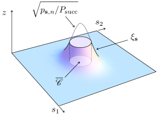
Figure 1: Plot of $\xi_{{\bf s},n}$ ($z$ axis) for large $n$ (the truncated bell-shaped surface). The figure also shows the complement of the coincidence set and $\sqrt{p_{{\bf s},n}/P_{\rm succ}}$ for $P_{\rm succ}>\min_{{\bf s}\in\widetilde{\mathscr{P}}_{n}}p_{{\bf s},n}$.

For $P_{\rm succ}>\min_{{\bf s}\in\widetilde{\mathscr{P}}_{n}}p_{{\bf s},n}$ the problem becomes more involved, as the constraint (51) is now non-trivial and ${\mathscr{C}}\not=\emptyset$. Since $p_{{\bf s},n}/P_{\rm succ}$ is bell-shaped, the complement of the coincidence set is the ‘ellipsoid’ $\overline{\mathscr{C}}_{\alpha}:=\{{\bf s}\in\widetilde{\mathscr{P}}_{n}:({\bf s}-{\bf s}_{0})^{t}\widetilde{\bf\Sigma}^{-1}({\bf s}-{\bf s}_{0})\leq\alpha^{2}$, for some $\alpha$ (Fig. 1 shows a two-dimensional version of it), and we have the solution

$$\xi_{{\bf s}}=\begin{cases}\sqrt{p_{\alpha,n}/{P_{\rm succ}}}&\text{if}\quad{\bf s}\in\overline{\mathscr{C}}_{\alpha}\\[6.99997pt] \sqrt{p_{{\bf s},n}/{P_{\rm succ}}}&\text{if}\quad{\bf s}\not\in\overline{\mathscr{C}}_{\alpha}\;,\end{cases}$$ (55)

where we have defined

$$p_{\alpha,n}:={\mathrm{e}^{-\alpha^{2}/2}\over\sqrt{(2\pi)^{r}\det\widetilde{\bf\Sigma}}},$$ (56)

and we note that the parameter $\alpha$ that gives the size of the ‘ellipsoid’ $\overline{\mathscr{C}}_{\alpha}$ is determined by normalization: $1=\sum_{\bf s}\xi_{\bf s}^{2}\simeq\int d^{r}\!{\bf s}\,\xi_{\bf s}^{2}$. Note also that the solution $\xi_{\bf s}$ is a ‘truncated’ multivariate normal distribution, as shown in Fig. 1. The above integral thus splits into two straightforward ones over the two regions in (55), and we obtain the relation:

$$P_{\rm succ}={1\over\Gamma({r\over 2})}\left(\Gamma(\mbox{\normalsize{${r\over 2}$,${\alpha^{2}\over 2}$}})+{\alpha^{r}\mathrm{e}^{-\alpha^{2}/2}\over 2^{r/2-1}r}\right),$$ (57)

where $\Gamma(a,x)$ is the upper incomplete Gamma function. Proceeding along the same line, one can compute $\sum_{\bf s}\xi_{\bf s}$ to obtain

$$F\!=\!{1\over\Gamma({r\over 2}\!+\!1)}\!\left({n\over 2m}\right)^{\!r/2}\!\!{\left[2^{r-1}r\Gamma({r\over 2},\!{\alpha^{2}\over 4})\!+\!\alpha^{r}\mathrm{e}^{-\alpha^{2}\!/4}\!\right]^{\!2}\over 2^{r/2-1}r\Gamma({r\over 2},\!{\alpha^{2}\over 2})\!+\!\alpha^{r}\mathrm{e}^{-\alpha^{2}\!/2}}.$$ (58)

Eqs. (57) and (58) give the solution to our optimization problem in parametric form, in terms of $\alpha$. Finding the fidelity $F$ as a explicit function of $P_{\rm succ}$ would require inverting the relation (57), which cannot be done analytically for an arbitrary success probability. We can however obtain an analytic expression of $F$ for a success probability close to one, i.e., for $P_{\rm succ}=1-\eta$, $\eta\ll 1$, by simply expanding the right hand side of Eq. (57) to leading order in $\alpha$. Such expansion reads:

$$\eta=1-P_{\rm succ}={\alpha^{2+r}\over 2^{1+r/2}\;\Gamma(2+r/2)}+{\cal O}(\alpha^{r+3}).$$ (59)

Solving for $\alpha$ and substituting in the expansion (at leading order in $\alpha$) of the right hand side of Eq. (58) one obtains

$$F=\left(4{n\over m}\right)^{r/2}\left[1+(1-2^{-r/2})\;\eta\right]+{\cal O}(\eta^{2}).$$ (60)

Eqs. (57) through (60) hold provided $P_{\rm succ}$ does not exponentially vanish with $n$. If it does, as in (10), where we assumed that $P_{\rm succ}<\min_{{\bf s}\in\widetilde{\mathscr{P}}_{n}}p_{{\bf s},n}$, we obtain the better scaling $F\sim(n/\sqrt{m})^{r}$. The reason for this different scaling is that a multivariate normal distribution only approximates $p_{{\bf s},n}$ accurately around its peak, whereas it falls off exponentially with $n$ at the tails (where $\min_{{\bf s}\in\widetilde{\mathscr{P}}_{n}}p_{{\bf s},n}$ lies).

Appendix B Proof of theorem 1

Proof. The proof follows the same lines of the proofs of theorems 4 and 5 in Ref. tqc2010S . Let $\mathscr{C}_{m}$ be a quantum operation transforming states on $\mathcal{H}_{\rm in}$ into sates on $\mathcal{H}^{\otimes m}$. First, we suppose that the output states of $\mathscr{C}_{m}$ have support contained in the symmetric subspace of $\mathcal{H}^{\otimes m}$. In this case, it is useful to consider the universal measure-and-prepare channel $\mathcal{M}$ defined by

$$\mathscr{M}(\rho)=\int{\rm d}\psi~{}d_{m}^{+}\,\rm{tr}[\psi^{\otimes m}\rho]~{}\psi^{\otimes m}$$

where ${\rm d}\psi$ is the invariant measure over the pure states, $d_{m}^{+}=\binom{m+d-1}{d-1}$ is the dimension of the symmetric subspace. Note that the map $\mathscr{M}$ is trace-preserving for all states with support in the symmetric subspace. Moreover, $\mathscr{M}$ provides a good approximation of the partial trace tqc2010S :

$$\left\|{\rm{tr}}_{m-k}-{\rm{tr}}_{m-k}\circ\mathscr{M}\right\|_{\diamond}\leq\frac{2kd}{m}\,,$$ (61)

where $\|\mathscr{L}\|_{\diamond}$ denotes the diamond norm of a linear, Hermitian-preserving map $\mathscr{L}$, defined as

$$\|\mathscr{L}\|_{\diamond}:=\sup_{r\in\mathbb{N}}\,\sup_{\begin{array}[]{c}|\Psi\rangle\in\mathcal{H}_{\rm in}\otimes\mathbb{C}^{r}\\ \||\Psi\rangle\|=1\end{array}}\,{\rm{tr}}\left|(\mathscr{L}\otimes\mathscr{I}_{r})(|\Psi\rangle\langle\Psi|)\right|\,,$$

$\mathscr{I}_{r}$ denoting the identity map for an $r$-dimensional quantum system. Using Eq. (61), it is immediate to construct the desired PM protocol. The protocol consists in performing the quantum operation $\mathscr{C}_{m}$ and subsequently applying the measure-and-prepare channel $\mathscr{M}$. Mathematically, it is described by the quantum operation $\widetilde{\mathscr{C}}_{m}=\mathscr{M}\circ\mathscr{C}_{m}$. Since $\mathscr{M}$ is trace-preserving (in the symmetric subspace), one has

$${\rm tr}[\widetilde{\mathscr{C}}_{m}(\rho)]={\rm tr}[{\mathscr{C}}_{m}(\rho)]$$

for every input state $\rho$, that is, $\widetilde{\mathscr{C}}_{m}$ and $\mathscr{C}_{m}$ have the same success probability. Moreover, one has the bound

$$\left\|{\rm{tr}}_{m-k}\circ\mathscr{C}_{m}-{\rm{tr}}_{m-k}\circ\widetilde{\mathscr{C}}_{m}\right\|_{\diamond}$$

$$\qquad\qquad\leq\|\left({\rm{tr}}_{m-k}-{\rm{tr}}_{m-k}\circ\mathscr{M}\right)\mathscr{C}_{m}\|_{\diamond}$$

$$\qquad\qquad\leq\|{\rm{tr}}_{m-k}-{\rm{tr}}_{m-k}\circ\mathscr{M}\|_{\diamond}\|\mathscr{C}_{m}\|_{\diamond}$$

$$\qquad\qquad\leq\frac{2kd}{m}\,,$$ (62)

having used the fact that $\|\mathscr{C}_{m}\|_{\diamond}\leq 1$ by definition. In words, the $k$-copy restrictions of $\widetilde{\mathscr{C}}_{m}$ and $\mathscr{C}_{m}$ are close to each other provided that $k\ll m$.

Now, suppose that the output of $\mathscr{C}_{m}$ has support outside the symmetric subspace. In this case, the invariance under permutations implies that $\mathscr{C}_{m}$ has a Stinespring dilation of the form

$$\mathscr{C}_{m}={\rm{tr}}_{\mathcal{H}_{E}}\circ\mathscr{K}_{m}\qquad\mathscr{K}(\rho):=K_{m}\rho K_{m}^{\dagger},$$

where $\mathcal{H}_{E}=\mathcal{H}^{\otimes m}$ and $K_{m}$ is an operator with range contained in the symmetric subspace of $\mathcal{H}^{\otimes m}\otimes\mathcal{H}_{E}\simeq(\mathcal{H}\otimes\mathcal{H})^{\otimes m}$ (for a proof see e.g. tqc2010S ). Hence, we can take the measure-and-prepare quantum operation $\widetilde{\mathscr{K}}_{m}:=\mathscr{M}_{E}\circ\mathscr{K}_{m}$, where $\mathscr{M}_{E}$ is the universal measure-and-prepare channel on $\mathcal{H}^{\otimes m}\otimes\mathcal{H}_{E}$, and we can define $\widetilde{\mathscr{C}}_{m}:={\rm{tr}}_{\mathcal{H}_{E}}\circ\widetilde{\mathscr{K}}_{m}$. By definition, the success probability of $\widetilde{\mathscr{C}}_{m}$ is equal to the success probability of $\mathscr{C}_{m}$. Moreover, one has the relation

$$\left\|{\rm{tr}}_{m-k}\circ\mathscr{C}_{m}-{\rm{tr}}_{m-k}\circ\widetilde{\mathscr{C}}_{m}\right\|_{\diamond}$$

$$\qquad\qquad=\left\|{\rm{tr}}_{m-k}\circ{\rm{tr}}_{\mathcal{H}_{E}}\circ\left(\mathscr{K}_{m}-\widetilde{\mathscr{K}}_{m}\right)\right\|_{\diamond}$$

$$\qquad\qquad=\left\|{\rm{tr}}_{\mathcal{H}^{k}_{E}}\circ\left({\rm{tr}}_{m-k}\otimes{\rm{tr}}_{\mathcal{H}^{m-k}_{E}}\right)\circ\left(\mathscr{K}_{m}-\widetilde{\mathscr{K}}_{m}\right)\right\|_{\diamond}$$

where $\rm{tr}_{\mathcal{H}_{E}^{k}}$ denotes the partial trace over $k$ ancillary Hilbert spaces. Hence, one gets the bound

$$\left\|{\rm{tr}}_{m-k}\circ\mathscr{C}_{m}-{\rm{tr}}_{m-k}\circ\widetilde{\mathscr{C}}_{m}\right\|_{\diamond}$$

$$\qquad\qquad\leq\left\|{\rm{tr}}_{\mathcal{H}^{k}_{E}}\right\|_{\diamond}\left\|\left({\rm{tr}}_{m-k}\otimes{\rm{tr}}_{\mathcal{H}^{m-k}_{E}}\right)\left(\mathscr{K}_{m}-\widetilde{\mathscr{K}}_{m}\right)\right\|_{\diamond}$$

$$\qquad\qquad\leq\frac{2d^{2}k}{m}\,,$$ (63)

having used Eq. (62) with $\widetilde{\mathscr{C}}_{m}$, $\mathscr{C}_{m}$, and $d$ replaced by $\widetilde{\mathscr{K}}_{m}$, $\mathscr{K}_{m}$, and $d^{2}$, respectively.

Finally, the error probability in distinguishing between $\widetilde{\mathscr{C}}_{m}$ and $\mathscr{C}_{m}$ by inputting a state $\rho$ and measuring $k$ output system is equal to the error probability in distinguishing between the two states

$$\widetilde{\rho}_{m,k}=\frac{{\rm{tr}}_{M-k}[\widetilde{\mathscr{C}}_{m}(\rho)]}{\rm{tr}[\widetilde{\mathscr{C}}_{m}(\rho)]}\quad{\rm and}\quad\rho_{m,k}=\frac{{\rm{tr}}_{M-k}[{\mathscr{C}}_{m}(\rho)]}{\rm{tr}[{\mathscr{C}}_{m}(\rho)]}\,,$$

respectively. Assuming equal prior probabilities for the two quantum operations, Helstrom theorem gives the bound $p_{\rm err}=\frac{1}{2}\left[1+\frac{1}{2}\|\widetilde{\rho}_{m,k}-\rho_{m,k}\|_{1}\right]$ and therefore we have

$$p_{\rm err} \leq\frac{1}{2}\left[1+\frac{\|{\rm{tr}}_{m-k}\circ(\widetilde{\mathscr{C}}_{m}-\mathscr{C}_{m})\|_{\diamond}}{2P_{\rm succ}(\rho)}\right]$$

$$\leq\frac{1}{2}\left[1+\frac{kd^{2}}{mP_{\rm succ}(\rho)}\right]\,,$$

where $P_{\rm succ}(\rho):={\rm{tr}}[\mathscr{C}_{m}(\rho)]\equiv{\rm{tr}}[\widetilde{\mathscr{C}}_{m}]\,.$ $\blacksquare$

Appendix C Approximation of the optimal $k$-copy cloning fidelity

Suppose that we are given $n$ copies of the state $|\psi_{x}\rangle\in\mathcal{H}$, $x\in\sf X$ and that we want to produce $m$ approximate copies, whose quality is assessed by checking a random group of $k$ output systems. Let $\mathscr{C}_{n,m}$ be the quantum operation describing the cloning process. Since the $k$ systems are chosen at random, we can restrict our attention to quantum operations that are invariant under permutation of the output spaces. Conditional on the occurrence of the quantum operation $\mathscr{C}_{n,m}$ and on preparation of the input $|\psi_{x}\rangle$, the $k$-copy cloning fidelity is given by

$$F_{k,x}[\mathscr{C}_{n,m}] =\frac{O_{k,x}[\mathscr{C}_{n,m}]}{P_{x}[\mathscr{C}_{n,m}]}$$ (64)

$$O_{k,x}[\mathscr{C}_{n,m}] :=\langle\varphi_{x}|^{\otimes k}{\rm{tr}}_{m-k}[\mathscr{C}_{n,m}\left(\varphi_{x}^{\otimes n}\right)]|\varphi_{x}\rangle^{\otimes k}$$

$$P_{x}[\mathscr{C}_{n,m}] :={\rm{tr}}[\mathscr{C}_{n,m}\left(\varphi_{x}^{\otimes n}\right)]\,,$$

where $\psi_{x}$ denotes the rank-one projector $\psi_{x}:=|\psi_{x}\rangle\langle\psi_{x}|$. Now, constructing the quantum operation $\widetilde{\mathscr{C}}_{n,m}$ as in theorem 1 and using Eq. (63) we have

$$\left|O_{k,x}[\mathscr{C}_{n,m}]-O[\widetilde{\mathscr{C}}_{n,m}]\right| \leq\frac{2kd^{2}}{m}$$

$$P_{x}[\mathscr{C}_{n,m}] =P_{x}[\widetilde{\mathscr{C}}_{n,m}]\equiv P_{\rm succ}\left(\psi_{x}^{\otimes n}\right),$$

and, therefore,

$$\left|F_{k,x}[\mathscr{C}_{n,m}]-F_{k,x}[\widetilde{\mathscr{C}}_{n,m}]\right|\leq\frac{2kd^{2}}{mP_{\rm succ}\left(\psi_{x}^{\otimes n}\right)}\qquad\forall x\in\sf X\,.$$

In conclusion, as long as the probability of success $P_{\rm succ}(\psi_{x}^{\otimes n})$ is lower bounded by a finite value independent of $m$, the $k$-copy fidelities of the cloning processes $\mathscr{C}_{n,m}$ and $\widetilde{\mathscr{C}}_{n,m}$. Since the bound holds for arbitrary quantum operations, in particular it holds for the quantum operation describing the optimal cloner with given probability of success.

It is immediate to extend the derivation to the Bayesian scenario where the input state $|\psi_{x}\rangle^{\otimes n}$ is given with probability $p_{x}$ and one considers the average fidelity and average success probability. Indeed, the average $k$-copy fidelity is given by

$$F_{k}[\mathscr{C}_{n,m}] =\frac{O_{k}[\mathscr{C}_{n,m}]}{P[\mathscr{C}_{n,m}]}$$

$$O_{k}[\mathscr{C}_{n,m}] :=\sum_{x}p_{x}\,O_{k,x}[\mathscr{C}_{n,m}]$$

$$P[\mathscr{C}_{n,m}] :=\sum_{x}p_{x}\,P_{x}[\mathscr{C}_{n,m}]$$

and one has the bound

$$F_{k}[\mathscr{C}_{n,m}] \leq\frac{2kd^{2}}{mP_{\rm succ}}\,,$$

$P_{\rm succ}$ being the average success probability. Again, for every fixed value of the success probability, the fidelity of the optimal cloner is achieved by a PM protocol.

Appendix D Lower bound on the average probability of success

We now show that for every fixed $n$, the probability of success of the optimal cloner is lower bounded by a finite value. Precisely, we prove the following

Lemma 1.

The quantum operation $\mathscr{C}_{n,m}^{*}$ corresponding to the $n$-to-$m$ cloner that maximizes the fidelity in Eq. (64) can be chosen without loss of generality to have success probability $P_{\rm succ}^{*}$ equal to $1/\|\tau^{-1}\|_{\infty}$, where $\tau$ is the average input state $\tau:=\sum_{x}p_{x}\varphi_{x}^{\otimes n}$ and $\|\tau^{-1}\|_{\infty}$ is the maximum eigenvalue of $\tau^{-1}$.

Proof. For a generic quantum operation $\mathscr{C}_{n,m}$, the $k$-copy fidelity can be expressed in terms of its Choi operator $C_{n,m}$ as

$$F_{k}[\mathscr{C}_{n,m}] =\frac{{\rm{tr}}[\Omega\,C_{n,m}]}{{\rm{tr}}[(I^{\otimes m}\otimes\bar{\tau})C_{n,m}]}$$

$$\Omega :=\frac{1}{{\binom{m}{k}}}\sum_{\sf S}\sum_{x}\,p_{x}\,\left(\psi_{x}^{\otimes k}\right)_{\sf S}\otimes\bar{\psi}_{x}^{\otimes n}\,,$$

where the outer summation runs over all $k$-element subsets $\sf S$ of the output Hilbert spaces, $\left(\psi_{x}^{\otimes k}\right)_{\sf S}$ denotes the operator $\psi_{x}^{\otimes k}$ acting on the Hilbert spaces in the set $\sf S$, and $\bar{\tau}$ ($\bar{\psi}_{x}$) is the complex conjugate of $\tau$ ($\psi_{x}$). Following the arguments of fiuraclonS ; xieS , one can easily show that the maximum fidelity over all quantum operations is given by

$$F^{*}_{k}=\left\|\left(I^{\otimes m}\otimes\bar{\tau}^{-\frac{1}{2}}\right)\Omega\left(I^{\otimes m}\otimes\bar{\tau}^{-\frac{1}{2}}\right)\right\|_{\infty}.$$

The maximum is achieved by choosing a Choi operator $C_{n,m}^{*}$ of the form

$$C_{n,m}^{*}=\gamma~{}\left(I^{\otimes m}\otimes\bar{\tau}^{-\frac{1}{2}}\right)|\Psi\rangle\langle\Psi|\left(I^{\otimes m}\otimes\bar{\tau}^{-\frac{1}{2}}\right)$$

where $\gamma\geq 0$ is a proportionality constant and $|\Psi\rangle$ is the eigenvector of $\left(I^{\otimes m}\otimes\bar{\tau}^{-\frac{1}{2}}\right)\Omega\left(I^{\otimes m}\otimes\bar{\tau}^{-\frac{1}{2}}\right)$ with maximum eigenvalue. With this choice, the success probability $P[\mathscr{C}_{n,m}^{*}]$ is given by

$$P[\mathscr{C}_{n,m}^{*}] ={\rm{tr}}[C_{n,m}^{*}\left(I^{\otimes m}\otimes\bar{\tau}\right)]$$

$$=\gamma\,.$$

We now show that $\gamma$ can be always chosen to be larger than $1/\|\tau^{-1}\|_{\infty}$. To this purpose, note that the only constraint on $\gamma$ is that the quantum operation $\mathscr{C}_{n,m}^{*}$ must be trace non-increasing. Now, for a generic state $\rho$ one has

$$\rm{tr}[\mathscr{C}_{n,m}^{*}(\rho)] =\gamma~{}{\rm{tr}}[C_{n,m}^{*}\left(I^{\otimes M}\otimes\bar{\rho}\right)]$$

$$=\gamma~{}\langle\Psi|\left(I^{\otimes M}\otimes\bar{\tau}^{-\frac{1}{2}}\bar{\rho}\bar{\tau}^{-\frac{1}{2}}\right)|\Psi\rangle$$

$$\leq\gamma~{}\|\bar{\tau}^{-\frac{1}{2}}\bar{\rho}\bar{\tau}^{-\frac{1}{2}}\|_{\infty}$$

$$\leq\gamma~{}\|\tau^{-1}\|_{\infty}\|\rho\|_{\infty}$$

$$\leq\gamma~{}\|\tau^{-1}\|_{\infty}.$$

Hence, the choice $\gamma=1/\|\tau^{-1}\|_{\infty}$ leads to a legitimate (trace non-increasing) quantum operation. $\blacksquare$

References

(1) J.P. Dowling and G.J. Milburn, Phil. Trans. R. Soc. Lond. A 361, 1655-1674 (2003).
(2) J.L. O’Brien, A. Furusawa, and J. Vuckovic, Nature Photon. 3, 687-695 (2009).
(3) V. Giovannetti, S. Lloyd, and L. Maccone, Science 306, 1330-1336 (2004).
(4) V. Giovannetti, S. Lloyd, and L. Maccone, Nature Photon. 5, 222-229 (2011).
(5) Y. Aharonov and L. Vaidman, Phys. Rev. A 41, 11 (1990).
(6) O. Hosten and P. Kwiat, Science 319, 787 (2008).
(7) P. B. Dixon, D. J. Starling, A. N. Jordan, and J. C.
Howell, Phys. Rev. Lett. 102, 173601 (2009).
(8) D.J. Starling, P. B. Dixon, A. N. Jordan, and J. C. Howell, Phys. Rev. A 80, 041803 (2009).
(9) S. Wu and Y. Li, Phys. Rev. A 83, 052106 (2011).
(10) G. Strübi and C. Bruder, Phys. Rev. Lett. 110, 083605 (2013).
(11) N. Brunner and C. Simon, Phys. Rev. Lett. 105, 010405 (2010).
(12) O. Zilberberg, A. Romito, and Y. Gefen, Phys. Rev. Lett. 106, 080405 (2011).
(13) J. Fiurášek, New. J. Phys. 8, 192 (2006).
(14) S. Massar and S. Popescu, Phys. Rev. A 84, 052106 (2011).
(15) B. Gendra, E. Ronco-Bonvehi, J. Calsamiglia, R. Munoz-Tapia, and E. Bagan, New. J. Phys. 14, 105015 (2012)
(16) B. Gendra, E. Ronco-Bonvehi, J. Calsamiglia, R. Munoz-Tapia, and E. Bagan, Phys. Rev. Lett. 110, 100501 (2013)
(17) B. Gendra, E. Ronco-Bonvehi, J. Calsamiglia, R. Munoz-Tapia, and E. Bagan, Phys. Rev. A 88, 012128 (2013)
(18) G. Chiribella, Y. Yang, and A.C.-C. Yao, Nature Commun. 4, 2915 (2013).
(19) P. Marek, Phys. Rev. A 88, 045802 (2013).
(20) J. Combes, C. Ferrie, Z. Jiang, C. M. Caves, Phys. Rev. A 89, 052117 (2014).
(21) A. Winter, IEEE Trans. Inf. Theory 45, 2481-2485 (1999).
(24) Ralph, T. C. & Lund, A. P. Nondeterministic Noiseless Linear Amplification of Quantum Systems. Quantum Communication Measurement and Computing Proceedings of 9th International Conference, Ed. A. Lvovsky, 155-160 (AIP, New York 2009).
(25) G. Chiribella and J. Xie, Phys. Rev. Lett. 110, 213602 (2013).
(26) G.Y. Xiang, T.C. Ralph, A.P. Lund, N. Walk, and G.J. Pryde, Nat. Photonics 4, 316-319 (2010).
(27) F. Ferreyrol et al, Phys. Rev. Lett. 104, 123603(2010).
(28) M. A. Usuga, Nat. Phys. 6, 767- 771(2010).
(29) A. Zavatta, J. Fiurašek, M. Bellini, Nat. Photon. 5, 52-60 (2011).
(30) S. Kocsis, G.Y. Xiang, T.C. Ralph, and G.F. Pryde, Nat. Phys. 9, 23-28 (2013).
(31) D. Bruss, A. Ekert, C. Macchiavello, Phys. Rev. Lett. 81, 2598 (1998)
(32) J. Bae and A. Acín, Phys. Rev. Lett. 97, 030402 (2006)
(33) G. Chiribella, G. M. D’Ariano, Phys. Rev. Lett. 97, 250503 (2006)
(34) G. Chiribella, Lecture Notes in Computer Science, 6519, 9 (2011).
(35) Y. Yang and G. Chiribella, LIPICS 22, 220 (2013).
(36) G. Chiribella and Y. Yang, arXiv:1404.0990.
(37) W. K. Wootters and W. H. Zurek, Nature 299, 802 (1982).
(38) M. Marcus and H. Minc, A survey of matrix theory and matrix inequalities (Dover, New York, 1964).
(39) Supplemental Material.
(40) G. E. Andrews, Number theory, Courier Dover Publications (1994).
(41) The difference may be larger at the ends of the spectrum, where the density of points is generally more rarefied.
(42) A. Katok and B. Hasselblatt, Introduction to the modern theory of dynamical systems, Cambridge (1996).
(43) This expression is also correct for small . For large , we can replace by , the volume of the minimal polytope that contains the lattice .
(44) A.S. Holevo, Probabilistic And Statistical Aspects Of Quantum Theory,
North-Holland Series In Statistics And Probability (North-Holland, Amsterdam 1982).

References

(1) G. Chiribella, Y. Yang, and A.C.-C. Yao, Nature Commun. 4, 2915 (2013).
(2) M. Marcus and H. Minc, A survey of matrix theory and matrix inequalities (Dover, New York, 1964).
(3)E. Bombieri and j. Vaaler, Invent. math. 73, 11 (1983).
(4) I. Borosh, M Flahive, D. Rubin and B. Treybig, Proc. Amer. Math. Soc. 105, 844 (1989).
(5) G. Chiribella, Lecture Notes in Computer Science, 6519, 9 (2011).
(6) J. Fiurašek, Phys. Rev. A 70, 032308 (2004).
(7) G. Chiribella and J. Xie, Phys. Rev. Lett. 110, 213602 (2013).