Quantifying the sensitivity of oscillation experiments to the neutrino mass ordering

Abstract

Determining the type of the neutrino mass ordering (normal versus inverted) is one of the most important open questions in neutrino physics. In this paper we clarify the statistical interpretation of sensitivity calculations for this measurement. We employ standard frequentist methods of hypothesis testing in order to precisely define terms like the median sensitivity of an experiment. We consider a test statistic $T$ which in a certain limit will be normal distributed. We show that the median sensitivity in this limit is very close to standard sensitivities based on $\Delta\chi^{2}$ values from a data set without statistical fluctuations, such as widely used in the literature. Furthermore, we perform an explicit Monte Carlo simulation of the INO, JUNO, LBNE, NO$\nu$A, and PINGU experiments in order to verify the validity of the Gaussian limit, and provide a comparison of the expected sensitivities for those experiments.

I Introduction

The ordering of neutrinos masses constitutes one of the major open issues in particle physics. The mass ordering is called “normal” (“inverted”) if $\Delta m^{2}_{31}\equiv m^{2}_{3}-m^{2}_{1}$ is positive (negative). Here and in the following we use the standard parameterization for the neutrino mass states and PMNS lepton mixing matrix PDG . Finding out which of these two possibilities is realized in Nature has profound implications for the flavor puzzle, as well as phenomenological consequences for cosmology, searches for neutrino mass, and for neutrinoless double-beta decay. Therefore, the determination of the mass ordering is one of the experimental priorities in the field. In particular, with the discovery of a large value of $\theta_{13}$ An:2012eh ; Ahn:2012nd ; Abe:2012tg ; Abe:2013xua an answer within a decade or so is certainly possible and first hints may be obtained even sooner in global fits to the world’s neutrino data.

New information is expected to come from long-baseline experiments, like T2K Abe:2011ks and NO$\nu$A Ayres:2004js ; Patterson:2012zs , which look for the appearance of $\nu_{e}(\bar{\nu}_{e})$ in a beam of $\nu_{\mu}(\bar{\nu}_{\mu})$. Proposals for a more long-term time frame include LBNE Akiri:2011dv ; CDR ; Adams:2013qkq , LBNO Stahl:2012exa , a superbeam based on the ESS Baussan:2013zcy , and eventually a neutrino factory Choubey:2011zzq . Matter effects Wolfenstein:1977ue ; Barger:1980tf ; Mikheev:1986gs will induce characteristic differences between the neutrino and antineutrino channels, which in turn will allow inference of the mass ordering, see e.g., Refs. Freund:1999gy ; Barger:2000cp for early references. The fact that a comparison of neutrino and antineutrino channels is performed also implies that the leptonic CP phase $\delta$ cannot be ignored and has to be included in the analysis as well. A selective set of recent sensitivity studies for present and future proposed long baseline oscillation experiments can be found in Refs. Qian:2013nhp ; Bass:2013hla ; Barger:2013rha ; Agarwalla:2013hma ; Messier:2013sfa ; Agarwalla:2012bv ; Blennow:2013swa ; Agarwalla:2011hh ; Coloma:2012ut ; Coloma:2012ma ; Dusini:2012vc ; Ghosh:2013pfa .

Another possibility to determine the mass ordering arises from observing the energy and zenith angle dependence of atmospheric neutrinos in the GeV range, which will also have the mass ordering information imprinted by matter effects Petcov:1998su ; Akhmedov:1998ui ; Akhmedov:1998xq ; Chizhov:1998ug ; Chizhov:1999az ; Banuls:2001zn . The flux of atmospheric neutrinos follows a steep power law with energy and thus the flux in the GeV range is quite small and requires very large detectors. IceCube technology can be adapted to neutrino energies in the GeV range by reducing the spacing of optical modules, eventually leading to the PINGU extension Aartsen:2013aaa and a similar low-energy modification can also be implemented for neutrino telescopes in the open ocean, called ORCA orca . Another way to overcome the small neutrino flux is to separate neutrino and antineutrino events using a magnetic field like in the ICal@INO experiment INO ; Ghosh:2013mga (INO for short in the following). Mass ordering sensitivity calculations have been performed for instance in Refs. Mena:2008rh ; FernandezMartinez:2010am ; Akhmedov:2012ah ; Agarwalla:2012uj ; Franco:2013in ; Ribordy:2013xea ; Winter:2013ema ; Blennow:2013vta ; Ge:2013zua for PINGU/ORCA and in Refs. TabarellideFatis:2002ni ; PalomaresRuiz:2004tk ; Indumathi:2004kd ; Petcov:2005rv ; Samanta:2006sj ; Gandhi:2007td ; Kopp:2007ai ; Blennow:2012gj ; Ghosh:2012px for INO or similar setups.

Finally, the interference effects between the oscillations driven by $\Delta m_{21}^{2}$ and $\Delta m_{31}^{2}$ in the disappearance of $\bar{\nu}_{e}$ provide a third potential avenue for this measurement. In particular, this approach has been put forward in the context of reactor neutrinos Petcov:2001sy . JUNO JUNO ; Li:2013zyd will comprise a 20 kt detector at a baseline of about 52 km of several nuclear reactors. A similar project is also discussed within the RENO collaboration reno50 . The possibility to use a precision measurement of the $\bar{\nu}_{e}$ survival probability at a nuclear reactor to identify the neutrino mass ordering has been considered by a number of authors, e.g., Refs. Schonert:2002ep ; Choubey:2003qx ; Learned:2006wy ; Zhan:2008id ; Zhan:2009rs ; Ghoshal:2010wt ; Qian:2012xh ; Ge:2012wj ; Ciuffoli:2013ep ; Li:2013zyd ; Blennow:2013vta ; Kettell:2013eos ; Capozzi:2013psa .

This impressive experimental (and phenomenological) effort has also resulted in a renewed interest in potential issues arising from the statistical interpretation of the resulting data Qian:2012zn ; Ciuffoli:2013rza (see also Ge:2012wj ), which can be summarized as: Given that the determination of the mass ordering is essentially a binary yes-or-no type question, are the usual techniques relying on a Taylor expansion around a single maximum of the likelihood applicable in this case? The goal of this paper is to answer this question within a frequentist framework for a wide range of experimental situations, including disappearance as well as appearance measurements. The answer we find in this paper can be stated succinctly as: The currently accepted methods yield approximately the expected frequentist coverage for the median experimental outcome; quantitative corrections typically lead to a (slightly) increased sensitivity compared to the standard approach prediction. The methods applied in the following are analogous to the ones from Ref. Schwetz:2006md , where similar questions have been addressed for the discovery of $\theta_{13}$ and CP violation. In the present work we strictly adhere to frequentist methods; Bayesian statistics is used to address the neutrino mass ordering question in Ref. Blennow:2013kga , see also Refs. Qian:2012zn ; Ciuffoli:2013rza for Bayesian considerations.

The outline of our paper is as follows. We first review the principles of hypothesis testing in a frequentist framework in Sec. II, apply them to the case of the mass ordering, define the sensitivity of the median experiment and discuss the relation to the standard sensitivity based on $\Delta\chi^{2}$ values from the Asimov data set. In Sec. III we consider the Gaussian limit, where all relevant quantities, such as sensitivities can be expressed analytically. Details of the derivation can be found in App. A, as well as a discussion of conditions under which the Gaussian approximation is expected to hold. In Sec. IV we present results from Monte Carlo simulations of the INO, PINGU, JUNO, NO$\nu$A, and LBNE experiments. The technical details regarding the simulations are summarized in App. B. We show that for most cases the Gaussian approximation is justified to good accuracy, with the largest deviations observed for NO$\nu$A. In Sec. V we present a comparison between the sensitivities expected for the different proposals, illustrating how the sensitivities may evolve with date. We summarize in Sec. VI, where we also provide a table which allows to translate the traditional performance indicator for the mass ordering ($\Delta\chi^{2}$ without statistical fluctuations) into well defined frequentist sensitivity measures under the Gaussian approximation. We also comment briefly on how our results compare to those in Refs. Qian:2012zn ; Ciuffoli:2013rza .

II Terminology and statistical methods

II.1 Frequentist hypothesis testing

Let us start by reviewing the principles of frequentist hypothesis testing, see e.g., Ref. PDG . First we consider the case of so-called “simple hypotheses”, where the hypothesis we want to test, $H$, as well as the alternative hypothesis $H^{\prime}$ do not depend on any free parameters. $H$ is conventionally called null hypothesis. In order to test whether data can reject the null hypothesis $H$ we have to choose a test statistic $T$. A test statistic is a stochastic variable depending on the data which is chosen in such a way that the more extreme the outcome is considered to be, the larger (or smaller) the value of the test statistic is. Once the distribution of $T$ is known under the assumption of $H$ being true, we decide to reject $H$ at confidence level (CL) $1-\alpha$ if the observation is within the $\alpha$ most extreme results, i.e., if $T>T_{c}^{\alpha}$, where the critical value $T_{c}^{\alpha}$ is defined by

$$\int_{T_{c}^{\alpha}}^{\infty}p(T|H)dT=\alpha\,,$$ (II.1)

with $p(T|H)$ being the probability distribution function of $T$ given that $H$ is true. The probability $\alpha$ is the probability of making an “error of the first kind” (or type-I error rate), i.e., rejecting $H$ although it is true. It is custom to convert this probability into a number of Gaussian standard deviations. In this work we will adopt the convention to use a double-sided Gaussian test for this conversion, such that a hypothesis is rejected if the data is more than $n\sigma$ away (on either side) from the mean. This leads to the following conversion between $n\sigma$ and the value of $\alpha$:

$$\alpha(n)=\frac{2}{\sqrt{2\pi}}\int_{n}^{\infty}dx\,e^{-x^{2}/2}=\operatorname{erfc}\left(\frac{n}{\sqrt{2}}\right)\quad\Leftrightarrow\quad n=\sqrt{2}\operatorname{erfc}^{-1}(\alpha).$$ (II.2)

This definition implies that we identify, for instance, $1\sigma,2\sigma,3\sigma$ with a CL $(1-\alpha)$ of 68.27%, 95.45%, 99.73%, respectively, which is a common convention in neutrino physics. However, note that $n\sigma$ is sometimes defined differently, as a one-sided Gaussian limit, see e.g., Eq. (1) of Ref. Cowan:2010js . This leads to a different conversion between $n\sigma$ and $\alpha$, namely

$$n_{\text{1-sided}}=\sqrt{2}\operatorname{erfc}^{-1}(2\alpha)\,,$$ (II.3)

which would lead to a CL of 84.14%, 97.73%, 99.87% for $1\sigma,2\sigma,3\sigma$.

In order to quantify how powerful a given test is for rejecting $H$ at a given CL we have to compute the so-called “power” of the test or, equivalently, the probability of making an “error of the second kind” (or type-II error rate). This is the probability $\beta$ to accept $H$ if it is not true:

$$\beta=P(T<T_{c}^{\alpha}|H^{\prime})=\int_{-\infty}^{T_{c}^{\alpha}}p(T|H^{\prime})dT\,,$$ (II.4)

where now $p(T|H^{\prime})$ is the probability distribution function of $T$ assuming that the alternative hypothesis $H^{\prime}$ is true. Obviously, $\beta$ depends on the CL $(1-\alpha)$ at which we want to reject $H$. A small value of $\beta$ means that the rate for an error of the second kind is small, i.e., the power of the test (which is defined as $1-\beta$) is large.

The case we are interested in here (neutrino mass ordering) is slightly different, since both hypotheses (normal and inverted) may depend on additional parameters $\theta$, a situation which is called “composite hypothesis testing”. This is for instance the case of long baseline oscillation experiments, where the value of $\delta$ has a large impact on the sensitivities to the neutrino mass ordering. In this case the same approach is valid while keeping a few things in mind:

• We can reject the hypothesis $H$ only if we can reject all $\theta\in H$. Thus, with

  $$\int_{T_{c}^{\alpha}(\theta)}^{\infty}p(T|\theta\in H)dT=\alpha,$$ (II.5)

  we must chose

  $$T_{c}^{\alpha}=\max_{\theta\in H}T_{c}^{\alpha}(\theta)\,.$$ (II.6)

  This ensures that all $\theta\in H$ are rejected at confidence level $(1-\alpha)$ if $T>T_{c}^{\alpha}$.

• The rate of an error of the second kind will now depend on the true parameters in the alternative hypothesis:

  $$\beta(\theta)=P(T<T_{c}^{\alpha}|\theta\in H^{\prime})=\int_{-\infty}^{T_{c}^{\alpha}}p(T|\theta\in H^{\prime})dT\,,$$ (II.7)

  with $T_{c}^{\alpha}$ defined in Eq. (II.6). It is important to note that in a frequentist framework this cannot be averaged in any way to give some sort of mean rejection power, as this would require an assumption about the distribution of the parameters implemented in Nature (which is only possible in a Bayesian analysis Blennow:2013kga ). Sticking to frequentist reasoning, we can either give $\beta$ as a function of the parameters in the alternative hypothesis, or quote the highest and/or lowest possible values of $\beta$ within the alternative hypothesis.

II.2 Application to the neutrino mass ordering

In the search for the neutrino mass ordering, we are faced with two different mutually exclusive hypotheses, namely $H_{\rm NO}$ for normal ordering and $H_{\rm IO}$ for inverted ordering. Both hypotheses will depend on the values of the oscillation parameters (which we collectively denote by $\theta$) within the corresponding ordering. In particular, appearance experiments depend crucially on the CP-violating phase $\delta$. Hence, we have to deal with the situation of composite hypothesis testing as described above. Let us now select a specific test statistic for addressing this problem.

A common test statistic is the $\chi^{2}$ with $n$ degrees of freedom, which describes the deviation from the expected values of the outcome of a series of measurements $x_{i}$ of the normal distributions $\mathcal{N}(\mu_{i},\sigma_{i})$:

$$\chi^{2}=\sum_{i=1}^{n}\frac{(x_{i}-\mu_{i})^{2}}{\sigma_{i}^{2}}\,.$$ (II.8)

The further the observations are from the expected values, i.e., the more extreme the outcome, the larger is the $\chi^{2}$. If the mean values $\mu_{i}$ depend on a set of $p$ parameters $\theta$ whose values have to be estimated from the data one usually considers the minimum of the $\chi^{2}$ with respect to the parameters:

$$\chi^{2}_{\rm min}=\min_{\theta}\chi^{2}(\theta)\,.$$ (II.9)

According to Wilk’s theorem Wilks this quantity will follow a $\chi^{2}$ distribution with $n-p$ degrees of freedom, whereas $\Delta\chi^{2}(\theta)=\chi^{2}(\theta)-\chi^{2}_{\rm min}$ will have a $\chi^{2}$ distribution with $p$ degrees of freedom. The $\chi^{2}$ distributions have known properties, and in physics we often encounter situations where data can be well described by this method and the conditions for Wilk’s theorem to hold are sufficiently fulfilled, even when individual data points are not strictly normal distributed. In general, however, it is not guaranteed and the actual distribution of those test statistics has to be verified by Monte Carlo simulations Feldman:1997qc .

Coming now to the problem of identifying the neutrino mass ordering, one needs to select a test statistic which is well suited to distinguish between the two hypotheses $H_{\rm NO}$ and $H_{\rm IO}$. Here we will focus on the following test statistic, which is based on a log-likelihood ratio and has been used in the past in the literature:

$$T=\min_{\theta\in{\rm IO}}\chi^{2}(\theta)-\min_{\theta\in{\rm NO}}\chi^{2}(\theta)\equiv\chi^{2}_{\rm IO}-\chi^{2}_{\rm NO},$$ (II.10)

where $\theta$ is the set of neutrino oscillation parameters which are confined to a given mass ordering during the minimization. Let us stress that the choice of $T$ is not unique. In principle one is free to chose any test statistic, although some will provide more powerful tests than others.

Figure 1: Left: Distribution of the test statistic $T$ for our default configuration of the JUNO reactor experiment discussed in Sec. IV.1. Histograms show the results of the MC simulation based on $10^{5}$ simulated experiments and black curves correspond to the Gaussian approximation discussed in Sec. III. Right: The value of $\alpha$ as a function of the critical value $T_{c}^{\alpha}$ required for rejecting inverted (blue) and normal (red) ordering for the JUNO reactor experiment. In the purple region both mass orderings are rejected at the CL ($1-\alpha$), in the white region both orderings are consistent with data at the CL ($1-\alpha$). The dashed lines in both panels indicate $T_{c}^{\alpha}$ for $\alpha=0.01$ for both orderings. The dotted lines indicate the crossing point $T_{c}^{\rm NO}=T_{c}^{\rm IO}$. The dot-dashed line in the right panel shows an example (for $\alpha=0.1$) in which $T_{c,\textrm{IO}}^{\alpha}<T_{c,\textrm{NO}}^{\alpha}$.

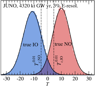
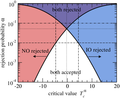
It is important to note that within a frequentist approach, rejecting one hypothesis at a given $\alpha$ does not automatically imply that the other hypothesis could not also be rejected using the same data. Instead, the only statement we can make is to either reject an ordering or not. The value of $T=0$ therefore does not a priori play a crucial role in the analysis. Let us illustrate this point at an example. In the left panel of Fig. 1, we show the distributions of the test statistics $T$ for both mass orderings obtained from the simulation of a particular configuration of the JUNO reactor experiment. Experimental details will be discussed later in Sec. IV.1. In the right panel we show the corresponding critical values $T_{c}^{\alpha}$ for testing both orderings and how they depend on the chosen confidence level $1-\alpha$. The curves for testing the different orderings cross around $\alpha=5.2\%$, indicated by the dotted lines. This represents the unique confidence level for which the experiment in question will rule out exactly one of the orderings, regardless of the experimental outcome. If, for instance, we would choose to test whether either ordering can be rejected at a confidence level of 90%, then there is a possibility of an experimental outcome $T$ with $T_{c,{\rm IO}}^{0.1}<T<T_{c,{\rm NO}}^{0.1}$, implying that both orderings could be rejected at the 90% CL. This situation is indicated by the dash-dotted line in the right panel of Fig. 1 and applies to the purple region. Thus, in order to claim a discovery of the mass ordering, it will not be sufficient to test one of the orderings. If both orderings were rejected at high confidence, it would mean either having obtained a very unlikely statistical fluctuation, underestimating the experimental errors, or neither ordering being a good description due to some new physics. Conversely, if we would choose $\alpha=0.01<0.052$ (dashed line in both panels, white region in right panel), then there is the possibility of obtaining $T_{c,{\rm NO}}^{0.01}<T<T_{c,{\rm IO}}^{0.01}$, meaning that neither ordering can be excluded at the 99% CL.

The CL corresponding to the crossing condition $T_{c,{\rm NO}}^{\alpha}=T_{c,{\rm IO}}^{\alpha}$ provides a possible sensitivity measure of a given experiment. We will refer to it as “crossing sensitivity” below. If $T_{c,{\rm NO}}^{\alpha}\approx-T_{c,{\rm IO}}^{\alpha}$ (as it is the case for the example shown in Fig. 1), this is equivalent to testing the sign of $T$. This test has been discussed also in Ref. Qian:2012zn ; Ciuffoli:2013rza . From the definition of the sensitivity of an average experiment which we are going to give in the next subsection it will be clear that the crossing sensitivity is rather different from the median sensitivity, which is typically what is intended by “sensitivity” in the existing literature. It should also be noted that the critical values for the different orderings, as well as the crossing of the critical values, in general are not symmetric with respect to $T=0$. The fact that Fig. 1 appears to be close to symmetric is a feature of the particular experiment as well of the test statistic $T$. This would not be the case for instance for the statistic $T^{\prime}$ mentioned in footnote 3. Finally, note that Fig. 1 is only concerned with the critical value of $T$ and its dependence on $\alpha$. As such, it does not tell us anything about the probability of actually rejecting, for instance, inverted ordering if the normal ordering would be the true one (power of the test). As discussed above, this probability will typically also depend on the actual parameters within the alternative ordering and can therefore not be given a particular value. However, for the crossing point of the critical values, the rejection power for the other ordering is at least $1-\alpha$.

II.3 Median sensitivity or the sensitivity of an average experiment

Let us elaborate on how to compare such a statistical analysis to previous sensitivity estimates massively employed in the literature, in particular in the context of long-baseline oscillation experiments. The most common performance indicator used for the mass ordering determination is given by

$$T_{0}^{\rm NO}(\theta_{0})=\min_{\theta\in{\rm IO}}\sum_{i}\frac{[\mu_{i}^{\rm NO}(\theta_{0})-\mu_{i}^{\rm IO}(\theta)]^{2}}{\sigma_{i}^{2}}$$ (II.11)

for testing normal ordering, with an analogous definition for inverted ordering. This quantity corresponds to the test statistic $T$ defined in Eq. (II.10) but the data $x_{i}$ are replaced by the predicted observables $\mu_{i}(\theta_{0})$ at true parameter values $\theta_{0}$. Since no statistical fluctuations are included in this definition it is implicitly assumed that it is representative for an “average” experiment. (This is sometimes referred to as the Asimov data set Cowan:2010js , and $T_{0}$ is sometimes denoted as “$\overline{\Delta\chi^{2}}$” Qian:2012zn .) $T_{0}$ is then evaluated assuming a $\chi^{2}$ distribution with 1 dof in order to quote a “CL with which a given mass ordering can be identified”. In the following, we will refer to this as the “standard method” or “standard sensitivity”. Note that $T_{0}$ by itself is not a statistic, since it does not depend on any random data. The interpretation of assigning a $\chi^{2}$ distribution to it is not well defined, and is motivated by the intuition based on nested hypothesis testing (which is not applicable for the mass ordering question). In the following we show that actually the relevant limiting distribution for $T$ (but not for $T_{0}$) is Gaussian, not $\chi^{2}$.

The formalism described in section II allows a more precise definition of an “average” experiment. One possibility is to calculate the CL $(1-\alpha)$ at which a false hypothesis can be rejected with a probability of 50%, i.e., with a rate for an error of the second kind of $\beta=0.5$. In other words, the CL $(1-\alpha)$ for $\beta=0.5$ is the CL at which an experiment will reject the wrong mass ordering with a probability of 50%. We will call the probability $\alpha(\beta=0.5)$ the “sensitivity of an average experiment” or “median sensitivity”. This is the definition we are going to use in the following for comparing our simulations of the various experiments to the corresponding sensitivities derived from the standard method.

Let us note that the median sensitivity defined in this way is not the only relevant quantity in order to design an experiment, since in practice one would like to be more certain than 50% for being able to reject a wrong hypothesis. Under the Gaussian approximation to be discussed in the next section it is easy to calculate the sensitivity $\alpha$ for any desired $\beta$, once the median sensitivity is known.

III The Gaussian case for the test statistic $T$

A crucial point in evaluating a statistical test is to know the distribution of the test statistic. In general this has to be estimated by explicit Monte Carlo simulations, an exercise which we are going to report on for a number of experiments later in this paper. However, under certain conditions the distribution of the statistic $T$ defined in Eq. (II.10) can be derived analytically and corresponds to a normal distribution Qian:2012zn :

$$T=\mathcal{N}(\pm T_{0},2\sqrt{T_{0}})\,,$$ (III.1)

where $\mathcal{N}(\mu,\sigma)$ denotes the normal distribution with mean $\mu$ and standard deviation $\sigma$ and the + ($-$) sign holds for true NO (IO). In general $T_{0}^{\rm NO}$ and $T_{0}^{\rm IO}$ may depend on model parameters $\theta$. In that case the distribution of $T$ will depend on the true parameter values and we have to consider the rules for composite hypothesis testing as outlined in section II. We provide a derivation of Eq. (III.1) in App. A, where we also discuss the conditions that need to be fulfilled for this to hold in some detail. In addition to assumptions similar to the ones necessary for Wilk’s theorem to hold, Eq. (III.1) applies if

• we are dealing with simple hypotheses, or consider composite hypotheses at fixed parameter values, or

• if close to the respective $\chi^{2}$ minima the two hypotheses depend on the parameters “in the same way” (a precise definition is given via Eq. (A.21) in the appendix), or

• if $T_{0}$ is large compared to the number of relevant parameters of the hypotheses.

III.1 Simple hypotheses

Let us now study the properties of the hypothesis test for the mass ordering based on the statistic $T$ under the assumption that it indeed follows a normal distribution as in Eq. (III.1). First we consider simple hypotheses, i.e., $T_{0}$ does not depend on any free parameters. As we shall see below, this situation applies with good accuracy to the medium-baseline reactor experiment JUNO.

For definiteness we construct a test for $H_{\rm NO}$; the one for $H_{\rm IO}$ is obtained analogously. Since large values of the test statistic favor $H_{\rm NO}$ over the alternative hypothesis $H_{\rm IO}$, we would reject $H_{\rm NO}$ for too small values of $T$. Hence, we need to find a critical value $T_{c}^{\alpha}$ such that $P(T<T_{c}^{\alpha})=\alpha$ if $H_{\rm NO}$ is correct. Since $H_{\rm NO}$ predicts $T=\mathcal{N}(T_{0}^{\rm NO},2\sqrt{T_{0}^{\rm NO}})$, we obtain

$$\alpha=\frac{1}{2}\operatorname{erfc}\left(\frac{T_{0}^{\rm NO}-T_{c}^{\alpha}}{\sqrt{8T_{0}^{\rm NO}}}\right)\quad\Leftrightarrow\quad T_{c}^{\alpha}=T_{0}^{\rm NO}-\sqrt{8T_{0}^{\rm NO}}\operatorname{erfc}^{-1}\left(2\alpha\right).$$ (III.2)

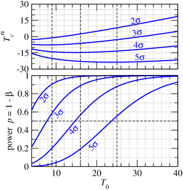
The critical values $T_{c}^{\alpha}$ as a function of $T_{0}$ are shown for several values of $\alpha$ in the upper left panel of Fig. 2. The labels in the left panel of the figure in units of $\sigma$ are based on our default convention based on the 2-sided Gaussian, Eq. (II.2).

Figure 2: Gaussian approximation for the test statistics $T$. Left upper panel: critical values for rejecting normal ordering as a function of $T_{0}$, see Eq. (III.2), for different values of $\alpha$ as labeled in the plot. Left lower panel: power of the test as a function of $T_{0}$ for different values of $\alpha$, see Eq. (III.3). Right panel: power of the test (left vertical axis) and the rate for an error of the second kind (right vertical axis) versus the CL ($1-\alpha$) for rejecting a given mass ordering for different values of $T_{0}$ as labeled in the plot. The vertical lines indicate the number of standard deviations, where we have used our standard convention Eq. (II.2) based on a 2-sided Gaussian for the solid lines and Eq. (II.3) based on a 1-sided Gaussian limit for the dashed lines. The dash-dotted red curve indicates $\alpha=\beta$, which follows in the Gaussian case from the condition $T_{c}^{\rm NO}=T_{c}^{\rm IO}$.

Let us now compute the power $p$ of the test, i.e., the probability $p$ with which we can reject $H_{\rm NO}$ at the CL $(1-\alpha)$ if the alternative hypothesis $H_{\rm IO}$ is true. As mentioned above, $p$ is related to the rate for an error of the second kind, $\beta$, since $p=1-\beta$. This probability is given by $\beta=P(T>T_{c}^{\alpha})$ for true IO, where $T_{c}^{\alpha}$ is given in Eq. (III.2). If $H_{\rm IO}$ is true we have $T=\mathcal{N}(-T_{0}^{\rm IO},2\sqrt{T_{0}^{\rm IO}})$ and hence

$$\beta=\frac{1}{2}\operatorname{erfc}\left(\frac{T_{0}^{\rm IO}+T_{c}^{\alpha}}{\sqrt{8T_{0}^{\rm IO}}}\right)\approx\frac{1}{2}\operatorname{erfc}\left(\sqrt{\frac{T_{0}}{2}}-\operatorname{erfc}^{-1}(2\alpha)\right)\,,$$ (III.3)

where the last approximation assumes $T_{0}\equiv T_{0}^{\rm NO}\approx T_{0}^{\rm IO}$, a situation we are going to encounter for instance in the case of JUNO below. We shown $p=1-\beta$ as a function of $T_{0}$ for several values of $\alpha$ in the lower left panel of Fig. 2.

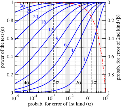
Equation (III.3) (or the lower left panel of Fig. 2) contains all the information needed to quantify the sensitivity of an experiment. In particular, it allows to address the question of how likely it is that the wrong mass ordering will be rejected at a given CL. For example, let us consider an experiment with a median sensitivity of $4\sigma$, which implies $T_{0}\approx 14.7$. If we now demand that we want to reject the wrong mass ordering with a probability of 90% ($\beta=0.1$), then this experiment will be able to do this only at slightly more than 99% CL. In the right panel of Fig. 2 we show $\beta$ as a function of $\alpha$ for several fixed values of $T_{0}$ using Eq. (III.3). This plot allows a well defined interpretation of the “$\Delta\chi^{2}$” used in the standard method (i.e., $T_{0}$) under the Gaussian approximation. For a given $T_{0}$ and a chosen sensitivity $\alpha$ we can read off the probability with which the experiment will be able to reject the wrong ordering at the ($1-\alpha$) CL.

Figure 3: Median sensitivity ($\beta=0.5$) as a function of $T_{0}$, see Eq. (III.5). The curves labeled “crossing” show the sensitivity corresponding to the condition $T_{c}^{\rm NO}=T_{c}^{\rm IO}$ according to Eq. (III.6). The solid curves use the 2-sided Gaussian to convert $\alpha$ into $n\sigma$, Eq. (II.2), whereas the dashed curves are based on the 1-sided test, Eq. (II.3). The latter correspond to the “standard sensitivity” of $n=\sqrt{T_{0}}$ and $n=\sqrt{T_{0}}/2$ for the crossing sensitivity. The edges of the green and yellow bands are obtained from the conditions on the rate for an error of the second kind $\beta=1/2\pm 0.6827/2$ and $\beta=1/2\pm 0.9545/2$, respectively.

Now it is also straight forward to compute the median sensitivity, which we have defined in section II.3 as the $\alpha$ for which $\beta=0.5$. From Eq. (III.3) we obtain

$$\alpha=\frac{1}{2}\operatorname{erfc}\left(\frac{T_{0}^{\rm IO}+T_{0}^{\rm NO}}{\sqrt{8T_{0}^{\rm IO}}}\right)\approx\frac{1}{2}\operatorname{erfc}\left(\sqrt{\frac{T_{0}}{2}}\right)\qquad\text{(median sensitivity)}.$$ (III.4)

Using our standard convention Eq. (II.2) to convert $\alpha$ into standard deviations the median sensitivity is $n\sigma$, with

$$n=\sqrt{2}\operatorname{erfc}^{-1}\left[\frac{1}{2}\operatorname{erfc}\left(\sqrt{\frac{T_{0}}{2}}\right)\right]\qquad\text{(median sensitivity)}.$$ (III.5)

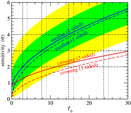
We show $n(T_{0})$ in Fig. 3. This curve corresponds to a section of the lower left panel (or right panel) of Fig. 2 at $p=0.5$. The green and yellow shaded bands indicate the CL at which we expect being able to reject NO if IO is true with a probability of 68.27% and 95.45%, respectively. The edges of the bands are obtained from the conditions $\beta=1/2\pm 0.6827/2$ and $\beta=1/2\pm 0.9545/2$, respectively. They indicate the range of obtained rejection confidence levels which emerge from values of $T$ within $1\sigma$ and $2\sigma$ from its mean assuming true IO.

Note that if we had used the 1-sided Gaussian rule from Eq. (II.3) to convert the probability Eq. (III.4) we would have obtained $n=\sqrt{T_{0}}$ for the median sensitivity. Indeed, this corresponds exactly to the “standard sensitivity” as defined in section II.3. We show this case for illustration as dashed curve in Fig. 3. The dashed vertical lines in the right panel of Fig. 2 show explicitly that using this convention we obtain $\beta=0.5$ at $n\sigma$ exactly for $T_{0}=n^{2}$. Note that with our default convention we actually obtain an increase in the sensitivity compared to $\sqrt{T_{0}}$ used in the “standard method”. The exponential nature of $\operatorname{erfc}$ implies that the difference will not be large, in particular for large $T_{0}$, see Fig. 3. For instance, the values of $T_{0}$ corresponding to a median sensitivity of $2\sigma$, $3\sigma$, $4\sigma$ according to Eq. (III.5) are 2.86, 7.74, 14.7, respectively, which should be compared to the standard case of $T_{0}=n^{2}$, i.e., 4, 9, 16. In summary, we obtain the first important result of this paper: the sensitivity obtained by using the standard method is very close to the median sensitivity within the Gaussian approximation.

Before concluding this section let us also mention the sensitivity defined by the crossing point $T_{c}^{\rm NO}=T_{c}^{\rm IO}$ discussed at the end of section II.2. This is the sensitivity $\alpha$ for which the critical values are the same for both orderings, which implies that regardless of the outcome of the experiment exactly one of the two hypotheses can be rejected at that CL. In the Gaussian approximation this implies that $\alpha=\beta$, i.e., the rates for errors of the first and second kinds are the same. Using Eq. (III.2) and the analog expression for IO we obtain by imposing $T_{c}^{\rm NO}=T_{c}^{\rm IO}$ the probability

$$\alpha=\frac{1}{2}\operatorname{erfc}\left(\frac{T_{0}^{\rm NO}+T_{0}^{\rm IO}}{\sqrt{8T_{0}^{\rm NO}}+\sqrt{8T_{0}^{\rm IO}}}\right)\approx\frac{1}{2}\operatorname{erfc}\left(\frac{1}{2}\sqrt{\frac{T_{0}}{2}}\right)\qquad(T_{c}^{\rm NO}=T_{c}^{\rm IO})\,.$$ (III.6)

The corresponding sensitivity is shown as red solid curve in Fig. 3. For this curve we use our default convention to convert $\alpha$ into $\sigma$ according to Eq. (II.2). If we instead had used the 1-sided Gaussian convention from Eq. (II.3) to convert the probability Eq. (III.6) we would have obtained the simple rule $n=\sqrt{T_{0}}/2$ (dashed red curve). This can be seen also in the right panel of Fig. 2, where the red dash-dotted curve indicates the condition $\alpha=\beta$. For a given $T_{0}$ the probability $\alpha$ for $T_{c}^{\rm NO}=T_{c}^{\rm IO}$ can be read off from the section of the corresponding blue curve with the red curve. By considering the dashed vertical lines we observe the rule $n=\sqrt{T_{0}}/2$ from the 1-sided conversion of $\alpha$ into $n\sigma$. For our default conversion it turns out that the sensitivity from the condition $T_{c}^{\rm NO}=T_{c}^{\rm IO}$ is always more than half of the median sensitivity in units of $\sigma$. From the 68.27% and 95.45% bands in Fig. 3 one can see that for a “typical” experimental outcome the sensitivity will be significantly better than the one given by the crossing condition.

III.2 Composite hypotheses

Let us now generalize the discussion to the case where $T_{0}$ depends on parameters. This will be typically the situation for long-baseline experiments, where event rates depend significantly on the (unknown) value of the CP phase $\delta$. It is straight forward to apply the rules discussed in section II assuming that $T=\mathcal{N}(T_{0}^{\rm NO}(\theta),2\sqrt{T_{0}^{\rm NO}(\theta)})$ for normal ordering and $T=\mathcal{N}(-T_{0}^{\rm IO}(\theta),2\sqrt{T_{0}^{\rm IO}(\theta)})$ for inverted ordering.

First we must ensure that we can reject NO for all possible values of $\theta$ at $(1-\alpha)$ confidence. Hence, Eq. (III.2) becomes,

$$(T_{c}^{\alpha})_{\rm min}=\min_{\theta\in{\rm NO}}\left[T_{0}^{\rm NO}(\theta)-\sqrt{8T_{0}^{\rm NO}(\theta)}\operatorname{erfc}^{-1}\left(2\alpha\right)\right]\,,$$ (III.7)

i.e., we have to choose the smallest possible $T_{c}^{\alpha}$. Considering $T_{c}^{\alpha}$ from Eq. (III.2) as a function of $T_{0}$, we see that $T_{c}^{\alpha}$ has a minimum at $T_{0}=2[\operatorname{erfc}^{-1}(2\alpha)]^{2}$, and the value at the minimum is $-2[\operatorname{erfc}^{-1}(2\alpha)]^{2}$. This minimum is also visible in Fig. 2 (upper left panel). Hence, we have

$$(T_{c}^{\alpha})_{\rm min}=\left\{\begin{array}[]{l@{\quad}c@{\quad}l}-2[\operatorname{erfc}^{-1}(2\alpha)]^{2}&\text{if}&\hat{T}_{0}^{\rm NO}<2[\operatorname{erfc}^{-1}(2\alpha)]^{2}\\ \hat{T}_{0}^{\rm NO}-\sqrt{8\hat{T}_{0}^{\rm NO}}\operatorname{erfc}^{-1}\left(2\alpha\right)&\text{if}&\hat{T}_{0}^{\rm NO}>2[\operatorname{erfc}^{-1}(2\alpha)]^{2}\end{array}\right.$$ (III.8)

where $\hat{T}_{0}^{\rm NO}$ is the minimum of $T_{0}^{\rm NO}(\theta)$ with respect to the parameters $\theta$.

The expression for the rate for an error of the second kind, Eq. (III.3) will now depend on the true values of $\theta$ in the alternative hypothesis:

$$\beta(\theta)=\frac{1}{2}\operatorname{erfc}\left[\frac{T_{0}^{\rm IO}(\theta)+(T_{c}^{\alpha})_{\rm min}}{\sqrt{8T_{0}^{\rm IO}(\theta)}}\right]\,.$$ (III.9)

The median sensitivity is obtained by setting $\beta(\theta)=0.5$. This leads to the equation $T_{0}^{\rm IO}(\theta)=-(T_{c}^{\alpha})_{\rm min}$ which has to be solved for $\alpha$. Note that this is a recursive definition, since which case in Eq. (III.8) to be used can only be decided after $\alpha$ is computed. However, it turns out that in situations of interest the first case applies. In this case we have $T_{0}^{\rm IO}(\theta)=2[\operatorname{erfc}^{-1}(2\alpha)]^{2}$. Typically it also holds that $\hat{T}_{0}^{\rm IO}\approx\hat{T}_{0}^{\rm NO}$ and therefore $\hat{T}_{0}^{\rm NO}<T_{0}^{\rm IO}(\theta)$ and $\hat{T}_{0}^{\rm NO}<2[\operatorname{erfc}^{-1}(2\alpha)]^{2}$ for $\alpha$ corresponding to the median sensitivity. Hence, we obtain the result that

$$\alpha(\theta)\approx\frac{1}{2}\operatorname{erfc}\sqrt{\frac{T_{0}^{\rm IO}(\theta)}{2}}\qquad\text{(median sensitivity)}$$ (III.10)

is a useful expression for estimating the median sensitivity for composite hypotheses in the Gaussian approximation. We will confirm this later on by comparing it to the full Monte Carlo simulations of long-baseline experiments. Also note the similarity with the expression in case of simple hypotheses (see Eq. (III.4)).

Finally we can also calculate the “crossing sensitivity” by requiring $(T_{c}^{\alpha})_{\rm min}^{\rm NO}=(T_{c}^{\alpha})_{\rm min}^{\rm IO}$, for which exactly one hypothesis can be rejected. Again this is a recursive definition, however, if $\hat{T}_{0}^{\rm NO}\simeq\hat{T}_{0}^{\rm IO}$ it turns out that only the second case in Eq. (III.8) is relevant. This leads to

$$\alpha=\frac{1}{2}\operatorname{erfc}\left(\frac{1}{\sqrt{8}}\frac{\hat{T}_{0}^{\rm NO}+\hat{T}_{0}^{\rm IO}}{\sqrt{\hat{T}_{0}^{\rm NO}}+\sqrt{\hat{T}_{0}^{\rm IO}}}\right)\approx\frac{1}{2}\operatorname{erfc}\left(\frac{1}{2}\sqrt{\frac{\hat{T}_{0}}{2}}\right)\qquad(T_{c}^{\rm NO}=T_{c}^{\rm IO})\,,$$ (III.11)

where the last relation holds for $\hat{T}_{0}\equiv\hat{T}_{0}^{\rm NO}\approx\hat{T}_{0}^{\rm IO}$, which again is very similar to the case for simple hypotheses, Eq. (III.6).

IV Monte Carlo simulations of experimental setups

Let us now apply the methods presented above to realistic experimental configurations. We have performed Monte Carlo (MC) studies to determine the sensitivity to the neutrino mass ordering for three different types of experiments, each of which obtains their sensitivity through the observation of different phenomena: ($a$) JUNO JUNO : interference (in the vacuum regime) between the solar and atmospheric oscillation amplitudes at a medium baseline reactor neutrino oscillation experiment; ($b$) PINGU Aartsen:2013aaa and INO INO : matter effects in atmospheric neutrino oscillations; ($c$) NO$\nu$A Ayres:2004js and LBNE Adams:2013qkq : matter effects in a long baseline neutrino beam experiment. In each case we have followed closely the information given in the respective proposals or design reports, and we adopted bench mark setups which under same assumptions reproduce standard sensitivities in the literature reasonably well. The specific details that have been used to simulate each experiment are summarized in App. B.

IV.1 Medium-baseline reactor experiment: JUNO

For the simulations in this paper we adopt an experimental configuration for the JUNO reactor experiment based on Refs. JUNO ; DB2-WWang ; Li:2013zyd , following the analysis described in Ref. Blennow:2013vta . A 20 kt liquid scintillator detector is considered at a distance of approximately 52 km from 10 reactors with a total power of 36 GW, with an exposure of 6 years, i.e., $4320\rm\,kt\,GW\,yr$. The energy resolution is assumed to be $3\%\sqrt{1\,{\rm MeV}/E}$. For further details see App. B.1.

The unique feature of this setup is that the sensitivity to the mass ordering is rather insensitive to the true values of the oscillation parameters within their uncertainties. Being a $\bar{\nu}_{e}$ disappearance experiment, the survival probability depends neither on $\theta_{23}$ nor on the CP phase $\delta$, and all the other oscillation parameters are known (or will be known at the time of the data analysis of the experiment) with sufficient precision such that the mass ordering sensitivity is barely affected. Therefore we are effectively very close to the situation of simple hypotheses for this setup. Note that although the mass ordering sensitivity is insensitive to the true values, the $\chi^{2}$ minimization with respect to oscillation parameters, especially $|\Delta m^{2}_{31}|$, is crucial when calculating the value of the test statistic $T$.

In the left panel of Fig. 1 we show the distribution of the test statistic $T$ from a Monte Carlo simulation of $10^{5}$ data sets for our default JUNO configuration. For each true mass ordering we compare those results to the normal distributions expected under the Gaussian approximation, namely $\mathcal{N}(T_{0}^{\rm NO},2\sqrt{T_{0}^{\rm NO}})$ for normal ordering and $\mathcal{N}(-T_{0}^{\rm IO},2\sqrt{T_{0}^{\rm IO}})$ for inverted ordering, where $T_{0}^{\rm NO}$ and $T_{0}^{\rm IO}$ are the values of the test statistic without statistical fluctuation (Asimov data set). For the considered setup we find $T_{0}^{\rm NO}=10.1$ and $T_{0}^{\rm IO}=11.1$, and we observe excellent agreement of the Gaussian approximation with the Monte Carlo simulation, see also, e.g., Ref. Qian:2012xh .

energy resolution	$3\%\sqrt{1\,{\rm MeV}/E}$		$3.5\%\sqrt{1\,{\rm MeV}/E}$
	normal	inverted	normal	inverted
$T_{0}\,(\sqrt{T_{0}}\sigma)$	10.1 ($3.2\sigma$)	11.1 ($3.3\sigma$)	5.4 ($2.3\sigma$)	5.9 ($2.4\sigma$)
median sens.	$7.3\times 10^{-4}\,(3.4\sigma)$	$4.3\times 10^{-4}\,(3.5\sigma)$	$1.0\times 10^{-2}\,(2.5\sigma)$	$7.5\times 10^{-3}\,(2.7\sigma)$
crossing sens.	$5.2\%\,(1.9\sigma)$		$12\%\,(1.6\sigma)$

Table 1: Sensitivity of the JUNO reactor experiment for $4320\rm\,kt\,GW\,yr$ exposure for two different assumptions on the energy resolution. We give the value of the test statistic without statistical fluctuation, $T_{0}$, and the “standard sensitivity” $\sqrt{T_{0}}\sigma$. The median sensitivity is calculated according to Eq. (III.4). The “crossing sensitivity” corresponds to the CL where exactly one mass ordering can be rejected regardless of the outcome, which is calculated according to Eq. (III.6).

Hence we can apply the formalism developed in section III directly to evaluate the sensitivity of the experiment in terms of $T_{0}^{\rm NO}$ and $T_{0}^{\rm IO}$. For instance, Eq. (III.4) gives for the median sensitivity $\alpha=7.3\,(4.3)\times 10^{-4}$ for testing normal (inverted) ordering, which corresponds to 3.4$\sigma$ (3.5$\sigma$). As discussed in section III those numbers are rather close to the “standard sensitivity” based on $n=\sqrt{T_{0}}$, which would give 3.2$\sigma$ (3.3$\sigma$). For the given values of $T_{0}^{\rm NO}$ and $T_{0}^{\rm IO}$ we can now use Fig. 2 to obtain the probability to reject an ordering if it is false (i.e., the power of the test) for any desired confidence level $(1-\alpha)$. The confidence level at which exactly one mass ordering can be rejected (crossing point $T_{c}^{\rm NO}=T_{c}^{\rm IO}$) is obtained from Eq. (III.6) as $\alpha=5.2\%$ or 1.9$\sigma$, see also Fig. 1. Those numbers are summarized in Tab. 1. There we give also the corresponding results for the same setup but with a slightly worse energy resolution of $3.5\%\sqrt{1\,{\rm MeV}/E}$, in which case significantly reduced sensitivities are obtained, highlighting once more the importance to achieve excellent energy reconstruction abilities. We have checked that also in this case the distribution of $T$ is very close to the Gaussian approximation.

IV.2 Atmospheric neutrinos: PINGU and INO

We now move to atmospheric neutrino experiments, which try to determine the mass ordering by looking for the imprint of the matter resonance in the angular and energy distribution of neutrino induced muons. The resonance will occur for neutrinos (antineutrinos) in the case of normal (inverted) ordering. The INO experiment INO uses a magnetized iron calorimeter which is able to separate neutrino and antineutrino induced events with high efficiency, which provides sensitivity to the mass ordering with an exposure of around 500 kt yr (10 year operation of a 50 kt detector). Alternatively, the PINGU Aartsen:2013aaa experiment, being a low-energy extension of the IceCube detector, is not able to separate neutrino and antineutrino induced muons on an event-by-event basis. This leads to a dilution of the effect of changing the mass ordering, which has to be compensated by exposures exceeding 10 Mt yr, which can be achieved for a few years of running time. In both cases the ability to reconstruct neutrino energy and direction will be crucial to determining the mass ordering.

	$\sigma_{E_{\nu}}$	$\sigma_{\theta_{\nu}}$	exposure	$T_{0}^{\rm NO}$ (med. sens.)	$T_{0}^{\rm IO}$ (med. sens.)
INO	$0.1E_{\nu}$	$10^{\circ}$	10 yr $\times$ 50 kt	5.5 ($2.6\sigma$)	5.4 ($2.6\sigma$)
PINGU	$0.2E_{\nu}$	$29^{\circ}/\sqrt{E_{\nu}/\rm GeV}$	5 yr	12.5 ($3.7\sigma$)	12.0 ($3.6\sigma$)

Table 2: Main characteristics of our default setups for INO and PINGU. We give energy resolutions for neutrino energy and direction reconstruction and default exposure. For PINGU we assume an energy dependent effective detector mass. The last two columns give the value of $T_{0}$ and the median sensitivity using Eq. (III.5) for the two orderings, assuming $\theta_{23}=45^{\circ}$.

Our simulations for the INO and PINGU experiments are based on Refs. Blennow:2012gj and Blennow:2013vta , respectively. We summarize the main characteristics of our default setups in Tab. 2, further technical details and references are given in App. B.2. Let us stress that the sensitivity of this type of experiments crucially depends on experimental parameters such a systematic uncertainties, efficiencies, particle identification, and especially the ability to reconstruct neutrino energy and direction. Those parameters are still not settled, in particular for the PINGU experiment, and final sensitivities may vary by few sigmas, see for instance Refs. Aartsen:2013aaa ; Winter:2013ema . Our setups should serve as representative examples in order to study the statistical properties of the resulting sensitivities. While the final numerical answer will depend strongly on to be defined experimental parameters, we do not expect that the statistical behavior will be affected significantly.

Figure 4: Simulated distributions of the test statistic $T$ in the INO experiment. We use our default setup as defined in Tab. 2 and assume $\theta_{23}=45^{\circ}$. Solid curves show the Gaussian approximation from Eq. (III.1).

Figure 5: Simulated distributions of the test statistic $T$ in the PINGU experiment with $\theta_{23}=40^{\circ},\,45^{\circ},\,50^{\circ}$ for the left, middle, right panel, respectively. We use our default setup as defined in Tab. 2. Solid curves show the Gaussian approximation from Eq. (III.1).

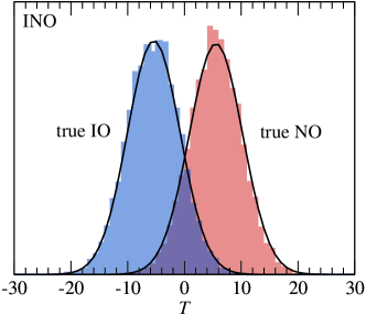
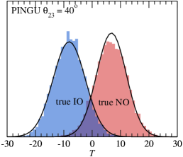
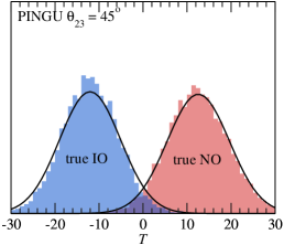
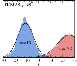
In Figs. 4 and 5 we show the distributions of the test statistic $T$ for the INO and PINGU experiments, respectively, obtained from a sample of $10^{4}$ simulated data sets for each mass ordering, using the default setups from Tab. 2. We observe good agreement with the Gaussian approximation (see also Ref. Franco:2013in for a simulation in the context of PINGU). Those results justify the use of the simple expressions from section III also for INO and PINGU in order to calculate median sensitivities or rates for errors of the first and second kind.

Figure 6: Median sensitivity for PINGU after 3 years data taking as a function of the true value of $\theta_{23}$. Left (right) panel shows a test for NO (IO), which means that the true ordering is inverted (normal). For the thick black dashed curve we consider the range $35^{\circ}<\theta_{23}<55^{\circ}$ for the true value of $\theta_{23}$ when calculating the critical value for the test statistic ($T_{c}^{\alpha}$), and the thin dashed curves indicate the corresponding 68.27% and 95.45% probability ranges of obtained rejection significances. For the blue solid curve and the corresponding green (68.27%) and yellow (95.45%) probability bands we assume that $\theta_{23}$ is known up to its octant when calculating $T_{c}^{\alpha}$. The dotted curves show the 68.27% and 95.45% probability ranges assuming that $\theta_{23}$ including its octant is known (simple hypothesis test).

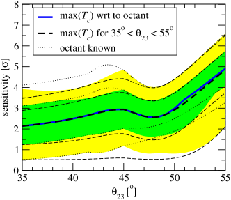
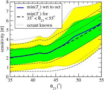
In Fig. 5 we illustrate the dependence of the distributions for PINGU on the true value of $\theta_{23}$. From this figure it is clear that the true value of $\theta_{23}$ plays an important role for the sensitivity to the mass ordering, with better sensitivity for large values of $\theta_{23}$ (a similar dependence is holds also for INO, see, e.g., Refs. Petcov:2005rv ; Blennow:2012gj ). The dependence on other parameters is rather weak (taking into account that, at the time of the experiment, $\theta_{13}$ will be known even better than today). Let us discuss the $\theta_{23}$ dependence in more detail for the case of PINGU, where from now on we use the Gaussian approximation. The problem arises when calculating the critical value for the test statistic $T$ in order to reject the null-hypothesis at a given CL. If we follow our rule for composite hypothesis, Eq. (II.6), and minimize (for NO) or maximize (for IO) $T_{c}^{\alpha}(\theta_{23})$ over $\theta_{23}$ in the range $35^{\circ}$ to $55^{\circ}$ we obtain the black dashed curves in Fig. 6. This is equivalent to using Eq. (III.10). The chosen range for $\theta_{23}$ corresponds roughly to the $3\sigma$ range obtained from current data GonzalezGarcia:2012sz . However, this may be too conservative, since at the time of the experiment T2K and NO$\nu$A will provide a very accurate determination of $\sin^{2}2\theta_{23}$. Hence, $\theta_{23}$ will be known with good precision up to its octant, see for instance Fig. 5 of Ref. Huber:2009cw . If we minimize (maximize) $T_{c}^{\alpha}(\theta_{23})$ only over the two discrete values $\theta_{23}^{\rm true}$ and $90^{\circ}-\theta_{23}^{\rm true}$ we obtain the blue solid curves in Fig. 6. The green and yellow bands indicate the corresponding 68.27% and 95.45% probability ranges of expected rejection significances. The dotted curves show the corresponding information but using only the true value of $\theta_{23}$ when calculating $T_{c}^{\alpha}$. This last case corresponds to the ideal situation of perfectly knowing $\theta_{23}$ (including its octant), in which case NO and IO become simple hypotheses. The median sensitivity for known $\theta_{23}$ is not shown in the figure for clarity, but it is very similar to the blue solid curves.

We obtain the pleasant result that all three methods give very similar values for the median sensitivity, ranging from $2\sigma$ at $\theta_{23}\simeq 35^{\circ}$ up to $5\sigma$ ($6\sigma$) rejection of NO (IO) at $\theta_{23}\simeq 55^{\circ}$. Only for the NO test and $\theta_{23}\simeq 50^{\circ}$ we find that taking the octant degeneracy into account leads to a larger spread of the 68.27% and 95.45% probability ranges for the sensitivity, implying a higher risk of obtaining a rather weak rejection. Actually, this region of parameter space (true IO and $\theta_{23}>45^{\circ}$) is the only one where the octant degeneracy severely affects the sensitivity to the mass ordering Winter:2013ema . Let us emphasize that the octant degeneracy is always fully taken into account when minimizing the $\chi^{2}$. Here we are instead concerned with the dependence of the critical value $T_{c}^{\alpha}$ on $\theta_{23}$.

IV.3 Long-baseline appearance experiments: NO$\mathbf{\nu}$A and LBNE

Long-baseline neutrino beam experiments try to identify the neutrino mass ordering by exploring the matter effect in the $\nu_{\mu}\to\nu_{e}$ appearance channel. Whether the resonance occurs for neutrinos or for antineutrinos will determine the mass ordering. A crucial feature in this case is that the appearance probability, and therefore also the event rates, depend significantly on the unknown value of the CP phase $\delta$. Most likely $\delta$ will remain unknown even at the time the mass ordering measurement will be performed, and therefore taking the $\delta$ dependence into account is essential. In the nomenclature of sections II and III we are dealing with composite hypothesis testing. In this work we consider three representative experimental configurations to study the statistical properties of the mass ordering sensitivity, namely NO$\nu$A Ayres:2004js , LBNE-10 kt, and LBNE-34 kt Adams:2013qkq , which provide increasing sensitivity to the mass ordering. Tab 3 summarizes their main features, while further details are given in App. B.3.

	L (km)	Off-axis angle	$\nu$ flux peak	Detector	M(kt)	Years $(\nu,\bar{\nu})$
NO$\nu$A	810	14 mrad	2 GeV	TASD	13 kt	(3,3)
LBNE-10(34) kt	1290	–	2.5 GeV	LAr	10(34) kt	(5,5)

Table 3: Main characteristics of the long baseline setups considered in this work. In both cases the beam power is 700 kW. The NO$\nu$A detector is a Totally Active Scintillator Detector (TASD), while for LBNE a Liquid Argon (LAr) detector is considered.

Figs. 7 and 8 show the probability distributions for the test statistic $T$ defined in Eq. (II.10), for the NO$\nu$A and LBNE-10 kt setups, respectively. The distributions are shown for both mass orderings, and for different values of $\delta$, as indicated in each panel. Our results are based on a sample of $6\times 10^{5}$ simulations for NO$\nu$A and $4\times 10^{5}$ for LBNE-10 kt per value of $\delta$, and we scan $\delta$ in steps of $10^{\circ}$. As can be seen from the figures, both the shape and mean of the distributions present large variations with the value of $\delta$. From the comparison between the two figures it is clear that the NO$\nu$A experiment will achieve very limited sensitivity to the mass ordering. On the other hand, for the LBNE-10 kt setup the situation is much better: the overlapping region is reduced, and is only sizable for certain combinations of values of $\delta$ in the two mass orderings.

Figure 7: The simulated distributions of the test statistic $T$ in the NO$\nu$A experiment for different true values of $\delta$, as indicated by the labels. The red (blue) distributions assume a true normal (inverted) ordering.

Figure 8: The simulated distributions of the test statistic $T$ in the LBNE-10 kt experiment for different true values of $\delta$, as indicated by the labels. The red (blue) distributions assume a true normal (inverted) ordering. Solid curves indicate the Gaussian approximation for $T$ from Eq. (III.1).

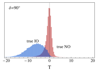
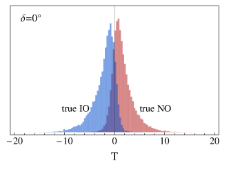
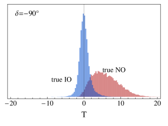
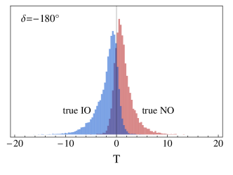
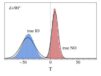
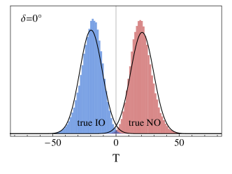
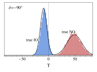
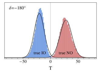
We also note that for NO$\nu$A there are clear deviations from the Gaussian shape for the $T$ distributions, while for the LBNE-10 kt experiment they are close to the Gaussian approximation discussed in section III, namely $T=\mathcal{N}(\pm T_{0}(\theta),2\sqrt{T_{0}(\theta)})$. For comparison, in Fig. 8 the Gaussian approximation is overlaid on the histograms from the Monte Carlo. Those results are in agreement with the considerations of App. A. As discussed there, one expects that the median of the $T$ distribution should remain around $\pm T_{0}$, even if corrections to the shape of the distribution are significant. We have checked that this does indeed hold for NO$\nu$A. Furthermore, assuming that there is only one relevant parameter ($\delta$ in this case), Eq. (A.24) implies that deviations from Gaussianity can be expected if $T_{0}\sim 1$, which is the case for NO$\nu$A, whereas for $T_{0}\gg 1$ (such as for LBNE) one expects close to Gaussian distributions for $T$.

One can also notice in Figs. 7 and 8 that the shape of the distributions for a given value of $\delta$ in one ordering is rather similar to the mirrored image of the distribution corresponding to the other mass ordering and $-\delta$. The reason for this is the well-known fact that the standard mass ordering sensitivity is symmetric between changing the true ordering and $\delta\to-\delta$, i.e., $T_{0}^{\rm NO}(\delta)\approx T_{0}^{\rm IO}(-\delta)$, see e.g., Figs. 8 and 9 of Ref. Patterson:2012zs and Fig. 4-13 of Ref. Adams:2013qkq . Furthermore, using the formalism in App. A, in particular Eq. (A.24), one can show that also the deviations from the Gaussian distribution will obey the same symmetry. Below we will show that despite the deviations from Gaussianity for NO$\nu$A, the final sensitivities obtained from the Monte Carlo will be surprisingly close to the Gaussian expectation. As expected, this will be even more true for LBNE-10 kt.

Figure 9: The critical value $T_{c}$ corresponding to 95% confidence level as a function of the CP-violating phase $\delta$ for NO$\nu$A (left panel) and LBNE-34 kt (right panel). The solid (dashed) lines correspond to testing the normal (inverted) ordering. The red (blue) region corresponds to values of $T$ which would reject all parameter values in the normal (inverted) ordering and thereby reject normal (inverted) ordering at 95% confidence level. In the white region, there are parameter values in both orderings which are allowed, while in the purple region none of the two orderings would be compatible with data at 95% CL.

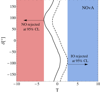
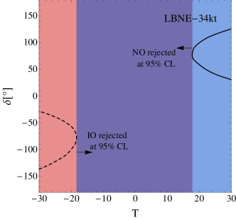
Due to the strong dependence on the CP phase $\delta$ we need to choose the critical value $T_{c}^{\alpha}$ such that the null hypothesis can be rejected at $(1-\alpha)$ CL for all possible values of $\delta$, see discussion in sections II and III.2. This is illustrated in Fig. 9, which is analogous to Fig. 1 (right panel) for a fixed CL. The continuous (dashed) black curves in Fig. 9 show the values of $T_{c}^{\alpha}$ that lead to the probability of 5% to find a smaller (larger) value of $T$ under the hypothesis of a true normal (inverted) ordering as a function of the true value of $\delta$. The left panel shows the result for NO$\nu$A, while the right panel corresponds to LBNE-34 kt. The number of data sets simulated for LBNE-34 kt in this case is $10^{5}$ per value of $\delta$, which is again scanned in steps of $10^{\circ}$. As discussed in Sec. II, a composite null hypothesis can only be rejected if we can reject all parameter sets $\theta\in H$. In our case, this would imply rejecting the hypothesis for all values of $\delta$. Therefore, in order to guarantee a CL equal to $(1-\alpha)$, the most conservative value of $T_{c}^{\alpha}$ will have to be chosen. This automatically defines two values $T^{\alpha}_{c}({\rm NO})$ and $T_{c}^{\alpha}({\rm IO})$, which are the values which guarantee that a given hypothesis can be rejected at the 95% CL. These values will generally be different, and are indicated in the figures by the arrows. In Fig. 9 we encounter the two situations already discussed in Sec. II (cf. Fig. 1):

• $T^{\alpha}_{c}({\rm IO})>T^{\alpha}_{c}({\rm NO})$: this is the case of NO$\nu$A, left panel. There is an intermediate region (shown in white) in which none of the hypotheses would be rejected at $(1-\alpha)$ CL. The reason why this intermediate region appears is because the experiment is not sensitive enough to the observable we want to measure, and a measurement at the chosen CL may not be reached.

• $T^{\alpha}_{c}({\rm IO})<T^{\alpha}_{c}({\rm NO})$: this is the case of LBNE-34 kt, right panel. There is an overlap region (shown in purple) in which both hierarchies would be rejected at $(1-\alpha)$ CL. A statistical fluctuation may bring the result of the experiment into this region, although this would typically not be expected.

The intermediate case $T^{\alpha}_{c}({\rm IO})=T^{\alpha}_{c}({\rm NO})$ would correspond to the “crossing point” discussed in Sec. II, Fig. 1, which defines the CL at which exactly one of the hypotheses can be excluded.

Figure 10: Probability of accepting normal ordering if inverted ordering is true (i.e., rate for an error of the second kind) as a function of the true $\delta$ in IO for the NO$\nu$A (left panel) and LBNE-10 kt (right panel) experiments. The different curves correspond to tests at 1$\sigma$, 2$\sigma$, 3$\sigma$ confidence level, as labeled in the plot. Furthermore the corresponding critical values $T^{\alpha}_{c}$ are given. The horizontal dotted lines indicate the median experiment, $\beta=0.5$.

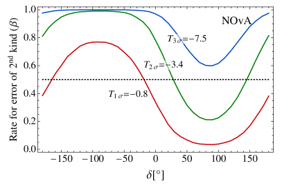
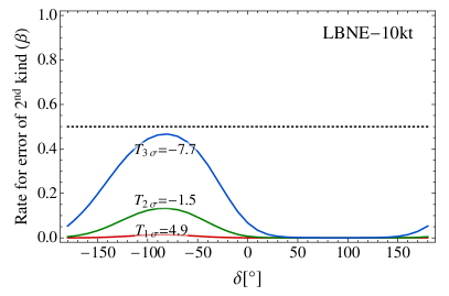
Let us now evaluate the rate for an error of the second kind corresponding to a given value of $\alpha$. After the value of $T_{c}^{\alpha}$ is determined for a given hypothesis and $\alpha$, we can compute the rate for an error of the second kind, $\beta$, as a function of the true value of $\delta$, as discussed in Sec. II. We show this probability in Fig. 10 for the NO$\nu$A and the LBNE-10 kt experiments in the left- and right-hand panels, respectively. To be explicit, we show the probability of accepting normal ordering at 1$\sigma$, 2$\sigma$, 3$\sigma$ CL, i.e., $\alpha=32\%,4.55\%,0.27\%$, (regardless of the value of $\delta$ in the NO) although the true ordering is inverted. This probability depends on the true value of $\delta$ in the IO, which is shown on the horizontal axis. By doing a cut at $\beta=0.5$ on the left-hand panel (indicated by the dotted line), we can get an idea on the median sensitivity that will be obtained for NO$\nu$A: for $\delta=-90^{\circ}$ it will be around $1\sigma$, while for $\delta=90^{\circ}$ it will reach almost the $3\sigma$ level. This seems to be roughly consistent with the expected standard sensitivities usually reported in the literature, see for instance Ref. Patterson:2012zs . Similarly, for LBNE-10 kt, we expect that the sensitivity for the median experiment will be around $3\sigma$ for $\delta=-90^{\circ}$, while for other values of $\delta$ we expect it to be much larger. This is also in agreement with the results from Ref. Adams:2013qkq , for instance.

Figure 11: Comparison of the median sensitivities based on a full MC simulation to the results based on the Gaussian approximation Eq. (III.10). The number of sigmas at which the normal mass ordering can be rejected with a probability of 50% are shown as a function of the true value of $\delta$ in the inverted ordering for NO$\nu$A (left panel) and LBNE-10 kt (right panel). The results obtained by a full MC simulation are shown by the solid thick lines. The results for the Gaussian approximation are shown by the dot-dashed curves while the dashed curves correspond to the “standard sensitivity”, i.e., $n=\sqrt{T_{0}}$. The dotted horizontal lines show the sensitivity corresponding to the “crossing point” defined in Sec. II, which guarantees that $\beta\lesssim\alpha$. The missing points in the curve for the MC results for LBNE-10 kt require a number of simulations above $4\times 10^{5}$ (per value of $\delta$) and are therefore not computed here. The green (yellow) band shows the range of $\sigma$ with which a false null hypothesis will be rejected in 68.27% and 95.45% of the experiments.

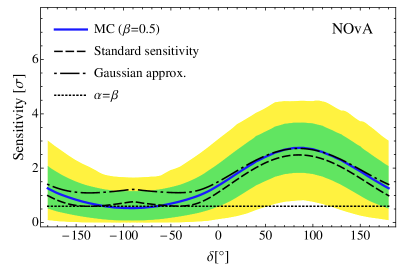
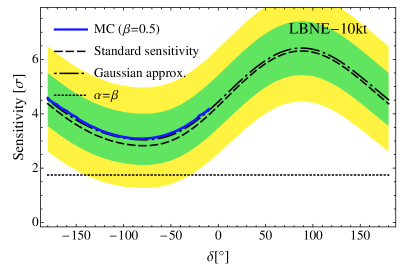
Let us now investigate in detail how our median sensitivity compares to the “standard sensitivities” widely used in the literature. In Fig. 11 the solid thick curves show the results for the median sensitivity derived from full MC simulations. The shaded green and yellow bands are analogous to those shown in Fig. 3, and show the range in the number of sigmas with which we expect to be able to reject NO if IO is true in 68.27% and 95.45% of the experiments, respectively. We also show how these results compare to the Gaussian approximation discussed in section III. The value of the $\chi^{2}$ is computed without taking statistical fluctuations into account (what is called $T_{0}$ in Sec. II). We then use Eq. (III.10) to compute the confidence level $(1-\alpha)$ at which the normal ordering can be rejected with a probability of 50% if the inverted ordering is true, as a function of the true value of $\delta$ in the IO. Then, for the dot-dashed curves we use a 2-sided Gaussian to convert $\alpha$ into number of $\sigma$, i.e., Eq. (II.2), the same prescription is also used for the MC result. We observe good agreement, in particular for LBNE. This indicates that, for the high-statistics data from LBNE, we are very close to the Gaussian limit, whereas from the smaller data sample (and smaller values of $T_{0}$) in NO$\nu$A deviations are visible, but not dramatic. We also show the results using a 1-sided Gaussian, Eq. (II.3), to convert $\alpha$ into number of sigmas, which leads to $n=\sqrt{T_{0}}$, i.e., the standard sensitivity. This is shown by the dashed lines. As discussed in Sec. II we observe that the standard sensitivity slightly under-estimates the true sensitivity. Finally, the dotted horizontal line in Fig. 11 corresponds to the significance of the crossing point $T_{c}^{\rm NO}=T_{c}^{\rm IO}$ defined in Sec. II, i.e., the confidence level at which exactly one hypothesis can be excluded regardless of the outcome of the experiment. The results are independent of the value of $\delta$, and guarantee that the rate for an error of the second kind $\beta$ is at most equal to $\alpha$, unlike for the median experiment where $\beta=0.5$. The results for the crossing point are also consistent with the Gaussian expectation Eq. (III.11).

V Comparison between facilities: future prospects

In this section we give a quantitative comparison between the different experiments that have been considered in this paper. We do a careful simulation of all the facilities using the details available in the literature from the different collaborations, see App. B for details. We have checked that our standard sensitivities are in good agreement with the respective proposals or design reports. Nevertheless, we do not explore in which way the assumptions made in the literature towards efficiencies, energy resolution, angular resolution, systematics, etc may affect the results, with the only exception of JUNO, as we explain below. Since we are mainly interested in the statistical method for determining the mass ordering, such analysis is beyond the scope of this paper. Our results will be shown as a function of the date, taking the starting points from the official statements of each collaboration. Obviously, such projections always are subject to large uncertainties.

Figure 12: The left (right) panel shows the median sensitivity in number of sigmas for rejecting the IO (NO) if the NO (IO) is true for different facilities as a function of the date. The width of the bands correspond to different true values of the CP phase $\delta$ for NO$\nu$A and LBNE, different true values of $\theta_{23}$ between $40^{\circ}$ and $50^{\circ}$ for INO and PINGU, and energy resolution between $3\%\sqrt{1~{}\textrm{MeV}/E}$ and $3.5\%\sqrt{1~{}\textrm{MeV}/E}$ for JUNO. For the long baseline experiments, the bands with solid (dashed) contours correspond to a true value for $\theta_{23}$ of $40^{\circ}$ ($50^{\circ}$). In all cases, octant degeneracies are fully searched for.

Figure 13: Probability that the wrong ordering can be rejected at $3\sigma$ (99.73% CL) for a true NO (left) and IO (right) for different facilities as a function of the date. The width of the bands has the same origin as in Fig. 12. The dotted horizontal line indicates the median experiment ($\beta=0.5$).

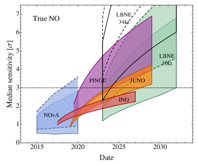
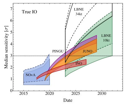
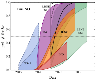
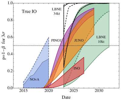
Fig. 12 shows the median sensitivities for the various experiments, i.e., the number of sigmas with which an “average experiment” for each facility can rejected a given mass ordering if it is false. In some sense this is similar to the standard sensitivity of $\sqrt{T_{0}}$ commonly applied in the literature. A different question is answered in Fig. 13, namely: what is the probability that the wrong mass ordering can be rejected at a confidence level of $3\sigma$? The confidence level has been chosen arbitrarily to $3\sigma$, based on the convention that this would correspond to “evidence” that the wrong ordering is false. Below we discuss those plots in some detail.

In order to keep the number of MC simulations down to a feasible level, we use the Gaussian approximation whenever it is reasonably justified. As we have shown in Sec. IV, this is indeed the case for PINGU, INO, and JUNO. With respect to the LBL experiments, even though we have seen that the agreement with the Gaussian case is actually quite good (see Fig. 11), there are still some deviations, in particular in the case of NO$\nu$A. Consequently, in this case we have decided to use the results from the full MC simulation whenever possible. The results for the NO$\nu$A experiment are always obtained using MC simulations, while in the case of LBNE-10 kt the results from a full MC are used whenever the number of simulations does not have to exceed $4\times 10^{5}$ (per value of $\delta$). As was mentioned in the caption of Fig. 11, this means that, in order to reach sensitivities above $\sim 4\sigma$ (for the median experiment), results from the full MC cannot be used. In these cases, we will compute our results using the Gaussian approximation instead. As mentioned in App. A, the approximation is expected to be quite accurate precisely for large values of $T_{0}$. Finally, for LBNE-34 kt, all the results have to be computed using the Gaussian approximation, since the median sensitivity for this experiment reaches the $4\sigma$ bound already for one year of exposure only, even for the most unfavorable values of $\delta$.

For each experiment, we have determined the parameter that has the largest impact on the results, and we draw a band according to it to show the range of sensitivities that should be expected in each case. Therefore, we want to stress that the meaning of each band may be different, depending on the particular experiment that is considered. In the case of long baseline experiments (NO$\nu$A, LBNE-10 kt and LBNE-34 kt), the results mainly depend on the value of the CP-violating phase $\delta$. In this case, we do a composite hypothesis test as described in Secs. II and III.2, and we draw the edges of the band using the values of true $\delta$ in the true ordering that give the worst and the best results for each setup. Nevertheless, since for these experiments the impact due to the true value of $\theta_{23}$ is also relevant, we show two results, corresponding to values of $\theta_{23}$ in the first and second octant. In all cases, the octant degeneracy is fully searched for (see App. B.3 for details). In the case of PINGU and INO, the most relevant parameter is $\theta_{23}$. We find that, depending on the combination of true ordering and $\theta_{23}$ the results will be very different. Therefore, in this case we also do a composite hypothesis test, using $\theta_{23}$ as an extra parameter. Finally, the case of JUNO is somewhat different. In this case, the uncertainties on the oscillation parameters do not have a big impact on the results. Instead, the energy resolution is the parameter which is expected to have the greatest impact, see for instance Ref. Kettell:2013eos for a detailed discussion. Therefore, in this case the width of the band shows the change on the results when the energy resolution is changed between $3\%\sqrt{1~{}\textrm{MeV}/E}$ and $3.5\%\sqrt{1~{}\textrm{MeV}/E}$. For JUNO we do a simple hypothesis test, as described in Sec. III.1.

The starting dates assumed for each experiment are: 2017 for INO INOstartingdate , 2019 for PINGU Aartsen:2013aaa and JUNO JUNO and 2022 for LBNE LBNEhomepage . Note that the official running times for PINGU and JUNO are 5 and 6 years, respectively. For illustrative purposes we extend the time in the plots to 10 years, in order to see how sensitivities would evolve under the adopted assumptions about systematics. For the NO$\nu$A experiment, we assume that the nominal luminosity will be achieved by 2014 Patterson:2012zs and we consider 6 years of data taking from that moment on.

From the comparison of Figs. 12 and 13 one can see that, even though the median sensitivity for INO would stay below the $3\sigma$ CL, there may be a sizable probability (up to $\sim 40\%$) that a statistical fluctuation will bring the result up to $3\sigma$. For NO$\nu$A, such probability could even go up to a 60%, depending on the combination of $\theta_{23}$, $\delta$ and the true mass ordering. In the case of LBNE, the dependence on the true value of $\delta$ is remarkable, in particular for the power of the test. We clearly observe the superior performance of the 34 kt configuration over the 10 kt one. For 34 kt a $3\sigma$ result can be obtained at very high probability for all values of $\delta$, and for some values of $\delta$ a much higher rejection significance of the wrong ordering is achieved with high probability.

For the atmospheric neutrino experiments INO and PINGU we show the effect of changing the true value of $\theta_{23}$ from $40^{\circ}$ to $50^{\circ}$. The effect is particularly large for PINGU and a true NO. As visible in Fig. 6, for NO the sensitivity changes significantly between $40^{\circ}$ and $50^{\circ}$, whereas for IO they happen to be similar, as reflected by the width of the bands in Figs. 12 and 13. The reason for this behavior is that for true IO and $\theta_{23}>45^{\circ}$ the mass ordering sensitivity is reduced due to the octant degeneracy Winter:2013ema . In the context of PINGU, let us stress that the precise experimental properties (in particular the ability to reconstruct neutrino energy and direction) are still very much under investigation Aartsen:2013aaa . While we consider our adopted configuration (see Sec. IV.2 and App. B.2 for details) as a representative bench mark scenario, the real sensitivity may be easily different by few standard deviations, once the actual reconstruction abilities and other experimental parameters are identified. To lesser extent this applies also to INO.

Let us also mention that in this work we only consider the sensitivity of individual experiments, and did not combine different setups. It has been pointed out in a number of studies that the sensitivity can be significantly boosted in this way Huber:2009cw ; Blennow:2012gj ; Ghosh:2012px ; Winter:2013ema ; Blennow:2013vta . We also expect that in this case, if the combined $T_{0}$ is sufficiently large, the Gaussian approximation should hold. However, we stress that a detailed investigation of this question is certainly worth pursuing in future work.

VI Discussion and summary

The sensitivity of a statistical test is quantified by reporting two numbers:

1. the confidence level $(1-\alpha)$ at which we want to reject a given hypothesis, which corresponds to a rate for an error of the first kind, $\alpha$; and

2. the probability $p$ with which a hypothesis can be rejected at CL ($1-\alpha$) if it is false (the power of the test), which is related to the rate for an error of the second kind, $\beta=1-p$ .

In this work we have applied this standard approach to the determination of the type of the neutrino mass ordering. With the help of those concepts it is straight forward to quantify the sensitivity of a given experimental configuration aiming to answer this important question in neutrino physics. We consider a test statistic $T$ (see Eq. (II.10)) in order to perform the test, which is based on the ratio of the likelihood maxima under the two hypotheses normal and inverted ordering. Under certain conditions, see App. A, the statistic $T$ is normal distributed (Gaussian approximation) Qian:2012zn . In the limit of no statistical fluctuations (Asimov data set) the test statistic $T$ becomes the usual $\Delta\chi^{2}$ (up to a sign) massively used in the literature for sensitivity calculations. In this work we denote this quantity by $T_{0}$ (in Ref. Qian:2012zn it has been denoted by $\overline{\Delta\chi^{2}}$). The sensitivity of an average experiment (in the frequentist sense) can be defined as the confidence level $(1-\alpha)$ at which a given hypothesis can be rejected with a probability $\beta=50\%$ (“median sensitivity”). An important result of our work is the following:

The sensitivity obtained by using the standard method of taking the square-root of the $\Delta\chi^{2}$ without statistical fluctuations is very close to the median sensitivity obtained within the Gaussian approximation for the test statistic $T$.

$T_{0}$	std. sens.		median sens.		lcrossing sens.m	$\beta$ for $3\sigma$	m68.27% range	a95.45% range
9	$99.73\%$	$(3.0\sigma)$	$99.87\%$	$(3.2\sigma)$	$93.32\%\,(1.8\sigma)$	$0.41$	$2.3\sigma-4.2\sigma$	$1.4\sigma-5.1\sigma$
16	$99.9937\%$	$(4.0\sigma)$	$99.9968\%$	$(4.2\sigma)$	$97.72\%\,(2.3\sigma)$	$0.11$	$3.2\sigma-5.1\sigma$	$2.3\sigma-6.1\sigma$
25	$99.999943\%$	$(5.0\sigma)$	$99.999971\%$	$(5.1\sigma)$	$99.38\%\,(2.7\sigma)$	$0.013$	$4.2\sigma-6.1\sigma$	$3.2\sigma-7.1\sigma$

Table 4: Sensitivity measures for the neutrino mass ordering in the Gaussian approximation assuming $T_{0}^{\rm NO}=T_{0}^{\rm IO}$. The columns show $T_{0}$, the standard sensitivity $n=\sqrt{T_{0}}$, the median sensitivity (Eqs. (III.4), (III.5)), the crossing sensitivity where exactly one hypothesis is rejected (equivalent to testing the sign of $T$, Eq. (III.6)), the probability $\beta$ of accepting a mass ordering at the $3\sigma$ CL although it is false (rate for an error of the second kind, Eq. (III.3)), and the range of rejection confidence levels obtained with a probability of 68.27% and 95.45%. We convert CL into standard deviations using a 2-sided Gaussian.

In section III we provide simple formulas, based on the Gaussian approximation, which allow quantification of the sensitivity in terms of error rates of the first and second kind for a given $T_{0}$. For instance, Eqs. (III.3) and (III.9) contain simple expressions for the computation of $\beta$ for given values of $\alpha$ and $T_{0}$, whereas Eq. (III.10) allows the computation of the median sensitivity in terms of $T_{0}$. In Tab. 4 we give a collection of sensitivity measures based on the Gaussian approximation for the three example values $T_{0}=9,16,25$. The columns “std. sens.” and “median sens.” demonstrate explicitly the statement emphasized above, that the median sensitivity is close to the $n=\sqrt{T_{0}}$ rule. The crossing sensitivity corresponds to the CL at which exactly one of the two hypotheses can be rejected. This is similar to testing the sign of the test statistic $T$, a test which has been discussed in Ref. Ciuffoli:2013rza and also mentioned in Ref. Qian:2012zn . By construction, this test gives smaller confidence levels than the median sensitivity and is not necessarily connected to what would be expected from an experiment. We give in the table also the probability for accepting a hypothesis at the $3\sigma$ level although it is false (rate for an error of the second kind). The last two columns in the table give the range of obtained rejection significance with a probability of 68.27% and 95.45% (assuming that the experiment would be repeated many times). Those are a few examples of how to apply the equations from section III. These sensitivity measures provide different information and all serve to quantify the sensitivity of an experiment within a frequentist framework. They can be compared to similar sensitivity measures given in Ref. Qian:2012zn in a Bayesian context (see, e.g., their Tab. IV).

In the second part of the paper we report on the results from Monte Carlo simulations for several experimental setups which aim to address the neutrino mass ordering: the medium-baseline reactor experiment JUNO, the atmospheric neutrino experiments INO and PINGU, and the long-baseline beam experiments NO$\nu$A and LBNE. In each case we have checked by generating a large number of random data sets how well the Gaussian approximation is satisfied. Our results indicate that the Gaussian approximation is excellent for JUNO, INO, and PINGU. For NO$\nu$A the $T$ distributions deviate significantly from Gaussian (strongly dependent on the true value of the CP phase $\delta$), however the Gaussian expressions for the sensitivities still provide a fair approximation to the results of the Monte Carlo. For LBNE the Gaussian approximation is again fulfilled reasonably well. This is in agreement with our analytical considerations on the validity of the Gaussian approximation given in App. A, where we find that for experiments with $T_{0}$ large compared to the number of relevant parameters Gaussiantiy should hold. Hence, we expect that the Gaussian approximation should hold to very good accuracy also for experiments with a high sensitivity to the mass ordering, such as for instance a neutrino factory Choubey:2011zzq ; Ballett:2012rz ; Christensen:2013va or the LBNO experiment Stahl:2012exa , when explicit Monte Carlo simulations become exceedingly unpractical due to the very large number of data sets needed in order to explore the high confidence levels.

In section V we provide a comparison of the sensitivities of the above mentioned facilities using the statistical methods discussed in this paper. Figures 12 and 13 illustrate how the median sensitivity and the probability to reject the wrong mass ordering at $3\sigma$ CL for the various experiments, respectively, could evolve as function of time based on official statements of the collaborations. While this type of plots is subject to large error bars on the time axis (typically asymmetric) as well as concerning actual experimental parameters, our results indicate that it is likely that the wrong mass ordering will be excluded at $3\sigma$ CL within the next 10 to 15 years.

Acknowledgments. We thank Walter Winter for comments on the PINGU sensitivity and Enrique Fernandez-Martinez for useful discussions. This work was supported by the Göran Gustafsson Foundation (M.B.) and by the U.S. Department of Energy under award number DE-SC0003915 (P.C. and P.H.). T.S. acknowledges partial support from the European Union FP7 ITN INVISIBLES (Marie Curie Actions, PITN-GA-2011-289442).

Appendix A The distribution of $T$

Consider $N$ data points $x_{i}$, and the two hypotheses, $H$ and $H^{\prime}$, and we want to test whether one of them can be rejected by the data. The theoretical predictions for the observed data under the two hypotheses are denoted by $\mu_{i}$ and $\mu^{\prime}_{i}$, respectively. The prediction $\mu_{i}$ ($\mu^{\prime}_{i}$) may depend on a set of $P$ ($P^{\prime}$) parameters $\theta_{\alpha}$ ($\theta^{\prime}_{\alpha}$) which have to be estimated from the data. For the case of the mass ordering we have $P=P^{\prime}$ and $H$ and $H^{\prime}$ depend on the same set of parameters. However, here we want to be more general.

Under $H$ the data $x_{i}$ will be distributed as $\mathcal{N}(\mu_{i}(\theta_{\alpha}^{0}),\sigma_{i})$, where $\mathcal{N}(m,\sigma)$ denotes the normal distribution with mean $m$ and variance $\sigma^{2}$ and $\theta_{\alpha}^{0}$ are the unknown true values of the parameters. If $H^{\prime}$ is true $x_{i}$ will be distributed as $\mathcal{N}(\mu^{\prime}_{i}({\theta^{\prime}}_{\alpha}^{0}),\sigma^{\prime}_{i})$. Once the experiment has been performed one can build for each hypothesis a least-square function:

$$X^{2}(\theta_{\alpha};H) =\sum_{i}\left(\frac{\mu_{i}(\theta_{\alpha})-x_{i}}{\sigma_{i}}\right)^{2}$$ (A.1)

$$X^{2}(H) =\min_{\theta_{\alpha}}\sum_{i}\left(\frac{\mu_{i}(\theta_{\alpha})-x_{i}}{\sigma_{i}}\right)^{2}=\sum_{i}\left(\frac{\mu_{i}(\hat{\theta}_{\alpha})-x_{i}}{\sigma_{i}}\right)^{2}$$ (A.2)

and similar for $H^{\prime}$. Here $\hat{\theta}_{\alpha}$ are the parameters at the minimum, which will be different for each hypothesis. In practice often the variances have to be estimated from the data itself, e.g., $\sigma_{i}\approx\sigma^{\prime}_{i}\approx\sqrt{x_{i}}$. In the following we will assume $\sigma_{i}=\sigma^{\prime}_{i}$. Let us note that generalization to correlated data is straight forward. The test statistic $T$ from Eq. (II.10) is then given by $T=X^{2}(H^{\prime})-X^{2}(H)$. In the following we will derive the distribution of $T$.

The distributions of $X(H)$ and $X(H^{\prime})$. Let us assume for definiteness that $H$ is true. First we consider $X^{2}(H)$, and we derive the well-known result, that $X^{2}(H)$ is distributed as $\chi^{2}$ with $N-P$ d.o.f. Let us define the variables

$$y_{i}(\theta_{\alpha})\equiv\frac{\mu_{i}(\theta_{\alpha})-x_{i}}{\sigma_{i}}\,.$$ (A.3)

Under $H$, the $y_{i}(\theta_{\alpha}^{0})=n_{i}$ are $N$ standard normal distributed variables with $\mathcal{N}(0,1)$. Then we have $X^{2}(H)=\text{min}_{\theta}\sum_{i}[y_{i}(\theta_{\alpha})]^{2}$. The minimum condition is

$$\frac{\partial X^{2}}{\partial\theta_{\alpha}}=2\sum_{i}y_{i}(\hat{\theta}_{\alpha})\frac{\partial y_{i}}{\partial\theta_{\alpha}}=0\,.$$ (A.4)

Asymptotically the parameter values at the minimum $\hat{\theta}_{\alpha}$ will converge to the true values $\theta_{\alpha}^{0}$. Therefore we assume

$$\left.\frac{\partial y_{i}}{\partial\theta_{\alpha}}\right|_{\hat{\theta}_{\alpha}}\approx\left.\frac{\partial y_{i}}{\partial\theta_{\alpha}}\right|_{\theta_{\alpha}^{0}}\equiv B_{i\alpha}$$ (A.5)

and expand

$$y_{i}(\hat{\theta}_{\alpha})=n_{i}+\sum_{\alpha}B_{i\alpha}(\hat{\theta}_{\alpha}-\theta_{\alpha}^{0})\,.$$ (A.6)

Here and in the following sums run over $\alpha,\beta=1,\ldots,P$ and $i,j,k=1,\ldots,N$ if not explicitly noted otherwise. Then the minimum condition Eq. (A.4) becomes

$$\sum_{i}B_{i\alpha}n_{i}+\sum_{i\beta}B_{i\alpha}B_{i\beta}(\hat{\theta}_{\beta}-\theta_{\beta}^{0})=0$$ (A.7)

and we obtain

$$X^{2}(H)=\sum_{i}[y_{i}(\hat{\theta}_{\alpha})]^{2}=\sum_{i}n_{i}^{2}-\sum_{i\alpha\beta}(\hat{\theta}_{\alpha}-\theta_{\alpha}^{0})B_{i\alpha}B_{i\beta}(\hat{\theta}_{\beta}-\theta_{\beta}^{0})\,.$$ (A.8)

Now we diagonalize the symmetric $P\times P$ matrix $B^{T}B=(\sum_{i}B_{i\alpha}B_{i\beta})$ with the orthogonal matrix $R$ as $B^{T}B=R^{T}b^{2}R$ with $b=\text{diag}(b_{\alpha})$. Then Eq. (A.7) can be written as

$$\sum_{\beta}b_{\alpha}R_{\alpha\beta}(\hat{\theta}_{\beta}-\theta_{\beta}^{0})=-\sum_{i}V_{i\alpha}n_{i}\quad\text{with}\quad V_{i\alpha}\equiv b_{\alpha}^{-1}\sum_{\beta}R_{\alpha\beta}B_{i\beta}$$ (A.9)

and

$$X^{2}(H)=\sum_{ij}n_{i}\left(\delta_{ij}-\sum_{\alpha}V_{i\alpha}V_{j\alpha}\right)n_{j}\,.$$ (A.10)

The matrix $(V_{i\alpha})$ defined in Eq. (A.9) is a rectangular $N\times P$ matrix which per construction obeys the orthogonality condition $\sum_{i}V_{i\alpha}V_{i\beta}=\delta_{\alpha\beta}$. Hence, we can always complete it by $N-P$ columns to a full orthogonal $N\times N$ matrix such that $\sum_{k}V_{ik}V_{jk}=\delta_{ij}$ and $\sum_{k}V_{ki}V_{kj}=\delta_{ij}$. Then we have

$$X^{2}(H)=\sum_{ij}n_{i}\left(\sum_{r=P+1}^{N}V_{ir}V_{jr}\right)n_{j}=\sum_{r=P+1}^{N}w_{r}^{2}\,,$$ (A.11)

where $w_{r}\equiv\sum_{i}V_{ri}n_{i}$ are $N-P$ independent variables distributed as $\mathcal{N}(0,1)$. This shows explicitly that if $H$ is true, $X^{2}(H)$ is distributed as a $\chi^{2}$ with $N-P$ d.o.f. Wilks .

Let us now derive the distribution of $X^{2}(H^{\prime})$ under the assumption that $H$ is true. Again we define

$$y^{\prime}_{i}(\theta^{\prime}_{\alpha})\equiv\frac{\mu^{\prime}_{i}(\theta^{\prime}_{\alpha})-x_{i}}{\sigma_{i}}\,,$$ (A.12)

however, now $y^{\prime}_{i}$ will not be standard normal distributed as $\mathcal{N}(0,1)$, since per assumption $x_{i}$ have mean $\mu_{i}(\theta_{\alpha}^{0})$ (and not $\mu^{\prime}_{i}$). Nevertheless we can assume that $y^{\prime}_{i}(\theta^{\prime}_{\alpha})$ can be expanded around a fixed reference point $\theta_{\alpha}^{*}$, such that the minimum in the wrong hypothesis, $\hat{\theta}^{\prime}_{\alpha}$, converges asymptotically towards it. We write

$$\left.\frac{\partial y^{\prime}_{i}}{\partial\theta_{\alpha}}\right|_{\hat{\theta}^{\prime}_{\alpha}}\approx\left.\frac{\partial y^{\prime}_{i}}{\partial\theta_{\alpha}}\right|_{\theta_{\alpha}^{*}}\equiv B^{\prime}_{i\alpha}\,,\qquad y^{\prime}_{i}(\hat{\theta}^{\prime}_{\alpha})=y^{\prime}_{i}(\theta_{\alpha}^{*})+\sum_{\alpha}B^{\prime}_{i\alpha}(\hat{\theta}^{\prime}_{\alpha}-\theta_{\alpha}^{*})\,,$$ (A.13)

and

$$y^{\prime}_{i}(\theta_{\alpha}^{*})=\frac{\mu^{\prime}_{i}(\theta^{*}_{\alpha})-x_{i}}{\sigma_{i}}=m_{i}+n_{i}=n^{\prime}_{i}\quad\text{with}\quad m_{i}\equiv\frac{\mu^{\prime}_{i}(\theta^{*}_{\alpha})-\mu_{i}(\theta^{0}_{\alpha})}{\sigma_{i}}\,.$$ (A.14)

Here $n_{i}$ are $\mathcal{N}(0,1)$ as before, but $n^{\prime}_{i}$ are $\mathcal{N}(m_{i},1)$. Now the calculation proceeds as before and we arrive at

$$X^{2}(H^{\prime})=\sum_{r=P^{\prime}+1}^{N}(w^{\prime}_{r})^{2}\,,$$ (A.15)

where $w^{\prime}_{r}\equiv\sum_{i}V^{\prime}_{ri}n^{\prime}_{i}$ are now $N-P^{\prime}$ independent normal variables with mean $\langle w^{\prime}_{r}\rangle=\sum_{i}V^{\prime}_{ri}m_{i}$. Then $X^{2}(H^{\prime})$ has a so-called non-central $\chi^{2}$ distribution with $N-P^{\prime}$ d.o.f. and a non-centrality parameter $\Delta=\sum_{r=P^{\prime}+1}^{N}\langle w^{\prime}_{r}\rangle^{2}$.

The distribution of the test statistic $T$. Let us now consider the test statistic $T=X^{2}(H^{\prime})-X^{2}(H)$. Using Eqs. (A.11) and (A.15) we find:

$$T= \sum_{ij}(m_{i}+n_{i})\left(\sum_{r=P^{\prime}+1}^{N}V^{\prime}_{ir}V^{\prime}_{jr}\right)(m_{j}+n_{j})-\sum_{ij}n_{i}\left(\sum_{r=P+1}^{N}V_{ir}V_{jr}\right)n_{j}$$ (A.16)

$$= \sum_{ij}m_{i}\left(\sum_{r=P^{\prime}+1}^{N}V^{\prime}_{ir}V^{\prime}_{jr}\right)m_{j}+2\sum_{ij}m_{i}\left(\sum_{r=P^{\prime}+1}^{N}V^{\prime}_{ir}V^{\prime}_{jr}\right)n_{j}$$ (A.17)

$$+\sum_{ij}n_{i}\left(\sum_{\alpha=1}^{P}V_{i\alpha}V_{j\alpha}-\sum_{\alpha=1}^{P^{\prime}}V^{\prime}_{i\alpha}V^{\prime}_{j\alpha}\right)n_{j}$$ (A.18)

The first term in Eq. (A.17) is just a constant, independent of the data. Using the definition of $m_{i}$ in Eq. (A.14) and comparing with Eq. (A.11) one can see that this term is identical to $X^{2}(H^{\prime})$ but replacing the data $x_{i}$ by the prediction for $H$ at the true values:

$$\sum_{ij}m_{i}\left(\sum_{r=P^{\prime}+1}^{N}V^{\prime}_{ir}V^{\prime}_{jr}\right)m_{j}=\min_{\theta^{\prime}_{\alpha}}\sum_{i}\left(\frac{\mu_{i}^{\prime}(\theta^{\prime}_{\alpha})-\mu_{i}(\theta_{\alpha}^{0})}{\sigma_{i}}\right)^{2}\equiv T_{0}\,.$$ (A.19)

This is nothing else than the usual “$\Delta\chi^{2}$” between the two hypotheses without statistical fluctuations, compare Eq. (II.11).

The second term in Eq. (A.17) is a sum of $N$ standard normal variables, $\sum_{i}a_{i}n_{i}$. This gives a normal variable with variance $\sum_{i}a_{i}^{2}$. It is easy to show from Eq. (A.17) that the variance is $4T_{0}$ and Eq. (A.17) can be written as

$$T_{0}+2\sqrt{T_{0}}n\,,$$ (A.20)

with $n$ standard normal. Hence, we find that if the term in Eq. (A.18) can be neglected, $T$ is gaussian distributed with mean $T_{0}$ and standard deviation $2\sqrt{T_{0}}$ Qian:2012zn .

Consider now the term in Eq. (A.18). Using $\langle n_{i}n_{j}\rangle=\delta_{ij}$ and the orthonormality of $V$ and $V^{\prime}$ we obtain that the mean value of this term is $P-P^{\prime}$. Hence, if the number of parameters in the two hypotheses is equal (as it is the case for the neutrino mass ordering) the mean value of $T$ remains $T_{0}$ as in the Gaussian approximation, Eq. (A.20). For testing hypotheses with different numbers of parameters the mean value will be shifted from $T_{0}$. However, even if the mean value remains unaffected, the higher moments of the distribution can still be modified. Under which conditions can the term in Eq. (A.18) be neglected?

• Obviously this term is absent if no parameters are estimated from the data, $P=P^{\prime}=0$, i.e., for simple hypotheses. This applies in particular, if we compare the two hypotheses for fixed parameters.

• The term in Eq. (A.18) will also vanish for

  $$\sum_{\alpha=1}^{P}V_{i\alpha}V_{j\alpha}=\sum_{\alpha=1}^{P^{\prime}}V^{\prime}_{i\alpha}V^{\prime}_{j\alpha}\quad\text{or}\quad VV^{T}=V^{\prime}{V^{\prime}}^{T}\,.$$ (A.21)

  This condition has a geometrical interpretation. Consider the $N$ dimensional space of data. Varying $P$ parameters $\theta_{\alpha}$ the predictions $\mu_{i}(\theta_{\alpha})$ describe a $P$ dimensional subspace in the $N$ dimensional space. The operator $VV^{T}$ is a projection operator into the tangential hyperplane to this subspace at the $X^{2}$ minimum. This can be seen by considering the definition of $V$ in Eq. (A.9) and of $B$ in Eq. (A.5), which show that $V$ is determined by the derivatives $\partial\mu_{i}/\partial\theta_{\alpha}$ at the minimum. Similar, $V^{\prime}{V^{\prime}}^{T}$ projects into the $P^{\prime}$ dimensional tangential hyperplane at the minimum corresponding to $H^{\prime}$. Hence, the condition (A.21) means that the hyperplanes of the two hypotheses have to be parallel at the minima. Obviously this condition can be satisfied only if the dimensions of the hyperplanes are the same, i.e., $P=P^{\prime}$.

  We note also that the condition (A.21) is invariant under a change of parameterization, which amounts to $B\to BS$ with $S_{\alpha\beta}\equiv\partial\theta_{\alpha}/\partial\tilde{\theta}_{\beta}$ being a $P\times P$ orthogonal matrix describing the variable transformation $\theta_{\alpha}\to\tilde{\theta}_{\alpha}$. Such a transformation would just change the orthogonal matrix $R$, but leave the operator $VV^{T}$ invariant. Roughly speaking we can say that sufficiently close to the respective minima $\theta^{0}_{\alpha}$ and $\theta^{*}_{\alpha}$, the two hypotheses should depend on the parameters “in the same way”, where the precise meaning is given by Eq. (A.21).

• Irrespective of the above conditions, we can neglect Eq. (A.18) if its variance is much smaller than the variance of the term in Eq. (A.17), which is given by $4T_{0}$. Eq. (A.18) is the difference of two $\chi^{2}$ distributions with $P$ and $P^{\prime}$ d.o.f., respectively. The $\chi^{2}_{n}$ distribution has a mean and variance of $n$ and $2n$, respectively. Hence, we should be able to neglect this term if $T_{0}\gg P,P^{\prime}$, i.e., for high sensitivity experiments.

Example with one parameter. To simplify the situation let us consider the case where just one parameter $\theta$ is estimated from the data, for both $H$ and $H^{\prime}$. The matrix $V_{i\alpha}$ defined in Eq. (A.9) becomes now just a normalized column vector

$$V_{i}=\frac{1}{\mathcal{N}}\frac{1}{\sigma_{i}}\frac{\partial\mu_{i}}{\partial\theta}\quad\text{with}\quad\mathcal{N}=\sqrt{\sum_{j}\frac{1}{\sigma_{j}^{2}}\left(\frac{\partial\mu_{j}}{\partial\theta}\right)^{2}}$$ (A.22)

and similar for $V^{\prime}_{i}$. The term in Eq. (A.18) is now just the difference of the square of two standard normal variables: $n^{2}-{n^{\prime}}^{2}$, with $n=\sum_{i}V_{i}n_{i}$ and $n^{\prime}=\sum_{i}V^{\prime}_{i}n_{i}$. As mentioned above for the general case, we see that $\langle n^{2}-{n^{\prime}}^{2}\rangle=0$. The variance of this term is obtained as

$$\langle(n^{2}-{n^{\prime}}^{2})^{2}\rangle=\sum_{ijkl}\langle n_{i}n_{j}n_{k}n_{l}\rangle(V_{i}V_{j}-V^{\prime}_{i}V^{\prime}_{j})(V_{k}V_{l}-V^{\prime}_{k}V^{\prime}_{l})=4\left[1-\left(\sum_{i}V_{i}V^{\prime}_{i}\right)^{2}\right]$$ (A.23)

where we have used that $\langle n_{i}^{4}\rangle=3$. We can write $(V^{T}V^{\prime})^{2}=\mathrm{Tr}[VV^{T}V^{\prime}{V^{\prime}}^{T}]=\cos^{2}\varphi$, where $\varphi$ is the angle between the two hyperplanes (i.e., lines, in this case) for $H$ and $H^{\prime}$. Hence we find that the variance is zero if $|V^{T}V^{\prime}|=1$, i.e., the lines are parallel. And we have a measure to estimate when Eq. (A.20) is valid, namely when the variance of Eq. (A.18) is small compared to the variance of the second term in Eq. (A.17). In the example of one parameter this means

$$1-(V^{T}V^{\prime})^{2}=\sin^{2}\varphi\ll T_{0}\,.$$ (A.24)

Since $\sin^{2}\varphi\leq 1$ we find that for $T_{0}\gg 1$ the gaussian approximation is expected to be valid if only one parameter is estimated from data.

Appendix B Simulation details

In the following, we describe the main details that have been used to simulate the experimental setups considered in this work. Unless stated otherwise the true values for the oscillation parameters have been set to the following values GonzalezGarcia:2012sz , and the $\chi^{2}$ (or the test statistic $T$) has been minimized with respect to them by adding Gaussian penalty terms to the $\chi^{2}$ with the following $1\sigma$ errors:

$$\theta_{12}=33.36^{\circ}\pm 3\%\,,\quad\sin^{2}2\theta_{13}=0.089\pm 0.005\,,\quad\sin^{2}2\theta_{23}=0.97\pm 0.05\,,$$

$$\Delta m^{2}_{21}=7.5\times 10^{-5}\,{\rm eV}^{2}\pm 2.5\%\,,\quad\Delta m^{2}_{31}=\left\{\begin{array}[]{rc}2.47\times 10^{-3}\,{\rm eV}^{2}&\,({\rm NO})\\ -2.43\times 10^{-3}\,{\rm eV}^{2}&\,({\rm IO})\end{array}\right\}\pm 10\%\,.$$ (B.3)

Unless otherwise stated, we assume the true value of $\theta_{23}$ to be in the first octant. Nevertheless, the region around $\pi/2-\theta_{23}$ would not be disfavored by the penalty term since it is added in terms of $\sin^{2}2\theta_{23}$ instead of $\theta_{23}$. Therefore, we also look for compatible solutions around $\sim\pi/2-\theta_{23}$ (the so-called octant degeneracy Fogli:1996pv ) and keep the minimum of the $\chi^{2}$ between the two.

B.1 Medium baseline reactor experiment: JUNO

We adopt an experimental configuration for the JUNO experiment based on Refs. JUNO ; DB2-WWang ; Li:2013zyd , following the analysis described in Ref. Blennow:2013vta . We normalize the number of events such that for the default exposure of $\rm 20\,kt\,\times 36\,GW\times 6\,yr=4320\,kt\,GW\,yr$ we obtain $10^{5}$ events JUNO ; DB2-WWang . The energy resolution is assumed to be $3\%\sqrt{1\,{\rm MeV}/E}$. We perform a $\chi^{2}$ analysis using 350 bins for the energy spectrum. This number is chosen sufficiently large such that bins are smaller (or of the order of) the energy resolution. We take into account an overall normalization uncertainty of 5% and a linear energy scale uncertainty of 3%. Uncertainties in the oscillation parameters $\sin^{2}\theta_{13}$ and $\sin^{2}\theta_{12}$ are included as pull parameters in the $\chi^{2}$ using true values and uncertainties according to Eq. (B.3), while $|\Delta m^{2}_{31}|$ is left free when fitting the data. For this parameter a dense grid is computed and the minimum is manually searched for. We have updated the analysis from Ref. Blennow:2013vta by taking into account the precise baseline distribution of 12 reactor cores as given in Tab. 1 of Ref. Li:2013zyd (including also the Daya Bay reactors at 215 and 265 km). This reduces $T_{0}$ by about 5 units compared to the idealized situation of a point-like source at 52.47 km (the latter being the power averaged distance of the 10 reactors not including the Daya Bay reactors). Adopting the same assumptions as in Ref. Li:2013zyd we find for a $4320\rm\,kt\,GW\,yr$ exposure $T_{0}\approx 11.8$, which is in excellent agreement with their results, see red-dashed curve in Fig. 2 (right) of Ref. Li:2013zyd .

Our analysis ignores some possible challenges of the experiment, in particular the effect of a non-linearity in the energy scale uncertainty Qian:2012xh , see also Ref. Li:2013zyd ; Capozzi:2013psa . While such issues have to be addressed in the actual analysis of the experiment, our analysis suffices to discuss the behavior of the relevant test statistic and sensitivity measures.

B.2 Atmospheric neutrino experiments: PINGU and INO

For the simulation of the ICal@INO experiment we use the same code as in Ref. Blennow:2012gj , where further technical details and references are given. Here we summarize our main assumptions. We assume a muon threshold of 2 GeV and assume that muon charge identification is perfect with an efficiency of 85% above that threshold. As stressed in Refs. Indumathi:2004kd ; Petcov:2005rv the energy and direction reconstruction resolutions are crucial parameters for the sensitivity to the mass ordering. We assume here the “high” resolution scenario from Ref. Blennow:2012gj , which corresponds to a neutrino energy resolution of $\sigma_{E_{\nu}}=0.1E_{\nu}$ and neutrino angular resolution of $\sigma_{\theta_{\nu}}=10^{\circ}$, independent of neutrino energy and zenith angle. More realistic resolutions have been published in Ref. Ghosh:2012px . While those results are still preliminary, we take our choice to be representative (maybe slightly optimistic), justified by the fact that we obtain sensitivities to the mass ordering in good agreement with Ref. Ghosh:2012px . With our assumptions we find 242 $\mu$-like events per 50 kt yr exposure assuming no oscillations (sum of neutrino and anti-neutrino events) in the zenith angle range $-1<\cos\theta<-0.1$. We divide the simulated data into 20 bins in reconstructed neutrino energy from 2 GeV to 10 GeV, as well as 20 bins in reconstructed zenith angle from $\cos\theta=-1$ to $\cos\theta=-0.1$. We then fit the two-dimensional event distribution in the $20\times 20$ bins by using the appropriate $\chi^{2}$-definition for Poisson distributed data. Our default exposure for INO is a 50 kt detector operated for 10 yr.

For the PINGU simulation we use the same code as in Ref. Blennow:2013vta , where technical details can be found. In particular, we adopt the same effective detector mass as a function of neutrino energy, with the threshold around 3 GeV, and the effective mass rises to about 4 Mt at 10 GeV and 7 Mt at 35 GeV. For the reconstruction abilities we assume that neutrino parameters are reconstructed with a resolution of $\sigma_{E_{\nu}}=0.2E_{\nu}$ and $\sigma_{\theta_{\nu}}=0.5/\sqrt{E_{\nu}/\rm GeV}$. This corresponds to about $13^{\circ}\,(9^{\circ})$ angular resolution at $E_{\nu}=5$ GeV (10 GeV). We stress that those resolutions (as well as other experimental parameters) are far from settled. With our choice we obtain mass ordering sensitivities in good agreement with Ref. Winter:2013ema , which are somewhat more conservative than the official PINGU sensitivities from Ref. Aartsen:2013aaa . For a 3 yr exposure and $\theta_{23}=45^{\circ}$ we obtain $T_{0}\approx 7.5$.

For both, INO and PINGU, we include the following systematic uncertainties: a 20% uncertainty on the over-all normalization of events, and 5% on each of the neutrino/anti-neutrino event ratio, the $\nu_{\mu}$ to $\nu_{e}$ flux ratio, the zenith-angle dependence, and on the energy dependence of the fluxes. Moreover, in order to make the Monte Carlo simulation feasible we set $\Delta m^{2}_{21}=0$, which implies that also $\theta_{12}$ and the CP phase $\delta$ disappear from the problem. The validity of this approximation and/or the expected size of $\delta$-induced effects has been studied for instance in Refs. Ghosh:2012px ; Winter:2013ema ; Blennow:2012gj ; Blennow:2013vta . Typically $T_{0}$ varies by roughly 1–2 units as a function of $\delta$, which is small compared to uncertainties related to experimental parameters such as reconstruction abilities. We do not expect that $\delta$ and $\Delta m^{2}_{21}$ related effects will change the statistical behavior of the test statistic $T$ significantly, as also the results of Ref. Franco:2013in seem to indicate.

B.3 Long baseline beam experiments: NO$\mathbf{\nu}$A, LBNE-10 kt, LBNE-34 kt

The sensitivity of this type of experiments is largely dependent on the baseline and neutrino energies considered, which may vary widely from one setup to another. In this work we have studied three different setups, NO$\nu$A, LBNE-10 kt, LBNE-34 kt.

The first setup considered, NO$\nu$A Ayres:2004js ; Patterson:2012zs , has a moderate sensitivity to the mass ordering, estimated to reach at most $3\sigma$ (see for instance Refs. Patterson:2012zs ; Bian:2013saa ). The setup consists of a narrow band beam with neutrino energies around 2 GeV, aiming to a 13 kt Totally Active Scintillator Detector (TASD) placed at a baseline of $L=810$ km. NO$\nu$A has recently started taking data. The beam is expected to reach $700$ kW by mid-2014 Bian:2013saa , and by the end of its scheduled running time it will have accumulated a total of $3.6\times 10^{21}$ PoT, equally split between $\pi^{+}$ and $\pi^{-}$ focusing modes. The detector performance has been simulated following Refs. Patterson:2012zs ; patterson-priv . Systematic errors are implemented as bin-to-bin correlated normalization uncertainties over the signal and background rates. These have been set to 5% and 10% for the signal and background rates, respectively, for both appearance and disappearance channels.

The second setup considered in this work is the LBNE proposal Adams:2013qkq ; CDR . LBNE would use a wide band beam with an energy around 2–3 GeV and a baseline of $L=1300$ km. The first phase of the project (dubbed in this work as LBNE-10 kt) consists of a 10 kt Liquid Argon (LAr) detector placed on surface. In a second stage, dubbed in this work as LBNE-34 kt, the detector mass would be upgraded to 34 kt and placed underground. The longer baseline and higher neutrino energies make this setup more sensitive to the mass ordering: in its first stage is already expected to reach at least a significance between $~{}2.5-7\sigma$, depending on the value of $\delta$. The results also depend significantly on the assumptions on systematics and the beam design, see for instance Ref. Adams:2013qkq . In this work, the detector performance has been simulated according to Ref. CDR . Systematic uncertainties have been set at the 5% level for both signal and background rates in the appearance channels, and at the 5% (10%) for the signal (background) rates in the disappearance channels. Tab. 5 shows the expected total event rates in the appearance channels for each of the long baseline setups considered in this work. It should be noted the difference in statistics between the LBNE-10 kt and LBNE-34 kt, which is not only due to the larger detector mass but also to a different neutrino beam design. The first stage of the project, LBNE-10 kt, is simulated using the fluxes from the October 2012 Conceptual Design Report, Ref. CDR , while for the upgraded version, LBNE-34 kt, we consider the fluxes from Ref. Akiri:2011dv . In both cases the beam power is set to 700 kW.

	$\nu_{\mu}\rightarrow\nu_{e}$	$\bar{\nu}_{\mu}\rightarrow\bar{\nu}_{e}$
NO$\nu$A	61	18
LBNE-10 kt	146	47
LBNE-34 kt	885	240

Table 5: Expected total event rates in the appearance channels for the long baseline setups considered in this work. Efficiencies are already accounted for, and the values of the oscillation parameters are set to the central values in Eq. (B.3) and $\delta=0$.

The simulations for the long baseline beam experiments have been performed using GLoBES Huber:2004ka ; Huber:2007ji . In order to generate random fluctuations in the number of events, version 1.3 of the MonteCUBES Blennow:2009pk software was used. In addition to the true values and prior uncertainties for the oscillation parameters given in Eq. (B.3), a 2% uncertainty on the matter density is also considered.

References

- (1) Particle Data Group, J. Beringer et al., Review of Particle Physics, Phys. Rev. D 86, 010001 (2012).
- (2) DAYA-BAY Collaboration, F. An et al., Observation of electron-antineutrino disappearance at Daya Bay, Phys.Rev.Lett. 108, 171803 (2012), 1203.1669.
- (3) RENO collaboration, J. Ahn et al., Observation of Reactor Electron Antineutrino Disappearance in the RENO Experiment, Phys.Rev.Lett. 108, 191802 (2012), 1204.0626.
- (4) Double Chooz Collaboration, Y. Abe et al., Reactor electron antineutrino disappearance in the Double Chooz experiment, Phys.Rev. D86, 052008 (2012), 1207.6632.
- (5) T2K Collaboration, K. Abe et al., Evidence of Electron Neutrino Appearance in a Muon Neutrino Beam, Phys.Rev. D88, 032002 (2013), 1304.0841.
- (6) T2K Collaboration, K. Abe et al., The T2K Experiment, Nucl.Instrum.Meth. A659, 106 (2011), 1106.1238.
- (7) NOvA Collaboration, D. Ayres et al., NOvA: Proposal to build a 30 kiloton off-axis detector to study nu(mu) nu(e) oscillations in the NuMI beamline, (2004), hep-ex/0503053.
- (8) NOvA Collaboration, R. Patterson, The NOvA Experiment: Status and Outlook, Nucl.Phys.Proc.Suppl. 235-236, 151 (2013), 1209.0716.
- (9) LBNE Collaboration, T. Akiri et al., The 2010 Interim Report of the Long-Baseline Neutrino Experiment Collaboration Physics Working Groups, (2011), 1110.6249.
- (10) LBNE Collaboration, LBNE Conceptual Design Report, Volume 1, Oct 2012, http://lbne2-docdb.fnal.gov/cgi-bin/ShowDocument?docid=7525.
- (11) LBNE Collaboration, C. Adams et al., Scientific Opportunities with the Long-Baseline Neutrino Experiment, (2013), 1307.7335.
- (12) A. Stahl et al., Expression of Interest for a very long baseline neutrino oscillation experiment (LBNO), (2012), CERN-SPSC-2012-021, SPSC-EOI-007.
- (13) ESSnuSB Collaboration, E. Baussan et al., A Very Intense Neutrino Super Beam Experiment for Leptonic CP Violation Discovery based on the European Spallation Source Linac: A Snowmass 2013 White Paper, (2013), 1309.7022.
- (14) IDS-NF Collaboration, S. Choubey et al., International Design Study for the Neutrino Factory, Interim Design Report, (2011), 1112.2853.
- (15) L. Wolfenstein, Neutrino Oscillations in Matter, Phys.Rev. D17, 2369 (1978).
- (16) V. D. Barger, K. Whisnant, S. Pakvasa, and R. Phillips, Matter Effects on Three-Neutrino Oscillations, Phys.Rev. D22, 2718 (1980).
- (17) S. Mikheev and A. Smirnov, Resonance Amplification of Oscillations in Matter and Spectroscopy of Solar Neutrinos, Sov.J.Nucl.Phys. 42, 913 (1985).
- (18) M. Freund, M. Lindner, S. Petcov, and A. Romanino, Testing matter effects in very long baseline neutrino oscillation experiments, Nucl.Phys. B578, 27 (2000), hep-ph/9912457.
- (19) V. D. Barger, S. Geer, R. Raja, and K. Whisnant, Determination of the pattern of neutrino masses at a neutrino factory, Phys.Lett. B485, 379 (2000), hep-ph/0004208.
- (20) X. Qian, J. Ling, R. McKeown, W. Wang, and E. Worcester, A Second Detector Focusing on the Second Oscillation Maximum at an Off-axis Location to Enhance the Mass Hierarchy Discovery Potential in LBNE10, (2013), 1307.7406.
- (21) M. Bass et al., Baseline optimization for the measurement of CP violation and mass hierarchy in a long-baseline neutrino oscillation experiment, (2013), 1311.0212.
- (22) V. Barger et al., Configuring the Long-Baseline Neutrino Experiment, (2013), 1307.2519.
- (23) S. K. Agarwalla, S. Prakash, and S. U. Sankar, Exploring the three flavor effects with future superbeams using liquid argon detectors, (2013), 1304.3251.
- (24) NOvA Collaboration, M. Messier, Extending the NOvA Physics Program, (2013), 1308.0106.
- (25) S. K. Agarwalla, S. Prakash, S. K. Raut, and S. U. Sankar, Potential of optimized NOvA for large and combined performance with a LArTPC and T2K, JHEP 1212, 075 (2012), 1208.3644.
- (26) M. Blennow, P. Coloma, A. Donini, and E. Fernandez-Martinez, Gain fractions of future neutrino oscillation facilities over T2K and NOvA, JHEP 1307, 159 (2013), 1303.0003.
- (27) S. K. Agarwalla, T. Li, and A. Rubbia, An Incremental approach to unravel the neutrino mass hierarchy and CP violation with a long-baseline Superbeam for large , JHEP 1205, 154 (2012), 1109.6526.
- (28) P. Coloma, T. Li, and S. Pascoli, A Comparative Study of Long-Baseline Superbeams within LAGUNA for large , (2012), 1206.4038.
- (29) P. Coloma, E. Fernandez-Martinez, and L. Labarga, Physics Reach of CERN-based SuperBeam Neutrino Oscillation Experiments, JHEP 1211, 069 (2012), 1206.0475.
- (30) S. Dusini et al., CP violation and mass hierarchy at medium baselines in the large theta(13) era, Eur.Phys.J. C73, 2392 (2013), 1209.5010.
- (31) M. Ghosh, P. Ghoshal, S. Goswami, and S. K. Raut, Synergies between neutrino oscillation experiments: An ‘adequate’ configuration for LBNO, (2013), 1308.5979.
- (32) S. Petcov, Diffractive - like (or parametric resonance - like?) enhancement of the earth (day - night) effect for solar neutrinos crossing the earth core, Phys.Lett. B434, 321 (1998), hep-ph/9805262.
- (33) E. K. Akhmedov, Parametric resonance of neutrino oscillations and passage of solar and atmospheric neutrinos through the earth, Nucl. Phys. B 538 (1999) 25, hep-ph/9805272.
- (34) E. K. Akhmedov, A. Dighe, P. Lipari, and A. Y. Smirnov, Atmospheric neutrinos at Super-Kamiokande and parametric resonance in neutrino oscillations, Nucl. Phys. B542, 3 (1999), hep-ph/9808270.
- (35) M. Chizhov, M. Maris, and S. T. Petcov, On the oscillation length resonance in the transitions of solar and atmospheric neutrinos crossing the earth core, (1998), hep-ph/9810501.
- (36) M. Chizhov and S. Petcov, New conditions for a total neutrino conversion in a medium, Phys.Rev.Lett. 83, 1096 (1999), hep-ph/9903399.
- (37) M. Banuls, G. Barenboim, and J. Bernabeu, Medium effects for terrestrial and atmospheric neutrino oscillations, Phys.Lett. B513, 391 (2001), hep-ph/0102184.
- (38) IceCube Collaboration, PINGU Collaboration, M. Aartsen et al., PINGU Sensitivity to the Neutrino Mass Hierarchy, (2013), 1306.5846.
- (39) Km3Net, P. Coyle et al., , (2012), contribution to the European Strategy Preparatory Group Symposium, September 2012 Krakow, Poland.
- (40) INO, India-based neutrino observatory, http://www.ino.tifr.res.in/ino/.
- (41) A. Ghosh and S. Choubey, Measuring the Mass Hierarchy with Muon and Hadron Events in Atmospheric Neutrino Experiments, (2013), 1306.1423.
- (42) O. Mena, I. Mocioiu, and S. Razzaque, Neutrino mass hierarchy extraction using atmospheric neutrinos in ice, Phys. Rev. D78, 093003 (2008), 0803.3044.
- (43) E. Fernandez-Martinez, G. Giordano, O. Mena, and I. Mocioiu, Atmospheric neutrinos in ice and measurement of neutrino oscillation parameters, Phys.Rev. D82, 093011 (2010), 1008.4783.
- (44) E. K. Akhmedov, S. Razzaque, and A. Y. Smirnov, Mass hierarchy, 2-3 mixing and CP-phase with Huge Atmospheric Neutrino Detectors, JHEP 02, 082 (2013), 1205.7071.
- (45) S. K. Agarwalla, T. Li, O. Mena, and S. Palomares-Ruiz, Exploring the Earth matter effect with atmospheric neutrinos in ice, (2012), 1212.2238.
- (46) D. Franco et al., Mass hierarchy discrimination with atmospheric neutrinos in large volume ice/water Cherenkov detectors, JHEP 1304, 008 (2013), 1301.4332.
- (47) M. Ribordy and A. Y. Smirnov, Improving the neutrino mass hierarchy identification with inelasticity measurement in PINGU and ORCA, (2013), 1303.0758.
- (48) W. Winter, Neutrino mass hierarchy determination with IceCube-PINGU, Phys.Rev. D88, 013013 (2013), 1305.5539.
- (49) M. Blennow and T. Schwetz, Determination of the neutrino mass ordering by combining PINGU and Daya Bay II, JHEP 1309, 089 (2013), 1306.3988.
- (50) S.-F. Ge, K. Hagiwara, and C. Rott, Physics of Atmospheric Neutrino Oscillations with a Huge Underground Detector, (2013), 1309.3176.
- (51) T. Tabarelli de Fatis, Prospects of measuring and the sign of with a massive magnetized detector for atmospheric neutrinos, Eur.Phys.J. C24, 43 (2002), hep-ph/0202232.
- (52) S. Palomares-Ruiz and S. Petcov, Three-neutrino oscillations of atmospheric neutrinos, theta(13), neutrino mass hierarchy and iron magnetized detectors, Nucl.Phys. B712, 392 (2005), hep-ph/0406096.
- (53) D. Indumathi and M. Murthy, A Question of hierarchy: Matter effects with atmospheric neutrinos and anti-neutrinos, Phys.Rev. D71, 013001 (2005), hep-ph/0407336.
- (54) S. Petcov and T. Schwetz, Determining the neutrino mass hierarchy with atmospheric neutrinos, Nucl.Phys. B740, 1 (2006), hep-ph/0511277.
- (55) A. Samanta, The Mass hierarchy with atmospheric neutrinos at INO, Phys.Lett. B673, 37 (2009), hep-ph/0610196.
- (56) R. Gandhi et al., Mass Hierarchy Determination via future Atmospheric Neutrino Detectors, Phys. Rev. D76, 073012 (2007), 0707.1723.
- (57) J. Kopp and M. Lindner, Detecting atmospheric neutrino oscillations in the ATLAS detector at CERN, Phys. Rev. D76, 093003 (2007), 0705.2595.
- (58) M. Blennow and T. Schwetz, Identifying the Neutrino mass Ordering with INO and NOvA, JHEP 1208, 058 (2012), 1203.3388.
- (59) A. Ghosh, T. Thakore, and S. Choubey, Determining the Neutrino Mass Hierarchy with INO, T2K, NOvA and Reactor Experiments, JHEP 1304, 009 (2013), 1212.1305.
- (60) S. Petcov and M. Piai, The LMA MSW solution of the solar neutrino problem, inverted neutrino mass hierarchy and reactor neutrino experiments, Phys.Lett. B533, 94 (2002), hep-ph/0112074.
- (61) Y. Wang, Daya Bay II: current status and future plan, talk at Daya Bay II meeting, IHEP Jan 11, 2013.
- (62) Y.-F. Li, J. Cao, Y. Wang, and L. Zhan, Unambiguous Determination of the Neutrino Mass Hierarchy Using Reactor Neutrinos, Phys.Rev. D88, 013008 (2013), 1303.6733.
- (63) International Workshop on ”RENO-50” toward Neutrino Mass Hierarchy, 13-14 June 2013, Seoul National University, Korea, http://home.kias.re.kr/MKG/h/reno50/.
- (64) S. Schonert, T. Lasserre, and L. Oberauer, The HLMA project: Determination of high LMA mixing parameters and constraint on with a new reactor neutrino experiment, Astropart.Phys. 18, 565 (2003), hep-ex/0203013.
- (65) S. Choubey, S. Petcov, and M. Piai, Precision neutrino oscillation physics with an intermediate baseline reactor neutrino experiment, Phys.Rev. D68, 113006 (2003), hep-ph/0306017.
- (66) J. Learned, S. T. Dye, S. Pakvasa, and R. C. Svoboda, Determination of neutrino mass hierarchy and theta(13) with a remote detector of reactor antineutrinos, Phys.Rev. D78, 071302 (2008), hep-ex/0612022.
- (67) L. Zhan, Y. Wang, J. Cao, and L. Wen, Determination of the Neutrino Mass Hierarchy at an Intermediate Baseline, Phys.Rev. D78, 111103 (2008), 0807.3203.
- (68) L. Zhan, Y. Wang, J. Cao, and L. Wen, Experimental Requirements to Determine the Neutrino Mass Hierarchy Using Reactor Neutrinos, Phys.Rev. D79, 073007 (2009), 0901.2976.
- (69) P. Ghoshal and S. Petcov, Neutrino Mass Hierarchy Determination Using Reactor Antineutrinos, JHEP 1103, 058 (2011), 1011.1646.
- (70) X. Qian et al., Mass Hierarchy Resolution in Reactor Anti-neutrino Experiments: Parameter Degeneracies and Detector Energy Response, PRD, 87, 033005 (2013), 1208.1551.
- (71) S.-F. Ge, K. Hagiwara, N. Okamura, and Y. Takaesu, Determination of mass hierarchy with medium baseline reactor neutrino experiments, JHEP 1305, 131 (2013), 1210.8141.
- (72) E. Ciuffoli, J. Evslin, and X. Zhang, Optimizing Medium Baseline Reactor Neutrino Experiments, Phys.Rev. D88, 033017 (2013), 1302.0624.
- (73) S. Kettell et al., Neutrino mass hierarchy determination and other physics potential of medium-baseline reactor neutrino oscillation experiments, (2013), 1307.7419.
- (74) F. Capozzi, E. Lisi, and A. Marrone, Neutrino mass hierarchy and electron neutrino oscillation parameters with one hundred thousand reactor events, (2013), 1309.1638.
- (75) X. Qian et al., Statistical Evaluation of Experimental Determinations of Neutrino Mass Hierarchy, Phys.Rev. D86, 113011 (2012), 1210.3651.
- (76) E. Ciuffoli, J. Evslin, and X. Zhang, Confidence in a Neutrino Mass Hierarchy Determination, (2013), 1305.5150.
- (77) T. Schwetz, What is the probability that theta(13) and CP violation will be discovered in future neutrino oscillation experiments?, Phys.Lett. B648, 54 (2007), hep-ph/0612223.
- (78) M. Blennow, On the Bayesian approach to neutrino mass ordering, (2013), 1311.3183.
- (79) G. Cowan, K. Cranmer, E. Gross, and O. Vitells, Asymptotic formulae for likelihood-based tests of new physics, Eur.Phys.J. C71, 1554 (2011), 1007.1727.
- (80) S. S. Wilks, The large-sample distribution of the likelihood ratio for testing composite hypotheses, Annals Math. Statist. 9, no. 1, 60 (1938).
- (81) G. J. Feldman and R. D. Cousins, A Unified approach to the classical statistical analysis of small signals, Phys.Rev. D57, 3873 (1998), physics/9711021.
- (82) J. Neyman and E. S. Pearson, On the Problem of the Most Efficient Tests of Statistical Hypotheses, Phil.Trans.R.Soc.Lond. A231, 289 (1933).
- (83) W. Wang, The Measurement of at Daya Bay and Beyond, talk at the ”Beyond ” workshop, Univ. Pittsburgh, 11-12 Feb. 2013, http://www.pitt.edu/~neilc/BeyondTheta13/.
- (84) M. Gonzalez-Garcia, M. Maltoni, J. Salvado, and T. Schwetz, Global fit to three neutrino mixing: critical look at present precision, JHEP 1212, 123 (2012), 1209.3023, updated results available at http://www.nu-fit.org.
- (85) P. Huber, M. Lindner, T. Schwetz, and W. Winter, First hint for CP violation in neutrino oscillations from upcoming superbeam and reactor experiments, JHEP 0911, 044 (2009), 0907.1896.
- (86) B. Choudhary, INO, talk at the ”Project X Physics Study” workshop, Fermilab, June 2012, http://projectx.fnal.gov/workshops.shtml.
- (87) LBNE Collaboration, LBNE homepage, lbne.fnal.gov.
- (88) P. Ballett and S. Pascoli, Understanding the performance of the low energy neutrino factory: the dependence on baseline distance and stored-muon energy, Phys.Rev. D86, 053002 (2012), 1201.6299.
- (89) E. Christensen, P. Coloma, and P. Huber, Physics Performance of a Low-Luminosity Low Energy Neutrino Factory, (2013), 1301.7727.
- (90) G. L. Fogli and E. Lisi, Tests of three flavor mixing in long baseline neutrino oscillation experiments, Phys.Rev. D54, 3667 (1996), hep-ph/9604415.
- (91) J. Bian, The NOvA Experiment: Overview and Status, (2013), 1309.7898.
- (92) R. Patterson and R. Rameika, private communication.
- (93) P. Huber, M. Lindner, and W. Winter, Simulation of long-baseline neutrino oscillation experiments with GLoBES (General Long Baseline Experiment Simulator), Comput.Phys.Commun. 167, 195 (2005), hep-ph/0407333.
- (94) P. Huber, J. Kopp, M. Lindner, M. Rolinec, and W. Winter, New features in the simulation of neutrino oscillation experiments with GLoBES 3.0: General Long Baseline Experiment Simulator, Comput.Phys.Commun. 177, 432 (2007), hep-ph/0701187.
- (95) M. Blennow and E. Fernandez-Martinez, Neutrino oscillation parameter sampling with MonteCUBES, Comput.Phys.Commun. 181, 227 (2010), 0903.3985.