Effect of non-zero $\theta_{13}$ on the measurement of $\theta_{23}$

Abstract

The moderately large measured value of ${\theta_{13}}$ signals a departure from the approximate two-flavour oscillation framework. As a consequence, the relation between the value of ${\theta_{23}}$ in nature, and the mixing angle measured in $\nu_{\mu}$ disappearance experiments is non-trivial. In this paper, we calculate this relation analytically. We also derive the correct conversion between degenerate values of ${\theta_{23}}$ in the two octants. Through simulations of a $\nu_{\mu}$ disappearance experiment, we show that there are observable consequences of not using the correct relation in calculating oscillation probabilities. These include a wrong best-fit value for ${\theta_{23}}$, and spurious sensitivity to the octant of ${\theta_{23}}$.

I Introduction

Neutrino oscillation physics has entered an era of precision measurements. Since 2011, the reactor experiments Daya Bay Guo et al. (2007), Double Chooz Ardellier et al. (2004, 2006) and RENO Kim (2008) and superbeam experiments MINOS Michael et al. (2006) and T2K Itow et al. (2001) have measured a non-zero value of ${\theta_{13}}$ An et al. (2012); Abe et al. (2012); Ahn et al. (2012). Analyses of world neutrino data Fogli et al. (2012); Forero et al. (2012); Gonzalez-Garcia et al. (2012) have given us the value $\sin^{2}2\theta_{13}\simeq 0.1$, which is moderately large. Daya Bay has measured $\sin^{2}2\theta_{13}=0.089\pm 0.011$ Qian (2012), which is the most precise measurement till date. These measurements have established that ${\theta_{13}}$ is non-zero at more than $5\sigma$ confidence level.

The solar mixing angle ${\theta_{12}}$ and mass-squared difference ${\Delta_{21}}$ ($\Delta_{ij}=m_{i}^{2}-m_{j}^{2}$) have been measured very accurately by SNO Ahmad et al. (2001) and KamLAND Eguchi et al. (2004), respectively. Their current best-fit values are $\sin^{2}{\theta_{12}}=0.32\pm 0.017$ and ${\Delta_{21}}=(7.62\pm 0.2)\times 10^{-5}\textrm{eV}^{2}$ Fogli et al. (2012). MINOS Michael et al. (2006) has measured the mixing angle $\theta_{\mu\mu}$ and mass-squared difference $\Delta_{\mu\mu}$ with a precision of a few percent. We use the subscript $\mu\mu$ to indicate that these parameters are measured from observations of muon neutrino disappearance. The values of these parameters from MINOS are $\sin^{2}2\theta_{\mu\mu}>0.90$ ($90\%$ C.L.) and $|\Delta_{\mu\mu}|=(2.32\pm 0.1)\times 10^{-3}\textrm{eV}^{2}$ Holin (2011). In the two-flavour oscillation scenario (neglecting the small parameters ${\Delta_{21}}$ and ${\theta_{13}}$), the muon neutrino survival probability $P_{\mu\mu}$ depends on $\sin^{2}2\theta_{\mu\mu}=\sin^{2}2\theta_{23}$ and $|\Delta_{\mu\mu}|=|{\Delta_{31}}|$. Because this probability depends on the magnitude but not the sign of $|{\Delta_{31}}|$, we cannot determine the neutrino mass ordering or hierarchy. Moreover, this function is symmetric about ${\theta_{23}}=45^{\circ}$, which gives rise to the octant degeneracy. Thus, the currently unknown parameters in standard three-flavour neutrino oscillation physics are - (a) the neutrino mass hierarchy (normal hierarchy (NH): $\Delta_{\mu\mu}>0$ or inverted hierarchy (IH): $\Delta_{\mu\mu}<0$), (b) the CP-violating phase ${\delta_{CP}}$ and (c) the octant of $\theta_{\mu\mu}$ (lower octant (LO): $\theta_{\mu\mu}<45^{\circ}$ or higher octant (HO): $\theta_{\mu\mu}>45^{\circ}$).

It is possible for the mass hierarchy to be determined by the upcoming experiment NO$\nu$A itself, if the value of ${\delta_{CP}}$ in nature is in the favourable range Ayres et al. (2007). Combined data from multiple experiments Barger et al. (2002a); Huber et al. (2009); Prakash et al. (2012), experiments with longer baselines Akiri et al. (2011); Coloma et al. (2012) and atmospheric neutrino experiments Fukuda et al. (2002); Gandhi et al. (2007) can also determine the hierarchy. The measurement of ${\delta_{CP}}$ is difficult but possible, thanks to the non-zero value of ${\theta_{13}}$. This requires very intense beams at short baselines Campagne et al. (2007). In this work, we concentrate on the precision measurement of the atmospheric mixing angle.

${\theta_{23}}$ is the largest of the mixing angles in the leptonic and quark sectors. Its near-maximal value is indicative of a symmetry of nature in the $\mu-\tau$ sector Barger et al. (2002b); Lam (2001). In many theoretical models, the deviation of ${\theta_{23}}$ from maximality is related to the deviation of ${\theta_{13}}$ from zero Lam (2001). Thus, the precision measurement of this angle, and determination of its octant can play an important role in constructing new models of physics.

In this paper, we discuss the measurement of ${\theta_{23}}$ and its octant, particularly in light of moderately large ${\theta_{13}}$, which gives rise to three-flavour effects. In Ref. Nunokawa et al. (2005); de Gouvea et al. (2005), the authors had shown that due to three-flavour effects, the mass-squared difference $\Delta_{\mu\mu}$ measured in muon disappearance experiments is not ${\Delta_{31}}$, but a linear combination of ${\Delta_{31}}$ and ${\Delta_{21}}$. The same calculation also indicates that the mixing angle $\theta_{\mu\mu}$ measured in these experiments is not the same as ${\theta_{23}}$. While this result has been seen in the literature before (in Ref. Minakata et al. (2004)) and more recently in Ref. Gonzalez-Garcia et al. (2012), we present a detailed study of this effect in this paper. We pay particular attention to the effect of choosing the ‘wrong’ definition (${\theta_{23}}=\theta_{\mu\mu}$) in analyses. In Section II, we have outlined the calculation that indicates the relation between $\Delta_{\mu\mu},\theta_{\mu\mu}$ and ${\Delta_{31}},{\theta_{23}}$. We have also found analytic expressions relating deviations from maximality in the two octants. In this work, our aim is to highlight a physics point, rather than study the capability of any particular experiment. However, in order to make our point clearer, we have presented the results of some simulations, in Section III. Finally, in Section IV, we have summarized our findings.

II Calculations

The $P_{\mu\mu}$ oscillation probability in the three-flavour scenario (ignoring matter effects) is given by

$$P_{\mu\mu}=1 - 4|U_{\mu 3}|^{2}|U_{\mu 1}|^{2}\sin^{2}\hat{\Delta}_{31}$$ (1)

$$- 4|U_{\mu 3}|^{2}|U_{\mu 2}|^{2}\sin^{2}\hat{\Delta}_{32}$$

$$- 4|U_{\mu 2}|^{2}|U_{\mu 1}|^{2}\sin^{2}\hat{\Delta}_{21}~{},$$

where we have used the shorthand notation $\hat{\Delta}_{ij}=\Delta_{ij}L/4E$. Here, $U_{\alpha i}$ are the elements of the $3\times 3$ PMNS matrix. This probability is sensitive to all six standard oscillation parameters - three mixing angles, two mass-squared differences and the CP phase. In interpreting the result of oscillation data in terms of two-flavour oscillations, we attempt to express the probability in the simple form

$$P_{\mu\mu}=1-\sin^{2}2\theta_{\mu\mu}\sin^{2}\hat{\Delta}_{\mu\mu}$$ (2)

that involves only two parameters. Recasting the full six-parameter formula as a simple two-parameter formula results in a non-trivial relation between $\Delta_{\mu\mu}$ and ${\Delta_{31}}$, and between $\theta_{\mu\mu}$ and ${\theta_{23}}$. In this calculation, we will consistently retain only terms upto linear order in ${\Delta_{21}}$ (since ${\Delta_{21}}<<{\Delta_{31}}$). Ignoring the last term in Eq. 1, we have

$$\frac{1-P_{\mu\mu}}{4}=|U_{\mu 3}|^{2}|U_{\mu 1}|^{2}\sin^{2}\hat{\Delta}_{31}+|U_{\mu 3}|^{2}|U_{\mu 2}|^{2}\sin^{2}\hat{\Delta}_{32}~{}.$$ (3)

Here we introduce the notation

$$u_{1}=\frac{|U_{\mu 1}|^{2}}{|U_{\mu 1}|^{2}+|U_{\mu 2}|^{2}}\qquad,\qquad u_{2}=\frac{|U_{\mu 2}|^{2}}{|U_{\mu 1}|^{2}+|U_{\mu 2}|^{2}}~{}.$$

Note that $u_{1}+u_{2}=1$. This notation lets us write

$$\frac{1-P_{\mu\mu}}{4}=|U_{\mu 3}|^{2}\left(|U_{\mu 1}|^{2}+|U_{\mu 2}|^{2}\right)\left(u_{1}\sin^{2}\hat{\Delta}_{31}+u_{2}\sin^{2}\hat{\Delta}_{32}\right)~{}.$$ (4)

Using the fact that $\Delta_{32}={\Delta_{31}}-{\Delta_{21}}$ and ignoring the term that is quadratic in ${\Delta_{21}}$, a little algebra gives us

$$\frac{1-P_{\mu\mu}}{4}\approx\frac{1}{2}|U_{\mu 3}|^{2}\left(|U_{\mu 1}|^{2}+|U_{\mu 2}|^{2}\right)\left[1-\cos 2\hat{\Delta}_{31}-2u_{2}\hat{\Delta}_{21}\sin 2\hat{\Delta}_{31}\right]~{}.$$ (5)

We rewrite this as

$$\frac{1-P_{\mu\mu}}{4} = \frac{1}{2}|U_{\mu 3}|^{2}\left(|U_{\mu 1}|^{2}+|U_{\mu 2}|^{2}\right)$$ (6)

$$\left[1-\left(\cos\beta\cos 2\hat{\Delta}_{31}+\sin\beta\sin 2\hat{\Delta}_{31}\right)\sqrt{1+4u_{2}^{2}\hat{\Delta}_{21}^{2}}\right]$$

$$= \frac{1}{2}|U_{\mu 3}|^{2}\left(|U_{\mu 1}|^{2}+|U_{\mu 2}|^{2}\right)\left[1-\cos(2\hat{\Delta}_{31}-\beta)\sqrt{1+4u_{2}^{2}\hat{\Delta}_{21}^{2}}\right]~{}.$$

where

$$\cos\beta=\frac{1}{\sqrt{1+4u_{2}^{2}\hat{\Delta}_{21}^{2}}}\qquad,\qquad\sin\beta=\frac{2u_{2}\hat{\Delta}_{21}}{\sqrt{1+4u_{2}^{2}\hat{\Delta}_{21}^{2}}}~{}.$$

We ignore the quadratic term in the square root, and we note that $\beta=\tan^{-1}(2u_{2}\hat{\Delta}_{21})\approx 2u_{2}\hat{\Delta}_{21}$. This gives us our final result

$$P_{\mu\mu}\approx 1-4|U_{\mu 3}|^{2}\left(1-|U_{\mu 3}|^{2}\right)\sin^{2}(\hat{\Delta}_{31}-u_{2}\hat{\Delta}_{21})~{}.$$ (7)

On comparing with the two-flavour formula, we can make the association

$${\Delta_{31}}=\Delta_{\mu\mu}+u_{2}{\Delta_{21}}~{},$$

which is the result expressed in Ref. Nunokawa et al. (2005). Moreover, we also find that

$$\sin^{2}2\theta_{\mu\mu} = 4|U_{\mu 3}|^{2}\left(1-|U_{\mu 3}|^{2}\right)$$

$$= 4\cos^{2}{\theta_{13}}\sin^{2}{\theta_{23}}(1-\cos^{2}{\theta_{13}}\sin^{2}{\theta_{23}})~{}.$$

This means that

$$\sin\theta_{23}=\sin\theta_{\mu\mu}/\cos{\theta_{13}}\qquad\textrm{or}\qquad\sin\theta_{23}=\sin(90^{\circ}-\theta_{\mu\mu})/\cos{\theta_{13}}~{}.$$ (8)

In other words, given a value of $\sin^{2}2\theta_{\mu\mu}$, there are two degenerate allowed values of $\theta_{\mu\mu}$: $\theta_{\mu\mu}^{LO}$ (in the lower octant) and $\theta_{\mu\mu}^{HO}$ (in the higher octant). These are related by

$$\theta_{\mu\mu}^{LO}=90^{\circ}-\theta_{\mu\mu}^{HO}~{}.$$ (9)

Then, the corresponding values of ${\theta_{23}}$ are given by

$$\sin{\theta_{23}^{LO}}=\frac{\sin\theta_{\mu\mu}^{LO}}{\cos{\theta_{13}}}\qquad;\qquad\sin{\theta_{23}^{HO}}=\frac{\sin\theta_{\mu\mu}^{HO}}{\cos{\theta_{13}}}~{}.$$ (10)

Thus, if ${\theta_{13}}=0$, we have simply ${\theta_{23}^{LO}}=\theta_{\mu\mu}^{LO}$ and ${\theta_{23}^{HO}}=\theta_{\mu\mu}^{HO}$. However, for non-zero ${\theta_{13}}$, the relation between ${\theta_{23}^{LO}}$ and ${\theta_{23}^{HO}}$ depends on the value of ${\theta_{13}}$.

We have shown this feature in Fig. 1. Along the x-axis, we have different values of $\sin^{2}2\theta_{\mu\mu}$ as measured using the $P_{\mu\mu}$ channel. For a particular value of ${\theta_{13}}$, each $\theta_{\mu\mu}$ corresponds to two values of ${\theta_{23}}$. These two values have been plotted along the y-axis. Thus given a value of ${\theta_{13}}$ we have a curve that maps one value of $\theta_{\mu\mu}$ to two values of ${\theta_{23}}$. To show the effect of ${\theta_{13}}$, we have varied it in the range $\sin^{2}2\theta_{13}\in\left[0.0,0.2\right]$. The solid black curve is for $\sin^{2}2\theta_{13}=0.1$. The spread in ${\theta_{13}}$ gives the shaded band in the figure.

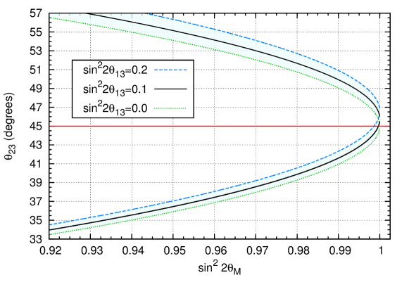
Figure 1: Allowed values for ${\theta_{23}}$ (y-axis) in degrees, for a given measurement of $\sin^{2}2\theta_{\mu\mu}$ (x-axis). The dashed (blue) and dotted (green) curves are for the extreme cases $\sin^{2}2\theta_{13}=0.2$ and $0.0$, respectively. The solid (black) curve is for $\sin^{2}2\theta_{13}=0.1$.

The main point to be noted here is the asymmetry of the band about the ${\theta_{23}}=45^{\circ}$ line. When $\sin^{2}2\theta_{13}=0$, we see that the curve is symmetric about ${\theta_{23}}=45^{\circ}$. However, for larger values of ${\theta_{13}}$ such as $\sin^{2}2\theta_{13}=0.2$, we lose this symmetry. For instance, if $\sin^{2}2\theta_{13}=0.2$ and if the MINOS measured value of $\sin^{2}2\theta_{\mu\mu}=0.98$, then the values of ${\theta_{23}}$ in the two octants are $40.5^{\circ}$ and $52.7^{\circ}$. These two angles are not complementary. In other words, it is $\theta_{\mu\mu}$ that goes to $90-\theta_{\mu\mu}$ under the octant degeneracy; but ${\theta_{23}^{LO}}$ and ${\theta_{23}^{HO}}$ are not complementary angles - the exact change depends on the value of ${\theta_{13}}$. Henceforth, for convenience, we will refer to ${\theta_{23}^{LO}}$ and ${\theta_{23}^{HO}}$ corresponding to a given measurement of $\sin^{2}2\theta_{\mu\mu}$ as being $\mu$-complementary .

As an interesting aside, we note that (given $\sin^{2}2\theta_{13}=0.1$) if $44.3^{\circ}<\theta_{\mu\mu}<45.7^{\circ}$, i.e. if $\sin^{2}2\theta_{\mu\mu}>0.9993$, then both allowed values of ${\theta_{23}}$ are greater than $45^{\circ}$. In such a case, there is no ambiguity in the octant of ${\theta_{23}}$ – it is necessarily in the higher octant. However, current experiments do not have the precision to distinguish $\sin^{2}2\theta_{\mu\mu}=0.9993$ from $\sin^{2}2\theta_{\mu\mu}=1$. Therefore, this point is purely of academic interest.

Hereafter, we assume that $\sin^{2}2\theta_{13}=0.1$. When $\sin^{2}2\theta_{\mu\mu}=1.0$, i.e. $\theta_{\mu\mu}^{LO}=\theta_{\mu\mu}^{HO}=45^{\circ}$, we get ${\theta_{23}^{LO}}={\theta_{23}^{HO}}=45.75^{\circ}$ from Eq. 10. This is also seen from Fig. 1. For a given value of $\sin^{2}2\theta_{\mu\mu}\neq 1.0$, the two allowed values of $\theta_{\mu\mu}$ have equal and opposite deviations from $45^{\circ}$, i.e. $\theta_{\mu\mu}^{LO}<45^{\circ}$ and $\theta_{\mu\mu}^{HO}>45^{\circ}$. However, the two $\mu$-complementary values of ${\theta_{23}}$ lie on opposite sides of $45.75^{\circ}$. Since

$$\sin\theta_{\mu\mu}^{LO}=\sin{\theta_{23}^{LO}}\ \cos{\theta_{13}}~{}\textrm{and}$$

$$\sin\theta_{\mu\mu}^{HO}=\cos\theta_{\mu\mu}^{LO}=\sin{\theta_{23}^{HO}}\ \cos{\theta_{13}}~{},$$

one can eliminate $\theta_{\mu\mu}^{LO}$ between these two equations. This gives us

$$\sin{\theta_{23}^{HO}}=\sqrt{\frac{1}{\cos^{2}{\theta_{13}}}-\sin^{2}{\theta_{23}^{LO}}}~{},$$ (11)

which is a handy equation to switch from one octant to another. For example, if ${\theta_{23}^{LO}}=40^{\circ}$, this equation tells us that the corresponding value of ${\theta_{23}^{HO}}$ is $51.54^{\circ}$.

We can try to recast Eq. 11 in terms of deviations from maximality, rather than in terms of the angles themselves. To this end, we define

$$\delta_{23}^{LO/HO}={\theta_{23}}^{LO/HO}-45^{\circ}~{}.$$

Assuming small deviations, we can linearize Eq. 11. This gives us

$$\delta_{23}^{HO}=\tan^{2}{\theta_{13}}-\delta_{23}^{LO}\approx 1.5^{\circ}-\delta_{23}^{LO}~{},$$ (12)

which implies

$${\theta_{23}^{HO}}=91.5^{\circ}-{\theta_{23}^{LO}}~{}.$$ (13)

We will use these relations to interpret the results of our simulations.

In Ref. Minakata et al. (2004), the authors have argued that a precise measurement of ${\theta_{23}}$ is difficult in the vicinity of $45^{\circ}$ because $\sin^{2}2\theta_{23}$ attains a maximum here, making $\Delta(\sin^{2}2\theta_{23})$ very small. Therefore it is worth discussing whether this ${\theta_{13}}$-effect can have experimentally observable consequences. In order to directly observe a shift of $0.75^{\circ}$ at $\theta_{\mu\mu}=45^{\circ}({\theta_{23}}=45.75^{\circ})$, we need a precision of $0.001$ in our measurement of $\sin^{2}2\theta_{23}$. This is far beyond our experimental reach. However, if $\theta_{\mu\mu}^{LO}=40^{\circ}({\theta_{23}^{LO}}=40.63^{\circ})$, the precision in $\sin^{2}2\theta_{23}$ required to observe this shift is around $0.007$, which may be achievable at future facilites. Moreover, this effect can be felt indirectly, as an artificially enhanced/reduced sensitivity in oscillation experiments. We illustrate this through simulations, in the next section.

III Simulations

As we have mentioned before, our aim is to illustrate the difference between choosing the ‘wrong’ definition: ${\theta_{23}}=\theta_{\mu\mu}$ and the ‘right’ definition: ${\theta_{23}}=\sin^{-1}(\sin\theta_{\mu\mu}/\cos{\theta_{13}})$. In order to show the experimentally observable effects of this choice, we have simulated the NO$\nu$A experiment using the GLoBES package Ayres et al. (2007); Huber et al. (2005, 2007); Yang and Wojcicki (2004); Messier (1999); Paschos and Yu (2002); Patterson (2012). In this section, we discuss the results of our simulations.

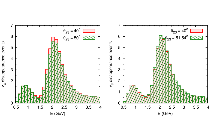
Figure 2: $\nu_{\mu}$ disappearance event rates for ${\theta_{23}^{LO}}=40^{\circ}$ are shown as a solid (red) histogram in both panels. Superimposed on this, as a hatched (green) histogram are the event rates for the corresponding ${\theta_{23}^{HO}}$ using the ‘wrong’ definition (left panel) and ‘right’ definition (right panel). For the ‘right’ definition, the event rates show a good match.

We have used the standard NO$\nu$A setup Ayres et al. (2007), with a 14 kton totally active scintillator detector placed 810 km away from the NuMI beam at a 14 mrad off-axis location. The beam, with a power of 0.7 MW, is assumed to run for three years each with neutrinos and antineutrinos. We have taken the energy resolution for $\nu_{\mu}$ to be $0.06\sqrt{E\textrm{(}GeV)}$ Patterson (2012). Backgrounds from NC events have also been taken into account. For the oscillation parameters, we have chosen $\sin^{2}{\theta_{12}}=0.304$, $\sin^{2}2{\theta_{13}}=0.1$, ${\Delta_{21}}=7.6\times 10^{-5}\ \textrm{eV}^{2}$, $\Delta_{\mu\mu}=2.4\times 10^{-3}\ \textrm{eV}^{2}$ and ${\delta_{CP}}=0$, unless specified otherwise.

In Fig. 2, we have plotted the event rates from the muon disappearance channel. In the left panel, we have chosen the ‘wrong’ definition of ${\theta_{23}}$, so that ${\theta_{23}^{LO}}=40^{\circ}$ implies ${\theta_{23}^{HO}}=50^{\circ}$. This gives us a difference in the number of events. However, on using the ‘right’ definition (${\theta_{23}^{HO}}=51.54^{\circ}$), we find that the event rates match, as seen in the right panel.

Having showed the difference due to our choice of ${\theta_{23}}$ at the event level, we now proceed to do so at the level of ${\chi^{2}}$. Throughout our simulations, we have used the values specified above as the true values of oscillation parameters. We have varied the test values of the parameters in the following ranges: $\sin^{2}2\theta_{13}\in[0.07,0.13]$, $\theta_{\mu\mu}\in[35^{\circ},55^{\circ}]$, $|\Delta_{\mu\mu}|\in[2.05,2.75]\times 10^{-3}\ \textrm{eV}^{2}$ and ${\delta_{CP}}\in[0,2\pi)$. The solar parameters ${\Delta_{21}}$ and ${\theta_{12}}$ have been kept fixed in this analysis, since the effect of their variation is small. The mass hierarchy is assumed to be normal.

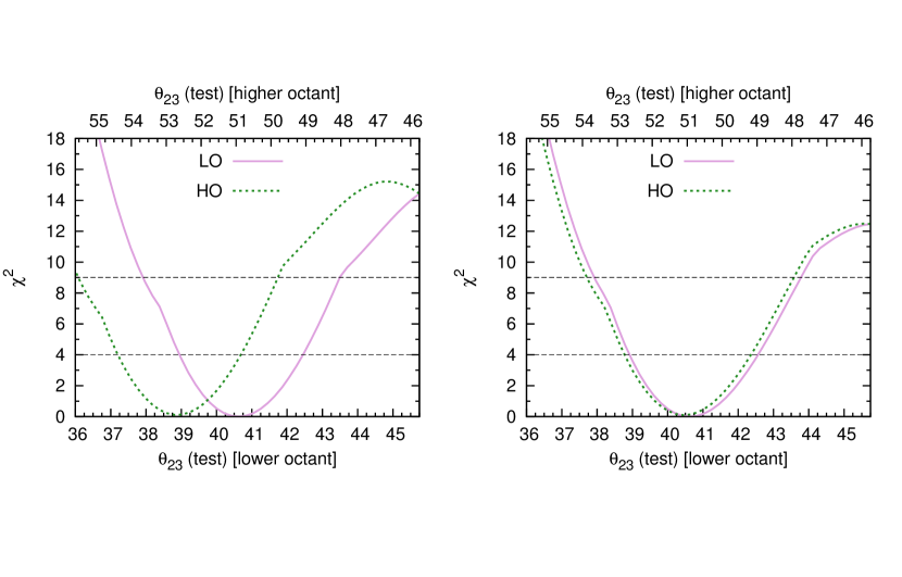
Figure 3: ${\chi^{2}}$ for sensitivity to the value of ${\theta_{23}}$ from muon disappearance from NO$\nu$A . True $\theta_{\mu\mu}=40^{\circ}$. The solid (pink) curve gives ${\chi^{2}}$ for test $\theta_{\mu\mu}$ in the lower octant (read the lower x-axis), wile the dotted (green) curve gives ${\chi^{2}}$ for test $\theta_{\mu\mu}$ in the higher octant (read the upper x-axis). In the left panel, we have chosen the ‘wrong’ definition of ${\theta_{23}}$ while in the right panel we have chosen the ‘right’ definition of ${\theta_{23}}$.

In Fig. 3, we have plotted the sensitivity to ${\theta_{23}}$ for true $\theta_{\mu\mu}=40^{\circ}$. As the test value of $\theta_{\mu\mu}^{LO}$ increases in the lower (true) octant from $35^{\circ}$ to $45^{\circ}$, ${\theta_{23}^{LO}}$ increases from $35.53^{\circ}$ to $45.75^{\circ}$. This range is shown on the lower x-axis. Correspondingly, ${\theta_{23}^{HO}}$ decreases from $55.60^{\circ}$ to $45.75^{\circ}$. This range, for the higher (false or degenerate) octant, is shown on the upper x-axis. The advantage of using these double-axes is that values of ${\theta_{23}}$ along a vertical line are $\mu$-complementary . We have used the linearized relation in Eq. 13 to plot these axes. For values of test $\theta_{\mu\mu}$ in the lower octant, ${\chi^{2}}$ has been plotted as the solid (pink) curve. The lower x-axis should be used to read the ${\theta_{23}}$ values for this curve. For values of test $\theta_{\mu\mu}$ in the higher octant, ${\chi^{2}}$ has been plotted as the dotted (green) curve. The upper x-axis should be used to read the ${\theta_{23}}$ values for this curve.

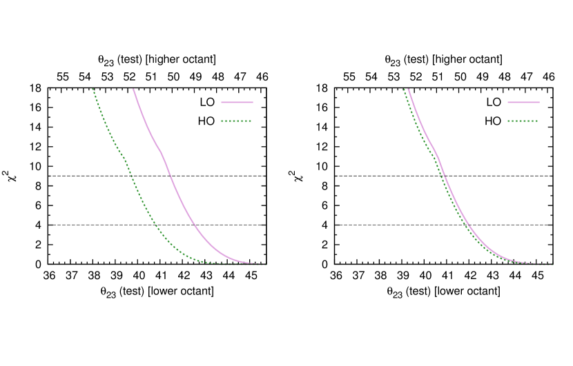
Figure 4: ${\chi^{2}}$ for sensitivity to the value of ${\theta_{23}}$ from muon disappearance from NO$\nu$A . True $\theta_{\mu\mu}=45^{\circ}$. The solid (pink) curve gives ${\chi^{2}}$ for test $\theta_{\mu\mu}$ in the lower octant (read the lower x-axis), wile the dotted (green) curve gives ${\chi^{2}}$ for test $\theta_{\mu\mu}$ in the higher octant (read the upper x-axis). In the left panel, we have chosen the ‘wrong’ definition of ${\theta_{23}}$ while in the right panel we have chosen the ‘right’ definition of ${\theta_{23}}$.

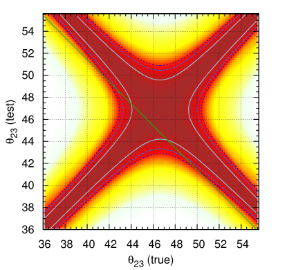
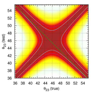
Figure 5: Allowed test values for ${\theta_{23}}$ (y-axis) in degrees, for a given true value of ${\theta_{23}}$ (x-axis). $68\%$, $90\%$ and $95\%$ C.L. contours are also shown. As before, the left(right) panel is plotted using the ‘wrong(right)’ definition of ${\theta_{23}}$. With the ‘right’ definition, we see the expected behaviour - the false degenerate solution lies along the line ${\theta_{23}^{HO}}=91.5^{\circ}-{\theta_{23}^{LO}}$ (shown by the straight diagonal (green) line).

The following features are visible in Fig. 3: (a) For $\theta_{\mu\mu}=40^{\circ}$, the best-fit point is seen at the corresponding value of ${\theta_{23}}$ which is $40.63^{\circ}$ (b) If we use the ‘wrong’ definition of ${\theta_{23}}$, the minima in the two octants do not appear for $\mu$-complementary values of ${\theta_{23}}$. This is seen in the left panel. In the right panel, we have used the ‘right’ definition. As a result, we find that the minima coincide. (c) The sensitivities in the two octants coincide at ${\theta_{23}}=45.75^{\circ}$, rather than ${\theta_{23}}=45^{\circ}$. This is expected from the analytic calculations presented in the previous section.

Figure 4 is similar to Fig. 3, but with true $\theta_{\mu\mu}=45^{\circ}$. Note that compared to the ‘right’ definition ${\chi^{2}}$, the ‘wrong’ definition ${\chi^{2}}$ is more in the lower octant, and less in the higher octant. Clearly, using the ‘wrong’ definition gives us an incorrect value of ${\chi^{2}}$. Thus, if ${\chi^{2}}$ from the ‘wrong’ definition is used to set a prior on ${\theta_{23}}$ for future experiments, it will give a spurious indication of the confidence with which certain ${\theta_{23}}$ values are allowed. This also has implications for octant sensitivity studies. Since ${\theta_{23}}$ and $90^{\circ}-{\theta_{23}}$ are not $\mu$-complementary ​, ${\chi^{2}}({\theta_{23}};90^{\circ}-{\theta_{23}})$ does not give the correct octant sensitivity. Therefore, care must be taken to use the ‘right’ definition in simulations.

Finally, in Fig. 5, we have plotted the allowed values of ${\theta_{23}}$ for all possible true values of ${\theta_{23}}$ in the range $[36^{\circ},55^{\circ}]$. For each true value, the allowed test values can be read from its corresponding vertical line. The $68\%$, $90\%$ and $95\%$ C.L. contours are also shown. For a given true value of ${\theta_{23}}$, we find an allowed range of test ${\theta_{23}}$ in each octant. For the ‘right’ definition, we see that the false degenerate solution lies along the line ${\theta_{23}^{HO}}=91.5^{\circ}-{\theta_{23}^{LO}}$ (Eq. 13). But if we choose the ‘wrong’ definition, then we get degenerate solutions that are not $\mu$-complementary , along with incorrect values of ${\chi^{2}}$.

In this paper, we have only presented the results for the case where NH is the true hierarchy, and true ${\delta_{CP}}=0$. However, we have verified that these results hold for IH, and for a number of values of ${\delta_{CP}}$.

IV Conclusions and Summary

In this study, we have discussed the effect of three-flavour mixing on our measurement of ${\theta_{23}}$. We have calculated the relation between the value of ${\theta_{23}}$ in nature, and $\theta_{\mu\mu}$ that is measured in muon disappearance experiments. The difference between these two numbers is significant, in light of the measured value of ${\theta_{13}}$. Using the ‘right’ definition of ${\theta_{23}}$ (incorporating the ${\theta_{13}}$-effect), we have found the allowed values of ${\theta_{23}}$ in the two octants, corresponding to a single measured value of $\sin^{2}2\theta_{\mu\mu}$. We know that complementary values of $\theta_{\mu\mu}$ in the two octants are related by $\theta_{\mu\mu}^{HO}=90^{\circ}-\theta_{\mu\mu}^{LO}$. But for a given measurement of $\sin^{2}2\theta_{\mu\mu}$, we have found that the corresponding values of ${\theta_{23}}$ in the two octants are related by ${\theta_{23}^{HO}}=91.5^{\circ}-{\theta_{23}^{LO}}$. We have called this relation $\mu$-complementarity. The exact form of this equation comes from the value of ${\theta_{13}}$.

Through simulations, we have showed that using the ‘wrong’ definition gives us degenerate fits at non-$\mu$-complementary values of ${\theta_{23}}$. Consequently, the muon disappearance analysis can give an incorrect prior on ${\theta_{23}}$. In determining octant sensitivity, if the ‘wrong’ definition is used, one can get an incorrect value of ${\chi^{2}}$. Therefore, we advocate the use of the ‘right’ definition (as given in Eq. 10) for calculating the oscillation probability in simulations. However, priors from previous experiments should be added in terms of $\sin^{2}2\theta_{\mu\mu}$ – the quantity that is measured in the muon disappearance experiments. Our results and conclusions have been found to hold true for both hierarchies and for values of ${\delta_{CP}}$ in its entire allowed range.