Determination of $\theta_{23}$ in Long-Baseline Neutrino Oscillation Experiments with Three-Flavor Mixing Effects

Abstract

We examine accuracy of $\theta_{23}$ determination in future long-baseline (LBL) $\nu_{\mu}$ disappearance experiments in the three-flavor mixing scheme of neutrinos. Despite that the error of $\sin^{2}{2\theta_{23}}$ is indeed a few% level at around the maximal mixing, we show that the error of physics variable $s^{2}_{23}$ is large, $\delta(s^{2}_{23})/s^{2}_{23}\simeq 10\mbox{-}20\%$, depending upon regions of $\theta_{23}$. The errors are severely affected by the octant degeneracy of $\theta_{23}$, and $\delta(s^{2}_{23})$ is largely amplified by the Jacobian factor relating these two variables in a region near to the maximal mixing. The errors are also affected by the uncertainty due to unknown value of $\theta_{13}$; $\delta(s^{2}_{23})$ is doubled at off maximal in the second octant of $\theta_{23}$ where the effect is largest. To overcome this problem, we discuss combined analysis with $\nu_{e}$ appearance measurement in LBL experiments, or with reactor measurement of $\theta_{13}$. For possible relevance of sub-leading effects even in the next-generation LBL experiments, we give a self-contained derivation of the survival probability to the next to leading order in $s^{2}_{13}$ and $\Delta m^{2}_{21}/\Delta m^{2}_{31}$.

I Introduction

At several years since the pioneering discovery in atmospheric neutrino observation by Super-Kamiokande (SK) SKatm , we now have compelling evidences for neutrino oscillation. The direct confirmation of oscillation of atmospheric neutrinos comes from the K2K experiment using man-made neutrino beam K2K which confirmed its existence at 3.9$\sigma$ CL K2K_new . The neutrino oscillation with the solar $\Delta m^{2}$ scale is beautifully observed by the KamLAND experiment KamLAND ; KamLAND_new . By observing deficit in reactor antineutrino flux it pinned down the large-mixing-angle (LMA) solution of the solar neutrino problem based on the Mikheyev-Smirnov-Wolfenstein (MSW) mechanism wolfenstein ; MSW . It has thereby settled the long-standing solar neutrino problem BD , whose origin was identified as due to the neutrino flavor transformation by SNO SNO . Long awaited confirmation of the oscillatory behavior is now available by the three experiments, SK SKatm_new , K2K K2K_new , and KamLAND KamLAND_new . Thus, we already know roughly the structure of lepton flavor mixing in the (1-2) and (2-3) sectors of the Maki-Nakagawa-Sakata (MNS) matrix MNS .

We recognize that there are two small (or possibly vanishing) quantities in the lepton mixing matrix, $\theta_{13}$ and deviation of $\theta_{23}$ from $\pi/4$. The former is constrained mainly by the reactor experiments CHOOZ to be $\sin^{2}{2\theta_{13}}\leq 0.15$ at 90% CL by a global analysis global , while the latter is bounded as $0\leq 1-\sin^{2}{2\theta_{23}}\leq 0.08$ at 90% CL by the recent reanalysis of atmospheric neutrino data by the SK group kearns . Possible correlation between these two small quantities may imply hints for the yet unknown discipline that was used by nature to design the structure of lepton flavor mixing. Some symmetries have been discussed by which the maximal $\theta_{23}$ is correlated with vanishing $\theta_{13}$ in the symmetry limit symmetry . Furthermore, the question of how large is the deviation of $\theta_{23}$ from $\pi/4$ is discussed from a variety of viewpoints deviation . Therefore, it is important to determine the value of not only $\theta_{13}$ but also $\theta_{23}$ very precisely.

How accurately $\theta_{23}$ can be measured experimentally? It appears that measurement of disappearance probability of $\nu_{\mu}$ at around the first oscillation maximum has highest sensitivity to $\sin^{2}{2\theta_{23}}$. In the J-PARC $\rightarrow$ Super-Kamiokande (JPARC-SK) experiment, for example, $\sin^{2}{2\theta_{23}}$ is expected to be determined to 1% accuracies JPARC . Given such an enormous accuracy, it seems that there is not much to add because it looks like the best thinkable accuracy of mixing angle determination in neutrino experiments. Unfortunately, it is not quite true. We discuss three relevant and mutually related issues in this paper which prevent an accurate determination of $\theta_{23}$, in particular, its small deviation from the maximal. The points we discuss are:

• a large Jacobian associated with transformation of the variable from $\sin^{2}{2\theta_{23}}$ to $s^{2}_{23}$ at around the maximal mixing

• the octant ambiguity of $\theta_{23}$ (two solutions of $\theta_{23}$ larger or smaller than $\pi/4$)

• effects of three-flavor mixing, in particular of non-vanishing $\theta_{13}$

While the first point is “kinematical” in nature, the second and the third points reflect the three-flavor structure of lepton mixing. Although each of these points was discussed in various occasions in the past, we believe that they are never discussed in a coherent fashion in the context of precision measurement of $\theta_{23}$ by long-baseline (LBL) experiments. The estimation of errors of $\theta_{23}$ determination is also done by taking account of three-flavor mixing effects AHKSW ; munich10 with consistent results with ours. Yet, they offer neither understanding of the reasons behind the estimated large errors in the similar depth as we provide, nor ways of improvement by combining with e.g., reactor measurement.

Importance of experimental determination of $\theta_{13}$ is now well recognized in the community by itself and as a door to exploration of leptonic CP violation. Strategies for determining the remaining oscillation parameters are developed with use of accelerator superbeam superbeam and reactor neutrinos MSYIS , which followed by a series of feasible experimental programs JPARC ; NuMI ; SPL ; reactor_white . The accuracies of $\theta_{13}$ determination in the LBL and the reactor experiments are expected to reach to $\sin^{2}{\theta_{13}}\simeq 2.5\times 10^{-3}$. We feel that the strategy for similar accurate determination of $\theta_{23}$ is relatively less well developed, and it is the purpose of this paper to trigger such efforts.

By indicating that the three-flavor nature of the oscillation probability already manifests itself in the next generation LBL experiments, our discussion in this paper might have an implication to future neutrino oscillation research, suggesting a possible direction. The next to leading order corrections may be important due to the larger ratio of $\epsilon\equiv\Delta m^{2}_{21}/\Delta m^{2}_{31}\simeq 1/30$ due to a larger $\Delta m^{2}_{21}$ KamLAND_new , and possible large value of $\theta_{13}$ close to the CHOOZ bound. Under such hope, we present in Appendix A a derivation of the full expression of survival probability $P(\nu_{\mu}\rightarrow\nu_{\mu})$ to the next to leading order in $\epsilon$ and $s^{2}_{13}$, which is used in our analyses throughout this paper. See also perturbative for derivation of such formulas under the similar spirit.

II Why is accurate determination of $\theta_{23}$ so difficult?

In this section we present pedagogical description of the three reasons for difficulty of accurate determination of $\theta_{23}$ that were mentioned in Sec. I. The readers who are familiar to them are advised to skip this section and go directly to Sec. III.

II.1 Problems of large Jacobian at around the maximal mixing

The ultimate purpose of the whole experimental activities which aim at measuring neutrino mixing parameters is to understand physics of lepton flavor mixing. For this purpose precise determination of the angles or the sine of angles are required.

The $\nu_{\mu}$ disappearance measurement is sensitive to $\sin^{2}{2\theta_{23}}$, not $s^{2}_{23}$, which is unfortunate, but is actually the case. It inherently makes accuracy of determination of $\theta_{23}$ much worse than it is achieved for $\sin^{2}{2\theta_{23}}$ at around the maximal mixing. Assuming that the true value of $\theta_{23}$ is $\pi/4$, for example, an accurate measurement of $\sin^{2}{2\theta_{23}}$ with error of 1% level translates into large error of $\pm 10$% level for $s^{2}_{23}$. It is simply because the Jacobian for the transformation of the variables

$$\frac{\delta(s_{23}^{2})}{\delta(\sin^{2}{2\theta_{23}})}\simeq\frac{ds^{2}_{23}}{d\sin^{2}{2\theta_{23}}}=\frac{1}{4\cos{2\theta_{23}}},$$ (1)

are large at around $\theta_{23}=\pi/4$, by which a tiny error obtained for $\sin^{2}{2\theta_{23}}$, denoted as $\delta(\sin^{2}{2\theta_{23}})$ in (1), can be translated into a large error $\delta(s_{23}^{2})$ for $s_{23}^{2}$. It is what happens in Fig. 3 in Sec. III.

We emphasize that use of $s^{2}_{23}$, not $\sin^{2}{2\theta_{23}}$, is inevitable in the error analysis based on three flavor mixing because the $\nu_{\mu}$ survival probability itself cannot be expressed in terms of $\sin^{2}{2\theta_{23}}$ only once next to the leading order correction is taken into account. See (6) below and (29) for the probabilities in vacuum and in matter, respectively. It is even more so if we combine $\nu_{e}$ appearance measurement into our analysis, as will be done in Sec. IV, because the dominant term in the $\nu_{e}$ appearance probability depends upon $\theta_{23}$ through $s^{2}_{23}$.

II.2 Octant ambiguity of $\theta_{23}$

The dominant term in $\nu_{\mu}$ survival probability, and hence the disappearance measurement, is sensitive primarily to $\sin^{2}{2\theta_{23}}$. Therefore, there exist two solutions of $\theta_{23}$ for a given value of the survival probability $P(\nu_{\mu}\rightarrow\nu_{\mu})$, the octant ambiguity of $\theta_{23}$. In Fig. 1 we present a contour of 90% CL allowed region in $s^{2}_{23}\mbox{-}s^{2}_{13}$ space by 5 years measurement at JPARC-SK based on the analysis in Sec. III whose details will be explained in Appendix B.

It should be noticed in Fig. 1 that there exist “clone” solutions, which arise as a consequence of the degeneracy of $\theta_{23}$ solutions octant . Namely, with an assumed true value $s^{2}_{23}=0.34$, for example, the measurement allows two regions as solutions, one around the original value of $s_{23}$ in the first octant and the other one around $s^{2}_{23}=0.66$ which is the reflected point with respect to $\theta_{23}=\pi/4$ in the second octant. Of course, it does not produce additional experimental error of $s^{2}_{23}$ as far as two regions are separated, though ambiguity exists of which region contains the true value of $\theta_{23}$. But once the two allowed regions start to merge (which takes place near the maximal $\theta_{23}$), it does produce additional error of $s^{2}_{23}$ as exhibited in the spike in Fig. 3. The similar figure as Fig. 1 indicating $\theta_{23}\mbox{-}\theta_{13}$ correlation and clone solution is used in a slightly different context in gab-gouvea .

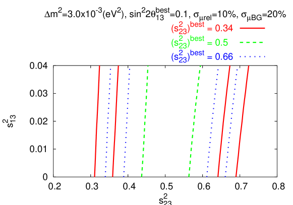
Figure 1: 90% CL allowed regions are plotted in $s^{2}_{23}\mbox{-}s^{2}_{13}$ space by assuming that the best fit values given by nature are [$(s_{23}^{2})^{\text{best}}$, $(s_{13}^{2})^{\text{best}}$] = [0.34, 0.026] (red solid curve), [0.5, 0.026] (green dashed curve), and [0.66, 0.026] (blue dotted curve); Note that $s_{23}^{2}=0.34$ and 0.66 correspond to $\sin^{2}{2\theta_{23}}=0.9$ which is the lowest edge of the current allowed region and $s_{13}^{2}=0.026$ corresponds to $\sin^{2}{2\theta_{13}}=0.1$. The systematic errors are assumed to be ($\sigma_{\mu{\text{rel}}}$, $\sigma_{{\mu\text{BG}}}$) = (10%, 20%).

II.3 Three-flavor mixing effects in the disappearance measurement of $\theta_{23}$

While the effect of three-flavor mixing gives relatively mild influence to the accuracy of $\theta_{23}$ measurement compared to the above two effects, it is nonetheless non-negligible. Let us explain the key point by taking a very simple case using the approximation of vacuum oscillation and small deviation from maximality of $\theta_{23}$. Though simplified, the model captures some relevant features possessed by the more realistic cases.

We use, throughout this paper, the standard notation of the MNS matrix PDG ,

$$U=\left[\begin{array}[]{ccc}c_{12}c_{13}&s_{12}c_{13}&s_{13}e^{-i\delta}\\ -s_{12}c_{23}-c_{12}s_{23}s_{13}e^{i\delta}&c_{12}c_{23}-s_{12}s_{23}s_{13}e^{i\delta}&s_{23}c_{13}\\ s_{12}s_{23}-c_{12}c_{23}s_{13}e^{i\delta}&-c_{12}s_{23}-s_{12}c_{23}s_{13}e^{i\delta}&c_{23}c_{13}\\ \end{array}\right],$$ (5)

where $c_{ij}$ and $s_{ij}$ ($i,j=1\mbox{-}3$) imply $\cos{\theta_{ij}}$ and $\sin{\theta_{ij}}$, respectively. The mass squared difference of neutrinos is defined as $\Delta m^{2}_{ij}\equiv m^{2}_{i}-m^{2}_{j}$ where $m_{i}$ is the eigenvalue of the $i$th mass-eigenstate. Then, the disappearance probability $1-P(\nu_{\mu}\rightarrow\nu_{\mu})$ in vacuum is given by

$$1-P(\nu_{\mu}\rightarrow\nu_{\mu}) = \sin^{2}2\theta_{23}\sin^{2}\Bigl{(}\frac{\Delta m^{2}_{31}L}{4E}\Bigr{)}+4s_{13}^{2}s_{23}^{2}(s_{23}^{2}-c_{23}^{2})\sin^{2}\Bigl{(}\frac{\Delta m^{2}_{31}L}{4E}\Bigr{)}$$ (6)

$$- c_{12}^{2}\sin^{2}2\theta_{23}\Bigl{(}\frac{\Delta m_{21}^{2}L}{4E}\Bigr{)}\sin\Bigl{(}\frac{\Delta m_{31}^{2}L}{2E}\Bigr{)}.$$

In the right-hand side of (6), the first term represents major contribution which survives in the two-flavor or the single mass-scale dominance approximation one-mass . The second and the third terms are small corrections due to non-vanishing $s^{2}_{13}$ and $\epsilon\equiv\Delta m^{2}_{21}/\Delta m^{2}_{31}$, respectively, which give effects of the three-flavor mixing. It is obvious that the second term vanishes for the maximal $\theta_{23}$, while the third term vanishes at the oscillation maximum, $\Delta m_{31}^{2}L/2E=\pi$.

Suppose that we perform a hypothetical experiment at a monochromatic energy close (but not identical) to the oscillation maximum, $\sin{(\Delta m_{31}^{2}L/2E)}\ll 1$. We assume that deviation from maximality of $\theta_{23}$ is small, and parametrize it by $\eta$ defined as $\eta\equiv\cos{2\theta_{23}}$ (so that $1-\sin^{2}{2\theta_{23}}=\eta^{2}\ll 1$). Using the approximation $\sin{(\Delta m_{31}^{2}L/4E)}=1$ we obtain

$$P(\nu_{\mu}\rightarrow\nu_{\mu})=\eta(\eta+2s^{2}_{13})+\frac{\pi}{2}c^{2}_{12}\epsilon\sin\left(\frac{\Delta m^{2}_{31}L}{2E}\right).$$ (7)

Notice that the linear term in $\eta$ in (7) distinguishes between $\theta_{23}$ in the first and the second octants because $\eta$ changes sign depending upon which octant it lives. The equation (7) clearly indicates that the larger value of $s_{13}^{2}$ gives the smaller (larger) value of $\eta$ in first (second) octant of $\theta_{23}$ for a given $P(\nu_{\mu}\to\nu_{\mu})$. It is interesting to observe that the feature of $\theta_{23}$-$\theta_{13}$ correlation is in fact shared in Fig. 1.

Therefore, what the disappearance measurement actually determines is not $\sin^{2}{2\theta_{23}}$ but allowed regions in $s^{2}_{23}\mbox{-}s^{2}_{13}$ space. The feature leads to larger errors of $\theta_{23}$ in three-flavor analysis compared to those of two-flavor analysis. It is notable that the effect of $s_{13}^{2}$ is slightly more significant in the second octant of $\theta_{23}$. Note also the tendency of departure from the maximal $\theta_{23}$ due to $\theta_{13}$ is smaller (larger) at larger $\theta_{13}$ in the first (second) octant of $\theta_{23}$. These properties are the key to fuller understanding of the features of the errors of $\theta_{23}$ to be discussed in the next section. The problem of $\theta_{13}$ dependence of accuracy of $\theta_{23}$ determination has been addressed, e.g., in barger_etal .

Another notable feature in (7) is that the solar mass scale correction can come into play a role. It can change the depth of the dip of $P(\nu_{\mu}\rightarrow\nu_{\mu})$ and therefore may affect the value of $\eta$.

III Disappearance measurement of $\theta_{23}$ and three-flavor mixing effect

In this section, we fully analyze the sensitivity of $\theta_{23}$ by $\nu_{\mu}$ disappearance measurement by taking account of the three-flavor mixing effects. To make our discussion as concrete as possible, we take the particular experiment, the JPARC-SK experiment JPARC . While the Jacobian and the degeneracy effects are universal to any experiments, the three-favor effect is most prominent if the systematic uncertainties of the experiment are small enough to allow measurement of $\sin^{2}{2\theta_{23}}$ to a few % level accuracies. We describe in detail the statistical method used in our analysis in Appendices B and C so that we can concentrate on physics discussion in the main text. Through the course of formulating our analysis procedure, we will try to reproduce the results of sensitivity analyses by the experimental group. (See Fig. 5.)

We take 22.5 kt as the fiducial volume of SK and assume, throughout this paper, 5 years running of neutrino mode $\nu_{\mu}$ disappearance measurement, as expected in its phase I defined in LOI. We examine two cases of systematic errors, ($\sigma_{\mu{\text{rel}}}$, $\sigma_{{\mu\text{BG}}}$) = (10%, 20%) and (5%, 10%). The former numbers, which are based on their experience in K2K, can be too pessimistic but are quoted in LOI, while the latter may be a reasonable goal to be reached in phase I of the J-PARC neutrino project. To make the goal and to achieve even smaller errors the group plans to build an intermediate detector at $\sim$ 2km from J-PARC. We use, unless otherwise stated, $\Delta m_{31}^{2}=3\times 10^{-3}$eV², $\Delta m_{21}^{2}=7.3\times 10^{-5}$eV² and $s_{12}^{2}=0.315$. We take the earth matter density $\rho=2.3\,\mbox{g}\cdot\mbox{cm}^{-3}$ based on the estimation quoted in koike-sato .

We assume that $\Delta m^{2}_{31}>0$ in our analysis. We have checked that the error $\delta(\sin^{2}{2\theta_{23}})$ slightly increases in the case of negative $\Delta m^{2}_{31}$ but only by about 0.001 in the allowed region of $\theta_{23}^{\text{best}}$. In this paper, the quantity with superscript “best” always implies the best fit value given by nature. We have also checked that our results do not change in any appreciable manner by taking $\Delta m^{2}_{21}$ at the highest end of the LMA-I parameter, $\Delta m^{2}_{21}=10^{-4}\mbox{eV}^{2}$. Therefore, we do not discuss further about the possible effects caused by flipping the sign of $\Delta m^{2}_{31}$ and by raising the solar $\Delta m^{2}_{21}$.

III.1 Accuracy of determination of $s^{2}_{23}$ vs. that of $\sin^{2}{2\theta_{23}}$

We compare the accuracies of determination of $\sin^{2}{2\theta_{23}}$ and $s^{2}_{23}$ to illuminate how the problem of Jacobian and the degeneracy affect the accuracy of $\theta_{23}$ determination. We show in Fig. 2 the errors expected for determination of $\sin^{2}{2\theta_{23}}$ as a function of $\sin^{2}{2\theta_{23}^{\text{best}}}$. In Fig. 2a and Fig. 2b, the systematic errors are taken as ($\sigma_{\mu{\text{rel}}}$, $\sigma_{{\mu\text{BG}}}$) = (10%, 20%) and (5%, 10%), respectively. The figure includes not only the result of the three-flavor analysis with the particular nonzero input value of $\theta_{13}$, $\sin^{2}{2\theta_{13}^{\text{best}}}=0.1$, but also that of the two-flavor analysis assuming $\theta_{13}=\theta_{13}^{\text{best}}=0$. We note that the results depend on input values of $\theta_{13}^{\text{best}}$ but only mildly; If we take $\sin^{2}{2\theta_{13}^{\text{best}}}=0$ in the three flavor analysis, the uncertainty of $\sin^{2}{2\theta_{23}}$ decreases only by $\sim$5%.

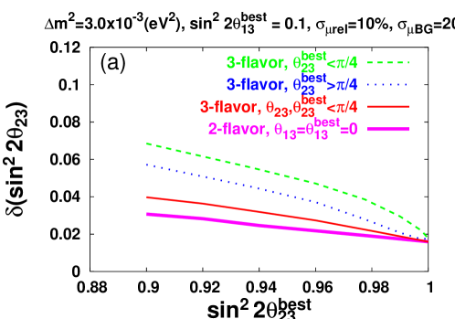
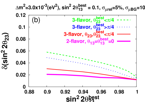
Figure 2: The expected accuracies of determination of $\sin^{2}{2\theta_{23}}$ at 90% CL obtained by the three-flavor analysis are compared with that of our two-flavor analysis ($\theta_{13}=\theta_{13}^{\text{best}}=0$) which is indicated by pink thick-solid line. The red thin-solid line is the result obtained in the analysis assuming that the $\theta_{23}$ is in the first octant, $0\leq\theta_{23}\leq\pi/4$. The green dashed and blue dotted lines are for input values of $\theta_{23}^{\text{best}}$ in the first and the second octants, respectively, while allowing the output $\theta_{23}$ in the full range, $0\leq\theta_{23}\leq\pi/2$. Fig. 2a and 2b are with systematic errors ($\sigma_{\mu{\text{rel}}}$, $\sigma_{{\mu\text{BG}}}$) = (10%, 20%) and (5%, 10%), respectively.

We call special attention to the distinction between the lower solid lines, and the upper dashed and dotted lines in the three-flavor results in Fig. 2. Namely, the red thin-solid and the pink thick-solid line are obtained under the assumption that $\theta_{23}$ is in the first octant, $0\leq\theta_{23}\leq\pi/4$, by which the octant degeneracy is switched off by hand. This procedure is adopted, for example, in LOI of the JPARC-SK experiment in their sensitivity estimate JPARC . Whereas for the green dashed and the blue-dotted lines, the full region $0\leq\theta_{23}\leq\pi/2$ is allowed as output, and the input value of $\theta_{23}$ is taken in the first (second) octant of $\theta_{23}$ for the green dashed (blue dotted) lines. We recognize that our ignorance of which octant $\theta_{23}$ lives makes the error of $\sin^{2}{2\theta_{23}}$ almost twice ($\sim$ 80% increase) in the optimistic (pessimistic) case of systematic errors.

In Fig. 3, the errors expected for determination of $s^{2}_{23}$ are plotted, with systematic errors ($\sigma_{\mu{\text{rel}}}$, $\sigma_{{\mu\text{BG}}}$) = (10%, 20%) and (5%, 10%) in Fig. 3a and Fig. 3b, respectively. The readers may be surprised by the difference between Fig. 2 and Fig. 3. Although they are based on exactly the same data set, the errors $\delta(s_{23}^{2})/s_{23}^{2}$ in Fig. 3 are as large as 14%-20% in the “near to the maximal” region and the shape is quite odd, which should be compared to the smooth behavior of the curves in Fig. 2. Hereafter, we use the notations “near to the maximal” and “off the maximal” regions which mean the regions of $\theta_{23}$, $|s^{2}_{23}-0.5|\leq 0.08$ and $0.08\leq|s^{2}_{23}-0.5|\leq 0.16$, respectively. There are two main reasons for such a marked difference.

(a) Jacobian effect

As explained in Sec. II.1 the Jacobian (1) makes the uncertainty of $s^{2}_{23}$ much larger than that of $\sin^{2}{2\theta_{23}}$ near the maximal mixing. It explains the feature that the uncertainty is large in region $0.45\leq s^{2}_{23}\leq 0.55$, but it does not explain the double-peaked structure in Fig. 3.

(b) Degeneracy effect

The problem of degeneracy related with $\theta_{23}$ requires a special comment. As one can see in Fig. 1, there is a clone solution for a given input value of $\theta_{23}$. We do not include the separated clone region in defining the uncertainties in $s^{2}_{23}$. We think it appropriate not to include the separate region because it is due to the problem of parameter degeneracy and is a separate issue from the uncertainty attached to experimental $s^{2}_{23}$ determination. Nevertheless, it affects the results in Fig. 3 because the genuine and the clone regions merge near the maximal mixing. Once the true and the fake regions merge there is no way to separate them. It creates a jump of $\delta(s_{23}^{2})$ at $s^{2}_{23}\simeq 0.45$ and $\simeq 0.55$ when the true value of $s^{2}_{23}$ approaches to 0.5 from above and from below, respectively, leading to the double-peaked structure in Fig. 3.

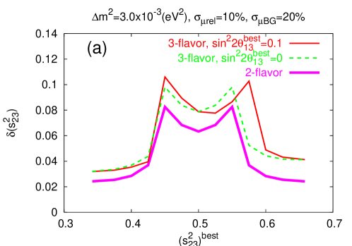
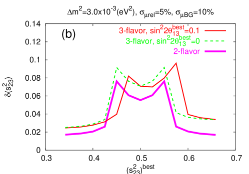
Figure 3: The expected accuracies of determination of $s_{23}^{2}$ at 90% CL obtained by the three-flavor analysis are compared with that of the two-flavor analysis ($\theta_{13}=\theta_{13}^{\text{best}}=0$) which is indicated by pink thick-solid line. The red thin-solid and green dashed lines are for input values of $\theta_{13}$ as $\sin^{2}{2\theta_{13}^{\text{best}}}=0.1$ and $\sin^{2}{2\theta_{13}^{\text{best}}}=0.0$, respectively. Fig. 3a and 3b are with systematic errors ($\sigma_{\mu{\text{rel}}}$, $\sigma_{{\mu\text{BG}}}$) = (10%, 20%) and (5%, 10%), respectively.

Notice that the sensitivity curves in Fig. 2 obtained not only with but also without the restriction $0\leq\theta_{23}\leq\pi/4$ do not have the similar jump. It is because in the analysis of error defined in terms of the variable $\sin^{2}{2\theta_{23}}$ the true and the fake regions start to overlap at even larger deviation from the maximal value of $\theta_{23}$, leading to a smooth behavior. It stems from the fact that the variable $\sin^{2}{2\theta_{23}}$ cannot distinguish between the first and the second octants, through which the confusion due to $\theta_{23}$ ambiguity is maximally enhanced. It also implies that use of the variable $\sin^{2}{2\theta_{23}}$ in defining errors leads to larger errors in regions where $\delta(s^{2}_{23})$ jumps down in Fig. 3. We emphasize again that one has to use the variable $s^{2}_{23}$ to represent uncertainty in $\theta_{23}$ determination because, in addition to the one mentioned just above, the angle is defined in the entire quadrant and the obtained uncertainties are different in the first and in the second octants.

From Fig. 3 we also observe the following features.

(i) The influence of the systematic error on the uncertainty in $s^{2}_{23}$ determination is rather mild. With a factor of 2 smaller systematic errors, $\delta(s_{23}^{2})$ decreases only by $\simeq$15% in the near to the maximal region and by $\simeq$20% in off the maximal region.

(ii) The three-flavor (nonzero $\theta_{13}$) effect exists in the entire range of $s^{2}_{23}$ within the SK allowed region. Its magnitude differs depending upon which region of $s^{2}_{23}$ and which octants of $\theta_{23}$ is talked about. Roughly speaking, the three-flavor effect makes $\delta(s_{23}^{2})$ increase by $\simeq 0.015$ (20%-25%) in the near to the maximal region and $\simeq 0.008$ ($\simeq 0.017$) in off the maximal region in the first (second) octant of $\theta_{23}$. Note that the uncertainty is almost doubled in the second octant.

(iii) It is indicated in Fig. 3 that the shape of uncertainty curve is distorted in the case of input value $\sin^{2}{2\theta_{13}^{\text{best}}}=0.1$; The “Mexican hat” moves slightly to rightward, and curiously, better sensitivities are obtained in some regions. Peak in the uncertainty curves signals that merging of the degenerate solutions occurs, and its exact location is determined by a delicate balance between the parameters. Therefore, the values of uncertainties around the peak region cannot be trusted at a face value. However, we have checked that the uncertainty at $(s^{2}_{23})^{\text{best}}=0.5$ does not suffer from the degeneracy problem in a severe way, as is shown in Fig. 2. Hence, we have restricted ourselves into a roughly estimated uncertainties in the above discussions. The uncertainties are not so sensitive to the input value of $\theta_{13}$ apart from this sensitivity to merging degenerate solutions. Especially, the uncertainty for $(s^{2}_{23})^{\text{best}}=0.5$ is almost independent of $(s_{13}^{2})^{\text{best}}$ as we can understand with (7).

We have also examined the case of $\Delta m^{2}_{31}=2.5\times 10^{-3}\mbox{eV}^{2}$ to make comparison with that of $\Delta m^{2}_{31}=3\times 10^{-3}\mbox{eV}^{2}$. It may worth to examine because it may mimic the situation that the JPARC-SK experiment run at slightly higher energies than the vacuum oscillation maximum. While the qualitative features noted above also hold in this case there are some notable changes:

(iv) With $\Delta m^{2}_{31}=2.5\times 10^{-3}\mbox{eV}^{2}$, the uncertainty in $s^{2}_{23}$ determination becomes larger by $\simeq$15% in the near to the maximal region and by $\simeq$20% in the off the maximal region. The feature is essentially the same for both the optimistic and the pessimistic systematic errors, ($\sigma_{\mu{\text{rel}}}$, $\sigma_{{\mu\text{BG}}}$) = (5%, 10%) and (10%, 20%).

IV To what extent does LBL $\nu_{e}$ appearance or reactor measurement help?

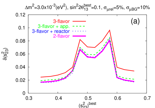
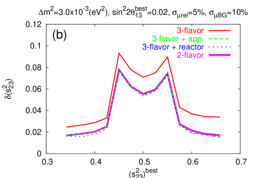
Figure 4: The expected accuracies of $s^{2}_{23}$ determination at 90% CL when combined with $\nu_{e}$ appearance (green dashed line) or reactor measurement of $\theta_{13}$ (blue dotted line). They indicate the improvement over the one reachable by three-flavor analysis of $\nu_{\mu}$ disappearance measurement only, assuming $\sin^{2}{2\theta_{13}}\leq 0.15$, which is indicated by red thin-solid line. The true value of $\sin^{2}{2\theta_{13}}$ is assumed to be 0.1 and 0.02 in Fig. 4a and 4b, respectively. The result of two-flavor analysis (pink thick-solid line), which is given for comparison, is almost degenerate with green dashed and blue dotted lines.

A better sensitivity for $\theta_{23}$ can be achieved by combining some other experiments that are sensitive to $\theta_{13}$ with disappearance measurement, though it cannot solve the problems of the large Jacobian and the degeneracy; An improvement can be expected to the extent that the loss of sensitivity of $\theta_{23}$ is caused by the uncertainty of $\theta_{13}$. There are two possibilities for the supplementary experiments: $\nu_{e}$ appearance measurement in LBL experiments and $\theta_{13}$ measurement in reactor experiments. Fortunately, the $\nu_{\mu}$ disappearance measurement is always accompanied by the simultaneous $\nu_{e}$ appearance measurement of $P(\nu_{\mu}\rightarrow\nu_{e})$ in most of the LBL experiments. Therefore, it is natural to think about combining them first to determine $\theta_{23}$ more precisely. But if a reactor measurement of $\theta_{13}$ is carried out it, it may give a better determination of $\theta_{13}$ than LBL $\nu_{e}$ appearance experiments because the latter suffers from the additional uncertainty due to $\delta$ KMN02 .

Here, we present only the result for $\delta^{\text{best}}=0$. We have checked that when the input value $\delta^{\text{best}}$ is varied in the range $-\pi/2\leq\delta^{\text{best}}\leq\pi/2$ the variation of $\delta(s^{2}_{23})$ is within $\pm 5\%$ relatively to the value for $\delta^{\text{best}}=0$. Note that the $\Delta\chi^{2}$ must be minimized with respect to $\delta$ because we can not know the value of $\delta$ from $\nu_{e}$ appearance only. Again, we postpone the detailed description of our statistical procedure in Appendix C.

The obtained results of how the sensitivity improves with LBL $\nu_{e}$ appearance and reactor measurement are presented in Fig. 4 for two values of $\theta_{13}^{\text{best}}$, $\sin^{2}{2\theta_{13}^{\text{best}}}=0.1$ (Fig. 4a) and 0.02 (Fig. 4b). We examine the cases with two true values of $\sin^{2}{2\theta_{13}}$ because the accuracy of $\sin^{2}{2\theta_{13}}$ measurement in appearance experiments depends on its true value. On the other hand, the error of $\sin^{2}{2\theta_{13}}$ in the reactor-neutrino disappearance measurement is nearly independent of the true value of $\theta_{13}$, $\delta\left(\sin^{2}{2\theta_{13}}\right)\simeq 0.02$ at 90% CL, as was shown in our previous analyses MSYIS ; reactorCP . We utilize this feature to simplify our formulation of the statistical procedure with reactor measurement in Appendix C.

It is shown in Fig. 4 that the accuracy of $\theta_{23}$ measurement is indeed improved thanks to the help by $\nu_{e}$ appearance experiment or reactor measurement of $\theta_{13}$. The reason why the better sensitivity of $\theta_{23}$ is obtained at smaller $\sin^{2}{2\theta_{13}^{\text{best}}}$ in the case with appearance measurement is that the error of $\sin^{2}{2\theta_{13}}$ determination increases for greater values of $\sin^{2}{2\theta_{13}^{\text{best}}}$ due to larger $\sigma_{e{\text{rel}}}^{2}(N^{\text{best}}_{e})^{2}$ in (34). In fact, the case presented in Fig. 4b with $\sin^{2}{2\theta_{13}^{\text{best}}}=0.02$ represents the best sensitivity attainable by combined appearance-disappearance measurement. Notice that the error of $\theta_{23}$ cannot be smaller than that of two-flavor fitting ($\theta_{13}=0$) because it is the limit of no uncertainty in $\theta_{13}$. Moreover, appearance measurement itself is not very sensitive to $\theta_{23}$ and hence it plays only a supplementary role by constraining $\theta_{13}$.

It is also shown in Fig. 4 that with reactor measurement of $\theta_{13}$ the error of $\theta_{23}$ determination is reduced to the one expected in the two-flavor fitting with $\theta_{13}=0$ independent of the values of $\theta_{13}^{\text{best}}$. Thus, the reactor measurement of $\theta_{13}$ can do a better job in improving accuracy of $\theta_{23}$ determination in relatively large $\theta_{13}^{\text{best}}$. It is due to the feature that the uncertainty in $\theta_{13}$ determination in reactor experiments is insensitive to the true values of $\theta_{13}$, and that it is a pure measurement of $\theta_{13}$. In the combined analysis with appearance measurement, by contrast, $\min_{\delta}\Delta\chi_{e}^{2}$ (see Appendix C for definition) vanishes not only at the best fit point but also in region around it due to the minimization in terms of $\delta$, and no improvement of $\Delta\chi_{\mu}^{2}$ is obtained in the region.

We did not attempt to further combine $\nu_{e}$ appearance measurement, because the sensitivity in two-flavor analysis, which can be regarded as the limiting sensitivity attainable by the present method, is already achieved with reactor measurement of $\theta_{13}$.

V Concluding remarks

In the next generation LBL neutrino oscillation experiments, a precise determination of $\sin^{2}{2\theta_{23}}$ to a few % level is expected. In this paper, we have pointed out that, despite such marvelous sensitivities for $\sin^{2}{2\theta_{23}}$, the reachable accuracy of determination of $s^{2}_{23}$ is only at a level of $\delta(s_{23}^{2})/s_{23}^{2}=10\%\mbox{-}20\%$ depending upon the true value of $\theta_{23}$.

We have identified the principal reasons for the disparity between the errors of $\sin^{2}{2\theta_{23}}$ and $s^{2}_{23}$ as due to the Jacobian and the degeneracy effects. We also noticed that measurement of $\theta_{23}$, when it goes down to such high accuracy, is started to be affected by the higher order corrections in $s_{13}^{2}$ in the oscillation probability. We have shown that by doing detailed quantitative analyses such three-flavor effects produce, typically, an increase of uncertainty in $s^{2}_{23}$ determination by $0.008\mbox{-}0.017$; $\delta(s^{2}_{23})$ is larger in the second octant of $\theta_{23}$ than that in the first octant.

Then, we have shown that by combining either reactor measurement of $\theta_{13}$, or $\nu_{e}$ appearance measurement in LBL experiment the accuracies of $\theta_{23}$ determination can be improved to the level expected by simple two-flavor fitting ($\theta_{13}=0$) of the measurement, the limiting sensitivity attainable by the disappearance measurement.

We have to note that our simulation of data and the estimation of uncertainties were done with OA 2 degree beam, which may be slightly higher in peak energy than the one appropriate for $\Delta m^{2}_{31}=2\mbox{-}2.5\times 10^{-3}$eV². It is worthwhile to repeat the analysis with more realistic OA 2.5 degree beam.

Finally, we want to make some remarks on importance of precise determination of the lepton flavor mixing parameters. We want to stress two viewpoints, one related to physics and the other to future neutrino experiments.

(1) Why is precise measurement of the lepton flavor mixing parameters so important?

One of the significant features is that there are two large and small mixing angles. It is suggested that near maximal $\theta_{23}$ may imply a symmetry and $\theta_{23}$ is maximal and $\theta_{13}$ vanishes in the symmetry limit symmetry . If it is indeed the case detecting small deviation of $\theta_{23}$ from the maximal is as important as measuring $\theta_{13}$. Confirmation of this possibility would require a few % level determination of $s^{2}_{23}$, given already severe constraint by the global analysis, $s^{2}_{13}\leq 0.047$ at 3$\sigma$ CL global . If it turned out that $\theta_{13}$ is much smaller, it would necessitate even more accurate determination of $\theta_{23}$. If some of the lepton and quark mixing angles are indeed “complementary” with each other mina-smi , there will be immense requests for precise determination of lepton mixing angles because the quark mixing angles are now measured quite accurately. This possibility may require even more precise determination of $\theta_{23}$ beyond a level expectable by current technology.

Keeping in mind the possibility that we finally uncover the real theory of flavor mixing in the future it is desirable, whenever opportunity exists, to pursue determination of mixing parameters as precisely as possible. Notice that there is a way to measure $\theta_{12}$ to an accuracy of $\simeq$ 2% comparable to that of the Cabibbo angle MNTZ .

(2) How important or crucial is the precise determination of $\theta_{23}$ for future neutrino oscillation experiments?

Most probably the field where precise determination of lepton mixing parameters is really necessary is the detection of leptonic CP violation, one of the ultimate goal of future neutrino experiments. It is because CP violation is a tiny effect, being suppressed by the two small numbers, one the Jarlskog factor $\simeq 0.04\sin{\delta}$ and the other $\epsilon\equiv\Delta m^{2}_{21}/\Delta m^{2}_{31}\simeq 0.033$. Hence, it is crucial to minimize uncertainties of other mixing parameters (as well as neutrino cross sections on the relevant nuclei) to achieve unambiguous detection of CP violation.

In this regard, diminishing the uncertainty in $\theta_{23}$ measurement is probably one of the most important. To obtain the feeling let us suppose for simplicity that the experiment has relatively short baseline so that the vacuum oscillation approximation applies, which may be the case for the JPARC-Hyper-Kamiokande project Hyper-K . Let us assume that the CP asymmetry defined by $A\equiv(P(\nu)-P(\bar{\nu}))/(P(\nu)+P(\bar{\nu}))$ gives a good measure for CP violation, where $P(\nu)$ and $P(\bar{\nu})$ denote appearance probabilities $P(\nu_{\mu}\rightarrow\nu_{e})$ and $P(\bar{\nu}_{\mu}\rightarrow\bar{\nu}_{e})$, respectively. To simplify the equations we tune the energy at the first oscillation maximum, $\Delta m^{2}_{31}L/2E=\pi$, as planned in the J-PARC experiment. Under these approximations, the CP asymmetry is given by

$$A\equiv\frac{P(\nu)-P(\bar{\nu})}{P(\nu)+P(\bar{\nu})}=-\frac{\sin{2\theta_{12}}\cot{\theta_{23}}}{s_{13}}\left(\frac{\Delta m^{2}_{21}L}{4E}\right)\sin\delta.$$ (8)

At the moment, of course, the uncertainty of $s_{13}$ is a dominating error because it has not been measured yet. But it is expected that it can be measured either by LBL or reactor experiments with errors $\simeq 10\mbox{-}25$% if $\sin^{2}{2\theta_{13}}>0.04$. The error produced by $\cot{\theta_{23}}$ factor in (8) is non-negligible compared to this error. The uncertainties estimated in Sec. III can be translated into $\simeq 5\mbox{-}15$% error in $\cot{\theta_{23}}$, and hence it is large. Here, it is worth to note that where the errors are relatively small the splitting of $\cot{\theta_{23}}$ between two degenerate solutions of $\theta_{23}$ is large. Therefore, the uncertainty in the CP asymmetry is even larger, 20-30%, in off the maximal region if the octant degeneracy of $\theta_{23}$ is not resolved. Most likely, the error of $s_{13}$ is significantly reduced at the time of CP measurement because of the possibility that it is precisely determined by in situ LBL measurement employing both neutrino and antineutrino beams at the oscillation maximum (or more precisely the shrunk ellipse limit KMN02 ). Therefore, the uncertainty of $\theta_{23}$ including the degeneracy effect may be the dominating error for CP measurement.

Precise determination of $\Delta m^{2}_{31}$, though not explicitly addressed in this paper, is an another important issue. The error is expected to be $\sim 10$% in the JPARC-SK experiment. Its precise determination is also essential in a variety of contexts ranging search for CP violation and improving bounds on mixing parameters by double beta decay experiments.

In conclusion, we stress the importance of finding alternative methods which are sensitive to $s_{23}$ not to $\sin{2\theta_{23}}$ for accurate measurement of $\theta_{23}$. The obvious candidates include the reactor-LBL combined measurement discussed in MSYIS , and high-statistics observation of atmospheric neutrinos kajita_noon04 ; concha-smi_23 .

Appendix A Derivation of disappearance probability $P(\nu_{\mu}\rightarrow\nu_{\mu})$ to the next to leading order in $\Delta m^{2}_{21}/\Delta m^{2}_{31}$ and $s^{2}_{13}$

In this Appendix, we give a self-contained discussion for deriving the expression of disappearance probability $P(\nu_{\mu}\rightarrow\nu_{\mu})$ which is valid to the next to leading order in $\epsilon$ and $s^{2}_{13}$. We use the method developed by Kimura, Takamura, and Yokomakura (KTY) KTY .

The evolution equation of neutrinos can be written in the flavor eigenstate as

$$i\frac{d}{dx}\nu_{\alpha}=\frac{1}{2E}H_{\alpha\beta}\nu_{\beta}\hskip 42.67912pt(\alpha,\beta=e,\mu,\tau),$$ (9)

where the Hamiltonian is given by

$$H=U\left[\begin{array}[]{ccc}\Delta m^{2}_{11}&0&0\\ 0&\Delta m^{2}_{21}&0\\ 0&0&\Delta m^{2}_{31}\end{array}\right]U^{+}+\left[\begin{array}[]{ccc}a(x)&0&0\\ 0&0&0\\ 0&0&0\end{array}\right],$$ (16)

whose first term will be denoted as $H^{vac}$ hereafter and $\Delta m^{2}_{ji}\equiv m^{2}_{j}-m^{2}_{i}$. (Hence, $\Delta m^{2}_{11}\equiv 0$ by definition.) In (16), $a\equiv 2\sqrt{2}G_{F}N_{e}(x)E$ denotes the index of refraction of neutrinos in medium of electron number density $N_{e}(x)$, where $G_{F}$ is the Fermi constant and $E$ is the neutrino energy wolfenstein . Despite that $N_{e}(x)$ may depend upon locations along the neutrino trajectory, we use constant density approximation throughout this paper. The MNS matrix $U$ relates the flavor and the vacuum mass eigenstates as

$$\nu_{\alpha}=(U)_{\alpha i}\nu_{i},$$ (17)

where $i$ runs over 1-3.

We now define the mass eigenstate in matter $\nu_{i}^{m}$ by using transformation

$$\nu_{\alpha}=(V)_{\alpha i}\nu_{i}^{m},$$ (18)

where $V$ is the unitary matrix which diagonalize the Hamiltonian with scaled eigenvalues $\lambda$ as $V^{\dagger}HV=H_{diag}\equiv diag(a\lambda_{1},a\lambda_{2},a\lambda_{3})$. We first obtain the expressions of the eigenvalues of the Hamiltonian (16). They are determined by the equation $det[H-\lambda aI]=0$ which is the cubic equation for the scaled eigenvalue $\lambda$:

$$\lambda^{3}-(\delta_{21}+\delta_{31}+1)\lambda^{2}+\left[(c_{12}^{2}c_{13}^{2}+s_{13}^{2})\delta_{21}+c_{13}^{2}\delta_{31}+\delta_{21}\delta_{31}\right]\lambda-c_{12}^{2}c_{13}^{2}\delta_{21}\delta_{31}=0.$$ (19)

Notice that everything is scaled by $a$ and $\delta_{21}$ and $\delta_{31}$ denote the scaled squared mass differences,

$$\delta_{21}\equiv\frac{\Delta m^{2}_{21}}{a},\hskip 42.67912pt\delta_{31}\equiv\frac{\Delta m^{2}_{31}}{a}.$$ (20)

To first order in $\delta_{21}$ and $s^{2}_{13}$ the solutions of the equation are given under the convention that $\lambda_{1}<\lambda_{2}<\lambda_{3}$ by

$$\lambda_{1} = c_{12}^{2}\delta_{21},$$

$$\lambda_{2} = 1+s_{12}^{2}\delta_{21}-\frac{\delta_{31}}{\delta_{31}-1}s_{13}^{2},$$

$$\lambda_{3} = \delta_{31}+\frac{\delta_{31}}{\delta_{31}-1}s_{13}^{2}.$$ (21)

Notice that we are in the intermediate energy region between high-energy (atmospheric) and low-energy (solar) level crossings. If we sit on the high-energy region above two level crossings, the expressions for $\lambda_{2}$ and $\lambda_{3}$ must be interchanged. We have checked that the same analytic formulas are obtained, when expressed in terms of observable physical quantities, even if we work in the high-energy region.

We follow the KTY method for deriving $P(\nu_{\mu}\rightarrow\nu_{\mu})$ and write down the equations

$$H_{\mu\mu} = H^{vac}_{\mu\mu},$$

$$H_{ee}H_{\tau\tau}-H_{e\tau}H_{\tau e} = (H^{vac}_{ee}+a)H^{vac}_{\tau\tau}-H^{vac}_{e\tau}H^{vac}_{\tau e}.$$ (22)

They give relationships between mixing matrix in vacuum and in matter as

$$\sum_{i}\lambda_{i}|V_{\mu i}|^{2} = \sum_{i}\frac{\Delta m^{2}_{i1}}{a}|U_{\mu i}|^{2}\equiv p,$$

$$\sum_{ijk}^{cyclic}\lambda_{i}\lambda_{j}|V_{\mu k}|^{2} = \sum_{ijk}^{cyclic}\frac{\Delta m^{2}_{i1}\Delta m^{2}_{j1}}{a^{2}}|U_{\mu k}|^{2}+\sum_{i=1}^{3}\frac{\Delta m^{2}_{i1}}{a}|U_{\tau i}|^{2}\equiv q.$$ (23)

Solving (23) for $|V_{\mu i}|^{2}$ under the constraint of unitarity

$$\sum_{i}|V_{\mu i}|^{2}=1$$ (24)

we obtain

$$|V_{\mu i}|^{2}=\frac{1}{\Delta_{ji}\Delta_{ki}}\left[\lambda_{i}p+q-\lambda_{i}(\lambda_{j}+\lambda_{k})\right],$$ (25)

where $\Delta_{ji}\equiv\lambda_{j}-\lambda_{i}$ and ($i,j,k$) are cyclic.

The disappearance probability $P(\nu_{\mu}\rightarrow\nu_{\mu})$ is given by

$$P(\nu_{\mu}\rightarrow\nu_{\mu})=1-4\sum_{(i,j)}^{cyclic}\frac{L_{ij}}{\Delta_{ij}\Delta_{12}\Delta_{23}\Delta_{31}}\sin^{2}{\left(\frac{\Delta_{ij}aL}{4E}\right)},$$ (26)

where $L_{ij}$ is given by

$$L_{ij} = p^{2}\lambda_{i}\lambda_{j}+q^{2}+pq(\lambda_{i}+\lambda_{j})-p\lambda_{i}\lambda_{j}(\lambda_{i}+\lambda_{j}+2\lambda_{k})$$ (27)

$$-q\Bigl{[}\lambda_{i}(\lambda_{j}+\lambda_{k})+\lambda_{j}(\lambda_{i}+\lambda_{k})\Bigr{]}+\lambda_{i}\lambda_{j}(\lambda_{i}+\lambda_{k})(\lambda_{j}+\lambda_{k}).$$

Notice that $p$ and $q$ are expressed by the vacuum mixing parameters through (23). If we insert the exact form of the eigenvalues $\lambda_{i}$ in (27) we obtain the exact expression of the disappearance probability $P(\nu_{\mu}\rightarrow\nu_{\mu})$, which should be identical with $1-P(\nu_{\mu}\rightarrow\nu_{e})-P(\nu_{\mu}\rightarrow\nu_{\tau})$ computed by KTY KTY .

In this paper, we restrict ourselves into the perturbative expansion and keep terms to order $\delta_{21}$, $s^{2}_{13}$, and $\delta_{21}s_{13}$ for CP $\delta$ sensitive terms. Using the perturbative result of the eigenvalues (21) we obtain, for example,

$$\frac{1}{\Delta_{12}\Delta_{23}\Delta_{31}} = \frac{1}{\delta_{31}(\delta_{31}-1)}\left[1-\frac{\delta_{21}}{\delta_{31}(\delta_{31}-1)}\Bigl{(}\delta_{31}^{2}(s_{12}^{2}-c_{12}^{2})-2\delta_{31}s_{12}^{2}+c_{12}^{2}\Bigr{)}\right.$$ (28)

$$\left.+\frac{s_{13}^{2}}{(\delta_{31}-1)^{2}}\left(\delta_{31}^{2}-4\delta_{31}+1\right)\right].$$

Collecting these formulas, we obtain the expression of the disappearance probability to the next to leading order as

$$1-P(\nu_{\mu}\rightarrow\nu_{\mu})=4(D_{12}+D_{23}+D_{31}),$$ (29)

$$D_{12}+D_{23}=\frac{\delta_{31}^{2}}{(\delta_{31}-1)^{2}}\left[s_{13}^{2}s_{23}^{2}-2\delta_{21}\frac{(\delta_{31}-1)}{\delta_{31}}J^{\prime}_{r}\cos{\delta}\right]$$

$$\times\left[c_{23}^{2}\sin^{2}\left(\frac{aL}{4E}\right)+s_{23}^{2}\sin^{2}\left(\frac{aL}{4E}(\delta_{31}-1)\right)\right],$$ (30)

$$D_{31} = s_{23}^{2}c_{23}^{2}\sin^{2}\left(\frac{aL}{4E}\delta_{31}\right)$$ (31)

$$+ s_{23}^{2}c_{23}^{2}\left[-s_{13}^{2}\frac{\delta_{31}^{2}}{(\delta_{31}-1)^{2}}\sin^{2}\left(\frac{aL}{4E}\delta_{31}\right)+\Bigl{(}-\delta_{21}c_{12}^{2}+\frac{\delta_{31}}{\delta_{31}-1}s_{13}^{2}\Bigr{)}\Bigl{(}\frac{aL}{4E}\Bigr{)}\sin\left(\frac{aL}{2E}\delta_{31}\right)\right]$$

$$+ 2\frac{\delta_{21}}{\delta_{31}(\delta_{31}-1)}\Bigl{(}s_{23}^{2}\delta_{31}^{2}+c_{23}^{2}-s_{23}^{2}\Bigr{)}J^{\prime}_{r}\cos{\delta}\sin^{2}\left(\frac{aL}{4E}\delta_{31}\right),$$

where $J^{\prime}_{r}\equiv c_{12}s_{12}c_{23}s_{23}s_{13}$. The leading order term appears only in $D_{31}$ (the first term). Notice that once we employ perturbation expansion by $\delta_{21}=\Delta m^{2}_{21}/a$ we cannot take the vacuum oscillation limit $a\rightarrow 0$ in (30) and (31).

We also note a pathology in doing perturbative computation of the oscillation probabilities. In energy region around dip at the oscillation maxima, the leading term in the survival probability vanishes and the perturbative expansion is not well defined. In fact, the perturbative formula for $P(\nu_{\mu}\rightarrow\nu_{\mu})$ in (29) becomes slightly negative in the energy region, To obtain better approximation we may have to sum up small terms that are negligible except for this region. In the context of the analysis in this paper, however, we have explicitly checked that the pathological feature does not affect our estimation of the sensitivity.

Appendix B Method for statistical analysis of disappearance experiment

We define our statistical method to quantify our sensitivity analysis for determination of $\theta_{23}$. We use the following standard form of $\Delta\chi^{2}_{\mu}$:

$$\Delta\chi^{2}_{\mu}(s_{23},\Delta m_{31}^{2},s_{13})\equiv\sum_{i}\frac{\left(N_{\mu i}-N_{\mu i}^{\text{best}}\right)^{2}}{N^{\text{best}}_{\mu i}+B_{\mu i}+(\sigma_{\mu{\text{rel}}}N^{\text{best}}_{\mu i})^{2}+(\sigma_{{\mu\text{BG}}}B_{\mu i})^{2}},$$ (32)

where $N_{\mu i}$ denotes the number of $\nu_{\mu}$ charged-current quasi-elastic events of the reaction $\nu_{\mu}+N\rightarrow\mu^{-}+N^{\prime}$ in $i$th energy bin which is to be tested against the artificially created “experimental event number” whose best fit is $N_{\mu i}^{\text{best}}$. $B_{\mu i}$ is the number of background events calculated in the similar way. We use 4 energy bins of width 0.2GeV in the energy range $E_{\nu}=0.4\mbox{-}1.2$GeV. $\sigma_{\mu{\text{rel}}}$ and $\sigma_{{\mu\text{BG}}}$ represent the systematic errors associated with signal and background events, respectively.

To calculate the numbers of signal events we convolute the survival probability $P(\nu_{\mu}\rightarrow\nu_{\mu})$ with the neutrino flux times cross sections given in kameda . We use for $P(\nu_{\mu}\rightarrow\nu_{\mu})$ the expression valid to next to leading order in $\epsilon$ and $s^{2}_{13}$, (29) with (30) and (31). We have explicitly checked that $\delta$-dependent terms gives a minor effect in our analysis because they are of the order of $\epsilon s_{13}$ which are higher order than terms we are keeping (assuming $\epsilon$ and $s^{2}_{13}$ are comparable in size). We assume 5 years running of neutrino mode $\nu_{\mu}$ disappearance measurement. The estimation of background is done by using energy distribution of background events after cut kindly provided by the JPARC-SK group private . We have cross-checked our procedure against the numbers of events after cut.

The procedure of calculating the error of $\theta_{23}$ determination is as follows. We take an input value of $\theta_{13}$ as experimental best fit value (or nature’s choice), and obtain 90% CL allowed region in $s^{2}_{23}\mbox{-}\Delta m^{2}_{31}$, or $\sin^{2}{2\theta_{23}}\mbox{-}\Delta m^{2}_{31}$ plane. To obtain the allowed region, we project three-dimensional manifold of $\Delta\chi^{2}_{\mu}=$ constant onto the above two-dimensional plane by imposing the CHOOZ constraint $s^{2}_{23}<0.04$ ($\sin^{2}{2\theta_{13}}<0.15$) at 90% CL. We rely on the analysis of 2 degrees of freedom because of the resulting two-dimensional plane. Notice that while we take a particular value of $\theta_{13}$ as an input a wide unlimited region is allowed for output value of $\theta_{13}$, as shown in Fig. 1. The feature arises because the disappearance measurement is poor at restricting $\theta_{13}$. Then, $\delta(\sin^{2}{2\theta_{23}})$ and $\delta(s_{23}^{2})$ plotted respectively in Fig. 2 and Fig. 3 are half width of the projected allowed region onto the $\sin^{2}{2\theta_{23}}$ and $s^{2}_{23}$ axis for a value of $\Delta m^{2}_{31}$. We examine cases of two input values of $\theta_{13}$, $\sin^{2}{2\theta_{13}^{\text{best}}}=0.0$ and 0.1 ($(s^{2}_{13})^{\text{best}}=0.026$).

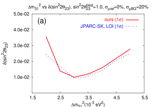
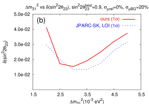
Figure 5: Comparison of our estimate of sensitivity for $\sin^{2}{2\theta_{23}}$ (red solid line) with that of the JPARC-SK group given in LOI (blue dotted line). Both estimates use the two-flavor mixing and the same systematic errors. The input value of $\theta_{23}$ is taken as maximal, $\sin^{2}{2\theta_{23}^{\text{best}}}=1$, in Fig. 5a and as $\sin^{2}{2\theta_{23}^{\text{best}}}=0.9$ in Fig. 5b.

In the JPARC-SK’s LOI JPARC they describe the procedure of determination of $\theta_{23}$ by the $\nu_{\mu}$ disappearance measurement at the neutrino energy that corresponds to the first oscillation maximum. In Fig. 11 of JPARC (original version) they present, based on analysis assuming the two-flavor mixing, the accuracy of determination of $\sin^{2}{2\theta_{23}}$ and $\Delta m^{2}_{31}$ as a function of $\Delta m^{2}_{31}$. To check the consistency of our procedure of computing event numbers as well as the method for statistical analysis we try to reproduce the former figure and the result of this analysis is given in Fig. 5; Fig. 5a and Fig. 5b are for the cases $\sin^{2}{2\theta_{23}^{\text{best}}}=1.0$ and 0.9, respectively, and we have used the two-flavor analysis. We restrict ourselves to the plot of uncertainty of $\sin^{2}{2\theta_{23}}$ because it is of importance for our later analyses. We use $\sigma_{\mu{\text{rel}}}=0\%$ and $\sigma_{{\mu\text{BG}}}=20\%$, and take the earth matter density as $\rho=2.8\,\mbox{g}\cdot\mbox{cm}^{-3}$ as in LOI. Our results reproduce well the error of $\sin^{2}{2\theta_{23}}$ presented in LOI. The agreement is particularly good for $\sin^{2}{2\theta_{23}^{\text{best}}}=1.0$ and is reasonably good for $\sin^{2}{2\theta_{23}^{\text{best}}}=0.9$ in the interesting region of $\Delta m^{2}_{31}$.

Appendix C Combined analysis with the LBL appearance or the reactor experiments

We define $\Delta\chi^{2}$ for the combined analysis with the LBL $\nu_{e}$ appearance experiment as

$$\Delta\chi^{2}_{\mu e}(s_{23},\Delta m^{2}_{31},s_{13}) \equiv \Delta\chi^{2}_{\mu}(s_{23},\Delta m^{2}_{31},s_{13})+\min_{\delta}\Delta\chi^{2}_{e}(s_{13},\delta,s_{23}),$$ (33)

$$\Delta\chi^{2}_{e}(s_{13},\delta,s_{23}) \equiv \frac{\left(N_{e}-N_{e}^{\text{best}}\right)^{2}}{N_{e}^{\text{best}}+B_{e}+\sigma_{e{\text{rel}}}^{2}(N^{\text{best}}_{e})^{2}+\sigma_{e{\text{BG}}}^{2}B_{e}^{2}}.$$ (34)

The numbers of signal and background events are denoted in (34) as $N_{e}$ and $B_{e}$, respectively, which are defined without binning for $\nu_{e}$ appearance. In the analyses in this section, the systematic errors in disappearance and appearance measurement are assumed to be the same, $\sigma_{e{\text{rel}}}=\sigma_{\mu{\text{rel}}}=5\%$ and $\sigma_{e{\text{BG}}}=\sigma_{\mu{\text{BG}}}=10\%$. In the definition of $\Delta\chi^{2}_{e}$, we fix for simplicity $\theta_{23}$ and $\Delta m^{2}_{31}$ at their input values $\theta_{23}^{\text{best}}$ and $(\Delta m^{2}_{31})^{\text{best}}$, respectively. For more details on our treatment of the appearance experiment, see reactorCP . The allowed region is obtained by projecting three-dimensional manifold of $\Delta\chi^{2}_{\mu e}=\mbox{constant}$ onto the $s_{23}^{2}\mbox{-}\Delta m^{2}_{23}$ plane, the similar procedure as we defined in Appendix B for the analysis in Sec. III.

Here are some technical comments on how we simulate the number of events after experimental cut. Reconstruction of neutrino energy can be done for quasi-elastic events but not for inelastic events unless reaction products deposit all the energies and they are detected in the water Cherenkov detector. In our analysis, the relation between reconstructed neutrino energy $E_{\text{rec}}$ of background events and true energy $E_{\nu}$ is assumed to be

$$E_{\text{rec}}=E_{\nu}-0.3{\text{GeV}}$$ (35)

by using the comparison between Monte Carlo simulation done by the JPARC-SK group. See Fig. 2 in JPARC .

For signal events, $E_{\text{rec}}=E_{\nu}$ is assumed. Then, from a spectrum $N_{ac}$ calculated by JPARC-SK group private with a certain set $x_{0}$ of parameter values, the spectrum after cut for any values of parameters $x$ is estimated on a bin-by-bin basis as

$$N_{ac}(x)=\frac{N_{bc}(x)}{N_{bc}(x_{0})}\ N_{ac}(x_{0}),$$ (36)

where $N_{bc}$ represents the calculated number of events before cut. In our analysis, this prescription is used for all number of events in JPARC-SK.

We define $\Delta\chi^{2}$ for the combined analysis with reactor $\theta_{13}$ experiment via the following considerations: The atmospheric $\Delta m_{31}^{2}$ will be determined by the location of the dip in the energy distribution of muons in disappearance measurement corresponding to the first oscillation maximum. Then, the reactor experiments can determine $\theta_{13}$ independent of the other oscillation parameters as well as the matter effect as discussed in MSYIS . Therefore, it acts like giving additional constraint purely on $\theta_{13}$. The appropriate $\Delta\chi^{2}$ then takes a very simple one,

$$\Delta\chi^{2}_{\mu r}(s_{23},\Delta m^{2}_{23},s_{13})\equiv\Delta\chi^{2}_{\mu}(s_{23},\Delta m_{31}^{2},s_{13})+\Delta\chi^{2}_{r}(s_{13}).$$ (37)

For $\Delta\chi^{2}_{r}$ of reactor experiment we use an effective parametrization

$$\Delta\chi^{2}_{r}=\frac{\left(\sin^{2}{2\theta_{13}}-\sin^{2}{2\theta_{13}^{\text{best}}}\right)^{2}}{\sigma_{r}^{2}}$$ (38)

rather than dealing with a particular experimental setup explicitly, where $\sin^{2}{2\theta_{13}^{\text{best}}}$ is the true value of $\sin^{2}{2\theta_{13}}$ assumed in the analysis. Note that the uncertainty in $\sin^{2}{2\theta_{13}}$ in the reactor-neutrino disappearance measurement is almost independent of true value of $\theta_{13}$ as was shown in our previous analyses MSYIS ; reactorCP . This feature is in contrast with the one in the LBL appearance measurement of $\theta_{13}$ mentioned in the previous section. We take, based on the references, $\sigma_{r}=0.02/\sqrt{2.7}$ so that $\delta\left(\sin^{2}{2\theta_{13}}\right)=0.02$ at 90% CL in the analysis with 1 degree of freedom. The effective $\Delta\chi^{2}_{r}$ has a definite merit because it does not depend on details of the particular experiments, and the value of $\sigma_{r}$ is a representative of various different analyses done before.