Fate of oscillating scalar fields in the thermal bath
and their cosmological implications

Abstract

Relaxation process of a coherent scalar field oscillation in the thermal bath is investigated using nonequilibrium quantum field theory. The Langevin-type equation of motion is obtained which has a memory term and both additive and multiplicative noise terms. The dissipation rate of the oscillating scalar field is calculated for various interactions such as Yukawa coupling, three-body scalar interaction, and biquadratic interaction. When the background temperature is larger than the oscillation frequency, the dissipation rate arising from the interactions with fermions is suppressed due to the Pauli blocking, while it is enhanced for interactions with bosons due to the induced effect. In both cases, we find that the microphysical detailed balance relation drives the oscillating field to a thermal equilibrium state. That is, for low-momentum modes, the classical fluctuation-dissipation theorem holds and they relax to a state the equipartition law is satisfied, while higher-momentum modes reach the state the number density of each quanta consists of the thermal boson distribution function and zero-point vacuum contribution. The temperature-dependent dissipation rates obtained here are applied to the late reheating phase of inflationary universe. It is found that in some cases the reheat temperature may take somewhat different value from the conventional estimates, and in an extreme case the inflaton can dissipate its energy without linear interactions that leads to its decay. Furthermore the evaporation rate of the Affleck-Dine field at the onset of its oscillation is calculated.

I Introduction

Cosmology of the early Universe is a useful probe of high energy phenomena beyond the reach of ground based accelerator experiments. The universe at its birth, however, is likely to suffer from huge relic quantum fluctuations and we cannot expect that it started classical evolution from a thermal equilibrium state with a well-defined temperature. Rapid cosmic expansion in the early universe further delays equilibration Ellis:1979nq and it is not likely that the phase transition of grand unified theories occurred thermally Yokoyama:1989pa . Once the energy scale has fallen well below typical grand unification scale, cosmic expansion rate gets smaller than interaction rates of ambient massless particles to establish thermal equilibrium. Phenomenon in such a regime may be studied in terms of quantum field theory at finite temperature neglecting cosmic expansion and using the cosmic temperature at each epoch. If some degrees of freedom are out of equilibrium, then we must of course use nonequilibrium field theories Chou:es . In modern cosmology, we often encounter a situation some scalar fields are in nonequilibrium configuration interacting with thermal background.

Indeed scalar fields play central roles to explain virtually everything we observe—overall homogeneity and isotropy as well as the origin of small density perturbation are attributed to inflation driven by an inflaton scalar field, huge entropy carried by the cosmic microwave (and neutrino) background radiation to the reheating process by the decay of the inflaton Sato:1980yn ; lindebook . Furthermore the observed baryon asymmetry and dark matter may also originate in scalar fields such as squarks and/or sleptons through the Affleck-Dine mechanism Affleck:1984fy and formation of Q-balls Enqvist:2003gh .

Thus it is of utmost importance to clarify the evolution of scalar fields in cosmic medium. In the present paper we study the fate of a coherent scalar field oscillation interacting with fermions or bosons, which are thermally populated, using the nonequilibrium quantum field theory. Such a situation is realized in the late stage of reheating after inflation as well as in the evolution of flat directions in supersymmetric theories which may be associated with Affleck-Dine baryogenesis.

We start with a brief review of a field theoretic method appropriate to analyze time evolution of the expectation value of a scalar field. The standard quantum field theory, which is appropriate for evaluating the transition amplitude from an ‘in’ state to an ‘out’ state for some field operator ${{\cal O}}$, $\left\langle\rm out|\,\mbox{\boldmath${{\cal O}}$}\,|in\right\rangle$, is not suitable to trace time evolution of an expectation value in a non-equilibrium system. In order to follow the time development of the expectation value of some fields, it is necessary to establish an appropriate extension of the quantum field theory, which is often called the in-in formalism. This was first done by Schwinger Sch and developed in Bak ; Kel ; Jordan:ug . This method has been applied to various cosmological problems by a number of authors Mor ; Calzetta:1986ey ; Boyanovsky:vi ; GR ; Boyanovsky:1994me ; Yamaguchi:1996dp ; GM ; Yamaguchi:1997sy ; Yokoyama:1998ju ; Ramsey:1997sa . To name a few, a Langevin equation has been obtained by Morikawa Mor and Gleiser and Ramos GR in the slow-roll limit, which was applied to the electroweak phase transition in Yamaguchi:1996dp and to warm inflation Berera:1995ie in Yokoyama:1998ju . On the other hand, the case of oscillating scalar field was studied by Greiner and Müller who took only the self interaction into account GM . Our work is partially related to it but we consider more general interactions with other fermions and bosons, whose effects are strikingly different from each other as shown in Yamaguchi:1996dp .

We calculate an effective action for a real scalar field $\phi$ perturbatively in the in-in formalism by integrating out fields interacting with $\phi$ assuming that they are in thermal equilibrium distributions at a fixed temperature in a fixed flat spacetime. The resultant effective action is complex-valued as a result of coarse graining of these interacting fields, and it describes dissipation of the system field $\phi$. This complex-valuedness is cured by the introduction of auxiliary fields which act as noise terms, both additive and multiplicative, in the equation of motion. Its derivation from the effective action is reported in the next section.

In §III the equation of motion is explicitly solved in the case only linear terms in $\phi$ are important. We show that each spatial Fourier mode of the scalar field will relax to a value determined by the ratio of the Fourier transform of the noise correlation function and that of the memory kernel in the equation of motion, and it takes the same thermal equilibrium value for all the three interactions discussed there, namely Yukawa coupling, three-body scalar interaction, and biquadratic interaction. This is achieved by the detailed balance relation which also leads to the classical fluctuation-dissipation theorem for low momentum modes. The time scale for the relaxation, which is essentially important for cosmological applications, is also evaluated for respective interactions. The result is quite different depending on the statistical property of the interacting particles.

In §IV the analysis is extended to the multiplicative noises and dissipation. Although we cannot find a solution to the equation of motion in this case, we can still confirm the generalized fluctuation-dissipation relation and obtain the dissipation rate as well.

These formulae are applied to two cosmological situations, namely the late reheating phase after inflation in §V and oscillating flat direction in §VI. Finally §VII is devoted to summary and discussion.

II Effective Action in Nonequilibrium Quantum Field Theory

II.1 Nonequilibrium quantum field theory

We consider the following Lagrangian density of a singlet scalar field $\phi$ interacting with another scalar field $\chi$ and a fermion $\psi$.

$${\cal L}=\frac{1}{2}\,(\partial_{\mu}\phi)^{2}-\frac{1}{2}\,m_{\phi}^{2}\phi^{2}-\frac{1}{4!}\lambda\,\phi^{4}+\frac{1}{2}\,(\partial_{\mu}\chi)^{2}-\frac{1}{2}\,m_{\chi}^{2}\chi^{2}-{\cal M}\phi\chi^{2}-\frac{1}{4}\,h^{2}\chi^{2}\phi^{2}+i\bar{\psi}\gamma^{\mu}\partial_{\mu}\psi-m_{\psi}\bar{\psi}\psi-f\phi\bar{\psi}\psi\>.$$ (1)

When we investigate the time evolution of $\phi$, only the initial condition is fixed, and so the time contour in a generating functional starting from the infinite past must run to the infinite future without fixing the final condition and come back to the infinite past again. The generating functional in the in-in formalism is thus given by

$$Z[J,K,\eta,\bar{\eta}] \equiv \mbox{Tr}\left[T_{p}\left\{\exp\left[i\int_{c}dt\int d^{3}x(J\phi+K\chi+\eta\psi+\bar{\eta}\bar{\psi})\right]\right\}\rho\,\right]$$

$$= \mbox{Tr}\left[T_{-}\left\{\exp\left[i\int_{\infty}^{-\infty}dt\int d^{3}x(J_{-}\phi_{-}+K_{-}\chi_{-}+\eta_{-}\psi_{-}+\bar{\eta}_{-}\bar{\psi}_{-})\right]\right\}\right.$$

$$~{}~{}\left.\times\,T_{+}\left\{\exp\left[i\int_{-\infty}^{\infty}dt\int d^{3}x(J_{+}\phi_{+}+K_{+}\chi_{+}+\eta_{+}\psi_{+}+\bar{\eta}_{+}\bar{\psi}_{+})\right]\right\}\rho\,\right]\>,$$

where the suffix $c$ represents the closed time contour of integration. $X_{+}$ denotes a field component $X$ on the plus-branch ($-\infty$ to $+\infty$) and $X_{-}$ that on the minus-branch ($+\infty$ to $-\infty$). The symbol $T_{p}$ represents the time ordering according to the closed time contour, namely, $T_{+}$ the ordinary time ordering, and $T_{-}$ the anti-time ordering. $J,K,$ and $\eta,~{}\bar{\eta}$ represent the external fields for the scalar and the Dirac fields, respectively. In fact, each external field $J_{+}(K_{+},\eta_{+},\bar{\eta}_{+})$ and $J_{-}(K_{-},\eta_{-},\bar{\eta}_{-})$ is identical, but for technical reasons we treat them differently and set $J_{+}=J_{-}(K_{+}=K_{-},\eta_{+}=\eta_{-},\bar{\eta}_{+}=\bar{\eta}_{-})$ only at the end of calculation. $\rho$ is the initial density matrix. Strictly speaking, we should couple the time development of the expectation value of the field with that of the density matrix, which is practically impossible. Accordingly we assume that deviation from thermal equilibrium is small and use the density matrix corresponding to the finite-temperature state with the exception that the low-momentum modes of $\phi$ may have a larger amplitude initially, whose fate we are interested in. Then the generating functional is described by the path integral as

$$Z[\,J,K,\eta,\bar{\eta}\,] = \exp\biggl{(}\,iW[\,J,K,\eta,\bar{\eta}\,]\,\biggr{)}$$ (3)

$$= \int_{c}{\cal D}\phi\int_{c}{\cal D}\chi\int_{c}{\cal D}\psi\int_{c}{\cal D}\psi^{\ast}\exp{\biggl{(}\,iS[\,\phi,\chi,\psi,\bar{\psi},J,K,\eta,\bar{\eta}\,]\,\biggr{)}}\>,$$

where the classical action $S$ is given by

$$S[\,\phi,\chi,\psi,\bar{\psi},J,K,\eta,\bar{\eta}\,]=\int_{c}d^{4}x\left[{\cal L}+J(x)\phi(x)+K(x)\chi(x)+\eta(x)\psi(x)+\bar{\eta}(x)\bar{\psi}(x)\right]\>.$$ (4)

As with the Euclidean-time formulation, the scalar field is periodic and the Dirac field anti-periodic along the imaginary time direction, with $\phi(t,\mbox{\boldmath${x}$})=\phi(t-i\beta,\mbox{\boldmath${x}$})$, $\chi(t,\mbox{\boldmath${x}$})=\chi(t-i\beta,\mbox{\boldmath${x}$})$, and $\psi(t,\mbox{\boldmath${x}$})=-\psi(t-i\beta,\mbox{\boldmath${x}$})$. Here $\beta$ is the reciprocal of the temperature $T$.

The effective action for the scalar field is defined by the connected generating functional as

$$\Gamma[\phi]=W[\,J,K,\eta,\bar{\eta}\,]-\int_{c}d^{4}xJ(x)\phi(x)\>,$$ (5)

where $\phi(x)=\delta W[J,K,\eta,\bar{\eta}]/\delta J(x)$. In terms of the components along the plus and the minus branches, it reads

$$\Gamma[\phi_{+},\phi_{-}]=W[J_{+},J_{-},\cdots]-\int_{-\infty}^{\infty}dt\int d^{3}x\left[J_{+}(x)\phi_{+}(x)-J_{-}(x)\phi_{-}(x)\right],$$ (6)

with $\phi_{+}(x)=\delta W[J_{+},J_{-},\cdots]/\delta J_{+}(x)$ and $\phi_{-}(x)=-\delta W[J_{+},J_{-},\cdots]/\delta J_{-}(x)$.

We give the finite-temperature propagator before the perturbative expansion. For the closed path, the scalar propagator of $\chi$ has four components consisting of $\chi_{\pm}(x)$ and $\chi_{\pm}(x^{\prime})$.

$$G_{\chi}(x-x^{\prime}) = \left(\begin{array}[]{cc}G^{++}_{\chi}(x-x^{\prime})&G^{+-}_{\chi}(x-x^{\prime})\\ G^{-+}_{\chi}(x-x^{\prime})&G^{--}_{\chi}(x-x^{\prime})\\ \end{array}\right)$$ (9)

$$\equiv \left(\begin{array}[]{cc}\mbox{Tr}[\,T_{+}\chi_{+}(x)\chi_{+}(x^{\prime})\rho\,]&\mbox{Tr}[\,\chi_{-}(x^{\prime})\chi_{+}(x)\rho\,]\\ \mbox{Tr}[\,\chi_{-}(x)\chi_{+}(x^{\prime})\rho\,]&\mbox{Tr}[\,T_{-}\chi_{-}(x)\chi_{-}(x^{\prime})\rho\,]\\ \end{array}\right)$$ (12)

$$= \left(\begin{array}[]{cc}G^{F}_{\chi}(x-x^{\prime})&G^{+}_{\chi}(x-x^{\prime})\\ G^{-}_{\chi}(x-x^{\prime})&G^{\tilde{F}}_{\chi}(x-x^{\prime})\\ \end{array}\right)$$ (15)

$$\equiv \int\frac{d^{4}k}{(2\pi)^{4}}e^{-ik(x-x^{\prime})}\left(\begin{array}[]{cc}G^{F}_{\chi}(k)&G^{+}_{\chi}(k)\\ G^{-}_{\chi}(k)&G^{\tilde{F}}_{\chi}(k)\\ \end{array}\right)\>,$$ (18)

where

$$G^{F}_{\chi}(k) = \frac{i}{k^{2}-m_{\chi}^{2}+i\epsilon}+2\pi n_{B}(\omega_{k})\,\delta(k^{2}-m_{\chi}^{2})\>,$$

$$G^{\tilde{F}}_{\chi}(k) = \frac{-i}{k^{2}-m_{\chi}^{2}-i\epsilon}+2\pi n_{B}(\omega_{k})\,\delta(k^{2}-m_{\chi}^{2})\>,$$

$$G^{+}_{\chi}(k) = 2\pi\,[\,\theta(-k_{0})+n_{B}(\omega_{k})\,]\,\delta(k^{2}-m_{\chi}^{2})\>,$$

$$G^{-}_{\chi}(k) = 2\pi\,[\,\theta(k_{0})+n_{B}(\omega_{k})\,]\,\delta(k^{2}-m_{\chi}^{2})\>,$$ (19)

with $n_{B}(\omega_{k})=(e^{\beta\omega_{k}}-1)^{-1}$,  $\omega_{k}=\sqrt{\mbox{\boldmath${k}$}^{2}+m_{\chi}^{2}}$,  and $\epsilon(k_{0})=\theta(k_{0})-\theta(-k_{0})$ pro . Similar formulae apply for $\phi$ field as well.

The propagator for a Dirac fermion is given by

$$S_{\psi}(x-x^{\prime}) = \left(\begin{array}[]{cc}S^{++}_{\psi}(x-x^{\prime})&S^{+-}_{\psi}(x-x^{\prime})\\ S^{-+}_{\psi}(x-x^{\prime})&S^{--}_{\psi}(x-x^{\prime})\\ \end{array}\right)$$ (22)

$$\equiv \left(\begin{array}[]{cc}\mbox{Tr}[\,T_{+}\psi_{+}(x)\bar{\psi}_{+}(x^{\prime})\rho\,]&\mbox{Tr}[\,-\bar{\psi}_{-}(x^{\prime})\psi_{+}(x)\rho\,]\\ \mbox{Tr}[\,\psi_{-}(x)\bar{\psi}_{+}(x^{\prime})\rho\,]&\mbox{Tr}[\,T_{-}\psi_{-}(x)\bar{\psi}_{-}(x^{\prime})\rho\,]\\ \end{array}\right)$$ (25)

$$\equiv \left(\begin{array}[]{cc}S^{F}_{\psi}(x-x^{\prime})&S^{+}_{\psi}(x-x^{\prime})\\ S^{-}_{\psi}(x-x^{\prime})&S^{\tilde{F}}_{\psi}(x-x^{\prime})\\ \end{array}\right)$$ (28)

$$\equiv \int\frac{d^{4}k}{(2\pi)^{4}}e^{-ik(x-x^{\prime})}\left(\begin{array}[]{cc}S^{F}_{\psi}(k)&S^{+}_{\psi}(k)\\ S^{-}_{\psi}(k)&S^{\tilde{F}}_{\psi}(k)\\ \end{array}\right)\>,$$ (31)

where

$$S^{F}_{\psi}(k) = \frac{i}{\not{k}-m_{\psi}+i\epsilon}-2\pi n_{F}(E_{k})(\not{k}+m_{\psi})\,\delta(k^{2}-m_{\psi}^{2})\>,$$

$$S^{\tilde{F}}_{\psi}(k) = \frac{-i}{\not{k}-m_{\psi}-i\epsilon}-2\pi n_{F}(E_{k})(\not{k}+m_{\psi})\,\delta(k^{2}-m_{\psi}^{2})\>,$$

$$S^{+}_{\psi}(k) = 2\pi\,[\,\theta(-k_{0})-n_{F}(E_{k})\,]\,(\not{k}+m_{\psi})\,\delta(k^{2}-m_{\psi}^{2})\>,$$

$$S^{-}_{\psi}(k) = 2\pi\,[\,\theta(k_{0})-n_{F}(E_{k})\,]\,(\not{k}+m_{\psi})\,\delta(k^{2}-m_{\psi}^{2})\>,$$ (32)

with $n_{F}(E_{k})=(e^{\beta E_{k}}+1)^{-1},\,E_{k}\equiv\sqrt{\mbox{\boldmath${k}$}^{2}+m_{\psi}^{2}}$ pro .

II.2 Perturbative expansion of the finite-temperature effective action

The perturbative loop expansion for the effective action $\Gamma$ can be obtained by transforming $\phi\rightarrow\phi_{cl}+\zeta$ where $\phi_{cl}$ is the field configuration which extremizes the classical action $S[\,\phi,J\,]$ and $\zeta$ is small perturbation around $\phi_{cl}$. Up to two loop order and ${\cal O}(\lambda^{2},h^{4},f^{2})$, $\Gamma$ is made up of the graphs as those depicted in Fig. 1 etc. Summing up these graphs, the effective action $\Gamma$ becomes

$$\Gamma[\phi_{+},\phi_{-}] = \int d^{4}x\left[\frac{1}{2}(\partial\phi_{+})^{2}-\frac{1}{2}(\partial\phi_{-})^{2}-\frac{1}{2}m_{\phi}^{2}\left(\phi_{+}^{2}(x)-\phi_{-}^{2}(x)\right)-\frac{\lambda}{4!}\left(\phi_{+}^{4}(x)-\phi_{-}^{4}(x)\right)\right]$$ (33)

$$+\sum_{j=1}^{8}L_{j}[\phi_{+},\phi_{-}]+\cdots,$$

where each of $L_{j}[\phi_{+},\phi_{-}]$ corresponds to each graph in Fig. 1 and is given as follows.

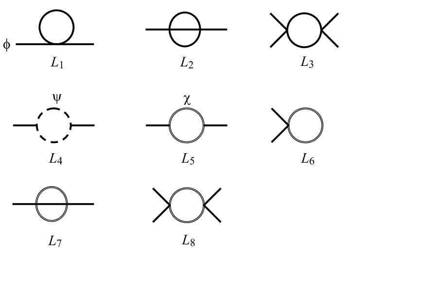
Figure 1: Feynman diagrams corresponding to each term of the effective action. Solid line denotes $\phi$, while broken line and double line represent $\psi$ and $\chi$, respectively.

$$L_{1} = -\frac{\lambda}{4}\int d^{4}xG_{\phi}^{++}(0)\left[\phi_{+}^{2}(x)-\phi_{-}^{2}(x)\right],$$ (34)

$$L_{2} = \frac{i\lambda^{2}}{12}\int d^{4}xd^{4}x^{\prime}\left[\phi_{+}(x)G_{\phi}^{++}(x-x^{\prime})^{3}\phi_{+}(x^{\prime})-\phi_{-}(x)G_{\phi}^{-+}(x-x^{\prime})^{3}\phi_{+}(x^{\prime})\right.$$ (35)

$$\qquad\left.-\phi_{+}(x)G_{\phi}^{+-}(x-x^{\prime})^{3}\phi_{-}(x^{\prime})+\phi_{-}(x)G_{\phi}^{--}(x-x^{\prime})^{3}\phi_{-}(x^{\prime})\right],$$

$$L_{3} = \frac{i\lambda^{2}}{16}\int d^{4}xd^{4}x^{\prime}\left[\phi_{+}^{2}(x)G_{\phi}^{++}(x-x^{\prime})^{2}\phi_{+}^{2}(x^{\prime})-\phi_{-}^{2}(x)G_{\phi}^{-+}(x-x^{\prime})^{2}\phi_{+}^{2}(x^{\prime})\right.$$ (36)

$$\qquad\left.-\phi_{+}^{2}(x)G_{\phi}^{+-}(x-x^{\prime})^{2}\phi_{-}^{2}(x^{\prime})+\phi_{-}^{2}(x)G_{\phi}^{--}(x-x^{\prime})^{2}\phi_{-}^{2}(x^{\prime})\right],$$

$$L_{4} = -\frac{if^{2}}{2}\int d^{4}xd^{4}x^{\prime}\left[\phi_{+}(x)S^{++}_{\psi}(x-x^{\prime})S^{++}_{\psi}(x^{\prime}-x)\phi_{+}(x^{\prime})\right.$$ (37)

$$\qquad\left.-\phi_{-}(x)S^{-+}_{\psi}(x-x^{\prime})S^{+-}_{\psi}(x^{\prime}-x)\phi_{+}(x^{\prime})-\phi_{+}(x)S^{+-}_{\psi}(x-x^{\prime})S^{-+}_{\psi}(x^{\prime}-x)\phi_{-}(x^{\prime})\right.$$

$$\qquad\left.+\phi_{-}(x)S^{--}_{\psi}(x-x^{\prime})S^{--}_{\psi}(x^{\prime}-x)\phi_{-}(x^{\prime})\right],$$

$$L_{5} = i{\cal M}^{2}\int d^{4}xd^{4}x^{\prime}\left[\phi_{+}(x)G_{\chi}^{++}(x-x^{\prime})^{2}\phi_{+}(x^{\prime})-\phi_{-}(x)G_{\chi}^{-+}(x-x^{\prime})^{2}\phi_{+}(x^{\prime})\right.$$ (38)

$$\qquad\left.-\phi_{+}(x)G_{\chi}^{+-}(x-x^{\prime})^{2}\phi_{-}(x^{\prime})+\phi_{-}(x)G_{\chi}^{--}(x-x^{\prime})^{2}\phi_{-}(x^{\prime})\right],$$

$$L_{6} = -\frac{h^{2}}{4}\int d^{4}xG_{\chi}^{++}(0)\left[\phi_{+}^{2}(x)-\phi_{-}^{2}(x)\right],$$ (39)

$$L_{7} = \frac{ih^{4}}{4}\int d^{4}xd^{4}x^{\prime}\left[\phi_{+}(x)G_{\phi}^{++}(x-x^{\prime})G_{\chi}^{++}(x-x^{\prime})^{2}\phi_{+}(x^{\prime})\right.$$ (40)

$$\qquad-\phi_{-}(x)G_{\phi}^{-+}(x-x^{\prime})G_{\chi}^{-+}(x-x^{\prime})^{2}\phi_{+}(x^{\prime})$$

$$\qquad-\phi_{+}(x)G_{\phi}^{+-}(x-x^{\prime})G_{\chi}^{+-}(x-x^{\prime})^{2}\phi_{-}(x^{\prime})$$

$$\qquad\left.+\phi_{-}(x)G_{\phi}^{--}(x-x^{\prime})G_{\chi}^{--}(x-x^{\prime})^{2}\phi_{-}(x^{\prime})\right],$$

$$L_{8} = \frac{ih^{4}}{16}\int d^{4}xd^{4}x^{\prime}\left[\phi_{+}^{2}(x)G_{\chi}^{++}(x-x^{\prime})^{2}\phi_{+}^{2}(x^{\prime})-\phi_{-}^{2}(x)G_{\chi}^{-+}(x-x^{\prime})^{2}\phi_{+}^{2}(x^{\prime})\right.$$ (41)

$$\qquad\left.-\phi_{+}^{2}(x)G_{\chi}^{+-}(x-x^{\prime})^{2}\phi_{-}^{2}(x^{\prime})+\phi_{-}^{2}(x)G_{\chi}^{--}(x-x^{\prime})^{2}\phi_{-}^{2}(x^{\prime})\right].$$

It is convenient to introduce new variables

$$\phi_{c}\equiv\frac{1}{2}(\phi_{+}+\phi_{-})~{}~{}{\rm and}~{}~{}\phi_{\Delta}\equiv\phi_{+}-\phi_{-}$$ (42)

to rewrite the effective action in terms of these variables. As will be seen in (71), $\phi_{\Delta}$ is a response field and $\phi_{c}$ is the physical field. We find

$$\Gamma[\phi_{c},\phi_{\Delta}] = \int d^{4}x\left[-\phi_{\Delta}(x)\Box\phi_{c}(x)-m_{\phi}^{2}\phi_{\Delta}(x)\phi_{c}(x)-\frac{\lambda}{4!}\left(\phi_{\Delta}^{3}(x)\phi_{c}(x)+4\phi_{\Delta}(x)\phi_{c}^{3}(x)\right)\right]$$ (43)

$$+\sum_{j=1}^{8}L_{j}[\phi_{c},\phi_{\Delta}]+\cdots,$$

with

$$L_{1} = -\frac{\lambda}{2}\int d^{4}xG_{\phi}^{++}(0)\phi_{\Delta}(x)\phi_{c}(x),$$ (44)

$$L_{2} = -\frac{\lambda^{2}}{3}\int d^{4}xd^{4}x^{\prime}\mbox{Im}\left[G_{\phi}^{++}(x-x^{\prime})^{3}\right]\phi_{\Delta}(x)\phi_{c}(x^{\prime})\theta(t_{1}-t_{2})$$ (45)

$$+\frac{i\lambda^{2}}{12}\int d^{4}xd^{4}x^{\prime}\mbox{Re}\left[G_{\phi}^{++}(x-x^{\prime})^{3}\right]\phi_{\Delta}(x)\phi_{\Delta}(x^{\prime}),$$

$$L_{3} = -\frac{\lambda^{2}}{2}\int d^{4}xd^{4}x^{\prime}\mbox{Im}\left[G_{\phi}^{++}(x-x^{\prime})^{2}\right]\left(\phi_{\Delta}(x)\phi_{c}(x)\phi_{c}^{2}(x^{\prime})+\textstyle{\frac{1}{4}}\phi_{\Delta}(x)\phi_{\Delta}^{2}(x^{\prime})\phi_{c}(x)\right)\theta(t_{1}-t_{2})$$ (46)

$$+\frac{i\lambda^{2}}{4}\int d^{4}xd^{4}x^{\prime}\mbox{Re}\left[G_{\phi}^{++}(x-x^{\prime})^{2}\right]\phi_{\Delta}(x)\phi_{\Delta}(x^{\prime})\phi_{c}(x)\phi_{c}(x^{\prime}),$$

$$L_{4} = 2f^{2}\int d^{4}xd^{4}x^{\prime}\mbox{Im}\left[S^{++}_{\psi}(x-x^{\prime})S^{++}_{\psi}(x^{\prime}-x)\right]\phi_{\Delta}(x)\phi_{c}(x^{\prime})\theta(t_{1}-t_{2})$$ (47)

$$-\frac{if^{2}}{2}\int d^{4}xd^{4}x^{\prime}\mbox{Re}\left[S^{++}_{\psi}(x-x^{\prime})S^{++}_{\psi}(x^{\prime}-x)\right]\phi_{\Delta}(x)\phi_{\Delta}(x^{\prime}),$$

$$L_{5} = -4{\cal M}^{2}\int d^{4}xd^{4}x^{\prime}\mbox{Im}\left[G_{\chi}^{++}(x-x^{\prime})^{2}\right]\phi_{\Delta}(x)\phi_{c}(x^{\prime})\theta(t_{1}-t_{2})$$ (48)

$$+i{\cal M}\int d^{4}xd^{4}x^{\prime}\mbox{Re}\left[G_{\chi}^{++}(x-x^{\prime})^{2}\right]\phi_{\Delta}(x)\phi_{\Delta}(x^{\prime}),$$

$$L_{6} = -\frac{h^{2}}{2}\int d^{4}xG_{\chi}^{++}(0)\phi_{\Delta}(x)\phi_{c}(x),$$ (49)

$$L_{7} = -h^{4}\int d^{4}xd^{4}x^{\prime}\mbox{Im}\left[G_{\phi}^{++}(x-x^{\prime})G_{\chi}^{++}(x-x^{\prime})^{2}\right]\phi_{\Delta}(x)\phi_{c}(x^{\prime})\theta(t_{1}-t_{2})$$ (50)

$$+\frac{ih^{4}}{4}\int d^{4}xd^{4}x^{\prime}\mbox{Re}\left[G_{\phi}^{++}(x-x^{\prime})G_{\chi}^{++}(x-x^{\prime})^{2}\right]\phi_{\Delta}(x)\phi_{\Delta}(x^{\prime}),$$

$$L_{8} = -\frac{h^{4}}{2}\int d^{4}xd^{4}x^{\prime}\mbox{Im}\left[G_{\chi}^{++}(x-x^{\prime})^{2}\right]\left[\phi_{\Delta}(x)\phi_{c}(x)\phi_{c}^{2}(x^{\prime})+\textstyle{\frac{1}{4}}\phi_{\Delta}(x)\phi_{\Delta}^{2}(x^{\prime})\phi_{c}(x)\right]\theta(t_{1}-t_{2})$$ (51)

$$+\frac{ih^{4}}{4}\int d^{4}xd^{4}x^{\prime}\mbox{Re}\left[G_{\chi}^{++}(x-x^{\prime})^{2}\right]\phi_{\Delta}(x)\phi_{\Delta}(x^{\prime})\phi_{c}(x)\phi_{c}(x^{\prime}).$$

Among these terms, $L_{1}$ and $L_{6}$ are corrections to the mass term of $\phi$, while other terms have both real and imaginary parts. As a result we find

$$\Gamma[\phi_{c},\phi_{\Delta}]=\int d^{4}x\left\{-\phi_{\Delta}(x)[\,\Box+M^{2}\,]\phi_{c}(x)-\frac{\lambda}{4!}\left[4\phi_{\Delta}(x)\phi_{c}^{3}(x)+\phi_{c}(x)\phi_{\Delta}^{3}(x)\right]\right\}$$

$$-\int d^{4}xd^{4}x^{\prime}\left[\,A_{2}(x-x^{\prime})+A_{4}(x-x^{\prime})+A_{5}(x-x^{\prime})+A_{7}(x-x^{\prime})\,\right]\theta(t_{1}-t_{2})\phi_{\Delta}(x)\phi_{c}(x^{\prime})$$

$$-\int d^{4}xd^{4}x^{\prime}\left[\,A_{3}(x-x^{\prime})+A_{8}(x-x^{\prime})\,\right]\theta(t_{1}-t_{2})$$

$$\qquad\qquad\qquad\times\left[\phi_{\Delta}(x)\phi_{c}(x)\phi_{c}^{2}(x^{\prime})+\textstyle{\frac{1}{4}}\phi_{\Delta}(x)\phi_{\Delta}^{2}(x^{\prime})\phi_{c}(x)\right]$$

$$+\frac{i}{2}\int d^{4}xd^{4}x^{\prime}\left\{\,\left[B_{2}(x-x^{\prime})+B_{4}(x-x^{\prime})+B_{5}(x-x^{\prime})+B_{7}(x-x^{\prime})\right]\phi_{\Delta}(x)\phi_{\Delta}(x^{\prime})\right.$$

$$\left.\qquad\qquad\qquad+\left[\,B_{3}(x-x^{\prime})+B_{8}(x-x^{\prime})\,\right]\phi_{\Delta}(x)\phi_{\Delta}(x^{\prime})\phi_{c}(x)\phi_{c}(x^{\prime})\,\,\right\}\>,$$ (52)

where

$$M^{2}=m_{\phi}^{2}+\lambda N(m_{\phi})+2h^{2}N(m_{\chi}),~{}~{}~{}N(m_{i})\equiv\int\!\frac{d^{3}q}{(2\pi)^{3}}\frac{1+2n_{B}(\omega_{q})}{4\omega_{q}},~{}\omega_{q}\equiv\sqrt{{\mbox{\boldmath${q}$}}^{2}+m_{i}^{2}},$$ (53)

$$A_{2}(x-x^{\prime}) = \frac{\lambda^{2}}{3}\mbox{Im}\left[G_{\phi}^{F}(x-x^{\prime})^{3}\right]\>,$$ (54)

$$A_{3}(x-x^{\prime}) = \frac{\lambda^{2}}{2}\mbox{Im}\left[G_{\phi}^{F}(x-x^{\prime})^{2}\right]\>,$$ (55)

$$A_{4}(x-x^{\prime}) = -2f^{2}\mbox{Im}\left\{\mbox{tr}\left[S^{F}_{\psi}(x-x^{\prime})S^{F}_{\psi}(x^{\prime}-x)\right]\right\}\>,$$ (56)

$$A_{5}(x-x^{\prime}) = 4{\cal M}^{2}\mbox{Im}\left[G_{\chi}^{F}(x-x^{\prime})^{2}\right]\>,$$ (57)

$$A_{7}(x-x^{\prime}) = h^{4}\mbox{Im}\left[G_{\phi}^{F}(x-x^{\prime})G_{\chi}^{F}(x-x^{\prime})^{2}\right]\>,$$ (58)

$$A_{8}(x-x^{\prime}) = \frac{h^{4}}{2}\mbox{Im}\left[G_{\chi}^{F}(x-x^{\prime})^{2}\right]\>,$$ (59)

$$B_{2}(x-x^{\prime}) = \frac{\lambda^{2}}{6}\mbox{Re}\left[G_{\phi}^{F}(x-x^{\prime})^{3}\right]\>,$$ (60)

$$B_{3}(x-x^{\prime}) = \frac{\lambda^{2}}{2}\mbox{Re}\left[G_{\phi}^{F}(x-x^{\prime})^{2}\right]\>,$$ (61)

$$B_{4}(x-x^{\prime}) = -f^{2}\mbox{Re}\left\{\mbox{tr}\left[S^{F}_{\psi}(x-x^{\prime})S^{F}_{\psi}(x^{\prime}-x)\right]\right\}\>,$$ (62)

$$B_{5}(x-x^{\prime}) = 2{\cal M}^{2}\mbox{Re}\left[G_{\chi}^{F}(x-x^{\prime})^{2}\right]\>,$$ (63)

$$B_{7}(x-x^{\prime}) = \frac{h^{4}}{2}\mbox{Re}\left[G_{\phi}^{F}(x-x^{\prime})G_{\chi}^{F}(x-x^{\prime})^{2}\right]\>,$$ (64)

$$B_{8}(x-x^{\prime}) = \frac{h^{4}}{2}\mbox{Re}\left[G_{\chi}^{F}(x-x^{\prime})^{2}\right]\>.$$ (65)

Apparently, $A_{j}$ and $B_{j}$ are related with the real and the imaginary parts of $L_{j}$, respectively. The above expressions for $A_{j}(x-x^{\prime})$ are valid only for $t_{1}-t_{2}>0$. We find

$$A_{j}(\mbox{\boldmath${x}$}^{\prime}-\mbox{\boldmath${x}$},t_{1}-t_{2}) = A_{j}(\mbox{\boldmath${x}$}-\mbox{\boldmath${x}$}^{\prime},t_{1}-t_{2}),$$ (66)

$$A_{j}(\mbox{\boldmath${x}$}-\mbox{\boldmath${x}$}^{\prime},t_{2}-t_{1}) = -A_{j}(\mbox{\boldmath${x}$}-\mbox{\boldmath${x}$}^{\prime},t_{1}-t_{2}),$$ (67)

for $t_{2}-t_{1}<0$, although only those with $t_{1}-t_{2}>0$ appear in the final expressions. We also find

$$B_{j}(\mbox{\boldmath${x}$}^{\prime}-\mbox{\boldmath${x}$},t_{1}-t_{2}) = B_{j}(\mbox{\boldmath${x}$}-\mbox{\boldmath${x}$}^{\prime},t_{1}-t_{2}),$$ (68)

$$B_{j}(\mbox{\boldmath${x}$}-\mbox{\boldmath${x}$}^{\prime},t_{2}-t_{1}) = B_{j}(\mbox{\boldmath${x}$}-\mbox{\boldmath${x}$}^{\prime},t_{1}-t_{2}).$$ (69)

The imaginary parts of the effective action represent dissipative effects and we can obtain real effective action by introducing auxiliary random Gaussian fields, $\xi_{a}(x)$ and $\xi_{m}(x)$, as follows.

$$\exp(i\Gamma[\phi_{c},\phi_{\Delta}])=\int{\cal D}\xi_{a}\int{\cal D}\xi_{m}P_{a}[\xi_{a}]P_{m}[\xi_{m}]\exp\left\{i\Gamma_{\rm eff}[\,\phi_{c},\phi_{\Delta},\xi_{a},\xi_{m}\,]\right\}\>,$$ (70)

where

$$\Gamma_{\rm eff}[\,\phi_{c},\phi_{\Delta},\xi_{a},\xi_{m}\,]\equiv\mbox{Re}\Gamma[\phi_{c},\phi_{\Delta}]+\int d^{4}x[\,\xi_{a}(x)\phi_{\Delta}(x)+\xi_{m}(x)\phi_{c}(x)\phi_{\Delta}(x)\,]\>.$$ (71)

Here $P_{a}[\xi_{a}]$ and $P_{m}[\xi_{m}]$ are the probability distribution functionals defined by

$$P_{a}[\xi_{a}]~{}~{}~{} \equiv {\cal N}_{a}\exp\left[\,-\frac{1}{2}\int d^{4}xd^{4}x^{\prime}\xi_{a}(x)D_{a}^{-1}(x-x^{\prime})\xi_{a}(x^{\prime})\,\right],$$ (72)

$$D_{a}(x-x^{\prime}) \equiv B_{2}(x-x^{\prime})+B_{4}(x-x^{\prime})+B_{5}(x-x^{\prime})+B_{7}(x-x^{\prime})\>.$$ (73)

$$P_{m}[\xi_{m}]~{}~{}~{} \equiv {\cal N}_{m}\exp\left[\,-\frac{1}{2}\int d^{4}xd^{4}x^{\prime}\xi_{m}(x)D_{m}^{-1}(x-x^{\prime})\xi_{m}(x^{\prime})\,\right],$$ (74)

$$D_{m}(x-x^{\prime}) \equiv B_{3}(x-x^{\prime})+B_{8}(x-x^{\prime}),\>.$$ (75)

respectively. Thus the dispersions of $\xi_{a}(x)$ and $\xi_{m}(x)$ are given by $B_{j}$. In the above expressions ${\cal N}_{a}$ and ${\cal N}_{m}$ are normalization factors, while the inverse $D^{-1}_{i}(x-y)$ is defined by the relation

$$\int d^{4}yD^{-1}_{i}(x-y)D_{i}(y-z)=\delta(x-z).$$ (76)

II.3 Equation of motion

Applying the variational principle to $\Gamma_{\rm eff}$, we obtain the equation of motion for $\phi_{c}$ containing no imaginary quantity.

$$\left.\frac{\delta\Gamma_{\rm eff}[\,\phi_{c},\phi_{\Delta},\xi_{a},\xi_{m}\,]}{\delta\phi_{\Delta}}\biggl{.}\right|_{\phi_{\Delta}=0}=0\>.$$ (77)

From (71), it reads

$$(\,\Box+M^{2}\,)\,\phi_{c}(x)+\frac{\lambda}{3!}\phi_{c}^{3}(x)+\int_{-\infty}^{t}dt^{\prime}\int d^{3}x^{\prime}C_{a}(x-x^{\prime})\phi_{c}(x^{\prime})$$

$$\qquad\qquad\qquad+\phi_{c}(x)\int_{-\infty}^{t}dt^{\prime}\int d^{3}x^{\prime}C_{m}(x-x^{\prime})\phi_{c}^{2}(x^{\prime})=\xi_{a}(x)+\phi_{c}(x)\xi_{m}(x)\>,$$ (78)

with

$$C_{a}(x-x^{\prime}) \equiv A_{2}(x-x^{\prime})+A_{4}(x-x^{\prime})+A_{5}(x-x^{\prime})+A_{7}(x-x^{\prime}),$$ (79)

$$C_{m}(x-x^{\prime}) \equiv A_{3}(x-x^{\prime})+A_{8}(x-x^{\prime}).$$ (80)

We shall call these two functions memory kernels because the last two terms in the left-hand-side of (78) are nonlocal in time. They will reduce to the dissipation terms and perturbative corrections to the classical equation of motion which would become a part of the derivative of the effective potential, $V^{\prime}_{\rm eff}(\phi)$, if we restricted $\phi(x^{\prime})$ to be a constant in space and time. In this equation of motion $\xi_{a}(x)$ should be regarded as an additive random Gaussian noise with the dispersion,

$$\left\langle\,\xi_{a}(x)\xi_{a}(x^{\prime})\,\right\rangle=D_{a}(x-x^{\prime})\>,$$ (81)

and $\xi_{m}(x)$ is a multiplicative random Gaussian noise acting on $\phi_{c}(x)$ with the dispersion,

$$\left\langle\,\xi_{m}(x)\xi_{m}(x^{\prime})\,\right\rangle=D_{m}(x-x^{\prime})\>.$$ (82)

III Analysis in the linear regime

III.1 Equation of motion in the Fourier space

Here we concentrate on the case only linear terms of $\phi_{c}$ are important and multiplicative noise is negligible in the equation of motion (78). Then the equation of motion reads

$$(\,\Box+M^{2}\,)\,\phi_{c}(x)+\int_{-\infty}^{t}dt^{\prime}\int d^{3}x^{\prime}C_{a}(x-x^{\prime})\phi_{c}(x^{\prime})=\xi_{a}(x)\>.$$ (83)

Hereafter we omit the suffix $c$.

In this regime it is convenient to rewrite the above equation in the wavenumber space. Defining the spatial Fourier transform as

$$\phi_{\mbox{\boldmath\tiny${k}$}}(t) \equiv \int d^{3}x\phi(\mbox{\boldmath${x}$},t)e^{-i\mbox{\boldmath\tiny${k}$}\cdot\mbox{\boldmath\tiny${x}$}},~{}~{}~{}\xi_{\mbox{\boldmath\tiny${k}$}}(t)\equiv\int d^{3}x\xi_{a}(\mbox{\boldmath${x}$},t)e^{-i\mbox{\boldmath\tiny${k}$}\cdot\mbox{\boldmath\tiny${x}$}},$$ (84)

$$C_{a\mbox{\boldmath\tiny${k}$}}(t-t^{\prime}) \equiv \int d^{3}xC_{a}(\mbox{\boldmath${x}$},t-t^{\prime})e^{-i\mbox{\boldmath\tiny${k}$}\cdot\mbox{\boldmath\tiny${x}$}},$$ (85)

we find

$$\ddot{\phi}_{\mbox{\boldmath\tiny${k}$}}(t)+\left(\mbox{\boldmath${k}$}^{2}+M^{2}\right)\phi_{\mbox{\boldmath\tiny${k}$}}(t)+\int_{-\infty}^{t}dt^{\prime}C_{a\mbox{\boldmath\tiny${k}$}}(t-t^{\prime})\phi_{\mbox{\boldmath\tiny$k$}}(t^{\prime})=\xi_{\mbox{\boldmath\tiny${k}$}}(t)\>,$$ (86)

where $C_{a\mbox{\boldmath\tiny${k}$}}(t-t^{\prime})$ is a real function thanks to (66). Here the noise term in the Fourier space, $\xi_{\mbox{\boldmath\tiny${k}$}}(t)$, is a random Gaussian variable with the dispersion,

$$\langle\xi_{\mbox{\boldmath\tiny${k}$}}(t)\xi^{\ast}_{\mbox{\boldmath\tiny${k}$}^{\prime}}(t^{\prime})\rangle=\int d^{3}xD_{a}(\mbox{\boldmath${x}$},t-t^{\prime})e^{-i\mbox{\boldmath\tiny${k}$}\cdot\mbox{\boldmath\tiny${x}$}}(2\pi)^{3}\delta(\mbox{\boldmath${k}$}-\mbox{\boldmath${k}$}^{\prime})\equiv D_{a\mbox{\boldmath\tiny${k}$}}(t-t^{\prime})(2\pi)^{3}\delta(\mbox{\boldmath${k}$}-\mbox{\boldmath${k}$}^{\prime}).$$ (87)

Thus each Fourier mode is completely decoupled from each other in the linear regime even in the presence of the noise term, as it should be.

Equation (86) can be solved in terms of the Fourier transform with respect to $t$,

$$\tilde{\phi}(\omega)\equiv\int dt\phi(t)e^{i\omega t},~{}~{}~{}~{} ~{}~{}~{}\tilde{\xi}_{\mbox{\boldmath\tiny${k}$}}(\omega)\equiv\int dt\xi_{\mbox{\boldmath\tiny${k}$}}(t)e^{i\omega t},$$ (88)

$$\tilde{C}_{a\mbox{\boldmath\tiny${k}$}}(\omega)\equiv\int dtC_{a\mbox{\boldmath\tiny${k}$}}(t)e^{i\omega t},~{} ~{}\tilde{D}_{a\mbox{\boldmath\tiny${k}$}}(\omega)\equiv\int dtD_{a\mbox{\boldmath\tiny${k}$}}(t)e^{i\omega t}.$$ (89)

Here note that $\tilde{C}_{a\mbox{\boldmath\tiny${k}$}}(\omega)$ is pure imaginary due to (67). Using the formula

$$\int_{0}^{\infty}d\tau e^{i(\omega-\omega^{\prime})\tau}=i{\rm P}\frac{1}{\omega-\omega^{\prime}}+\pi\delta(\omega-\omega^{\prime}),$$ (90)

we find

$$(-\omega^{2}+\mbox{\boldmath${k}$}^{2}+M^{2})\tilde{\phi}_{\mbox{\boldmath\tiny${k}$}}(\omega)+\int\frac{d\omega^{\prime}}{2\pi}{\rm P}\frac{1}{\omega-\omega^{\prime}}i\tilde{C}_{a\mbox{\boldmath\tiny${k}$}}(\omega^{\prime})\tilde{\phi}_{\mbox{\boldmath\tiny${k}$}}(\omega)+\frac{1}{2}\tilde{C}_{a\mbox{\boldmath\tiny${k}$}}(\omega)\tilde{\phi}_{\mbox{\boldmath\tiny${k}$}}(\omega)=\tilde{\xi}_{\mbox{\boldmath\tiny${k}$}}(\omega).$$ (91)

Defining real quantities

$$M_{k}^{2}\equiv M^{2}+\mbox{\boldmath${k}$}^{2}+\int\frac{d\omega^{\prime}}{2\pi}{\rm P}\frac{1}{\omega-\omega^{\prime}}i\tilde{C}_{a\mbox{\boldmath\tiny${k}$}}(\omega^{\prime}),~{}~{}~{}\tilde{\Gamma}_{k}(\omega)\equiv i\frac{\tilde{C}_{a\mbox{\boldmath\tiny${k}$}}(\omega)}{2\omega},$$ (92)

which respectively constitute real and imaginary parts of the self energy of $\phi$, we obtain

$$\phi_{\mbox{\boldmath\tiny${k}$}}(t)=-\int\frac{d\omega}{2\pi}\frac{\tilde{\xi}_{\mbox{\boldmath\tiny${k}$}}(\omega)e^{-i\omega t}}{\omega^{2}-M_{k}^{2}+i\omega\tilde{\Gamma}_{k}(\omega)}=-\int_{-\infty}^{\infty}dt^{\prime}\int\frac{d\omega}{2\pi}\frac{\xi_{\mbox{\boldmath\tiny${k}$}}(t^{\prime})e^{i\omega(t^{\prime}-t)}}{\omega^{2}-M_{k}^{2}+i\omega\tilde{\Gamma}_{k}(\omega)}.$$ (93)

If $\tilde{\Gamma}_{k}(\omega)$ satisfies $0<\tilde{\Gamma}_{k}(\omega)\ll M_{k}$ and $\omega$-dependent part of $M_{k}$ is negligibly small, which turn out to be the case in the specific examples discussed later, (93) has poles at $\omega\cong\pm M_{k}-i\tilde{\Gamma}_{k}(M_{k})/2$ and it can be solved as

$$\phi_{\mbox{\boldmath\tiny${k}$}}(t)=\frac{1}{M_{k}}\int_{-\infty}^{t}dt^{\prime}e^{-\frac{1}{2}\tilde{\Gamma}_{k}(M_{k})(t-t^{\prime})}\sin M_{k}(t-t^{\prime})\xi_{\mbox{\boldmath\tiny${k}$}}(t^{\prime}).$$ (94)

Adding two independent homogeneous modes, a general solution with an arbitrary initial condition $\phi_{\mbox{\boldmath\tiny${k}$}}(t_{i})$ and $\dot{\phi}_{\mbox{\boldmath\tiny${k}$}}(t_{i})$ at some initial time $t=t_{i}$ is given by

$$\phi_{\mbox{\boldmath\tiny${k}$}}(t) = \phi_{\mbox{\boldmath\tiny${k}$}}(t_{i})e^{-\frac{1}{2}\tilde{\Gamma}_{k}(M_{k})(t-t_{i})}\cos M_{k}(t-t_{i})+\frac{\dot{\phi}_{\mbox{\boldmath\tiny${k}$}}(t_{i})}{M_{k}}e^{-\frac{1}{2}\tilde{\Gamma}_{k}(M_{k})(t-t_{i})}\sin M_{k}(t-t_{i})$$ (95)

$$+\frac{1}{M_{k}}\int_{t_{i}}^{t}dt^{\prime}e^{-\frac{1}{2}\tilde{\Gamma}_{k}(M_{k})(t-t^{\prime})}\sin M_{k}(t-t^{\prime})\xi_{\mbox{\boldmath\tiny${k}$}}(t^{\prime}),$$

by virtue of the assumption $\tilde{\Gamma}_{k}(M_{k})\ll M_{k}$.

Then using (87) and (89), the expectation value of the absolute square amplitude at late time $t\gg t_{i}+\tilde{\Gamma}_{k}^{-1}(M_{k})$ reads

$$\left\langle|\phi_{\mbox{\boldmath\tiny${k}$}}(t)|^{2}\right\rangle=\frac{\tilde{D}_{a\mbox{\boldmath\tiny${k}$}}(M_{k})}{2M_{k}^{2}\tilde{\Gamma}_{k}(M_{k})}\left[1+\frac{\tilde{\Gamma}_{k}(M_{k})}{M_{k}}\sin 2M_{k}t\right](2\pi)^{3}\delta(\mbox{\boldmath${0}$}).$$ (96)

The second term in the bracket vanishes of course if we take time average over an oscillation period as well. Equations (95) and (96) indicate that each mode does not decay completely but its square amplitude approaches an equilibrium value determined by the ratio of the power spectrum of the noise to $\tilde{\Gamma}_{k}(M_{k})$ with the time scale $\tilde{\Gamma}_{k}^{-1}(M_{k})=-2iM_{k}/\tilde{C}_{a\mbox{\boldmath\tiny${k}$}}(M_{k})$.

In order to evaluate these quantities we must calculate Fourier transform of the memory kernel $C_{a}$ and the noise correlation $D_{a}$ explicitly using the expressions given in the previous section. Below we study the effects of interactions with fermions and bosons separately in turn, because they have different behaviors due to the different statistical properties. The striking difference between fermionic noises and bosonic noises have been pointed out in Yamaguchi:1996dp .

III.2 Interaction with fermions

First we study the case the scalar field interacts only with fermions. In this case $C_{a}$ and $D_{a}$ are governed by $L_{4}$, namely (56) and (62). Because both $A_{4}(x-x^{\prime})$ and $B_{4}(x-x^{\prime})$ are parity-even functions, see (66) and (68), the spatial Fourier transform is identical to the Fourier cosine transform, so we find

$$C_{a\mbox{\boldmath\tiny${k}$}}(t-t^{\prime})=A_{4\mbox{\boldmath\tiny${k}$}}(t-t^{\prime}) = -2f^{2}\int d^{3}xe^{-i\mbox{\boldmath\tiny${k}$}\cdot\mbox{\boldmath\tiny${x}$}}\mbox{Im}\left\{\mbox{tr}\left[S^{F}_{\psi}(\mbox{\boldmath${x}$},t-t^{\prime})S^{F}_{\psi}(-\mbox{\boldmath${x}$},t^{\prime}-t)\right]\right\}$$ (97)

$$= -2f^{2}\mbox{Im}\left\{\mbox{tr}\left[S^{F}_{\psi}(\mbox{\boldmath${p}$},t-t^{\prime})S^{F}_{\psi}(\mbox{\boldmath${p}$}+\mbox{\boldmath${k}$},t^{\prime}-t)\right]\right\}.$$

Here we have used the fermion propagator expressed by the real time $t$ and spatial wavenumber ${p}$,

$$S_{\psi}^{F}(\mbox{\boldmath${p}$},t) = \int d^{3}xS_{\psi}^{F}(\mbox{\boldmath${x}$},t)e^{-i\mbox{\boldmath\tiny${p}$}\cdot\mbox{\boldmath\tiny${x}$}}$$

$$= \left[\frac{E_{p}\gamma_{0}-\mbox{\boldmath${p}$}\mbox{\boldmath${\gamma}$}+m_{\psi}}{2E_{p}}(1-n_{p}^{F})e^{-iE_{p}t}-\frac{-E_{p}\gamma_{0}-\mbox{\boldmath${p}$}\mbox{\boldmath${\gamma}$}+m_{\psi}}{2E_{p}}n_{p}^{F}e^{iE_{p}t}\right]\theta(t)$$

$$- \left[\frac{E_{p}\gamma_{0}-\mbox{\boldmath${p}$}\mbox{\boldmath${\gamma}$}+m_{\psi}}{2E_{p}}n^{p}_{F}e^{-iE_{p}t}-\frac{-E_{p}\gamma_{0}-\mbox{\boldmath${p}$}\mbox{\boldmath${\gamma}$}+m_{\psi}}{2E_{p}}(1-n_{p}^{F})e^{iE_{p}t}\right]\theta(-t),$$

with $E_{p}\equiv\sqrt{\mbox{\boldmath${p}$}^{2}+m_{\psi}^{2}}$ and $n_{p}^{F}\equiv n_{F}(E_{p})$. Using

$$\mbox{tr}\left[S_{\psi}^{F}(\mbox{\boldmath${p}$},\tau)\right. \!\!\!\!\!\!\left.S_{\psi}^{F}(\mbox{\boldmath${p}$}+\mbox{\boldmath${k}$},-\tau)\right]=$$

$$-\frac{1}{E_{p}E_{k+p}} \!\!\!\left[~{}~{}(E_{p}E_{k+p}-\mbox{\boldmath${p}$}\cdot\mbox{\boldmath${k}$}-\mbox{\boldmath${p}$}^{2}+m_{\psi}^{2})(1-n_{p}^{F})n_{k+p}^{F}e^{-i(E_{p}-E_{p+k})\tau}\right.$$ (99)

$$~{}~{}-(-E_{p}E_{k+p}-\mbox{\boldmath${p}$}\cdot\mbox{\boldmath${k}$}-\mbox{\boldmath${p}$}^{2}+m_{\psi}^{2})n_{p}^{F}n_{k+p}^{F}e^{i(E_{p}+E_{p+k})\tau}$$

$$~{}~{}-(-E_{p}E_{k+p}-\mbox{\boldmath${p}$}\cdot\mbox{\boldmath${k}$}-\mbox{\boldmath${p}$}^{2}+m_{\psi}^{2})(1-n_{p}^{F})(1-n_{k+p}^{F})e^{-i(E_{p}+E_{p+k})\tau}$$

$$~{}~{}\left.+(E_{p}E_{k+p}-\mbox{\boldmath${p}$}\cdot\mbox{\boldmath${k}$}-\mbox{\boldmath${p}$}^{2}+m_{\psi}^{2})n_{p}^{F}(1-n_{k+p}^{F})e^{i(E_{p}-E_{p+k})\tau}\right],$$

with $\tau\equiv t-t^{\prime}>0$, we find that the Fourier transform of the memory kernel is given by

$$\tilde{C}_{a\mbox{\boldmath\tiny${k}$}}(\omega)=\int d\tau A_{4\mbox{\boldmath\tiny${k}$}}(\tau)e^{i\omega\tau}=-2i\pi f^{2}\int\frac{d^{3}p}{(2\pi)^{3}}\frac{1}{E_{p}E_{k+p}}$$

$$\times\left\{(E_{p}E_{k+p}-\mbox{\boldmath${p}$}^{2}+m_{\psi}^{2})\left[(1-n_{p}^{F})n_{k+p}^{F}-n_{p}^{F}(1-n_{k+p}^{F})\right]\delta(\omega+E_{k+p}-E_{p})\right.$$

$$~{}~{}+(E_{p}E_{k+p}-\mbox{\boldmath${p}$}^{2}+m_{\psi}^{2})\left[n_{p}^{F}(1-n_{k+p}^{F})-(1-n_{p}^{F})n_{k+p}^{F}\right]\delta(\omega-E_{k+p}+E_{p})$$

$$~{}~{}+(E_{p}E_{k+p}+\mbox{\boldmath${p}$}^{2}-m_{\psi}^{2})\left[n_{p}^{F}n_{k+p}^{F}-(1-n_{p}^{F})(1-n_{k+p}^{F})\right]\delta(\omega+E_{k+p}+E_{p})$$

$$~{}~{}\left.+(E_{p}E_{k+p}+\mbox{\boldmath${p}$}^{2}-m_{\psi}^{2})\left[(1-n_{p}^{F})(1-n_{k+p}^{F})-n_{p}^{F}n_{k+p}^{F}\right]\delta(\omega-E_{k+p}-E_{p})\right\},$$ (100)

where $E_{k+p}\equiv\sqrt{(\mbox{\boldmath${k}$}+\mbox{\boldmath${p}$})^{2}+m_{\psi}^{2}}$ and $n_{k+p}^{F}\equiv n_{F}(E_{k+p})$. The first term in each square bracket can be interpreted as decay or absorption of $\tilde{\phi}_{\mbox{\boldmath\tiny${k}$}}(\omega)$, which is denoted by $R_{D}$, while the second term corresponds to inverse decay or creation of $\tilde{\phi}_{\mbox{\boldmath\tiny${k}$}}(\omega)$ denoted by $R_{C}$, because $n_{q}^{F}$ corresponds to the number density of an initial state and $1-n_{q}^{F}$ to the Pauli-blocking factor of a final state. The above expression (100) is closely related with the discontinuity of the self energy of $\phi$ at finite temperature which was obtained by Weldon Weldon using a different procedure. In his approach one had to add and subtract appropriate combinations of $n_{p}^{F}$ and $n_{k+p}^{F}$ to obtain the above form in which physical interpretation of absorption and creation of $\phi$ is manifest, while in our scheme the above result is obtained straightforwardly from the structure of the fermion propagator (III.2).

Due to the delta function the ratio of creation and destruction rates satisfies the detailed-balance relation,

$$\frac{R_{C}}{R_{D}}=e^{-\beta\omega},$$ (101)

for all combinations. For example, in the first square bracket of the right-hand-side of (100), we find

$$\frac{R_{C}}{R_{D}}=\frac{n_{p}^{F}(1-n_{k+p}^{F})}{(1-n_{p}^{F})n_{k+p}^{F}}=e^{\beta(E_{k+p}-E_{p})}=e^{-\beta\omega},$$ (102)

under the condition $\omega=E_{p}-E_{k+p}$ coming from the delta function $\delta(\omega+E_{k+p}-E_{p})$.

The dispersion of the stochastic noise in Fourier space, on the other hand, reads

$$\tilde{D}_{a\mbox{\boldmath\tiny${k}$}}(\omega)=\int d\tau B_{4\mbox{\boldmath\tiny${k}$}}(\tau)e^{i\omega\tau}=\pi f^{2}\int\frac{d^{3}p}{(2\pi)^{3}}\frac{1}{E_{p}E_{k+p}}$$

$$\times\left\{(E_{p}E_{k+p}-\mbox{\boldmath${p}$}^{2}+m_{\psi}^{2})\left[(1-n_{p}^{F})n_{k+p}^{F}+n_{p}^{F}(1-n_{k+p}^{F})\right]\delta(\omega+E_{k+p}-E_{p})\right.$$

$$~{}~{}+(E_{p}E_{k+p}-\mbox{\boldmath${p}$}^{2}+m_{\psi}^{2})\left[n_{p}^{F}(1-n_{k+p}^{F})+(1-n_{p}^{F})n_{k+p}^{F}\right]\delta(\omega-E_{k+p}+E_{p})$$

$$~{}~{}+(E_{p}E_{k+p}+\mbox{\boldmath${p}$}^{2}-m_{\psi}^{2})\left[n_{p}^{F}n_{k+p}^{F}+(1-n_{p}^{F})(1-n_{k+p}^{F})\right]\delta(\omega+E_{k+p}+E_{p})$$

$$~{}~{}\left.+(E_{p}E_{k+p}+\mbox{\boldmath${p}$}^{2}-m_{\psi}^{2})\left[(1-n_{p}^{F})(1-n_{k+p}^{F})+n_{p}^{F}n_{k+p}^{F}\right]\delta(\omega-E_{k+p}-E_{p})\right\},$$ (103)

In this dispersion, both destruction $R_{D}$ and creation $R_{C}$ contribute additive manner. From (92), (100) and (103), we find

$$\frac{\tilde{D}_{a\mbox{\boldmath\tiny${k}$}}(\omega)}{\tilde{\Gamma}_{k}(\omega)}=-2i\omega\frac{\tilde{D}_{a\mbox{\boldmath\tiny${k}$}}(\omega)}{\tilde{C}_{a\mbox{\boldmath\tiny${k}$}}(\omega)}=\omega\frac{R_{D}+R_{C}}{R_{D}-R_{C}}=\omega\frac{e^{\beta\omega}+1}{e^{\beta\omega}-1}\cong 2T,$$ (104)

where the last approximate equality holds for the soft modes with $\omega\ll T$. This is nothing but the fluctuation-dissipation relation derived purely from quasi-nonequilibrium quantum field theory at finite temperature.

Note that the fluctuation-dissipation relation has also been obtained by Gleiser and Ramos GR in the context of nonequilibrium field theory at finite temperature. However, because they assumed the scalar field evolves adiabatically, they had to invoke higher loop effects to obtain a nonvanishing dissipation coefficient. As a result their noise term and dissipation term appear at different order of perturbation. This problem of adiabatic treatment has been pointed out by Gleiner and Müller GM who adopted a harmonic approximation instead in order to extract a term proportional to $\dot{\phi}$, which represents dissipation in the equation of motion and obtained the correct result. In the present analysis we have made no assumption about the adiabaticity of the evolution of the scalar field but worked in the Fourier space assuming that the quartic term dominates its potential. Then we can see that both dissipation and noise terms appear at the same order of perturbation.

The time average of (96) over an oscillation period reads

$$\frac{1}{2}\langle|\dot{\phi}_{\mbox{\boldmath\tiny${k}$}}(t)|^{2}\rangle\cong\frac{1}{2}M_{k}^{2}\langle|\phi_{\mbox{\boldmath\tiny${k}$}}(t)|^{2}\rangle=\frac{1}{2}T(2\pi)^{3}\delta(\mbox{\boldmath${0}$}).$$ (105)

This equation shows the classical equipartition law is satisfied for low-momentum modes that kinetic energy per degree of freedom is equal to $T/2$. This property can be seen more manifestly if we adopt a box normalization with a finite side $L$ and periodic boundary condition. Then $\phi(\mbox{\boldmath${x}$},t)$ is expanded as

$$\phi(\mbox{\boldmath${x}$},t)=\sum_{\mbox{\boldmath\tiny${n}$}}\phi_{\mbox{\boldmath\tiny${n}$}}(t)e^{i\frac{2\pi}{L}{\mbox{\boldmath\tiny${n}$}\cdot\mbox{\boldmath\tiny${x}$}}},$$ (106)

with ${n}$ being a spatial vector consisting of integers. Then (87) is replaced by

$$\langle\xi_{\mbox{\boldmath\tiny${n}$}}(t)\xi^{\ast}_{\mbox{\boldmath\tiny${n}$}^{\prime}}(t^{\prime})\rangle=D_{a\mbox{\boldmath\tiny${n}$}}(t-t^{\prime})\delta_{\mbox{\boldmath\tiny${n}$}\mbox{\boldmath\tiny${n}$}^{\prime}},~{}~{}~{}D_{a\mbox{\boldmath\tiny${n}$}}(t-t^{\prime})\equiv\int_{0}^{L}\frac{d^{3}x}{L^{3}}D_{a}(\mbox{\boldmath${x}$},t-t^{\prime})e^{-i\frac{2\pi}{L}{\mbox{\boldmath\tiny${n}$}\cdot\mbox{\boldmath\tiny${x}$}}}.$$ (107)

From (96) we find average kinetic energy of each soft mode is given by

$$\frac{1}{2}\langle|\dot{\phi}_{\mbox{\boldmath\tiny${n}$}}(t)|^{2}\rangle=\frac{1}{2}T.$$ (108)

The above is the results for the Rayleigh-Jeans regime $\omega\ll T$, where classical analysis applies. We now consider a more general case. Instead of taking the high temperature limit $\omega/T\longrightarrow 0$ as in the last equality of (104), we rewrite (104) as

$$\frac{\tilde{D}_{a\mbox{\boldmath\tiny${k}$}}(\omega)}{\tilde{\Gamma}_{k}(\omega)}=\omega\frac{R_{D}+R_{C}}{R_{D}-R_{C}}=\omega\frac{e^{\beta\omega}+1}{e^{\beta\omega}-1}=2\omega\left(n_{B}(\omega)+\frac{1}{2}\right).$$ (109)

Then (96) reads

$$\frac{M_{k}^{2}\left\langle|\phi_{\mbox{\boldmath\tiny${k}$}}(t)|^{2}\right\rangle}{V}=\frac{\tilde{D}_{a\mbox{\boldmath\tiny${k}$}}(M_{k})}{\tilde{\Gamma}_{k}(M_{k})V}=M_{k}\left(n_{B}(M_{k})+\frac{1}{2}\right),$$ (110)

where $V\equiv(2\pi)^{3}\delta(\mbox{\boldmath${0}$})$ denotes (infinite) spatial volume. Its interpretation is obvious. The left-hand-side represents energy density stored in the ${k}$-mode and the right-hand-side shows it consists of thermal and vacuum quanta with energy level $M_{k}$ in the final equilibrium state. Thus the interaction with a thermal bath drives each Fourier mode $\phi_{\mbox{\boldmath\tiny${k}$}}(t)$ to the thermal equilibrium value with the same temperature in the time scale $\tilde{\Gamma}_{k}(M_{k})^{-1}$.

Next we evaluate the dissipation rate using (100). Since we are primarily interested in the fate of the homogeneous coherent mode, we take $\mbox{\boldmath${k}$}=\mbox{\boldmath${0}$}$. Then only the last term of (100) is nonvanishing and we find

$$\Gamma_{F}(T)\equiv\tilde{\Gamma}_{0}(M_{0})=\frac{f^{2}}{8\pi}M_{0}\left[1-\left(\frac{2m_{\psi}}{M_{0}}\right)^{2}\right]^{3/2}\left[1-2n_{F}\left(\frac{M_{0}}{2}\right)\right]=\Gamma_{F}(0)\left[1-2n_{F}\left(\frac{M_{0}}{2}\right)\right].$$ (111)

We thus find the dissipation rate at finite temperature is suppressed by the last factor in (111) due to Pauli blocking with $\Gamma_{F}(0)$ being the decay rate of a $\phi$ particle at rest into two fermions $\psi$ and $\bar{\psi}$ at zero temperature. Note that the above dissipation rate vanishes when $M_{0}<2m_{\psi}$. In this case the coherent oscillation is not thermalized through the Yukawa interaction at one-loop, because not only the dissipation kernel $\tilde{C}_{a\mbox{\boldmath\tiny${0}$}}(\omega)$ but also noise correlation $\tilde{D}_{a\mbox{\boldmath\tiny${0}$}}(\omega)$ vanishes in this case since both contain delta functions with the same arguments.

The above arguments are based on the propagator (III.2) where only the zero-temperature intrinsic mass $m_{\psi}$ is taken into account. If the Yukawa interaction $f\phi\overline{\psi}\psi$ generates large oscillating mass to $\psi$, decay of $\phi$ into two fermions would be possible only during a short interval when $f|\phi|<M_{0}/2$ as the scalar field passes through the origin twice in each oscillation period. The dissipation rate of the scalar field in such a situation cannot be dealt with the perturbation theory we are using. This issue has been investigated by Dolgov and Kirilova Dolgov:1989us using a quasiclassical approximation at zero temperature. They find that the dissipation rate of $\phi$ is not exponentially suppressed but by a factor $\sim(M_{0}/m_{\chi,\rm osc})^{1/2}$, where $m_{\chi,\rm osc}$ is the maximum of $\chi$’s mass with the oscillating component taken into account. Finite-temperature generalization of the analysis in such a regime is not straightforward and we restrict our analysis to the perturbative regime $f|\phi|\lesssim M_{0}$ here.

On the other hand, recently Kolb, Notari, and Riotto Kolb:2003ke argue that if the would-be decay products of the oscillating inflaton scalar field acquire a thermal mass larger than the inflaton mass in the thermal background, the inflaton cannot decay into these particles, and that reheating is suspended for some time based on the observation that the phase space would be closed for the mass of the decay product being larger than half the inflaton mass. This phenomenon could be observed in our perturbative approach as well, if we used, instead of finite-temperature “bare” propagator (III.2), the “dressed” propagator in which finite-temperature higher-order quantum corrections are taken into account. But use of such an dressed propagator can easily result in overcounting of diagrams and the detailed comparison of two different expansion method is still under way. Here we focus on the effects from lowest possible orders and continue to use the bare propagators. In the practical applications in §V and §VI we mostly consider the cases the thermal mass of decay products remain smaller than the angular frequency of the oscillating field, so both approaches give the same results.

III.3 Interaction with bosons

Next we consider the effect of three-body interaction ${\cal M}\phi\chi^{2}$ for which $C_{a}$ and $D_{a}$ are determined by $L_{5}$, namely (57) and (63). Again their spatial Fourier transform is identical to the Fourier cosine transform due to the parity evenness, and the memory kernel reads

$$C_{a\mbox{\boldmath\tiny${k}$}}(\tau)=A_{5\mbox{\boldmath\tiny${k}$}}(\tau) = 4{\cal M}^{2}\int d^{3}xe^{-i\mbox{\boldmath\tiny${k}$}\cdot\mbox{\boldmath\tiny${x}$}}\mbox{Im}\left[G_{\chi}^{F}(\mbox{\boldmath${x}$},\tau)^{2}\right]$$ (112)

$$= 4{\cal M}^{2}\int\frac{d^{3}p}{(2\pi)^{3}}\mbox{Im}\left[G_{\chi}^{F}(\mbox{\boldmath${p}$},\tau)G_{\chi}^{F}(\mbox{\boldmath${k}$}-\mbox{\boldmath${p}$},\tau)\right],$$

for $\tau=t-t^{\prime}>0$ and $C_{a\mbox{\boldmath\tiny${k}$}}(\tau)=-C_{a\mbox{\boldmath\tiny${k}$}}(-\tau)$ for $\tau<0$. Here $G_{\chi}^{F}(\mbox{\boldmath${p}$},\tau)$ is defined by

$$G_{\chi}^{F}(\mbox{\boldmath${p}$},\tau) = \int d^{3}xG_{\chi}^{F}(\mbox{\boldmath${x}$},\tau)e^{-i\mbox{\boldmath\tiny${p}$}\cdot\mbox{\boldmath\tiny${x}$}}$$ (113)

$$= \frac{1}{2\omega_{p}}\left\{\left[1+n_{B}(\omega_{p})\right]e^{-i\omega_{p}|\tau|}+n_{B}(\omega_{p})e^{i\omega_{p}|\tau|}\right\},~{}~{}~{}\omega_{p}\equiv\sqrt{\mbox{\boldmath${p}$}^{2}+m_{\chi}^{2}}.$$

We obtain

$$\tilde{C}_{a\mbox{\boldmath\tiny${k}$}}(\omega) = -i\pi{\cal M}^{2}\int\frac{d^{3}p}{(2\pi)^{3}}\frac{1}{\omega_{p}\omega_{k-p}}$$ (114)

$$~{}~{}~{}~{}~{}~{}~{}~{}\times\left\{\left[(1+n_{p})(1+n_{k-p})-n_{p}n_{k-p}\right]\delta(\omega-\omega_{p}-\omega_{k-p})\right.$$

$$~{}~{}~{}~{}~{}~{}~{}~{}~{}~{}+\left[(1+n_{p})n_{k-p}-(1+n_{k-p})n_{p}\right]\delta(\omega-\omega_{p}+\omega_{k-p})$$

$$~{}~{}~{}~{}~{}~{}~{}~{}~{}~{}+\left[n_{p}(1+n_{k-p})-(1+n_{p})n_{k-p}\right]\delta(\omega+\omega_{p}-\omega_{k-p})$$

$$~{}~{}~{}~{}~{}~{}~{}~{}~{}~{}\left.+\left[n_{p}n_{k-p}-(1+n_{p})(1+n_{k-p})\right]\delta(\omega+\omega_{p}+\omega_{k-p})\right\},$$

where $\omega_{k-p}\equiv\sqrt{(\mbox{\boldmath${k}$}-\mbox{\boldmath${p}$})^{2}+m_{\chi}^{2}}$, $n_{p}\equiv n_{B}(\omega_{p})$, and $n_{k-p}\equiv n_{B}(\omega_{k-p})$, respectively. The first term in each bracket represents destruction ($R_{D}$) while the second term corresponds to creation ($R_{C}$). Due to the delta function their ratio satisfies the detailed-balance relation, $R_{C}/R_{D}=e^{-\beta\omega}$, for all combinations. We can also confirm that $\tilde{\Gamma}_{k}(\omega)=i\tilde{C}_{a\mbox{\boldmath\tiny${k}$}}(\omega)/2\omega$ is positive definite.

Next we consider the power spectrum of thermal noise given by

$$D_{a\mbox{\boldmath\tiny${k}$}}(\tau)=B_{5\mbox{\boldmath\tiny${k}$}}(\tau)=2{\cal M}^{2}\int\frac{d^{3}p}{(2\pi)^{3}}\mbox{Re}\left[G_{\chi}^{F}(\mbox{\boldmath${p}$},\tau)G_{\chi}^{F}(\mbox{\boldmath${k}$}-\mbox{\boldmath${p}$},\tau)\right].$$ (115)

Its Fourier transform with respect $\tau$ reads

$$\tilde{D}_{a\mbox{\boldmath\tiny${k}$}}(\omega) = \frac{\pi}{2}{\cal M}^{2}\int\frac{d^{3}p}{(2\pi)^{3}}\frac{1}{\omega_{p}\omega_{k-p}}$$ (116)

$$\times\left\{\left[(1+n_{p})(1+n_{k-p})+n_{p}n_{k-p}\right]\delta(\omega-\omega_{p}-\omega_{k-p})\right.$$

$$+\left[(1+n_{p})n_{k-p}+(1+n_{k-p})n_{p}\right]\delta(\omega-\omega_{p}+\omega_{k-p})$$

$$+\left[n_{p}(1+n_{k-p})+(1+n_{p})n_{k-p}\right]\delta(\omega+\omega_{p}-\omega_{k-p})$$

$$\left.+\left[n_{p}n_{k-p}+(1+n_{p})(1+n_{k-p})\right]\delta(\omega+\omega_{p}+\omega_{k-p})\right\},$$

As in the case of Yukawa interaction (103), delta functions in (116) have been multiplied by $R_{D}+R_{C}$, which means that both destruction and creation act as a noise to the evolution of the scalar field in the same way.

From (114) and (116) we find again that

$$\frac{\tilde{D}_{a\mbox{\boldmath\tiny${k}$}}(\omega)}{\tilde{\Gamma}_{k}(\omega)}=\omega\frac{R_{D}+R_{C}}{R_{D}-R_{C}}=\omega\frac{e^{\beta\omega}+1}{e^{\beta\omega}-1}=2\omega\left(n_{B}(\omega)+\frac{1}{2}\right),$$ (117)

namely,

$$\frac{\tilde{D}_{a\mbox{\boldmath\tiny${k}$}}(M_{k})}{\tilde{\Gamma}_{k}(M_{k})}=2T,$$ (118)

in the Rayleigh-Jeans limit $M_{k}\ll T$. Thus the fluctuation-dissipation theorem is satisfied in this case, too, and the final equilibrium configuration has the same property as in the case thermalization proceeds through Yukawa interaction.

As explained in the previous section, the dissipation rate toward thermal equilibrium distribution is given by $\tilde{\Gamma}_{k}(M_{k})$. For the coherent zero-mode, in which we are primarily interested, one can easily find

$$\Gamma_{B}(T)\equiv\tilde{\Gamma}_{0}(M_{0})=\frac{{\cal M}^{2}}{8\pi M_{0}}\left[1-\left(\frac{2m_{\chi}}{M_{0}}\right)^{2}\right]^{1/2}\left[1+2n_{B}\left(\frac{M_{0}}{2}\right)\right]=\Gamma_{B}(0)\left[1+2n_{B}\left(\frac{M_{0}}{2}\right)\right],$$ (119)

because only the first $\delta$ function in (114) gives nonvanishing contribution when $\mbox{\boldmath${k}$}=\mbox{\boldmath${0}$}$. Again $\Gamma_{B}(0)$ is the decay rate of $\phi$ into two $\chi$ particles through trilinear interaction. Thus the dissipation rate is enhanced at finite temperature due to the presence of bosons. In the high temperature limit $\beta M_{0}\ll 1$ (119) reads

$$\Gamma_{B}(T)\simeq\frac{4T}{M_{0}}\Gamma_{B}(0)=\frac{{\cal M}^{2}T}{2\pi M_{0}^{2}}\left[1-\left(\frac{2m_{\chi}}{M_{0}}\right)^{2}\right]^{1/2}.$$ (120)

Note that these dissipation rates vanish when $M_{0}<2m_{\chi}$. In this case the coherent oscillation is not thermalized through one-loop of the three body interaction ${\cal M}\phi\chi^{2}$. For the same reason described in the latter part of §III.2, the above dissipation rate applies only for $M_{0}^{2}\gtrsim{\cal M}\phi$. In the large field-amplitude regime when this inequality is not satisfied, particle creation through broad parametric resonance would be much more efficient Kofman:1994rk .

III.4 Setting-sun diagrams

Next we study the contribution from the setting-sun diagrams, $L_{2}$ and $L_{7}$. Since $L_{7}$ is expected to give larger contribution we first analyze the Fourier transform of the memory kernel corresponding to it, which is given by

$$\tilde{C}_{a\mbox{\boldmath\tiny${k}$}}(\omega) = \int dtA_{7\mbox{\boldmath\tiny${k}$}}(\tau)e^{i\omega\tau}$$ (121)

$$= h^{4}\int d\tau e^{i\omega\tau}\int\frac{d^{9}p}{(2\pi)^{9}}(2\pi)^{3}\delta(\mbox{\boldmath${p}$}_{1}+\mbox{\boldmath${p}$}_{2}+\mbox{\boldmath${p}$}_{3}-\mbox{\boldmath${k}$})\mbox{Im}\left[G_{\chi}^{F}(\mbox{\boldmath${p}$}_{1},\tau)G_{\chi}^{F}(\mbox{\boldmath${p}$}_{2},\tau)G_{\phi}^{F}(\mbox{\boldmath${p}$}_{3},\tau)\right]$$

$$= -i\pi h^{4}\int\frac{d^{9}p}{(2\pi)^{9}}(2\pi)^{3}\delta(\mbox{\boldmath${p}$}_{1}+\mbox{\boldmath${p}$}_{2}+\mbox{\boldmath${p}$}_{3}-\mbox{\boldmath${k}$})\frac{1}{8\omega_{1}\omega_{2}\omega_{3}}$$

$$\times\left\{~{}\left[(1+n_{1})(1+n_{2})(1+n_{3})-n_{1}n_{2}n_{3}\right]\delta(\omega-\omega_{1}-\omega_{2}-\omega_{3})\right.$$

$$~{}~{}~{}+\left[n_{1}n_{2}n_{3}-(1+n_{1})(1+n_{2})(1+n_{3})\right]\delta(\omega+\omega_{1}+\omega_{2}+\omega_{3})$$

$$~{}~{}~{}+\left[n_{1}(1+n_{2})(1+n_{3})-(1+n_{1})n_{2}n_{3}\right]\delta(\omega+\omega_{1}-\omega_{2}-\omega_{3})$$

$$~{}~{}~{}+\left[(1+n_{1})n_{2}n_{3}-n_{1}(1+n_{2})(1+n_{3})\right]\delta(\omega-\omega_{1}+\omega_{2}+\omega_{3})$$

$$~{}~{}~{}+\left[(1+n_{1})n_{2}(1+n_{3})-n_{1}(1+n_{2})n_{3}\right]\delta(\omega-\omega_{1}+\omega_{2}-\omega_{3})$$

$$~{}~{}~{}+\left[n_{1}(1+n_{2})n_{3}-(1+n_{1})n_{2}(1+n_{3})\right]\delta(\omega+\omega_{1}-\omega_{2}+\omega_{3})$$

$$~{}~{}~{}+\left[n_{1}n_{2}(1+n_{3})-(1+n_{1})(1+n_{2})n_{3}\right]\delta(\omega+\omega_{1}+\omega_{2}-\omega_{3})$$

$$~{}~{}~{}\left.+\left[(1+n_{1})(1+n_{2})n_{3}-n_{1}n_{2}(1+n_{3})\right]\delta(\omega-\omega_{1}-\omega_{2}+\omega_{3})\right\}.$$

Here we have defined $\omega_{1}\equiv\sqrt{\mbox{\boldmath${p}$}_{1}^{2}+m_{\chi}^{2}}$, $\omega_{2}\equiv\sqrt{\mbox{\boldmath${p}$}_{2}^{2}+m_{\chi}^{2}}$, $\omega_{3}\equiv\sqrt{\mbox{\boldmath${p}$}_{3}^{2}+m_{\phi}^{2}}$, and $n_{i}\equiv n_{B}(\omega_{i})$. Once again the first term in each coefficient of delta functions represents destruction ($R_{D}$) while the second term corresponds to creation ($R_{C}$). Due to the delta function their ratio satisfies the detailed-balance relation, $R_{C}/R_{D}=e^{-\beta\omega}$, for all combinations as before. We can also confirm that $\tilde{\Gamma}_{k}(\omega)=i\tilde{C}_{a\mbox{\boldmath\tiny${k}$}}(\omega)/2\omega$ is positive definite.

Similarly, the Fourier transform of noise correlation reads

$$\tilde{D}_{a\mbox{\boldmath\tiny${k}$}}(\omega) = \int dtB_{7\mbox{\boldmath\tiny${k}$}}(\tau)e^{i\omega t}$$ (122)

$$= \frac{h^{4}}{2}\int dte^{i\omega t}\int\frac{d^{9}p}{(2\pi)^{9}}(2\pi)^{3}\delta(\mbox{\boldmath${p}$}_{1}+\mbox{\boldmath${p}$}_{2}+\mbox{\boldmath${p}$}_{3}-\mbox{\boldmath${k}$})\mbox{Re}\left[G_{\chi}^{F}(\mbox{\boldmath${p}$}_{1},\tau)G_{\chi}^{F}(\mbox{\boldmath${p}$}_{2},\tau)G_{\phi}^{F}(\mbox{\boldmath${p}$}_{3},\tau)\right]$$

$$= \frac{\pi h^{4}}{2}\int\frac{d^{9}p}{(2\pi)^{9}}(2\pi)^{3}\delta(\mbox{\boldmath${p}$}_{1}+\mbox{\boldmath${p}$}_{2}+\mbox{\boldmath${p}$}_{3}-\mbox{\boldmath${k}$})\frac{1}{8\omega_{1}\omega_{2}\omega_{3}}$$

$$\times\left\{~{}\left[(1+n_{1})(1+n_{2})(1+n_{3})+n_{1}n_{2}n_{3}\right]\delta(\omega-\omega_{1}-\omega_{2}-\omega_{3})\right.$$

$$~{}~{}~{}+\left[n_{1}n_{2}n_{3}+(1+n_{1})(1+n_{2})(1+n_{3})\right]\delta(\omega+\omega_{1}+\omega_{2}+\omega_{3})$$

$$~{}~{}~{}+\left[n_{1}(1+n_{2})(1+n_{3})+(1+n_{1})n_{2}n_{3}\right]\delta(\omega+\omega_{1}-\omega_{2}-\omega_{3})$$

$$~{}~{}~{}+\left[(1+n_{1})n_{2}n_{3}+n_{1}(1+n_{2})(1+n_{3})\right]\delta(\omega-\omega_{1}+\omega_{2}+\omega_{3})$$

$$~{}~{}~{}+\left[(1+n_{1})n_{2}(1+n_{3})+n_{1}(1+n_{2})n_{3}\right]\delta(\omega-\omega_{1}+\omega_{2}-\omega_{3})$$

$$~{}~{}~{}+\left[n_{1}(1+n_{2})n_{3}+(1+n_{1})n_{2}(1+n_{3})\right]\delta(\omega+\omega_{1}-\omega_{2}+\omega_{3})$$

$$~{}~{}~{}+\left[n_{1}n_{2}(1+n_{3})+(1+n_{1})(1+n_{2})n_{3}\right]\delta(\omega+\omega_{1}+\omega_{2}-\omega_{3})$$

$$~{}~{}~{}\left.+\left[(1+n_{1})(1+n_{2})n_{3}+n_{1}n_{2}(1+n_{3})\right]\delta(\omega-\omega_{1}-\omega_{2}+\omega_{3})\right\}.$$

Each coefficient of delta functions consists of $R_{D}+R_{C}$ as before. One can also calculate the respective quantities for the other setting-sun diagram $L_{2}$, which has also been calculated in GM , by the following replacement:

$$h^{4}\longrightarrow\lambda^{2}/3,$$

$$G_{\chi}^{F}(\mbox{\boldmath${p}$}_{1},\tau)\longrightarrow G_{\phi}^{F}(\mbox{\boldmath${p}$}_{1},\tau),~{}~{}G_{\chi}^{F}(\mbox{\boldmath${p}$}_{2},\tau)\longrightarrow G_{\phi}^{F}(\mbox{\boldmath${p}$}_{2},\tau),$$ (123)

$$\omega_{1}\longrightarrow\sqrt{\mbox{\boldmath${p}$}_{1}^{2}+m_{\phi}^{2}},~{}~{}\omega_{2}\longrightarrow\sqrt{\mbox{\boldmath${p}$}_{2}^{2}+m_{\phi}^{2}},~{}~{}{\rm with}~{}n_{i}=n_{B}(\omega_{i}).$$

In both cases we find the same structure again for $\tilde{D}_{a\mbox{\boldmath\tiny${k}$}}(\omega)$ and $\tilde{\Gamma}_{k}(\omega)=i\tilde{C}_{a\mbox{\boldmath\tiny${k}$}}(\omega)/2\omega$, that is,

$$\frac{\tilde{D}_{a\mbox{\boldmath\tiny${k}$}}(\omega)}{\tilde{\Gamma}_{k}(\omega)}=\omega\frac{R_{D}+R_{C}}{R_{D}-R_{C}}=\omega\frac{e^{\beta\omega}+1}{e^{\beta\omega}-1}=2\omega\left(n_{B}(\omega)+\frac{1}{2}\right),$$ (124)

and the fluctuation-dissipation relation is satisfied.

Since the setting-sun diagrams involve three particles in the intermediate states their contribution for the zero mode is nonvanishing even when $M_{0}/3$ is smaller than the mass of the interchanged particles. Hence this two-loop effect could be important when $M_{0}$ is smaller than $2m_{\chi}$ or $2m_{\psi}$ so that one-loop effects discussed in the previous sections are inoperative.

The analytic evaluation of the dissipation rate with these diagram is cumbersome for general cases, so we report the result only for several limiting cases. First in the high temperature limit with $T\gg M_{0}\gg m_{\phi},~{}m_{\chi}$, it reads

$$\tilde{\Gamma}_{0}(M_{0})\simeq\frac{\lambda^{2}T^{2}}{192\pi M_{0}},$$ (125)

for $\lambda\phi^{4}/4!$ interaction, and

$$\tilde{\Gamma}_{0}(M_{0})\simeq\frac{h^{4}T^{2}}{64\pi M_{0}},$$ (126)

for $h^{2}\phi^{2}\chi^{2}/4$ interaction, where we have used a formula

$$\int_{0}^{1}dx\frac{\ln x}{x^{2}-1}=\frac{\pi^{2}}{8},$$ (127)

and neglected $m_{\phi}$ and $m_{\chi}$ in the intermediate state. In this case, the first, the third, the fifth, and the last delta functions of (121) and (122) give nonvanishing contribution.

Since $h^{4}$ is likely to be of order of $\lambda~{}(\gg\lambda^{2})$, we expect (126) is much larger than (125), so we concentrate on the diagram $L_{7}$ with $h^{2}\phi^{2}\chi^{2}/4$ interaction from now on and take the masses of interchanged particles into account. Then we find

$$\tilde{\Gamma}_{0}(M_{0})\simeq\frac{3h^{4}T^{2}}{256\pi M_{0}},$$ (128)

for $T\gg M_{0}=m_{\phi}\gg m_{\chi}$. In this case the third, the fifth, and the last delta functions of (121) and (122) give nonvanishing contribution. Even in the case the mass of interchanged particle $m_{\chi}$ is much heavier than $M_{0}$ one can easily see that $\delta(M_{0}-\omega_{1}+\omega_{2}-\omega_{3})$ and $\delta(M_{0}+\omega_{1}-\omega_{2}-\omega_{3})$ in (121) and (122) can give nonvanishing contributions because the large masses in $\omega_{1}$ and $\omega_{2}$ tend to cancel each other in these delta functions. As a result we find that, contrary to the case of Yukawa coupling and three-body bosonic interaction, the dissipation rate due to the setting-sun diagram is nonvanishing even if $T>m_{\chi}\gg M_{0}\geq m_{\phi}$, and reads

$$\tilde{\Gamma}_{0}(M_{0})\simeq\frac{h^{4}T^{2}}{128\pi^{2}m_{\chi}}.$$ (129)

Thus it is suppressed only by a factor $M_{0}/m_{\chi}$. This is the case $m_{\chi}$ is large and constant. We have not manipulated the case $m_{\chi}$ has a large oscillating component, but the suppression might be even milder then.

III.5 Summary of this section

Here we summarize the results of our analysis for the case $\phi$ obeys linear equation of motion with an additive stochastic noise term (83). Working in the Fourier space we have solved the equation and obtained a general solution (95) whose damping rate is proportional to the imaginary part of the Fourier transform of the memory kernel, $\tilde{C}_{a\mbox{\boldmath\tiny${k}$}}(\omega)$, related to the self energy.

We have then shown that the expectation value of the square amplitude of each wavenumber mode relaxes to a specific value determined by the ratio of the Fourier transform of the dispersion of noise correlation to the dissipation rate. In the Rayleigh-Jeans limit this ratio reduces to the temperature and the classical fluctuation-dissipation theorem holds there. In more general cases we find that the energy density of each mode is the sum of thermal and zero-point vacuum contributions in the final equilibrium state. These results are entirely due to the detailed balance relation (101) and is independent of the nature of the intermediate state in the loop diagram.

On the other hand, the high-temperature behaviors of the dissipation rate is totally different whether it arises from fermionic interaction or bosonic interaction. Although it is equal to the decay width of $\phi$ particle at zero temperature in the perturbative regime, at finite temperature it is suppressed in the former case due to Pauli blocking (111) and enhanced in the latter case due to the induced effects (119). These properties have also been obtained using a different technique Boyanovsky:1995em . In both cases one-loop effects are shut off for relaxation of the zero-mode field oscillation when $M_{0}$ is smaller than $2m_{\chi}$ or $2m_{\psi}$. The two-loop diagram would be very important in such a situation. The dissipation rate due to two-loop setting-sun diagram $L_{7}$ is summarized as

$$\Gamma_{S}(T)\cong\left\{\begin{array}[]{ll}\displaystyle{\frac{h^{4}T^{2}}{64\pi M_{0}}}&\mbox{for}~{}T\gg M_{0}\gg m_{\phi},~{}m_{\chi},\\[14.22636pt] \displaystyle{\frac{3h^{4}T^{2}}{256\pi M_{0}}}&\mbox{for}~{}T\gg M_{0}=m_{\phi}\gg m_{\chi},\\[14.22636pt] \displaystyle{\frac{h^{4}T^{2}}{128\pi^{2}M_{0}}}&\mbox{for}~{}T>m_{\chi}\gg M_{0}\geq m_{\phi}.\end{array}\right.$$ (133)

IV Nonlinear regime: Effects of multiplicative noise and dissipation

So far we have analyzed the linear regime when analytic solution can be found for each Fourier mode. Next we step forward to include nonlinear interactions and analyze the effects of multiplicative noise and dissipation. To do this we have to deal with the full equation of motion (78) which is not soluble analytically. Hence we can at best hope to extract a term representing dissipation in the equation of motion and compare it with the noise correlation.

In the previous case of the linear equation of motion we were able to find dissipation rate without explicitly extracting a term proportional to $\dot{\phi}$, which typically represents dissipation, unlike previous literatures GR ; GM , because we have solved the equation of motion analytically and read off the dissipation rate from the solution. Alternatively, however, we may also extract a dissipation term with the correct magnitude in the equation of motion without knowing a solution. Here we first describe such a procedure for the linear equation of motion as a practice to treat multiplicative noise and dissipation.

IV.1 Alternative derivation of a dissipation term in the linear equation of motion

Here we return to the linear equation of motion (83) and denote the primitive function of $C_{a}(\mbox{\boldmath${x}$},t)$ with respect to $t$ by $E_{a}(\mbox{\boldmath${x}$},t)$, namely,

$$C_{a}(\mbox{\boldmath${x}$},t)=\frac{\partial}{\partial t}E_{a}(\mbox{\boldmath${x}$},t),$$ (134)

or

$$C_{a}(\mbox{\boldmath${x}$}-\mbox{\boldmath${x}$}^{\prime},t-t^{\prime})=-\frac{\partial}{\partial t^{\prime}}E_{a}(\mbox{\boldmath${x}$}-\mbox{\boldmath${x}$}^{\prime},t-t^{\prime}).$$ (135)

Then after integration by parts with respect to $t^{\prime}$, Eq. (83) reads

$$(\,\Box+M^{2}\,)\,\phi(x)-\int d^{3}x^{\prime}E_{a}(\mbox{\boldmath${x}$}-\mbox{\boldmath${x}$}^{\prime},0)\phi(\mbox{\boldmath${x}$}^{\prime},t)+\int_{-\infty}^{t}dt^{\prime}\int d^{3}x^{\prime}E_{a}(x-x^{\prime})\dot{\phi}(x^{\prime})=\xi_{a}(x)\>,$$ (136)

where we have neglected a contribution from infinite past. It is evident from (92) and (134) that the Fourier transform of the new kernel, $\tilde{E}_{a\mbox{\boldmath\tiny${k}$}}(\omega)$, is related to $\tilde{\Gamma}_{k}(\omega)$ as

$$\tilde{E}_{a\mbox{\boldmath\tiny${k}$}}(\omega)=2\tilde{\Gamma}_{k}(\omega).$$ (137)

Let us consider spatially homogeneous field configuration $\phi(\mbox{\boldmath${x}$},t)=\phi(t)$ or $\mbox{\boldmath${k}$}=\mbox{\boldmath${0}$}$ mode, for which (136) reads

$$\ddot{\phi}(t)+M^{2}\phi(t)-E_{a\mbox{\boldmath\tiny${0}$}}(t=0)\phi(t)+\int_{0}^{\infty}E_{a\mbox{\boldmath\tiny${0}$}}(\tau)\dot{\phi}(t-\tau)d\tau=\xi_{\mbox{\boldmath\tiny${0}$}}(t),$$ (138)

where $E_{a\mbox{\boldmath\tiny${0}$}}(\tau)$ and $\xi_{\mbox{\boldmath\tiny${0}$}}(t)$ are spatial Fourier transform of the respective quantities with $\mbox{\boldmath${k}$}=\mbox{\boldmath${0}$}$.

Although the last term of the left-hand-side of (138) represents dissipation formally, its magnitude depends how the scalar field evolves. For example, if we employ an adiabatic approximation such as $\phi(t)=\phi(t_{i})+\dot{\phi}(t_{i})(t-t_{i})$ at this stage, $\dot{\phi}(t-\tau)$ should be treated as a constant in the integrand in (138). In this case the dissipation term vanishes,

$$\int_{0}^{\infty}E_{a\mbox{\boldmath\tiny${0}$}}(\tau)\dot{\phi}(t-\tau)d\tau=\int_{0}^{\infty}E_{a\mbox{\boldmath\tiny${0}$}}(\tau)d\tau\dot{\phi}=\frac{1}{2}\tilde{E}_{a\mbox{\boldmath\tiny${0}$}}(\omega=0)\dot{\phi}=\tilde{\Gamma}_{0}(\omega=0)\dot{\phi}=0.$$ (139)

This is the very reason the previous approach in the literatures Mor ; GR had to invoke higher-loop effects or adopt a different method Hosoya:1983ke to yield a nonvanishing dissipation rate in the adiabatic regime. On the other hand, if we adopt harmonic expansion around $t$,

$$\phi(t-\tau)=\phi(t)\cos M\tau-\frac{\dot{\phi}(t)}{M}\sin M\tau,$$ (140)

as was done by Gleiner and Müller GM , the term proportional to $\dot{\phi}(t)$ reads

$$\int_{0}^{\infty}E_{a\mbox{\boldmath\tiny${0}$}}(\tau)\dot{\phi}(t-\tau)d\tau\supset\int_{0}^{\infty}E_{a\mbox{\boldmath\tiny${0}$}}(\tau)\cos M\tau d\tau\dot{\phi}(t)=\frac{1}{2}\tilde{E}_{a\mbox{\boldmath\tiny${0}$}}(M)\dot{\phi}(t)=\tilde{\Gamma}_{0}(M)\dot{\phi}(t),$$ (141)

which agrees with our result in the preceding section that has been obtained more straightforwardly. Thus we can see that the Fourier transform of the new kernel $E_{a}(x)$ gives the dissipation rate for oscillating fields even if we did not know its exact solution.

IV.2 fluctuation dissipation theorem for multiplicative noise and dissipation

We now apply the above observation for the full nonlinear evolution equation (78) without solving it. Since we have fully clarified the roles of additive noise and the corresponding kernel $C_{a}(x-x^{\prime})$ in the equation of motion in §III, we omit these terms and consider the following equation.

$$(\,\Box+M^{2}\,)\,\phi(x)+\frac{\lambda}{3!}\phi^{3}(x)+\phi(x)\int_{-\infty}^{t}dt^{\prime}\int d^{3}x^{\prime}C_{m}(x-x^{\prime})\phi^{2}(x^{\prime})=\phi(x)\xi_{m}(x)\>.$$ (142)

In order to follow the same procedure as in §IV.1 we define the primitive function of $C_{m}(\mbox{\boldmath${x}$},t)$, $E_{m}(\mbox{\boldmath${x}$},t)$, in terms of

$$C_{m}(\mbox{\boldmath${x}$},t)=\frac{\partial}{\partial t}E_{m}(\mbox{\boldmath${x}$},t),$$ (143)

and perform integration by parts with respect to $t^{\prime}$, to yield

$$(\,\Box+M^{2}\,)\,\phi(x)+\frac{\lambda}{3!}\phi^{3}(x)-\int d^{3}x^{\prime}\phi(x)E_{m}(\mbox{\boldmath${x}$}-\mbox{\boldmath${x}$}^{\prime},0)\phi^{2}(\mbox{\boldmath${x}$}^{\prime},t)$$

$$\qquad\qquad+\int_{-\infty}^{t}dt^{\prime}\int d^{3}x^{\prime}2\phi(x)E_{m}(x-x^{\prime})\phi(x^{\prime})\dot{\phi}(x^{\prime})=\phi(x)\xi_{m}(x).$$ (144)

Here the last term in the left-hand-side includes effects of dissipation. So in order to see if the fluctuation-dissipation relation also holds for the case of multiplicative noise, we perform the Fourier transform of ${\cal E}(x,x^{\prime})\equiv 2\phi(x)E_{m}(x-x^{\prime})\phi(x^{\prime})$ as

$$\tilde{\cal E}_{\mbox{\boldmath\tiny${k}$},\mbox{\boldmath\tiny${k}$}^{\prime}}(\omega,\omega^{\prime}) \equiv \int d^{3}xdt\int d^{3}x^{\prime}dt^{\prime}{\cal E}(x,x^{\prime})e^{-i\mbox{\boldmath\tiny${k}$}\cdot\mbox{\boldmath\tiny${x}$}+i\omega t}e^{-i\mbox{\boldmath\tiny${k}$}^{\prime}\cdot\mbox{\boldmath\tiny${x}$}^{\prime}+i\omega^{\prime}t^{\prime}}$$ (145)

$$= \int\frac{d^{3}K}{(2\pi)^{3}}\frac{d\Omega}{2\pi}2\tilde{\phi}_{\mbox{\boldmath\tiny${k}$}-\mbox{\boldmath\tiny${K}$}}(\omega-\Omega)\tilde{E}_{m\mbox{\boldmath\tiny${K}$}}(\Omega)\tilde{\phi}_{\mbox{\boldmath\tiny${k}$}^{\prime}+\mbox{\boldmath\tiny${K}$}}(\omega^{\prime}+\Omega),$$

where

$$\tilde{E}_{m\mbox{\boldmath\tiny${K}$}}(\Omega)\equiv\int d^{3}xdtE_{m}(x)e^{-i\mbox{\boldmath\tiny${K}$}\cdot\mbox{\boldmath\tiny${x}$}+i\Omega t}.$$ (146)

Equation (145) should be compared with the Fourier transform of the two-point correlation of the multiplicative noise, ${\cal D}(x,x^{\prime})\equiv\phi(x)\langle\xi_{m}(x)\xi_{m}(x^{\prime})\rangle\phi(x^{\prime})=\phi(x)D_{m}(x-x^{\prime})\phi(x^{\prime})$, which reads

$$\tilde{\cal D}_{\mbox{\boldmath\tiny${k}$},\mbox{\boldmath\tiny${k}$}^{\prime}}(\omega,\omega^{\prime}) \equiv \int d^{3}xdt\int d^{3}x^{\prime}dt^{\prime}{\cal D}(x,x^{\prime})e^{-i\mbox{\boldmath\tiny${k}$}\cdot\mbox{\boldmath\tiny${x}$}+i\omega t}e^{-i\mbox{\boldmath\tiny${k}$}^{\prime}\cdot\mbox{\boldmath\tiny${x}$}^{\prime}+i\omega^{\prime}t^{\prime}}$$ (147)

$$= \int\frac{d^{3}K}{(2\pi)^{3}}\frac{d\Omega}{2\pi}\tilde{\phi}_{\mbox{\boldmath\tiny${k}$}-\mbox{\boldmath\tiny${K}$}}(\omega-\Omega)\tilde{D}_{m\mbox{\boldmath\tiny${K}$}}(\Omega)\tilde{\phi}_{\mbox{\boldmath\tiny${k}$}^{\prime}+\mbox{\boldmath\tiny${K}$}}(\omega^{\prime}+\Omega).$$

Here $\tilde{D}_{m\mbox{\boldmath\tiny${K}$}}(\Omega)$ is defined in the same way as (146).

The multiplicative noise and dissipation under consideration are generated by two graphs, $L_{3}$ and $L_{8}$, in the effective action. Since the relevant kernels $A_{i}(x-x^{\prime})$ and $B_{i}(x-x^{\prime})$ $(i=3,8)$, namely (55), (59), (61), and (65), have the same structure as in the case of three body bosonic interaction, $L_{5}$ or (57) and (63), which has been discussed in §III.3, we can easily obtain the Fourier transform of the kernels.

Let us first consider the contribution of $L_{3}$ to $\tilde{C}_{m\mbox{\boldmath\tiny${K}$}}(\Omega)=-i\Omega\tilde{E}_{m\mbox{\boldmath\tiny${K}$}}(\Omega)$ and $\tilde{D}_{m\mbox{\boldmath\tiny${K}$}}(\Omega)$. From (114) and (116) we find

$$\tilde{C}_{m\mbox{\boldmath\tiny${K}$}}(\Omega) = -i\Omega\tilde{E}_{m\mbox{\boldmath\tiny${K}$}}(\Omega)=\tilde{A}_{3\mbox{\boldmath\tiny${K}$}}(\Omega)$$ (148)

$$= -i\pi\frac{\lambda^{2}}{8}\int\frac{d^{3}q}{(2\pi)^{3}}\frac{1}{\omega_{q}\omega_{K-q}}$$

$$~{}~{}~{}~{}~{}~{}~{}~{}\times\left\{\left[(1+n_{q})(1+n_{K-q})-n_{q}n_{K-q}\right]\delta(\Omega-\omega_{q}-\omega_{K-q})\right.$$

$$~{}~{}~{}~{}~{}~{}~{}~{}~{}~{}+\left[(1+n_{q})n_{K-q}-(1+n_{K-q})n_{q}\right]\delta(\Omega-\omega_{q}+\omega_{K-q})$$

$$~{}~{}~{}~{}~{}~{}~{}~{}~{}~{}+\left[n_{q}(1+n_{K-q})-(1+n_{q})n_{K-q}\right]\delta(\Omega+\omega_{q}-\omega_{K-q})$$

$$~{}~{}~{}~{}~{}~{}~{}~{}~{}~{}\left.+\left[n_{q}n_{K-q}-(1+n_{q})(1+n_{K-q})\right]\delta(\Omega+\omega_{q}+\omega_{K-q})\right\},$$

and

$$\tilde{D}_{m\mbox{\boldmath\tiny${K}$}}(\Omega)=\tilde{B}_{3\mbox{\boldmath\tiny${K}$}}(\Omega) = \frac{\pi\lambda^{2}}{8}\int\frac{d^{3}q}{(2\pi)^{3}}\frac{1}{\Omega_{q}\omega_{K-q}}$$ (149)

$$\times\left\{\left[(1+n_{q})(1+n_{K-q})+n_{q}n_{K-q}\right]\delta(\Omega-\omega_{q}-\omega_{K-q})\right.$$

$$+\left[(1+n_{q})n_{K-q}+(1+n_{K-q})n_{q}\right]\delta(\Omega-\omega_{q}+\omega_{K-q})$$

$$+\left[n_{q}(1+n_{K-q})+(1+n_{q})n_{K-q}\right]\delta(\Omega+\omega_{q}-\omega_{K-q})$$

$$\left.+\left[n_{q}n_{K-q}+(1+n_{q})(1+n_{K-q})\right]\delta(\Omega+\omega_{q}+\omega_{K-q})\right\},$$

where $\omega_{q}\equiv\sqrt{\mbox{\boldmath${q}$}^{2}+m_{\phi}^{2}}$, $\omega_{K-q}\equiv\sqrt{(\mbox{\boldmath${K}$}-\mbox{\boldmath${q}$})^{2}+m_{\phi}^{2}}$, $n_{q}\equiv n_{B}(\omega_{q})$, and $n_{K-q}\equiv n_{B}(\omega_{K-q})$. We can read off destruction terms $R_{D}$ and creation terms $R_{C}$ of $\phi$ as in §III.3 with $R_{C}/R_{D}=e^{-\beta\Omega}$. Hence we obtain

$$\frac{\tilde{D}_{m\mbox{\boldmath\tiny${K}$}}(\Omega)}{\tilde{\Gamma}_{m\mbox{\boldmath\tiny${K}$}}(\Omega)}=\frac{2\Omega}{i}\frac{\tilde{D}_{m\mbox{\boldmath\tiny${K}$}}(\Omega)}{\tilde{C}_{m\mbox{\boldmath\tiny${K}$}}(\Omega)}=2\Omega\frac{e^{\beta\Omega}+1}{e^{\beta\Omega}-1}.$$ (150)

This is twice the corresponding results for additive noises, (104), (117), and (124). But this discrepancy is compensated by an additional factor 2 in (145), so we can see that the same relation holds between the noise dispersion and the actual dissipation rate for the multiplicative case as in the case of additive noises. Hence the generalized fluctuation-dissipation relation is satisfied in this case, too, to establish thermal equilibrium in the final state.

Note that contribution of $L_{8}$ can also be manipulated by the replacement $\lambda^{2}\longrightarrow h^{4}$, $\omega_{q}\longrightarrow\sqrt{\mbox{\boldmath${q}$}^{2}+m_{\chi}^{2}}$, and $\omega_{K-q}\longrightarrow\sqrt{(\mbox{\boldmath${K}$}-\mbox{\boldmath${q}$})^{2}+m_{\chi}^{2}}$.

IV.3 Dissipation rate of zero-mode oscillation

So far we have shown that multiplicative noise and dissipation also satisfy the desired fluctuation-dissipation relation generically, but we cannot obtain the magnitude of the dissipation rate without knowing the Fourier transform of the scalar field itself. Here we consider a specific field evolution and calculate the dissipation rate. To do this we consider the case only zero-mode oscillation with a fixed angular frequency $M$ is present, namely, we adopt the harmonic expansion as in (140),

$$\phi(\mbox{\boldmath${x}$},t-\tau)=\phi(t-\tau)=\phi(t)\cos M\tau-\frac{\dot{\phi}(t)}{M}\sin M\tau,$$ (151)

which is the case we are most interested in. For this approximate solution to be valid we assume that $\lambda\phi^{3}/3!$ is smaller than the mass term $M^{2}\phi$ in the equation of motion (144). Then the last term of the left-hand-side of Eq. (144), which represents the dissipative effects, reads

$$\int_{-\infty}^{t}dt^{\prime}\int d^{3}x^{\prime}2\phi(x)E_{m}(x-x^{\prime})\phi(x^{\prime})=\int_{0}^{\infty}d\tau\int\frac{d\omega}{2\pi}2\tilde{E}_{m\mbox{\boldmath\tiny${0}$}}(\omega)\phi(t)\phi(t-\tau)\dot{\phi}(t-\tau)$$ (152)

$$= \int_{0}^{\infty}d\tau\int\frac{d\omega}{2\pi}2\tilde{E}_{m\mbox{\boldmath\tiny${0}$}}(\omega)e^{-i\omega\tau}\phi(t)\left[\phi(t)\dot{\phi}(t)\cos 2M\tau-\frac{1}{2}\left(\frac{\dot{\phi}^{2}(t)}{M}-M\phi^{2}(t)\right)\sin 2M\tau\right]$$

$$\equiv \Lambda_{1}\phi^{2}(t)\dot{\phi}(t)+\Lambda_{2}\left(\frac{\dot{\phi}^{2}(t)}{M}-M\phi^{2}(t)\right)\phi(t)$$

where

$$\Lambda_{1} \equiv \int_{0}^{\infty}d\tau\int\frac{d\omega}{2\pi}2\tilde{E}_{m\mbox{\boldmath\tiny${0}$}}(\omega)e^{-i\omega\tau}\cos 2M\tau=\frac{1}{2}\left[\tilde{E}_{m\mbox{\boldmath\tiny${0}$}}(2M)+\tilde{E}_{m\mbox{\boldmath\tiny${0}$}}(-2M)\right]$$

$$= \frac{\lambda^{2}}{64\pi M}\left[1-\left(\frac{m_{\phi}}{M}\right)^{2}\right]^{1/2}\left[1+2n_{B}(M)\right],$$

$$\Lambda_{2} \equiv -\int_{0}^{\infty}d\tau\int\frac{d\omega}{2\pi}\tilde{E}_{m\mbox{\boldmath\tiny${0}$}}(\omega)e^{-i\omega\tau}\sin 2M\tau.$$ (154)

Multiplying the effective equation of motion,

$$\ddot{\phi}(t)+M^{2}\phi(t)+\Lambda_{1}\phi^{2}(t)\dot{\phi}(t)+\Lambda_{2}\left(\frac{\dot{\phi}^{2}(t)}{M}-M\phi^{2}(t)\right)\phi(t)=0,$$ (155)

by $\dot{\phi}(t)$, we find

$$\frac{d\rho_{\phi}(t)}{dt}\equiv\frac{d~{}}{dt}\left(\frac{1}{2}\dot{\phi}^{2}(t)+\frac{1}{2}M^{2}\phi^{2}(t)\right)=-\Lambda_{1}\phi^{2}(t)\dot{\phi}^{2}(t)-\Lambda_{2}\left(\frac{\dot{\phi}^{2}(t)}{M}-M\phi^{2}(t)\right)\phi(t)\dot{\phi}(t).$$ (156)

So far $\phi(t)$ is a value at an arbitrary time $t$ around which the harmonic expansion (151) is performed. The right-hand-side of the above equation severely depends on the phase of the scalar field at the time $t$. Hence we take an average over the phase of the oscillation to obtain its typical magnitude. As a result we find the second term vanishes and (156) reads

$$\frac{d\rho_{\phi}(t)}{dt}=-\frac{1}{2}\Lambda_{1}\phi^{2}(t)\rho_{\phi}(t),$$ (157)

where $\phi^{2}(t)$ should now be interpreted as a mean square amplitude around the time $t$ rather than its instantaneous value then.

Thus the dissipation rate is given by

$$\tilde{\Gamma}_{0}=\frac{\lambda^{2}\phi^{2}(t)}{128\pi M}\left[1-\left(\frac{m_{\phi}}{M}\right)^{2}\right]^{1/2}\left[1+2n_{B}(M)\right].$$ (158)

Similarly, the dissipation rate associated with $h^{2}\phi^{2}\chi^{2}/4$ interaction represented by the graph $L_{8}$ reads

$$\tilde{\Gamma}_{0}=\frac{h^{4}\phi^{2}(t)}{128\pi M}\left[1-\left(\frac{m_{\chi}}{M}\right)^{2}\right]^{1/2}\left[1+2n_{B}(M)\right]\equiv\Gamma_{M}(T).$$ (159)

Although the interaction $h^{2}\phi^{2}\chi^{2}/4$ represents creation of a pair of $\chi$ from pair annihilation of $\phi$ formally, the coherent nature of field oscillation makes it possible to interpret the above dissipation rate just as a decay of $\phi$ particle with oscillating frequency $2M$ through three-body bosonic interaction ${\cal M}\phi\chi^{2}$ with the coupling strength ${\cal M}=h^{2}\phi/2$. They are valid for $\lambda\phi^{2}\lesssim M^{2}$ and $h|\phi|\lesssim M$.

V Application to the late reheating phase of the inflationary universe

So far we have studied relaxation of an oscillating scalar field through various interaction channels and obtained the dissipation rate or the relaxation time scale to thermal equilibrium for each case. We now apply our results to two cosmological problems, one the reheating after inflation Sato:1980yn ; lindebook and the other evaporation of oscillating quasiflat direction in supersymmetric theory in relation with Affleck-Dine baryogenesis Affleck:1984fy . In this section we consider the former problem and the latter will be discussed in the next section.

V.1 Brief review of previous results

First we list several useful formulae of reheating after inflation which has been studied extensively in the literatures Albrecht:1982mp ; Dolgov:1982th ; Traschen:1990sw ; Kofman:1994rk . Slow-roll inflation is terminated as it is followed by coherent scalar field oscillation, whose energy density is released to that of radiation subsequently. Two mechanisms are known to reheat the universe. One, which can be very efficient, is parametric resonance dubbed preheating Traschen:1990sw ; Kofman:1994rk ; Kolb:1996jt . As its name tells, however, it is effective only in the early stage of reheating when the inflaton scalar field is oscillating with a sufficiently large amplitude and only when it is coupled to other scalar fields. The other is perturbative decay of the inflaton field which terminates reheating process. One loop calculation shows that the dissipation rate is equal to the decay rate of the inflaton $\phi$ Dolgov:1982th ; Dolgov:1998wz .

For a constant value of the decay rate $\Gamma_{\phi}$, the energy density of the oscillating inflaton, $\rho_{\phi}(t)$, and that of radiation, $\rho_{r}(t)$, satisfy the following transfer equations.

$$\frac{d\rho_{\phi}(t)}{dt} = -(3H+\Gamma_{\phi})\rho_{\phi}(t),$$ (160)

$$\frac{d\rho_{r}(t)}{dt} = -4H\rho_{r}(t)+\Gamma_{\phi}\rho_{\phi}(t),$$ (161)

which are valid when parametric resonance is unimportant. We are also assuming that the scalar field oscillation is driven by its mass term and higher order interactions are negligible, namely,

$$\rho_{\phi}(t)=\frac{1}{2}\dot{\phi}^{2}(t)+\frac{1}{2}M^{2}\phi^{2}(t).$$ (162)

The solution of (160) and (161) are then given by

$$\rho_{\phi}(t) = \rho_{\phi}(t_{i})\left(\frac{a(t)}{a(t_{i})}\right)^{-3}\!\!\!\!e^{-\Gamma_{\phi}(t-t_{i})},$$ (163)

$$\rho_{r}(t) = \rho_{r}(t_{i})\left(\frac{a(t)}{a(t_{i})}\right)^{-4}+\Gamma_{\phi}\int_{t_{i}}^{t}\left(\frac{a(t)}{a(\tau)}\right)^{-4}\!\!\!\!\rho_{\phi}(\tau)d\tau.$$ (164)

Here $t_{i}$ is the time when parametric resonance becomes no longer effective or the epoch when the inflaton starts coherent oscillation after inflation, whichever comes later. In the latter case we take $\rho_{r}(t_{i})=0$ of course. In the above system the scalar field decays around $t\simeq\Gamma_{\phi}^{-1}$ and reheating is completed. For definiteness we define the reheating epoch by the time when the Hubble parameter $H$ becomes equal to $\Gamma_{\phi}$, so that the reheat temperature, $T_{R}$, reads

$$T_{R}=\left(\frac{90}{\pi^{2}g_{\ast}}\right)^{1/4}\sqrt{\Gamma_{\phi}M_{G}}=0.46\tilde{g_{\ast}}^{-1/4}\sqrt{\Gamma_{\phi}M_{G}},$$ (165)

where $M_{G}=2.4\times 10^{18}$GeV is the reduced Planck mass, and $g_{\ast}$ is the effective number of the relativistic degrees of freedom with $\tilde{g_{\ast}}\equiv g_{\ast}/200$.

Note, however, that this is not the maximum temperature after inflation but that when entropy production from the inflaton is practically terminated. Even when preheating is inoperative, the maximum temperature can be much higher than $T_{R}$ as we can write (164) as

$$\rho_{r}(t)=\frac{3}{5}\Gamma_{\phi}t\left(\frac{a(t)}{a(t_{i})}\right)^{-3}\!\!\!\!\rho_{\phi}(t_{i})\cong\frac{6}{5}\Gamma_{\phi}HM_{G}^{2},$$ (166)

for $t_{i}\ll t\ll\Gamma_{\phi}^{-1}$ with $\rho_{r}(t_{i})=0$. That is, if the decay product of inflaton is rapidly thermalized, the cosmic temperature in the field oscillation regime without preheating is given by

$$T\cong\left(\frac{36}{\pi^{2}g_{\ast}}\Gamma_{\phi}HM_{G}^{2}\right)^{1/4}.$$ (167)

Note that this expression is valid well until the reheating time $H=\Gamma_{\phi}$ when (167) agrees with (165) with an error of 26%. From (165) and (167) we obtain a formula

$$T\cong 0.54\tilde{g_{\ast}}^{-1/8}(T_{R}^{2}HM_{G})^{1/4}\simeq(T_{R}^{2}HM_{G})^{1/4},$$ (168)

which will be useful later.

The above is the case with a constant $\Gamma_{\phi}$. We now consider the cases dissipation rate of the inflaton is given by our new results with possible temperature dependence. As in (1) we take the interaction Lagrangian as

$$-{\cal L}_{\rm int}=\frac{1}{2}\,M^{2}\phi^{2}+\frac{1}{4!}\lambda\,\phi^{4}+\frac{1}{2}\,m_{\chi}^{2}\chi^{2}+{\cal M}\phi\chi^{2}+\frac{1}{4}\,h^{2}\chi^{2}\phi^{2}+m_{\psi}\bar{\psi}\psi+f\phi\bar{\psi}\psi\>,$$ (169)

where we assume $m_{\chi}$ and $m_{\psi}$ are much smaller than the inflaton mass, $M$, and neglect them in the subsequent discussion. As before, $M^{2}$ includes both intrinsic mass $m_{\phi}^{2}$ and high-temperature corrections of order of $\sim h^{2}T^{2}$ and/or $\sim f^{2}T^{2}$. These thermal masses are present if the oscillating masses of $\chi$ and $\psi$ are smaller than the temperature, namely, $h|\phi|<T$ and $f|\phi|<T$, respectively. We therefore find $h^{2}T^{2}\phi^{2}<T^{4}$ and $f^{2}T^{2}\phi^{2}<T^{4}$. Since the energy density of oscillating inflaton remains larger than that of radiation up to the reheating time, these inequalities mean thermal masses are smaller than $m_{\phi}$, so $M=m_{\phi}$ in this regime.

It should be understood that the above form of the interaction Lagrangian is a result of expansion around the potential minimum which we have set to $\phi=0$ after an appropriate shift, if necessary. Hence the values of the parameters may not be fixed by the amplitude and spectrum of density fluctuations straightforwardly. In particular, if inflation occurred more than once, the parameters of the last inflation may entirely be free from large-scale observations. If, on the other hand, it describes the original potential as it is and if chaotic inflation Linde:gd was driven by $\phi$, we find $M\simeq 10^{13}$GeV and $\lambda\lesssim 10^{-13}$ Salopek:1992zg . Then in order that radiative corrections do not disturb the potential we require $h\lesssim 10^{-3}$, $f\lesssim 10^{-3}$ and ${\cal M}\lesssim 10^{13}$GeV.

Below we consider the effect of each interaction term separately.

V.2 Reheating through Yukawa coupling

First we consider the case the inflaton is coupled only with fermions $\psi$ and $\overline{\psi}$ through Yukawa coupling. In this case preheating due to parametric resonance is unimportant and the dissipation rate is given from (111) as

$$\Gamma_{F}(T)=\frac{f^{2}}{8\pi}M\left[1-2n_{F}\left(\frac{M}{2}\right)\right],$$ (170)

in the perturbative regime $M\gtrsim f\phi$. If the reheat temperature turns out to be much lower than $M$ the dissipation rate agrees with the conventional calculation which gives one particle decay rate of $\phi$,

$$\Gamma_{F,\rm conv}=\frac{f^{2}}{8\pi}M,$$ (171)

which gives

$$T_{R,\rm conv}=\left(\frac{90}{\pi^{2}g_{\ast}}\right)^{1/4}\left(\frac{f^{2}MM_{G}}{8\pi}\right)^{1/2}=4.5\times 10^{11}\tilde{g_{\ast}}^{-1/4}\left(\frac{f}{10^{-3}}\right)\left(\frac{M}{10^{13}{\rm GeV}}\right)^{1/2}{\rm GeV}.$$ (172)

On the other hand, if $M$ is so small that the reheating is completed in a high temperature regime $T\gg M$, we find from (170) that

$$\Gamma_{F,\rm high}(T)=\frac{f^{2}}{32\pi}\frac{M^{2}}{T}.$$ (173)

Inserting it in (165) the reheat temperature is approximately given by

$$T_{R,\rm high}\cong\left(\frac{90}{\pi^{2}g_{\ast}}\right)^{1/6}\left(\frac{f^{2}M^{2}M_{G}}{32\pi}\right)^{1/3}.$$ (174)

This formula applies when $T_{R,\rm high}\gg M$, or

$$M\ll\left(\frac{90}{\pi^{2}g_{\ast}}\right)^{1/2}\frac{f^{2}M_{G}}{32\pi}=5\times 10^{9}\tilde{g_{\ast}}^{-1/2}\left(\frac{f}{10^{-3}}\right)^{2}{\rm GeV}.$$ (175)

In this case relaxation of the inflaton is delayed due to Pauli blocking. But the discrepancy between the new result (174) and the conventional one (172) is rather modest,

$$\frac{T_{R,\rm high}}{T_{R,\rm conv}}=0.5\tilde{g_{\ast}}^{-1/2}\left(\frac{f}{10^{-3}}\right)^{-1/3}\left(\frac{M}{5\times 10^{9}{\rm GeV}}\right)^{1/6},$$ (176)

with a weak dependence on the model parameters $(Mf^{-2})^{1/6}$.

Finally we confirm consistency of our analysis. The condition $f\phi<M$ is satisfied at the time of reheating for

$$M>4\times 10^{6}\tilde{g_{\ast}}^{1/4}\left(\frac{f}{10^{-3}}\right)^{7/2}{\rm GeV}.$$ (177)

On the other hand, the condition that thermal mass of $\phi$ generated by Yukawa coupling, $fT$, is smaller than $M$ reads

$$M>5\times 10^{6}\tilde{g_{\ast}}^{-1/2}\left(\frac{f}{10^{-3}}\right)^{3}{\rm GeV}.$$ (178)

We see that (175), (177), and (178) can easily be satisfied simultaneously.

V.3 Reheating through three body bosonic interaction

Next we consider the three body bosonic interaction ${\cal M}\phi\chi^{2}$, which induces a dissipation rate (119)

$$\Gamma_{B}(T)=\frac{{\cal M}^{2}}{8\pi M}\left[1+2n_{B}\left(\frac{M}{2}\right)\right],$$ (179)

In the high temperature limit the dissipation rate is enhanced as

$$\Gamma_{B,\rm high}(T)=\frac{{\cal M}^{2}T}{2\pi M^{2}}.$$ (180)

This expression applies when $T\gg M$ and $M^{2}>{\cal M}\phi$. The latter requirement is the same as the condition broad resonance is no longer effective. We are interested in the case reheating is completed in this high temperature regime. Using the formula

$$T_{R,\rm high}\cong\left(\frac{90}{\pi^{2}g_{\ast}}\right)^{1/4}\sqrt{\Gamma_{B,\rm high}(T_{R,\rm high})M_{G}},$$ (181)

we would obtain the reheat temperature

$$T_{R,\rm high}=\left(\frac{90}{\pi^{2}g_{\ast}}\right)^{1/2}\frac{{\cal M}^{2}M_{G}}{2\pi M^{2}}.$$ (182)

Consistency $T_{R,\rm high}\gg M$ would then read

$$M\ll\left(\frac{90}{\pi^{2}g_{\ast}}\right)^{1/6}\left(\frac{{\cal M}^{2}M_{G}}{2\pi}\right)^{1/3}=2.0\times 10^{12}\left(\frac{{\cal M}}{10^{10}{\rm GeV}}\right)^{2/3}{\rm GeV}.$$ (183)

The other condition for (180) to apply, namely ${\cal M}\phi<M^{2}$, requires the radiation energy with temperature (182) should be smaller than $M^{6}/{\cal M}^{2}=\rho_{\phi}(\phi=M^{2}/{\cal M})$, which reads

$$M>1.3\times 10^{12}\tilde{g_{\ast}}^{-1/14}\left(\frac{{\cal M}}{10^{10}{\rm GeV}}\right)^{5/7}{\rm GeV}.$$ (184)

Clearly, (183) and (184) are hardly compatible with each other.

This means that if reheating is governed by the high-temperature dissipation rate (180) the reheating process occurs shortly after the field amplitude gets smaller than $M^{2}/{\cal M}$ when (180) becomes applicable. Then the use of the formula (181) is inappropriate and we should use

$$T_{R,\rm high} \simeq \left(\frac{90}{\pi^{2}g_{\ast}}\right)^{1/4}\sqrt{H_{c}M_{G}}=\left(\frac{30\xi^{2}}{\pi^{2}g_{\ast}}\right)^{1/4}\frac{M^{3/2}}{{\cal M}^{1/2}}$$ (185)

$$= 3.5\times 10^{12}\tilde{g_{\ast}}^{-1/4}\xi^{1/2}\left(\frac{M}{10^{12}{\rm GeV}}\right)^{3/2}\left(\frac{{\cal M}}{10^{10}{\rm GeV}}\right)^{-1/2}{\rm GeV},$$

where $H_{c}$ denotes the Hubble parameter when $\phi$ becomes as small as $M^{2}/{\cal M}$, namely

$$H_{c}=\frac{\xi M^{3}}{\sqrt{3}M_{G}{\cal M}}.$$ (186)

Here $\xi\geq 1$ is a parameter which represents contribution of residual radiation energy density $\rho_{r}$ created by the parametric resonance. It is defined by $\rho_{r}=(\xi^{2}-1)\rho_{\phi}$ and would reduce to unity if preheating was totally negligible. Now the consistency condition $T_{R,\rm high}\gg M$ reads

$$M\gg\left(\frac{\pi^{2}g_{\ast}}{30}\right)^{1/2}\xi^{-1}{\cal M}=8.1\tilde{g_{\ast}}^{1/2}\xi^{-1}{\cal M}.$$ (187)

Let us confirm the dissipation rate (180) at the temperature (185) is larger than $H_{c}$, which yields

$$M<1.3\times 10^{12}\tilde{g_{\ast}}^{-1/14}\xi^{-1/7}\left(\frac{{\cal M}}{10^{10}{\rm GeV}}\right)^{5/7}{\rm GeV},$$ (188)

which is consistent with (184), because these two inequalities have been derived from the opposite conditions.

On the other hand, if the conventional dissipation rate $\Gamma_{\phi,\rm conv}={\cal M}^{2}/(8\pi M)$ was larger than $H_{c}$, or

$$M<6.4\times 10^{11}\xi^{-1/4}\left(\frac{{\cal M}}{10^{10}{\rm GeV}}\right)^{3/4}{\rm GeV},$$ (189)

the conventional reheating process would also proceed as rapidly as to give the same reheat temperature. Hence the effects of the high-temperature enhancement of the dissipation rate is prominent only when the inequality

$$6.4\times 10^{11}\xi^{-1/4}\left(\frac{{\cal M}}{10^{10}{\rm GeV}}\right)^{3/4}{\rm GeV}<M<1.3\times 10^{12}\tilde{g_{\ast}}^{-1/14}\xi^{-1/7}\left(\frac{{\cal M}}{10^{10}{\rm GeV}}\right)^{5/7}{\rm GeV},$$ (190)

is satisfied. As a result the ratio of the new reheat temperature (185) to the conventional estimate,

$$T_{R,\rm conv}=\left(\frac{90}{\pi^{2}g_{\ast}}\right)^{1/4}\left(\frac{{\cal M}^{2}M_{G}}{8\pi M}\right)^{1/2}=1.4\times 10^{12}\tilde{g_{\ast}}^{-1/4}\left(\frac{{\cal M}}{10^{10}{\rm GeV}}\right)\left(\frac{M}{10^{12}{\rm GeV}}\right)^{-1/2}{\rm GeV},$$ (191)

is at most

$$\frac{T_{R,\rm high}}{T_{R,\rm conv}}=\frac{\sqrt{8\pi\xi}}{3^{1/4}}\frac{M^{2}}{{\cal M}^{3/2}M_{G}^{1/2}}<4.2\tilde{g_{\ast}}^{3/14}\xi^{-1/7}\left(\frac{{\cal M}}{10^{10}{\rm GeV}}\right)^{-1/14}.$$ (192)

V.4 Reheating through setting-sun diagrams

Finally we consider reheating through dissipation due to the setting-sun diagrams, in particular, arising from the interaction $h^{2}\phi^{2}\chi^{2}/4$ corresponding to the diagram $L_{7}$. The dissipation rate which applies at high temperature $T\gg M=m_{\phi}$ and low field amplitude $\phi\lesssim M/h$ after the broad resonance regime is (128) or the second line of (133),

$$\Gamma_{S}(T)=\frac{3h^{4}T^{2}}{256\pi M},$$ (193)

which has the same temperature dependence as the Hubble parameter in the radiation dominated universe. Hence in order to reheat the universe completely due to this dissipation term we must have

$$\Gamma_{S}(T)=\frac{3h^{4}T^{2}}{256\pi M}>\left(\frac{\pi^{2}g_{\ast}}{90}\right)^{1/2}\frac{T^{2}}{M_{G}},$$ (194)

namely,

$$M<1.9\times 10^{3}\tilde{g_{\ast}}^{-1/2}\left(\frac{h}{10^{-3}}\right)^{4}{\rm GeV}.$$ (195)

Let us first pretend that preheating is negligible and all the radiation comes from dissipation (193). Then radiation density and the temperature for $\phi<M/h$ are given by

$$\rho_{r}\simeq\Gamma_{S}(T)HM_{G}^{2},~{}~{}T\simeq\left(\frac{30}{\pi^{2}g_{\ast}}\right)^{1/2}\left(\frac{h^{4}M_{G}^{2}H}{64\pi M}\right)^{1/2}.$$ (196)

Here we have used (166), which is not strictly valid when the dissipation rate depends on background temperature but still gives reasonably correct order of magnitude. Inserting (196) to (193) we find

$$\Gamma_{S}(T)\simeq\frac{30}{\pi^{2}g_{\ast}}\left(\frac{h^{2}M_{G}}{64\pi M}\right)^{2}H>\frac{H}{3},$$ (197)

when the inequality (195) is satisfied. Thus we find that $\Gamma_{S}(T)$ is already close to $H$ even if we take into account only the radiation produced by perturbative processes governed by (193), and in this case it can be larger than $H$ when

$$M<1.1\times 10^{3}\tilde{g_{\ast}}^{-1/2}\left(\frac{h}{10^{-3}}\right)^{4}{\rm GeV},$$ (198)

to reheat the universe soon after the epoch $\phi\lesssim M/h$.

If we include the effect of preheating the cosmic temperature could be higher than (196). Then $\Gamma_{S}(T)$ could be larger than $H$ at the epoch $\phi\lesssim M/h$ under (195). For this to be the case, preheating is only required to create twice or more radiation than perturbative processes during broad resonance regime.

Finally we examine the consistency of our analysis, $hT_{R}<M\ll T_{R}$, where the former is the condition that thermal mass of $\phi$ generated through $h^{2}\phi^{2}\chi^{2}/4$ interaction remains smaller than $M$. Denoting the residual radiation energy density due to preheating by $\rho_{r}=(\xi^{2}-1)M^{2}\phi^{2}$ as in the previous subsection, the reheat temperature $T_{R,S}$ reads,

$$T_{R,S}\simeq\left(\frac{30}{\pi^{2}g_{\ast}}\right)^{1/4}\left(\frac{\xi}{h}\right)^{1/2}M=11\tilde{g_{\ast}}^{-1/4}\left(\frac{h}{10^{-3}}\right)^{-1/2}\xi^{1/2}M,$$ (199)

because the total energy density, $\rho_{\rm tot}=\xi^{2}M^{2}\phi^{2}$, is efficiently converted to radiation at $\phi\simeq M/h$ in this scenario. Thus the desired condition is easily satisfied.

Due to the strong dependence of the dissipation rate on the coupling constant $h^{4}$, the above processes are operative only for inflation with a small mass scale $M\sim 10^{3}$GeV for small coupling $h\sim 10^{-3}$. It is interesting to note, however, that in this case the scalar field can dissipate its energy to get thermalized even in the absence of interactions that lead $\phi$ to decay, such as $f\phi\psi\overline{\psi}$ or ${\cal M}\phi\chi^{2}$.

VI Evaporation rate of oscillating flat direction

VI.1 Behavior of flat direction after inflation

In generic supersymmetric theories there are a number of directions in scalar field configuration space along which the potential vanishes except for a soft supersymmetry-breaking mass term. Such a flat direction field may acquire a large expectation value of order of $M_{G}$, beyond which the potential blows up exponentially in minimal supergravity, by accumulating quantum fluctuations during inflation and they start coherent field oscillation only after the Hubble parameter has decreased to the soft mass of order of $\sim$TeV or so. Then the large-amplitude oscillation can easily violate baryon and lepton number conservation to generate baryon-to-entropy ratio up to ${\cal O}(1)$. This is the original picture of the Affleck-Dine baryogenesis Affleck:1984fy supplemented by inflationary cosmology Linde:gh .

Later the effect of finite-density supersymmetry breaking, especially, the Hubble-induced mass term and the importance of the nonrenormalizable terms in the superpotential were investigated by Dine, Randall and Thomas Dine:1995kz . They included the following nonrenormalizable term in the superpotential $W$.

$$W\supset\frac{\lambda_{n}}{nM_{\ast}^{n-3}}\varphi^{n},$$ (200)

where $\varphi$ denotes a flat direction field, $n$ is an integer larger than 3, $\lambda_{n}$ is a constant of order of unity, $M_{\ast}$ is some large cut-off scale such as the GUT or Planck scale. Together with the Hubble-induced mass term, the scalar potential reads

$$V(\varphi)\simeq m_{\varphi}^{2}|\varphi|^{2}-cH^{2}|\varphi|^{2}+\left[\frac{(Am_{3/2}+aH)\lambda_{n}\varphi^{n}}{nM_{\ast}^{n-3}}+{\rm H.C.}\right]+|\lambda_{n}|^{2}\frac{|\varphi|^{2n-2}}{M_{\ast}^{2n-6}},$$ (201)

where $A$, $a$, and $c$ are dimensionless quantities of order of unity, and $m_{3/2}\sim 1$TeV is the gravitino mass which we expect is of the same order of the soft mass $m_{\varphi}$. It is important to have $c$ negative. Then the instantaneous minimum of $\varphi$ is located at

$$|\varphi|\simeq(HM_{\ast}^{n-3})^{1/(n-2)},$$ (202)

when $H\gg m_{3/2}\sim m_{\varphi}$.

In the scenario of Dine, Randall, and Thomas Dine:1995kz , the scalar field starts oscillation with the angular frequency $m_{\varphi}$ as $H$ becomes less than $m_{\varphi}\sim m_{3/2}$, and baryon number is generated. At this stage, however, there was a fear that the scalar condensate might evaporate before sufficient oscillation was achieved, because they postulated that the Affleck-Dine field would evaporate due to the scattering by thermal particles produced during the inflaton oscillation regime with the temperature (167). As shown in Anisimov:2000wx the scattering crosssection of zero-mode particle with mass $m_{\varphi}\sim m_{3/2}$ by a thermal particle such as a fermion with Yukawa coupling $f$ with energy and momentum $\sim T$ is of order of

$$\sigma\sim\frac{f^{2}\alpha}{m_{3/2}T},$$ (203)

where $\alpha=g^{2}/(4\pi)$ is a gauge coupling strength. Multiplying the number density of thermal particle $n\sim T^{3},$ the ratio of the scattering rate $\Gamma_{\varphi}$ to $H$ reads

$$\frac{\Gamma_{\varphi}}{H}\sim\frac{f^{2}\alpha T^{2}}{m_{3/2}H}\gtrsim\frac{f^{2}\alpha M_{G}}{m_{3/2}},$$ (204)

where we have neglected numerical factors, and the inequality is saturated in the radiation dominated regime with $H\sim T^{2}/M_{G}$. Apparently this quantity is much larger than unity for reasonable values of $m_{3/2}$, $f$, and $\alpha$.

If the flat direction interacts with thermal particle as above, however, its potential acquires finite-temperature corrections such as a thermal mass term $\sim fT$ at the same time. As a result the flat direction may start coherent oscillation much earlier than previously assumed Allahverdi:2000zd . Then the above estimate of the evaporation rate does not apply, and the authors of Allahverdi:2000zd used the scattering rate with thermal particles, $\Gamma_{\varphi}\sim f^{4}T$ or $\Gamma_{\varphi}\sim g^{4}T$, for the evaporation rate of the flat direction, where $g~{}(>f)$ is the gauge coupling. The former formula applies when $f|\varphi|<T<g|\varphi|$ and the latter for $g|\varphi|<T$.

These crude estimate has been refined by Anisimov and Dine Anisimov:2000wx . They observed the center-of-mass energy between zero mode condensate with mass $fT$ and a massless thermal particle is of order $f^{1/2}T$ whose square should replace the denominator of (203). As a result they find

$$\Gamma_{\varphi}\sim f\alpha T.$$ (205)

Whichever type of masses are used, in all the above estimates of the evaporation rate of the oscillating flat directions, it was analyzed with a picture of particle-particle scattering. However, since the zero-mode field oscillation occupies the entire space homogeneously, it would be more appropriate to regard it as a coherent condensate rather than particles. Hence we should use the formalism developed in the present paper instead.

VI.2 Dissipation rates of oscillating flat direction with a thermal mass

Although flat direction fields are complex scalar fields, if the main driving force of their oscillation is their mass term, we can approximately regard them as a pair of independent real scalar fields and use our results based on finite-temperature nonequilibrium field theory to calculate the evaporation rate. If, on the other hand, $\varphi$ had a large initial value $\varphi\sim M_{G}$ and the condensate acquired huge baryon number density, its evaporation would be delayed because chemical potential of bosons cannot exceed their mass Dolgov:sy ; Dolgov:2002vf . We assume that initial value of $\varphi$ is regulated to a sufficiently small value (202) due to the nonrenormalizable terms in the potential (201) and consider the situation the flat directions dissipate their energy through the relevant dissipation rate we have obtained in §III and §IV.

These fields can possess all types of interactions discussed so far, namely, Yukawa coupling $f\varphi\bar{\psi}\psi$, three-body scalar interaction ${\cal M}\varphi\chi^{2}$ and biquadratic interaction $h^{2}|\varphi|^{2}|\chi|^{2}$. Here typical value of ${\cal M}$ is $f\mu$ with $\mu$ being the energy scale of the standard model that emerges as the coefficient of $H_{u}H_{d}$ term in the superpotential of the minimal supersymmetric standard model, while we expect several types of biquadratic interactions with Yukawa coupling strength $h=f$ and gauge coupling strength $h=g>f$. If the cosmic temperature is higher than $g|\varphi|$ we expect $\varphi$ has a thermal mass of $\sim gT$ and it drives coherent oscillation when $H<gT$. For $f|\varphi|<T<g|\varphi|$ the flat direction has a thermal mass $\sim fT$ and it can also drive oscillation when $H<fT$. Here we first write down the dissipation rates from various interactions for each case and then consider which rates are applicable in the next subsection.

First we consider the case $T>g|\varphi|$ and $H<gT$ so that $\varphi$ is oscillating with the angular frequency $M=gT<T$. Using (111), (119), (133), and (159), we can list the rate of each dissipation channel together with the range of its applicability.

$$\Gamma_{F} \cong \displaystyle{\frac{f^{2}M^{2}}{32\pi T}=\frac{f^{2}g^{2}}{32\pi}T},\qquad\qquad\qquad~{}~{}{\rm for~{}}f|\varphi|<gT,$$ (206)

$$\Gamma_{B} \cong \displaystyle{\frac{(f\mu)^{2}T}{2\pi M^{2}}=\frac{f^{2}\mu^{2}}{2\pi g^{2}T}},\qquad\qquad\qquad{\rm for~{}}f\mu|\varphi|<g^{2}T^{2},$$ (207)

$$\Gamma_{S} \cong \left\{\begin{array}[]{ll}\displaystyle{\frac{g^{4}T^{2}}{64\pi M}=\frac{g^{3}}{64\pi}T},&\mbox{ for~{}}|\varphi|\lesssim T,\\[14.22636pt] \displaystyle{\frac{g^{4}T^{2}}{128\pi^{2}m_{\chi}}=\frac{g^{3}T^{2}}{128\pi^{2}|\varphi|}}\lesssim\frac{g^{3}T}{128\pi^{2}},{}&\mbox{ for~{}}|\varphi|\gtrsim T,\end{array}\right.$$ (210)

$$\Gamma_{M} \cong \left\{\begin{array}[]{ll}\displaystyle{\frac{g^{4}\varphi^{2}}{128\pi M}=\frac{g^{3}\varphi^{2}}{128\pi T}\lesssim\frac{g^{3}T}{128\pi}},&\mbox{ for~{}}|\varphi|<T,\\[14.22636pt] \displaystyle{\frac{f^{4}\varphi^{2}}{128\pi M}=\frac{gf^{2}T}{128\pi}}\lesssim\frac{f^{4}\varphi^{2}}{128\pi gT},&\mbox{ for~{}}fT<f|\varphi|<gT.\end{array}\right.$$ (213)

In the second equality of (210) we have put $m_{\chi}=g|\varphi|$. If two or more channels are at work, the total dissipation rate is given by their sum.

Next for $f|\varphi|<T<g|\varphi|~{}(<|\varphi|)$, fields coupled to $\varphi$ with gauge coupling strength are not thermalized and only those coupled with Yukawa coupling strength are relevant. Hence when $H<fT$, the scalar field oscillates with the angular frequency $M=fT\ll T$. In this case only the following two channels could be nonvanishing.

$$\Gamma_{B} \cong \frac{(f\mu)^{2}T}{2\pi M^{2}}=\frac{\mu^{2}}{2\pi T},\qquad\qquad\qquad{\rm for~{}}\mu|\varphi|<fT^{2},$$ (214)

$$\Gamma_{S} \cong \frac{f^{3}T^{2}}{128\pi^{2}|\varphi|}\lesssim\frac{gf^{3}T}{128\pi^{2}}.$$ (215)

VI.3 Dissipation rate at the onset of field oscillation

Finally we combine the above results with the thermal history and the initial condition of $\varphi$ after inflation in order to evaluate the dissipation rate at the onset of field oscillation. After inflation, $\varphi$ is expected to trace the instantaneous minimum (202) $|\varphi|\simeq(HM_{\ast}^{n-3})^{1/(n-2)}$ until the onset of field oscillation due to a thermal mass. For definiteness let us consider the case preheating is not effective so that the cosmic temperature is given by (168), $T\simeq(T_{R}^{2}HM_{G})^{1/4}$, during the inflaton field oscillation regime. Let us also take $n=4$ below.

The flat direction starts oscillation with a frequency $gT$ if both $T>g|\varphi|$ and $gT>H$ hold true, or with a frequency $fT$ when both $T>f|\varphi|$ and $fT>H$ hold, whichever comes earlier. The condition $T>g|\varphi|$ is satisfied when

$$H<g^{-4}T_{R}^{2}M_{\ast}^{-2}M_{G}\equiv H_{\rm th,g},$$ (216)

while $T>f|\varphi|$ applies when

$$H<f^{-4}T_{R}^{2}M_{\ast}^{-2}M_{G}\equiv H_{\rm th,f}.$$ (217)

On the other hand, the inequality $gT>H$ holds when

$$H<g^{4/3}T_{R}^{2/3}M_{G}^{1/3}\equiv H_{\rm s,g},$$ (218)

while $fT>H$ is fulfilled when

$$H<f^{4/3}T_{R}^{2/3}M_{G}^{1/3}\equiv H_{\rm s,f}.$$ (219)

We find $H_{\rm s,f}<H_{\rm s,g}$ and $H_{\rm th,g}<H_{\rm th,f}$.

The flat direction starts oscillation with the frequency $M=gT$ at $H=\min(H_{\rm s,g},H_{\rm th,g}),$ if $\min(H_{\rm s,g},H_{\rm th,g})>\min(H_{\rm s,f},H_{\rm th,f})$. This inequality holds true if

$$T_{R}>g^{3}fM_{\ast}^{3/2}M_{G}^{-1/2}=8\times 10^{10}\left(\frac{g}{0.5}\right)^{3}\left(\frac{f}{10^{-3}}\right)\left(\frac{M_{\ast}}{10^{16}{\rm GeV}}\right)^{3/2}{\rm GeV}.$$ (220)

In this case the dissipation rate is given by (206) through (213) depending on the value of $|\varphi|$ and $T$ then.

On the other hand, if $\min(H_{\rm s,g},H_{\rm th,g})<\min(H_{\rm s,f},H_{\rm th,f})$, the scalar field starts oscillation with the frequency $M=fT$ at $H=\min(H_{\rm s,f},H_{\rm th,f}).$ This happens if

$$T_{R}<g^{3}fM_{\ast}^{3/2}M_{G}^{-1/2},$$ (221)

and the dissipation rate is given by (214) or (215).

To conclude we have calculated the evaporation rate of the flat direction at the onset of its oscillation for $n=4$. We find that in some cases the rate may be larger than the previous estimate based on particle-particle scattering picture (205) but the time scale of evaporation is long enough that significant oscillation is certainly possible before evaporation. Once it starts oscillation, the evolution of the field amplitude $|\varphi|$ becomes different from (202), so one must solve its evolution together with the thermal history after inflation in order to determine when the flat direction completes thermalization. This issue will be analyzed elsewhere together with the amount of baryon asymmetry produced, where two-loop logarithmic correction to the effective potential Anisimov:2000wx , which we have neglected here, will also be included.

VII Discussion

In the present paper we have developed a formalism to investigate the relaxation processes of an oscillating scalar field $\phi$ interacting with various particles in a thermal state using the in-in formalism of nonequilibrium quantum field theory. Integrating out those thermal particles interacting with $\phi$, we have obtained the effective action for $\phi$ which is complex even if it is a real scalar field. This is a result of coarse-graining and manifestation of the dissipative effect on $\phi$ to those integrated out. The real equation of motion is obtained by introducing auxiliary fields, $\xi_{a}(x)$ and $\xi_{m}(x)$, which act as an additive and a multiplicative noise term, respectively. The former originates from interactions linear in $\phi$ such as Yukawa coupling or three-body bosonic interaction, while the latter is from quadratic or higher-order interactions in $\phi$. It induces noises on the effective mass of $\phi$.

The equation of motion has terms nonlocal in both space and time as a result of quantum corrections. In the linear regime when higher-order terms in $\phi$ are negligible in the equation of motion, these nonlocalities can easily be handled because its Fourier modes are decoupled from each other. As a result we can find an analytic solution for each mode from which we can extract the dissipation rate. On the other hand, the dissipation rates from multiplicative interactions are read from the equation of motion itself.

Quite generally, the memory kernels, which generate nonlocal terms in the equation of motion, are determined by the imaginary part of the Green functions relevant to each diagram, while the noise correlation functions are identical to the real part of the same function up to a numerical factor. We have found that for all the interactions discussed here, the Fourier transform of the memory kernel and that of noise correlation function take a specific ratio which is determined only by the temperature and the angular frequency of the mode. This relation is achieved by microphysical detailed balance relation. It also leads to the well-known fluctuation-dissipation theorem for low-momentum modes, which guarantees that the scalar field relaxes to a state the equipartition law is satisfied. For higher-momentum modes the scalar field relaxes to the thermal equilibrium state with the same temperature where the number density of each quanta consists of the boson distribution function and its zero-point vacuum component.

Although we have shown the fate of the oscillating scalar field is the same equilibrium state, the time scale of relaxation to it is strikingly different depending on the nature of interactions. In the case of Yukawa coupling with fermions, the dissipation rate takes a smaller value at finite temperature than the zero-temperature decay width due to the Pauli blocking. On the other hand, in the case of bosonic three-body interaction, the dissipation rate is larger than the zero temperature decay rate due to the induced effect. As a result we have seen the reheat temperature after inflation may be somewhat changed from conventional estimates, and that in an extreme case the inflaton can dissipate its energy even without linear interactions that leads to its decay.

The temperature dependence on the dissipation rate may also affect on the property and the spectrum of density fluctuations. It has been known for a long time that primordially isocurvature fluctuations that were stored in a long-lived scalar field during inflation when it was subdominant are converted to the adiabatic ones as its energy density tends to dominate the Universe later Mollerach:hu . Such a property has been utilized in some models of non-scale invariant fluctuations Kofman:1986wm ; Yokoyama:1995ex . Nowadays the above conversion mechanism from isocurvature to adiabatic fluctuations is called the curvaton scenario Lyth:2002my . When the curvaton field decays, the dependence of their dissipation rate on the background temperature may induce additional fluctuations just as in the modulated coupling scenario Dvali:2003em . On the other hand, a model of baryogenesis has been proposed in which small fluctuation in the inflaton’s dissipation rate induces enhanced baryon-number fluctuations Yokoyama:1987he . These possible effects on density fluctuations due to the temperature dependence on the dissipation rate will be studied elsewhere.

The dissipation associated with interactions linear in $\phi$ such as Yukawa coupling and three-body bosonic coupling can be interpreted in terms of decay, while the setting-sun diagram from biquadratic coupling $h^{2}\phi^{2}\chi^{2}/4$ and quartic coupling $\lambda\phi^{4}/4!$ induces dissipation associated with scattering. The former is suppressed when the would-be decay products are more massive than the oscillation frequency, but the latter is effective even in this regime. Consequently the dissipation rate of the Affleck-Dine flat direction field shows a rather complicated behavior depending on the evolution of its oscillation amplitude and the temperature. Although the dissipation time scale is much longer than the oscillation period, whether sufficient baryon number is generated or not depends on the magnitude of the A terms as well, in particular on the presence or the absence of the thermal A term Anisimov:2000wx . Hence the both ingredients should be analyzed properly to yield final baryon asymmetry.

In the present paper we have concentrated on the fate of the zero-mode oscillation but we can easily obtain the dissipation rates of higher-momentum modes using our formula and we expect they have larger dissipation rate. This may affect formation of $Q$-balls.

Thus there are a number of interesting problems associated with dissipation of flat directions remaining. We hope to return to these issues in near future.

References

• (1) J. R. Ellis and G. Steigman, Phys. Lett. B 89, 186 (1980).
• (2) J. Yokoyama, Phys. Rev. Lett.  63, 712 (1989).
• (3) For a review, see e.g. K. c. Chou, Z. b. Su, B. l. Hao and L. Yu, Phys. Rept.  118, 1 (1985).
• (4) K. Sato, Mon. Not. Roy. Astron. Soc.  195, 467 (1981); A. H. Guth, Phys. Rev. D 23, 347 (1981).
• (5) For a review of inflation, see e.g. A.D. Linde, Particle Physics and Inflationary Cosmology (Harwood, Chur, Switzerland, 1990).
• (6) I. Affleck and M. Dine, Nucl. Phys. B 249, 361 (1985).
• (7) S. Coleman, Nucl. Phys. B 262, 263 (1985); For a review, see e.g. K. Enqvist and A. Mazumdar, Phys. Rept.  380, 99 (2003)
• (8) J. Schwinger, J. Math. Phys. 2, 407 (1961).
• (9) P.M. Bakshi and K.T. Mahanthappa, J. Math. Phys. 4, 1 (1963); 4, 12 (1963).
• (10) L.V. Keldysh, Zh. Eksp. Teor. Fiz. 47, 1515 (1964).
• (11) R. D. Jordan, Phys. Rev. D 33, 444 (1986).
• (12) M. Morikawa, Phys. Rev. D33, 3607 (1986).
• (13) E. Calzetta and B. L. Hu, Phys. Rev. D 35, 495 (1987).
• (14) D. Boyanovsky and H. J. de Vega, Phys. Rev. D 47, 2343 (1993).
• (15) M. Gleiser and R.O. Ramos, Phys. Rev. D50, 2441 (1994).
• (16) D. Boyanovsky, H. J. de Vega, R. Holman, D. S. Lee and A. Singh, Phys. Rev. D 51, 4419 (1995)
• (17) M. Yamaguchi and J. Yokoyama, Phys. Rev. D 56, 4544 (1997).
• (18) C. Greiner and B. Müller, Phys. Rev. D 55, 1026 (1997).
• (19) M. Yamaguchi and J. Yokoyama, Nucl. Phys. B 523, 363 (1998).
• (20) J. Yokoyama and A. D. Linde, Phys. Rev. D 60, 083509 (1999).
• (21) S. A. Ramsey and B. L. Hu, Phys. Rev. D 56, 678 (1997) [Erratum-ibid. D 57, 3798 (1998)].
• (22) A. Berera, Phys. Rev. Lett.  75, 3218 (1995); Phys. Rev. D 54, 2519 (1996).
• (23) L. Dolan and R. Jackiw, Phys. Rev. D9, 3320 (1974); S. Jeon, Phys. Rev. D47, 4586 (1993); N. P. Landsman and Ch. G. van Weert, Phys. Rep. 145, 141 (1987).
• (24) H.A. Weldon, Phys. Rev. D28, 2007 (1983).
• (25) A. D. Dolgov and D. P. Kirilova, Sov. J. Nucl. Phys.  51, 172 (1990).
• (26) E. W. Kolb, A. Notari and A. Riotto, Phys. Rev. D 68, 123505 (2003).
• (27) D. Boyanovsky, M. D’Attanasio, H. J. de Vega, R. Holman and D. S. Lee, Phys. Rev. D 52, 6805 (1995).
• (28) A. Hosoya and M. Sakagami, Phys. Rev. D 29, 2228 (1984).
• (29) A. Albrecht, P. J. Steinhardt, M. S. Turner and F. Wilczek, Phys. Rev. Lett.  48, 1437 (1982).
• (30) A. D. Dolgov and A. D. Linde, Phys. Lett. B 116, 329 (1982); L. F. Abbott, E. Farhi and M. B. Wise, Phys. Lett. B 117, 29 (1982).
• (31) J. H. Traschen and R. H. Brandenberger, Phys. Rev. D 42, 2491 (1990).
• (32) L. Kofman, A. D. Linde and A. A. Starobinsky, Phys. Rev. Lett.  73, 3195 (1994); L. Kofman, A. D. Linde and A. A. Starobinsky, Phys. Rev. D 56, 3258 (1997).
• (33) M. Yoshimura, Prog. Theor. Phys.  94, 873 (1995); Y. Shtanov, J. H. Traschen and R. H. Brandenberger, Phys. Rev. D 51, 5438 (1995); E. W. Kolb, A. D. Linde and A. Riotto, Phys. Rev. Lett.  77, 4290 (1996).
• (34) A. D. Dolgov and S. H. Hansen, Nucl. Phys. B 548, 408 (1999).
• (35) A. D. Linde, Phys. Lett. B 129, 177 (1983).
• (36) D. S. Salopek, Phys. Rev. Lett.  69, 3602 (1992); H. V. Peiris et al., Astrophys. J. Suppl.  148, 213 (2003).
• (37) A. D. Linde, Phys. Lett. B 160, 243 (1985).
• (38) M. Dine, L. Randall and S. Thomas, Nucl. Phys. B 458, 291 (1996).
• (39) A. Anisimov and M. Dine, Nucl. Phys. B 619, 729 (2001).
• (40) R. Allahverdi, B. A. Campbell and J. R. Ellis, Nucl. Phys. B 579, 355 (2000).
• (41) A. D. Dolgov and D. P. Kirilova, Sov. J. Nucl. Phys.  50, 1006 (1989).
• (42) A. D. Dolgov, K. Kohri, O. Seto and J. Yokoyama, Phys. Rev. D 67, 103515 (2003).
• (43) S. Mollerach, Phys. Rev. D 42, 313 (1990); Phys. Lett. B 242, 158 (1990).
• (44) L. A. Kofman and A. D. Linde, Nucl. Phys. B 282, 555 (1987).
• (45) J. Yokoyama, Astron. Astrophys.  318, 673 (1997).
• (46) D. H. Lyth and D. Wands, Phys. Lett. B 524, 5 (2002); D. H. Lyth, C. Ungarelli and D. Wands, Phys. Rev. D 67, 023503 (2003).
• (47) G. Dvali, A. Gruzinov and M. Zaldarriaga, Phys. Rev. D 69, 023505 (2004); F. Bernardeau, L. Kofman and J. P. Uzan, arXiv:astro-ph/0403315.
• (48) J. Yokoyama, K. Sato and H. Kodama, Phys. Lett. B 196, 129 (1987).