Mean and Extreme Radio Properties of Quasars and the Origin of Radio Emission

Abstract

We investigate the evolution of both the radio-loud fraction (RLF) and (using stacking analysis) the mean radio-loudness of quasars. We consider how these properties evolve as a function of redshift and luminosity, black hole (BH) mass and accretion rate, and parameters related to the dominance of a wind in the broad emission line region. We match the FIRST source catalog to samples of luminous quasars (both spectroscopic and photometric), primarily from the Sloan Digital Sky Survey. After accounting for catastrophic errors in BH mass estimates at high-redshift, we find that both the RLF and the mean radio luminosity increase for increasing BH mass and decreasing accretion rate. Similarly both the RLF and mean radio loudness increase for quasars which are argued to have weaker radiation line driven wind components of the broad emission line region. In agreement with past work, we find that the RLF increases with increasing optical/UV luminosity and decreasing redshift while the mean radio-loudness evolves in the exact opposite manner. This difference in behavior between the mean radio-loudness and the RLF in $L-z$ may indicate selection effects that bias our understanding of the evolution of the RLF; deeper surveys in the optical and radio are needed to resolve this discrepancy. Finally, we argue that radio-loud (RL) and radio-quiet (RQ) quasars may be parallel sequences but where only RQ quasars at one extreme of the distribution are likely to become RL, possibly through slight differences in spin and/or merger history.

1 Introduction

Quasars were first identified by the 3rd Cambridge Catalog of Radio Sources (Edge et al., 1959). Although their extra-Galactic nature (Schmidt, 1963) and viable energy source (Lynden-Bell, 1969) have been determined, we still lack a complete understanding of why some active galactic nuclei (AGN) are strong radio sources and others are not. In particular, it is generally not possible to use information outside of the radio part of the spectrum to reliably predict whether an individual quasar will be radio-loud or not.

Radio-loudness has been defined both in the absolute sense (e.g., Peacock et al., 1986) and in the relative sense (e.g., Kellermann et al., 1989); see Section 2.7. Regardless of how the radio-loud (RL) boundary is imposed, many researchers have argued that the distribution exhibits a bimodality (e.g., Strittmatter et al., 1980; Kellermann et al., 1989; Miller et al., 1990; Visnovsky et al., 1992; Goldschmidt et al., 1999), with fewer quasars lying between the objects with powerful radio emission and the much larger population with very little radio emission. To set the stage for our work, it is worth spending some time reviewing the literature regarding this argument. In particular, while it would seem that the literature itself is bimodal on the question of radio bimodality, we will argue that all of these studies are actually in reasonable agreement.

While it had been known that some 10% of AGN and, for that matter, giant elliptical galaxies were strong radio sources, both Strittmatter et al. (1980) and Kellermann et al. (1989) found the radio-loudness distribution to be bimodal; they observed relatively few quasars between the bulk of the quasar population and its radio-loud tail. Kellermann et al. (1989) specifically analyzed Very Large Array (VLA) data of 114 Palomar-Green (PG) quasars (Schmidt & Green, 1983), and, while the PG quasars may not be representative of the average Sloan Digital Sky Survey (SDSS; York et al. 2000) quasar (Jester, 2005), they are generally the best-studied quasars. Kellermann et al. (1989) further noted that the bimodality is not obviously due to beaming (see also Barvainis et al. 2005 and Ulvestad et al. 2005).

White et al. (2000) showed that the depth of the FIRST (Faint Images of the Radio Sky at Twenty Centimeters; Becker et al. 1995) data fills in where prior radio samples of quasars were lacking and argued that the historical (apparent) bimodality is not real. Ivezić et al. (2002) pointed out that there are selection effects due to the limits in the optical magnitude and radio flux that must be taken into consideration in such analyses. In short, going deeper in the radio without also going deeper in the optical does, indeed, yield more radio-intermediate sources but without the commensurate ability to find more RL sources. When this bias is taken into account, Ivezić et al. (2002) demonstrated that the data are consistent with a formal bimodality in the radio-loudness distribution.

In tallying papers for and against a radio bimodality, Cirasuolo et al. (2003a) and Cirasuolo et al. (2003b) are two of the papers that always appear in the against column. However, the analysis in both papers shows a distribution with two modes. In Cirasuolo et al. (2003b), two components are used in their fit of the distribution, and both a single Gaussian and a flat distribution are rejected. Thus, these papers would be better categorized as providing evidence in support of a bimodality yet demonstrating that there is not a barren gap between the peaks as some have characterized the “bimodality”.

Xu et al. (1999) and Sikora et al. (2007) demonstrate the bimodality in a different manner using heterogeneous combinations of multiple subsamples of data. When radio luminosities are plotted as a function of optical luminosity (Sikora et al., 2007) or [O III] line luminosity (Xu et al., 1999), their samples split into two: a radio-quiet (RQ) sequence and a RL sequence 3–4 order of magnitudes louder (see Sikora et al. 2007, Fig. 1 and Xu et al. 1999, Fig. 1). The different subsamples give the perception of the sort of gap that Cirasuolo et al. (2003a, b) have argued against; however, this is largely due to the sample selection. The important thing is that, for a given optical or [O III] line luminosity, the radio luminosity spans 5 or 7 orders of magnitude, respectively. As described in Section 2, our sample is nicely complementary to these investigations.

Rafter et al. (2009) also present arguments against a radio bimodality. In an attempt to make an unbiased sample, they follow the prescription of Ivezić et al. (2002); however, we would argue that their cutting of $\log R>2$ objects and removal of optical sources whose lack of FIRST radio detections require them to be RQ actually biases their sample. Accounting for these issues, their distribution is consistent with the arguments by Ivezić et al. (2002) for bimodality.

Mahony et al. (2012) investigate the radio luminosity distribution of an X-ray selected sample of low-redshift (broad-lined) quasars observed at 20GHz. While they argue that there is “no clear evidence for a bimodal distribution”, their distributions (both in radio-luminosity and $\log R$) would be poorly fit by a single Gaussian component. While there is no gap in the population, the distributions are consistent with other samples and generally exhibit two modes. Moreover, the findings are consistent with the argument by Xu et al. (1999) that using the core radio properties minimizes the differences between the RL and RQ distributions.

Singal et al. (2013) notably take a different approach by looking separately at the optical and radio quasar luminosity functions. However, they use the SDSS DR7 quasars without limiting to the “uniform” sample which was designed for statistical analysis; see Richards et al. (2006) and Section 2.3. As a result, they include objects selected via the “serendipity” branch of the quasar target selection algorithm (Stoughton et al., 2002) which is radio-biased both explicitly by radio-selection and implicitly through X-ray selection (Miller et al., 2011). That issue aside, Singal et al. (2013) find that radio-loudness increases with redshift, which they note as being contrary to Jiang et al. (2007). However, Jiang et al. (2007) investigate the radio-loud fraction and not the mean radio loudness, so there is no contradiction. Indeed, White et al. (2007) similarly found an increase in the mean radio-loudness with redshift. We shall explore this point again in Section 4.

Singal et al. (2013) further find no radio bimodality in the radio-loudness distribution; however, their analysis is limited to objects with radio-detections, which severely limits their ability to probe the full RQ distribution. This restriction to radio-detections would be appropriate where non-detections do not distinguish between RL and RQ. However, Jiang et al. (2007) limit their analysis to $i<18.9$ where a non-detection by FIRST is virtually equivalent (modulo incompleteness at the FIRST detection limit, see Section 2.6.5) to being radio-quiet. We would therefore argue that their analysis is not able to accurately test for a bimodality in the radio-loudness distribution.

Arguably, Baloković et al. (2012) present the best summary of the question of radio-loud bimodality in quasars. Using Monte Carlo simulations, they show that the radio-loudness probability distribution function is consistent with radio luminosity being dependent upon optical luminosity and is inconsistent with a single distribution in the ratio of radio-to-optical luminosity. While they were not able to confirm or reject the hypothesis of the distribution being formally bimodal, the important result is an empirical dichotomy. That is, two components are needed to fit the distribution, even if there is not a clear minimum between those distributions. Indeed, no recent analyses have actually argued for a desert at intermediate radio-loudnesses; whether the dichotomous distribution is additionally bimodal or not is a matter of semantics.

Generally speaking, the data appear consistent with the argument by White et al. (2007) that the radio-loudness distribution is indeed double-peaked but that the dip between the peaks is more modest than the standard binary RL/RQ classification suggests. Arguments contradicting the bimodal nature of the distribution generally are either based on data that actually does show a bimodal distribution or that is analyzed in a biased manner as emphasized by Ivezić et al. (2002, Section 4.2). Nevertheless, the distinction is not very large and is subject to a number of biases due to redshift, limiting magnitudes in both the optical and radio, and inherent selection effects in the quasar population.

We suggest that there is little utility for further discussion about whether the population is bimodal or not without deeper data (over a sufficient area) in both the optical and the radio. Going deeper in the optical while maintaining the FIRST depth will artificially enhance the bimodality as the only new sources will have $\log R>2$. Similarly going deeper in the radio while maintaining the SDSS depth will necessarily fill in the radio-intermediate and radio-quiet population, artificially reducing any true bimodality. Only by going deeper at both wavelengths can more progress be made; see Section 2.6. As such, instead of further analysis of the shape of the radio-loudness distribution, in this paper we will instead focus on extending the demographics of the investigation of the radio properties of quasars, providing new constraints on the problem.

The issue of bimodality aside, it remains that there are quasars with strong radio emission and those without. Many have speculated that these two classes of quasars must be governed by similar physical processes (Barthel, 1989; Urry & Padovani, 1995; Shankar et al., 2010) since they only differ in the amount of radio emission observed. Still others have suggested that there really are two different types of quasars (Moore & Stockman, 1984; Peacock et al., 1986; Miller et al., 1990). More recently, high black hole mass and/or low values of the mass-weighted accretion rate (the Eddington ratio; $L/L_{\rm{Edd}}$) have been implicated as being the primary drivers of the differences (Laor, 2000; Lacy et al., 2001; Ho, 2002).

Wilson & Colbert (1995) argue that the biggest difference between RL and RQ quasars is the rate at which the central black hole spins. Since the thermal emission from RL and RQ quasars are so similar (Neugebauer et al., 1986; Sanders et al., 1989; Steidel & Sargent, 1991), their black hole masses and accretion rates must also be comparable. Richards et al. (2011) recovers this same basic conclusion. The remaining black hole property of spin, which has been shown to be responsible for the collimation of radio jets in the presence of an accretion disk (Blandford & Znajek, 1977; Blandford & Payne, 1982; Blandford, 1990), is arguably the most plausible explanation for the difference between RL and RQ quasars (and may not be independent of mass). Unfortunately, it is extremely difficult to accurately determine the spin of a black hole.

While the exact reasons behind the difference in radio emission for RL and RQ quasars has yet to be confidently explained, many have uncovered valuable properties of these objects that aid in understanding them. Our work herein follows and builds upon two of those investigations: one looking at the radio-loud tail of the population (Jiang et al., 2007) and one looking at the mean radio properties of quasars (White et al., 2007) (via stacking analyses).

A stacking analysis is an important part of the conversation about the nature of radio emission in quasars as essentially all quasars are radio emitters when probed to deep limits (e.g., Wals et al., 2005; White et al., 2007; Kimball et al., 2011). At the faintest radio luminosities the radio emission in quasars is likely due to starburst emission (e.g., Condon et al., 2002; Kimball et al., 2011). However, even if a starburst could produce radio luminosities as high as $10^{31}$ ergs $\rm{s}^{-1}$ (whereas Kimball finds the peak to be $10^{29}$), that still leaves a considerable population of radio-quiet quasars that are neither formally radio-loud nor consistent with a starburst origin (Blundell & Beasley, 1998; Jiang et al., 2010; Zakamska & Greene, 2014). Indeed, Ulvestad et al. (2005), using high resolution radio imaging, and Barvainis et al. (2005), using variability studies, both conclude that RQ quasars are just weaker version of RL quasars, while Blundell & Kuncic (2007) argue that disk winds are responsible for radio emission in RQ quasars.

By presenting a unique synthesis of these two perspectives (both the mean and extreme radio properties of quasars) and by adding new dimensions to these analyses, both by increasing the sample sizes and considering new parameters, we hope to further constrain our understanding of the nature of both quasars themselves and their (occasional) radio exuberance. Ultimately, the goal is to understand the production of radio emission to the extent that the radio properties of an individual quasar can be predicted by referencing the properties of that quasar in other parts of the electromagnetic spectrum.

The structure of the paper is as follows. Section 2 begins with a detailed account of the surveys from which our sources are drawn. Those familiar with the SDSS and FIRST data sets can skip to Section 3 or even Section 4. Section 3 describes the methods and metrics that we use to conduct our analyses. Section 4 considers the mean (using the stacking analysis) and extreme (using the radio-loud fraction) radio properties of quasars, including luminosity and redshift (Section 4.1), Principal Component and C IV parameters (Section 4.2), black hole properties (Section 4.3), and optical/UV color (Section 4.4). The implications of our findings are discussed in Section 5, and we summarize in Section 6.

For the entirety of this paper we employ the accepted cosmology of a flat universe with $H_{0}=70\,\rm{km}\,\rm{s}^{-1}\,\rm{Mpc}^{-1}$, $\Omega_{m}=0.3$, and $\Omega_{\Lambda}=0.7$ (Spergel et al., 2007). We will use the term “quasar” throughout to describe luminous AGNs, regardless of their radio properties.

2 Data

2.1 Sloan Digital Sky Survey

The Sloan Digital Sky Survey (SDSS; York et al. 2000) is an optical survey that has mapped more than 10,000 square degrees of sky located in the northern galactic hemisphere and partially along the Celestial Equator. Photometry was performed with a wide-field 2.5-m telescope (Gunn et al., 2006) in five magnitude bands between 3,000 and 10,000 Å  ($ugriz$; Fukugita et al. 1996; Gunn et al. 1998). Spectra between 3,800 and 9,200 Å  were also gathered with a pair of double spectrographs.

Reducing the SDSS data entails: correcting defective data (i.e., cosmic rays and dead pixels), ascertaining the contributions of noise to the measured brightnesses from within the CCD as well as from the earth’s atmosphere, calculating the point-spread functions (PSFs) of the CCD array as a function of time and location, pinpointing objects of interest, combining the data from the five optical bands, fitting simple models to each located object, separating the images of objects that overlap, and determining positions, magnitudes, and shapes of these objects (York et al., 2000; Hogg et al., 2001; Lupton et al., 2001). Refinements were made to the astrometry (Pier et al., 2003) and photometry (Ivezić et al., 2004) of sources as the properties specific to this survey became apparent. The photometric data are corrected for Galactic dust reddening using the maps from Schlegel et al. (1998) and are reported in terms of the AB magnitude scale (Oke & Gunn, 1983).

The spectroscopic data are automatically reduced by the spectroscopic pipeline (Stoughton et al., 2002) which extracts, corrects, and calibrates the spectra, determines the spectral types, and measures the redshifts. The reduced spectra are then stored in the operational database.

Our primary optical data set consists of objects from the SDSS Seventh Data Release (DR7; Abazajian et al. 2009), but we will also make use of the quasar data from the continuation project (SDSS-III; Pâris et al. 2012) as discussed in Section 2.4.

2.2 FIRST

The Very Large Array (VLA) FIRST survey (Faint Images of the Radio Sky at Twenty Centimeters; Becker et al. 1995) covers about the same sky area as SDSS. FIRST radio fluxes were obtained in the VLA’s B-configuration at 20 cm (1.4 GHz). Images of the radio sky were taken for 165 seconds each with an angular resolution of 5$\arcsec$, a typical RMS sensitivity of 0.15 mJy $\rm{bm}^{-1}$, and an approximate threshold flux density of 1.0 mJy $\rm{bm}^{-1}$. The 2012 February 16 catalog contains over 946,000 sources, but only a fraction of these sources can be matched to known quasars and are processed as described in Section 3.1. Additionally, 99.9% of the FIRST pointings are blank sky (White et al., 2007), and these measurements will be used to perform stacking analyses of quasars described in Section 3.2.

We initially matched each optically confirmed quasar to the peak flux of the closest radio source within $1\farcs 5$, but this technique would only be robust if all of our radio sources were unresolved. Although only about 5% of matched optical-radio sources include lobes and less than 10% of SDSS-FIRST quasars have radio morphologies other than point sources, these radio fluxes must be underestimates due to the resolving out of the extended emission at faint magnitudes and/or high redshift (Hodge et al., 2011); therefore, we will still attempt to account for a wider variety of radio emission configurations (core, lobe, etc.). In order to avoid systematically underestimating the total luminosity of resolved objects that may have a faint radio core but bright extended radio lobes, we choose to use the total integrated flux of all radio components associated with each optically confirmed quasar for our radio-loud fraction analysis.

We have followed the approach of Jiang et al. (2007) to find the total integrated radio flux associated with each optical source. Optically confirmed quasars with more than one FIRST source within a 30” matching radius are assigned total integrated radio fluxes equivalent to the sum of the individual integrated fluxes of their matched FIRST objects. If only one FIRST detection lies within the 30” matching radius of an optical source, the matching radius is further limited to 5” (in order to limit spurious contamination by random single matches at $>$5”). The total integrated radio flux for optical sources with only one radio match within 5” is simply the integrated flux of that matched radio source. Expanding the matching radius to 10” for single radio sources would only increase the number of core radio sources by $\sim 2.6$%, so we opt for the 5” matching radius to reduce the number of false matches included in our analyses. Finally, optical sources that have only one FIRST match between 5” and 30” are considered radio non-detections. See Section 2.6 for a discussion of possible complications associated with radio measurements and how we plan to address them.

2.3 DR7 Quasar Catalog

Our main quasar sample comes from the SDSS DR7 (Abazajian et al., 2009) Quasar Catalog (Schneider et al., 2010). It consists of 105,783 spectroscopically confirmed quasars brighter than $M_{i}=-22.0$. The majority of these objects were originally chosen according to the algorithm described by Richards et al. (2002b) for spectroscopic follow-up based on their location in SDSS color space. Low-redshift quasars ($z<3$) were limited to $i<19.1$ in $ugri$ color space, while high-redshift quasars ($z\geq 3.0$) were limited to $i<20.1$ in $griz$ color space. Additionally, irrespective of their location in color space, Richards et al. (2002b) included objects with FIRST point sources within $2\farcs 0$ and eliminated objects with unreliable photometric data.

The goal of the SDSS quasar survey was to construct the largest possible quasar catalog to its given flux limits. As a number of different algorithms were used to select quasars and some of these algorithms changed in the early part of the survey (Stoughton et al., 2002), the quasar sample is not sufficiently uniform for statistical analyses. Section 2 of Richards et al. (2002b) discusses how the sample can be limited to a more uniform selection for the sake of statistical analysis. Approximately 60,000 quasars belong to the uniform sample; these are the objects chosen by the final quasar target selection algorithm of Richards et al. (2002b). This restriction ensures a more self-consistent subsample and allows us to test whether the full quasar catalog results are biased by selection effects.

However, we note that the so-called “uniform” sample was not meant to be radio uniform. The fraction of quasars selected because of their radio properties (as compared to the total number of quasars selected) is non-uniform in situations where the completeness of the optical selection is reduced. For our purposes, this is primarily over redshifts $2.2<z<3.5$, where optical selection is rather incomplete due to confusion with the stellar locus. In this redshift region, the fraction selected because of radio properties is artificially high. Thus, our analyses of the “uniform” sample will need to be further restricted in redshift space in order to avoid biasing the radio properties of the SDSS quasar sample. Nevertheless, the uniform sample is more radio-uniform than the full DR7 quasar sample.

Shen et al. (2011) extend the DR7 Quasar Catalog by improving upon the continuum and emission line measurements calculated by the SDSS pipeline (specifically H$\alpha$, H$\beta$, Mg II, and C IV); these emission line measurements are implemented in our analyses reported in Section 4.2. By applying their refined spectral fits, Shen et al. (2011) also estimate the virial masses of the black holes powering these quasars. The BH masses derived from Mg II and C IV (and used in Section 4.3) have been updated according the prescriptions described by Rafiee & Hall (2011, Equation 3) and Park et al. (2013, Equation 3), respectively. Additionally, we used the improved redshifts of Hewett & Wild (2010) with these samples rather than the redshifts cataloged in SDSS.

It is worth noting the differences between the DR7 quasar sample (especially the “uniform” subsample) and the samples analyzed by Xu et al. (1999) and Sikora et al. (2007). Those two papers built samples for analysis that included a very wide range of AGN types: Seyferts, broad-lined radio galaxies, and luminous quasars (including both spiral and elliptical hosts). The SDSS quasars, while spanning the largest redshift range of any monolithic quasar survey, are actually a more homogenous sample of objects and nicely complement these broader analyses. Specifically, the SDSS quasars generally only sample the bright end of the luminosity function and are limited to luminosities that distinguish them from lower-luminosity Seyfert AGNs. For further discussion, see Section 5.

2.4 Master Quasar Catalog

Since restricting the DR7 quasar sample to “uniform” quasars reduces the number of objects in our study considerably, we make an attempt to extend our investigations to a larger sample of quasars. Thus, the final dataset that we draw sources from is a “Master” Quasar Catalog compiled by Richards et al. (2014, in prep.). It contains over 1.5 million sources and over 250,000 of those have confirming spectroscopy. This dataset is a “catalog of catalogs” consisting of sources within the SDSS-I/II/III survey areas and draws objects from the following sources:

• SDSS I/II: Schneider et al. (2010)

• 2QZ: Croom et al. (2004)

• 2SLAQ: Croom et al. (2009)

• AUS: Croom et al. (in prep.)

• AGES: Kochanek et al. (2012)

• COSMOS: Lilly et al. (2007); Trump et al. (2009)

• SDSS-III: Pâris et al. (2012); Palanque-Delabrouille et al. (2013)

• Richards et al. (2009) Photometric Catalog

• Bovy et al. (2011) Photometric Catalog

• Papovich et al. (2006)

• Glikman et al. (2006)

• Maddox et al. (2012)

This quasar sample is, of course, highly inhomogeneous but does represent nearly every quasar known fainter than $i\sim 16$ (including candidate photometric quasars) at the time of Data Release 9 of SDSS-III (Ahn et al., 2012) and extends the sample significantly in terms of high-$z$ quasars, reddened quasars, and quasars over $2.2<z<3.5$. Because of this sample’s inhomogeneity, we will also consider more homogeneous subsamples in our analyses.

2.5 Our Samples

We initially define four subsamples of data (denoted A, B, C, and D) for our analyses of the radio properties of quasars. We will focus on the results from Sample B (which is the most robust, see below), supplemented with Sample D as needed. All four sample definitions are presented here for the sake of completeness.

Sample A is simply the entire DR7 Quasar Catalog, while Sample B is comprised of objects from the DR7 Quasar Catalog that are flagged “uniform” as discussed above. Sample B is the most robust of our four samples, suffering from the fewest selection effects (especially when limited to $z<2.2$ and $i<18.9$); however, analysis of the other samples is important to expand the total number of sources and the redshift/luminosity ranges covered (at the expense of introducing biases).

Sample C consists of those objects from the Master Quasar Catalog that have spectroscopic redshifts. This is our largest sample of confirmed quasars; however, it has the strongest selection biases and does not include sources as faint as those from Sample D.

Sample D is our attempt to create the largest possible sample while minimizing selection biases. To increase the size of the sample and extend to fainter limits while maintaining a high level of uniformity, Sample D includes quasar candidates that were identified by both the NBCKDE algorithm (Richards et al., 2009) and the XDQSO algorithm (Bovy et al., 2011). Thus, two independent algorithms agreed that these objects are highly likely to be quasars. For the majority of these objects we must rely on the photometric redshifts reported by these two catalogs; however, if spectroscopic redshifts exist for the objects in Sample D, the spectroscopic redshifts are utilized instead. To make Sample D as robust as possible, we further limit it to those objects identified by the XDQSO algorithm as having only one significant peak (exceeding a probability of 80%) in the photometric redshift probability distribution function.

For our analyses we exclude quasars that show signs of dust reddening/extinction. We do so by eliminating quasars with $\Delta(g-i)>0.5$ which discards $\sim 6$% of the objects in Sample B. $\Delta(g-i)$ is defined to remove the dependence of color on redshift (due to emission features), making it roughly equivalent to $\alpha_{\rm opt}$, the underlying continuum in the optical-UV part of the spectral energy distribution (SED); see Richards et al. (2003).

Figures 1 and 2 show histograms of the redshift distribution and $i$-band magnitude distribution of Samples A, B, C, and D. Sample B will be used for our primary analyses. The other three samples (particularly Sample D) enable us to provide guidance on how the radio properties change with redshift, luminosity, and apparent magnitude beyond the limits of Sample B.

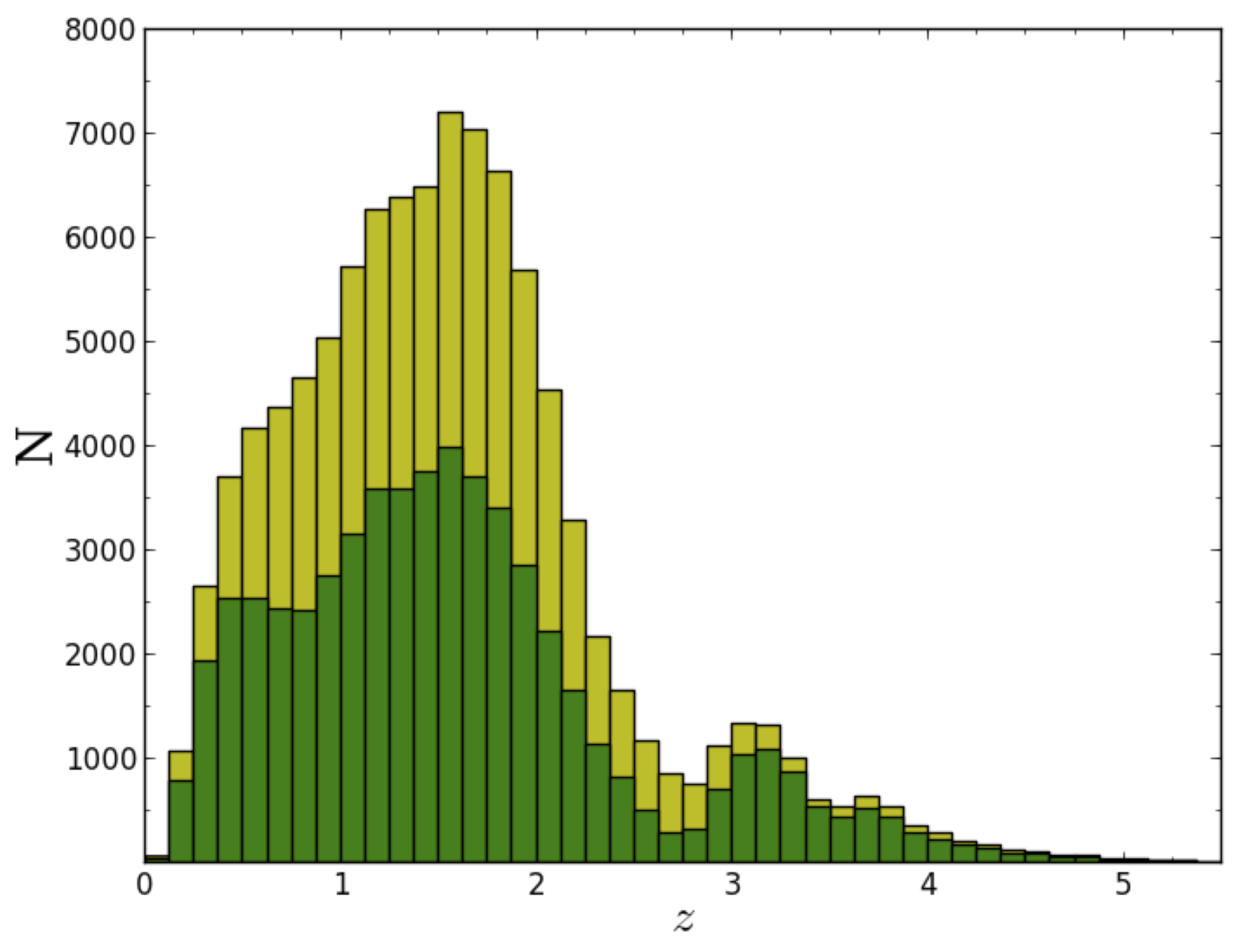
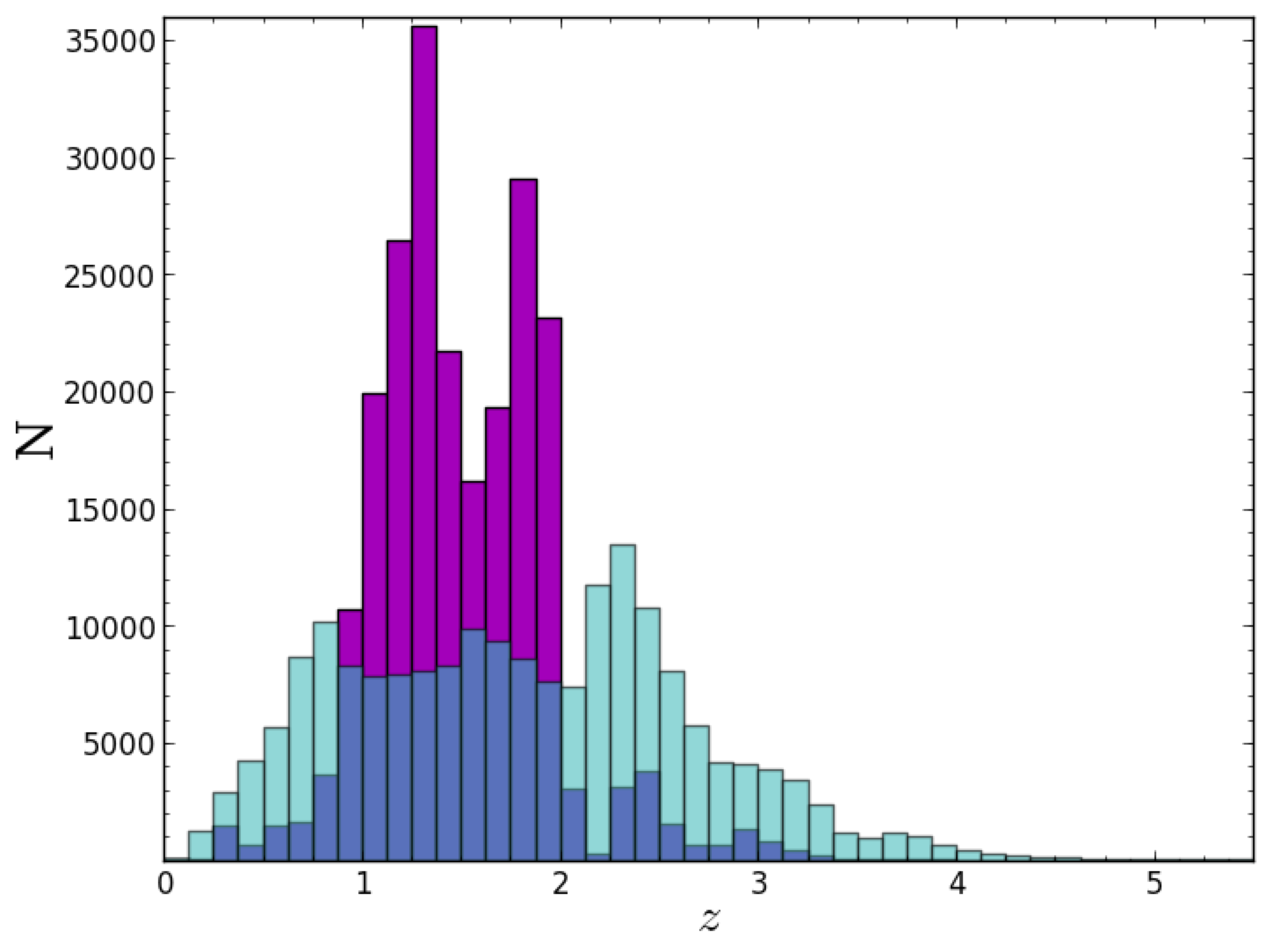
Figure 1: Histograms of the redshift distribution for Sample A (left; yellow; 93,362 quasars), Sample B (left; green; 55,302 quasars), Sample C (right; blue; 181,720 quasars), and Sample D (right; purple; 210,825 quasars). Note that the two plots use different y-axis scalings. Sample C fills in the redshift distribution gap seen near $z\sim 2.7$ in Samples A and B, while Sample D vastly increases the sample size by probing deeper than the spectroscopic samples (A,B,C) at the expense of the redshift distribution (and redshift accuracy).

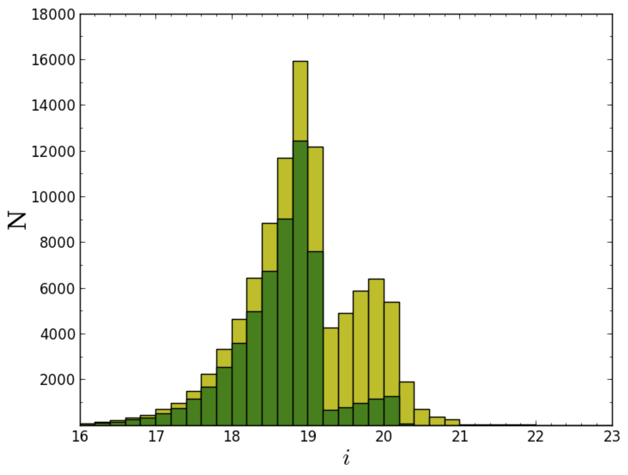
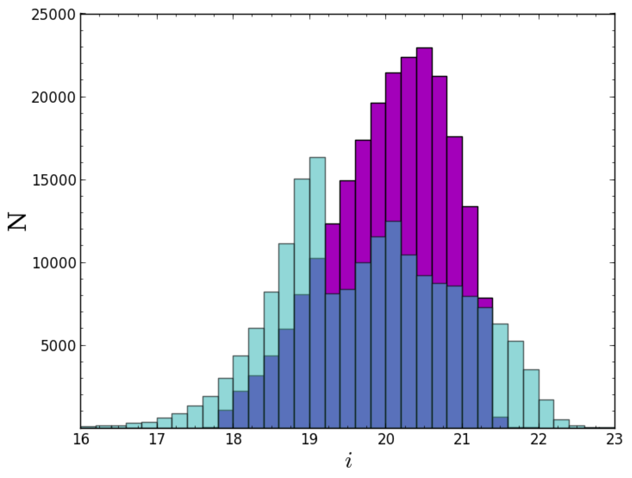
Figure 2: Histograms of the $i$-band magnitude distribution for all four samples (as outlined in Fig. 1). Again, note that the two plots use different y-axis scalings. The distribution of Sample A (left; yellow) reflects the different limiting magnitudes for $z<3$ and $z>3$ quasar selections in SDSS. Sample C (right; blue) demonstrates the extension to fainter magnitudes by the SDSS-III BOSS quasars, while Sample D (right; purple) probes more faint objects (while eliminating brighter objects where the efficiency of photometric quasar selection is lower due to higher stellar density).

2.6 Diagnostics

We present diagnostics of the radio and optical properties of our quasar samples as they relate to determining how any biases might complicate our understanding of the physics of quasar radio emission through better demographical analyses. These analyses have been performed on all four samples that we defined above, but results will only be shown for Samples B and D. Based on this analysis, we will limit our discussion in Section 4 to Sample B, noting where the other samples provide additional information.

2.6.1 Optical Luminosity and Redshift

Figure 3 shows the relationship between redshift and $K$-corrected $L_{2500\,\rm{\AA}}$ for Samples B and D. Two issues arise with regard to these parameters. First is the flux-limited nature inherent to blind surveys: because of our samples’ fixed magnitude limits, there is an inherent degeneracy between the redshifts and luminosities of the objects in our samples. Thus, some caution is needed to ensure that, for example, an observed characteristic of high-luminosity objects is not instead an inherent characteristic of high-redshift objects. As such, in our analyses in Section 4.1, we will consider the radio-loudness of quasars as a function of both properties simultaneously.

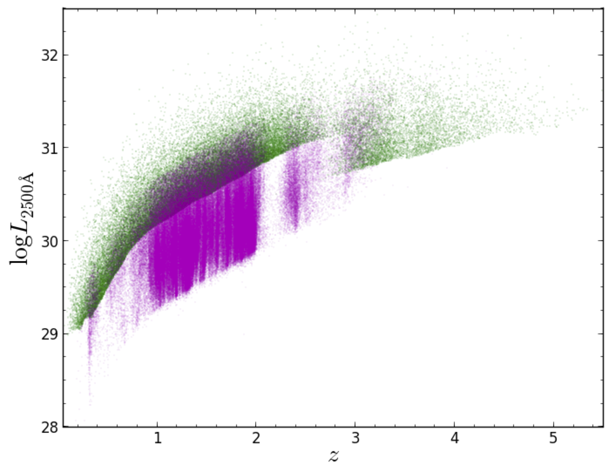
Figure 3: $L_{2500\,\rm{\AA}}$ corrected to $z=2$ as a function of redshift. The cuts made to Sample A to create Sample B (green; 55k quasars) has the effect of removing the faintest sources with $z<3$. After making cuts to Sample D (purple; 210k quasars) to create a relatively uniform subsample, photometric redshift degeneracies manifest themselves as bands of missing objects.

The optical luminosity itself is subject to its own corrections. Specifically, $K$-corrections need to be applied to ensure that we are comparing fluxes emitted in the same rest-frame wavelength range as opposed to fluxes received in the same observed-frame wavelength range. Traditionally, $K$-corrections are applied to extrapolate the power emitted by the object in its rest frame within the filter’s bandpass. Richards et al. (2006), adopting Wisotzki (2000) and Blanton et al. (2003), argue against $K$-correcting to $z=0$ since most quasars are not found in the local universe. To decrease the errors associated with extrapolating from high redshift objects to $z=0$, we follow Richards et al. (2006) and $K$-correct closer to the median redshift of our samples, $z=2$.

Lastly, we consider the redshift differences between the subsamples (as seen in both Figures 1 and 3). Sample B extends to $z\approx 5.5$ with $29<\log{L_{2500\,\rm\AA}}<33$, where the uniform restriction means that faint sources with $z<2.7$ have been removed. Sample D fills in at $z\sim 2.7$ and represents our efforts to create a larger, relatively uniform sample. However, we do so at the expense of certain redshift regions: the bands of missing objects in Sample D indicate where photometric redshift degeneracies exist.

2.6.2 Radio-Loudness

The standard definition of radio-loud is based on the ratio of radio to optical fluxes according to

$$R=\frac{f_{6\,\rm{cm}}}{f_{4400\,\rm{\AA}}},$$ (1)

where $f_{6\,\rm{cm}}$ is the 6 cm (5 GHz) measured radio flux, $f_{4400\,\rm{\AA}}$ is the $4400\,\rm{\AA}$ measured optical flux, and sources are considered radio-loud if $\log{R}>1$ (Schmidt, 1970; Kellermann et al., 1989). As emphasized by Ivezić et al. (2002, Section 4.2), the distribution of measured $\log{R}$ values can be significantly affected by both the optical and radio flux limits of a survey. As such, we examine these properties from our samples in Figure 4. In this plot, the total integrated radio flux (see Section 2.2) of each object is converted to a radio magnitude, $t$, in terms of the AB magnitude scale (Oke & Gunn, 1983). From Ivezić et al. (2002),

$$t=-2.5\log\left(\frac{f_{\rm int}}{3631\,\rm Jy}\right).$$ (2)

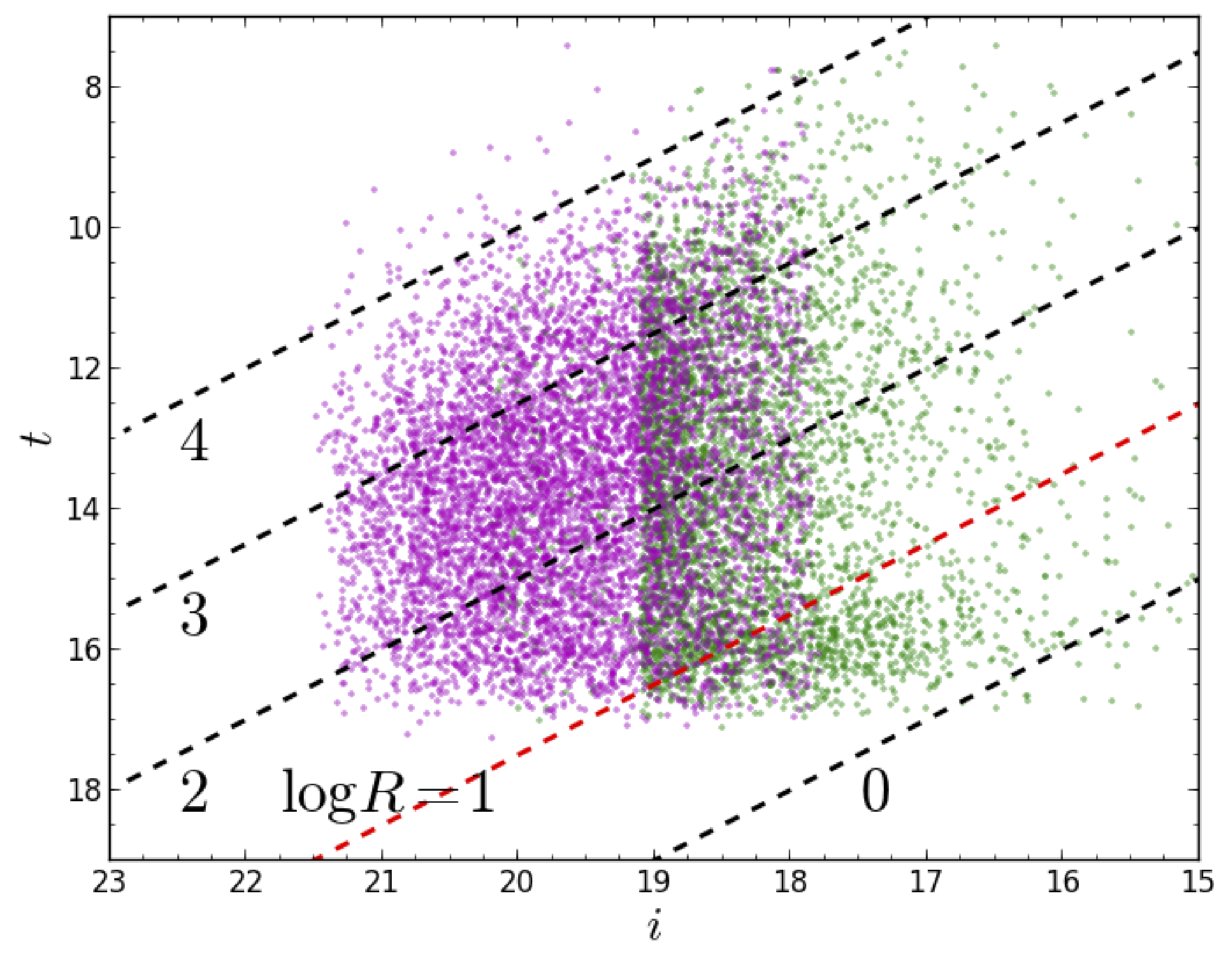
Figure 4: Radio magnitude ($t$) of detected FIRST sources as a function of $i$ (Sample B: green, 4590 quasars; Sample D: purple, 6580 quasars). The dashed diagonal lines represent different values of the radio-loudness parameter, $\log{R}$, with the boundary between RL and RQ, $\log{R}=1$, highlighted in red. It is apparent that the radio flux limit significantly restricts the distribution of $\log{R}$ to predominately RL values (for radio detected sources).

The maximum radio magnitude of $t=16.4$ corresponds to the 1 mJy detection limit of FIRST. The SDSS survey limits of $i=19.1$ (for low redshift) and $i=20.2$ (for high redshift) (Richards et al., 2002b) are readily seen in Sample B. The lines of constant $\log{R}$ show that these magnitude limits have a direct effect on the possible values of $\log{R}$ that can be measured for a given data set. For this reason, Ivezić et al. (2002) suggested exploring the histogram of $\log{R}$ values in a parameter space that runs perpendicular to the lines of $\log{R}$ within regions that are not bounded by the apparent magnitude limits (see Figure 19 of Ivezić et al. 2002). Note that only Sample B can be considered reasonably complete to radio-loud sources at the boundary of its optical flux limit ($i<19.1$).

Figure 5 illustrates a further limitation of the radio loudness parameter, $\log{R}$, by showing how it depends upon optical $i$-band magnitude. We calculated $\log R$ using Equation 1; if a particular object is within the FIRST observing area but has not been detected, $\log R$ is computed using the FIRST detection threshold flux of 1 mJy; this results in the artificial diagonal lines in the plots. The conventional division between RL and RQ ($\log R=1$; Kellermann et al. 1989) is plotted as a horizontal dashed gray line. Figure 5 illustrates that all of our samples exhibit RL incompleteness for objects fainter than $i\approx 18.9$. At fainter magnitudes, it is quite possible for an object to be intrinsically radio-loud but remain undetected by FIRST. On the other hand, objects brighter than $i=18.9$ that are not detected by FIRST should be classified as RQ even if they are eventually detected in the radio at a lower flux limit (modulo the incompleteness near the FIRST flux limits as discussed in Section 2.6.5). Our analysis of the RLF will concentrate on Sample B as both Figures 4 and 5 show that non-detections in the radio for Sample D could still be formally radio loud. A survey to 10$\times$ the depth of FIRST (or $\sim 15\,\mu$Jy at 20 cm) would be needed to detect all radio-loud quasars at the depth of SDSS photometry.

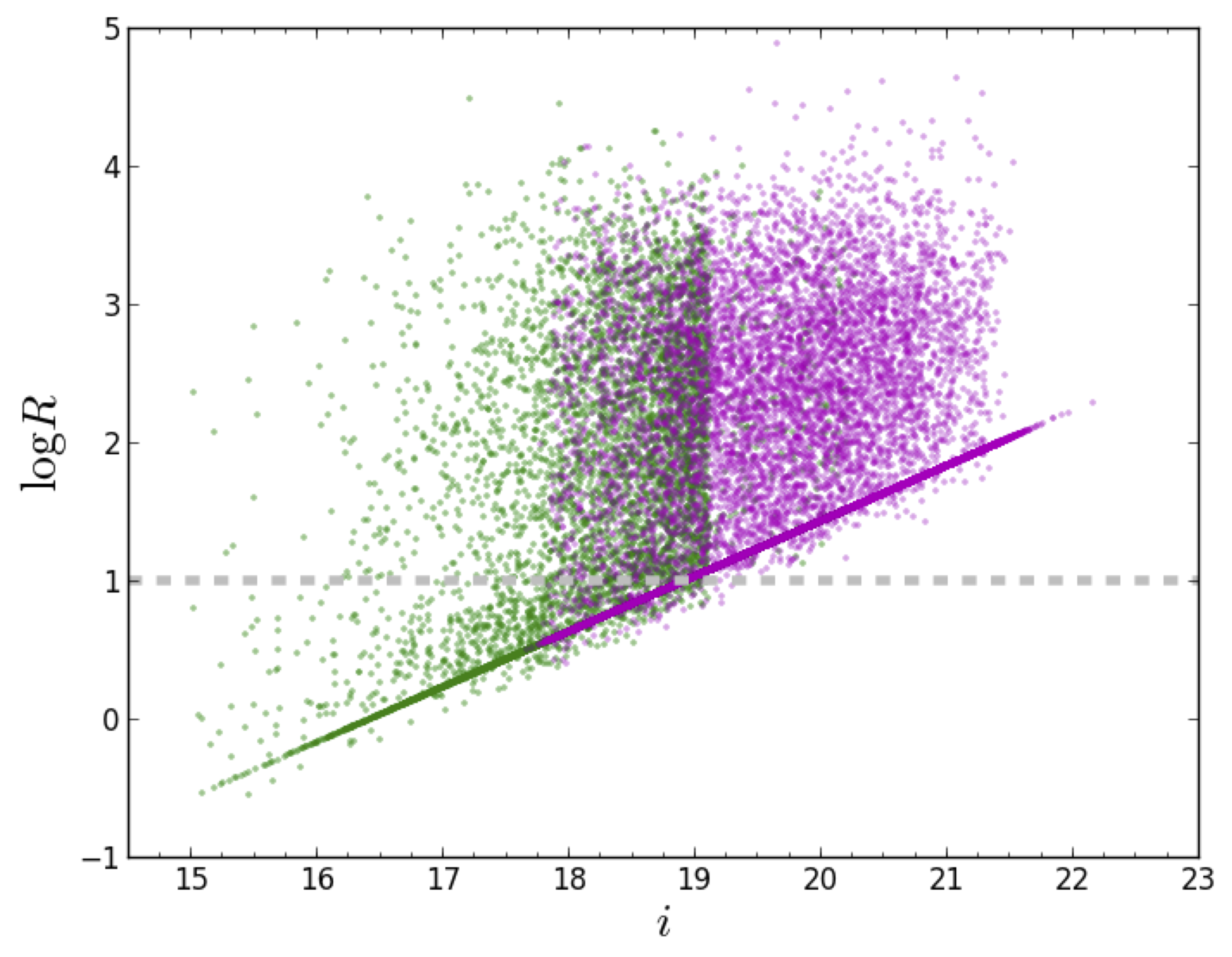
Figure 5: Radio-loudness, $\log R$, as a function of $i$ for optically confirmed quasars within the FIRST observing area (Sample B: green; Sample D: purple). Quasars undetected by FIRST are assigned a flux of 1 mJy to calculate $\log R$. Quasars undetected by FIRST at $i<18.9$ can be considered as RQ, but (optically) fainter objects can still be RL despite being undetected by FIRST.

2.6.3 Radio Luminosity

Using the ratio of radio and optical fluxes as a measure of radio loudness is preferred if those parameters are correlated. If, on the other hand, the radio and optical fluxes do not depend on one another, an absolute radio flux or power is a more significant boundary between RL and RQ quasars (Peacock et al., 1986; Miller et al., 1990; Ivezić et al., 2002); Goldschmidt et al. (1999) used $P_{5\rm GHz}=10^{24}$ W $\rm{Hz}^{-1}\,\rm{sr}^{-1}$ or $L_{20\rm cm}=10^{31}$ erg $\rm{s}^{-1}\,\rm{Hz}^{-1}$ as the limit between RL and RQ. As such, examination of the radio luminosity distributions leads to additional biases in our samples that must be considered. Figure 6 illustrates how radio luminosity depends on redshift for Samples B and D.

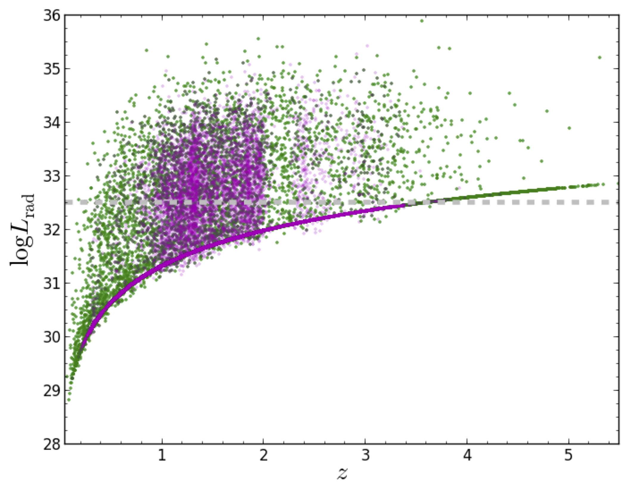
Figure 6: Radio luminosity as a function of redshift for optically confirmed quasars within the FIRST observing area (Sample B: green; Sample D: purple). Quasars undetected by FIRST are assigned a flux of 1 mJy to calculate $L_{\rm rad}$. The horizontal dashed gray line denotes a division between RL and RQ quasars employed by Jiang et al. (2007). It is evident that high-redshift quasars ($z\gtrsim 3.5$) can simultaneously be intrinsically radio-loud and FIRST non-detections. Alternatively, FIRST non-detections for lower redshifts ($z\lesssim 3.5$) strongly indicate that an object is RQ.

As with Figure 5, the FIRST flux limit is obvious in this plot and demarcates what redshifts (as opposed to fluxes) beyond which our sample is incomplete to radio-loud quasars. An alternate boundary (instead of $\log R$) between RL and RQ quasars utilized by Jiang et al. (2007), $L_{20\rm cm}=10^{32.5}$ erg $\rm{s}^{-1}\,\rm{cm}^{-2}\,\rm{Hz}^{-1}$, depends only on radio luminosity and is denoted with a horizontal dashed gray line. In all four samples, RL incompleteness exists above $z\gtrsim 3.5$. That is, as in Figure 5, it is possible for a high-redshift quasar to be intrinsically radio-loud, but still not be detected in FIRST. Thus, we should limit our most robust radio-loud fraction analysis to redshifts lower than this. On the other hand, a FIRST non-detection for lower redshifts is a strong indication that the object is radio-quiet. In Section 3.1 we will take advantage of this fact by treating FIRST non-detections (brighter than $i=18.9$ and with $z<3$) as confirmed RQ objects.

Furthermore, as with the optical, the spectral indices of quasars in the radio have a fairly large range, spanning at least $-1<\alpha_{\nu}<0$. Since our samples cover a large range of redshift, they must also span a large range of the rest-frame radio spectrum. As such, $K$-corrections to the rest-frame wavelength are important to consider. In a manner similar to $L_{2500\,\rm{\AA}}$ (see Figure 3), we follow Richards et al. (2006) and define an equivalently $z=2$ $K$-corrected radio luminosity as

$$\frac{L_{\rm{rad}}}{4\pi\,LD^{2}}=f_{\rm{int}}\,10^{-23}\,\frac{(1+2)^{\alpha_{\nu}}}{(1+z)^{(1+\alpha_{\nu})}}$$ (3)

where $L_{\rm{rad}}$ is measured in $\rm{erg}\,\rm{s}^{-1}\,\rm{Hz}^{-1}$, luminosity distance (LD) is measured in cm, integrated radio flux is measured in Jy, and the redshifts were taken from the optically detected objects. Here $\alpha_{\nu}$ is the radio spectral index, and we use $\alpha_{\nu}=-0.5$ for the entirety of this analysis as we have a combination of flat-spectrum ($\alpha_{\nu}\sim 0$) and steep-spectrum ($\alpha_{\nu}\sim-1$) sources in our samples. Kimball & Ivezić (2008) provide spectral indices for individual sources; however, non-simultaneity means that variability can skew the values. If simultaneous radio flux measurements in two bandpasses were available, it would be preferable to use radio spectral indices measured for each individual object. Figure 14 in Richards et al. (2006) illustrates how much error is induced by the wrong choice of spectral index, shows how the K-correction to $z=2$ serves to minimize that (for a population that peaks closer to $z=2$ than $z=0$), and suggests that an incorrect choice of spectral index should not have a large impact on our analyses. Note that this choice of $K$-correction means that any sample that uses the radio luminosity to define RL quasars will be biased towards including flatter spectrum (larger $\alpha$) sources at $z>2$ and steeper spectrum (more negative $\alpha$) sources at $z<2$.

2.6.4 Extended Flux Underestimation

A serious issue to consider when using integrated fluxes is that these measurements are underestimated for resolved FIRST sources ($>$ 10”) (Becker et al., 1995). The analysis by Jiang et al. (2007) ignores this possible complication, asserting that these highly extended radio sources are rare and so bright that, despite the underestimation of integrated flux, they will undoubtedly be considered RL.

One way to characterize this effect is to plot the ratio of the integrated to peak fluxes as a function of redshift. Here we use $\theta^{2}=(f_{\rm{int}}/f_{\rm{peak}})$ as defined by Ivezić et al. (2002), where $\theta>1$ for an extended source. In Figure 7, we see the effects of surface brightness dimming which goes as $(1+z)^{4}$. Some of the apparent fall-off with redshift is simply due to the declining number of sources, but it does appear that at the highest redshifts ($z\gtrsim 1.5$), extended sources are being preferentially lost. However, we emphasize that the (relatively) high frequency of the FIRST observations already biases the sample towards unresolved objects and reiterates the claim by Ivezić et al. (2002) that the fraction of complex sources is small within the FIRST sample. Thus, while we are not complete to quasars with extended radio emission, those objects are not dominating our sample, even at low redshift, and should not influence any trends with redshift. See the next section and both Bondi et al. (2008) and Hodge et al. (2011) for further discussion of resolution incompleteness.

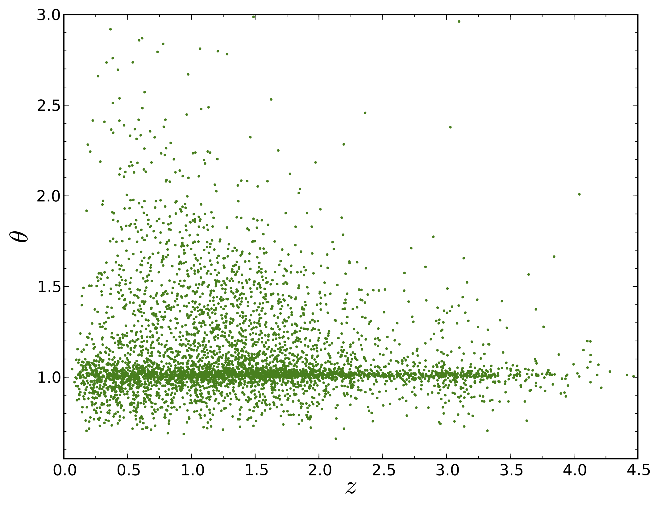
Figure 7: Source size, indicated by the ratio of the integrated to peak flux ($\theta$), as a function of redshift for FIRST-detected quasars in Sample B. Beyond $z=1.5$, the relative fraction of extended sources falls. However, this is not a large effect for our analysis as the majority of our sources are not resolved.

2.6.5 FIRST Detection Limit

Our final demographical analysis involves the FIRST detection limit, specifically how much this limit varies from the nominal limit of 1 mJy and why.

The depth to which FIRST can detect a source depends on sky position; being in the proximity of a bright object and the systematic increase in noise for lower declinations complicate FIRST’s sensitivity (Becker et al., 1995). In addition, the radio detection limit for FIRST is calculated using peak fluxes; this makes it difficult to accurately account for extended sources whose radio emission could be distributed throughout various components that may or may not exceed FIRST’s detection threshold (Becker et al., 1995; White et al., 2007). Therefore, the source counts with radio fluxes near the 1 mJy detection limit are incomplete, with extended sources being the most incomplete.

The completeness of FIRST is shown in Figure 8 as a function of integrated flux. The dots represent discrete values communicated by R. L. White (2013), and the solid line shows the linear fit between adjacent points that we used to interpolate completeness percentages. To compute the completeness efficiency, R.L. White (2013) used the measured size distribution of detected quasars. Based on this figure, we can see that FIRST suffers significant incompleteness above what is normally considered the “detection limit”.

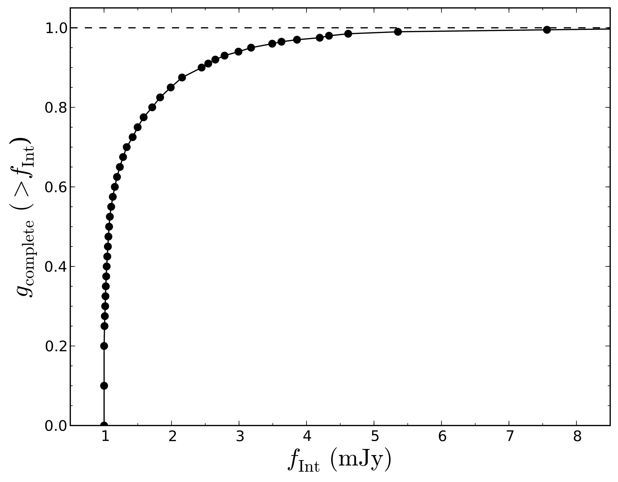
Figure 8: FIRST completeness (provided by R. L. White 2013, private communication) as a function of integrated radio flux (mJy). The incompleteness at the NVSS flux limit estimated here is consistent with that determined by Ivezić et al. (2002).

A concern is that any analysis probing to fluxes close to the nominal detection limit will suffer due to the relative uncertainty of the incompleteness correction near the limit. That said, Ivezić et al. (2002, Section 3.9) found that FIRST is not more than 13% incomplete at the NVSS (NRAO VLA Sky Survey; Condon et al. 1998) flux limit of $\sim$2.5 mJy, which is consistent with Figure 8. We will further discuss how this incompleteness could affect our results in Section 3.1.

2.7 Radio-Loud Definition

Before we begin our analysis of the data, it is worthwhile to review the mean spectral energy distribution (SED) of quasars and to consider the definition of a radio-loud quasar in the context of the broader quasar SED. Figure 9 shows multiple quasar SEDs to help illustrate the difference between RL and RQ. A radio-loud definition based on luminosity would mean simply making a cut along some constant value of the $y$-axis. A typical value would be at $\log L_{\rm rad}=32.5$ ergs $\rm{s}^{-1}\,\rm{Hz}^{-1}$. However, as discussed by Ivezić et al. (2002, Appendix C) and Baloković et al. (2012), the radio luminosity is the best indicator of radio-loudness only if the radio and optical luminosities are not correlated. As Baloković et al. (2012) demonstrates that these properties are indeed correlated, it means that it is arguably more appropriate to consider the ratio of the radio and optical luminosities.

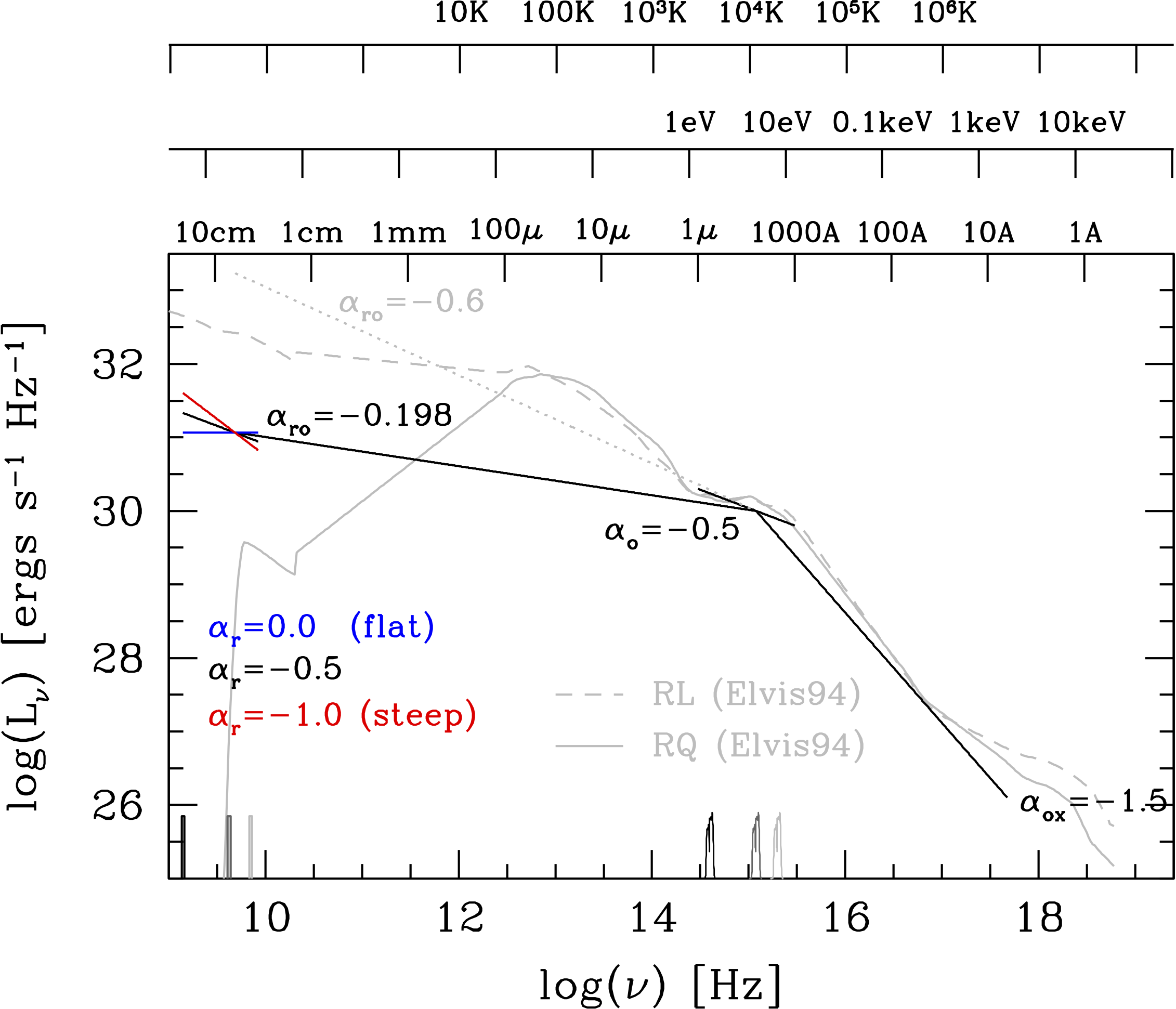
Figure 9: Spectral energy diagram comparing the distribution of power in the radio, optical, and X-ray regimes. The black lines show the mean radio-to-UV-to-X-ray SED of a quasar with $L_{2500\,\rm{\AA}}$ $=30$ ergs $\rm{s}^{-1}\,\rm{Hz}^{-1}$. $\alpha_{\rm{ro}}\,$ and $\alpha_{\rm{ox}}\,$ give the slope of the SED between the radio and optical and the optical and X-ray. $\alpha_{\rm{ro}}\,$ is not universal for quasars; here we have shown the slope corresponding to the traditional division between RL (steeper slopes) and RQ (flatter slopes). The red and blue lines show the range of radio slopes in that part of the SED. The solid and dashed gray curves show the mean RQ and mean RL SEDs, respectively, from Elvis et al. (1994). The dotted gray line shows a slope equivalent to $\log R=3$—particularly radio-loud. At the bottom of the panel we show the transmission of the 1.4GHz and i-band bandpasses at $z=0$, 2, and 4 (as black, dark gray, and light gray, respectively), demonstrating that, at $z=2$, the 1.4GHz and i-band bandpasses are close to 5GHz and $2500$Å.

Indeed, as noted above, the most common criterion used to classify quasars as RL or RQ is the $R$ parameter (Kellermann et al., 1989), which is just the ratio of the radio (6 cm) and optical (4400 $\rm\AA$) fluxes. While $R$ and $\log R$ (Ivezić et al., 2002) have a long history in the literature and are familiar to radio astronomers, the quasar field has become much more dependent on multi-wavelength data. As such, it is important to adopt terminology that is not specific to certain wavebands (e.g., $\log R$ in the radio or the energy index, $\Gamma$, in the X-ray), but rather terminology that spans the entire electromagnetic spectrum. Given the common usage of units that are related to ergs $\rm{s}^{-1}\,\rm{cm}^{-2}\,\rm{Hz}^{-1}$, a logical choice is the slope in $\log f_{\nu}$ vs. $\log\nu$ space, $\alpha$, where $f_{\nu}\propto\nu^{\alpha}$ (as shown in Figure 9, except in luminosity units).

In our work we will consider the radio-to-optical spectral index, $\alpha_{\rm{ro}}\,$, rather than $\log R$, where we define $\alpha_{\rm{ro}}\,$ according to

$$\alpha_{\rm ro}=\frac{\log(f_{\rm 5\,GHz}/f_{\rm 2500\,\AA})}{\log(\nu_{\rm 5\,GHz}/\nu_{\rm 2500\,\AA})}=\frac{\log(f_{\rm 5\,GHz}/f_{\rm 2500\,\AA})}{\log(\lambda_{\rm 2500\,\AA}/\lambda_{\rm 5\,GHz})}=-0.186\log(f_{\rm 5\,GHz}/f_{\rm 2500\,\AA}),$$ (4)

or more practically by considering the ratio of radio luminosity to optical luminosity. We have chosen the wavelength of $2500$ Å because it is the same as is used in X-ray investigations for comparisons with the optical/UV and represents the $i$-band at $z=2$. We have also chosen the frequency of 5 GHz because it is the historical value used in the radio and roughly corresponds to the frequency of the 1.4GHz (20 cm) FIRST data at $z=2$ (see below).

The values of $\alpha_{\rm ro}$ and $\log R$ are effectively equivalent if the frequencies sampled are the same, but using a slope (rise over run) instead of just the flux ratio (rise only) allows the use of data at other wavelengths/frequencies without having to apply significant corrections. In other words, $\alpha_{\rm ro}$ is more flexible than $\log R$. For the sake of backwards compatibility with previous work, the radio-to-optical spectral index, $\alpha_{\rm ro}$, can be related to the traditional $\log R$ parameter as follows (e.g. Wu et al., 2012):

$$R=\frac{f_{\rm 5\,GHz}}{f_{\rm 4400\,\AA}}$$ (5)

where

$$\frac{f_{\rm 5\,GHz}}{f_{\rm 2500\,\AA}}=\frac{f_{\rm 5\,GHz}}{f_{\rm 4400\,\AA}}\frac{f_{\rm 4400\,\AA}}{f_{\rm 2500\,\AA}}$$ (6)

and

$$\frac{f_{\rm 4400\,\AA}}{f_{\rm 2500\,\AA}}=\left(\frac{\nu_{\rm 4400\,\AA}}{\nu_{\rm 2500\,\AA}}\right)^{\alpha_{\rm opt}}=\left(\frac{\lambda_{\rm 2500\,\AA}}{\lambda_{\rm 4400\,\AA}}\right)^{\alpha_{\rm opt}}$$ (7)

so that

$$\alpha_{\rm ro}=\frac{\log\left[R\left(\frac{\lambda_{\rm 2500\,\AA}}{\lambda_{\rm 4400\,\AA}}\right)^{\alpha_{\rm opt}}\right]}{\log(\nu_{\rm 5\,GHz}/\nu_{\rm 2500\,\AA})}$$ (8)

which simplifies to

$$\alpha_{\rm ro}=-0.186\left[\log R+\alpha_{\rm opt}\log\left(\frac{\lambda_{\rm 2500\,\AA}}{\lambda_{\rm 4400\,\AA}}\right)\right]=-0.186\left[\log R-0.246\alpha_{\rm opt}\right].$$ (9)

For the mean optical spectral index from Vanden Berk et al. (2001) ($\alpha_{\rm opt}=-0.44$, needed to extrapolate between 2500Å and 4000Å) this corresponds to

$$\alpha_{\rm ro}=-0.186\log R-0.020.$$ (10)

To help calibrate $\alpha_{\rm ro}$ to the $\log R$ system, it may help to note that the traditional loud-quiet division ($\log R=1$) would be roughly $\alpha_{\rm ro}=-0.2$ and that $\alpha_{\rm ro}=-0.6$ would correspond to a very radio-loud source ($\log{R}\sim 3$).

Throughout the rest of this work we will assume that the radio and optical luminosities of quasars are correlated and, as such, will use the radio-to-optical flux ratio as given by $\alpha_{\rm ro}$ (rather than $\log R$) to distinguish between RL and RQ sources with $\alpha_{\rm ro}<-0.2$ as the definition for RL quasars.

3 Methods

Our analysis considers both the median radio properties of quasars (through a stacking analysis) and the extreme radio properties of quasars (using the fraction of objects in the radio-loud tail of the distribution). Here we explain in detail the methods used in these analyses before comparing the results of these two methods in Section 4.

3.1 Radio Properties in the Extreme: the Radio-Loud Fraction (RLF)

We begin our analysis by investigating the radio-loud fraction (RLF), which is the the percentage of quasars that have $\alpha_{\rm ro}<-0.2$ ($\log R>1$). Jiang et al. (2007) used a sample of more than 30,000 quasars to determine that the RLF increases with decreasing redshift and increasing optical luminosity. Their results may mean that the amount of radio emission with respect to that of the optical may change as a function of these two parameters; however, it could also suggest that the population densities of RL and RQ quasars evolve with respect to one another.

Jiang et al. (2007) showed that examining the RLF in 2-D $L-z$ space rather than the marginal distribution of $L$ and $z$ separately lead to very different results. We will perform the same analysis here with a larger, more uniform sample. Since redshift and luminosity are degenerate properties in flux-limited surveys, we divide our samples into equally populated bins within $L_{2500\,\rm{\AA}}$-$z$ space; this process allows us to isolate changes due to just one of the variables. Specifically, we first sort the quasars by redshift, dividing them into a number of slices with an equal population of quasars contained within each slice. Then we sort the objects in each redshift slice by luminosity and further bin the objects so that there are an equal number of objects in each $L-z$ bin. Quasars within a bin were flagged RL if $\alpha_{\rm{ro}}\,$ $<-0.2$, and, initially, the RLF for each bin was calculated by dividing the number of RL quasars by the total number of objects for that bin; see Figure 10 (left). The median $z$ and $L_{2500\,\rm{\AA}}$ for each bin were used to plot the results, and the color of each bin represents the RLF.

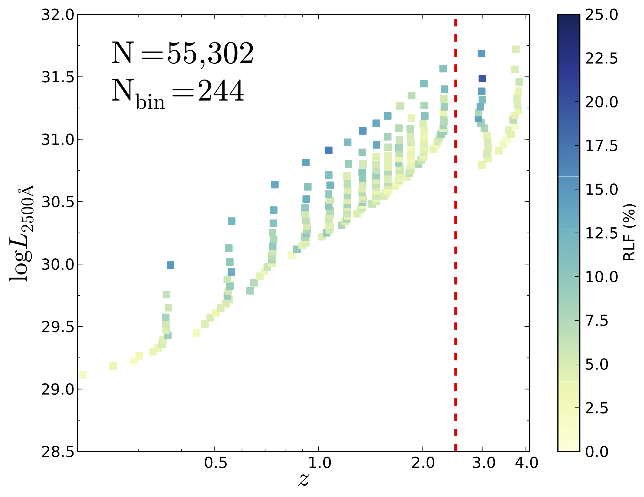
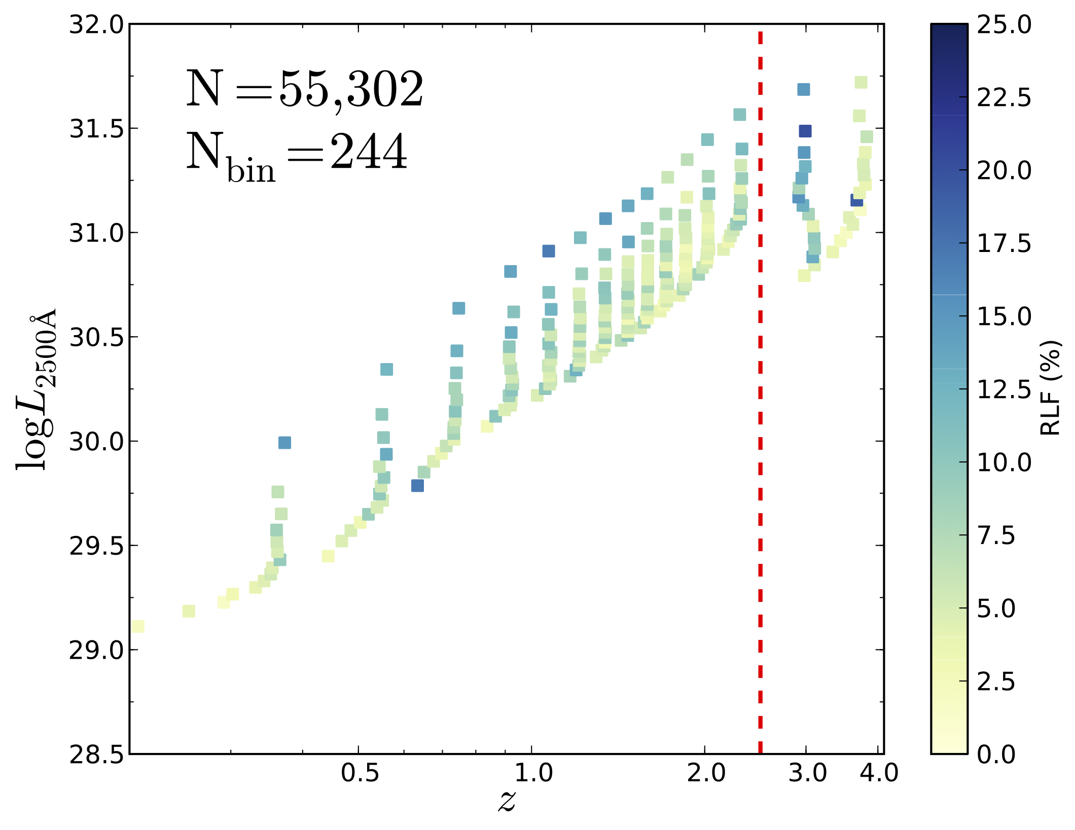
Figure 10: RLF as a function of both $L_{2500\,\rm{\AA}}$ and redshift for optically detected quasars within the FIRST observing area from Sample B. The plot on the left uses no correction when computing the number of RL objects within a bin, while the plot to the right uses the RL completeness correction (see Figure 8). Comparing the two, both plots show a declining RLF with increasing redshift and decreasing luminosity with the completeness corrected version (right) showing a less pronounced, yet still present, trend. The data to the right of the dashed red lines in both plots suffer the most from selection effects.

In order to correct for the incompleteness discussed in Section 2.6.5, we weigh each RL quasar that has a measured integrated flux less than 10 mJy by its corresponding completeness on our best fit function (Figure 8; solid line). For example, a RL object with an integrated radio flux of 1.075 mJy ($g_{\rm complete}=0.500$) counts as two RL objects since $1/g_{\rm complete}=1/0.500=2$. Because the completeness function drops off so quickly for integrated fluxes less than 1 mJy, all detected RL objects with values smaller than this are scaled by $g_{\rm complete}=0.10$. RL quasars with integrated fluxes greater than or equal to 10 mJy always count as one RL object, and the total number of objects within each bin remains unchanged when computing the RLF.

The plot on the right of Figure 10 shows the dependence of the RLF on both redshift and $L_{2500\,\rm{\AA}}$ for Sample B after applying the completeness correction. We see that the trend in RLF from the upper-left to the lower-right is reduced but still present. Everything to the right of the vertical red line located at $z\sim 2.5$ in both plots denotes where the SDSS optical selection was very inefficient; further care is required to fully understand our analysis beyond this redshift. In short, the optical selection is less complete at this redshift (compare panels a and b in Richards et al. 2006, Fig. 6), so the quasars discovered at $z\sim 2.5$ are more likely to be radio sources.

This type of analysis allows us to see how the RLF is changing as a function of multiple parameters; we can then compare these results with the mean radio properties of quasars in order to see if the direction of change is the same for both methods. Our analysis in Section 4.1 starts with the $L-z$ plane as shown here. In later sections, we will construct similarly binned samples using other observed quantities, plotting some third parameter as a color-scale at the median value of the $x$ and $y$ quantities. Specifically, we also consider the C IV blueshift and equivalent width (EQW) (Section 4.2), the so-called “Eigenvector 1” parameter space (Section 4.2), and the combination of BH mass and accretion rate (Section 4.3).

3.2 Radio Properties in the Mean: Stacking Analysis

3.2.1 Image Stacking

By stacking the radio images of all known quasars covered by the FIRST survey, we hope to learn about the mean radio properties of these objects. We can then contrast these findings with the properties identified using formally radio-loud quasars. Our stacking analysis follows that of White et al. (2007). For a more detailed explanation, see that paper, but the process is briefly described here.

First, using the optical coordinates of our target quasar populations, 0$\farcm$5 x 0$\farcm$5 radio images were downloaded from the FIRST data extraction website. As with the RLF analysis, we wish to explore the mean radio characteristics of quasars as a function of various properties. As such we will stack the radio images in bins based on these parameter spaces (e.g., $L-z$, Section 4.1; CIV and EV1, Section 4.2; BH properties, Section 4.3; color, Section 4.4).

After assigning each quasar to a 2-D parameter bin, all of the FIRST radio images within each bin were added using a median stacking procedure (see White et al., 2007): a pixel in the final stacked image corresponds to the median value of the pixels occupying that same location from the set of radio images within a bin. Since White et al. (2007) show that the median converges to the mean for distributions such as we consider herein, we will generally refer to our median stacking results as the mean.

After combining the cutouts into stacked images, the peak flux values of our stacked sources need to be corrected for what White et al. (2007) designate as “snapshot bias”, which appears to be related to the well-known problem of “clean bias” associated with FIRST sources (Becker et al., 1995). White et al. (2007) found that a correction of the form:

$$f_{\rm peak,\,\mathrm{corr.}}=\mathrm{min}(1.40\,f_{\rm peak},\,f_{\rm peak}+0.25\;\mathrm{mJy}),$$ (11)

is needed, where $f_{\rm peak}$ is the peak flux density (mJy) of the median stack. The flux boundary that determines which part of the equation to implement is 625 $\mu$Jy. As that value is more than 200 $\mu$Jy greater than the largest median peak flux density we achieve, we will only need to multiply our measurements by 1.40 for the entirety of our analysis to correct for this bias.

3.2.2 Median Stacking Diagnostics

Before we can interpret the results of the stacking analysis, we must first understand what biases are inherent to the process by looking at some diagnostic information. We first explore the distribution of mean radio flux density by stacking in redshift bins (Figure 11), breaking Sample B (D) into 50 (100) redshift bins with 1116 (1981) quasars per bin. After applying the median stacking procedure described above, we get the same basic results as White et al. (2007): the median flux density declines up to $z=2$. This trend of decreasing flux density with redshift is expected based on inverse square law dimming. Note Sample B includes 10,000 more quasars than considered by White et al. (2007) (41,295 SDSS DR3 quasars) and should be clean of selection effects up to $z\sim 2.2$.

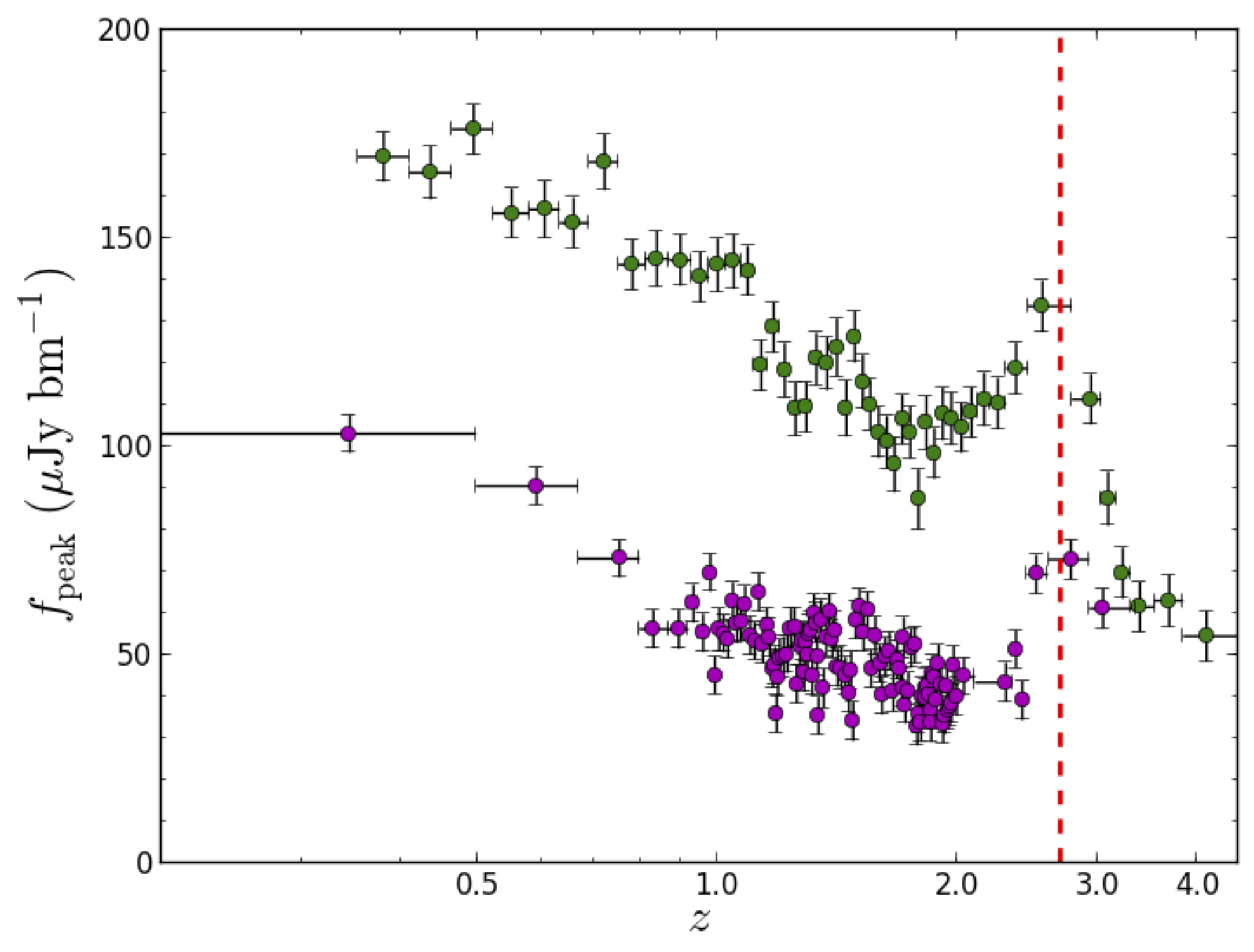
Figure 11: Peak flux density ($\mu$Jy bm^-1) of median stacked quasars as a function of redshift (see White et al., 2007, Fig. 6) (Sample B: green, 1116 quasars per point; Sample D: purple, 1981 quasars per point). The Sample D sources are fainter in the optical than the Sample B sources. The vertical dashed lines represent $z=2.7$, which is the upper limit of efficient SDSS optical selection.

We observe an increase in median flux density starting at roughly $z=2.2$ for all our samples (typically peaking at $z\sim 2.7$). This increase can be attributed to selection effects whereby the SDSS optical selection was very inefficient at $z\sim 2.7$ while the radio selection is more complete (compare panels a and b in Richards et al. 2006, Fig. 6). As such, the quasars discovered at $z\sim 2.7$ are more likely to be radio sources, thus biasing the observed mean flux and requiring that a robust analysis be limited to $z<2.2$.

We next investigate the mean radio flux density and $\alpha_{\rm{ro}}\,$ as a function of $i$-band magnitude to explore the correlation between radio and optical brightness. Figure 12 shows that the strongest radio emitters are also the optically brightest, while Figure 13 shows that the optically faintest sources are the most radio-loud, consistent with White et al. (2007, Figs. 7 and 12). These trends mean that, as for the RLF, some caution is needed in interpreting trends of radio properties that follow trends with apparent magnitude.

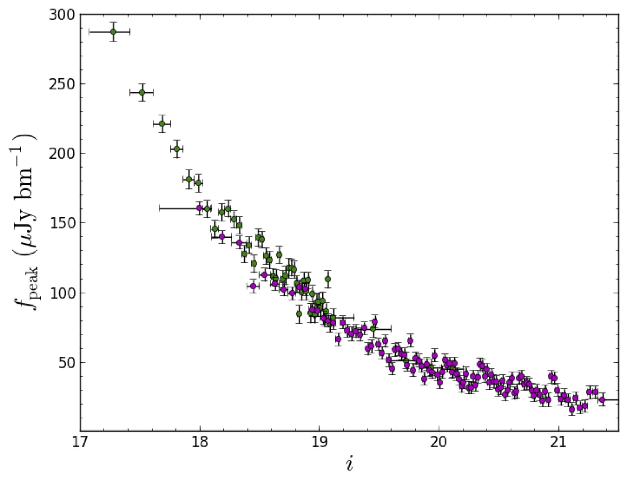
Figure 12: Peak flux density ($\mu$Jy bm^-1) of median stacked quasars as a function of $i$ band color (see White et al., 2007, Fig. 7) (Sample B: green; Sample D: purple). As before, the strongest radio emitters are associated with the optically brightest sources. This trend is consistent with dimming of both the radio and optical with increasing redshift.

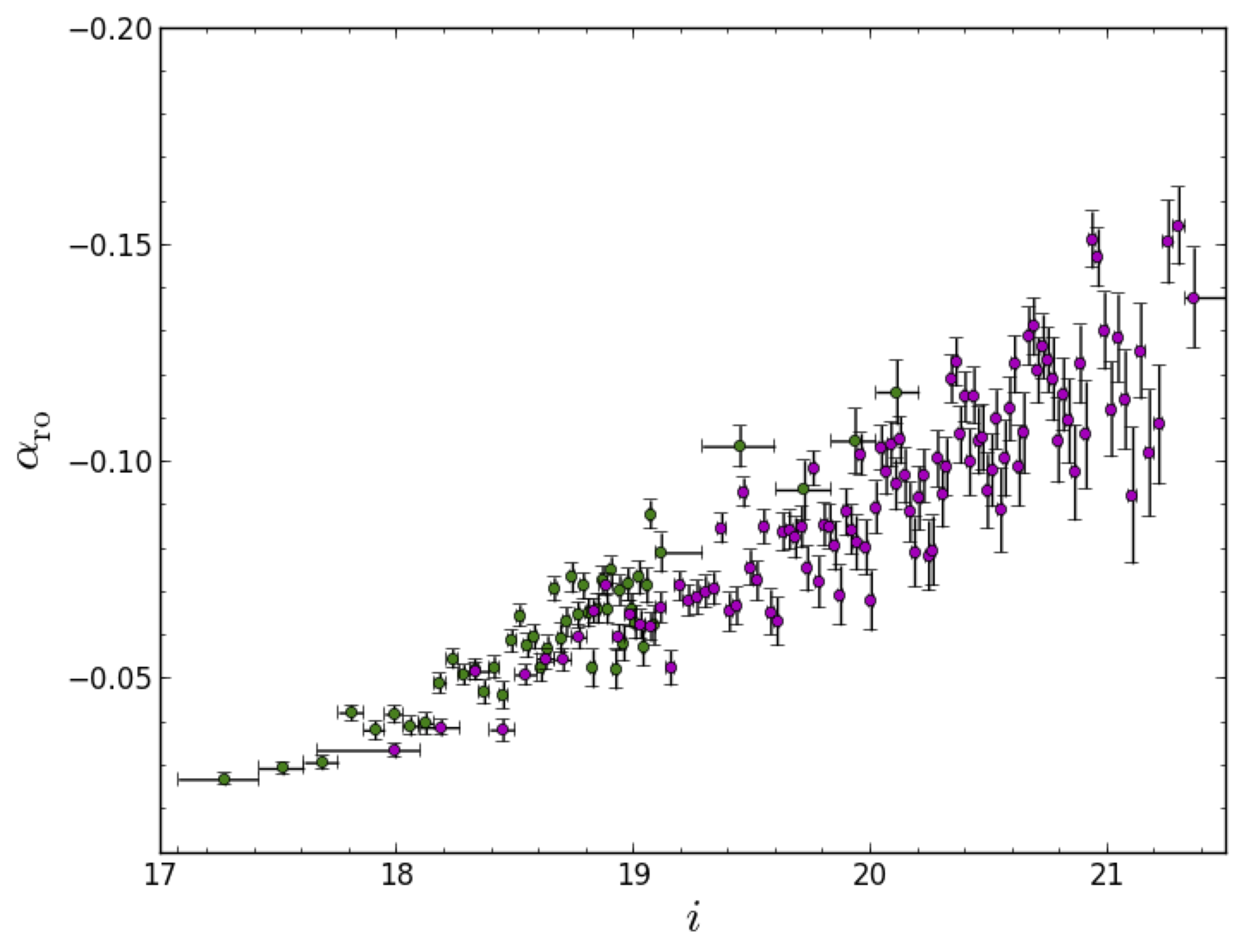
Figure 13: $\alpha_{\rm{ro}}\,$ of median stacked quasars as a function of $i$ band color (see White et al., 2007, Fig. 12) (Sample B: green; Sample D: purple). While Figure 12 showed that the brightest sources in the optical are the brightest in the radio, the ratio of radio to optical flux is such that the radio-loudest objects (more negative values of $\alpha_{\rm{ro}}\,$) are associated with the faintest optical sources.

3.2.3 Choice of Radio Loudness Metric

While the RLF is our metric for the extreme radio properties, we must decide what metric to use for comparison of the mean radio properties. We will conclude that the $\alpha_{\rm{ro}}\,$ is the parameter of choice. Knowing that, the reader can skip to Section 4 if desired; however, it is worth spending some time looking at the trends with radio flux and luminosity in $L-z$ parameter space and reviewing how we made the choice of $\alpha_{\rm{ro}}\,$ as our comparison metric before comparing the results to the RLF.

In Figure 14 we show the median radio flux density (colored squares) as a function of $L$ and $z$. Here we see that, at a fixed redshift, quasars that are optically more luminous have higher radio fluxes, and at a fixed optical luminosity, lower redshift quasars have higher radio fluxes. The trend is roughly consistent with the mean radio flux being primarily dependent on the optical magnitude: optically brighter quasars are radio brighter, on average; see also Figure 12.

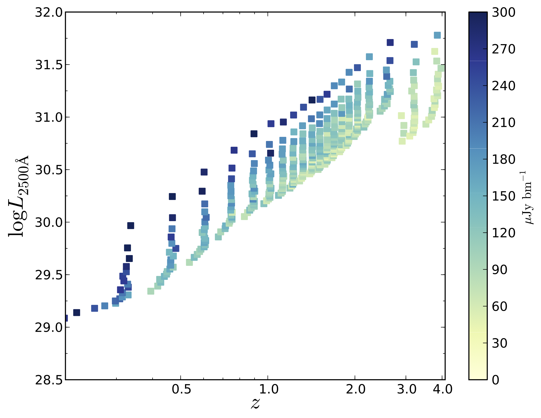
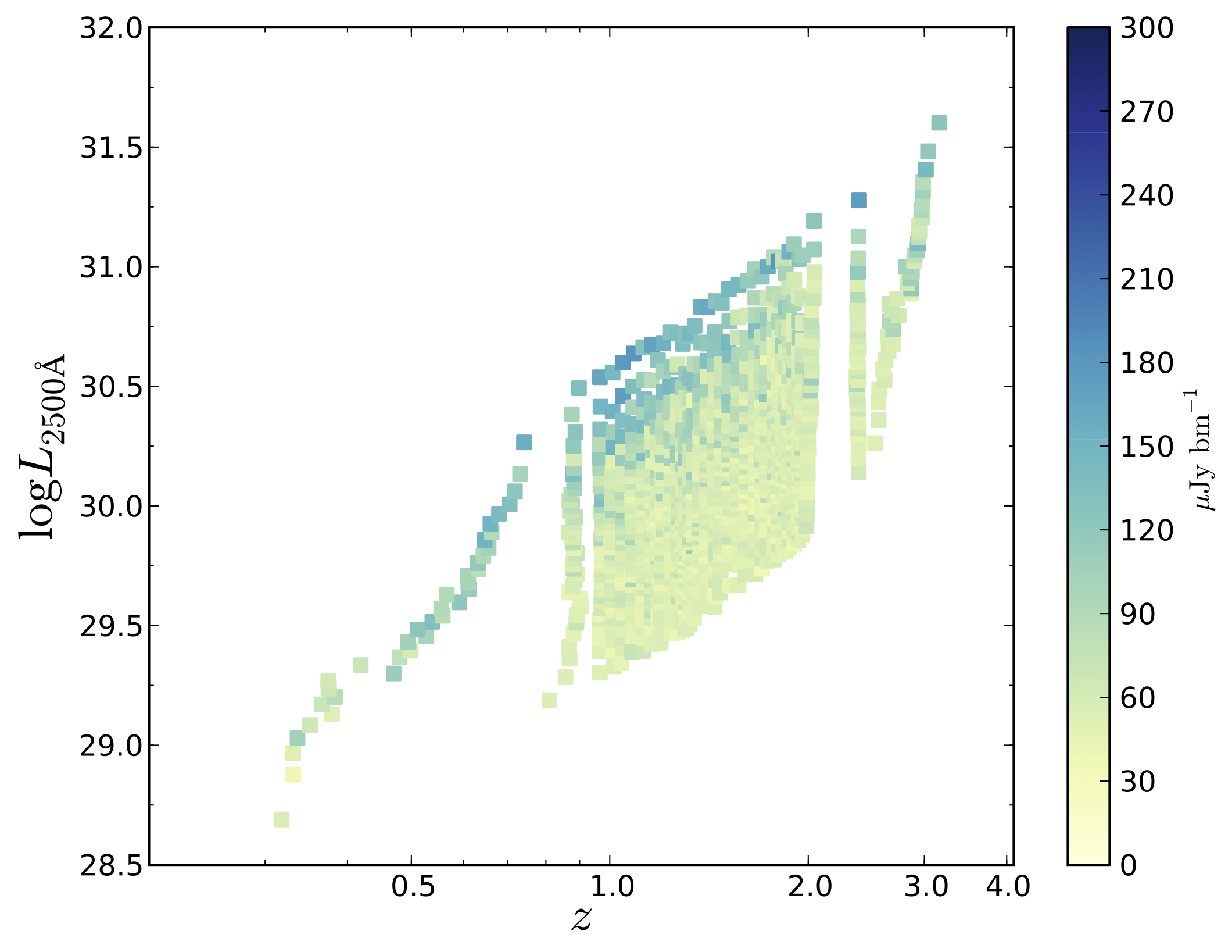
Figure 14: Peak flux density ($\mu$Jy) of median stacked quasars as a function of both redshift and $L_{2500\,\rm{\AA}}$. (Left:) Sample B, 138 objects per bin; (Right:) Sample D, 151 objects per bin. The trend roughly follows the $i$-band magnitude with brighter quasars in the optical being brighter in the radio.

Since we really want to understand the intrinsic radio properties, we now convert from apparent brightness to luminosity, where the conversion from radio flux to radio luminosity is determined according to Equation 3 as discussed in Section 2.6.3. Figure 15 shows the results of stacking the radio luminosities in the $L_{2500\,\rm{\AA}}$-$z$ plane. Again, more luminous sources in the optical tend to be more luminous in the radio, but a larger effect is seen with redshift, where a small radio flux at high-$z$ can translate to a high radio luminosity. The most radio luminous sources are at high-$z$ and have high optical luminosities. Objects with roughly equal radio luminosities span a diagonal from the upper-left to the lower-right while radio luminosity decreases from the upper-right to lower-left.

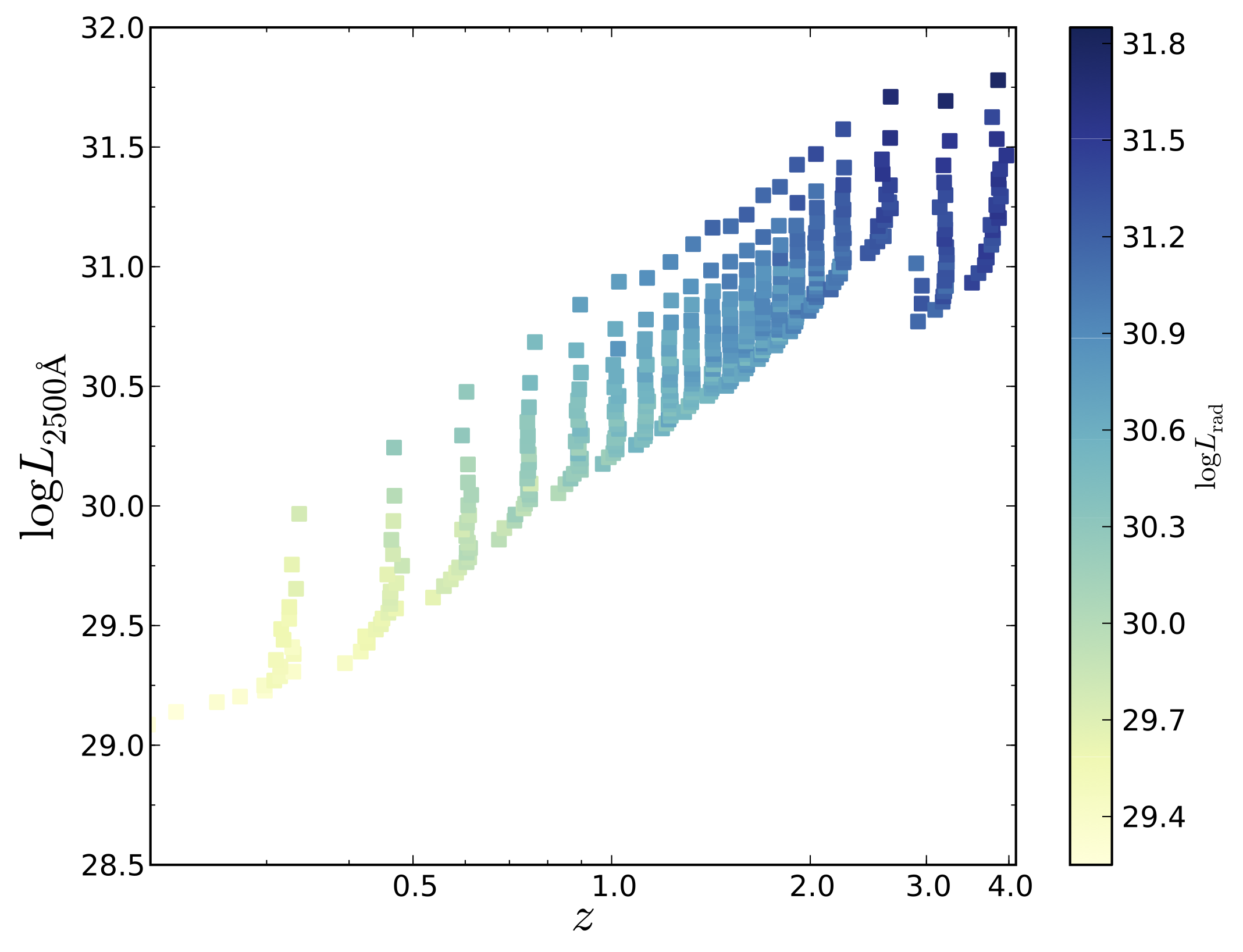
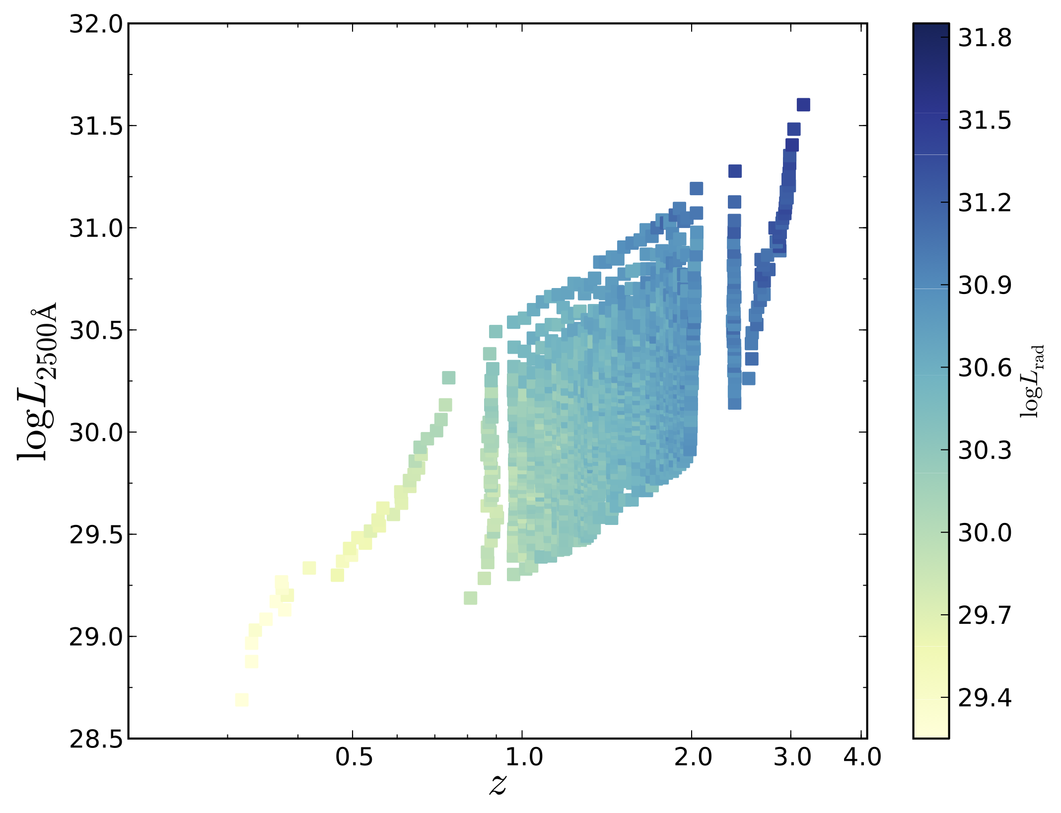
Figure 15: Radio luminosities ($\rm{erg}\,\rm{s}^{-1}\,\rm{Hz}^{-1}$) of median stacked quasars as a function of both redshift and $L_{2500\,\rm{\AA}}$. (Left:) Sample B; (Right:) Sample D. The bins are the same as those used in Figures 14. As expected, the most radio luminous sources are at high-$z$ and have high optical luminosities with radio luminosity decreasing from the upper-right to lower-left.

As noted in Section 2.7, looking at the radio luminosity as a measure of radio-loudness is correct only if there is no correlation between the optical and the radio. If there is a correlation, then it is more appropriate to consider the ratio of the two, or equivalently, the spectral index between the radio and optical, $\alpha_{\rm{ro}}\,$, which is defined in Section 2.7.

Figure 16 shows the resulting distribution in $\alpha_{\rm{ro}}\,$, which is a measure of the slope of the SED between the radio and optical. We see that normalizing by the optical luminosity has produced a significantly different trend than we saw in Figure 15. That trend is for quasars to be stronger radio sources (relative to the optical) with decreasing optical luminosity (at fixed redshift) and with increasing redshift (at fixed optical luminosity). This trend is perhaps unexpected but is indeed consistent with Figure 15, where we saw that equal radio luminosities occupied roughly diagonal tracks in $L_{2500\,\rm{\AA}}$-$z$ space. Along one of those diagonals, the objects with the lowest optical luminosity will have the largest radio-to-optical ratio, so we expect radio-dominance from the objects along the lower boundary of the distribution.

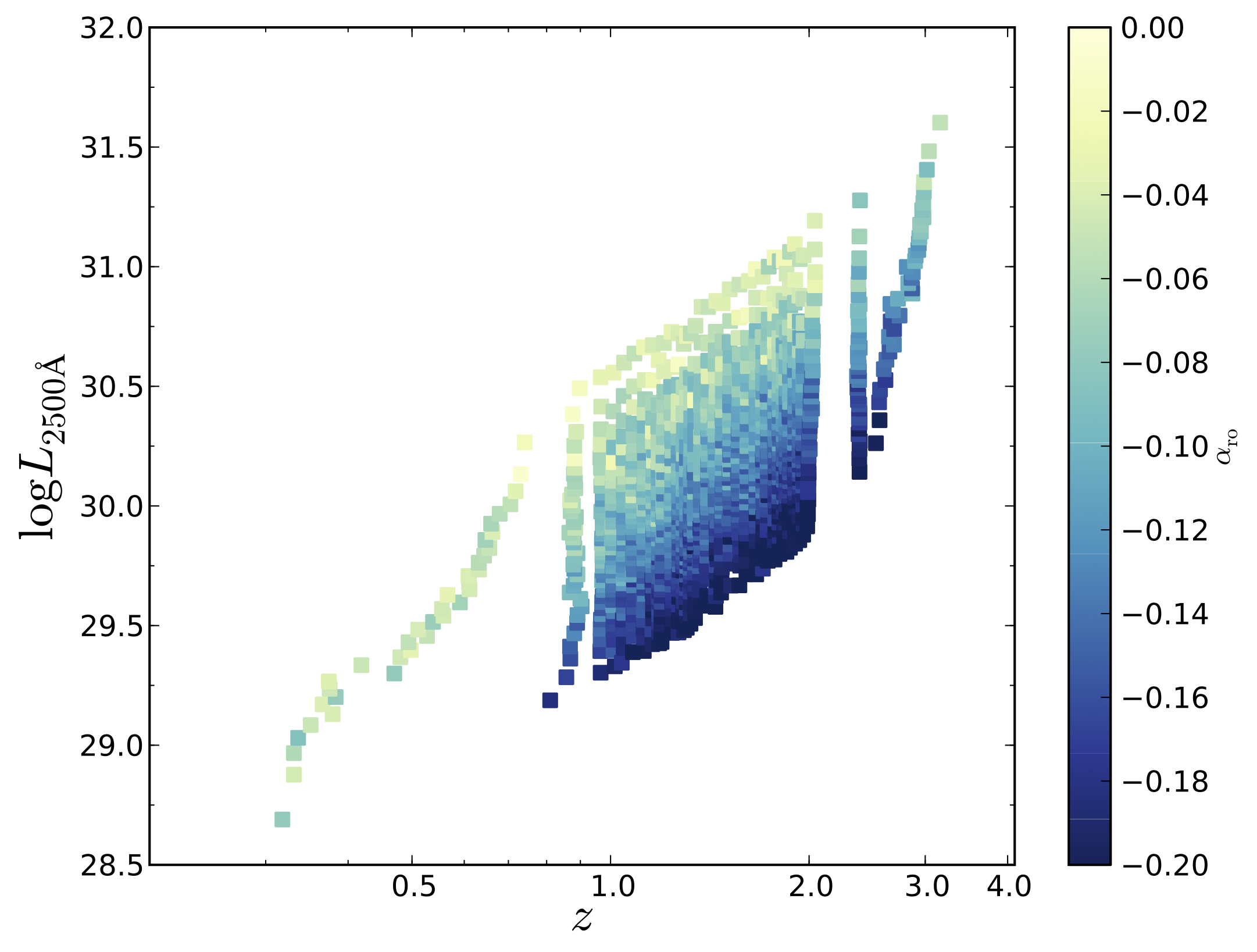
Figure 16: Radio to optical spectral indices ($\alpha_{\rm ro}$) of median stacked quasars as a function of both redshift and $L_{2500\,\rm{\AA}}$. (Left:) Sample B; (Right:) Sample D. These bins are the same as those used in Figures 14 and 15. This trend is completely opposite to that found for the RLF (see Figure 10). The median stacking shows stronger radio sources (relative to the optical) with decreasing optical luminosity (at fixed redshift) and with increasing redshift (at fixed optical luminosity).

As there is precedent for the slope of the spectral energy distribution in quasars to be a function of luminosity, it is also important to consider how $\alpha_{\rm{ro}}\,$ may change with $L_{2500\,\rm{\AA}}$. In particular, it has been repeatedly shown (e.g., Avni & Tananbaum, 1982; Steffen et al., 2006; Just et al., 2007; Lusso et al., 2010) that there is a non-linear relationship between the X-ray and UV luminosity in quasars: quasars with double the UV luminosity do not have double the X-ray luminosity. Failure to correct for any similar systematic trends in $\alpha_{\rm{ro}}\,$ with optical luminosity could lead to biased conclusions. As such we investigate the relationship between $L_{\rm rad}$ and $L_{\rm opt}$ in terms of the behavior of $\alpha_{\rm{ro}}\,$ as a function of $L_{2500\,\rm{\AA}}$ by separating the quasars into bins of optical luminosity with 1000 objects in each bin.

The top-left plot of Figure 17 shows the correlation between $L_{\rm rad}$ and $L_{2500\,\rm{\AA}}$ (see White et al., 2007, Fig. 9) for the entire range of redshifts within Sample B, whereas the other panels show restricted redshift ranges. Here it is important to have limited our analysis to Sample B as using a less homogeneous sample can imprint biases onto the distribution in $\alpha_{\rm{ro}}\,$-$L_{2500\,\rm{\AA}}$ parameter space. We have further limited our analysis to point sources to avoid contributions from the host galaxy to the optical luminosity and to $z<2.2$ to avoid the known bias towards radio sources in the SDSS selection function at higher redshifts.

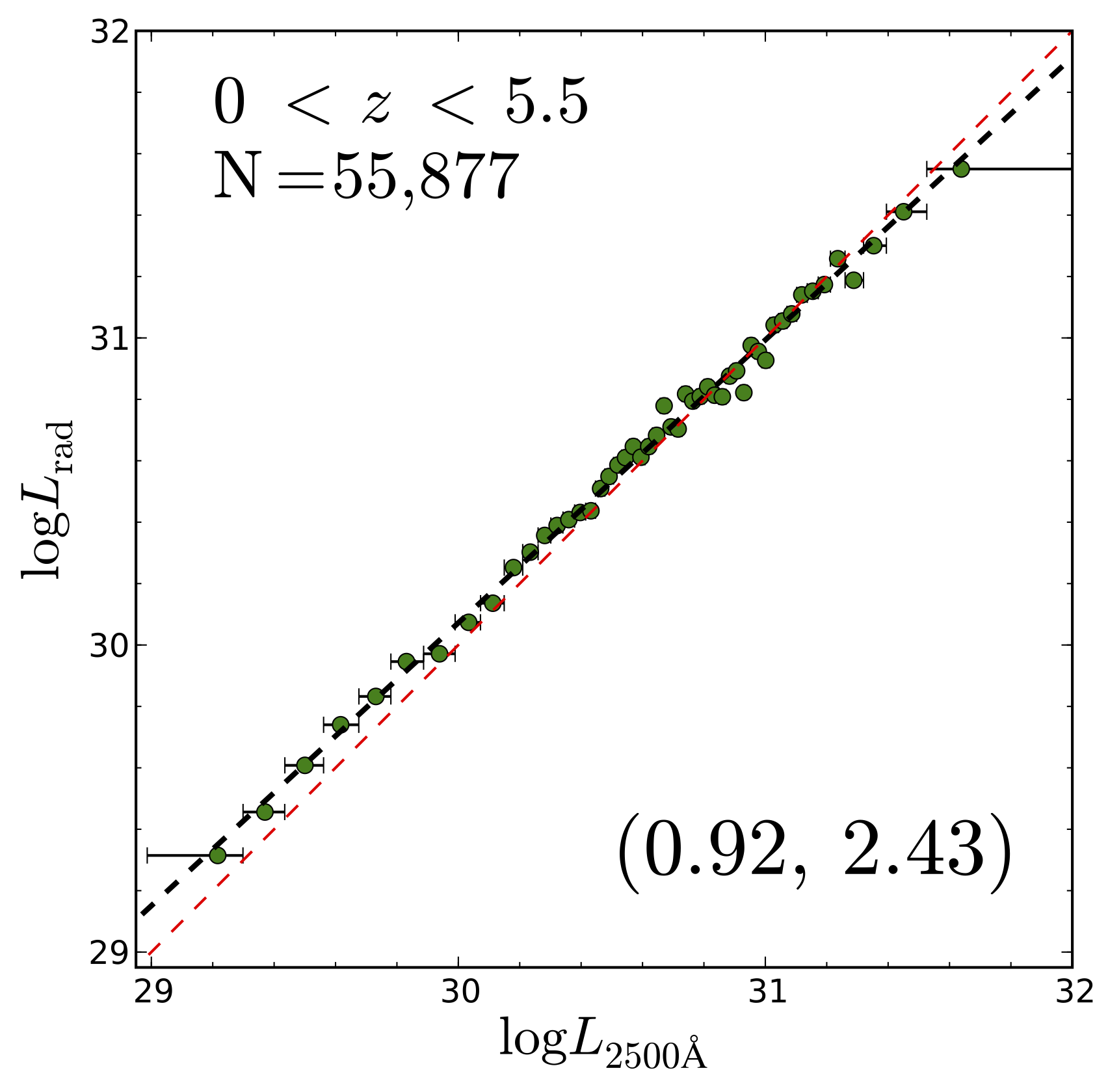
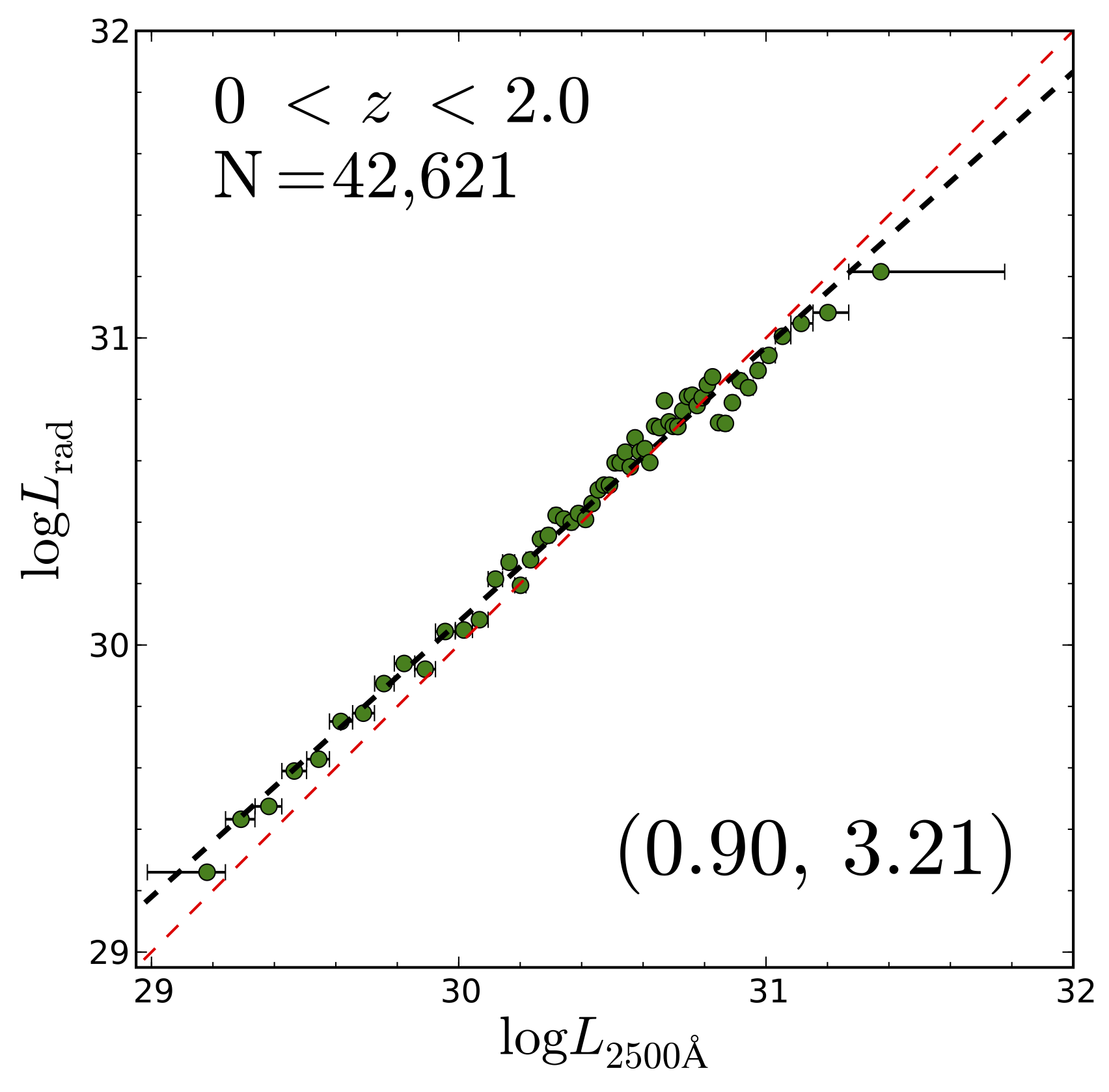
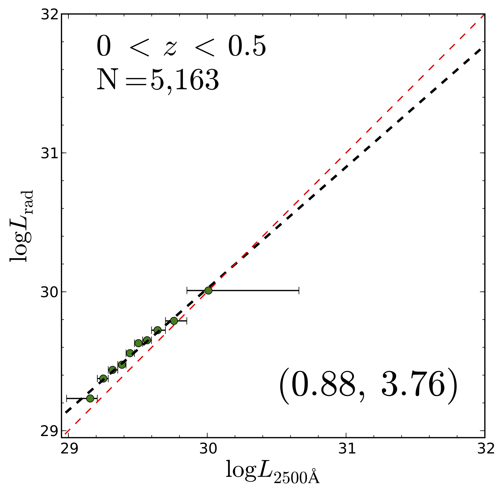
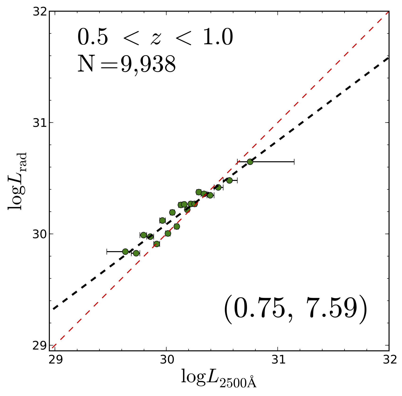
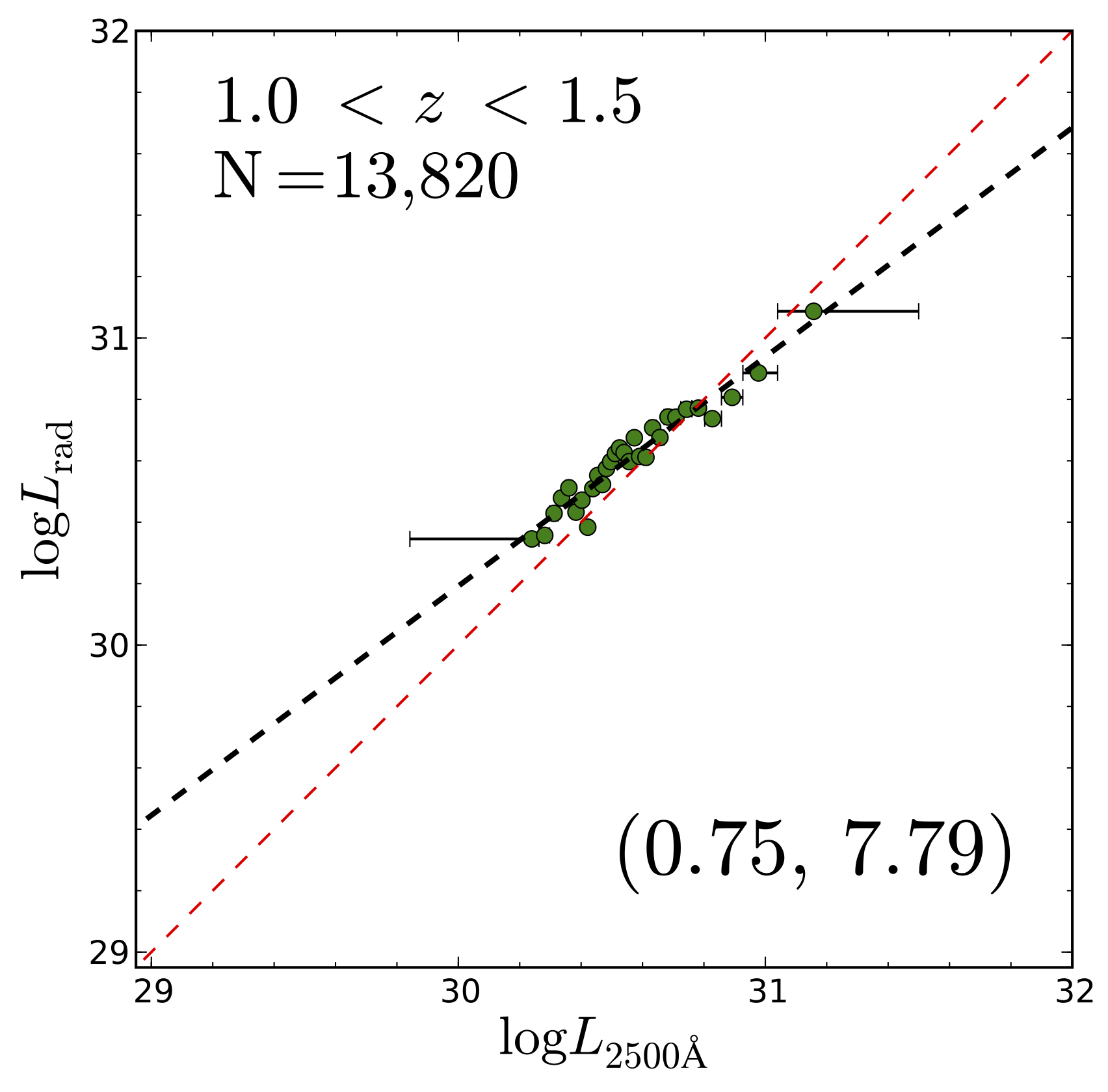
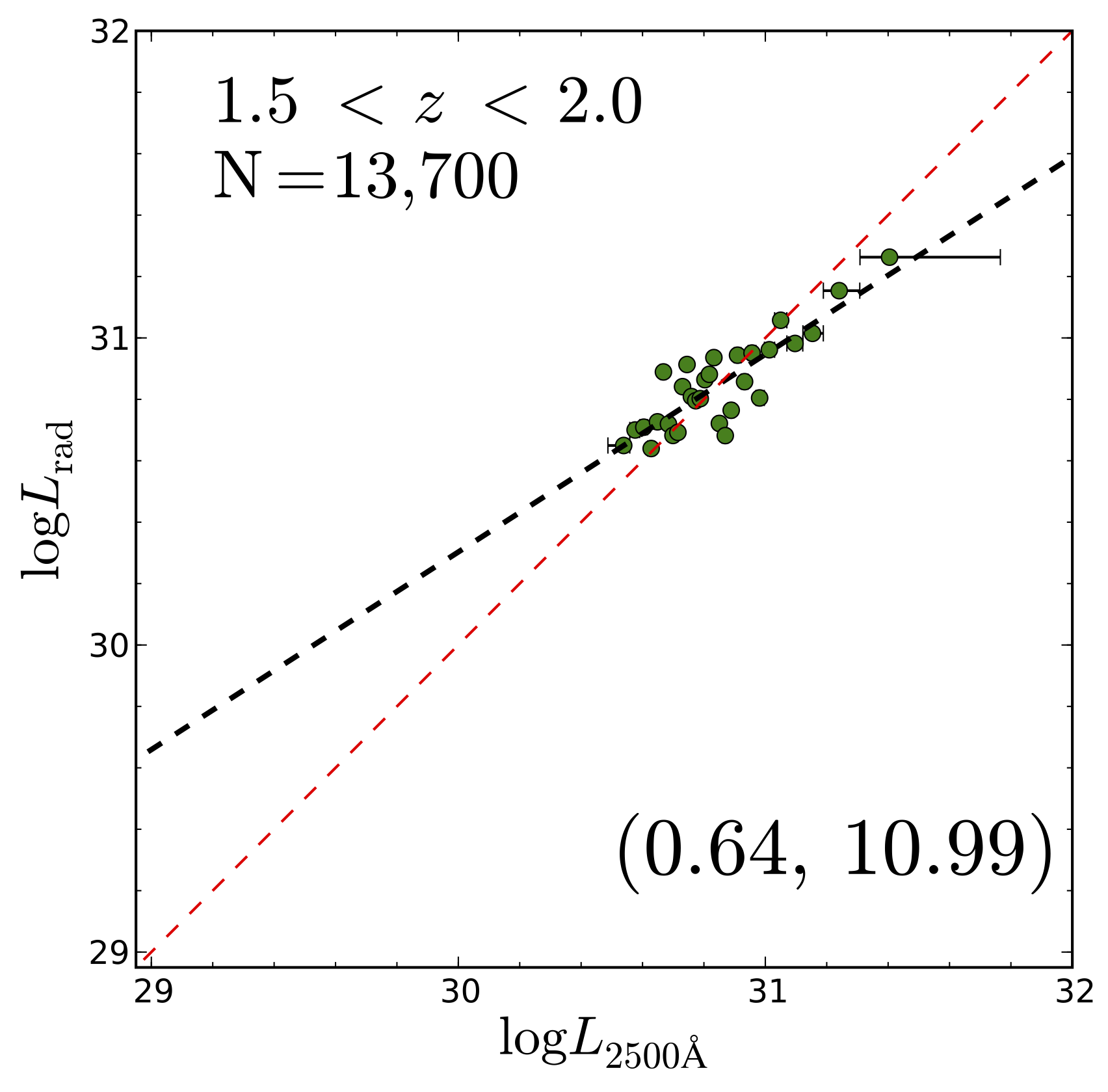
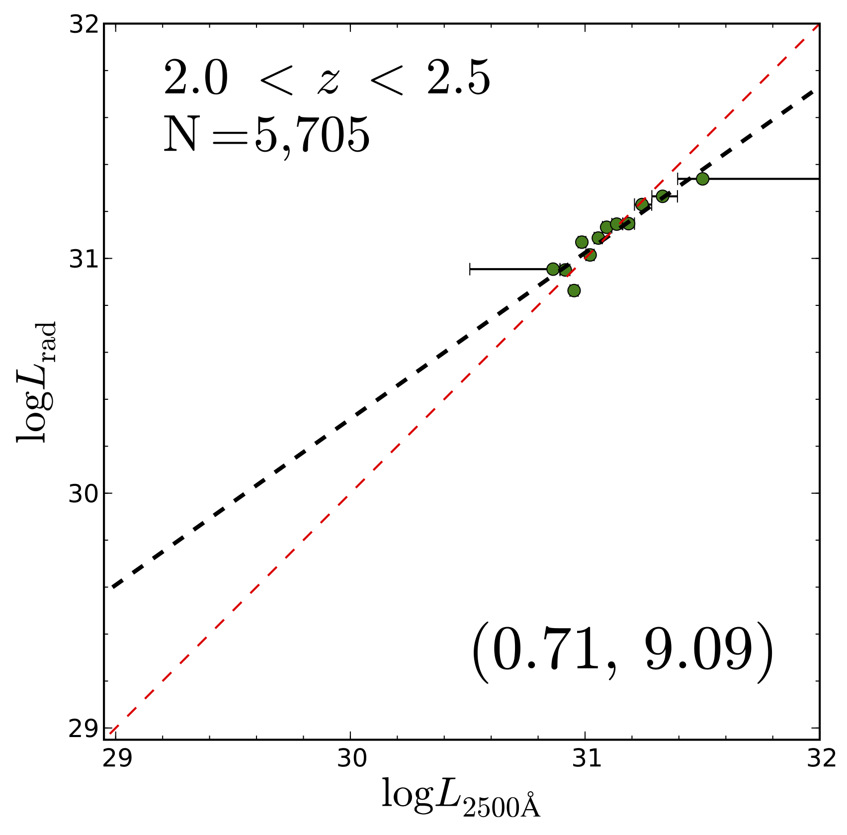
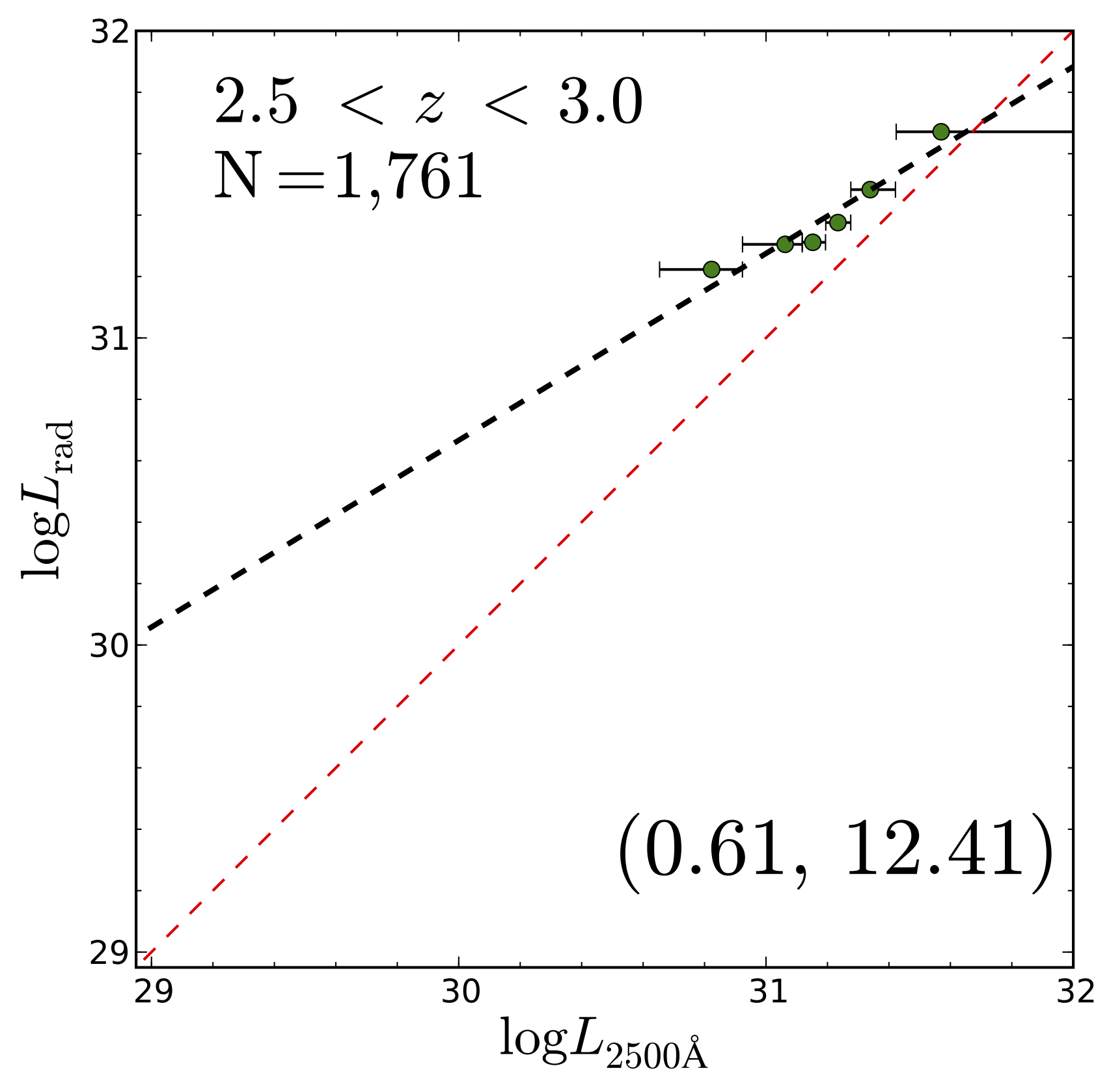
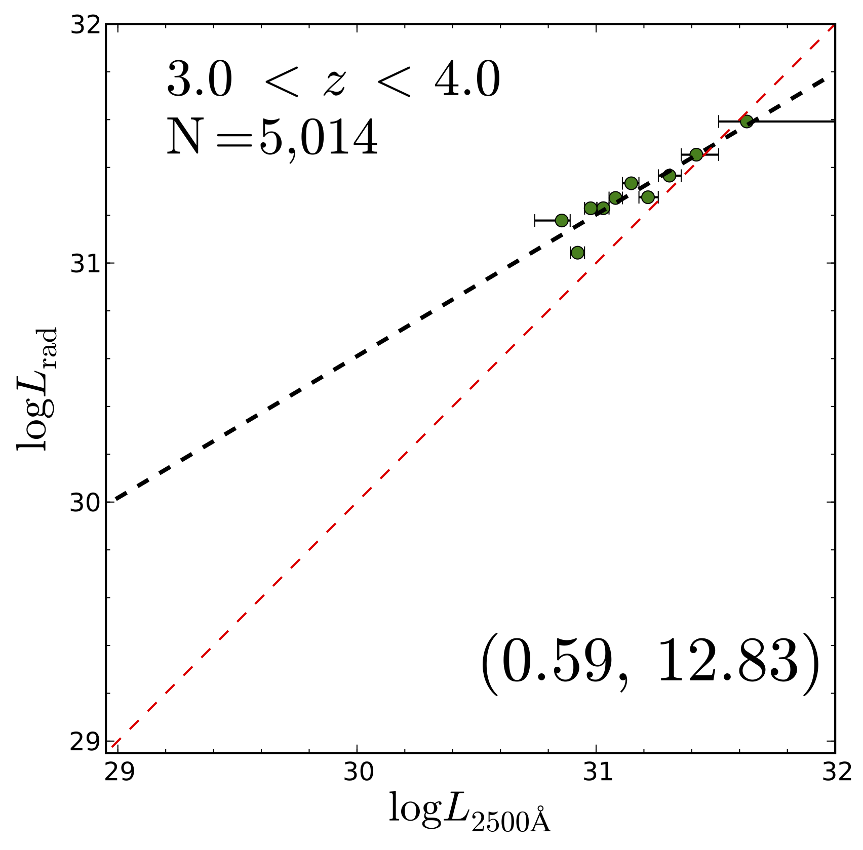
Figure 17: Radio luminosity dependence on $L_{2500\,\rm{\AA}}$ within different redshift intervals (see White et al., 2007, Fig. 10) for Sample B. The dashed red line in each plot shows where $L_{\rm rad}={L_{\rm opt}}$. The best fit lines for each redshift range are shown as the different dashed black lines, and the values in the lower-right corner indicate the slopes and intercepts of these lines. Sample B shows a non-linear relationship between $L_{\rm rad}$ and ${L_{\rm opt}}$, as $L_{\rm rad}\sim{L_{\rm opt}}^{.92}$.

The best fit line is computed as $\log(L_{\rm{rad}})=m\,\log(L_{\rm 2500\,\AA})\,+\,b$, where the median $L_{2500\,\rm{\AA}}$ value for each bin was used and the coordinate pairs $(m,b)$ represent the slope and y-intercept for the linear best fit models. Just as in White et al. (2007), the radio luminosities for our four samples do not increase linearly with the optical luminosities. For low redshift ($z<2.2$) point-source quasars within Sample B, we find that the relationship is $L_{\rm rad}\sim{L_{\rm opt}}^{0.92}$. This corresponds to a factor of $~{}2.5$ in radio luminosity between the least and most luminous quasars in the optical, similar to what was found by White et al. (2007). This deviation from a linear relationship is not as strong as it is in the X-ray (exponent of $\sim 0.72$ in Steffen et al. 2006); however, the lever arm in extrapolating from the optical to the radio is longer than that between the optical and X-ray, and any deviation from linearity is still important to account for.

In Figure 18a, we effectively show the same information as is given in Figure 17, but we have color-coded the different redshift regions and are now plotting $\alpha_{\rm{ro}}\,$ on the $y$-axis. To compute our stacked $\alpha_{\rm{ro}}\,$values, each of the radio cutouts (in Jy) is first divided by its corresponding quasar’s optical flux. Then, the cutout ratios within a bin are median stacked and the maximum pixel value in the stacked image is taken to be $f_{5\,\rm GHz}/f_{\rm 2500\,\AA}$. Finally, the median $\alpha_{\rm{ro}}\,$ value is found by plugging into Equation 4. Here we find that the redshift regions occupy wedge-shaped distributions that are consistent with the flux-limited nature of the quasar sample. As such, our best-fit line (for $z<2$) removes quasars above $\log{L_{2500\,\rm\AA}}=30.75$ beyond which there is an artificial bias in the sample.

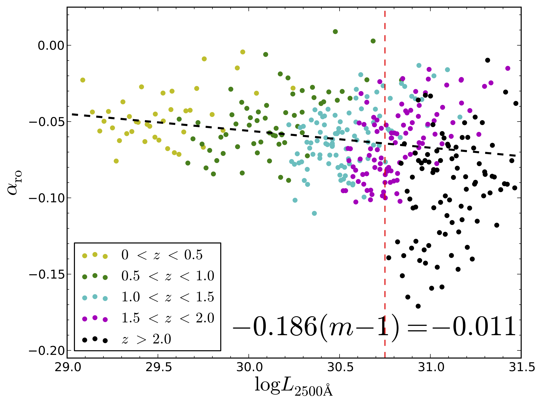
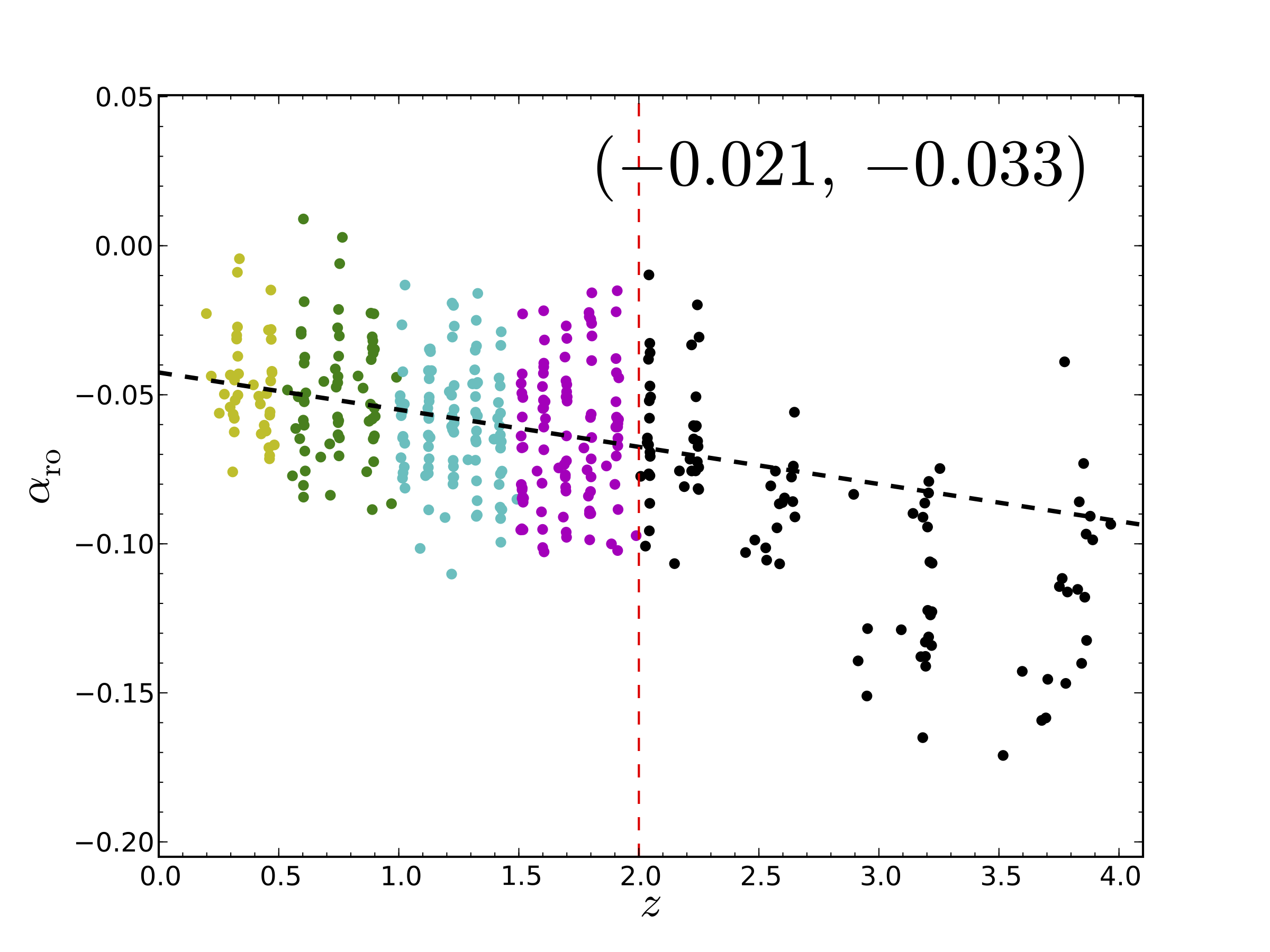
Figure 18: Left: The dependence of $\alpha_{\rm ro}$ on $L_{2500\,\rm{\AA}}$ (see Steffen et al., 2006, Fig. 5, top). The dotted black line is the linear best fit for Sample B. Recall that more negative values of $\alpha_{\rm ro}$ mean more RL; thus, the higher luminosity objects are biased to a more RL SED. Different redshift bins are highlighted with different colors. We have removed sources to the right of the dashed red line when computing the linear best fit so as to not artificially skew it based on selection effects. Right: The dependence of $\alpha_{\rm ro}$ on redshift (see Steffen et al., 2006, Fig. 7, top). The discrete appearance of the points in this panel is an artifact of initially binning our samples with respect to redshift.

The equation reported for the linear best fit model is $\alpha_{\rm ro}=-0.186(m-1)\,\log(L_{\rm 2500\,\AA})\,-0.186\,b$, such that the values of $m$ and $b$ have the same meaning in both Figure 18a and Figure 17. All four of our samples (although only Sample B is pictured) show that $\alpha_{\rm ro}$ decreases (gets more radio-loud) as $L_{2500\,\rm{\AA}}$ increases. This is opposite to what we found in Figure 17 and would seem to be due to the biased nature of the redshift slices in Figure 17 as highlighted by the color-coding of Figure 18a. Indeed, Figure 18a suggests that there is a small increase in radio luminosity with optical luminosity (consistent with $L_{rad}\sim{L_{opt}}^{1.011}$).

Since our samples are flux limited, any evolution in $L$ could instead be an evolution in $z$. As such, we reproduced Figure 18a with redshift instead of $L_{2500\,\rm{\AA}}$ to be sure that there were no additional biases. Figure 18b shows the dependence of $\alpha_{\rm ro}$ on $z$ (see Steffen et al., 2006, Fig. 7, top). The coordinate pair $(a,B)$ represents the slope and y-intercept for the linear best fit model such that $\alpha_{\rm ro}=a\,z\,+\,B$, where we have limited the fitting to data with $z<2.0$ as we did in Figure 18a. All four of our samples (Sample B, pictured) show that $\alpha_{\rm ro}$ slightly decreases with increasing $z$. This trend with redshift is larger than that seen in the X-ray (Steffen et al., 2006).

It is an open question as to whether we should be using $\alpha_{\rm{ro}}\,$ (see Equation 4) or $\Delta\alpha_{\rm{ro}}\,$ $=\alpha_{\rm{ro},\,\rm obs.}\,-\,\alpha_{\rm{ro},\,\rm best\,fit}$ (i.e., $\alpha_{\rm{ro}}\,$ corrected for luminosity and/or redshift) in our analysis. The shape of the SED is measured by $\alpha_{\rm{ro}}\,$ whether or not $\alpha_{\rm{ro}}\,$ has any luminosity or redshift dependences. If it is the shape that matters (as it is for the dependence of radiation line-driven winds on $\alpha_{\rm{ox}}\,$), then we should be using $\alpha_{\rm{ro}}\,$. In that case, our current analysis will suffice. If, on the other hand, we care more about the shape relative to the mean at a given $L$ or $z$, then we should be using $\Delta\alpha_{\rm{ro}}\,$. For example, if dust reddening were causing a trend in $\alpha_{\rm{ro}}\,$ with $L$, we might prefer to use $\Delta\alpha_{\rm{ro}}\,$. Indeed, absorption is an issue for $\alpha_{\rm{ox}}\,$; however, in our case, the relative deficit of optical flux is for the most luminous sources, not the least luminous. Therefore, it is unlikely that dust reddening is causing the increase in radio-loudness with luminosity.

We can see this in another way in Figure 19 which shows the mean relative color in each of the bins. Ignoring the lowest redshift quasars (where host galaxy contamination makes determining the relative colors difficult), we see that there is no strong trend towards redder colors with fainter magnitudes. As such, it would appear that dust is not the explanation the cause of the trend of $\alpha_{\rm{ro}}\,$ in $L-z$ space.

A more accurate determination of the $L$ and $z$ dependence of $\alpha_{\rm{ro}}\,$ is a question suitable for its own investigation (e.g., Steffen et al. 2006). We will leave our analysis in terms of $\alpha_{\rm{ro}}\,$, noting that the trends could change with $\Delta\alpha_{\rm{ro}}\,$.

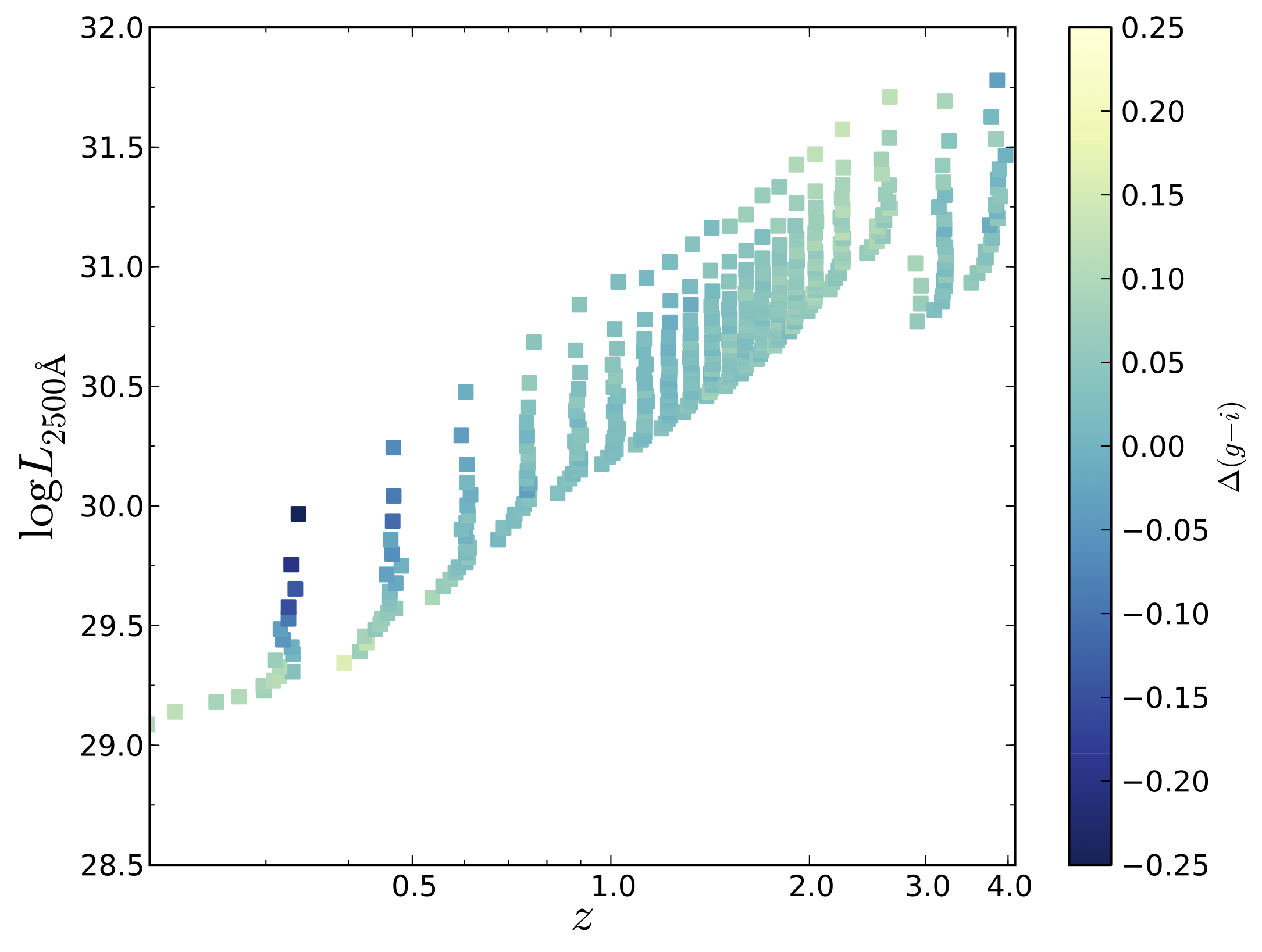
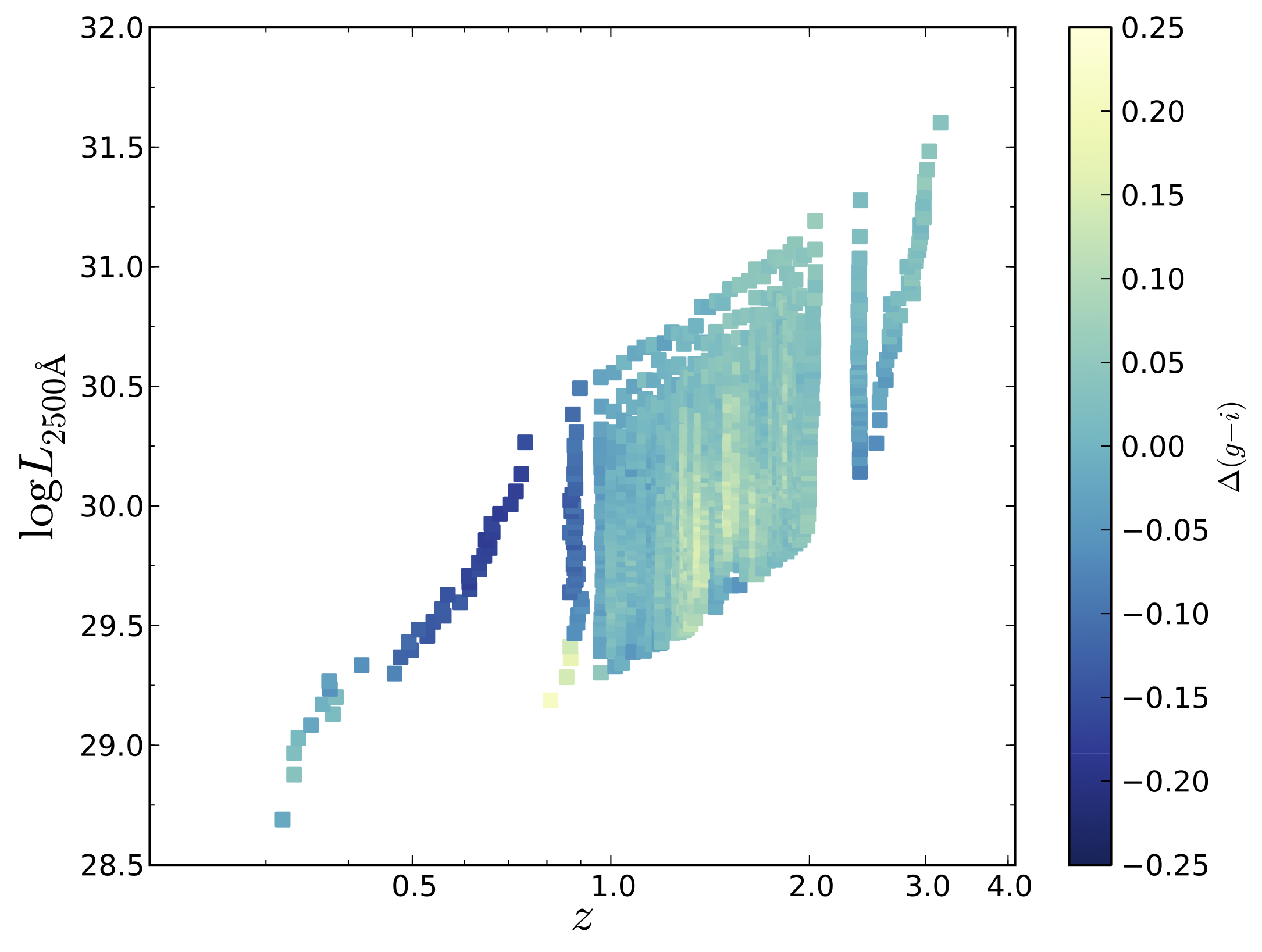
Figure 19: The relative color, $\Delta(g-i)$, of median stacked quasars as a function of both redshift and $L_{2500\,\rm{\AA}}$. These bins are the same as those used in Figures 14, 15, and 16. The distribution of $\Delta(g-i)$ values in the $L-z$ plane shown suggest that dust is not the cause of the trends in mean radio loudness with $L$ and $z$.

4 Results

4.1 The $L$ and $z$ Distributions

We begin our comparison of mean and extreme radio properties of quasars in the $L-z$ parameter space. Figure 20 (left) shows how the RLF of equally populated bins depends on both redshift and $L_{2500\,\rm{\AA}}$ for Sample B. We find that the RLF declines with increasing redshift (for a given luminosity) and decreasing luminosity (for a given redshift). These results would appear to confirm the findings of Jiang et al. (2007) by using at least twice the number of sources.

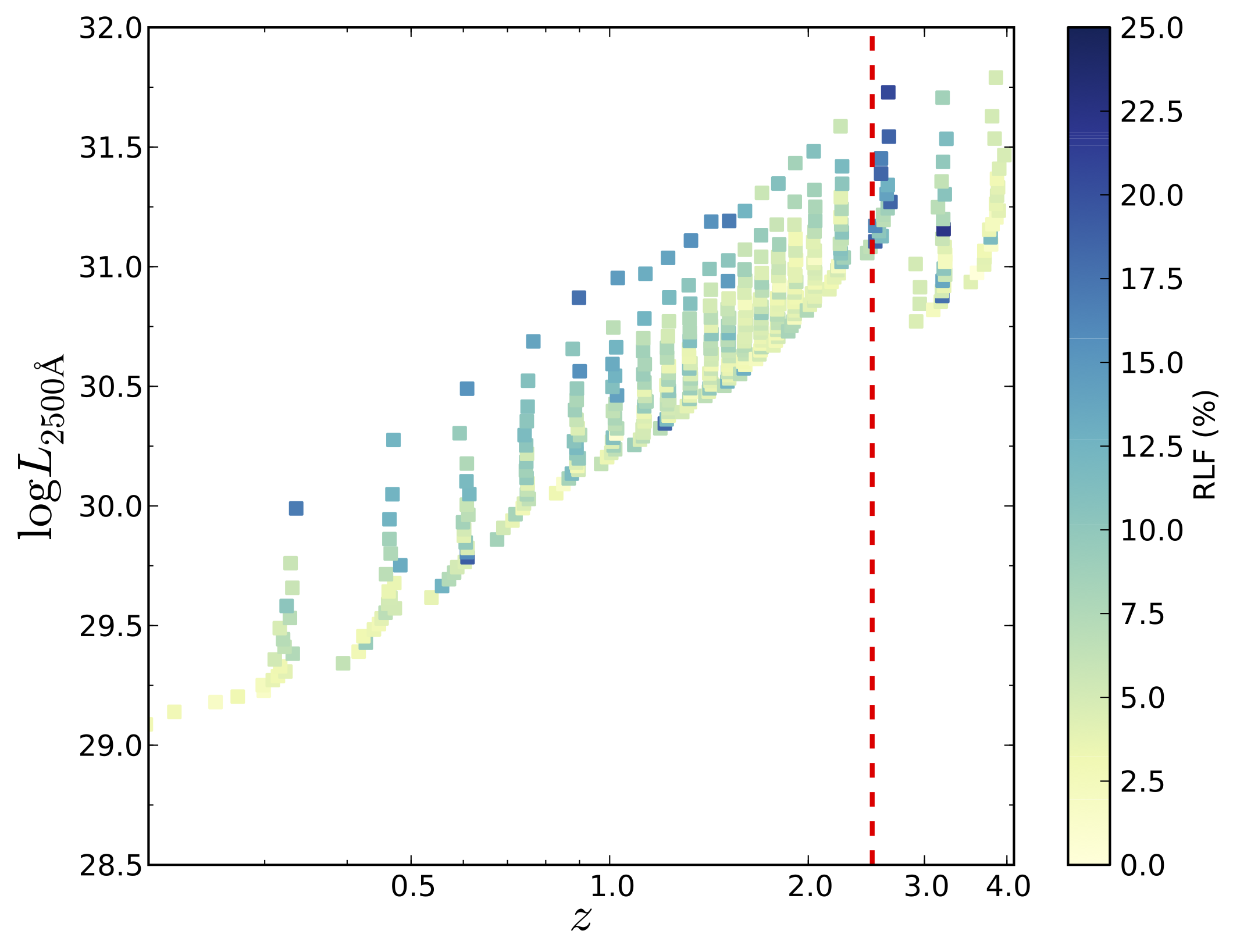
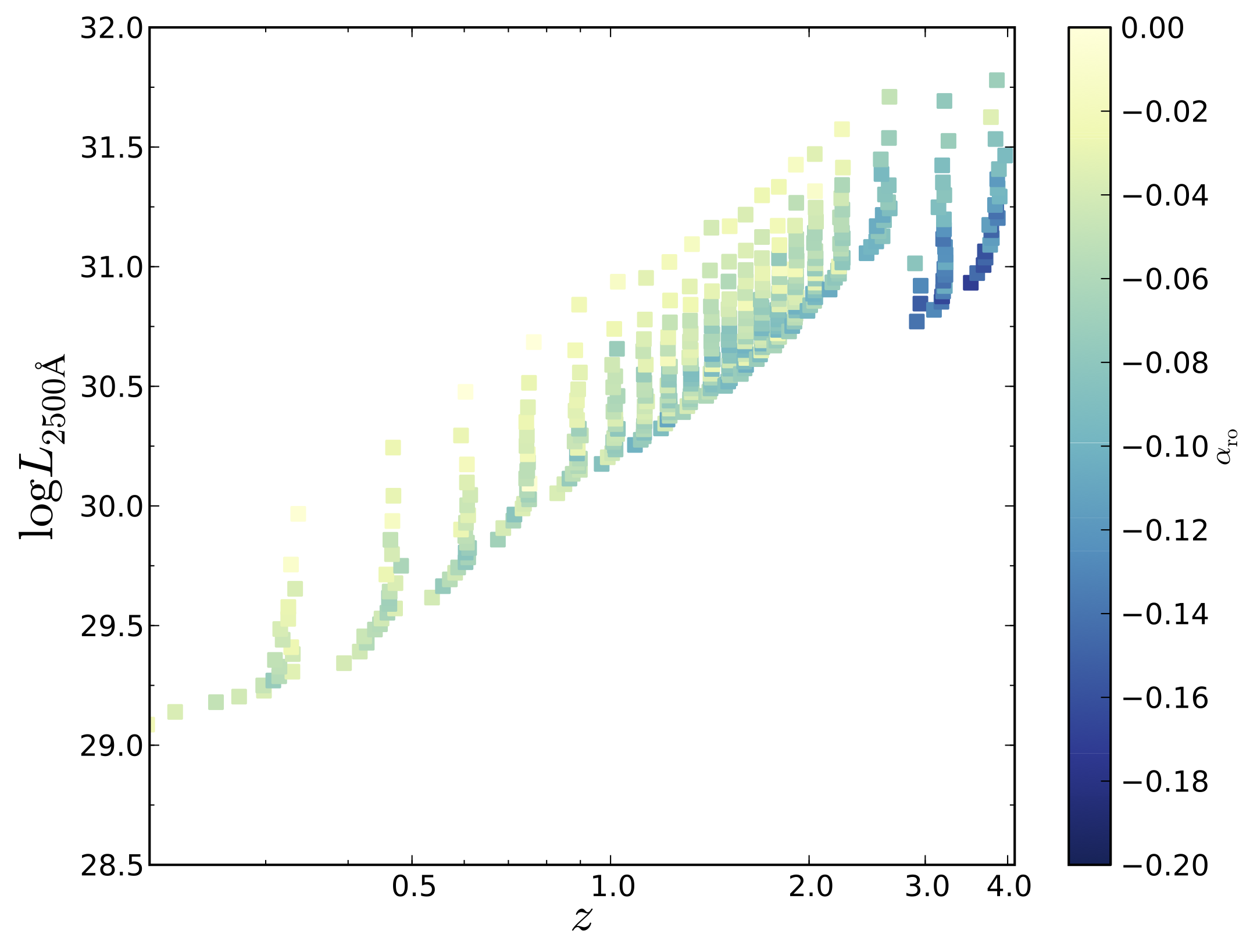
Figure 20: (Left:) RLF as a function of both $L_{2500\,\rm{\AA}}$ and redshift for optically detected quasars within the FIRST observing area for Sample B. The RL completeness correction (see Section 2.6.5) has been applied. The boundary on the lower edge represents the SDSS flux limit of $i<19.1$ for $z<3$ and $i<20.1$ for $z>3$. The trend seen confirms the results of Jiang et al. (2007) by demonstrating a decrease in RLF with increasing redshift and decreasing luminosity. (Right:) Radio to optical spectral indices ($\alpha_{\rm ro}$) of median stacked quasars as a function of both redshift and $L_{2500\,\rm{\AA}}$. This trend is completely opposite to that found for the RLF in the left panel. The median stacking shows stronger radio sources (relative to the optical) with decreasing optical luminosity (at fixed redshift) and with increasing redshift (at fixed optical luminosity).

Contrasting the RLF trend in the left-hand panel of Figure 20 is the $\alpha_{\rm{ro}}\,$ trend in the right-hand panel. Specifically, we find that quasars are stronger radio sources (relative to the optical) with decreasing optical luminosity (at fixed redshift) and with increasing redshift (at fixed optical luminosity). Thus, it appears that the mean radio properties of quasars are not following the same trends as the extreme RL population. Singal et al. (2011) similarly find increasing radio loudness with increasing redshift. Their apparent discrepancy with the results of Jiang et al. (2007) can be explained by the difference between the mean radio-loudness (as is shown in Figure 20 [right] and in Singal et al. 2011) and the RLF (as is shown in Figure 20 [left] and in Jiang et al. 2007). Our results are consistent with both papers when considered in this light. Thus, for these two parameters, the mean radio properties of quasars are not following the same trends as the extreme RL population. Indeed, Baloković et al. (2012) also find that, as redshift increases, quasars become both more RL on average but also less likely to inhabit the formally RL tail of the distribution.

We note that the trends in Figure 20 are such that the RLF declines (and the mean radio loudness increases) in the direction following decreasing $i$-band magnitude (see also Jiang et al. 2007, Figure 7a and Baloković et al. 2012, Figure 10). As it is not clear why an intrinsic quasar property should be a strong function of the apparent magnitude, these results must be taken with a grain of salt. As noted in Section 2.6.5, the completeness correction should be good down to a radio flux of $\sim$2.5 mJy. However, plugging that value into Equation 5 of Ivezić et al. (2002), we find that our analysis is only robust to $i=17.9$ which is not deep enough to determine if the separate RLF trends in $L_{2500\,\rm{\AA}}$ and $z$ are real or due to incompleteness (or some other selection effect). Thus, for the case of the RLF, there must be concern that incompleteness could be causing that dependence. A radio survey covering a significant fraction of the FIRST area and to at least 3$\times$ the depth of FIRST would be needed to test this effect. However, our stacking analysis should be independent of the completeness of FIRST, which argues that the $\alpha_{\rm{ro}}\,$ trend with optical magnitude may be real.

Another issue with this type of analysis is that if the radio distribution does indeed require two components (or if it is bimodal), then it may be the case that the dividing line between the populations should change with luminosity as noted by Laor (2003). Thus, it is possible that we could be under- (or over-) stating the trends with RLF in Figure 20. As we cannot establish to what extent these trends are robust, we move on to looking for other demographics to provide further constraints on the nature of radio-loud emission in quasars. We will discuss the interpretation of Figure 20 further in Section 5.

4.2 Accretion Disk Winds: Principal Component and CIV Analyses

As noted by White et al. (2007), the problem is essentially that there is no practical way to identify from optical properties of quasars which individual quasars are likely to be radio-loud. We hope that extending our analysis to more detailed spectral properties of quasars in the optical/UV will offer more insight. Arguably the most in-depth analysis of quasar spectral properties has come from the Principal Component Analysis (PCA) first carried out by Boroson & Green (1992).

Boroson & Green (1992) showed that significant new insight could be gained by examining the range of differences in quasar continua and emission lines using a PCA (or “eigenvector”) analysis. They found that the properties of the H$\beta$, O III], and Fe II emission lines were well correlated with other differences seen in quasar spectra. Moreover, they found that these differences were correlated with the radio continuum in a way that suggested that RL and RQ quasars are not “parallel sequences” due to a lack of RQs matching the extremes of the RL sample. Boroson (2002) extended this work with a larger sample and Brotherton & Francis (1999) and Sulentic et al. (2000a) added additional line and continuum features to this matrix of quasar “eigenvectors”.

Sulentic et al. (2000b) showed that much of the information from the first eigenvector of quasar properties is captured by simply looking at the FWHM of H$\beta$ and the strength of optical Fe II emission relative to H$\beta$, R${}_{\rm Fe\,II}$ = W(Fe II $\lambda$4570 blend)/W(H$\beta_{\rm BC}$). They used this diagram to divide quasars into two populations (A/B). While there is a continuum between the populations, it is useful to think of the extrema in this context, and they found that RL quasars are generally isolated to Population B, whereas RQ quasars appear in both; see also Zamfir et al. 2008.

In that context, we consider the radio properties of the quasars in our samples in this simplified “Eigenvector 1 (EV1)” parameter space. The left panel of Figure 21 shows how the RLF of equally populated bins evolves in low-redshift EV1 parameter space (FWHM H$\beta$ vs. R${}_{\rm Fe\,II}$) for all samples, while the right panel gives the median $\alpha_{\rm{ro}}\,$ values. The highest RLFs are found in the top-left (typically hard spectrum) corner of each panel, consistent with the findings of Sulentic et al. (2000b). Importantly, there is no gradient in optical magnitude in this parameter space, so this result must be more fundamental than our analysis of the $L-z$ distribution, which was subject to vagaries of FIRST completeness corrections.

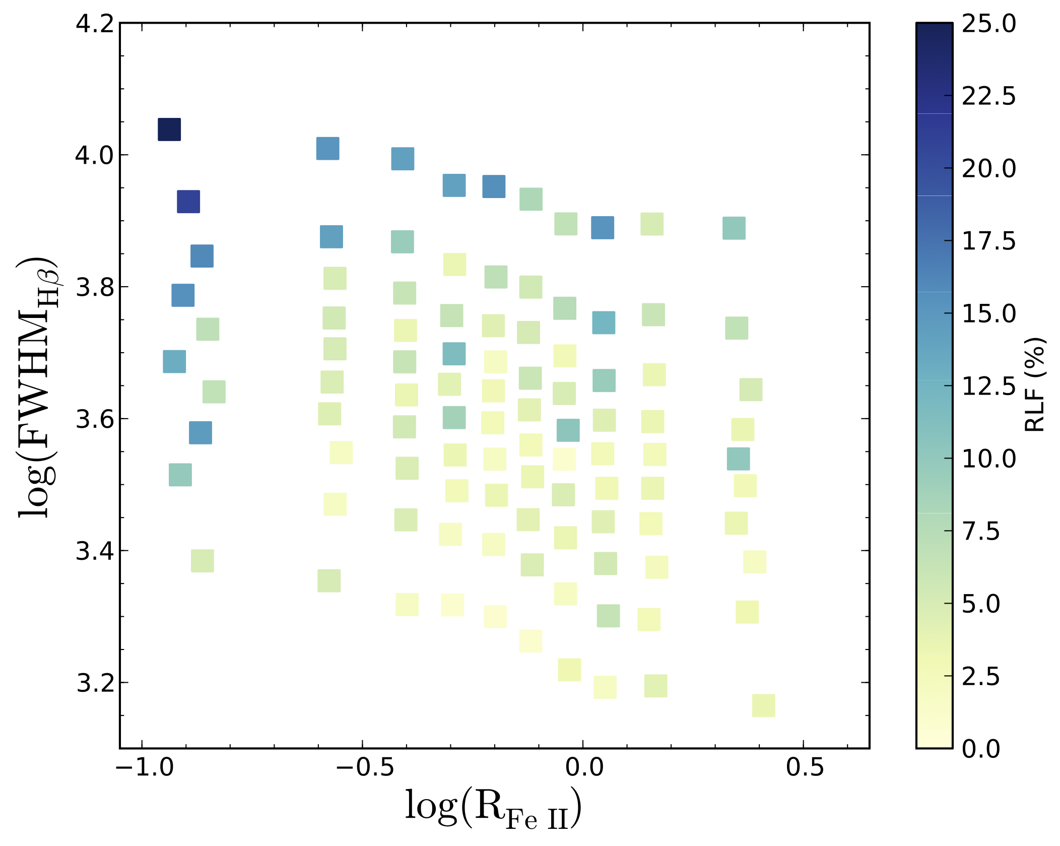
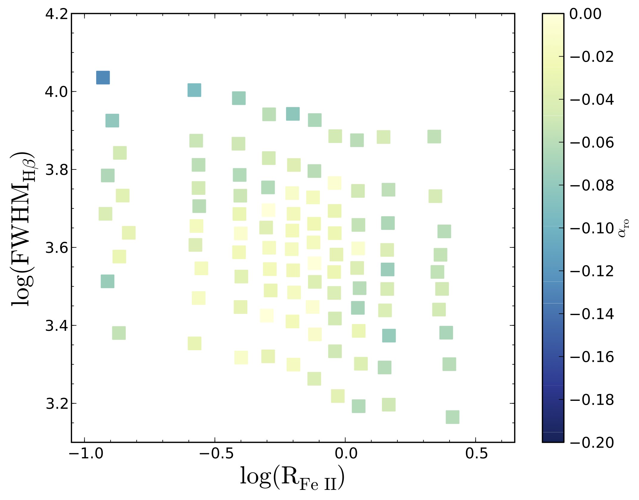
Figure 21: Radio properties of quasars in the low-$z$ EV1 (FWHM H$\beta$ vs. R${}_{\rm Fe\,\rm II}$) parameter space for optically detected quasars within the FIRST observing area. (Left:) The RLF, where the RL completeness correction (see Section 3) has been applied. The highest RLF bins are concentrated to the high FWHM H$\beta$-low R${}_{\rm Fe\,II}$ corner of this low-$z$ EV1 parameter space (in agreement with Sulentic et al. 2000b). (Right:) Radio to optical spectral indices ($\alpha_{\rm ro}$) of stacked quasar cutouts in low-$z$ EV1 parameter space. Here there is not as clear a trend, but the bin with the most radio-loud sources also has the largest H$\beta$ FWHM and the weakest Fe II.

There is less of a discernible trend in the mean radio properties as shown in the right-hand panel of Figure 21 than for the RLF in the left-hand panel. However, we note that the most RL sources (most negative $\alpha_{\rm{ro}}\,$) are still those in the top-left corners with the broadest H$\beta$ and weakest Fe II emission lines.

While EV1 encodes the largest differences in otherwise similar quasar spectra, the objects which this type of analysis is based upon are necessarily low-redshift (as the spectrum must cover H$\beta$). However, the mean SDSS quasar has a redshift closer to $z\sim 1.5$, where the EV1 parameters are no longer included in the optical. To this end, it has been shown that the C IV emission line can be used to isolate extrema in quasar properties at high-redshift in a manner similar to EV1 at low-redshift (e.g., Sulentic et al., 2000a; Richards et al., 2002a; Sulentic et al., 2007; Richards et al., 2011). It would appear that high-redshift quasars occupy a broader parameter space than low-redshift quasars, presumably due to a larger diversity of black hole masses and accretion rates. Richards et al. (2011) argue that this diversity can be connected to the ability of a quasar (through its intrinsic SED) to power a strong radiation line-driven wind and that the C IV line represents an EV1-like diagnostic.

Specifically, Richards et al. (2011) argue that the C IV emission line properties of a quasar, particularly the equivalent width (EQW) and the “blueshift” (the offset of the measured rest-frame line peak from the expected laboratory value), can provide an understanding of the trade-off between the disk and wind parameters of quasars (see Murray et al., 1995; Elvis, 2000; Proga et al., 2000; Leighly, 2004; Casebeer et al., 2006; Leighly et al., 2007). The C IV emission line is a good diagnostic for a variety of reasons. Aside from Ly$\alpha$, it is the most conspicuous emission line in high-redshift quasars, which allows for high S/N measurements of this line in many objects. More importantly, the EQW and blueshift of C IV have the largest range of emission line properties for all high redshift quasars, increasing our ability to locate trends. Additionally, the blueshifting of the C IV line with respect to the quasar’s rest frame (Gaskell, 1982; Wilkes, 1984) is practically universally present in spectra of luminous quasars (Sulentic et al., 2000b; Richards et al., 2002a).

In the context of a C IV analysis, Richards et al. (2011) find that RQ quasars span the full space occupied by both quasar types—in contrast to findings of Boroson & Green (1992) and Boroson (2002). On the other hand, the RL quasars were largely confined to that part of parameter space with small C IV blueshifts (and large EQWs) (see Richards et al., 2011, Fig. 7). Richards et al. (2011) interpret this result in a disk-wind framework and argue that, on average, RL quasars have weaker radiation line-driven winds than RQs.

Here we take the analysis of the radio properties of quasars in C IV parameter space one step further than Sulentic et al. (2007) and Richards et al. (2011). Specifically, we have repeated our dual analyses in C IV parameter space. Figure 22 (left) shows that the RLF primarily decreases from low to high blueshift. No discernible RLF trend exists with respect to EQW. In terms of the mean radio properties shown in the right-hand panel of Figure 22, the mean trend is in the same general direction as the RLF trend, but is weaker—similar to the EV1 trends in Figure 21. However, it does appear that small-blueshift quasars are more radio loud, on average, than those with large C IV blueshifts.

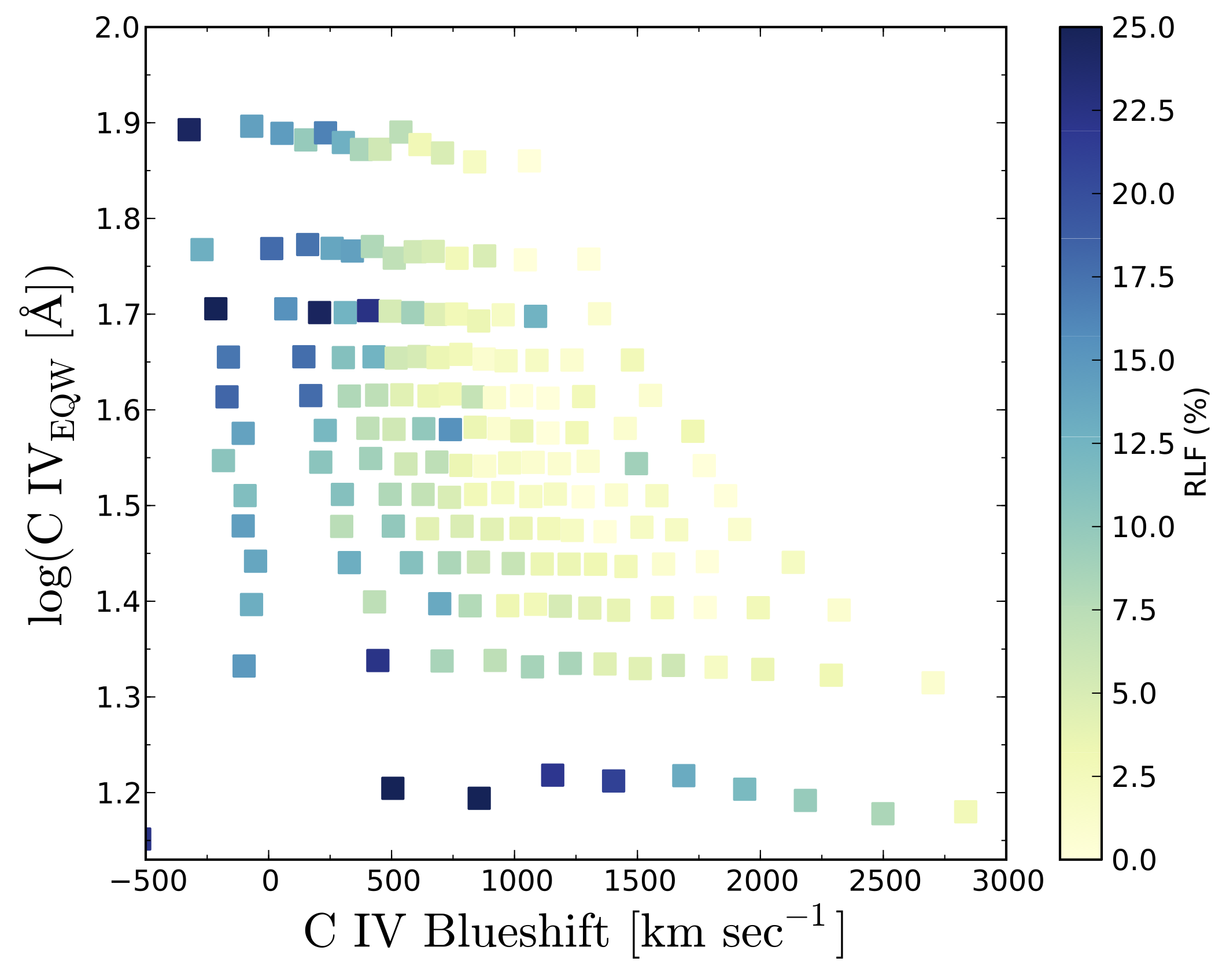
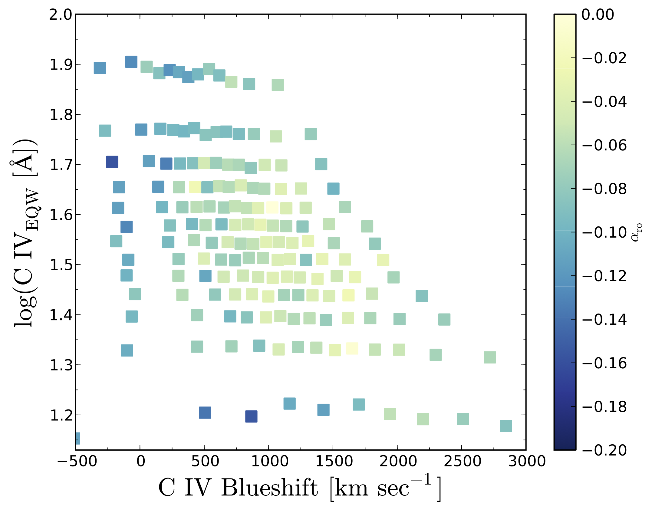
Figure 22: Radio properties as a function of both C IV equivalent width (EQW) and blueshift for optically detected quasars within the FIRST observing area. (Left:) The RLF, including the RL completeness correction (see Section 3). The RLF primarily decreases from low to high blueshift with no discernible RLF trend in EQW; see also Richards et al. (2011). Objects in the row with the lowest EQWs likely have higher RLFs due to selection effects. (Right:) Radio to optical spectral indices ($\alpha_{\rm ro}$) of stacked quasar cutouts in C IV parameter space. As with the EV1 parameter space, the mean shows a weaker trend than the RLF that evolves in the same direction.

Ideally our goal here is to be able to identify a UV emission line parameter that would predict whether or not an individual quasar is radio-loud. Although we have not accomplished that goal, we can use this analysis to improve the statistical prediction from a blanket $\sim 10$% to a fraction that ranges from $\sim$0% to $\sim$30% as a function of C IV emission line properties. In one sense this does allow a prediction of radio properties for at least some quasars as it seems that quasars at the extreme end of the C IV blueshift distribution (for a given C IV EQW) are exceedingly unlikely to be radio-loud.

4.3 Black Hole Mass and Accretion Rate

Two of the most important properties that govern how quasars behave are the mass of the central black hole (BH) and its accretion rate. While we cannot measure the mass and accretion rate of a black hole directly, we can derive estimates of these values by using so-called BH mass scaling relations (e.g., Vestergaard & Peterson, 2006) in conjunction with emission line and continuum information. We now explore how the RLF behaves as a function of these BH mass estimates.

BH masses were compiled by Shen et al. (2011) and have been corrected as described in Section 2.3. Assuming a bolometric correction of $L_{\rm Bol}=2.75L_{\rm 2500\,\AA}$ (Krawczyk et al., 2013), we can convert $L_{2500\,\rm{\AA}}$ to $L_{\rm Bol}$ to determine the Eddington Ratio, $L_{\rm Bol}/L_{\rm Edd}$, where $L_{\rm Edd}$ is derived directly from the BH mass estimate. Figure 23 shows how the radio-loud fraction (of equally populated bins) depends on $L_{2500\,\rm{\AA}}$ (effectively accretion rate) and black hole mass. We have presented the data in this way instead of plotting $L/L_{\rm Edd}$ directly; Richards et al. (2011) argue that it is optimal to investigate BH mass and accretion rate separately in case there are any threshold effects (low mass/low accretion rate can have the same $L/L_{\rm Edd}$ as high mass/high accretion rate, but potentially very different properties). Nevertheless, $L/L_{\rm Edd}$ appears as dashed red lines in Figure 23. The line on the lower-right indicates $L/L_{\rm Edd}=1$, or (theoretical) maximal accretion (per mass), while the line on the top left is at $L/L_{\rm Edd}=0.01$ and the line in the middle represents $L/L_{\rm Edd}=0.1$.

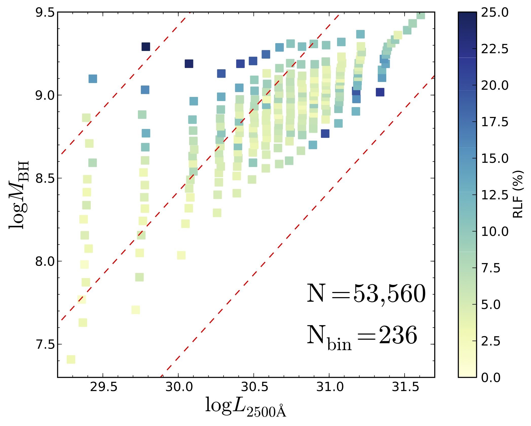
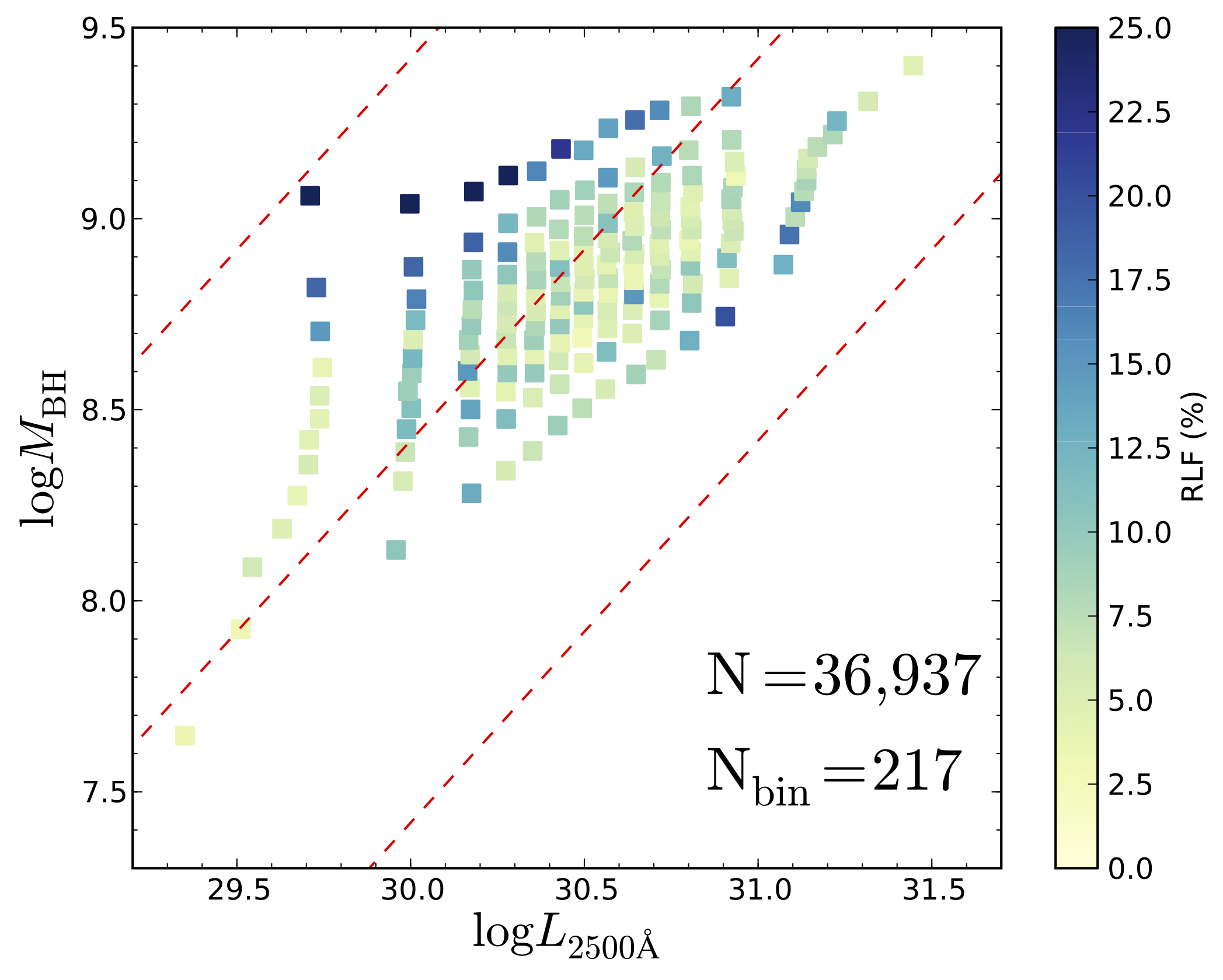
Figure 23: RLF as a function of BH mass and accretion rate for quasars within the FIRST observing area for Samples B (left) and D (right). As with all of our RLF plots, we have corrected for RL completeness (see Section 2.6.5). For both samples, the highest RLFs are positioned in the corners of parameter space: high BH mass for the lowest accretion rates and low BH mass for the highest accretion rates. The dashed red lines show where $L/L_{\rm Edd}=0.01$, $0.1$, and $1.0$ in order from top-left to bottom right. We assume $L_{\rm Bol}=2.75L_{\rm 2500\,\AA}$ (Krawczyk et al., 2013).

In Figure 23, we find that the bins with the highest RLFs are situated in the corners of parameter space, specifically high BH mass/lowest accretion rate and low BH mass/highest accretion rate. The lowest RLFs exist in a diagonal band that stretches from low BH mass for the lowest accretion rates to high BH mass for the highest accretion rates.

Since the estimation of BH masses in high-redshift quasars by way of scaling relations is not an exact science and is dependent on the emission lines used, we also create subsamples based on the origin of these masses (see Figure 24). Specifically, our sample includes quasars whose masses are estimated using the H$\beta$, Mg II, and C IV emission lines; this roughly corresponds to $z<0.7$, $0.7\leq z<1.9$, and $z\geq 1.9$, respectively. The mass estimates computed using the H$\beta$ and Mg II emission lines are thought to be reliable, shown to be within a factor of 2.5 of the masses found using reverberation mapping (McLure & Jarvis, 2002). Indeed, for the two low-redshift bins we see behavior that is consistent with what we might expect from past work. Namely, that the quasars with the highest masses (at a given luminosity) are the most likely to be radio-loud, though not exclusively radio-loud; most quasars in the RL regions are still RQ (see Lacy et al., 2001).

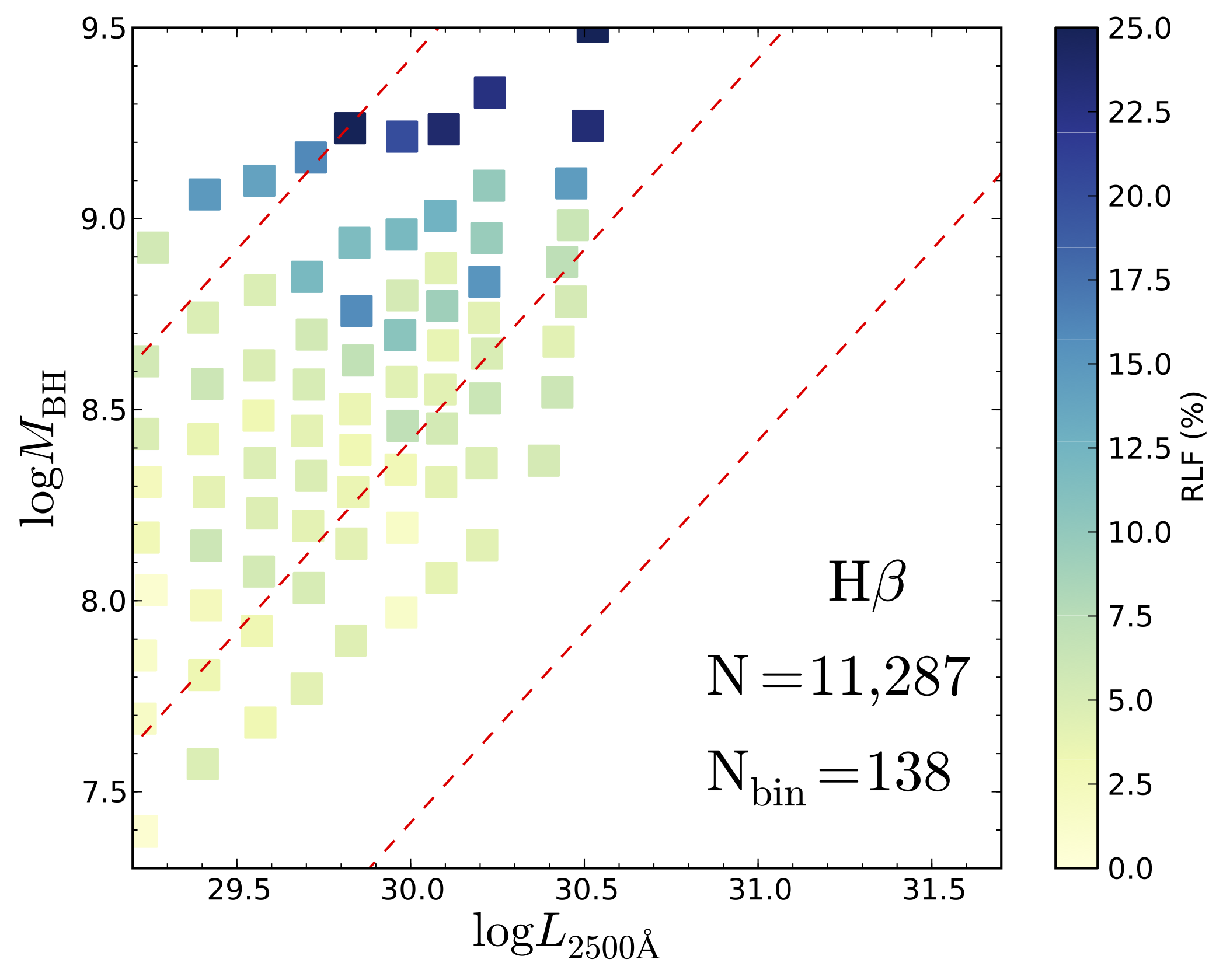
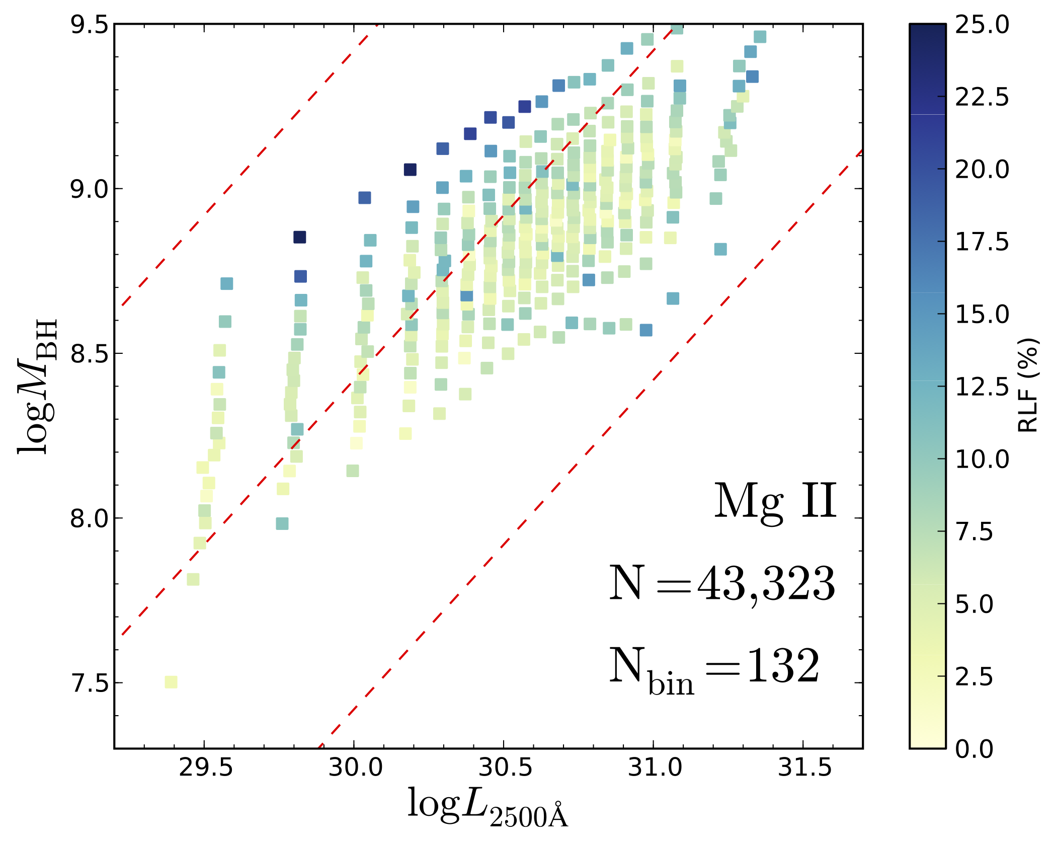
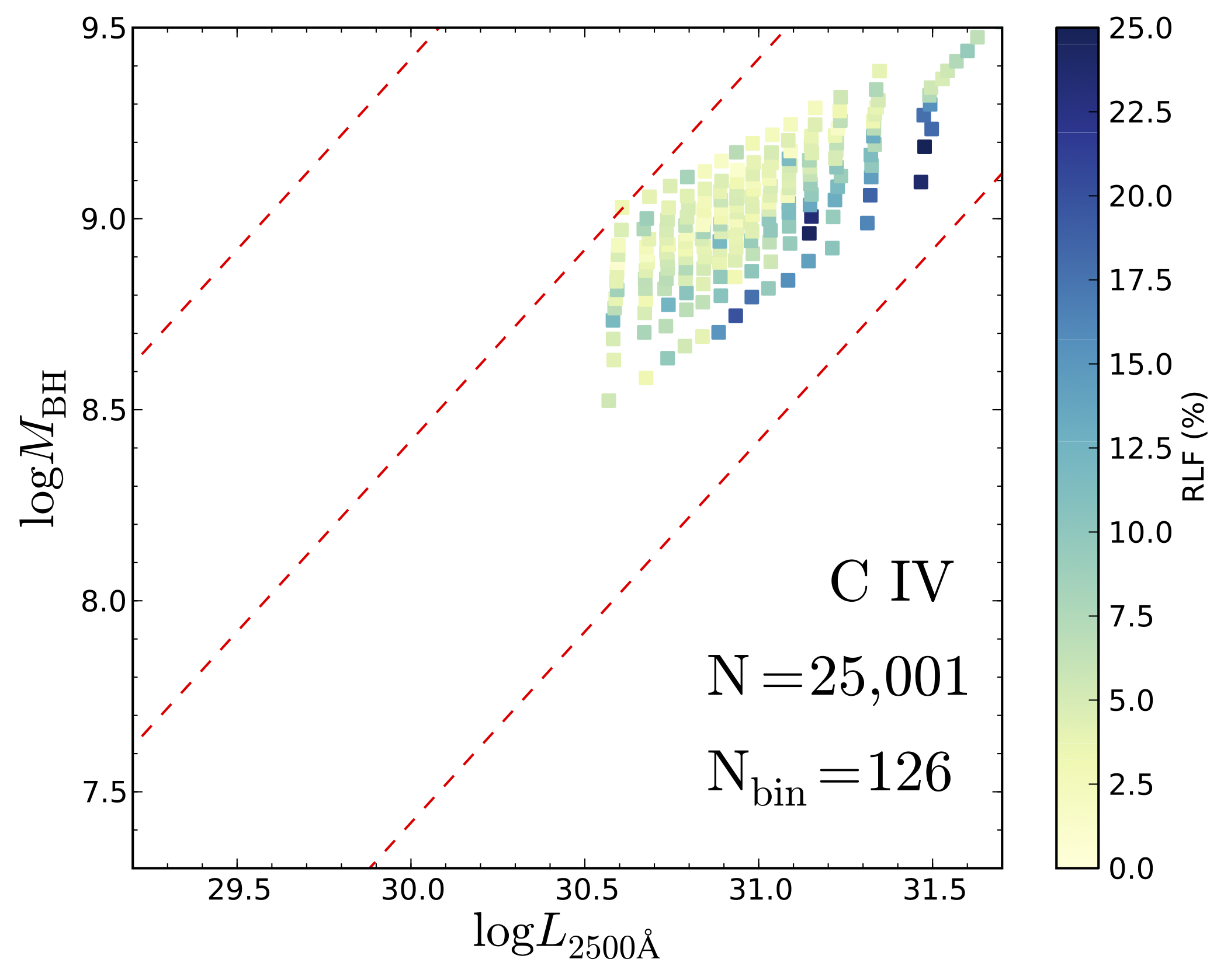
Figure 24: Figure 23, Sample B, split into different populations based on the spectral line used to calculate the BH masses. Each panel effectively represents quasars within different redshift bins (see Shen et al., 2011, Sec. 3.7). For the two lowest redshift samples (H$\beta$ and Mg II), the highest RLFs belong to the highest BH mass bins for these samples. The lowest BH mass bins in the highest redshift sample (C IV) are (apparently) the most RL. We suggest that this difference is indicative of errors in the C IV BH mass estimates. The dashed red lines from top-left to bottom right show where $L/L_{\rm Edd}=0.01$, $0.1$, and $1$, in order. We assume $L_{\rm Bol}=2.75L_{\rm 2500\,\AA}$ (Krawczyk et al., 2013).

However, when we examine the high-redshift subsample, we see something quite different. Here the lowest mass quasars appear to be the most radio-loud. There are a number of potential explanations for this observation. One possibility is that there is an actual physical transition at high redshift such that we are more likely to find RL quasars in high $L/L_{\rm Edd}$ systems. This could be magnified (or perhaps caused) by a change in the selection of quasars from UV-excess sources at $z\lesssim 2$ to $u$-band dropouts at higher redshifts. Alternatively, instead of a physical change, perhaps the high-redshift quasar sample is simply biased against RL quasars with high-mass (at high redshift)? However, we consider this unlikely: although the completeness of FIRST drops with redshift, radio sources are explicitly targeted for spectroscopy as quasars candidates in the SDSS surveys. While there are known incompletenesses in the quasar selection at high-$z$, the most glaring of these has to do with the presence (or lack thereof) of Lyman-limit absorption systems (Worseck & Prochaska, 2011) and is independent of the radio properties of the quasars. Indeed, estimates of the completeness of the SDSS quasar survey (e.g., Vanden Berk et al., 2005) are inconsistent with the extreme level of incompleteness that would be required to induce this effect.

Instead we argue that the problem lies in the estimation of BH masses using the C IV emission line. This could arise from more of the C IV line being emitted in a wind component than has previously been thought or in the form of a wind-strength dependence to the proportionality constant in the radius-luminosity relation (Richards et al., 2011). While it is well-known that determining BH mass scaling relations from the C IV lines are the most challenging (e.g., Fine et al., 2010; Shen et al., 2011; Assef et al., 2011; Denney, 2012; Runnoe et al., 2013; Park et al., 2013; Denney et al., 2013), the corrections necessary for the radio-loudness trend to match the low-redshift BH mass trends are not consistent with the level of “tweaks” to the C IV BH mass scaling relations that are generally advocated. Rather, these BH mass estimates must be catastrophically wrong. Otherwise, these trends would suggest an unlikely situation whereby high-redshift and low-redshift quasars have their radio properties governed by two different process, where the switch just happens to occur at redshifts where the BH mass estimates transition from using Mg II to using C IV. Specifically, high-redshift RL quasars would have to have high $L/L_{\rm{Edd}}$, while low-redshift RL quasars have low $L/L_{\rm{Edd}}$ (c.f. Shankar et al., 2010). Thus this issue is not just a matter for our analysis but speaks to the broader problem of the use of BH masses estimated from C IV emission lines.

To reconcile the low-redshift and high-redshift quasars, the RL quasar masses at high-$z$ are too low by as much 0.5 dex or more and not simply by $\sim 0.2$–0.3 dex as is usually assumed. Technically this statement applies only to the RL quasars. However, as Richards et al. (2011) argue that there are negligible differences in the emission line properties of RL and RQ quasars with small C IV blueshifts, it must also be true that a large fraction of the masses computed for RQ quasars are similarly erroneous. Indeed, it would seem that the C IV BH mass estimates are close to being inverted (large BH mass should be small, and vice versa). As there is only a weak correlation between the BH masses estimated from C IV and Mg II in Shen et al. (2011, Fig. 10), this is perhaps not surprising. We will consider this issue further in Section 5.

We now consider the mean radio-loudness as a function of mass, accretion rate, and $L/L_{\rm{Edd}}$ as we did in Figure 23, plotting just the results for H$\beta$ and Mg II. Specifically, Figure 25 shows mass vs. luminosity color-coded by $\alpha_{\rm{ro}}\,$. For H$\beta$, we find strong similarities between this analysis and the RLF analysis with the most radio loud objects being towards the top left of each panel such that the mean radio-loudness increases towards lower $L/L_{\rm{Edd}}$, consistent with the RLF. There is no obvious trend for Mg II.

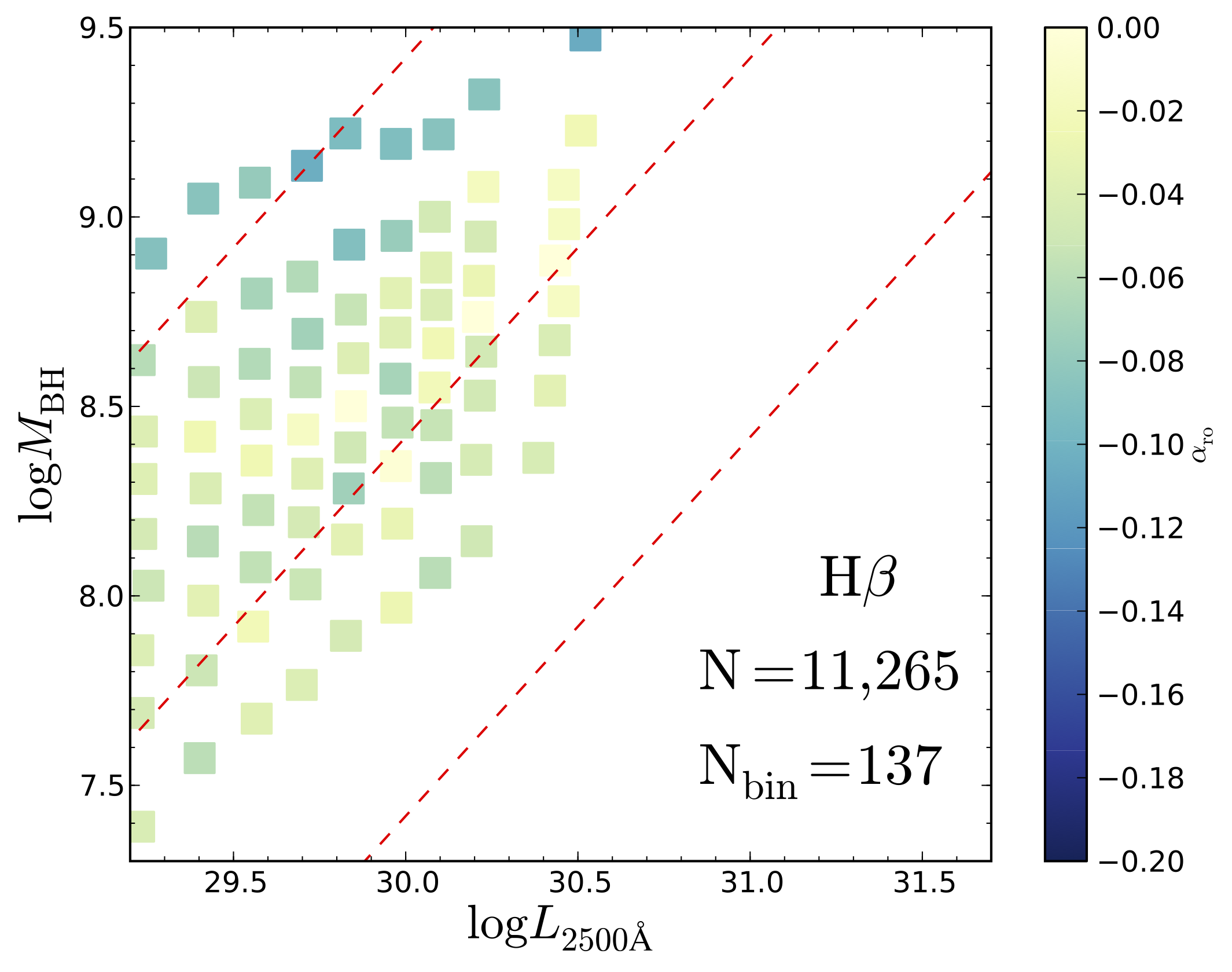
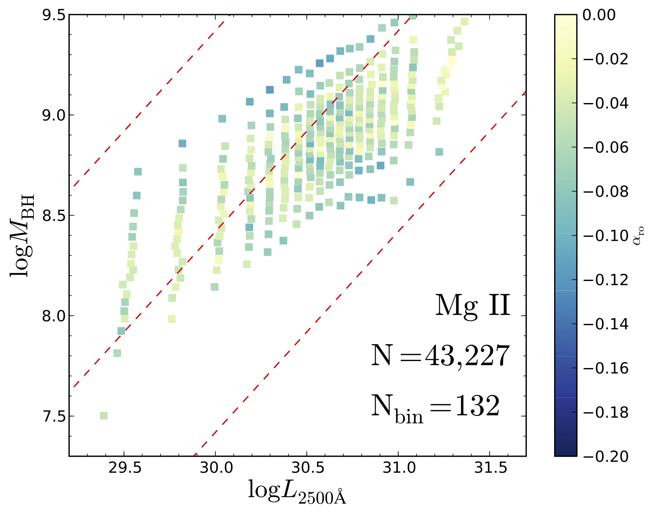
Figure 25: Radio-to-optical spectral indices ($\alpha_{\rm ro}$) of stacked quasar cutouts in BH mass parameter space for optically detected quasars within the FIRST observing area for Sample B (Left: H$\beta$ masses; Right: Mg II masses). The dashed red lines from top-left to bottom right show where $L/L_{\rm Edd}=0.01$, $0.1$, and $1$, in order. We assume $L_{\rm Bol}=2.75L_{\rm 2500\,\AA}$ (Krawczyk et al., 2013).

4.4 The Mean Radio Properties as a Function of Color

We extend our study of the mean radio properties of quasars by exploring the correlation between the strength of radio emission and optical color. As before, we split our samples into bins based on the colors of optically-detected quasars and apply the median stacking procedure described above. Similar to White et al. (2007, Fig. 14), we will use $\Delta(g-i)$ for our measure of color. As stated earlier, $\Delta(g-i)$ is defined in such a way to remove the dependence of color on redshift. It is roughly equivalent to $\alpha_{\rm opt}$, the underlying continuum (excluding emission features) in the optical-UV part of the SED.

Figure 26 shows how median radio flux density varies as a function of color. Just as in White et al. (2007), we find that bluer and redder objects have higher radio flux densities with the reddest objects being the brightest of all. We find that objects with $\Delta(g-i)>0.6$ have peak flux densities 2-3 times larger than quasars with average colors.

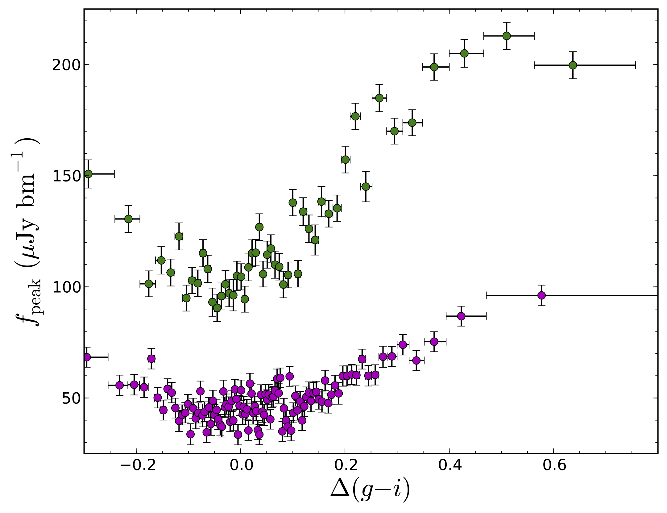
Figure 26: Radio fluxes of stacked quasar cutouts as a function of $\Delta(g-i)$ with samples as in Fig. 11.

As we wish to analyze the intrinsic properties of quasars, we naturally examined how radio luminosity changes with optical color. Figure 27 shows that, for each of our samples, radio luminosity increases for redder objects. Thus, the trend in flux density seen at both color extremes in Figure 26 and in White et al. (2007) appears to be artificial: the blue objects simply have very different luminosities than the red objects.

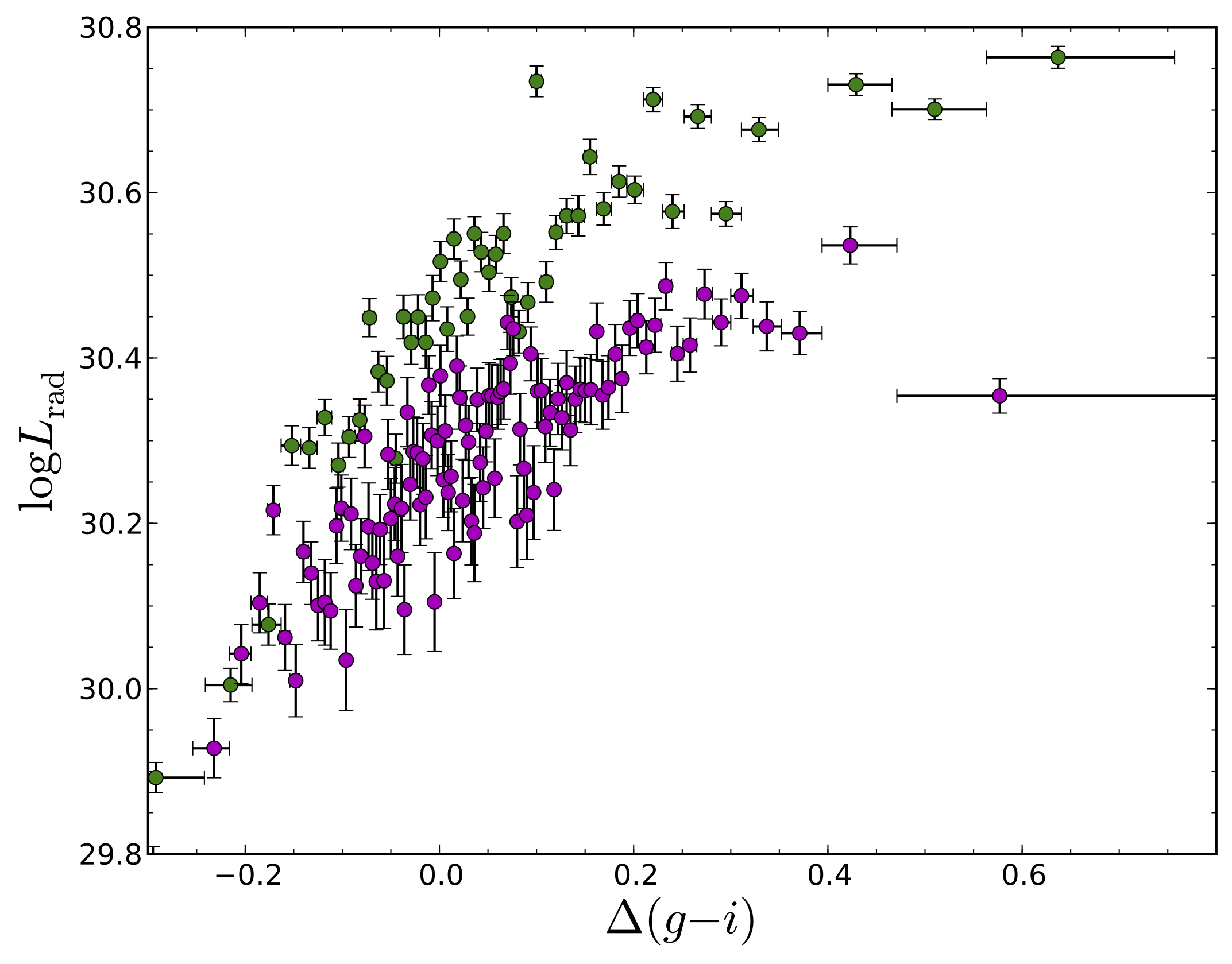
Figure 27: Radio luminosities ($\rm{erg}\,\rm{s}^{-1}\,\rm{Hz}^{-1}$) of stacked quasar cutouts as a function of $\Delta(g-i)$ (Sample B: green; Sample D: purple).

We can quantify the luminosity-corrected trend, instead, by plotting $\alpha_{\rm ro}$ as a function of $\Delta(g-i)$. Figure 28 shows that radio-loudness increases for redder quasars (recall that more radio-loud corresponds to increasingly negative values of $\alpha_{\rm ro}$). As $\alpha_{\rm{ro}}\,$ represents another way to measure the $\log{R}$ parameter (Section 2.7), our results agree with those of White et al. (2007), who found an increase in the $R$-parameter for objects with redder colors.

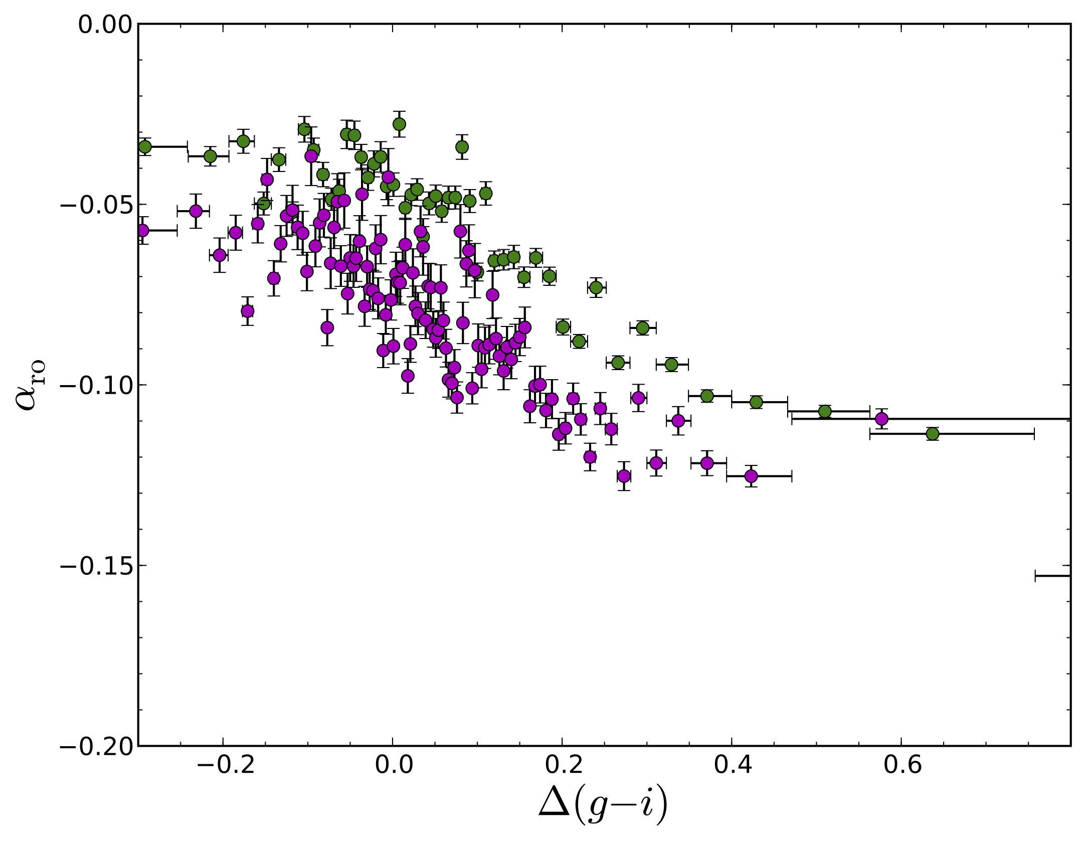
Figure 28: Radio to optical spectral indices ($\alpha_{\rm ro}$) of stacked quasar cutouts as a function of $\Delta(g-i)$ (Sample B: green; Sample D: purple).

These trends match our results from Figures 26 and 27 since objects with increasing radio flux and luminosity should be radio-louder if optical luminosity remains the same. While we expect to measure less optical emission for redder objects because of dust extinction (which does not reduce observed radio emission), optical extinction by dust does not appear to be the lone cause of this trend as it also applies to relatively blue quasars.

5 Discussion

5.1 Mass, Accretion Rate, and Spin

We first consider our results in the context of theoretical work on the relationship between spin, mass, and accretion rate in AGNs. Blandford & Znajek (1977) and Blandford & Payne (1982) provide the framework for how we think the spin of the BH and the accretion disk, respectively, can be tapped in the production of radio jets. Wilson & Colbert (1995) argue that $M_{\rm BH}$ and $\dot{M}$ are not that different for RL and RQ quasars and that the difference must be related to the spin. Both Zamfir et al. (2008) and Richards et al. (2011) also argue for a similarity of properties between RL and at least part of the RQ population.

Previous work has suggested that the radio-loudness is dependent on either the black hole mass or the accretion rate. For example, Laor (2000) and Lacy et al. (2001) find that high BH mass is a necessary (if insufficient) condition for being radio-loud and that there is also a (weaker) correlation with $L/L_{\rm{Edd}}$. Woo & Urry (2002), on the other hand, argue that there is no dependence on BH mass. Ho (2002) similarly finds little BH mass dependence and argues instead for $L/L_{\rm{Edd}}$ as the primary driver; however, Jarvis & McLure (2002) claim that the use of $R$, rather than $L_{\rm rad}$, by Ho (2002) to characterize quasars as RL or RQ led to the uncorrelated results. Jarvis & McLure (2002) also assert that doppler boosting brightens the intrinsic $L_{\rm rad}$ of flat spectrum sources and that the corrected data agrees with a dependence of the form $L_{\rm rad}\propto M_{\rm BH}^{2.5}$ (Dunlop et al., 2003). Sikora et al. (2007), using a sample that is largely complementary to ours, found that radio-loudness increases with decreasing $L/L_{\rm{Edd}}$ but argued that there must also be a secondary parameter (BH mass or spin) in effect. Based on a PCA analysis, Boroson (2002) presents a schematic in which RL quasars preferentially have both high BH mass and low $L/L_{\rm{Edd}}$.

Our results (Figures 23–25) lead us to a very different conclusion than that of Shankar et al. (2010) (using much of the same data) who find that high-redshift RL quasars have high $L/L_{\rm{Edd}}$, while low-redshift RL quasars have low $L/L_{\rm{Edd}}$. This difference is because we consider the BH masses of the high-redshift quasars to be in error. After reconsidering the BH masses estimated using the C IV emission line, we find that our results are in general agreement with most of the investigations above: there is a clear trend towards a higher RLF and a louder mean $\alpha_{\rm{ro}}\,$ with decreasing $L/L_{\rm{Edd}}$. However, Figure 24 suggests that the most RL sources at high luminosities do not have particularly low $L/L_{\rm{Edd}}$ in the absolute sense: they are simply the objects with the lowest $L/L_{\rm{Edd}}$ (and thus the highest BH masses) at that luminosity. This finding may suggest that BH mass is the dominant effect and that low $L/L_{\rm{Edd}}$ is a consequence of the mass trend. Moreover, the very different RLF behavior at high and low redshift provide independent evidence that BH masses determined from C IV should be used with extreme caution.

Whatever controls the radio strength of quasars, we cannot lose sight of the fact that, even where RL quasars are most prevalent, the vast majority of the quasars would still be classified as RQ. Thus, whether or not the radio-loudness distribution is bimodal, there is still a strong dichotomy between RL and RQ quasars. This is intriguing as the SDSS quasar targeting and spectroscopic classification is such that we might expect our samples to be predominantly comprised of massive, bulge-dominated systems (Floyd et al., 2004). Consequently, it is worth noting that our quasar sample still shows some of the radio dichotomy of the samples that cover a wider range of luminosity space such as Sikora et al. (2007).

We note that Floyd et al. (2004) found both the RL and RQ quasars (with $M_{V}<-24$ and $z\sim 0.4$) in their investigation to be bulge-dominated systems and that Sikora et al. (2007) found luminous RQ quasars hosted by ellipticals. Specifically, while it has been long known that RL quasars live in ellipticals, Floyd et al. (2004) demonstrates that ellipticals can host RQ quasars too. If luminous, high-redshift quasars are predominantly fueled by major mergers, it must be the case that the average quasar hosted by an elliptical galaxy is RQ. As such, the RL/RQ dichotomy among luminous quasars is unlikely to be entirely due to morphology. While we cannot say with certainty that both extrema of the RQ quasar distribution have the same hosts, there is no compelling reason (other than the differences in radio properties) to think that RL quasars and the RQ quasars that occupy the RL parameter space have different hosts. Although it has been found that RL and RQ quasars have different environments (Malkan, 1984; Smith et al., 1986; Sikora et al., 2007), with RL quasars living in denser regions, such work has only been done in the context of RL vs. RQ as a whole. In that case, we would indeed expect there to be differences. What would be of more interest is to redo environmental and clustering studies considering RL quasars in comparison with different subsets of RQ quasars, specifically dividing up RQ quasars into hard-spectrum RQs (HSRQs; which may have similar properties as RL quasars) and soft-spectrum RQs (SSRQs; which would be expected to have the largest environmental and clustering differences in comparison with RL quasars).

If massive, low $L/L_{\rm{Edd}}$ systems can be both RL and RQ and if morphology and/or environment are not clearly different between RL quasars and their (putative) parent RQ quasars, then we are left to consider spin as the defining parameter. Major mergers (that are hypothesized to be the dominant cause of the luminous quasars in our investigation) are expected to produce high-spin systems (Wilson & Colbert, 1995; Volonteri et al., 2007, 2013). In part, this is because if enough matter is accreted in one feeding (and even if the accretion is initially retrograde) the BH is spun down more efficiently than it is spun up; this tends to drive quasars that have experienced a recent major merger to high (prograde) spin (Volonteri et al., 2013). This leads to a paradox: if RL quasars have high spin and RQ quasars are not spinning (e.g., Wilson & Colbert 1995), then the accretion efficiency suggested by the Soltan (1982) argument means that RL quasars should not be as rare as they are. This further argues against RL quasars having retrograde spin as in Garofalo (2009) and Garofalo et al. (2010).

One way to reconcile all of this is if both the RL quasars and those RQ quasars with otherwise similar properties (i.e., HSRQs) are dominated by major mergers, resulting in elliptical hosts with high spins. These are systems with high mass for their luminosity and low $L/L_{\rm{Edd}}$. The quasars among these that become RL may be those that have undergone a rare “2nd generation merger” and have been spun up to a value above some threshold (Sikora, 2009). However, we note that the spins are not likely to be all that different as significant differences in the spin would lead to significant changes in the accretion disk properties (in particular the inner radius) that would be expected to produce continuum (and broad emission line region) changes inconsistent with the results of Richards et al. (2011).

This suggests that RL quasars and HSRQ quasars both have high spin, with the RL quasars being somewhat more extreme. The rest of the RQ population (SSRQs) could be similarly high spin objects, may have decreasing spin with increasing $L/L_{\rm{Edd}}$, or could have no spin. Again, however, the Soltan (1982) argument would suggest that having some spin is more likely than having no spin.

In terms of making connections to low-$z$ quasars, it is particularly important to realize that low-$z$ quasars (that are the frequent focus of detailed observing campaigns and reverberation mapping analysis) and the luminous high-$z$ quasars that dominate our sample might be rather different creatures, especially if low-$z$ quasars are primarily accreting molecular clouds (Volonteri et al., 2013). This might explain the somewhat different results seen here and by Boroson (2002) in terms of whether or not RL quasars are an extrema of the quasar population in ways other than in the radio. While we can confirm the finding of Boroson (2002) that RL quasars tend to be high mass, low $L/L_{\rm{Edd}}$ sources, we do not find them to be unique. Indeed most high mass, low $L/L_{\rm{Edd}}$ quasars are RQ.

5.2 Accretion Disk Winds

Our analyses in Eigenvector 1 and C IV parameter spaces (Section 4.2) and even color space (Section 4.4) paint a consistent picture in that we find different quasar properties tracking together. For example, Sulentic et al. (2007) find a correlation between the C IV blueshift and R(Fe II), Reichard et al. (2003) find a correlation between C IV blueshift and quasar color, we find a correlation between radio loudness and color (Fig. 28), while both Gallagher et al. (2005) and Kruczek et al. (2011) consider the connection between X-ray properties and C IV emission. The mean and extreme radio properties in these parameter spaces track together such that higher RLF and higher mean radio-loudness are biased to low blueshifts (Figure 22). More specifically, radio-loud quasars exhibit behaviors (emission line and continuum properties) that are consistent with one extreme (large H$\beta$ FWHM, low R(Fe II), small C IV blueshift, red color) being much more likely to host quasars with stronger radio emission than the opposite. This result is in agreement with the investigation by Zamfir et al. (2008).

If the C IV blueshift is related to the strength of a radiation line-driven wind, this finding is very interesting in terms of the long-observed anti-correlation between radio-loud quasars and BALQSOs (Broad Absorption Line QSOs; Stocke et al. 1992). While sources with strong radio lobes tend to avoid BALQSOs (or vice versa) (Stocke et al., 1992; Reichard et al., 2003; Richards et al., 2011), they are not mutually exclusive (Becker et al., 2000; Welling et al., 2014). In the Richards et al. (2011) picture, all quasars have some sort of wind; it is just that objects displaying absorption troughs that meet the traditional BALQSO definition will have stronger radiation line-driven winds than quasars that do not. Further, Richards et al. (2011) argue that emission line properties can be used to determine the strength of radiation line-driving and, thus, of seeing BAL troughs along other lines of sight. As high $L/L_{\rm{Edd}}$ might be most expected to lead to a strong radiation line-driven wind, the general anti-correlation of BALQSOs and RL quasars would be expected.

Second generation quasars in the model of Sikora (2009) could explain the existence of the rare RL BALQSOs. RL BALQSOs could be those BALQSOs undergoing a “2nd major merger” (Sikora, 2009) and getting spun up enough to produce a radio jet or, alternatively, those RL quasars which undergo a significant increase in accretion rate that generates a radiation line-driven wind. Another possibility is that RL BALQSOs could be related to radio emission resulting from interactions between their outflows and the ISM (Jiang et al., 2010; Zakamska & Greene, 2014).

5.3 Evolution in $L$ and $z$

While the trends in the RLF as a function of mass, accretion rate, and wind-dominance seem clear, it is frustrating that we are not able to better constrain the evolution in optical luminosity and redshift. It is curious that, unlike in the $L$-$z$ parameter space (where the mean and extreme radio properties of quasars run in opposite directions), in the EV1 (Figure 21), C IV (Figure 22), and BH (Figures 24 and 25) parameter spaces the RLF and mean radio-loudness increase in the same direction. Specifically, we see reasonable agreement between the directions of evolution of the mean radio-loudness and the RLF when we are considering parameters that are not a strong function of the apparent magnitude. As a result, an explanation for the differences seen in the $L$-$z$ evolution could be the incompleteness of the FIRST survey (see Section 2.6.5) assuming that the incompleteness is (indirectly) a function of optical magnitude. In this case, the relative shallowness of the radio data could be masking the true $L-z$ evolution of the RLF.

While it would seem that the mean radio loudness from stacking is more robust, Figure 13 showed that optically fainter quasars have $\alpha_{\rm{ro}}\,$ values that are more radio loud, which could indicate a bias in the stacking results instead. Such a correlation could come about if bright quasars that are extincted by dust are moving to larger (fainter) magnitudes and, thus, appear to be more RL than they should be. However, we have excluded quasars that are most heavily dust reddened/extincted, $\Delta(g-i)>0.5$, and we have further argued using Figure 19 that dust is unlikely to be dominating the trend.

In short, modulo any corrections for the $L$- and $z$-dependences of $\alpha_{\rm{ro}}\,$, we are left to conclude that the mean radio-loudness does indeed evolve with both redshift and luminosity in a way that mimics a trend in apparent magnitude. The opposite trend of the RLF with apparent magnitude is either also real or is an artifact of incompleteness to RL objects with fainter magnitude. We note that there is no reason that the RLF and the mean radio-loudness have to evolve together in either $L$ or $z$, but the similarity of the trends in the other parameter spaces that we have considered may suggest that the observed RLF evolution is less robust than evolution of the mean radio loudness. Both deeper radio observations within the SDSS/FIRST footprint and observations targeted at objects at the extremes of $L-z$ parameter space (e.g., high-$z$ quasars) would help to answer this important question.

5.4 On the Meaning of Radio-Quiet

Our goal was to identify non-radio properties of quasars that could be used to predict whether an individual quasar is likely to be a strong radio source or not. In that sense we have failed: RL quasars and at least some RQ quasars do not appear to be significantly different. That said, we have expanded the parameter space over which the RL/RQ dichotomy has been thoroughly investigated and have identified properties that suggest when an optical quasar is very unlikely to be a strong radio source. To make further progress, it would help to be able to estimate BH spins for large samples of (distant) quasars.

Given the relative similarity of RL and (some) RQ quasars, we emphasize that there is no such thing as a “radio-quiet” quasar. We mean this literally in that all quasars appear to have some minimum level of radio flux based on direct detections from deep observations (Kimball et al., 2011) and hinted at by stacking (Figure 14 and White et al. 2007) and demographic analyses (Condon et al., 2013). However, we also mean it figuratively in that the RQ population spans a large range of continuum and emission line properties (e.g., Sulentic et al. 2000b and Richards et al. 2011) such that it cannot be considered a single monolithic object class. For example, Richards et al. (2011) compared the average RL quasar spectrum to the average spectrum of RQs with similar C IV EQWs and low blueshifts and found little difference, whereas composite spectra from the other extreme in the RQ population have quite different emission line properties.

Sulentic et al. (2000b) and collaborators have emphasized this finding by dividing quasars into “Population A” and “Population B”. In Kruczek et al. (2011) we give these classes more physical meaning by refering to them as, respecively, “soft-spectrum” and “hard-spectrum” sources—especially when referring to RQ quasars where the extrema (within the continuum) can be denoted as hard-spectrum radio quiet (HSRQ) and soft-spectrum radio quiet (SSRQ).

We argue that investigations that have naively split the quasar population into two (RL/RQ) should be reconsidered. If a RL sample is compared to a truly representative RQ sample, one would expect to see differences since the RQ population spans a larger range of parameter space than the RL. Comparisons of RL quasars separately with what we have called HSRQ and SSRQs quasars would be extremely interesting.

6 Conclusions

In Section 1 we argued that the seemingly discordant literature on the possible bimodality of the detected quasar population is actually in good agreement. All investigations find that the distribution of radio-loudness is poorly fit by a single component: there is a minority population of radio-loud objects. As noted by Laor (2003), evolution of this population may cloud our analysis of it through the use of a single dividing line at all redshifts and luminosities.

Section 2.7 explains why we adopt $\alpha_{\rm{ro}}\,$ as our measure of radio-loudness instead of $\log R$. Although $\log R$ has been commonly used among radio astronomers, we have decided to implement $\alpha_{\rm{ro}}\,$ in our analyses to make our results accessible to those who do not primarily work within the radio regime. $\alpha_{\rm{ro}}\,$ is universal in that it directly describes the shape of a quasar’s spectral energy distribution, specifically between the radio and the optical.

In Section 4.1 (Figure 20) we showed that the radio-loud fraction appears to evolve in both $L$ and $z$, in agreement with Jiang et al. (2007) and Baloković et al. (2012). This evolution is such that the RLF most closely tracks the optical apparent magnitude, which suggests a possible bias. A radio sample covering the area of the FIRST survey to 3$\times$ its depth or deeper is needed to resolve this issue. We further found that the mean radio-loudness evolves in the exact opposite sense. Thus, it appears that the mean and extrema of the radio-loudness distribution do not track each other. This difference could offer insight into the nature of radio emission in quasars, perhaps suggesting different tracks for the RL and radio-intermediate sources. Alternatively, it could be an indication that FIRST is indeed incomplete in a manner that clouds our understanding of the RLF evolution.

We explored the evolution of radio properties in Eigenvector 1 and C IV parameter spaces in Section 4.2. These properties may trace the relative power of radiation line-driven accretion disk winds (Richards et al., 2011). The RLF is much higher in quasars without emission properties that point to strong radiation line-driven winds. Indeed, the RLF is essentially zero for quasars with the highest C IV blueshifts (Figure 22). The mean radio-loudness shows a similar, albeit somewhat weaker, trend. The trends in RLF and mean radio-loudnessin EV1 parameter space (Figure 21) are broadly consistent with the C IV results. We further find that the mean radio-loudness increases with increasing reddening of the optical continuum (Figure 28), which is consistent with these other findings. Contrary to Boroson (2002), we find that while RL quasars tend occupy only a fraction of the quasar parameter space, they not occupy a unique parameter space; thus, it appears that RL and RQ quasars are parallel sequences. Some additional parameter (spin?) must contribute to an object being RL, where that parameter is strongly biased to those objects without strong radiation line-driven winds.

Section 4.3 considers the radio properties of quasars as a function of mass, accretion rate, and $L/L_{\rm{Edd}}$. We argue that BH mass estimates from survey-quality spectral measurements of C IV have catastrophic errors in luminous quasars. This finding is relevant to other investigation of BH masses in high-redshift quasars. These errors are identified by a radical change in the radio properties of quasars as a function of BH mass with redshift and have led some previous work to questionable conclusions regarding the redshift evolution of $L/L_{\rm{Edd}}$ for RL quasars. Ignoring the biased C IV BH mass results (or assuming that the actual C IV BH masses are inverted from their apparent values), we find that the radio-loud fraction is highest for the largest BH masses (at a given luminosity) (Figure 24). This means that the RLF is a function of $L/L_{\rm{Edd}}$, in agreement with past results. The mean radio-loudness shows a similar, but somewhat weaker trend.

Further progress must come in the context of the realization that there is no typical RQ quasar with which to contrast the RL population. Rather RL quasars should be compared to RQ quasars that have similar (non-radio) properties (Population B in Sulentic et al. 2000a, b and HSRQ in Kruczek et al. 2011) and contrasted with those RQ quasars that exhibit dissimilar (non-radio) properties (Population A in Sulentic et al. 2000a, b and SSRQ in Kruczek et al. 2011). As we find little to differentiate RL quasars and HSRQs, the suggestion by Sikora et al. (2007) of RL quasars being spun-up by second generation mergers is an intriguing one.

References

- Abazajian et al. (2009) Abazajian, K. N., et al. 2009, ApJS, 182, 543, 0812.0649
- Ahn et al. (2012) Ahn, C. P., et al. 2012, ApJS, 203, 21, 1207.7137
- Assef et al. (2011) Assef, R. J., et al. 2011, ApJ, 742, 93, 1009.1145
- Avni & Tananbaum (1982) Avni, Y. & Tananbaum, H. 1982, ApJ, 262, L17
- Baloković et al. (2012) Baloković, M., Smolčić, V., Ivezić, Ž., Zamorani, G., Schinnerer, E., & Kelly, B. C. 2012, ApJ, 759, 30, 1209.1099
- Barthel (1989) Barthel, P. D. 1989, ApJ, 336, 606
- Barvainis et al. (2005) Barvainis, R., Lehár, J., Birkinshaw, M., Falcke, H., & Blundell, K. M. 2005, ApJ, 618, 108, astro-ph/0409554
- Becker et al. (2000) Becker, R. H., White, R. L., Gregg, M. D., Brotherton, M. S., Laurent-Muehleisen, S. A., & Arav, N. 2000, ApJ, 538, 72, astro-ph/0002470
- Becker et al. (1995) Becker, R. H., White, R. L., & Helfand, D. J. 1995, ApJ, 450, 559
- Blandford (1990) Blandford, R. D. 1990, in Active Galactic Nuclei, eds. R. D. Blandford, H. Netzer, L. Woltjer, T. J.-L. Courvoisier, & M. Mayor, 161–275
- Blandford & Payne (1982) Blandford, R. D. & Payne, D. G. 1982, MNRAS, 199, 883
- Blandford & Znajek (1977) Blandford, R. D. & Znajek, R. L. 1977, MNRAS, 179, 433
- Blanton et al. (2003) Blanton, M. R., et al. 2003, ApJ, 592, 819, arXiv:astro-ph/0210215
- Blundell & Beasley (1998) Blundell, K. M. & Beasley, A. J. 1998, MNRAS, 299, 165, astro-ph/9805169
- Blundell & Kuncic (2007) Blundell, K. M. & Kuncic, Z. 2007, ApJ, 668, L103, 0708.2929
- Bondi et al. (2008) Bondi, M., Ciliegi, P., Schinnerer, E., Smolčić, V., Jahnke, K., Carilli, C., & Zamorani, G. 2008, ApJ, 681, 1129, 0804.1706
- Boroson (2002) Boroson, T. A. 2002, ApJ, 565, 78, astro-ph/0109317
- Boroson & Green (1992) Boroson, T. A. & Green, R. F. 1992, ApJS, 80, 109
- Bovy et al. (2011) Bovy, J., et al. 2011, ApJ, 729, 141, 1011.6392
- Brotherton & Francis (1999) Brotherton, M. S. & Francis, P. J. 1999, in Quasars and Cosmology, eds. G. Ferland & J. Baldwin, vol. 162 of Astronomical Society of the Pacific Conference Series, 395, astro-ph/9811088
- Casebeer et al. (2006) Casebeer, D. A., Leighly, K. M., & Baron, E. 2006, ApJ, 637, 157, arXiv:astro-ph/0508503
- Cirasuolo et al. (2003a) Cirasuolo, M., Celotti, A., Magliocchetti, M., & Danese, L. 2003a, MNRAS, 346, 447, astro-ph/0306415
- Cirasuolo et al. (2003b) Cirasuolo, M., Magliocchetti, M., Celotti, A., & Danese, L. 2003b, MNRAS, 341, 993, astro-ph/0301526
- Condon et al. (2002) Condon, J. J., Cotton, W. D., & Broderick, J. J. 2002, AJ, 124, 675
- Condon et al. (1998) Condon, J. J., Cotton, W. D., Greisen, E. W., Yin, Q. F., Perley, R. A., Taylor, G. B., & Broderick, J. J. 1998, AJ, 115, 1693
- Condon et al. (2013) Condon, J. J., Kellermann, K. I., Kimball, A. E., Ivezić, Ž., & Perley, R. A. 2013, ApJ, 768, 37
- Croom et al. (2004) Croom, S. M., Smith, R. J., Boyle, B. J., Shanks, T., Miller, L., Outram, P. J., & Loaring, N. S. 2004, MNRAS, 349, 1397, arXiv:astro-ph/0403040
- Croom et al. (2009) Croom, S. M., et al. 2009, MNRAS, 392, 19, 0810.4955
- Denney (2012) Denney, K. D. 2012, ApJ, 759, 44, 1208.3465
- Denney et al. (2013) Denney, K. D., Pogge, R. W., Assef, R. J., Kochanek, C. S., Peterson, B. M., & Vestergaard, M. 2013, ApJ, 775, 60, 1303.3889
- Dunlop et al. (2003) Dunlop, J. S., McLure, R. J., Kukula, M. J., Baum, S. A., O’Dea, C. P., & Hughes, D. H. 2003, MNRAS, 340, 1095, astro-ph/0108397
- Edge et al. (1959) Edge, D. O., Shakeshaft, J. R., McAdam, W. B., Baldwin, J. E., & Archer, S. 1959, MmRAS, 68, 37
- Elvis (2000) Elvis, M. 2000, ApJ, 545, 63, arXiv:astro-ph/0008064
- Elvis et al. (1994) Elvis, M., et al. 1994, ApJS, 95, 1
- Fine et al. (2010) Fine, S., Croom, S. M., Bland-Hawthorn, J., Pimbblet, K. A., Ross, N. P., Schneider, D. P., & Shanks, T. 2010, MNRAS, 409, 591, 1005.5287
- Floyd et al. (2004) Floyd, D. J. E., Kukula, M. J., Dunlop, J. S., McLure, R. J., Miller, L., Percival, W. J., Baum, S. A., & O’Dea, C. P. 2004, MNRAS, 355, 196, astro-ph/0308436
- Fukugita et al. (1996) Fukugita, M., Ichikawa, T., Gunn, J. E., Doi, M., Shimasaku, K., & Schneider, D. P. 1996, AJ, 111, 1748
- Gallagher et al. (2005) Gallagher, S. C., Richards, G. T., Hall, P. B., Brandt, W. N., Schneider, D. P., & Vanden Berk, D. E. 2005, AJ, 129, 567, astro-ph/0410641
- Garofalo (2009) Garofalo, D. 2009, ApJ, 699, L52, 0905.4782
- Garofalo et al. (2010) Garofalo, D., Evans, D. A., & Sambruna, R. M. 2010, MNRAS, 406, 975, 1004.1166
- Gaskell (1982) Gaskell, C. M. 1982, ApJ, 263, 79
- Glikman et al. (2006) Glikman, E., Helfand, D. J., & White, R. L. 2006, ApJ, 640, 579, arXiv:astro-ph/0511640
- Goldschmidt et al. (1999) Goldschmidt, P., Kukula, M. J., Miller, L., & Dunlop, J. S. 1999, ApJ, 511, 612, arXiv:astro-ph/9810392
- Gunn et al. (1998) Gunn, J. E., et al. 1998, AJ, 116, 3040, arXiv:astro-ph/9809085
- Gunn et al. (2006) — 2006, AJ, 131, 2332, arXiv:astro-ph/0602326
- Hewett & Wild (2010) Hewett, P. C. & Wild, V. 2010, MNRAS, 405, 2302, 1003.3017
- Ho (2002) Ho, L. C. 2002, ApJ, 564, 120, astro-ph/0110440
- Hodge et al. (2011) Hodge, J. A., Becker, R. H., White, R. L., Richards, G. T., & Zeimann, G. R. 2011, AJ, 142, 3, 1103.5749
- Hogg et al. (2001) Hogg, D. W., Finkbeiner, D. P., Schlegel, D. J., & Gunn, J. E. 2001, AJ, 122, 2129, astro-ph/0106511
- Ivezić et al. (2002) Ivezić, Ž., et al. 2002, AJ, 124, 2364, arXiv:astro-ph/0202408
- Ivezić et al. (2004) — 2004, Astronomische Nachrichten, 325, 583, astro-ph/0410195
- Jarvis & McLure (2002) Jarvis, M. J. & McLure, R. J. 2002, MNRAS, 336, L38, astro-ph/0208390
- Jester (2005) Jester, S. 2005, ApJ, 625, 667, astro-ph/0502394
- Jiang et al. (2007) Jiang, L., Fan, X., Ivezić, Ž., Richards, G. T., Schneider, D. P., Strauss, M. A., & Kelly, B. C. 2007, ApJ, 656, 680, arXiv:astro-ph/0611453
- Jiang et al. (2010) Jiang, Y.-F., Ciotti, L., Ostriker, J. P., & Spitkovsky, A. 2010, ApJ, 711, 125, 0904.4918
- Just et al. (2007) Just, D. W., Brandt, W. N., Shemmer, O., Steffen, A. T., Schneider, D. P., Chartas, G., & Garmire, G. P. 2007, ApJ, 665, 1004, 0705.3059
- Kellermann et al. (1989) Kellermann, K. I., Sramek, R., Schmidt, M., Shaffer, D. B., & Green, R. 1989, AJ, 98, 1195
- Kimball & Ivezić (2008) Kimball, A. E. & Ivezić, Ž. 2008, AJ, 136, 684, 0806.0650
- Kimball et al. (2011) Kimball, A. E., Kellermann, K. I., Condon, J. J., Ivezić, Ž., & Perley, R. A. 2011, ApJ, 739, L29, 1107.3551
- Kochanek et al. (2012) Kochanek, C. S., et al. 2012, ApJS, 200, 8, 1110.4371
- Krawczyk et al. (2013) Krawczyk, C. M., Richards, G. T., Mehta, S. S., Vogeley, M. S., Gallagher, S. C., Leighly, K. M., Ross, N. P., & Schneider, D. P. 2013, ApJS, 206, 4, 1304.5573
- Kruczek et al. (2011) Kruczek, N. E., et al. 2011, AJ, 142, 130, 1109.1515
- Lacy et al. (2001) Lacy, M., Laurent-Muehleisen, S. A., Ridgway, S. E., Becker, R. H., & White, R. L. 2001, ApJ, 551, L17, astro-ph/0103087
- Laor (2000) Laor, A. 2000, ApJ, 543, L111, astro-ph/0009192
- Laor (2003) — 2003, ArXiv Astrophysics e-prints, astro-ph/0312417
- Leighly (2004) Leighly, K. M. 2004, ApJ, 611, 125, arXiv:astro-ph/0402452
- Leighly et al. (2007) Leighly, K. M., Halpern, J. P., Jenkins, E. B., Grupe, D., Choi, J., & Prescott, K. B. 2007, ApJ, 663, 103, arXiv:astro-ph/0611349
- Lilly et al. (2007) Lilly, S. J., et al. 2007, ApJS, 172, 70, arXiv:astro-ph/0612291
- Lupton et al. (2001) Lupton, R., Gunn, J. E., Ivezić, Z., Knapp, G. R., & Kent, S. 2001, in Astronomical Data Analysis Software and Systems X, eds. F. R. Harnden, Jr., F. A. Primini, & H. E. Payne, vol. 238 of Astronomical Society of the Pacific Conference Series, 269, astro-ph/0101420
- Lusso et al. (2010) Lusso, E., et al. 2010, A&A, 512, A34, 0912.4166
- Lynden-Bell (1969) Lynden-Bell, D. 1969, Nature, 223, 690
- Maddox et al. (2012) Maddox, N., Hewett, P. C., Péroux, C., Nestor, D. B., & Wisotzki, L. 2012, MNRAS, 424, 2876, 1206.1434
- Mahony et al. (2012) Mahony, E. K., Sadler, E. M., Croom, S. M., Ekers, R. D., Feain, I. J., & Murphy, T. 2012, ApJ, 754, 12, 1205.2233
- Malkan (1984) Malkan, M. A. 1984, ApJ, 287, 555
- McLure & Jarvis (2002) McLure, R. J. & Jarvis, M. J. 2002, MNRAS, 337, 109, astro-ph/0204473
- Miller et al. (2011) Miller, B. P., Brandt, W. N., Schneider, D. P., Gibson, R. R., Steffen, A. T., & Wu, J. 2011, ApJ, 726, 20, 1010.4804
- Miller et al. (1990) Miller, L., Peacock, J. A., & Mead, A. R. G. 1990, MNRAS, 244, 207
- Moore & Stockman (1984) Moore, R. L. & Stockman, H. S. 1984, ApJ, 279, 465
- Murray et al. (1995) Murray, N., Chiang, J., Grossman, S. A., & Voit, G. M. 1995, ApJ, 451, 498
- Neugebauer et al. (1986) Neugebauer, G., Miley, G. K., Soifer, B. T., & Clegg, P. E. 1986, ApJ, 308, 815
- Oke & Gunn (1983) Oke, J. B. & Gunn, J. E. 1983, ApJ, 266, 713
- Palanque-Delabrouille et al. (2013) Palanque-Delabrouille, N., et al. 2013, A&A, 551, A29, 1209.3968
- Papovich et al. (2006) Papovich, C., et al. 2006, AJ, 132, 231, arXiv:astro-ph/0512623
- Pâris et al. (2012) Pâris, I., et al. 2012, A&A, 548, A66, 1210.5166
- Park et al. (2013) Park, D., Woo, J.-H., Denney, K. D., & Shin, J. 2013, ApJ, 770, 87, 1304.7281
- Peacock et al. (1986) Peacock, J. A., Miller, L., & Longair, M. S. 1986, MNRAS, 218, 265
- Pier et al. (2003) Pier, J. R., Munn, J. A., Hindsley, R. B., Hennessy, G. S., Kent, S. M., Lupton, R. H., & Ivezić, Ž. 2003, AJ, 125, 1559, astro-ph/0211375
- Proga et al. (2000) Proga, D., Stone, J. M., & Kallman, T. R. 2000, ApJ, 543, 686, arXiv:astro-ph/0005315
- Rafiee & Hall (2011) Rafiee, A. & Hall, P. B. 2011, MNRAS, 415, 2932, 1011.1268
- Rafter et al. (2009) Rafter, S. E., Crenshaw, D. M., & Wiita, P. J. 2009, AJ, 137, 42, 0809.3977
- Reichard et al. (2003) Reichard, T. A., et al. 2003, AJ, 126, 2594, astro-ph/0308508
- Richards et al. (2002a) Richards, G. T., Vanden Berk, D. E., Reichard, T. A., Hall, P. B., Schneider, D. P., SubbaRao, M., Thakar, A. R., & York, D. G. 2002a, AJ, 124, 1, arXiv:astro-ph/0204162
- Richards et al. (2002b) Richards, G. T., et al. 2002b, AJ, 123, 2945, arXiv:astro-ph/0202251
- Richards et al. (2003) — 2003, AJ, 126, 1131, arXiv:astro-ph/0305305
- Richards et al. (2006) — 2006, AJ, 131, 2766, arXiv:astro-ph/0601434
- Richards et al. (2009) — 2009, ApJS, 180, 67, 0809.3952
- Richards et al. (2011) — 2011, AJ, 141, 167, 1011.2282
- Runnoe et al. (2013) Runnoe, J. C., Brotherton, M. S., Shang, Z., & DiPompeo, M. A. 2013, MNRAS, 434, 848, 1306.3521
- Sanders et al. (1989) Sanders, D. B., Phinney, E. S., Neugebauer, G., Soifer, B. T., & Matthews, K. 1989, ApJ, 347, 29
- Schlegel et al. (1998) Schlegel, D. J., Finkbeiner, D. P., & Davis, M. 1998, ApJ, 500, 525, astro-ph/9710327
- Schmidt (1963) Schmidt, M. 1963, Nature, 197, 1040
- Schmidt (1970) — 1970, ApJ, 162, 371
- Schmidt & Green (1983) Schmidt, M. & Green, R. F. 1983, ApJ, 269, 352
- Schneider et al. (2010) Schneider, D. P., et al. 2010, AJ, 139, 2360, 1004.1167
- Shankar et al. (2010) Shankar, F., Sivakoff, G. R., Vestergaard, M., & Dai, X. 2010, MNRAS, 401, 1869, 0909.4092
- Shen et al. (2011) Shen, Y., et al. 2011, ApJS, 194, 45, 1006.5178
- Sikora (2009) Sikora, M. 2009, Astronomische Nachrichten, 330, 291, 0811.3105
- Sikora et al. (2007) Sikora, M., Stawarz, Ł., & Lasota, J.-P. 2007, ApJ, 658, 815, astro-ph/0604095
- Singal et al. (2011) Singal, J., Petrosian, V., Lawrence, A., & Stawarz, Ł. 2011, ApJ, 743, 104, 1101.2930
- Singal et al. (2013) Singal, J., Petrosian, V., Stawarz, Ł., & Lawrence, A. 2013, ApJ, 764, 43, 1207.3396
- Smith et al. (1986) Smith, E. P., Heckman, T. M., Bothun, G. D., Romanishin, W., & Balick, B. 1986, ApJ, 306, 64
- Soltan (1982) Soltan, A. 1982, MNRAS, 200, 115
- Spergel et al. (2007) Spergel, D. N., et al. 2007, ApJS, 170, 377, astro-ph/0603449
- Steffen et al. (2006) Steffen, A. T., Strateva, I., Brandt, W. N., Alexander, D. M., Koekemoer, A. M., Lehmer, B. D., Schneider, D. P., & Vignali, C. 2006, AJ, 131, 2826, arXiv:astro-ph/0602407
- Steidel & Sargent (1991) Steidel, C. C. & Sargent, W. L. W. 1991, ApJ, 382, 433
- Stocke et al. (1992) Stocke, J. T., Morris, S. L., Weymann, R. J., & Foltz, C. B. 1992, ApJ, 396, 487
- Stoughton et al. (2002) Stoughton, C., et al. 2002, AJ, 123, 485
- Strittmatter et al. (1980) Strittmatter, P. A., Hill, P., Pauliny-Toth, I. I. K., Steppe, H., & Witzel, A. 1980, A&A, 88, L12
- Sulentic et al. (2007) Sulentic, J. W., Bachev, R., Marziani, P., Negrete, C. A., & Dultzin, D. 2007, ApJ, 666, 757, 0705.1895
- Sulentic et al. (2000a) Sulentic, J. W., Marziani, P., & Dultzin-Hacyan, D. 2000a, ARA&A, 38, 521
- Sulentic et al. (2000b) Sulentic, J. W., Zwitter, T., Marziani, P., & Dultzin-Hacyan, D. 2000b, ApJ, 536, L5, astro-ph/0005177
- Trump et al. (2009) Trump, J. R., et al. 2009, ApJ, 696, 1195, 0811.3977
- Ulvestad et al. (2005) Ulvestad, J. S., Antonucci, R. R. J., & Barvainis, R. 2005, ApJ, 621, 123, astro-ph/0411678
- Urry & Padovani (1995) Urry, C. M. & Padovani, P. 1995, PASP, 107, 803, arXiv:astro-ph/9506063
- Vanden Berk et al. (2001) Vanden Berk, D. E., et al. 2001, AJ, 122, 549, arXiv:astro-ph/0105231
- Vanden Berk et al. (2005) — 2005, AJ, 129, 2047, astro-ph/0501113
- Vestergaard & Peterson (2006) Vestergaard, M. & Peterson, B. M. 2006, ApJ, 641, 689, %****␣ms_astroph.bbl␣Line␣475␣****astro-ph/0601303
- Visnovsky et al. (1992) Visnovsky, K. L., Impey, C. D., Foltz, C. B., Hewett, P. C., Weymann, R. J., & Morris, S. L. 1992, ApJ, 391, 560
- Volonteri et al. (2007) Volonteri, M., Sikora, M., & Lasota, J.-P. 2007, ApJ, 667, 704, 0706.3900
- Volonteri et al. (2013) Volonteri, M., Sikora, M., Lasota, J.-P., & Merloni, A. 2013, ApJ, 775, 94, 1210.1025
- Wals et al. (2005) Wals, M., Boyle, B. J., Croom, S. M., Miller, L., Smith, R., Shanks, T., & Outram, P. 2005, MNRAS, 360, 453, arXiv:astro-ph/0502401
- Welling et al. (2014) Welling, C. A., Miller, B. P., Brandt, W. N., Capellupo, D. M., & Gibson, R. R. 2014, ArXiv e-prints, 1403.0958
- White et al. (2007) White, R. L., Helfand, D. J., Becker, R. H., Glikman, E., & de Vries, W. 2007, ApJ, 654, 99, arXiv:astro-ph/0607335
- White et al. (2000) White, R. L., et al. 2000, ApJS, 126, 133, astro-ph/9912215
- Wilkes (1984) Wilkes, B. J. 1984, MNRAS, 207, 73
- Wilson & Colbert (1995) Wilson, A. S. & Colbert, E. J. M. 1995, ApJ, 438, 62, astro-ph/9408005
- Wisotzki (2000) Wisotzki, L. 2000, A&A, 353, 861
- Woo & Urry (2002) Woo, J.-H. & Urry, C. M. 2002, ApJ, 581, L5, astro-ph/0211118
- Worseck & Prochaska (2011) Worseck, G. & Prochaska, J. X. 2011, ApJ, 728, 23, 1004.3347
- Wu et al. (2012) Wu, J., Brandt, W. N., Anderson, S. F., Diamond-Stanic, A. M., Hall, P. B., Plotkin, R. M., Schneider, D. P., & Shemmer, O. 2012, ApJ, 747, 10, 1112.2228
- Xu et al. (1999) Xu, C., Livio, M., & Baum, S. 1999, AJ, 118, 1169, astro-ph/9905322
- York et al. (2000) York, D. G., et al. 2000, AJ, 120, 1579, arXiv:astro-ph/0006396
- Zakamska & Greene (2014) Zakamska, N. L. & Greene, J. E. 2014, ArXiv e-prints, 1402.6736
- Zamfir et al. (2008) Zamfir, S., Sulentic, J. W., & Marziani, P. 2008, MNRAS, 387, 856, 0804.0788