A Catalog of Quasar Properties from SDSS DR7
Abstract
We present a compilation of properties of the 105,783 quasars in the SDSS Data Release 7 (DR7) quasar catalog. In this product, we compile continuum and emission line measurements around the H, H, MgII and CIV regions, as well as other quantities such as radio properties, and flags indicating broad absorption line quasars (BALQSOs), disk emitters, etc. We also compile virial black hole mass estimates based on various calibrations. For the fiducial virial mass estimates we use the Vestergaard & Peterson (VP06) calibrations for H and CIV, and our own calibration for MgII which matches the VP06 H masses on average. We describe the construction of this catalog, and discuss its limitations. The catalog and its future updates will be made publicly available online.
Subject headings:
black hole physics — galaxies: active — quasars: general — surveys1. Introduction
In recent years, studies of quasars and active galactic nuclei (AGNs) have been greatly facilitated by dedicated large-scale wide and deep field surveys in different bands, most notably by optical surveys such as the Sloan Digital Sky Survey (SDSS, York et al., 2000) and the 2QZ survey (Croom et al., 2004). Indeed, the growing body of data has revolutionized the study of quasars and AGNs. Large, homogeneous data sets allow detailed investigations of the phenomenological properties of quasars and AGNs, offering new insights into the central engine powering these objects and their connections to their host galaxies, especially when combined with multi-wavelength coverage. At the same time, it has become important to fit the quasar/AGN population into its cosmological context, i.e., how the supermassive black hole (SMBH) population evolves across cosmic time. These data have led to a coherent picture of the cosmic evolution of the SMBH population within the concordance CDM paradigm (Kauffmann & Haehnelt, 2000; Wyithe & Loeb, 2003; Hopkins et al., 2006, 2008; Shankar et al., 2009; Shen, 2009), where the key observational components include quasar clustering, the luminosity function (LF), the BH mass function, and the correlations between BHs and their host properties. Increasingly larger data sets are offering unique opportunities to measure these properties with unprecedented precision.
In an earlier study of the virial BH mass and Eddington ratio distributions of quasars, we measured spectral properties for the SDSS Data Release 5 (DR5) quasar catalog (Schneider et al., 2007; Shen et al., 2008b). We hereby extend this exercise to the DR7 quasar catalog (Schneider et al., 2010). We now include a more complete compilation than before of quantities from our spectral fits. Our measurements are more sophisticated than the SDSS pipeline outputs in many ways, and are hence of practical value. We describe the parent quasar sample in §2, and the spectral measurements and the catalog format in §3. We discuss possible applications of our measurements in §4. Throughout this paper we use cosmological parameters , and .
2. The Sample
The SDSS uses a dedicated 2.5-m wide-field telescope (Gunn et al., 2006) with a drift-scan camera with 30 CCDs (Gunn et al., 1998) to image the sky in five broad bands (; Fukugita et al., 1996). The imaging data are taken on dark photometric nights of good seeing (Hogg et al., 2001), are calibrated photometrically (Smith et al., 2002; Ivezić et al., 2004; Tucker et al., 2006) and astrometrically (Pier et al., 2003), and object parameters are measured (Lupton et al., 2001; Stoughton et al., 2002). Quasar candidates (Richards et al., 2002a) for follow-up spectroscopy are selected from the imaging data using their colors, and are arranged in spectroscopic plates (Blanton et al., 2003) to be observed with a pair of fiber-fed double spectrographs.
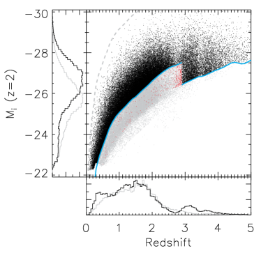
Our parent sample is the latest compilation of the spectroscopic quasar catalog (Schneider et al., 2010) from SDSS DR7 (Abazajian et al., 2009). This sample contains 105,783 bona fide quasars brighter than and have at least one broad emission line with FWHM larger than 1000 or have interesting/complex absorption features. About half of these objects are selected uniformly using the final quasar target selection algorithm described in Richards et al. (2002a), with the remaining objects selected via early versions of the target selection algorithm or various serendipitous algorithms (see Schneider et al., 2010), whose selection completeness cannot be readily quantified. For statistical studies such as quasar clustering and the LF, one should use the uniformly selected quasar sample. Fig. 1 shows the distribution of the 105,783 quasars in the redshift-luminosity plane.
The reduced one-dimensional (1D) spectral data used in this study are available through the SDSS Data Archive Server111http://das.sdss.org/spectro/ (DAS). The spectral resolution is , and the 1D spectra are stored in vacuum wavelength, with a pixel scale of in log-wavelength, which corresponds to . Since the 6th SDSS data release (DR6, Adelman-McCarthy et al., 2008), the spectral flux calibration is scaled to the point spread function (PSF) magnitudes of standard stars, therefore there is no longer need for a fiber-to-PSF conversion for the spectral flux (Shen et al. 2008 also used the PSF spectral flux calibration). Throughout the paper, we refer to the signal-to-noise ratio per pixel as S/N.
To include radio properties, we match the DR7 quasar catalog with the FIRST (White et al., 1997) catalog222The version of the FIRST source catalog and the coverage maps used are as of July 16, 2008 (http://sundog.stsci.edu/first/catalogs/readme.html). with a matching radius of 30” and estimate the radio loudness following Jiang et al. (2007), where and are the flux density () at rest-frame 6 cm and Å, respectively. For the quasars that have only one FIRST source within 30” we match them again to the FIRST catalog with a matching radius 5” and classify the matched ones as core-dominant radio quasars. Those quasars that have multiple FIRST source matches within 30” are classified as lobe-dominated. The rest-frame 6 cm flux density is determined from the FIRST integrated flux density at 20 cm assuming a power-law slope of ; the rest-frame Å flux density is determined from the power-law continuum fit to the spectrum as described in §3. For lobe-dominated radio quasars we use all the matched FIRST sources to compute the radio flux density. We note that we may have missed some double-lobed radio quasars with lobe diameter larger than 1’.
To flag BALQSOs, we use the Gibson et al. (2009) DR5 BALQSO catalog to set the CIV and MgII BALQSO flags (using their “BI0” flags). We also visually inspected all the post-DR5 quasars with redshift to identify obvious CIV BALQSOs (we may have missed some weak BALQSOs). We did not perform a systematic search for low-ionization MgII BALQSOs because of the large number of quasars with MgII coverage and the much rarer occurrence of MgII BALQSOs. Although we report serendipitously identified MgII BALQSOs, the completeness of these objects is low. We identified a total of 6214 BALQSOs in the DR7 quasar catalog.
There are also subclasses of quasars which show interesting spectral features in their broad or narrow emission line profiles. Some quasars show a double-peaked or asymmetric broad Balmer line profile, which is commonly interpreted as arising from a relativistic accretion disk around the black hole (disk emitters, e.g., Chen et al., 1989; Eracleous & Halpern, 1994; Strateva et al., 2003) although alternative interpretations exist for some of these objects, such as a binary SMBH (e.g., Gaskell, 2010, and references therein). Some quasars show double-peaked narrow lines (such as [O III] 4959,5007, e.g., Liu et al., 2010a; Smith et al., 2009; Wang et al., 2009a), which could be due to either narrow line region kinematics or a merging AGN pair (e.g., Liu et al., 2010b; Shen et al., 2011). We have visually inspected all of the quasars in the DR7 catalog (i.e., those with H coverage) and flagged such objects.
3. Spectral Measurements
We are primarily interested in the broad H, H, MgII, and CIV emission lines because these are the most frequently studied lines that are available over a wide range of redshifts. More importantly, they have been calibrated as virial black hole (BH) mass estimators (e.g., Vestergaard, 2002; McLure & Jarvis, 2002; McLure & Dunlop, 2004; Greene & Ho, 2005b; Vestergaard & Peterson, 2006; McGill et al., 2008; Vestergaard & Osmer, 2009; Wang et al., 2009b).
There are numerous studies of the statistical emission line properties of quasars relying either on direct measurements, or on spectral fits of the line profile (e.g., Boroson & Green, 1992; Marziani et al., 1996; McLure & Jarvis, 2002; Richards et al., 2002b; McLure & Dunlop, 2004; Bachev et al., 2004; Dietrich & Hamann, 2004; Baskin & Laor, 2005; Kollmeier et al., 2006; Fine et al., 2006, 2008; Bonning et al., 2007; Salviander et al., 2007; Sulentic et al., 2007; Shen et al., 2008a, b; Hu et al., 2008a, b; Zamfir et al., 2010; Wang et al., 2009b; Wu et al., 2009; Dong et al., 2009b, a). For the same set of data, different studies sometimes report different results for certain measured quantities due to the different line-measurement techniques used in these studies. Which method is preferred, however, depends on the nature of the problem under study. A classic example is measuring the full-width-at-half-maximum (FWHM) in estimating the BH mass using virial estimators, where the usual complications are: 1) how to subtract the continuum underneath the line; 2) how to treat the narrow line component (especially for MgII and CIV); 3) how to measure the broad line profile, especially in the presence of noise and absorption. These choices crucially depend on the particular virial estimator calibrations used; in particular, one must use a similar FWHM definition as was used in the virial estimator calibration, and new methods of FWHM measurements must be re-calibrated either against reverberation mapping (RM) masses or internally between different line estimators. On the other hand, different line-measurement methods have different sensitivities to the quality of the spectra (spectral resolution and S/N), which introduce systematics when switching from high-quality to low-quality data (e.g., Denney et al., 2009). It is beyond our scope to fully settle these issues within the current study.
We remove the effects of Galactic extinction in the SDSS spectra using the Schlegel et al. (1998) map and a Milky Way extinction curve from Cardelli et al. (1989) with , and shift the spectra to restframe using the cataloged redshift as the systemic redshift333Hewett & Wild (2010) provided improved redshifts for SDSS quasars. However, this subtlety has negligible effects on our spectral fits.. For each line, we fit a local power-law continuum () plus an iron template (Boroson & Green, 1992; Vestergaard & Wilkes, 2001; Salviander et al., 2007) to the wavelength range around the line that is not contaminated by the broad line emission. During the continuumiron fitting we simultaneously fit five parameters: the normalization and slope of the power-law continuum, and the normalization , line broadening and velocity offset relative to the systemic redshift for the iron template fit. Because of the moderate spectral quality of SDSS spectra (median S/N) and are often poorly constrained; nevertheless the iron fit gives a reasonably good estimate of the iron flux to be subtracted off. The continuumiron fit is then subtracted from the spectrum, and the resulting line spectrum is modelled by various functions. In the case of H and H the adjacent narrow emission lines, e.g., [O III] 4959,5007, [N II] 6548,6584, [S II] 6717,6731, are also fit simultaneously. Below we describe the detailed fitting procedures for the four broad lines.
3.1. H
For H we use the optical iron template from Boroson & Green (1992), and we fit for objects with . The continuumiron fitting windows are [6000,6250] Å and [6800,7000] Å.
For H line fitting, we fit the wavelength range [6400,6800] Å. The narrow components of H, [N II] 6548,6584, [S II] 6717,6731 are each fit with a single Gaussian. Their velocity offsets from the systemic redshift and line widths are constrained to be the same, and the relative flux ratio of the two [N II] components is fixed to . We impose an upper limit on the narrow line FWHM (e.g., Hao et al., 2005). The broad H component is modelled in two different ways: a) a single Gaussian with a FWHM ; b) multiple Gaussians with up to three Gaussians, each with a FWHM . The second method yields similar results to the fits with a truncated Gaussian-Hermite function (e.g., van der Marel & Franx, 1993). During the fitting, all lines are restricted to be emission lines (i.e., positive flux).
3.2. H
For H we use the optical iron template from Boroson & Green (1992), and we fit for objects with . The continuumiron fitting windows are [4435,4700] Å and [5100,5535] Å. For the H line fitting, we follow a similar procedure as H to fit for H and [O III] 4959,5007, where the line fitting wavelength range is [4700,5100] Å. Since the [O III] 4959,5007 lines frequently show asymmetric blue wings (e.g., Heckman et al., 1981; Greene & Ho, 2005a; Komossa et al., 2008) and sometimes even more dramatic double-peaked profiles (e.g., Liu et al., 2010a; Smith et al., 2009; Wang et al., 2009a), we model each of the narrow [O III] 4959,5007 lines with two Gaussians, one for the core and the other for the blue wing. The flux ratio of the [O III] doublet is not fixed during the fit, but we found that the fitting results show good agreement with the theoretical ratio of about 3. The velocity offset and FWHM of the narrow H line are tied to those of the core [O III] 4959,5007 components444In some objects the narrow H component might have different width and velocity offset from those of the core [O III] 4959,5007 components. Usually in such cases our procedure still provides a reasonable approximation to subtract the narrow H component; however, under rare circumstances where the narrow H component is not obvious this may lead to a biased narrow line subtraction. Nevertheless, fitting the narrow H line without this constraint would significantly degrade the reliability of narrow line subtraction. , and we impose an upper limit of on the narrow line FWHM. As in the H case, the broad H component is modelled in two ways: either by a single Gaussian, or by multiple Gaussians with up to three Gaussians, each with a FWHM .
The single Gaussian fit to the broad component is essentially the same to the procedure in Shen et al. (2008b), and is somewhat similar to the procedure in McLure & Dunlop (2004)555In addition to Gaussian profiles, McLure & Dunlop (2004) also tried to fit the broad/narrow component with a single Lorentzian, but this does not change the measured broad FWHM significantly.. However, in many objects the broad H/H component cannot be fit perfectly with a single Gaussian; and FWHMs from the single Gaussian fits are systematically larger by dex than those from the multiple Gaussian fits (e.g., Shen et al., 2008b). The additional multiple Gaussian fits for the broad H/H component provide a better fit to the overall broad line profile, and the FWHM measured from the model flux can be used in customized virial calibrations. It is unclear, however, which FWHM is a better surrogate for the true virial velocity, that is, the one that yields the smallest scatter in the calibration against RM black hole masses.
3.3. MgII
For MgII we use the UV iron template from Vestergaard & Wilkes (2001), and we fit for objects with . The continuumiron fitting windows are [2200,2700] Å and [2900,3090] Å. We then subtract the pseudo-continuum from the spectrum, and fit for the MgII line over the [2700,2900] Å wavelength range, with a single Gaussian (with ) for the narrow MgII component, and for the broad MgII component with: 1) a single Gaussian; 2) multiple Gaussians with up to three Gaussians. Again, the multiple-Gaussian fits often provide a better fit to the overall broad MgII profile; but we have retained the FWHMs from a single Gaussian fit in order to use the MgII virial mass calibrations in McLure & Jarvis (2002) and McLure & Dunlop (2004). Some MgII virial estimator calibrations (e.g., McLure & Jarvis, 2002; McLure & Dunlop, 2004; Wang et al., 2009b) do subtract a narrow MgII component while others (e.g., Vestergaard & Osmer, 2009) do not. To utilize the MgII calibration in Vestergaard & Osmer (2009), we also measure the FWHMs from the broad+narrow MgII fits (with multiple Gaussians for the broad component), where any Gaussian component having flux less than of the total line flux is rejected when computing the FWHM — this step is to eliminate artificial noise spikes which can bias the FWHM measurements. During our fitting, we mask out outliers below the 20-pixel boxcar-smoothed spectrum to reduce the effects of narrow absorption troughs.
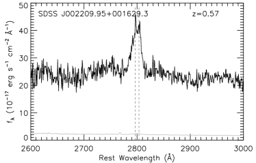
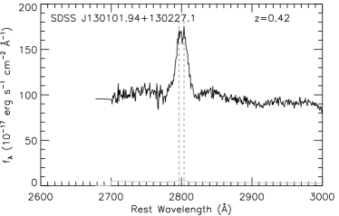
Unlike the cases of H and H, it is somewhat ambiguous whether it is necessary to subtract a narrow line component for MgII and if so, how to do it. On one hand, for some objects, such as SDSSJ002209.95+001629.3 and SDSSJ130101.94+130227.1 (e.g., Fig. 2), the spectral quality is sufficient to see the bifurcation of the MgII doublet around the peak. The locations of the two peaks indicate that they are associated with the MgII 2796,2803 doublet, and the fact that they are resolved means that the FWHM of each component is , hence they are most likely associated with the narrow line region. On the other hand, such cases are rare and most SDSS spectra do not have adequate S/N to unambiguously locate the narrow MgII doublet. Associated narrow MgII absorption troughs can further complicate the situation by mimicing two peaks. Hence although our approach of fitting a single Gaussian to the narrow MgII component is not perfect, it nevertheless accounts for some narrow MgII contamination. Fig. 3 compares our broad MgII FWHM measurements with those from Wang et al. (2009b) for the objects in both studies. Although we have used a different approach, our results are consistent with theirs, with a mean offset dex. This systematic offset between our results and theirs is caused by the fact that they are treating the broad MgII line as a doublet as well, while we (and most studies) are treating the broad MgII line as a single component.

3.4. CIV
For CIV we fit for objects with . Iron emission is generally weak for CIV, and most of our objects do not have the spectral quality sufficient for a reliable iron template subtraction (e.g., Shen et al., 2008b). The power-law continuum fitting windows are: [1445,1465] Å and [1700,1705] Å. We found fitting CIV with iron subtraction does not change the fitted CIV FWHM significantly, but does systematically reduce the CIV EW by dex because the iron flux under the wings of the CIV line is accounted for. At the same time, fitting iron emission increases the uncertainty in the fitted continuum slope and normalization, due to imperfect subtraction of the iron flux. Therefore we report our CIV measurements without the iron template fits, and emphasize that the CIV EWs may be overestimated by dex on average.
The continuum subtracted line emission within [1500,1600] Å was fitted with three Gaussians (e.g., Shen et al., 2008b), and we measure the line FWHM from the model fit. To reduce the effects of noise spikes, we reject any Gaussian component having flux less than of the total model flux when computing the FWHM. However, unlike some attempts in the literature (e.g., Bachev et al., 2004; Baskin & Laor, 2005; Sulentic et al., 2007; Zamfir et al., 2010), we do not subtract a narrow CIV component because: 1) it is still debatable if a strong narrow CIV component exists for most quasars, or if it is feasible to do such a subtraction; 2) existing CIV virial estimators are calibrated using the FWHMs from the entire CIV profile (Vestergaard & Peterson, 2006).
Many CIV lines are affected by narrow or broad absorption features. To reduce the effects of such absorption on the CIV fits, we mask out outliers below the 20-pixel boxcar-smoothed spectrum during our fits (to remedy for narrow absorption features); we also perform a second fit excluding pixels below of the first model fit, and replace the first one if statistically justified (to account for broad absorption features). We found these recipes can alleviate the impact of narrow or moderate absorption features, but the improvement is marginal for objects severely affected by broad absorption.
3.5. Reliability of spectral fits and error estimation
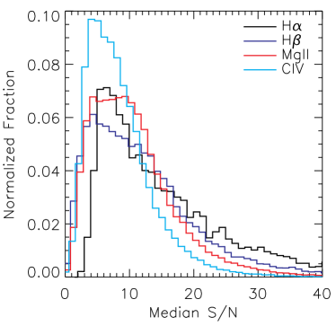
Our spectral fits were performed in an automatic fashion. Upon visual inspection of the fitting results we are confident that the vast majority () of the fits to high S/N spectra were successful, and comparisons with independent fits by others also show good agreement. However, the reliability of our spectral fits drops rapidly for low-quality spectra. Fig. 4 shows the distributions of the median S/N per pixel around the line-fitting region for objects that have line measurements, for H, H, MgII and CIV respectively. Although the bulk of objects have median S/N for the line-fitting regions, there are many objects that have lower median S/N, especially for CIV at high redshift. The effects of S/N on the measurements depend on both the properties of the lines (i.e., line profile, line strength, degree of absorption features, etc), and the line-fitting technique itself (i.e., what functional form was used, how to deal with absorption troughs, etc).
To investigate the impact of S/N on our fitting parameters we ran a series of Monte Carlo simulations. We select representative real spectra with high S/N, then degrade the spectra by adding Gaussian noise and measure the line properties using the same line-fitting routine. For each line (H, MgII, or CIV), we study several objects with various line shapes and EWs. We simulate 500 trials for each S/N level and take the median and the range as the measurement result and its error.
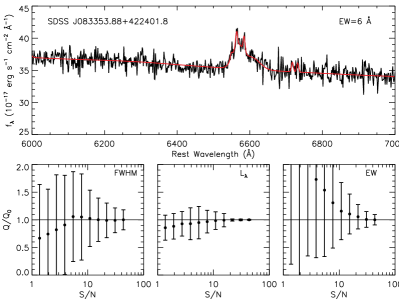
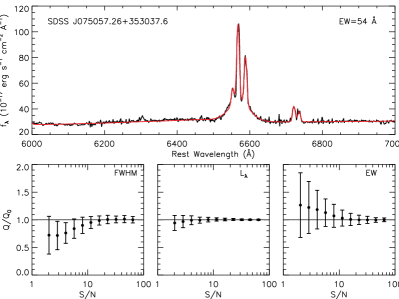
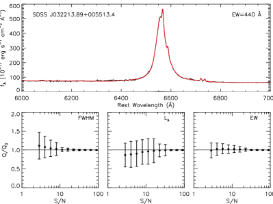
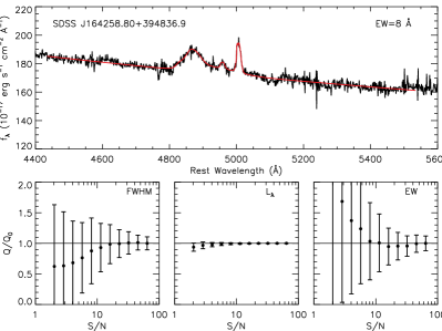
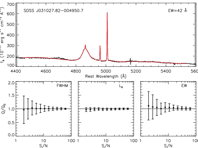
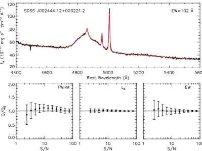
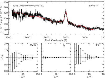
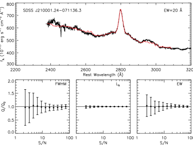
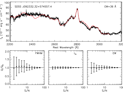
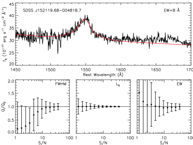
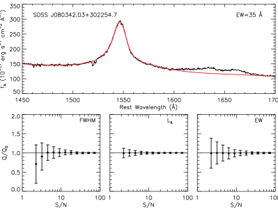
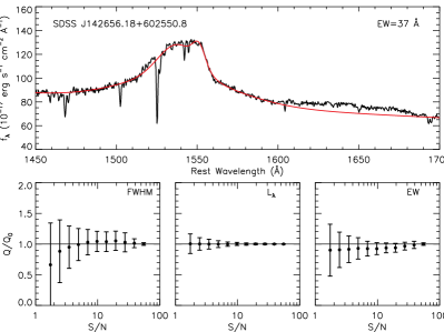
Figs. 5-8 show several examples of our investigations for H, H, MgII and CIV respectively. As expected, decreasing the S/N increases measurement scatter. In all cases the fitted continuum is unbiased as S/N decreases. The FWHMs and EWs are biased by less than for high-EW objects as S/N is reduced to as low as . For low-EW objects, the FWHMs and EWs are biased low/high by for S/N. Since the median EWs for the three lines are Å (see §4.1), we expect that the measurements for most objects are unbiased to within down to S/N. But for many purposes, it would be more conservative to impose a cut at S/N for reliable measurements.
To estimate the uncertainties in the measured quantities in our fits, we generate 50 mock spectra by adding Gaussian noise to the original spectrum using the reported flux density errors, and fit for those mock spectra with the same fitting routines. We estimate the measurement uncertainties from the range (centered on the median) of the distributions of fitting results of the 50 trials. This approach gives more reasonable error estimation than using the statistical errors resulting from the fits, in the sense that it not only takes into account the spectral S/N but also the ambiguity of subtracting a narrow line component in many cases (for H, H and MgII). We estimate the spectral measurement uncertainties for all the 105,783 quasars in our sample in this way.
Given the automatic nature and specifics of our fitting recipe, there will undoubtedly be bad fits for noisy spectra or peculiar objects. We recommend using the reported measurement errors to remove suspicious measurements, e.g., Err AND Err some threshold. Our fitting recipe was optimized for the vast majority of quasars in our sample, and it may fail badly for rare objects with peculiar continuum and emission line properties. These objects include severe BALQSOs, disk emitters, and objects such as J094215.12+090015.8, which has extremely broad lines that exceed our line fitting range. One should pay attention to our fitting ranges and these special objects upon usage of the cataloged quantities. For various reasons, one may want to check the quality assessment (QA) plot for individual fits to make sure that the fitting results are robust. Such QA plots are provided along with this catalog.
Finally, we note that we imposed a FWHM limit of for the narrow line components when fitting H, H and MgII. This choice is motivated by the results in Hao et al. (2005), but is still somewhat arbitrary; narrow lines broader than this threshold are not unusual. On the other hand, if a Gaussian component with FWHM can be fit to H, H and MgII, it will be considered as a narrow line component and subtracted off. For these reasons, we urge caution regarding objects for which the measured narrow line FWHM reaches the limit ( a few percent). Upon visual inspection of the QA plots for these objects, even though the FWHM parameter reaches the limit, most of the fits still yield reasonable measurements of total line flux, line centroid and narrow line subtraction.
3.6. Host galaxy contamination
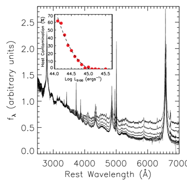
For the vast majority of objects in our catalog with , host galaxy contamination is negligible. However, for the low-luminosity quasars in our sample, the continuum luminosity at restframe Å may be contaminated by light from the host galaxies. Unfortunately the spectral quality of the majority of individual objects does not allow a reliable galaxy continuum subtraction. Here we estimate the effects of host contamination with stacked spectra.
We take all quasars with measurable rest frame Å continuum luminosity, , and bin them on a grid of for . Following Vanden Berk et al. (2001), we generate geometric mean composite spectra for objects in each luminosity bin. The composite spectra are shown in Fig. 9, where the flux gradually flattens at long wavelengths due to increasing host contamination at fainter luminosities. This trend is accompanied by the increasing prominence of stellar absorption features and narrow line emission towards fainter luminosities. The inset shows the fractional host contamination at Å assuming that the highest luminosity bin () is not affected by the host and that the intrinsic AGN power-law continuum slope does not change over the luminosity range considered. The host contamination is substantial at , and becomes negligible towards higher luminosities. The median value of for quasars in this low-redshift sample is , and therefore the host contamination on average is , which leads to a dex overestimation of the Å continuum luminosity and thus dex overestimation of the H-based virial masses for the median object. While we do not correct the measured 5100Å continuum luminosity (and other quantities depending on it) in the catalog, we provide an empirical fitting formula of the average host contamination based on the stacked spectra (dashed line in the inset of Fig. 9):
| (1) |
for ; no correction is needed for luminosities above this value.
3.7. Virial BH masses
It has become common practice to estimate quasar/AGN BH masses based on single-epoch spectra (hereafter virial mass in short). This approach assumes that the broad line region (BLR) is virialized, the continuum luminosity666We note that in a few extremely radio-loud quasars, the continuum luminosity is significantly boosted by the optical emission from the jet, which will then lead to overestimation of the BLR size and the virial BH mass (e.g., Wu et al., 2004). The fraction of such objects in our sample is tiny and hence we neglect this detail. But we caution the usage of cataloged virial BH masses for such objects. is used as a proxy for the BLR radius, and the broad line width (FWHM or line dispersion) is used as a proxy for the virial velocity. The virial mass estimate can be expressed as:
| (2) |
where the coefficients and are empirically calibrated against local AGNs with RM masses or internally among different lines. H, MgII, CIV, and their corresponding continuum luminosities are all frequently adopted in such virial calibrations. Although it is straightforward to calibrate and use these virial estimators, one must bear in mind the large uncertainties ( dex) associated with these estimates and the systematics involved in the calibration and usage, which will potentially lead to significant biases of these BH mass estimates (e.g., Collin et al., 2006; Shen et al., 2008b; Marconi et al., 2008; Denney et al., 2009; Kelly et al., 2009; Shen & Kelly, 2010).
The virial BH mass calibrations used in this paper are from McLure & Dunlop (2004, H and MgII), Vestergaard & Peterson (2006, H and CIV), and Vestergaard & Osmer (2009, MgII). These calibrations have parameters:
| (3) | |||||
| (4) | |||||
| (5) | |||||
| (6) | |||||
| (7) |
In using each of these relations we choose the proper FWHM definition adopted in these calibrations. In order to utilize our new MgII FWHM measurements (e.g., multiple-Gaussian fits with narrow line subtraction, see §3.3), we adopt the slope in the BLR radiusluminosity relation in McLure & Dunlop (2004), and recalibrate the coefficient such that the MgII-based estimates are consistent with the H-based (VP06) estimates on average. We choose this particular slope because it was re-calibrated in McLure & Dunlop (2004) using a subsample of reverberation mapping AGNs that occupy the high-luminosity regime in the local RM AGN sample, arguably better than using the whole RM sample. We choose the VP06 H formula to calibrate our MgII formula because the FWHMs of broad H and MgII were measured in a similar fashion (as opposed to the single-Gaussian or Lorentzian profile adopted in McLure & Dunlop 2004). This new MgII calibration is
| (8) |
In some cases a particular line may be unavailable in the spectrum, or the continuum is too faint to measure. Below we provide several alternative empirical recipes to estimate a virial BH mass. These recipes are calibrated using correlations among continuum and emission line properties, and are only valid in the average sense. We recommend to use them only when the above estimators are unavailable.
Following Greene & Ho (2005b), a virial BH mass can be estimated based on the FWHM and luminosity of the broad H line. We found a correlation between the FWHMs (using multiple-Gaussian fits) of the broad H and H lines similar to that found in previous work (e.g., Greene & Ho, 2005b; Shen et al., 2008a), with the broad H FWHM systematically larger than the broad H FWHM:
| (9) | |||||
where the slope and intercept are determined using the BCES bisector linear regression estimator (e.g., Akritas & Bershady 1996) for a sample of quasars with both H and H FWHM measurements and FWHM errors less than . Our continuum luminosities at 5100 Å have a narrow dynamical range and suffer from host contamination at the low-luminosity end, hence instead of fitting a new relation using our measurements, we adopt the relation between 5100 Å continuum luminosity and H line luminosity in Greene & Ho (2005b, their eqn. 1). The virial mass estimator based on H therefore reads
| (10) | |||||
where is the total H line luminosity. For quasars in our sample, Eqn. (10) yields virial BH masses consistent with the VP06 H results, with a mean offset dex and a dispersion dex.
Similarly, we can substitute the continuum luminosity in the above recipes for H, MgII and CIV with the luminosity of the particular line used, given that for broad line quasars the line luminosity correlates with the continuum luminosity to some extent. We determine these correlations using subsamples of quasars for which both luminosities were measured with an uncertainty dex. For the same reason as H, we do not fit a new relation between the H line luminosity and continuum luminosity at 5100 Å, and we refer to eqn. (2) of Greene & Ho (2005b) for such a relation. The following relations are determined again using the BCES linear regression estimator (for both the bisector fit and the fit, where the latter refers to “predict as a function of ”), where the line luminosity refers to the total line luminosity777For MgII, the difference between the total line luminosity and the broad line luminosity is small enough such that it essentially makes no difference in the linear regression results when we use the broad line luminosity instead.:
where the scatter of this correlation is (0.16) dex for quasars, and
where the scatter of this correlation is (0.2) dex for quasars. Using our measurements, one can also estimate these correlations with other linear regression algorithms. If we substitute and using Eqns. (12) and (14) in the MgII and CIV estimators, we obtain virial BH masses consistent with the original recipes with no mean offset ( dex) and negligible scatter ( dex).


There are systematic differences among different versions of virial calibrations. For instance, the calibrations for H and MgII in McLure & Dunlop (2004) used the old RM masses and virial coefficient, while those in Vestergaard & Peterson (2006) and Vestergaard & Osmer (2009) used the updated RM masses and virial coefficient (Onken et al., 2004). Significant uncertainties of the virial coefficient still remain (e.g., Woo et al., 2010; Graham et al., 2011). Moreover, different versions of virial calibration for the same line have different dependence on luminosity, and they usually measure the line FWHM differently (even though occasionally different approaches to measure the FWHM yield the same value during the multi-parameter fits), or prefer an alternative proxy (e.g., line dispersion) for the virial velocity (e.g., Collin et al., 2006; Rafiee & Hall, 2010). Currently there is no consensus on which version of calibration is better. It is important to explore various systematics with RM AGN samples and statistical quasar samples to determine which is the best approach to estimate quasar BH masses with the virial technique, and this is work in progress (e.g., Onken & Kollmeier, 2008; Denney et al., 2009; Wang et al., 2009b; Rafiee & Hall, 2010). In the mean time, there is strong need to increase the sample size and representativity of AGNs with RM measurements, which anchor these single-epoch virial estimators.
Here we simply settle on a fiducial virial mass estimate: we use H (VP06) estimates for , MgII (S10) estimates for and CIV (VP06) estimates for . Fig. 10 shows the comparison between these virial estimates between two lines for the subset of quasars for which both line estimates are available and the median line S/N. There is negligible mean offset ( dex) between these virial estimates (half by design), which motivated our choice of these three calibrations. However, as noted in Shen et al. (2008b), there is a strong trend of decreasing the ratio of with increasing CIV-MgII blueshifts, indicating a possible non-virialized component in CIV. Richards et al. (2011) further developed a unified picture in which the CIV line has both a non-virial wind component and a traditional virial component, and it is plausible that the BH mass scaling relation based on CIV is only relevant for objects dominated by the virial component.
3.8. The spectral catalog
We have tabulated all the measured quantities from the spectral fitting in the online catalog of this paper, along with other properties888Note that in Shen et al. (2008b) we only reported high-quality measurements with median S/N and a reduced for a single-Gaussian fit to the line; here we retain all measurements for completeness.. The current compilation extends our earlier SDSS Data Release 5 (DR5) compilation (Shen et al., 2008b) by including the post-DR5 quasars, as well as measurements based on new multiple-Gaussian fits to the lines (as discussed above). The format of the catalog is described in Table 1. Objects are in the same order as the DR7 quasar catalog in Schneider et al. (2010). Below we describe the specifics of the cataloged quantities. The SDSS terminology can be found on the SDSS website999http://www.sdss.org/dr7/. Flux measurements were corrected neither for intrinsic extinction/reddening, nor for host contamination. We only report FWHM and velocity shift values for detectable line components (i.e., the fitted line flux is non-zero), except for cases where the line FWHM and velocity offset can be inferred from other lines (such as the narrow H line, whose FWHM and velocity offset are tied to those of the [O III] doublet).
-
1.
SDSS DR7 designation: hhmmss.ss+ddmmss.s (J2000.0; truncated coordinates)
-
2-4.
RA and DEC (in decimal degrees, J2000.0), redshift. Here the redshifts are taken from the DR7 quasar catalog (Schneider et al., 2010). Hewett & Wild (2010) provided improved redshifts for SDSS quasars. These improved redshifts are particularly useful for generating coadded spectra, but the cataloged DR7 redshifts are fine for most of the purposes considered here.
-
5-7.
Spectroscopic plate, fiber and Modified Julian date (MJD): the combination of plate-fiber-MJD locates a particular spectroscopic observation in SDSS. The same object can be observed more than once with different plate-fiber-MJD combinations either on a repeated plate (same plate and fiber numbers but different MJD number), or on different plates. The DR7 quasar catalog typically lists the spectroscopic observation with the highest S/N.
-
8.
TARGET_FLAG_TARGET: the target selection flag (TARGET version).
-
9.
: number of spectroscopic observations. While we only used the default spectrum in our spectral fitting, this flag indicates if there are multiple spectroscopic observations for each object.
-
10.
Uniform flag. 0=not in the uniform sample101010For more details regarding the uniform sample selection and its sky coverage, see, e.g., Richards et al. (2002a, 2006b); Shen et al. (2007).; 1=uniformly selected using the target selection algorithm in Richards et al. (2002a), and flux limited to at or at ; 2=selected by the QSO_HiZ branch only in the uniform target selection (Richards et al., 2002a) and with measured spectroscopic redshift and . Objects with uniform flag=2 are selected by the uniform quasar target algorithm, but should not be included in statistical studies; the fraction of such uniform objects is low (; red dots in Fig. 1).
-
11.
: absolute -band magnitude in the current cosmology, -corrected to following111111The -corrections here include both continuum -correction and emission-line -correction (Richards et al., 2006b); while the cataloged absolute magnitudes in Schneider et al. (2010) were -corrected for continuum only, assuming a power-law continuum. Richards et al. (2006b).
-
12-13.
Bolometric luminosity and its error: computed from (), (), () using the spectral fits and bolometric corrections121212The SEDs for individual quasars show significant scatter (e.g., Richards et al., 2006a), so the adopted bolometric corrections are only appropriate in the average sense. Some authors suggest to remove the IR bump in the SED in estimating the bolometric corrections (e.g., Marconi et al., 2004), where the IR radiation is assumed to come from the reprocessed UV radiation. This will generally reduce the bolometric corrections by about one third. However, we are not correcting for intrinsic extinction of the flux, and we did not subtract emission line flux in the Richards et al. composite SED when estimating the bolometric corrections, hence using our fiducial bolometric corrections will not overestimate the bolometric luminosity significantly. , and from the composite SED in Richards et al. (2006a).
-
14.
BAL flag: 0=nonBALQSO or no wavelength coverage; 1=CIV HiBALQSO; 2=MgII LoBALQSO; 3=both 1 and 2. The LoBALQSO selection is very incomplete as discussed in §2.
- 15.
-
16-17.
Observed radio flux density at rest-frame cm and optical flux density at rest-frame Å . Both are in the observed frame.
-
18.
Radio loudness .
-
19-24.
, , and their errors: continuum luminosity at Å, Å and Å, measured from the spectral fits. No correction for host contamination is made (see discussion in §3.6).
-
25-30.
Line luminosity, FWHM, restframe equivalent width and their errors for the broad H component.
-
31-36.
Line luminosity, FWHM, restframe equivalent width and their errors for the narrow H component.
-
37-40.
Line luminosity, restframe equivalent width and their errors for narrow [N II] 6584.
-
41-44.
Line luminosity, restframe equivalent width and their errors for narrow [S II] 6717.
-
45-48.
Line luminosity, restframe equivalent width and their errors for narrow [S II] 6731.
-
49-50.
6000-6500 Å iron restframe equivalent width and its error.
-
51-52.
Power-law slope and its error for the continuum fit for H.
-
53-54.
Number of good pixels and median per pixel for the H region (6400-6765 Å).
-
55.
Reduced for the H line fit; if not fitted.
-
56-61.
Line luminosity, FWHM, restframe equivalent width and their errors for the broad H component.
-
62-67.
Line luminosity, FWHM, restframe equivalent width and their errors for the narrow H component.
-
68.
FWHM of broad H using a single Gaussian fit (Shen et al., 2008b).
-
69-72.
Line luminosity, restframe equivalent width and their errors for [O III] 4959.
-
73-76.
Line luminosity, restframe equivalent width and their errors for [O III] 5007.
-
77-78.
4435-4685 Å iron restframe equivalent width and its error.
-
79-80.
Power-law slope and its error for the continuum fit for H.
-
81-82.
Number of good pixels and median per pixel for the H region (4750-4950 Å).
-
83.
Reduced for the H line fit; if not fitted.
-
84-89.
Line luminosity, FWHM, restframe equivalent width and their errors for the whole MgII profile.
-
90-95.
Line luminosity, FWHM, restframe equivalent width and their errors for the broad MgII profile.
-
96.
FWHM of broad MgII using a single Gaussian fit (Shen et al., 2008b).
-
97-98.
2200-3090 Å iron restframe equivalent width and its error.
-
99-100.
Power-law slope and its error for the continuum fit for MgII.
-
101-102.
Number of good pixels and median per pixel for the MgII region (2700-2900 Å).
-
103.
Reduced for the MgII line fit; if not fitted.
-
104-109.
Line luminosity, FWHM, restframe equivalent width and their errors for the whole CIV profile.
-
110-111.
Power-law slope and its error for the continuum fit for CIV.
-
112-113.
Number of good pixels and median per pixel for the CIV region (1500-1600 Å).
-
114.
Reduced for the CIV line fit; if not fitted.
-
115-126.
Velocity shifts (and their errors) relative to the systemic redshift (cataloged in Schneider et al., 2010) for broad H, narrow H, broad H, narrow H, broad MgII, and CIV. The velocity shifts for the broad lines are measured from the peak of the multiple-Gaussian model fit to the broad component131313The velocity shifts of the broad lines measured from the centroid of a single Gaussian fit to the line on average are consistent with those using the peak of the multiple-Gaussian fit with negligible mean offset, but they can differ (typically by ) for individual objects.. Recall that the velocity shifts of narrow lines were tied together during spectral fits. These velocity shifts can be used to compute the relative velocity offsets between two lines for the same object, such as the CIV-MgII blueshift, but should not be interpreted as the velocity shifts from the restframe of the host galaxy due to uncertainties in the systemic redshift. Positive values indicate blueshift and negative values indicate redshift; value of indicates an unmeasurable quantity.
-
127-138.
Virial BH masses using calibrations of H (MD04), H (VP06), MgII (MD04), MgII (VO09), MgII (S10) and CIV (VP06). The definitions of the acronym names of each calibration can be found in §3.7. Zero value indicates an unmeasurable quantity. We use FWHMs from a single Gaussian fit to the broad component for H (MD04) and MgII (MD04); FWHMs from the multiple-Gaussian fit to the broad H for H (VP06); FWHMs from the multiple-Gaussian fit to the entire MgII and CIV lines for MgII (VO09) and CIV (VP06) respectively; FWHMs from the multiple-Gaussian fit to the broad MgII line for MgII (S10). See §3 for details.
-
139.
The adopted fiducial virial BH mass if more than one estimate is available. See detailed discussion in §3.7.
-
140.
The measurement uncertainty of the adopted fiducial virial BH mass, propagated from the measurement uncertainties of continuum luminosity and FWHM. Note that this uncertainty includes neither the statistical uncertainty ( dex) from virial mass calibrations, nor the systematic uncertainties with these virial BH masses.
-
141.
Eddington ratio computed using the fiducial virial BH mass.
-
142.
Special interest flag. This is a binary flag: bit#0 set=disk emitters with high confidence (the vast majority are selected based on the Balmer lines); bit#1 set=disk emitter candidates; bit#2 set=double-peaked [O III] 4959,5007 lines. These flags were set upon visual inspection of all quasars in the catalog. In particular, disk emitter candidates (bit#1=1) are those with asymmetric broad Balmer line profile or systematic velocity shifts from the narrow lines; while those with high confidence (bit#0=1) show unambiguous double-peaked (or highly asymmetric) broad line profile or large velocity offsets between the broad and narrow lines. Fig. 11 shows two examples of disk emitters with high confidence. We call these objects “disk emitters” even though some of them may be explained by alternative scenarios, such as a close SMBH binary (e.g., see discussion in Shen & Loeb, 2010).


4. Applications
The spectral measurements described above can be used to study the statistical properties of broad line quasars. Here we briefly discuss some applications of this spectral catalog.


4.1. Correlations between emission line properties
One great virtue of the SDSS DR7 quasar survey is that it provides unprecedented statistics for broad-line quasar properties. To demonstrate this, Figs. 12-14 show some statistical properties of quasars using our spectral measurements for H, MgII, and CIV, respectively. These figures show the typical values of these properties for SDSS quasars as a quick reference. We do not show a similar figure for H because quasars with H coverage represent only a tiny fraction of the whole sample, and because host contamination is more severe for these low-redshift quasars.
There are correlations among the properties shown in Figs. 12-14. Some of these correlations are not due to selection effects. For instance, the well-known Baldwin effect (Baldwin, 1977), i.e., the anti-correlation between line EW and continuum luminosity, is clearly seen for CIV and MgII. There are also strong correlations between EW and FWHM for MgII (e.g., Dong et al., 2009b) and CIV, which are not due to any apparent selection effects. The statistics of our catalog now allows in-depth investigations of these correlations when binning in different quantities such as redshift or luminosity, and to probe the origins of these correlations. However, there are some apparent correlations which are likely due to selection effects inherent in a flux-limited sample, or host contamination. For instance, the apparent anti-correlation between and , and the mild negative Baldwin effect below for H seen in Fig. 12, are most likely caused by increasing host contamination towards fainter luminosities (see §3.6). Moreover, the spectral quality (mainly S/N) has important effects on the measured quantities and may bias the measurements at the low S/N end. Thus one must take these issues into account when using the catalog to study correlations among various properties. The detailed investigations of various correlations will be presented elsewhere.

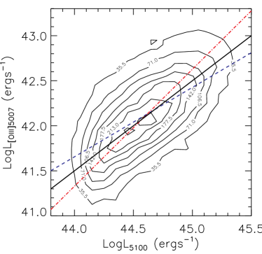
Fig. 15 shows the so-called 4DE1 projection in the H FWHM versus space (e.g., Sulentic et al., 2000, 2002; Zamfir et al., 2010), which is an extension of the eigenvector space for quasar properties suggested by Boroson & Green (1992). Objects with H FWHM (i.e., population “B” in the terminology of the 4DE1 parameter space of Sulentic and collaborators) have a tendency to have weaker relative iron emission strength for larger FWHMs. The black contours show the distribution of all quasars while the red contours show the distribution of radio-loud () quasars. It appears that the radio-loud contours are more vertically elongated, broadly consistent with the phenomenological classification scheme based on the 4DE1 parameter space (e.g., Sulentic et al., 2000, 2002; Zamfir et al., 2010). The physics driving these characteristics in the parameter space is currently not clear, and deserves further study.
Fig. 16 shows the correlation between the [O III] 5007 luminosity and the continuum luminosity at Å. This correlation is usually used to estimate the bolometric luminosity using the [O III] 5007 luminosity as a surrogate for type 2 quasars (e.g, Kauffmann et al., 2003; Zakamska et al., 2003; Heckman et al., 2004; Reyes et al., 2008). While the correlation is apparent, it has a large scatter, as noted in earlier studies (e.g., Heckman et al., 2004; Reyes et al., 2008). The mean linear relation is:
| (15) |
with a scatter dex. Using the bolometric correction from Richards et al. (2006a), a crude conversion between and the quasar bolometric luminosity is: .
4.2. Emission line shifts
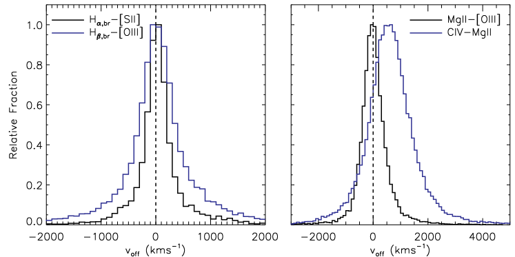
Fig. 17 shows the distributions of velocity shifts between various emission lines. Recall that the velocity of the broad lines is measured from the peak of the multiple-Gaussian fit. The left panel of Fig. 17 shows the distributions of velocity shifts between the broad Balmer lines and the narrow lines. The means of these distributions are consistent with zero, hence there is no offset in the mean between the broad and narrow Balmer lines (cf., Bonning et al., 2007). We note that if we did not account for the blue wings of the narrow [O III] 4959,5007 lines during spectral fitting, there would be a net redshift of the order of between the broad H line and [O III], which is inconsistent with the results for H versus [S II]. The right panel of Fig. 17 shows the velocity offsets between MgII and [O III] and between CIV and MgII. The MgII line shows no mean offset from [O III], while the CIV line shows a systematic blueshift of with respect to MgII (e.g., Gaskell, 1982; Tytler & Fan, 1992; Richards et al., 2002b); see Richards et al. (2011) for further discussion.
It is interesting to note that many of the objects in the wings of the velocity offset distributions of the broad Balmer lines vs the narrow lines are either strong disk-emitters (e.g., Chen et al., 1989; Eracleous & Halpern, 1994; Strateva et al., 2003), or have the broad component systematically offset from the narrow line center; in other cases the apparent large shifts were caused by poor fits to noisy spectra.
5. Summary
We have constructed an SDSS DR7 quasar catalog in which we tabulate various properties. In this catalog we compiled continuum and emission line properties for H, H, MgII, and CIV based on our spectral fits. We also included radio properties, and flagged quasars of special interest, such as broad absorption line quasars and disk emitters. We also compiled virial BH mass estimates using these spectral measurements. This catalog can be used to study correlations among properties of optically selected quasars, and the active black hole mass function in quasars (Shen et al., in preparation). We performed various tests and found that our automatic fitting procedure to emission lines performed reasonably well. However, one must take into account the possible effects of selection and S/N, as well as the systematics involved in converting the measured quantities to derived quantities, when using these measurements to study quasar properties. In particular, we do not encourage direct interpretations based on derived quantities (such as virial BH masses and bolometric luminosity) without accounting for the difference between the estimated value and the true value for these quantities. Such direct interpretations will usually lead to biased or even spurious results.
We make this catalog publicly available online141414 http://www.cfa.harvard.edu/yshen/BH_mass/dr7.htm, where we also provide supplemental materials (such as dereddened spectra, QA plots, etc) and important future updates of this compilation.
References
- Abazajian et al. (2009) Abazajian, K. N., et al. 2009, ApJS, 182, 543
- Adelman-McCarthy et al. (2008) Adelman-McCarthy, J. K., et al. 2008, ApJS, 175, 297
- Akritas & Bershady (1996) Akritas, M. G., & Bershady, M. A. 1996, ApJ, 470, 706
- Bachev et al. (2004) Bachev, R., Marziani, P., Sulentic, J. W., Zamanov, R., Calvani, M., & Dultzin-Hacyan, D. 2004, ApJ, 617, 171
- Baldwin (1977) Baldwin, J. A. 1977, ApJ, 214, 679
- Baskin & Laor (2005) Baskin, A., & Laor, A. 2005, MNRAS, 356, 1029
- Blanton et al. (2003) Blanton, M. R., Lin, H., Lupton, R. H., Maley, F. M., Young, N., Zehavi, I., & Loveday, J. 2003, AJ, 125, 2276
- Bonning et al. (2007) Bonning, E. W., Shields, G. A., & Salviander, S. 2007, ApJ, 666, L13
- Boroson & Green (1992) Boroson, T. A., & Green, R. F. 1992, ApJS, 80, 109
- Cardelli et al. (1989) Cardelli, J. A., Clayton, G. C., & Mathis, J. S. 1989, ApJ, 345, 245
- Chen et al. (1989) Chen, K., Halpern, J. P., & Filippenko, A. V. 1989, ApJ, 339, 742
- Collin et al. (2006) Collin, S., Kawaguchi, T., Peterson, B. M., & Vestergaard, M. 2006, A&A, 456, 75
- Croom et al. (2002) Croom, S. M., et al. 2002, MNRAS, 337, 275
- Croom et al. (2004) Croom, S. M., Smith, R. J., Boyle, B. J., Shanks, T., Miller, L., Outram, P. J., & Loaring, N. S. 2004, MNRAS, 349, 1397
- Denney et al. (2009) Denney, K. D., et al. 2009, ApJ, 704, L80
- Dietrich & Hamann (2004) Dietrich, M., & Hamann, F. 2004, ApJ, 611, 761
- Dong et al. (2009a) Dong, X., Wang, J., Wang, T., Wang, H., Fan, X., Zhou, H., & Yuan, W. 2009a, ArXiv e-prints
- Dong et al. (2009b) Dong, X., Wang, T., Wang, J., Fan, X., Wang, H., Zhou, H., & Yuan, W. 2009b, ApJ, 703, L1
- Eracleous & Halpern (1994) Eracleous, M., & Halpern, J. P. 1994, ApJS, 90, 1
- Fine et al. (2008) Fine, S., et al. 2008, MNRAS, 390, 1413
- Fine et al. (2006) —. 2006, MNRAS, 373, 613
- Fukugita et al. (1996) Fukugita, M., Ichikawa, T., Gunn, J. E., Doi, M., Shimasaku, K., & Schneider, D. P. 1996, AJ, 111, 1748
- Gaskell (1982) Gaskell, C. M. 1982, ApJ, 263, 79
- Gaskell (2010) Gaskell, C. M. 2010, Nature, 463, 1
- Gibson et al. (2009) Gibson, R. R., et al. 2009, ApJ, 692, 758
- Graham et al. (2011) Graham, A. W., Onken, C. A., Athanassoula, E., & Combes, F. 2011, MNRAS, in press, arXiv:1007.3834
- Greene & Ho (2005a) Greene, J. E., & Ho, L. C. 2005a, ApJ, 627, 721
- Greene & Ho (2005b) —. 2005b, ApJ, 630, 122
- Gunn et al. (1998) Gunn, J. E., et al. 1998, AJ, 116, 3040
- Gunn et al. (2006) —. 2006, AJ, 131, 2332
- Hao et al. (2005) Hao, L., et al. 2005, AJ, 129, 1783
- Heckman et al. (1981) Heckman, T. M., Miley, G. K., van Breugel, W. J. M., & Butcher, H. R. 1981, ApJ, 247, 403
- Heckman et al. (2004) Heckman, T. M., Kauffmann, G., Brinchmann, J., Charlot, S., Tremonti, C., & White, S. D. M. 2004, ApJ, 613, 109
- Hewett & Wild (2010) Hewett, P. C. & Wild, V. 2010, MNRAS, 405, 2302
- Hogg et al. (2001) Hogg, D. W., Finkbeiner, D. P., Schlegel, D. J., & Gunn, J. E. 2001, AJ, 122, 2129
- Hopkins et al. (2006) Hopkins, P. F., Hernquist, L., Cox, T. J., Di Matteo, T., Robertson, B., & Springel, V. 2006, ApJS, 163, 1
- Hopkins et al. (2008) Hopkins, P. F., Hernquist, L., Cox, T. J., & Kereš, D. 2008, ApJS, 175, 356
- Hu et al. (2008a) Hu, C., Wang, J., Ho, L. C., Chen, Y., Bian, W., & Xue, S. 2008a, ApJ, 683, L115
- Hu et al. (2008b) Hu, C., Wang, J., Ho, L. C., Chen, Y., Zhang, H., Bian, W., & Xue, S. 2008b, ApJ, 687, 78
- Ivezić et al. (2004) Ivezić, Ž., et al. 2004, Astronomische Nachrichten, 325, 583
- Jiang et al. (2007) Jiang, L., Fan, X., Ivezić, Ž., Richards, G. T., Schneider, D. P., Strauss, M. A., & Kelly, B. C. 2007, ApJ, 656, 680
- Kauffmann & Haehnelt (2000) Kauffmann, G., & Haehnelt, M. 2000, MNRAS, 311, 576
- Kauffmann et al. (2003) Kauffmann, G., et al. 2003, MNRAS, 341, 33
- Kelly et al. (2009) Kelly, B. C., Vestergaard, M., & Fan, X. 2009, ApJ, 692, 1388
- Kollmeier et al. (2006) Kollmeier, J. A., et al. 2006, ApJ, 648, 128
- Komossa et al. (2008) Komossa, S., Xu, D., Zhou, H., Storchi-Bergmann, T., & Binette, L. 2008, ApJ, 680, 926
- Lin et al. (2010) Lin, Y.-T., Shen, Y., Strauss, M. A., Richards, G. T., & Lunnan, R. 2010, ApJ, 723, 1119
- Liu et al. (2010a) Liu, X., Shen, Y., Strauss, M. A., & Greene, J. E. 2010a, ApJ, 708, 427
- Liu et al. (2010b) Liu, X., Greene, J. E., Shen, Y., & Strauss, M. A. 2010b, ApJ, 715, L30
- Lupton et al. (2001) Lupton, R., Gunn, J. E., Ivezić, Z., Knapp, G. R., & Kent, S. 2001, in Astronomical Society of the Pacific Conference Series, Vol. 238, Astronomical Data Analysis Software and Systems X, ed. F. R. Harnden, Jr., F. A. Primini, & H. E. Payne, 269
- Marconi et al. (2008) Marconi, A., Axon, D. J., Maiolino, R., Nagao, T., Pastorini, G., Pietrini, P., Robinson, A., & Torricelli, G. 2008, ApJ, 678, 693
- Marconi et al. (2004) Marconi, A., Risaliti, G., Gilli, R., Hunt, L. K., Maiolino, R., & Salvati, M. 2004, MNRAS, 351, 169
- Marziani et al. (1996) Marziani, P., Sulentic, J. W., Dultzin-Hacyan, D., Calvani, M., & Moles, M. 1996, ApJS, 104, 37
- McGill et al. (2008) McGill, K. L., Woo, J., Treu, T., & Malkan, M. A. 2008, ApJ, 673, 703
- McLure & Dunlop (2004) McLure, R. J., & Dunlop, J. S. 2004, MNRAS, 352, 1390 (MD04)
- McLure & Jarvis (2002) McLure, R. J., & Jarvis, M. J. 2002, MNRAS, 337, 109
- Onken et al. (2004) Onken, C. A., Ferrarese, L., Merritt, D., Peterson, B. M., Pogge, R. W., Vestergaard, M., & Wandel, A. 2004, ApJ, 615, 645
- Onken & Kollmeier (2008) Onken, C. A., & Kollmeier, J. A. 2008, ApJ, 689, L13
- Pier et al. (2003) Pier, J. R., Munn, J. A., Hindsley, R. B., Hennessy, G. S., Kent, S. M., Lupton, R. H., & Ivezić, Ž. 2003, AJ, 125, 1559
- Rafiee & Hall (2010) Rafiee, A., & Hall, P. B. 2010, ApJS, submitted
- Reyes et al. (2008) Reyes, R., et al. 2008, AJ, 136, 2373
- Richards et al. (2002a) Richards, G. T., et al. 2002a, AJ, 123, 2945
- Richards et al. (2006a) —. 2006a, ApJS, 166, 470
- Richards et al. (2006b) —. 2006b, AJ, 131, 2766
- Richards et al. (2002b) Richards, G. T., Vanden Berk, D. E., Reichard, T. A., Hall, P. B., Schneider, D. P., SubbaRao, M., Thakar, A. R., & York, D. G. 2002b, AJ, 124, 1
- Richards et al. (2011) Richards, G. T., et al. 2011, AJ, 141, 167
- Salviander et al. (2007) Salviander, S., Shields, G. A., Gebhardt, K., & Bonning, E. W. 2007, ApJ, 662, 131
- Schlegel et al. (1998) Schlegel, D. J., Finkbeiner, D. P., & Davis, M. 1998, ApJ, 500, 525
- Schneider et al. (2007) Schneider, D. P., et al. 2007, AJ, 134, 102
- Schneider et al. (2010) —. 2010, AJ, 139, 2360
- Shankar et al. (2009) Shankar, F., Weinberg, D. H., & Miralda-Escudé, J. 2009, ApJ, 690, 20
- Shen et al. (2008a) Shen, J., Vanden Berk, D. E., Schneider, D. P., & Hall, P. B. 2008a, AJ, 135, 928
- Shen (2009) Shen, Y. 2009, ApJ, 704, 89
- Shen et al. (2008b) Shen, Y., Greene, J. E., Strauss, M. A., Richards, G. T., & Schneider, D. P. 2008b, ApJ, 680, 169
- Shen et al. (2011) Shen, Y., Liu, X., Greene, J. E., & Strauss, M. A. 2011, ApJ, submitted, arXiv:1011.5246
- Shen & Kelly (2010) Shen, Y., & Kelly, B. C. 2010, ApJ, 713, 41
- Shen & Loeb (2010) Shen, Y., & Loeb, A. 2010, ApJ, 725, 249
- Shen et al. (2007) Shen, Y., et al. 2007, AJ, 133, 2222
- Smith et al. (2002) Smith, J. A., et al. 2002, AJ, 123, 2121
- Smith et al. (2009) Smith, K. L., Shields, G. A., Bonning, E. W., McMullen, C. C., & Salviander, S. 2010, 716, 866
- Stoughton et al. (2002) Stoughton, C., et al. 2002, AJ, 123, 485
- Strateva et al. (2003) Strateva, I. V., et al. 2003, AJ, 126, 1720
- Sulentic et al. (2007) Sulentic, J. W., Bachev, R., Marziani, P., Negrete, C. A., & Dultzin, D. 2007, ApJ, 666, 757
- Sulentic et al. (2002) Sulentic, J. W., Marziani, P., Zamanov, R., Bachev, R., Calvani, M., & Dultzin-Hacyan, D. 2002, ApJ, 566, L71
- Sulentic et al. (2000) Sulentic, J. W., Zwitter, T., Marziani, P., & Dultzin-Hacyan, D. 2000, ApJ, 536, L5
- Tucker et al. (2006) Tucker, D. L., et al. 2006, Astronomische Nachrichten, 327, 821
- Tytler & Fan (1992) Tytler, D., & Fan, X. 1992, ApJS, 79, 1
- van der Marel & Franx (1993) van der Marel, R. P., & Franx, M. 1993, ApJ, 407, 525
- Vanden Berk et al. (2001) Vanden Berk, D. E., et al. 2001, AJ, 122, 549
- Vestergaard (2002) Vestergaard, M. 2002, ApJ, 571, 733
- Vestergaard & Osmer (2009) Vestergaard, M., & Osmer, P. S. 2009, ApJ, 699, 800 (VO09)
- Vestergaard & Peterson (2006) Vestergaard, M., & Peterson, B. M. 2006, ApJ, 641, 689 (VP06)
- Vestergaard & Wilkes (2001) Vestergaard, M., & Wilkes, B. J. 2001, ApJS, 134, 1
- Wang et al. (2009a) Wang, J., Chen, Y., Hu, C., Mao, W., Zhang, S., & Bian, W. 2009a, ApJ, 705, L76
- Wang et al. (2009b) Wang, J., et al. 2009b, ApJ, 707, 1334
- White et al. (1997) White, R. L., Becker, R. H., Helfand, D. J., & Gregg, M. D. 1997, ApJ, 475, 479
- Woo et al. (2010) Woo, J.-H., et al. 2010, ApJ, 716, 269
- Wu et al. (2004) Wu, X.-B., Wang, R., Kong, M. Z., Liu, F. K, & Han, J. L. 2004, A&A, 424, 793
- Wu et al. (2009) Wu, J., Vanden Berk, D. E., Brandt, W. N., Schneider, D. P., Gibson, R. R., & Wu, J. 2009, ApJ, 702, 767
- Wyithe & Loeb (2003) Wyithe, J. S. B., & Loeb, A. 2003, ApJ, 595, 614
- York et al. (2000) York, D. G., et al. 2000, AJ, 120, 1579
- Zakamska et al. (2003) Zakamska, N. L., et al. 2003, AJ, 126, 2125
- Zamfir et al. (2010) Zamfir, S., Sulentic, J. W., Marziani, P., & Dultzin, D. 2010, MNRAS, 403, 1759
| Column | Format | Description |
|---|---|---|
| 1 | STRING | SDSS DR7 designation hhmmss.ssddmmss.s (J2000.0) |
| 2 | DOUBLE | Right ascension in decimal degrees (J2000.0) |
| 3 | DOUBLE | Declination in decimal degrees (J2000.0) |
| 4 | DOUBLE | Redshift |
| 5 | LONG | Spectroscopic plate number |
| 6 | LONG | Spectroscopic fiber number |
| 7 | LONG | MJD of spectroscopic observation |
| 8 | LONG | Target selection flag (TARGET version) |
| 9 | LONG | Number of spectroscopic observations |
| 10 | LONG | Uniform selection flag |
| 11 | DOUBLE | [, , , -corrected to , following Richards et al. (2006b)] |
| 12 | DOUBLE | Bolometric luminosity [] |
| 13 | DOUBLE | Uncertainty in |
| 14 | LONG | BAL flag (0=nonBALQSO or no wavelength coverage; 1=CIV BALQSO; 2=MgII BALQSO; 3=both 1 and 2) |
| 15 | LONG | FIRST radio flag (-1=not in FIRST footprint; 0=FIRST undetected; 1=core-dominant; 2=lobe-dominant) |
| 16 | DOUBLE | Observed radio flux density at rest-frame 6 cm [mJy] |
| 17 | DOUBLE | Observed optical flux density at rest-frame 2500Å [] |
| 18 | DOUBLE | Radio loudness |
| 19 | DOUBLE | Monochromatic luminosity at 5100Å [] |
| 20 | DOUBLE | Uncertainty in |
| 21 | DOUBLE | Monochromatic luminosity at 3000Å [] |
| 22 | DOUBLE | Uncertainty in |
| 23 | DOUBLE | Monochromatic luminosity at 1350Å [] |
| 24 | DOUBLE | Uncertainty in |
| 25 | DOUBLE | Line luminosity of broad H [] |
| 26 | DOUBLE | Uncertainty in |
| 27 | DOUBLE | FWHM of broad H () |
| 28 | DOUBLE | Uncertainty in the broad H FWHM |
| 29 | DOUBLE | Restframe equivalent width of broad H (Å) |
| 30 | DOUBLE | Uncertainty in |
| 31 | DOUBLE | Line luminosity of narrow H [] |
| 32 | DOUBLE | Uncertainty in |
| 33 | DOUBLE | FWHM of narrow H () |
| 34 | DOUBLE | Uncertainty in the narrow H FWHM |
| 35 | DOUBLE | Restframe equivalent width of narrow H (Å) |
| 36 | DOUBLE | Uncertainty in |
| 37 | DOUBLE | Line luminosity of [N II] 6584 [] |
| 38 | DOUBLE | Uncertainty in |
| 39 | DOUBLE | Restframe equivalent width of [N II] 6584 (Å) |
| 40 | DOUBLE | Uncertainty in |
| 41 | DOUBLE | Line luminosity of [S II] 6717 [] |
| 42 | DOUBLE | Uncertainty in |
| 43 | DOUBLE | Restframe equivalent width of [S II] 6717 (Å) |
| 44 | DOUBLE | Uncertainty in |
| 45 | DOUBLE | Line luminosity of [S II] 6731 [] |
| 46 | DOUBLE | Uncertainty in |
| 47 | DOUBLE | Restframe equivalent width of [S II] 6731 (Å) |
| 48 | DOUBLE | Uncertainty in |
| 49 | DOUBLE | Restframe equivalent width of Fe within 6000-6500Å (Å) |
| 50 | DOUBLE | Uncertainty in |
| 51 | DOUBLE | Power-law slope for the continuum fit for H |
| 52 | DOUBLE | Uncertainty in |
| 53 | LONG | Number of good pixels for the restframe 6400-6765Å region |
| 54 | DOUBLE | Median S/N per pixel for the restframe 6400-6765Å region |
| 55 | DOUBLE | Reduced for the H line fit; -1 if not fitted |
| 56 | DOUBLE | Line luminosity of broad H [] |
| 57 | DOUBLE | Uncertainty in |
| 58 | DOUBLE | FWHM of broad H () |
| 59 | DOUBLE | Uncertainty in the broad H FWHM |
| 60 | DOUBLE | Restframe equivalent width of broad H (Å) |
| 61 | DOUBLE | Uncertainty in |
| 62 | DOUBLE | Line luminosity of narrow H [] |
| 63 | DOUBLE | Uncertainty in |
| 64 | DOUBLE | FWHM of narrow H () |
| 65 | DOUBLE | Uncertainty in the narrow H FWHM |
| 66 | DOUBLE | Restframe equivalent width of narrow H (Å) |
| 67 | DOUBLE | Uncertainty in |
| 68 | DOUBLE | FWHM of broad H using a single Gaussian fit () |
| 69 | DOUBLE | Line luminosity of [O III] 4959 [] |
| 70 | DOUBLE | Uncertainty in |
| 71 | DOUBLE | Restframe equivalent width of [O III] 4959 (Å) |
| 72 | DOUBLE | Uncertainty in |
| 73 | DOUBLE | Line luminosity of [O III] 5007 [] |
| 74 | DOUBLE | Uncertainty in |
| 75 | DOUBLE | Restframe equivalent width of [O III] 5007 (Å) |
| 76 | DOUBLE | Uncertainty in |
| 77 | DOUBLE | Restframe equivalent width of Fe within 4435-4685Å (Å) |
| 78 | DOUBLE | Uncertainty in |
| 79 | DOUBLE | Power-law slope for the continuum fit for H |
| 80 | DOUBLE | Uncertainty in |
| 81 | LONG | Number of good pixels for the restframe 4750-4950Å region |
| 82 | DOUBLE | Median S/N per pixel for the restframe 4750-4950Å region |
| 83 | DOUBLE | Reduced for the H line fit; -1 if not fitted |
| 84 | DOUBLE | Line luminosity of the whole MgII [] |
| 85 | DOUBLE | Uncertainty in |
| 86 | DOUBLE | FWHM of the whole MgII () |
| 87 | DOUBLE | Uncertainty in the whole MgII FWHM |
| 88 | DOUBLE | Restframe equivalent width of the whole MgII (Å) |
| 89 | DOUBLE | Uncertainty in |
| 90 | DOUBLE | Line luminosity of broad MgII [] |
| 91 | DOUBLE | Uncertainty in |
| 92 | DOUBLE | FWHM of broad MgII () |
| 93 | DOUBLE | Uncertainty in the broad MgII FWHM |
| 94 | DOUBLE | Restframe equivalent width of broad MgII (Å) |
| 95 | DOUBLE | Uncertainty in |
| 96 | DOUBLE | FWHM of broad MgII using a single Gaussian fit () |
| 97 | DOUBLE | Restframe equivalent width of Fe within 2200-3090Å (Å) |
| 98 | DOUBLE | Uncertainty in |
| 99 | DOUBLE | Power-law slope for the continuum fit for MgII |
| 100 | DOUBLE | Uncertainty in |
| 101 | LONG | Number of good pixels for the restframe 2700-2900Å region |
| 102 | DOUBLE | Median S/N per pixel for the restframe 2700-2900Å region |
| 103 | DOUBLE | Reduced for the MgII line fit; -1 if not fitted |
| 104 | DOUBLE | Line luminosity of the whole CIV [] |
| 105 | DOUBLE | Uncertainty in |
| 106 | DOUBLE | FWHM of the whole CIV () |
| 107 | DOUBLE | Uncertainty in the CIV FWHM |
| 108 | DOUBLE | Restframe equivalent width of the whole CIV (Å) |
| 109 | DOUBLE | Uncertainty in |
| 110 | DOUBLE | Power-law slope for the continuum fit for CIV |
| 111 | DOUBLE | Uncertainty in |
| 112 | LONG | Number of good pixels for the restframe 1500-1600Å region |
| 113 | DOUBLE | Median S/N per pixel for the restframe 1500-1600Å region |
| 114 | DOUBLE | Reduced for the CIV fit; -1 if not fitted |
| 115 | DOUBLE | Velocity shift of broad H (); 3d5 if not measurable |
| 116 | DOUBLE | Uncertainty in |
| 117 | DOUBLE | Velocity shift of narrow H (); 3d5 if not measurable |
| 118 | DOUBLE | Uncertainty in |
| 119 | DOUBLE | Velocity shift of broad H (); 3d5 if not measurable |
| 120 | DOUBLE | Uncertainty in |
| 121 | DOUBLE | Velocity shift of narrow H (); 3d5 if not measurable |
| 122 | DOUBLE | Uncertainty in |
| 123 | DOUBLE | Velocity shift of broad MgII (); 3d5 if not measurable |
| 124 | DOUBLE | Uncertainty in |
| 125 | DOUBLE | Velocity shift of CIV (); 3d5 if not measurable |
| 126 | DOUBLE | Uncertainty in |
| 127 | DOUBLE | Virial BH mass based on H [MD04, )] |
| 128 | DOUBLE | Measurement uncertainty in (H, MD04) |
| 129 | DOUBLE | Virial BH mass based on H [VP06, )] |
| 130 | DOUBLE | Measurement uncertainty in (H, VP06) |
| 131 | DOUBLE | Virial BH mass based on MgII [MD04, )] |
| 132 | DOUBLE | Measurement uncertainty in (MgII, MD04) |
| 133 | DOUBLE | Virial BH mass based on MgII [VO09, )] |
| 134 | DOUBLE | Measurement uncertainty in (MgII, VO09) |
| 135 | DOUBLE | Virial BH mass based on MgII [S10, )] |
| 136 | DOUBLE | Measurement uncertainty in (MgII, S10) |
| 137 | DOUBLE | Virial BH mass based on CIV [VP06, )] |
| 138 | DOUBLE | Measurement uncertainty in (CIV, VP06) |
| 139 | DOUBLE | The adopted fiducial virial BH mass [)] |
| 140 | DOUBLE | Uncertainty in the fiducial virial BH mass (measurement uncertainty only) |
| 141 | DOUBLE | Eddington ratio based on the fiducial virial BH mass [] |
| 142 | LONG | Special interest flag |