Continuum and Emission-Line Properties of Broad Absorption Line Quasars

Abstract

We investigate the continuum and emission-line properties of 224 broad absorption line quasars (BALQSOs) with $0.9\lesssim z\lesssim 4.4$ drawn from the Sloan Digital Sky Survey (SDSS) Early Data Release (EDR), which contains 3814 bona fide quasars. We find that low-ionization BALQSOs (LoBALs) are significantly reddened as compared to normal quasars, in agreement with previous work. High-ionization BALQSOs (HiBALs) are also more reddened than the average nonBALQSO. Assuming SMC-like dust reddening at the quasar redshift, the amount of reddening needed to explain HiBALs is $E(B-V)\sim 0.023$ and LoBALs is $E(B-V)\sim 0.077$ (compared to the ensemble average of the entire quasar sample). We find that there are differences in the emission-line properties between the average HiBAL, LoBAL, and nonBAL quasar. These differences, along with differences in the absorption line troughs, may be related to intrinsic quasar properties such as the slope of the intrinsic (unreddened) continuum; more extreme absorption properties are correlated with bluer intrinsic continua. Despite the differences among BALQSO sub-types and nonBALQSOs, BALQSOs appear to be drawn from the same parent population as nonBALQSOs when both are selected by their UV/optical properties. We find that the overall fraction of traditionally defined BALQSOs, after correcting for color-dependent selection effects due to different SEDs of BALQSO and nonBALQSOs, is $13.4\pm 1.2$% and shows no significant redshift dependence for $1.7\leq z\leq 3.45$. After a rough completeness correction for the effects of dust extinction, we find that approximately one in every six quasars is a BALQSO.

1 Introduction

The continuum and emission-line properties of broad absorption line quasars (BALQSOs) have been the subject of a number of previous studies. The primary goal of such work is to determine if BALQSOs are drawn from the same parent population as nonBALQSOs. If the average continuum and emission-line properties of BALQSOs and nonBALQSOs are in good agreement, then we can be reasonably certain that they are drawn from the same parent population (Weymann et al. 1991). If there are significant differences, it could be argued that BALQSOs are a completely different class of quasar (Surdej & Hutsemekers 1987; Boroson & Meyers 1992). It could also be that the physical mechanism(s) that produce broad absorption line (BAL) troughs are correlated with the continuum and emission-line mechanisms. For example, quasars seen at larger inclination angles, with larger black hole masses, or with higher accretion rates may have distinct continuum and emission-line properties, and they may also be more or less likely to exhibit BAL troughs.

In the first such study, Weymann et al. (1991) combined 34 high-ionization BALQSOs (HiBALs), 6 low-ionization BALQSOs (LoBALs) and 42 nonBALs to make composite HiBAL, LoBAL and nonBAL spectra. They used these composites to show that the emission-line properties of BALs and nonBALs are quite similar, except that the continua of LoBALs are significantly redder than the continua of HiBALs and nonBALs. Sprayberry & Foltz (1992) quantified this difference by determining that the reddening of the LoBAL composite compared to the HiBAL composite could be accounted for by dust reddening with a Small Magellanic Cloud (SMC; Prevot et al. 1984; Pei 1992) reddening law with $E(B-V)=0.1$.

More recently Brotherton et al. (2001) created composite BALQSO spectra from the FIRST Bright Quasar Survey (FBQS; White et al. 2000). Using a sample of 25 HiBALs and 18 LoBALs, they also found that BALQSOs are redder than the typical nonBALQSO and that the HiBAL and LoBAL spectra can be brought into agreement with a composite nonBALQSO spectrum by applying an SMC-type reddening law with $E(B-V)\sim 0.04$ and $E(B-V)\sim 0.1$, respectively. Note that the Brotherton et al. (2001) criteria for BAL classification is less strict than is traditional and several of their BALQSOs have “balnicity” indices of zero or nearly zero and also that the FBQS sample is selected at relatively red wavelengths, which should make the sample more robust to loses from dust extinction.

In the past three years, a number of BALQSO studies utilizing the Sloan Digital Sky Survey (SDSS; York et al. 2000) have been published: the Early Data Release (EDR) BALQSO catalog (Reichard et al. 2003), the analysis of the balnicity distribution and BALQSO fraction in Tolea, Krolik, & Tsvetanov (2002), the identification of a significant population of unusual BALQSOs by Hall et al. (2002), and the study of BAL-like intrinsic absorption in a radio-detected sample of quasars by Menou et al. (2001). In addition, radio (e.g., Becker et al. 2000, 2001), X-ray (e.g., Gallagher et al. 2002) and rest-frame optical (e.g., Boroson 2002) observations of BALQSOs have provided important clues regarding the nature of the BAL phenomenon.

In this paper, we add to these previous results by investigating the continuum and emission-line properties of a catalog of 224 BALQSOs (Reichard et al. 2003) that were drawn from the SDSS EDR Quasar Catalog (Schneider et al. 2002). Using this BALQSO catalog, we create a number of composite BALQSO spectra including: HiBAL (180 quasars), LoBAL (34 quasars) and FeLoBAL (10 quasars); in addition we constructed a nonBALQSO composite spectrum from a set of 892 nonBALQSOs that have the same redshift and apparent magnitude distribution as the objects in the BALQSO catalog. These spectra represent a significant increase in the signal-to-noise ratio of composite BALQSO spectra that can be used to investigate differences in continuum and emission-line properties of BALQSOs and nonBALQSOs. We examine these differences from the perspective of whether the UV/optical properties of BALQSOs and nonBALQSOs are consistent with being drawn from the same parent sample (among optically-selected quasars).

The paper is structured as follows. We review in § 2 our initial quasar sample and the resulting BALQSO sample. Section 3 discusses the construction and application of our composite spectra. We then analyze the broad-band color (§ 4) and UV/optical continuum (§ 5) properties of BALQSOs. An investigation of the emission-line properties is given in in § 6. In § 7 we comment on what our results mean in terms of the BALQSO parent sample. Using what we have learned about the colors of BALQSOs we present an analysis of the BALQSO fraction in § 8. Finally, §9 summarizes our results. Cosmology dependent parameters (e.g., absolute magnitude) are used in this paper only in a relative sense, thus throughout this paper we will use a cosmology where $H_{o}={\rm 50\,km\,s^{-1}\,Mpc^{-1}}$, $\Omega_{M}=1$, and $\Omega_{\Lambda}=0$. We also adopt a convention for optical spectral index such that $\alpha=\alpha_{\lambda}$ unless stated otherwise, where $f_{\lambda}\propto\lambda^{\alpha_{\lambda}}$.

2 The Data

Our analysis is based upon the 224 SDSS BALQSOs cataloged by Reichard et al. (2003). This catalog includes 185 BALQSOs from a complete sample between $z=1.7$ and $z=4.2$, of which 131 quasars also form a relatively homogeneous sample of objects that were selected as quasar candidates using the SDSS’s adopted quasar target selection algorithm as described by Richards et al. (2002a). This catalog was constructed from the 3814 bona fide quasars ($M_{i^{*}}\,<\,-23$, with at least one line broader than $1000\,{\rm km\,s^{-1}}$) from the SDSS EDR quasar sample (Schneider et al. 2002). The EDR quasars were selected for spectroscopic follow-up from the SDSS imaging survey, which uses a wide-field five filter (Fukugita et al. 1996) multi-CCD camera (Gunn et al. 1998) on a dedicated 2.5m telescope. The spectra cover the optical range 3800$-$9200 $\rm{\AA}\;$at a resolution 1800$-$2100. The spectra are calibrated to spectrophotometric standard F-stars and are thus corrected for Galactic reddening (at the scale of the separation to the nearest calibration star, $\lesssim 1\deg$) in the limit that these F stars are behind the dust in the Galaxy. The spectrophotometric calibration is thought to be good to $\sim$20%. Details of the photometric calibrations are given by Hogg et al. (2001) and Smith et al. (2002), and details of the astrometric calibration are given by Pier et al. (2003). The spectroscopic tiling algorithm is discussed by Blanton et al. (2003).

The Reichard et al. (2003) EDR BALQSO catalog includes BALQSOs ($0.892\leq z\leq 4.41$) selected by two automated algorithms, cross-checked and supplemented by a manual inspection. One automated algorithm fitted a composite quasar spectrum created from the entire EDR quasar catalog to each of the individual quasar spectra in order to define the intrinsic flux level from which broad absorption could be measured (Reichard et al. 2003). The algorithm also scaled the emission line associated with the broad absorption (either C IV or Mg II) to create a more accurate continuum where the broad-absorption and emission-line regions overlap. The second, more traditional algorithm, described by Tolea et al. (2002), used a power law to describe the underlying continuum and a Gaussian profile to describe the emission-line region. Since the blue half of the emission line may be attenuated by absorption, a half-Gaussian was fitted to the red half of the C IV emission line and the half-Gaussian was replicated to the blue half of the C IV emission line. Both algorithms then computed the standard balnicity index (Weymann et al. 1991) of C IV absorption to classify objects as HiBALs or as objects without detectable BAL troughs — nonBALs. The EDR spectra were also inspected by eye (by P. B. H.) and were classified as nonBALs, HiBALs, LoBALs, or FeLoBALs. Further details regarding the construction of the sample can be found in the catalog paper, Reichard et al. (2003).

3 BALQSO Composite Construction and Fitting

3.1 BALQSO Composite Spectra

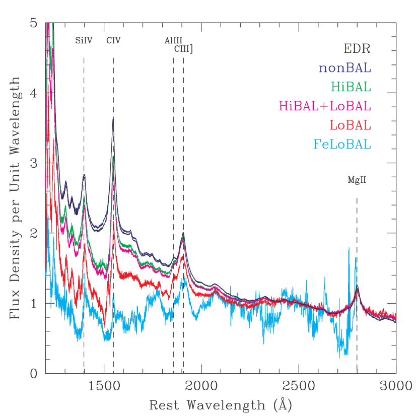
Figure 1: The normalized, geometric composite spectra of — from top to bottom — nonBALs (blue), the full EDR quasar sample (black), HiBALs (excluding LoBALs and FeLoBALs, green), HiBALs and LoBALs (all BALQSOs except for FeLoBALs, magenta), LoBALs (red), and FeLoBALs (cyan). The spectra are normalized at $2500\,{\rm\AA}$. Except for the FeLoBAL composite which exhibits excess emission at long wavelengths, the spectra are similar at wavelengths above 2400 Å, but the BALQSO composite spectra show clear flux deficits at shorter wavelengths as compared to the nonBAL composite spectrum. The FeLoBAL composite includes only a small number of spectra and is for illustrative purposes only.

Reichard et al. (2003) created geometric mean composite spectra of the classes of BALQSOs. The 185 complete-sample BALQSOs and 39 supplementary BALQSOs were partitioned into a HiBAL class (180 objects with high-ionization broad absorption troughs, such as C IV, but without low-ionization broad absorption lines, such as Mg II), a LoBAL class (34 objects with high- and low-ionization broad absorption lines), a combined class of both HiBALs and LoBALs, and the small class of FeLoBALs. Reichard et al. (2003) also created a nonBAL sample and composite spectrum of 892 objects with similar redshift and absolute $i^{*}$ magnitudes to the total BALQSO sample. The composite spectra (including the EDR composite spectrum), normalized to unity at a rest wavelength of 2500 Å, are reproduced in Figure 1; the size and properties (see below) of the samples are given in Table 1. The signal-to-noise ratio is significantly lower in the LoBAL and FeLoBAL composite spectra than in the other composites because of the small sample sizes.

A composite spectrum created from a sample of reddened power-law spectra will possess a mean spectral index and a mean reddening. For geometric mean composites, the composite spectral index and reddening are the arithmetic mean spectral index and arithmetic mean reddening of the individual spectra, as we show in the Appendix. Each of our composite spectra are formed by the geometric mean approach. Thus comparisons of spectral indices and reddening in different composite spectra are equivalent to comparisons of the general subsamples that comprise the composites.

3.2 Continuum Fitting with a Composite Spectrum

In our investigation of the continuum differences between quasar types, we will rely upon the composite-fitting algorithm described by Reichard et al. (2003), since that method allows some freedom in disentangling the power-law continuum from any curvature in the spectrum (from dust extinction, for example). The method is explained in detail by Reichard et al. (2003), but we provide a brief overview here.

Quasar continua are often described by a power law relation $f_{\lambda}\propto\lambda^{\alpha}$ with a spectral index $\alpha\;(=\alpha_{\lambda}=-2-\alpha_{\nu})$ and roughly Gaussian emission-line profiles. In this paper we make the assumption that deviations from a power law times the template composite spectrum over a wide wavelength range can be modeled as extinction by dust. The continuum is represented by

$$f_{\lambda}\propto g_{\lambda}\lambda^{\alpha}10^{-aE(B-V)\xi(\lambda)},$$ (1)

where $\lambda$ is in units of microns, $g_{\lambda}$ is the template composite spectrum, $a=0.4(1+R_{V})$, and $\xi(\lambda)$ is the extinction curve. We have adopted the SMC extinction curve fit given by Pei (1992), for which the ratio of total to selective absorption is $R_{V}=A_{V}/E(B-V)=2.93$. We choose the SMC curve because — unlike those of the LMC and the Milky Way — it lacks the “2200 Å bump”, which has never been conclusively seen from quasar host galaxy dust, possibly due to the destruction of small graphite grains by the quasar’s radiation field (e.g., Perna, Lazzati, & Fiore 2003).

We investigate the continuum properties with three different fitting procedures. If spectral indices alone are the reason that BALQSOs are intrinsically redder than nonBALQSOs, then the BALQSO and nonBALQSO composite spectra might be matched by a simple change of spectral index. On the other hand, if BALQSOs are really dust reddened and/or if they do not have the same underlying spectral index distribution as nonBALQSOs, then the fits will need to properly account for the lost continuum flux at bluer wavelengths due to dust reddening. Thus, one procedure is a two-parameter fit, where we fit spectra by changing both the power-law spectral index and $E(B-V)$ of a template composite spectrum to match each individual spectrum. We will also fit spectra by allowing only one of these parameters to change. To distinguish these different fits, we will abbreviate them as $P$, for change in the power-law spectral index only, $f_{\lambda}\propto\lambda^{\alpha}$; $R$, for change in reddening only, $f_{\lambda}\propto 10^{-aE(B-V)\xi(\lambda)}$; and $RP$, for change in both the power-law spectral index and reddening, $f_{\lambda}\propto\lambda^{\alpha}10^{-aE(B-V)\xi(\lambda)}$.

The template composite spectrum that we use for our fits is the EDR composite spectrum (all 3814 objects). Although we do not know how much reddening is included in the EDR composite, we arbitrarily define the EDR composite reddening to be zero. Thus, the measured reddening values do not indicate absolute reddening but rather reddening relative to the EDR composite spectrum. For reference, we computed the spectral index of the EDR composite spectrum to be $\alpha_{\lambda}=-1.58$ by fitting a power law to points near $\lambda=$ 1355 $\rm{\AA}\;$and 2240 Å.

4 Broad-band UV/Optical Colors of BALQSOs

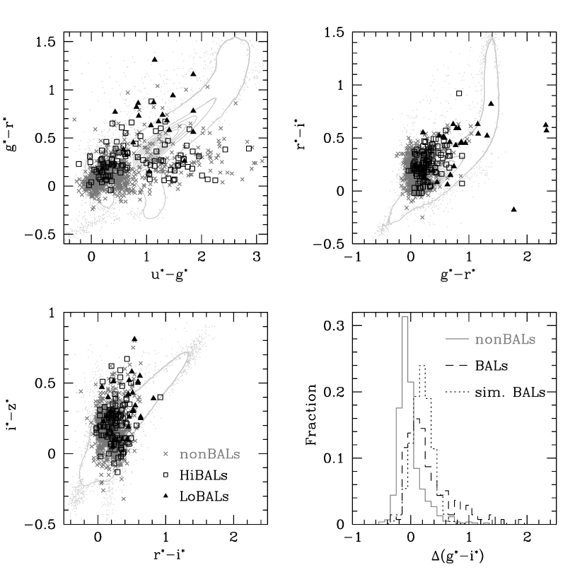
Figure 2: Colors of nonBALs (dark gray “x”s) and BALQSOs (HiBALs, open black squares; LoBALs, filled black triangles) in SDSS color-color-color space for quasars with $1.8\leq z\leq 3.5$. Light gray points and contours show the distribution of all point sources in the SDSS EDR, including quasars, stars and unresolved galaxies; only objects with small errors in each band are included. The lower right hand panel shows the distribution of relative $(g^{*}-i^{*})$ colors, $\Delta(g^{*}-i^{*})$, for both nonBALQSOs and BALQSOs in addition to the distribution for the simulated BALQSOs discussed in Section 8.2.

We can begin addressing the question of the continuum differences between BALQSOs and nonBALQSOs by investigating the differences between their broad-band colors. Menou et al. (2001) and Tolea et al. (2002) have already shown that the broad-band colors of BALQSOs are redder than those of nonBALQSOs. In the color-color plots in Figure 2 we expand upon this result using the full sample of Reichard et al. (2003). The panels in Figure 2 include all EDR nonBALQSOs (gray “x”s) and EDR BALQSOs (open black squares, HiBALs; filled black triangles, LoBALs) with redshifts between 1.8 and 3.5 (where our BALQSO sample is most complete). It is clear that BALQSOs are redder than nonBALQSOs on the average. In particular, it is obvious that the apparently bluest nonBALQSOs (e.g., $g^{*}-r^{*}\lesssim 0$) are greatly underrepresented among the BALQSOs. This result is not simply because of absorption from the BAL troughs themselves. The trough absorption can make the broad-band color of BALQSOs bluer as well as redder, depending on where the redshift of the quasar places the troughs with respect to the filters. Instead, it is the overall flux deficit which spans the entire width of a filter that causes BALQSOs to be redder than nonBALQSOs.

In the bottom right-hand panel, we show that BALQSOs are redder than nonBALQSOs in yet another way. Here we use relative colors (Richards et al. 2001; Richards et al. 2003), which are colors corrected by the median color as a function of redshift and thus are independent of redshift. From these distributions of relative $g^{*}-i^{*}$ color, we find that BALQSOs have an even more pronounced tail of red colors than do nonBALQSOs.

5 BALQSO/nonBALQSO Continuum Comparison

Extending the broad-band results, using spectral analysis, we now investigate the finding of previous authors that LoBALs are redder than both nonBALs and HiBALs (e.g., Weymann et al. 1991) and that even HiBALs are redder than nonBALs (e.g., Brotherton et al. 2001). We examine the continuum (i.e., color) differences between our BALQSO and nonBALQSO samples in two ways: first by comparing the ensemble averages in the form of composite spectra and second in terms of the spectral indices and reddening values that result from our fits of each individual quasar to a template. Emission and absorption properties of BALQSOs will be discussed in § 6.

5.1 Composite Spectra Measurements

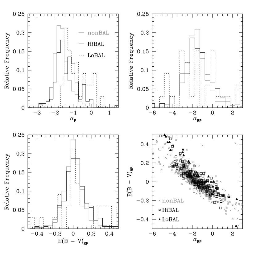
Figure 3: Distribution of spectral indices and reddening values for the $P$-fit and $RP$-fit procedures. Solid black lines indicate HiBALs, dashed black lines indicate LoBALs, while solid gray lines indicate nonBALQSOs. In the bottom right-hand panel, gray “x”’s are for nonBALs, open black squares for HiBALs and filled black triangles for LoBALs.

To compare the composite spectra continua, the EDR composite spectrum is fitted to each of the BALQSO composite spectra by the $\chi^{2}$-minimization procedure described in § 3 of Reichard et al. (2003). In short, the spectra are compared in wavelength regions where emission and absorption are typically absent. The algorithm iteratively searches for values of the spectral index and reddening that provides the best fit. The resulting $\alpha_{P}$, [$\alpha_{RP},E(B-V)_{RP}$], and $E(B-V)_{R}$ values are given in Table 1. The single-parameter fits yield consistent results that suggest increased reddening with increasing BAL strength. The two-parameter fits are more difficult to interpret, especially given the strong degeneracy between spectral index and reddening when performing a two-parameter fit; see Figure 3 in Reichard et al. (2003).

As a simplistic check on our method and code, we fit the EDR quasar composite spectrum to itself and indeed found that the algorithm returns the appropriate values, specifically, $\alpha_{P}=\alpha_{RP}=-1.58$ and relative reddening $E_{R}=E_{RP}=0$. The nonBAL composite is slightly bluer ($\alpha_{P}=-1.61$) than the EDR composite spectrum ($\alpha_{P}=-1.58$) and is best fit by lower reddening values than the EDR composite. This result is to be expected if BALQSOs are redder than nonBALQSOs since the EDR composite spectrum includes BALQSOs.

We find that both the HiBAL and HiBAL+LoBAL composite spectra are redder than the nonBALQSO composite spectrum, having power-law fits with spectral indices $\alpha_{P}=-1.39$ and $-1.29$, respectively. In addition, for the $R$-fit model, both of these composites require reddening relative to the EDR composite spectrum: $E(B-V)=0.023$ and $0.032$, respectively. The redder values for the HiBAL+LoBAL composite spectrum suggest that the LoBAL population is redder than the HiBAL population. Indeed, the LoBAL composite spectrum has the reddest power-law-only fit, $\alpha_{P}=-0.93$, and requires the largest correction for the dust-only fit, $E_{R}(B-V)=0.077$. A large reddening value is also required for the $RP$-fit of the LoBAL composite. However, the interpretation of $RP$-fit values is less clear, and we are reluctant to place any absolute physical importance on these values due to the degeneracy described above (but see the next section, as well as § 7 below). Nevertheless, the single-parameter fits unambiguously demonstrate that the sequence of nonBALs, HiBALs, and LoBALs is a sequence of quasars with increasingly red colors. This result is consistent with the finding of Brotherton et al. (2001) for their radio-selected sample of HiBALs and inconsistent with the original findings of (Weymann et al. 1991); both of these previous results are based on much smaller samples.

5.2 Individual Measurements

We derive qualitatively similar results from the fits to individual quasars, as seen in Figure 3. The upper, left-hand panel shows that, for the $P$-fits, BALQSOs (both HiBALs and LoBALs) have a distribution of spectral indices which is shifted slightly to the red (more positive values of $\alpha_{P}=\alpha_{\lambda}$) and has a much larger fraction of quasars in the red tail. For the $RP$-fits (upper, right-hand and lower, left-hand panels) the derived spectral indices for both BALQSOs and nonBALQSOs are similar, but the best-fit reddening values are skewed slightly to the red.

The $RP$-fit results are better illustrated in the lower, right-hand panel where we plot $\alpha_{RP}$ versus $E(B-V)_{RP}$. The $\alpha_{RP}$ values are clearly non-physical since the range of values is much larger than the observed distribution of spectral indices in quasars and since there is a degeneracy between $E(B-V)$ and $\alpha$. Although there is a true $\chi^{2}$-minimizing pair of spectral index and reddening values for the $RP$-fits, the degeneracy between $E(B-V)$ and $\alpha$ means that the two-parameter $RP$ fitting method cannot be used to determine unique, physical spectral indices and reddening values. As such, the $RP$ spectral indices and reddening values must be considered only mathematical values to reproduce the continua. Nevertheless, we can clearly see that at a given value of $\alpha_{RP}$, BALQSOs (LoBALs in particular) are redder than nonBALQSOs as measured by $E(B-V)_{RP}$; this result cannot be caused by the degeneracy between the two parameters of the $RP$-fit. A two-dimensional K-S test (Fasano & Franceschini 1987) shows that the nonBALQSO and BALQSO distributions in the [$E(B-V)_{RP},\alpha_{RP}$] plane are different at the 99.9999% confidence level ($\simeq 5\sigma$). The HiBAL and LoBAL (including FeLoBAL) distributions are different at the 99.56% confidence level ($\simeq 2.8\sigma$). Finally, as we shall discuss in § 7.2, we have reason to believe that the $RP$-fit values may still be useful in a relative sense.

5.3 The Form of the Reddening

Having shown that both LoBALs and HiBALs are redder than nonBALQSOs and that LoBALs are redder than HiBALs, we explore the question of the origin of the reddening. Specifically, we ask whether BALQSOs simply have redder power-law spectral indices or if they are more dust reddened. A combination of both is also possible, as are non-dust-related reddening scenarios; for example Figures 12–14 in Hubeny et al. (2000) show that redder quasars might simply be observed more face-on, have lower accretion rates, and/or have larger black hole masses, respectively. Since previous work has shown that SMC-like dust reddening might be able to account for the redness of BALQSOs, we adopt that law for our purposes here.

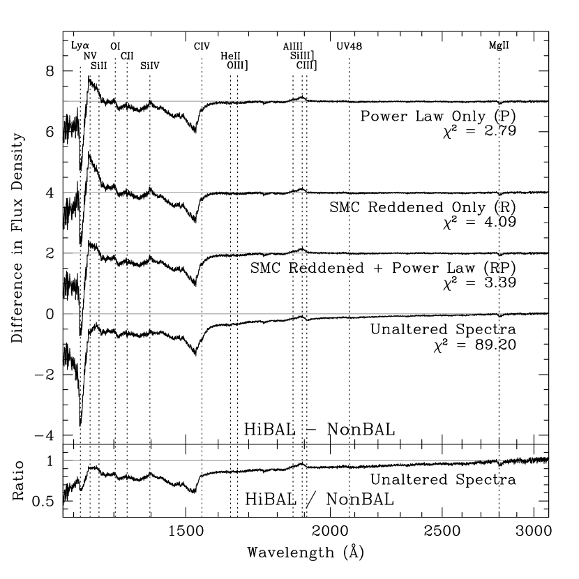
Figure 4: Difference spectra for the HiBAL and nonBAL composite spectra after matching continua via the various fitting procedures. See text (§ 5.3) for details. Compare to Weymann et al. (1991), Figures 4 and 5. The bottom panel shows the ratio of the unaltered spectra rather than the difference. The $\chi^{2}$ values are intended as a goodness-of-fit measure for continuum regions between 1620 and 4100 Å.

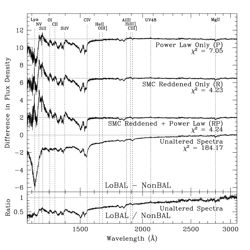
Figure 5: Difference spectra for the LoBAL and nonBAL composite spectra, as in Figure 4. Compare to Weymann et al. (1991), Figure 6.

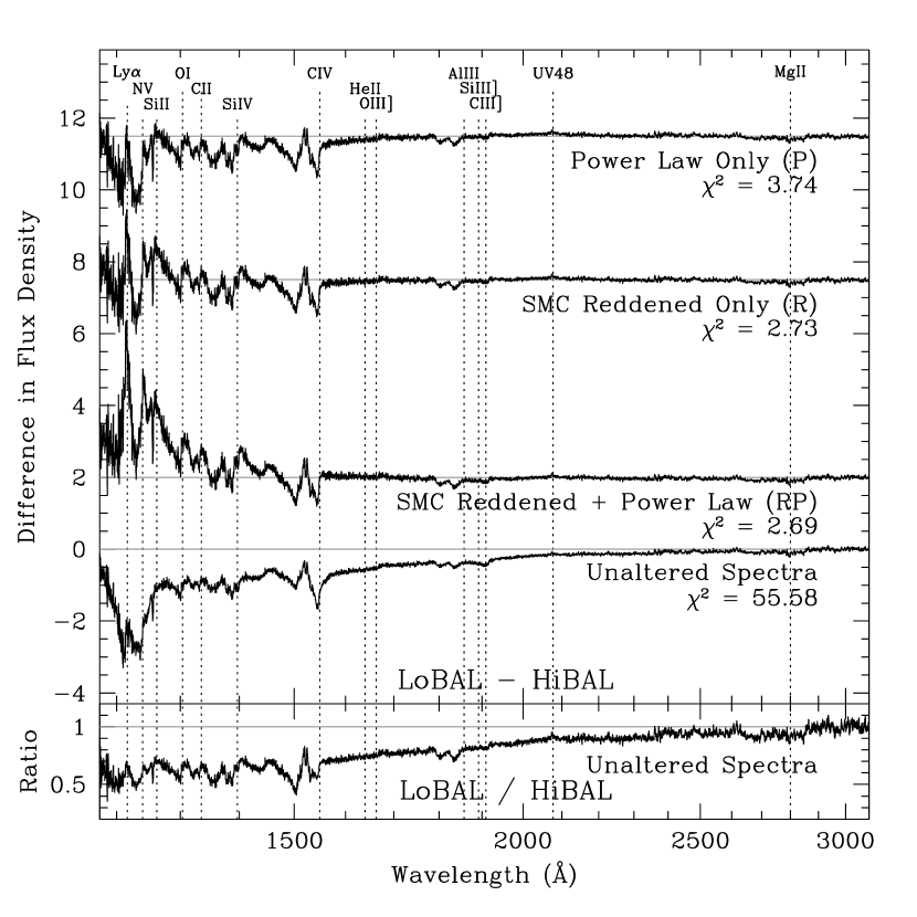
Figure 6: Difference spectra for the LoBAL and HiBAL composite spectra, as in Figure 4.

To aid in our analysis, we present the differences between the nonBAL, HiBAL, and LoBAL composite spectra in Figures 4–6. In each case we present the difference spectra that result from modifying the BALQSO composites by all three of our fitting methods ($P$, $R$, and $RP$) in addition to showing the unaltered difference spectra (i.e., no changes in spectral index or reddening, but are normalized to unity at 2900 Å). Because the EDR and nonBAL composite spectra are similar, as are the HiBAL+LoBAL and HiBAL composite spectra, we have chosen to use only the composite spectra of the mutually exclusive nonBAL, HiBAL, and LoBAL classes in the rest of our analysis.

The $P$-fit (top spectrum in Figs. 4–6) was achieved by changing only the spectral index $\alpha_{P}$ of each of the HiBAL and LoBAL composites. From the $P$-fits, one could make an argument for BALQSOs simply having redder spectral indices than nonBALQSOs. Similarly, applying only the SMC ($R$-fit) reddening law to the composites (second spectrum in Figs. 4–6) suggests that dust-only reddening might just as adequately account for the color differences between BALQSOs and nonBALQSOs. Finally, the $RP$-fit difference spectra are plotted as the third spectrum in each of Figures 4–6, using spectral indices and relative reddening from Table 1. As with both of the previous fitting procedures, the $RP$-fit does a reasonably good job of correcting for the color differences between the BALQSOs and the nonBALs.

For wavelengths longer than about $1700\,{\rm\AA}$, each of the three reddening corrections to the BALQSOs reproduces the continuum of the nonBALs reasonably well. Thus, it is difficult to use this analysis alone to answer the question posed above regarding the nature of the reddening in BALQSOs. Expanding our wavelength baseline via UV and near-IR spectra of our objects would clearly be valuable in terms of answering the question of the form of the reddening. Nevertheless, we have shown that the reddening that is observed in our BALQSO sample is certainly consistent with SMC-like dust as suggested by previous authors. Furthermore, at least some contribution from reddening is favored for LoBALs, as seen by the $\chi^{2}$ of the fits in Figures 5 and 6 and our analysis in § 7.2.

If BALQSOs and nonBALQSOs have the same intrinsic spectral index distribution and BALQSOs are reddened by SMC-like dust, then the average reddening for HiBALs is $E(B-V)=0.023$ and for LoBALs is $E(B-V)=0.077$ (as compared to the EDR composite spectrum, which is reddened by $E(B-V)\sim 0.004$ as compared to the nonBALQSO composite). These numbers can be compared to Sprayberry & Foltz (1992) and Brotherton et al. (2001) who each applied an SMC reddening law and found that $E_{Lo}-E_{Hi}\sim 0.1$ was needed to account for flux deficits in LoBALs as compared to HiBALs. Our results suggest a smaller differential reddening between the HiBALs and LoBALs. This small difference between our results and previous results may be related to the fact that the SDSS EDR BALQSO catalog includes a much larger fraction of BALQSOs with smaller balnicity indices than the Weymann et al. (1991) sample. One way that our smaller differential reddening result might be understood is if BALQSOs with larger balnicity indices are more heavily reddened; a larger sample is needed to determine if this is actually the case.

6 Emission and Absorption Properties

In addition to investigating the differences in the continua and colors of BALQSOs, it is also important to examine the differences and similarities in their emission lines. In particular, if BALQSOs and nonBALQSOs are drawn from the same parent population, they are likely to have similar emission-line properties (Weymann et al. 1991). Thus, we now revisit Figures 4–6 with emission lines instead of continua in mind. At the same time we will also comment on significant differences in the absorption line properties of the different BALQSO samples.

We begin the emission-line analysis by examining the emission-line region near Mg II. In each panel of Figure 4 the Mg II emission lines are similar for HiBALs and nonBALs, except that there appears to be a slight dearth of emission in HiBALs just redward of the expected line peak (as evidenced by negative flux in the HiBAL minus nonBAL difference spectrum). This result holds true as well for the LoBAL composite in Figure 5, where we see evidence for a broader decrement of flux in the red wing of Mg II. We also note that strong, prominent absorption troughs, such as those found blueward of C IV and Al III, are absent blueward of Mg II in the LoBAL composite. This absence is not unexpected since the creation of composite spectra tends to wipe out features that are not persistent from spectrum to spectrum. Since the Mg II absorption troughs can occur at different velocities from the emission line peak, the apparent strength of the absorption is diminished in the composite spectrum.

Moving to shorter wavelengths, we find that the HiBAL composite shows no excess in the UV48 complex of Fe III at $2080\,{\rm\AA}$, but that there may be a slight excess in LoBALs. Weymann et al. (1991) reported an excess at this wavelength among their LoBALs and also found that the strength of this feature correlates with the balnicity index for HiBALs as well as LoBALs.

Continuing on to the complex of emission near C III] $\lambda 1909$, we find a small excess of emission in the Al III and Si III] region of the HiBAL composite, which Weymann et al. (1991) suggested is likely due to Fe III or Fe II emission. However, we do not see any excess longward of the peak of C III] which would be expected from Fe III UV34. In the LoBAL composite, this same excess may still persist, but more significant is a decrement of flux at the centroid of C III].

No strong absorption from Al III is seen in the HiBAL composite, but the LoBAL composite exhibits two prominent absorption troughs near $1804\,{\rm\AA}$ and $1835\,{\rm\AA}$, with a peak near $1819\,{\rm\AA}$. A third depression is found near $1750\,{\rm\AA}$ and may have a weaker counterpart in the HiBAL composite. The Al III absorption lines are quite strong in the LoBAL composite, whereas the Mg II troughs which were used to define the LoBALs are relatively absent, suggesting perhaps that Al III is a better indicator of LoBALs or that Al III absorption has a more consistent velocity distribution from quasar to quasar.

In the composite spectra shown in Figure 1, He II $\lambda 1640$ emission appears to be slightly weaker in BALQSOs than in nonBALQSOs. The difference spectra in Figures 4 and 5 also exhibit this weakness.

At the location of C IV we see some interesting differences in the spectra. First, we confirm the reality of the “droop” in the difference spectrum that was reported by Weymann et al. (1991). This “droop” occurs between the C IV emission peak and $\sim 1600\,{\rm\AA}$ and is seen in both the HiBAL composite and LoBAL composite, as shown in Figures 4 and 5. We note that the form of this “droop” is similar to the C IV emission line flux decrement that was observed in quasars with large C IV emission-line blueshifts (Richards et al. 2002b) and may be an indication that BALQSOs have larger-than-average C IV emission-line blueshifts; see § 7.

In addition to this “droop” is the obvious decrement of flux blueward of the emission-line peak that is caused by the C IV BAL troughs themselves. The absorption becomes significantly more pronounced in the HiBAL composite near the expected peak of C IV (i.e., at zero velocity with respect to the quasar redshift); in the LoBAL composite, the change at zero velocity is even more dramatic. C IV broad absorption troughs thus penetrate to velocities less than the minimum velocity of the C IV balnicity index ($3000\,{\rm km\,s^{-1}}$ at 1534.5 Å). The C IV trough in the HiBAL composite has a minimum near $1520\,{\rm\AA}$ with a weaker shoulder that extends from about $1500\,{\rm\AA}$ to perhaps as blue as the peak of Si IV+O IV]. The LoBAL composite difference spectrum exhibits two distinct C IV troughs near $1502\,{\rm\AA}$ and $1541\,{\rm\AA}$ that are separated by a peak near $1518\,{\rm\AA}$ (which is roughly consistent with the 1520 $\rm{\AA}\;$minimum of the C IV trough in the HiBAL composite difference spectrum). The structure in the composite spectra troughs is particularly interesting since, as described above, the construction of composites tends to average out any structure that is not persistent from quasar to quasar.

There is absorption just blueward of the Si IV+O IV] emission-line peak in both the HiBAL and LoBAL composite spectra. In the LoBAL composite difference spectrum, the absorption is double-troughed (with minima near $1356\,{\rm\AA}$ and $1386\,{\rm\AA}$ and separated by a peak near $1370\,{\rm\AA}$). We see no obvious trend in the separation of the double troughs in Al III, C IV and Si IV that are seen in the LoBAL composite difference spectrum, but for all three of these systems the peak between the troughs is roughly $6000\,{\rm km\,s^{-1}}$ from the expected emission-line center, which is suggestive of the radiative acceleration “ghost of Ly$\alpha$” effect described by Arav (1996).

Toward the bluer end of the spectra, the continuum fits are not nearly as good and it becomes difficult to tell whether the features that we see are the result of excess emission or absorption. Nevertheless, there are a few notable features. The LoBAL composite difference spectrum displays absorption just blueward of each of the C II $\lambda 1335$, O I/Si II $\lambda 1304$ and Si II $\lambda 1262$ emission lines. Finally, in the HiBAL composite difference spectrum there is an excess of flux between N V and Si II that may be similar to the excess N V emission that Weymann et al. (1991) reported for their BALQSOs.

7 The BALQSO Parent Sample

7.1 Comparison with Color and Emission-Line Shift Composites

One of the primary reasons for comparing the continua and emission lines of BALQSOs to nonBALQSOs is to determine if they are drawn from the same parent population. Although our BALQSOs and nonBALQSOs are selected in the same manner using only the optical/UV part of the spectrum, the SDSS selection algorithm is sensitive to a wide range of optical/UV properties. As such, we might expect to see differences in the UV/optical properties of BALQSOs if they are indeed drawn from a different parent sample. Such differences should be more noticeable at other wavelengths, particularly the IR and sub-mm (where dust is seen in emission rather than absorption); however, recent sub-mm observations show no significant differences between BALQSOs and nonBALQSOs (Lewis et al. 2003; Willott et al. 2003).

We consider the issue of the BALQSO parent sample by examining the continuum and emission-line properties of BALQSOs as compared to normal quasars. In previous investigations of SDSS quasars, we found significant and possibly related trends in the spectra as a function of both the C IV emission-line blueshift (Richards et al. 2002b) and the broad-band colors (Richards et al. 2003). In Figure 7, we plot the relative $g-i$ color, $\Delta(g-i)$, against C IV blueshift for bright ($i<18.1$) EDR quasars. We find a weak anti-correlation: quasars with little or no blueshift are rarely as blue as $\Delta(g-i)\sim-0.1$, while relative colors near $-0.1$ are typical for objects with high blueshifts. Quasars with larger C IV blueshifts thus appear to have bluer optical colors.

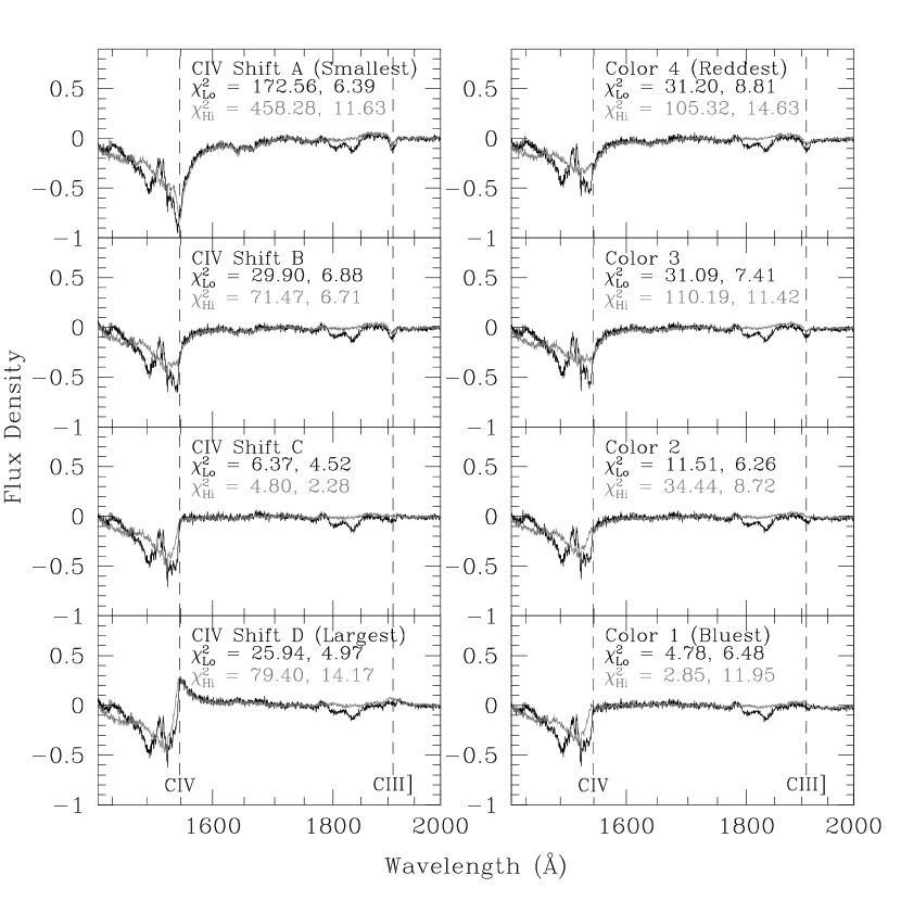
Figure 8: HiBAL (gray) and LoBAL (black) composite spectra compared with composite spectra of quasars with respect to extremes in emission-line blueshifts and broad-band colors. The left panels show difference spectra with respect to C IV blueshift, whereas the right panels show difference spectra with respect to color. The two $\chi^{2}$ values given in each panel are for the red wing of C IV and the entire C III] emission-line region, respectively. Comparison of these two regions suggests that BALQSOs tend to be intrinsically bluer than average and have larger than average C IV emission-line blueshifts.

Since previous work has shown that the emission features change as a function of C IV blueshift and color, we suggest that it is possible to learn something about the intrinsic properties of BALQSOs by comparing their emission lines to the emission lines in the C IV blueshift and color composites. In Figure 8, we compare our HiBAL and LoBAL composite spectra in the spectral region covering the C IV and C III] emission lines to the C IV shift composites (left panels) from Richards et al. (2002b) and to the color composite spectra (right panels) from Richards et al. (2003). We specifically examine the composites in the red wing of the C IV emission line and in the vicinity of the He II $1640\,{\rm\AA}$ and C III] emission lines. Since we wish to concentrate on the similarities and differences of the emission lines in these composites, we have first removed the overall continua from each of the composites using the $RP$-fit method described above.

In the left panels of Figure 8, we see that the small C IV shift composite is a rather poor fit to either the HiBAL or LoBAL composite spectra since the difference spectra deviate from zero in the red wing of C IV emission, near He II and at the peak of C III]). On the other hand, the large C IV shift composite appears to over correct for the “droop” redward of C IV emission. Both HiBALs and LoBALs appear to be best fit (in the red wing of C IV and near both He II and C III]) by the composite with the second largest C IV emission-line blueshift, which suggests that BALQSOs may be preferentially found among quasars with large C IV shifts. Since BALQSOs are intermediate between the extremes of measured C IV blueshifts, a distinct BALQSO parent population is not needed.

Similarly, when we compare our BALQSO composites to the composite spectra as a function of color, we find that the BALQSOs are not equally well described by each of the color composites. The reddest composite disagrees more in the red wing of C IV and at the peak of C III] than the bluest composite, which provides the best fit. Thus BALQSOs may be drawn from a part of the parent sample which is intrinsically bluer than average. As with the blueshifts, although there are differences in color between BALQSOs and nonBALQSOs, they are not larger than the known differences among nonBALQSOs themselves, which suggests that there is no need for a separate parent population.

7.2 BALQSO Composites as a Function of Fitted Spectral Indices

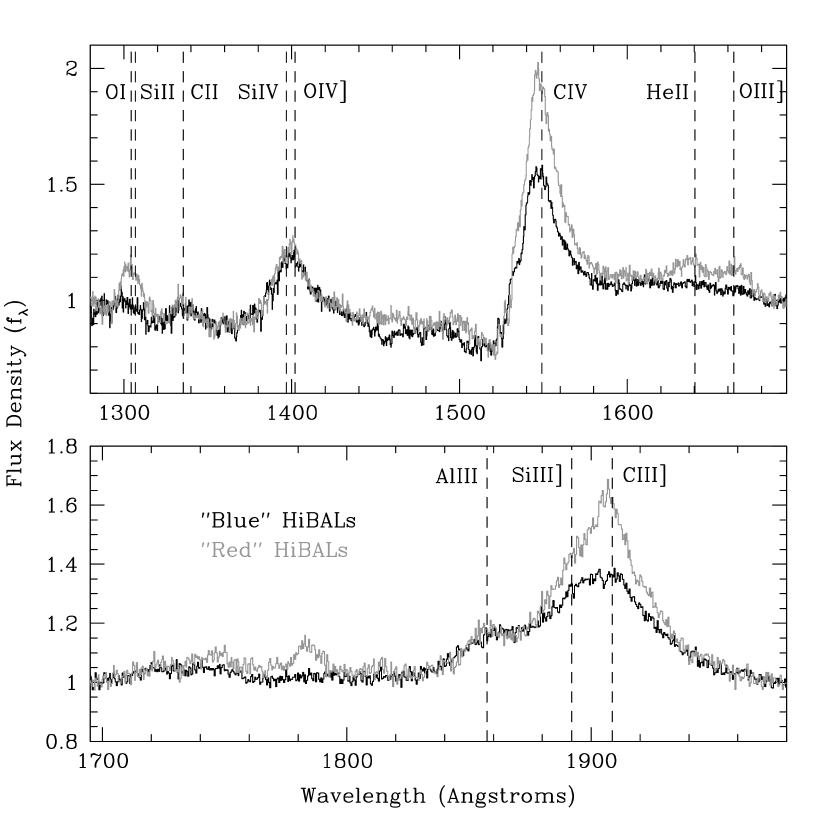
Figure 9: Composite spectra of HiBALs whose $RP$-fits yield intrinsically blue spectral indices (black line) and intrinsically red spectral indices (gray line). Each composite is the average of $\sim 41$ quasars.

The above results suggest that BALQSOs tend to have blue intrinsic optical colors and moderately large C IV blueshift; however, the situation is more complicated than that. Another way to address the issue of the intrinsic color of BALQSOs is to use the results from our $RP$-fits to the individual quasar spectra. That is, we can ask whether the relative spectral indices that result from these $RP$-fits are meaningful even though we know that the absolute values are not necessarily physical. If we assume that the relative $\alpha_{RP}$ values are both meaningful and representative of intrinsic color, we can create and compare composite HiBAL spectra as a function of ”intrinsic” color. We have divided the “complete” sample of 124 HiBAL quasars from the EDR BALQSO catalog into three equal parts according to their $\alpha_{RP}$ values. The bluest and reddest composites that result from these subsamples are shown in Figure 9; the middle composite (not shown) has intermediate properties.

We see that the red HiBALs have emission lines with much larger equivalent widths — consistent with the results of Richards et al. (2003), where bluer quasars were found to have weaker emission lines than redder quasars. There also appears to be a difference in the absorption line troughs between the blue and red HiBAL samples. The blue HiBALs appear to have strong absorption at higher velocities ($\lambda<1510\,{\rm\AA}$) and the red HiBALs have relatively stronger absorption closer to the emission-line peak ($\lambda\sim 1520\,{\rm\AA}$) — similar to “miniBALs” or the so-called “associated” absorption systems (Foltz et al. 1986) found in radio-loud quasars. Although these absorption features are relatively weak, we reemphasize that even the weak composite features must be persistent in the majority of the input spectra, otherwise the features would be washed out in the composites.

7.3 Conclusions with Regard to the BALQSO Parent Population

We suggest that the likelihood of a quasar having BAL-like intrinsic absorption (and the type of absorption) is a function of some intrinsic properties of the quasars (i.e., some intrinsic property or properties determine how likely a quasar is to have BAL troughs and how large a solid angle the flow covers). In the optical/UV, BALQSOs tend towards the region of multidimensional parameter space characterized by bluer colors and larger C IV blueshift (which presumably is tied to more physical properties such as luminosity and/or accretion rate). Although the BALQSOs do appear to favor certain regions of parameter space, their properties span a good portion of that space and do not appear to be disjoint from the distribution of nonBALQSOs. Thus we conclude that the parent samples of BALQSOs and nonBALQSOs are the same — at least for our optically selected sample.

The differences between BALQSOs and nonBALQSOs (and among BALQSOs themselves) could then be due to luminosity (Corbin 1990), accretion rate (Boroson 2002), inclination (Weymann et al. 1991), some other intrinsic property, or a combination thereof. It is difficult to know which of these is primary. The velocity asymmetry in the C IV emission line is suggestive of an obscuration-induced orientation effect (whether external, i.e. line of sight orientation, or internal, i.e. the opening angle of the disk wind), which might be driven by another parameter such as luminosity or accretion rate (e.g., Elvis 2000).

8 The BALQSO Fraction

The differences in the spectra of BALQSOs compared to nonBALs must be taken into account when determining the fraction of quasars that are BALQSOs. In the following sections, we first present the raw BALQSO fraction as a function of redshift. We then use the color properties of BALQSOs to account for color-induced redshift selection effects which result in a corrected BAL fraction as a function of redshift.

8.1 Raw Fractions

Several estimates have been made of the fraction of quasars that show broad absorption troughs. Weymann et al. (1991) estimated a BALQSO fraction of 12% (for $1.5\lesssim z\lesssim 3.0$), while Hewett & Foltz (2003) found an observed fraction of $15\pm 3\%$ (and an intrinsic fraction of $22\pm 4\%$) in the same redshift range. Our uncorrected BALQSO fraction falls between those two results: we measure $14.0\pm 1.0$% (185 BALQSOs out of 1318 quasars with $1.7\leq z\leq 4.2$), similar to the 15% found by Tolea et al. (2002) using mostly the same data set. Sprayberry & Foltz (1992) estimated that the LoBAL fraction of BALQSOs is near 17% (1.5% of all quasars). Since we can identify LoBALs when Mg II or Al III broad absorption is present, we can give a LoBAL fraction for the redshift range $1.7\leq z\leq 3.9$. In this range, our results yield an uncorrected LoBAL fraction of $13\pm 3$% (24/181) among BALQSOs or about $1.9^{+0.5}_{-0.4}$% (24/1291) of the quasar sample. We have not investigated the fraction of BALQSOs as a function of radio power; see Becker et al. (2001) for such a study using the FBQS sample.

8.2 Selection Effects

To determine the true BALQSO fraction, we must investigate the completeness of the SDSS BALQSO sample and apply corrections to our observed fraction. For the Weymann et al. (1991) sample, it was necessary to correct the BALQSO fraction for absorption by the BAL trough itself in the $B$-band that was used to select quasars in the LBQS. The SDSS sample largely avoids that problem since SDSS quasars are selected using an $i$-band magnitude limit. For SDSS quasars with $z\lesssim 3.5$ no correction is needed for BAL absorption in the $i$ band. Above that redshift a correction is needed, but instead we will simply choose to limit our analysis to redshifts where no correction for $i$-band absorption is needed.

Despite this selection rule, there are several other important corrections that are needed in order to determine the “true” fraction of BALQSOs in our sample.

First, in terms of the initial selection of quasars, we have ignored the fact that the limiting magnitude changes by a full magnitude between the low-$z$ and high-$z$ ($z\gtrsim 3$) selection criteria. Also, roughly 20% of the EDR quasars in the redshift range that can be searched for C IV broad absorption were selected for spectroscopy on the basis of “serendipity” (Stoughton et al. 2002). Such quasars pose a particular problem since serendipity selection uses a fainter magnitude limit than was used for quasar selection and is based largely on availability of fibers for a given plate, and therefore has an extremely complicated selection function. The raw statistics presented here assume that the statistics of BALQSO incidence in this set are the same as in the sample collected on the basis of well-defined color criteria. In the next section, we will correct for both the redshift dependent magnitude differences and the serendipity selection effect by imposing a more restrictive selection criteria.

Second, reddening due to dust extinction may extinct quasars enough to fall out of our magnitude-limited sample. This effect could be significant, but we make only a simple estimate of it for now (see § 8.3) and defer a full analysis to a future paper. Fortunately, the SDSS quasar selection algorithm must be more complete to dust extincted quasars than previous optically-selected BALQSO samples in part because of the use of the $i$-band instead of the $B$-band as the limiting magnitude filter. It is also important to realize that this effect is a function of redshift and that higher redshift BALQSOs are more likely to fall out of the sample than lower redshift BALQSOs since high redshift quasars sample shorter, rest-frame wavelengths, that is, the most strongly affected by an SMC-like reddening curve.

Third, since BALQSOs appear to be redder than average, their selection function will not depend on redshift in the same way as for the nonBAL sample of SDSS quasars. We show below that quasars with $2.3\lesssim z\lesssim 2.6$ that are very red are more likely to find themselves embedded in the stellar locus than normal quasars and thus are less likely to be selected as quasar candidates. On the other hand, quasars with $2.6\lesssim z\lesssim 2.9$ are actually more likely to be selected if they are very red (as long as they are not heavily extincted, of course) since their colors will tend to push them out of the stellar locus. Hewett & Foltz (2003) have independently commented on the importance of this effect.

In a preliminary attempt to determine corrections for color-dependent selection effects as a function of redshift in the range $1.7\leq z\leq 3.45$, we determined theoretical colors as a function of redshift by passing both the EDR and HiBAL composite quasar spectra through the SDSS filter curves. Color differences between the average quasar and the average HiBAL quasar were then determined as a function of redshift in the redshift ranges where both composite spectra span the SDSS filters. We then applied these color corrections to the simulated quasar colors (Fan 1999; Richards et al. 2001) that were used to test the SDSS quasar target selection algorithm (Richards et al. 2002a). We compare the color distribution of the simulated BALQSOs to real BALQSOs in the bottom right-hand panel of Figure 2. These simulated BALQSO colors were processed through the SDSS quasar target selection algorithm (Richards et al. 2002a). The results are shown in the top panel of Figure 10, where we show the number of normal quasars selected (as a function of redshift) by the solid line and the number of “BAL” quasars selected by the dashed line. Only about half of the model “BAL” quasars were selected between redshifts 2.4 and 2.6, while similarly inefficient selection of normal quasars occurs at slightly higher redshifts, resulting in a redshift correction as shown in the lower panel of Figure 10. The estimated correction factor rises to 2 near $z\sim 2.4$ and drops to near 0.25 at $z\sim 2.75$. Thus the raw BALQSO fraction may be well estimated at $z<2.2$, underestimated by a factor of 2 at $z\sim 2.4$, and overestimated by a factor of 4 at $z\sim 2.75$.

These correction factors themselves are subject to some uncertainty. By applying the average HiBAL reddening (curvature) correction to each of the simulated quasars, we will obviously be over estimating the correction for some objects and underestimating it for others; thus we may be over- or underestimating the strength of the correction function. In addition, any misestimates of the correction function may themselves be a function of redshift. Lastly, we have made the assumption that the amount of reddening is independent of the quasar’s intrinsic color. If, for example, intrinsically blue or intrinsically red quasars are more (or less) likely to be redder than average when they are BALQSOs, then our correction fractions will be skewed. However, if BALQSOs are really apparently redder than the average quasar, as seems to be the case, then applying this averaged correction is better than not applying any correction at all.

8.3 Corrected Fractions

Using these corrections, we calculate the true BALQSO fraction as a function of redshift by applying these corrections to the raw BALQSO fraction as a function of redshift. In the top panel of Figure 11 we show the raw fractions for both our data set (solid line) and the Tolea et al. (2002) data set (dotted line). In the bottom panel of the same figure, we show the BALQSO fraction as defined by our fitted composite spectrum (FCS) method after applying the above correction for reddening (dashed line). The raw fraction histogram shows a clear excess of BALQSOs for $2.7\lesssim z\lesssim 2.9$, but this excess may simply be a result of the relative selection probabilities for BALQSOs and nonBALQSOs — the corrected fraction is nearer to 10%. The corrected fraction at $z\sim 2.4$ approaches 50%, but this is a single-bin spike and is likely to be an artifact of the limited resolution of the correction function. Note that while we have a complete sample of BALQSOs from the EDR for $1.7\leq z\leq 4.2$, we are only attempting to correct the BALQSO fractions in the range $1.7\leq z\leq 3.45$.

The BALQSO fraction as a function of redshift is also a function of the algorithm that was used to select the quasars in the first place. Since the EDR quasars were selected using three slightly different algorithms (Stoughton et al. 2002) and since these algorithms differ slightly from the SDSS’s final quasar target selection algorithm (Richards et al. 2002a), we also correct our BALQSO fraction based on those objects that are recovered by this final algorithm (excluding the serendipitous targets discussed above). There are 131 BALQSOs in the resulting sample which is both relatively complete and relatively homogeneous, see Reichard et al. (2003). We have computed corrected BALQSO fractions for the this sample of quasars; this BALQSO fraction is plotted in the bottom panel of Figure 11 as a thick solid line. Except for the spikes that are probably caused by small numbers of objects per bin and the finite resolution of the correction function, the BALQSO fraction is now seen to be roughly constant as a function of redshift between $1.7\leq z\leq 3.45$ and is approximately $13.4\pm 1.2\%$, close to our uncorrected EDR fraction ($14.0\pm 1.0\%$) but with a considerably different redshift distribution. Further work is needed to determine if other selection effects (or more careful consideration of the selection effects discussed herein) would affect the redshift dependence of the BALQSO fraction. We also note that making a correction based on the post-EDR selection algorithm does not guarantee that the resulting EDR BALQSO sample is completely homogeneous, since some quasar candidates in the EDR area selected by the new algorithm will not (yet) have SDSS spectra.

So far, although we have corrected for dust reddening (BALQSOs being redder than average), we have not corrected for dust extinction (BALQSOs falling out of the magnitude limited sample), as considered for the LBQS by Hewett & Foltz (2003). A full treatment of this effect is left for a future paper on a larger SDSS BALQSO sample. We can, however, estimate this correction by considering the reddest quasars. Because BALQSOs are typically more dust reddened, more BALQSOs than normal quasars will have been extincted past the SDSS magnitude limit and removed from our sample. In Richards et al. (2003) we estimated that those quasars with $g-i$ colors 0.3 magnitudes redder than the median quasar color at the same redshift comprise at least 15% of the true quasar population, but only 6% of the observed quasar population. Taking this and the BALQSO fractions among normal and dust reddened quasars into account, we estimate that the extinction-corrected BALQSO fraction is 15.9$\pm$1.4%. This extinction correction is an underestimate in the sense that it considers only the reddest BALQSOs. A more refined estimate seems unlikely to equal the 22$\pm$4% found by Hewett & Foltz (2003) for the LBQS; however, given the uncertainties, the BALQSO fractions for the SDSS and LBQS are both consistent with one of every six quasars being a BALQSO.

Finally, in terms of understanding the origin and physics of BALQSOs, it should be noted that in their attempt to discern between clear outflows and the associated absorber population, it is not surprising to find that the Weymann et al. (1991) BALQSO definition clearly underestimates the fraction of quasars with BAL-like outflows. Thus, even the corrected numbers above represent a lower limit to the fraction of quasars that exhibit strong, intrinsic absorption outflows. The use of a revised balnicity index (e.g., Hall et al. 2002) in the future should help to alleviate this problem.

9 Conclusions

We find that there are substantial differences in the continuum and emission-line properties of HiBAL and LoBAL quasars as compared to nonBALs. On average, HiBALs possesses an amount of reddening $\Delta E(B-V)\approx 0.023$ relative to the average quasar, and LoBALs possess $\Delta E(B-V)\approx 0.077$. Wider wavelength coverage is needed to determine the exact form of this reddening, but SMC-like dust extinction provides an acceptable fit. Our understanding of the origin of these differences may be hampered to some extent by the possibility that our BALQSO and nonBALQSO samples do not have the same intrinsic properties. In particular, we suggest that BALQSOs may be intrinsically bluer (and have weaker, more strongly blue-shifted C IV emission) than nonBALQSOs on the average. The absorption properties may also be a function of intrinsic quasar properties with LoBALs having the most extreme properties. Despite their differences, we suggest that optically-selected BALQSOs are not drawn from a different parent sample than nonBALQSOs, but rather have a bias towards certain intrinsic quasar properties within the same parent sample.

Using our entire sample, we find that the raw, uncorrected fraction of HiBALs is $14\%$, and that Mg II LoBALs comprise at least 1.9% of all quasars. These BAL fractions are not corrected for a variety of selection effects, most notably differential color-induced redshift-dependent selection effects. Using our most complete and homogeneously selected subsample, we extend the results of Tolea et al. (2002) by attempting a correction for color-dependent selection effects as a function of redshift. We find that the corrected HiBAL fraction is $13.4\pm 1.2$% (15.9$\pm$1.4% if we include a dust extinction correction) and is roughly constant with redshift for $1.7\leq z\leq 3.45$. Given the constraints used to classify BALQSOs, this fraction should be taken as a lower limit to the fraction of quasars that have intrinsic outflows along our line of sight.

$$f^{\prime}_{i}(\lambda) \equiv \frac{f_{i}(\lambda)}{f_{i}(\lambda_{0})}=\left(\frac{\lambda}{\lambda_{0}}\right)^{\alpha_{i}}10^{-0.4E_{i}[R(\lambda)-R(\lambda_{0})]},$$ (1)

and thus,

$$f^{\prime}_{i}(\lambda) \propto \lambda^{\alpha_{i}}10^{-0.4E_{i}[R(\lambda)-R(\lambda_{0})]}.$$ (2)

The geometric mean composite $f_{gm}$ is

$$f_{gm}(\lambda) \equiv \left(\prod_{i}f^{\prime}_{i}(\lambda)\right)^{1/n}$$ (3)

$$\propto \lambda^{(\sum_{i}\alpha_{i})/n}10^{-0.4(\sum_{i}E_{i}/n)(R(\lambda)-R(\lambda_{0}))}$$ (4)

$$\propto \lambda^{\langle\alpha_{i}\rangle}10^{-0.4\langle E_{i}\rangle(R(\lambda)-R(\lambda_{0}))},$$ (5)

which is of the same form as Eq. 2. The arithmetic mean spectral index $\langle\alpha_{i}\rangle$ and reddening $\langle E_{i}\rangle$ appear as the spectral index and reddening of the geometric composite spectrum — assuming that the form of the reddening law is the same for all spectra. When the reddening law is not the same for all spectra, the geometric mean composite spectrum no longer yields the arithmetic mean $E(B-V)$, but it still yields the arithmetic mean absorption $\langle A(\lambda)\rangle=\langle E(B-V)\times R(\lambda)\rangle$ at each wavelength. That is, the extinction factor in Equation 5 cannot be simplified beyond $10^{-0.4<A_{i}(\lambda)>}$ because there is no longer a single extinction law which can be factored out from the reddenings $E_{i}$, but since $A_{\lambda}=E(B-V)\times R_{\lambda}$, for each spectrum we have

$$f^{\prime}_{i}(\lambda)\propto\lambda^{\alpha_{i}}10^{-0.4A_{i}}$$

which yields a geometric mean of

$$f_{gm}(\lambda)\propto\lambda^{<\alpha_{i}>}10^{-0.4<A_{i}>}.$$

Figure 7: C IV velocity shift versus relative $g-i$ color, $\Delta(g-i)$, for bright ($i<18.1$) EDR quasars. Quasars with larger C IV emission-line blueshifts appear to have bluer intrinsic colors. The dashed line is a least-squares fit to the data.

Figure 10: Top panel. Number of simulated quasars selected (out of a maximum of 700 in each redshift bin) by the SDSS quasar target selection algorithm for normal quasars (solid line) and simulated “BAL” quasars (dashed line); see text. Bottom panel. The correction factor for raw BALQSO fractions due to redshift-dependent selection effects.

Figure 11: (top) The raw fraction of BALQSOs using the FCS method of Reichard et al. (2003) (solid line) and the method of Tolea et al. (2002) (dashed line). Note that the discrepancy in the first bin simply results from the higher minimum redshift imposed by Tolea et al. (2002) in their sample. (bottom) The fraction of FCS-defined BALQSOs corrected for reddening induced selection effects (dashed line); see text. The solid line shows the distribution of BALQSOs that were also corrected for this selection effect, but that are restricted to those EDR quasars that were also identified as quasar candidates by the SDSS’s final quasar target selection algorithm as described by Richards et al. (2002a). The fully corrected distribution yields a BALQSO fraction of $13.4\pm 1.2$% that is largely independent of redshift. Error bars give 68% confidence intervals (statistical error only).

Table 1: Composite Spectrum Data

	Number of
Class	Objects	$\alpha_{P}$	$(\alpha_{RP}$	$E_{RP})$	$E_{R}$
EDR	3814	$-1.58$	$-1.58$	$0.000$	$0.000$
NonBAL	892	$-1.61$	$-1.60$	$-0.002$	$-0.004$
HiBAL	180	$-1.39$	$-1.23$	$-0.020$	$0.023$
HiBAL+LoBAL	214	$-1.29$	$-1.19$	$-0.012$	$0.032$
LoBAL	34	$-0.93$	$-2.01$	$0.126$	$0.077$
FeLoBAL	10	$\cdots$	$\cdots$	$\cdots$	$\cdots$

Note. — All spectral indices are in terms of $\alpha_{\lambda}$ with $f_{\lambda}\propto\lambda^{\alpha_{\lambda}}$. $E$ represents the reddening relative to the inherent reddening of the EDR composite spectrum, i.e., $E\equiv E(B-V)-<E(B-V)_{EDR}>$. The spectral indices and reddening values are given for the three fits: $P$ for a power law (no reddening), $RP$ for a combination power law and SMC reddening law, and $R$ for an SMC reddening law (no change in spectral index). See § 5.1 for discussion.

References

- Arav (1996) Arav, N. 1996, ApJ, 465, 617
- Becker, Gregg, Hook, McMahon, White, & Helfand (1997) Becker, R. H., Gregg, M. D., Hook, I. M., McMahon, R. G., White, R. L., & Helfand, D. J. 1997, ApJ, 479, 93
- Becker, White, Gregg, Brotherton, Laurent-Muehleisen, & Arav (2000) Becker, R. H., White, R. L., Gregg, M. D., Brotherton, M. S., Laurent-Muehleisen, S. A., & Arav, N. 2000, ApJ, 538, 72
- Becker, White, Gregg, Laurent-Muehleisen, Brotherton, Impey, Chaffee, Richards, Helfand, Lacy, Courbin, & Proctor (2001) Becker, R. H., White, R. L., Gregg, M. D., Laurent-Muehleisen, S. A., Brotherton, M. S., Impey, C. D., Chaffee, F. H., Richards, G. T., et al. 2001, ApJS, 135, 227
- Blanton, Lin, Lupton, Maley, Young, Zehavi, & Loveday (2003) Blanton, M. R., Lin, H., Lupton, R. H., Maley, F. M., Young, N., Zehavi, I., & Loveday, J. 2003, AJ, 125, 2276
- Boroson (2002) Boroson, T. A. 2002, ApJ, 565, 78
- Boroson & Meyers (1992) Boroson, T. A. & Meyers, K. A. 1992, ApJ, 397, 442
- Brotherton, Tran, Becker, Gregg, Laurent-Muehleisen, & White (2001) Brotherton, M. S., Tran, H. D., Becker, R. H., Gregg, M. D., Laurent-Muehleisen, S. A., & White, R. L. 2001, ApJ, 546, 775
- Corbin (1990) Corbin, M. R. 1990, ApJ, 357, 346
- Elvis (2000) Elvis, M. 2000, ApJ, 545, 63
- Fan (1999) Fan, X. 1999, AJ, 117, 2528
- Fasano & Franceschini (1987) Fasano, G. & Franceschini, A. 1987, MNRAS, 225, 155
- Foltz, Weymann, Peterson, Sun, Malkan, & Chaffee (1986) Foltz, C. B., Weymann, R. J., Peterson, B. M., Sun, L., Malkan, M. A., & Chaffee, F. H. 1986, ApJ, 307, 504
- Fukugita, Ichikawa, Gunn, Doi, Shimasaku, & Schneider (1996) Fukugita, M., Ichikawa, T., Gunn, J. E., Doi, M., Shimasaku, K., & Schneider, D. P. 1996, AJ, 111, 1748
- Gallagher, Brandt, Chartas, & Garmire (2002) Gallagher, S. C., Brandt, W. N., Chartas, G., & Garmire, G. P. 2002, ApJ, 567, 37
- Gunn, Carr, Rockosi, Sekiguchi, Berry, Elms, de Haas, Ivezić, Knapp, Lupton, Pauls, Simcoe, Heidtman, Schneider, Lucinio, & Brinkman (1998) Gunn, J. E., Carr, M., Rockosi, C., Sekiguchi, M., Berry, K., Elms, B., de Haas, E., Ivezić, Ž., et al. 1998, AJ, 116, 3040
- Hall, Anderson, Strauss, York, Richards, Fan, Knapp, Schneider, Vanden Berk, Geballe, Bauer, Becker, Davis, Rix, White, & Zheng (2002) Hall, P. B., Anderson, S. F., Strauss, M. A., York, D. G., Richards, G. T., Fan, X., Knapp, G. R., Schneider, D. P., et al. 2002, ApJS, 141, 267
- Hewett & Foltz (2003) Hewett, P. C. & Foltz, C. B. 2003, AJ, 125, 1784
- Hogg, Finkbeiner, Schlegel, & Gunn (2001) Hogg, D. W., Finkbeiner, D. P., Schlegel, D. J., & Gunn, J. E. 2001, AJ, 122, 2129
- Hubeny, Agol, Blaes, & Krolik (2000) Hubeny, I., Agol, E., Blaes, O., & Krolik, J. H. 2000, ApJ, 533, 710
- Lewis et al. (2003) Lewis et al. 2003, ApJ, in press, astroph0307443
- Menou, Vanden Berk, Ivezić, Kim, Knapp, Richards, Strateva, Fan, Gunn, Hall, Heckman, Krolik, Lupton, Schneider, York, Anderson, Bahcall, Brinkmann, Brunner, Csabai, Fukugita, Hennessy, Kunszt, Lamb, Munn, Nichol, & Szokoly (2001) Menou, K., Vanden Berk, D. E., Ivezić, Ž., Kim, R. S. J., Knapp, G. R., Richards, G. T., Strateva, I., Fan, X., et al. 2001, ApJ, 561, 645
- Pei (1992) Pei, Y. C. 1992, ApJ, 395, 130
- Perna, Lazzati, & Fiore (2003) Perna, R., Lazzati, D., & Fiore, F. 2003, ApJ, 585, 775
- Pier, Munn, Hindsley, Hennessy, Kent, Lupton, & Ivezić (2003) Pier, J. R., Munn, J. A., Hindsley, R. B., Hennessy, G. S., Kent, S. M., Lupton, R. H., & Ivezić, Ž. 2003, AJ, 125, 1559
- Prevot, Lequeux, Prevot, Maurice, & Rocca-Volmerange (1984) Prevot, M. L., Lequeux, J., Prevot, L., Maurice, E., & Rocca-Volmerange, B. 1984, A&A, 132, 389
- Reichard, Richards, Schneider, Hall, Tolea, Krolik, Tsvetanov, Vanden Berk, York, Knapp, Gunn, & Brinkmann (2003) Reichard, T. A., Richards, G. T., Schneider, D. P., Hall, P. B., Tolea, A., Krolik, J. H., Tsvetanov, Z., Vanden Berk, D. E., et al. 2003, AJ, 125, 1711
- (28) Richards, G. T., Fan, X., Newberg, H. J., Strauss, M. A., Vanden Berk, D. E., Schneider, D. P., Yanny, B., Boucher, A., et al. 2002a, AJ, 123, 2945
- Richards, Fan, Schneider, Vanden Berk, Strauss, York, Anderson, Tremonti, Uomoto, Waddell, Yanny, & Zheng (2001) Richards, G. T., Fan, X., Schneider, D. P., Vanden Berk, D. E., Strauss, M. A., York, D. G., Anderson, J. E., Tremonti, C., et al. 2001, AJ, 121, 2308
- (30) Richards, G. T., Vanden Berk, D. E., Reichard, T. A., Hall, P. B., Schneider, D. P., SubbaRao, M., Thakar, A. R., & York, D. G. 2002b, AJ, 124, 1
- Richards et al. (2003) Richards et al. 2003, AJ, in press
- Schneider, Richards, Fan, Hall, Strauss, Vanden Berk, Gunn, Newberg, Reichard, Stoughton, Voges, Yanny, Anderson, Annis, Bahcall, Bauer, Bernardi, Blanton, Boroski, Brinkmann, Briggs, Brunner, Burles, Carey, Castander, Connolly, Csabai, Doi, Friedman, Saxe, Schlegel, Siegmund, Smee, Snir, SubbaRao, Szalay, Thakar, Uomoto, Waddell, & York (2002) Schneider, D. P., Richards, G. T., Fan, X., Hall, P. B., Strauss, M. A., Vanden Berk, D. E., Gunn, J. E., Newberg, H. J., et al. 2002, AJ, 123, 567
- Smith, Tucker, Kent, Richmond, Fukugita, Ichikawa, Ichikawa, Jorgensen, Uomoto, Gunn, Hamabe, Watanabe, Tolea, Henden, Annis, Pier, McKay, Brinkmann, Chen, Holtzman, Shimasaku, & York (2002) Smith, J. A., Tucker, D. L., Kent, S., Richmond, M. W., Fukugita, M., Ichikawa, T., Ichikawa, S., Jorgensen, A. M., et al. 2002, AJ, 123, 2121
- Sprayberry & Foltz (1992) Sprayberry, D. & Foltz, C. B. 1992, ApJ, 390, 39
- Stoughton, Lupton, Bernardi, Blanton, Burles, Castander, Connolly, Eisenstein, Frieman, Hennessy, Hindsley, Ivezić, Kent, Kunszt, Lee, Meiksin, Munn, Newberg, Nichol, Nicinski, Pier, Richards, Richmond, Schlegel, Smith, Strauss, SubbaRao, Szalay, Thakar, Tucker, Vanden Berk, Yanny, Adelman, York, Zehavi, & Zheng (2002) Stoughton, C., Lupton, R. H., Bernardi, M., Blanton, M. R., Burles, S., Castander, F. J., Connolly, A. J., Eisenstein, D. J., et al. 2002, AJ, 123, 485
- Surdej & Hutsemekers (1987) Surdej, J. & Hutsemekers, D. 1987, A&A, 177, 42
- Tolea, Krolik, & Tsvetanov (2002) Tolea, A., Krolik, J. H., & Tsvetanov, Z. 2002, ApJ, 578, L31
- Vanden Berk, Richards, Bauer, Strauss, Schneider, Heckman, York, Hall, Fan, Knapp, Yanny, & Zheng (2001) Vanden Berk, D. E., Richards, G. T., Bauer, A., Strauss, M. A., Schneider, D. P., Heckman, T. M., York, D. G., Hall, P. B., et al. 2001, AJ, 122, 549
- Weymann, Morris, Foltz, & Hewett (1991) Weymann, R. J., Morris, S. L., Foltz, C. B., & Hewett, P. C. 1991, ApJ, 373, 23
- White, Becker, Gregg, Laurent-Muehleisen, Brotherton, Impey, Petry, Foltz, Chaffee, Richards, Oegerle, Helfand, McMahon, & Cabanela (2000) White, R. L., Becker, R. H., Gregg, M. D., Laurent-Muehleisen, S. A., Brotherton, M. S., Impey, C. D., Petry, C. E., Foltz, C. B., et al. 2000, ApJS, 126, 133
- Willott et al. (2003) Willott et al. 2003, ApJ, in press, astroph0308192
- York, Adelman, Anderson, Anderson, Annis, Bahcall, Bakken, Barkhouser, Bastian, Berman, Boroski, Bracker, Briegel, Briggs, Brinkmann, Brunner, Burles, Carey, Carr, Castander, Tucker, Uomoto, Vanden Berk, Vogeley, Waddell, Wang, Watanabe, Weinberg, Yanny, & Yasuda (2000) York, D. G., Adelman, J., Anderson, J. E., Anderson, S. F., Annis, J., Bahcall, N. A., Bakken, J. A., Barkhouser, R., et al. 2000, AJ, 120, 1579