X-ray and Multiwavelength Insights into the Nature of Weak Emission-Line Quasars
at Low Redshift

Abstract

We report on the X-ray and multiwavelength properties of 11 radio-quiet quasars with weak or no emission lines identified by the Sloan Digital Sky Survey (SDSS) with redshift $z=0.4$–$2.5$. Our sample was selected from the Plotkin et al. catalog of radio-quiet, weak-featured AGNs. The distribution of relative X-ray brightness for our low-redshift weak-line quasar (WLQ) candidates is significantly different from that of typical radio-quiet quasars, having an excess of X-ray weak sources, but it is consistent with that of high-redshift WLQs. Over half of the low-redshift WLQ candidates are X-ray weak by a factor of $\gtrsim 5$, compared to a typical SDSS quasar with similar UV/optical luminosity. These X-ray weak sources generally show similar UV emission-line properties to those of the X-ray weak quasar PHL 1811 (weak and blueshifted high-ionization lines, weak semi-forbidden lines, and strong UV Fe emission); they may belong to the notable class of PHL 1811 analogs. The average X-ray spectrum of these sources is somewhat harder than that of typical radio-quiet quasars. Several other low-redshift WLQ candidates have normal ratios of X-ray-to-optical/UV flux, and their average X-ray spectral properties are also similar to those of typical radio-quiet quasars. The X-ray weak and X-ray normal WLQ candidates may belong to the same subset of quasars having high-ionization “shielding gas” covering most of the wind-dominated broad emission-line region, but be viewed at different inclinations. The mid-infrared-to-X-ray spectral energy distributions (SEDs) of these sources are generally consistent with those of typical SDSS quasars, showing that they are not likely to be BL Lac objects with relativistically boosted continua and diluted emission lines. The mid-infrared-to-UV SEDs of most radio-quiet weak-featured AGNs without sensitive X-ray coverage (34 objects) are also consistent with those of typical SDSS quasars. However, one source in our X-ray observed sample is remarkably strong in X-rays, indicating that a small fraction of low-redshift WLQ candidates may actually be BL Lacs residing in the radio-faint tail of the BL Lac population. We also investigate universal selection criteria for WLQs over a wide range of redshift, finding that it is not possible to select WLQ candidates in a fully consistent way using different prominent emission lines (e.g., Ly$\alpha$, C iv, Mg ii, and H$\beta$) as a function of redshift.

1. Introduction

Strong and broad line emission is a common feature of quasar spectra in the optical and UV bands. However, since multi-color quasar selection at high redshift in the Sloan Digital Sky Survey (SDSS; York et al. 2000) is mostly based upon the presence of the Ly$\alpha$ forest and Lyman break (e.g., Richards et al. 2002), the SDSS can also effectively select high-redshift quasars with weak or no emission lines. About 90 such weak-line quasars (WLQs) at high redshift have been found with Ly$\alpha$ + N v rest-frame equivalent widths of REW $<15$ Å (e.g., Fan et al. 1999, 2006; Anderson et al. 2001; Collinge et al. 2005; Diamond-Stanic et al. 2009, hereafter DS09). Some of these objects show a hint of weak Ly$\alpha$ emission but no other lines; others are completely bereft of detectable emission lines even in high-quality spectra. High-redshift SDSS quasars show an approximately log-normal distribution of Ly$\alpha$ + N v REW with a mean of $\approx 62$ Å (DS09). The WLQs constitute $\lower 2.0pt\hbox{$\,\buildrel\scriptstyle>\over{\scriptstyle\sim}\,$}3\sigma$ negative deviations from the mean, and there is no corresponding population with $\lower 2.0pt\hbox{$\,\buildrel\scriptstyle>\over{\scriptstyle\sim}\,$}3\sigma$ positive deviations. The majority of these high-redshift WLQs are radio quiet ($\alpha_{\rm ro}>-0.21$; $\alpha_{\rm ro}$ is the slope of a nominal power law between 5 GHz and 2500 Å in the rest frame; see §4 for a full definition).

WLQs have mainly been studied at high redshifts due to the fact that the Ly$\alpha$ forest enters into the SDSS spectroscopic coverage for quasars at $z>2.2$. However, there is no apparent reason to believe that these objects should not also exist at lower redshifts. Indeed, a few apparent analogs of WLQs at lower redshifts have been found serendipitously over the past $\approx 15$ years; e.g., PG 1407+265 (McDowell et al. 1995; $z=0.94$), 2QZJ2154–3056 (Londish et al. 2004; $z=0.49$), and PHL 1811 (Leighly et al. 2007ab; $z=0.19$). As a byproduct of a systematic survey for optically selected BL Lacertae objects (hereafter BL Lacs) in SDSS Data Release 7 (DR7; Abazajian et al. 2009), Plotkin et al. (2010a) discovered about 60 additional radio-quiet WLQ candidates at $z<2.2$ for which all emission features have REW $<5$ Å. These objects are perhaps the first low-redshift SDSS counterparts of the previously identified high-redshift SDSS WLQs. Following the nomenclature that has been established by previous work on WLQs (e.g., Shemmer et al. 2009), we define “high redshift” as $z>2.2$ and “low-redshift” as $z\leqslant 2.2$, because WLQs are selected with different approaches for these redshift ranges (see above). Although WLQs are rare, their exceptional characteristics constitute a challenge to our overall understanding of quasar geometry and physics, especially the quasar broad emission-line region (BELR). Analogously, physical insights have been gained by investigating other minority populations with exceptional emission-line or absorption-line properties, such as Narrow-Line Seyfert 1 (NLS1) galaxies and Broad Absorption Line (BAL) quasars. Therefore, extensive studies of the multi-band properties of WLQs should have scientific value.

There are several candidate explanations for the physical nature of WLQs. Their UV emission lines may be weak due to an “anemic” BELR with a significant deficit of line-emitting gas (e.g., Shemmer et al. 2010). It has also been speculated that WLQs may represent an early stage of quasar evolution in which an accretion disk has formed and emits a typical continuum, but BELR formation is still in progress (e.g., Hryniewicz et al. 2010; Liu & Zhang 2011).

The weak UV emission lines may also be a consequence of a spectral energy distribution (SED) which lacks high-energy ionizing photons. This soft SED may be a result of unusual accretion rate. For example, an extremely high accretion rate might produce a UV-peaked SED (e.g., Leighly et al. 2007). In this scenario, high-ionization lines, like C iv, should be suppressed relative to low-ionization lines like H$\beta$. However, Shemmer et al. (2010) estimated the normalized accretion rates, $L/L_{\rm Edd}$, of two high-redshift WLQs via near-infrared spectroscopy and found their accretion rates were within the range for typical quasars with similar luminosities and redshifts. Alternatively, a combination of low accretion rate and large black hole mass may lead to a relatively cold accretion disk that emits few ionizing photons. Laor & Davis (2011) predicted a steeply falling SED at $\lambda\;<\;1000$ Å for quasars with cold accretion disks, and such an SED was observed in the WLQ SDSS J0945+1009 by Hryniewicz et al. (2010).

High-energy ionizing photons (including X-rays) may be heavily absorbed before they reach the BELR. Wu et al. (2011) studied a population of X-ray weak quasars with unusual UV emission-line properties like those of PHL 1811 (weak and highly blueshifted high-ionization lines, weak semi-forbidden lines, and strong UV Fe emission). All of their radio-quiet PHL 1811 analogs were found to be X-ray weak by a factor of $\approx 13$ on average. These objects also show a harder average X-ray spectrum than those for typical quasars which suggests the presence of X-ray absorption. PHL 1811 analogs appear observationally to be a significant subset ($\approx 30\%$) of WLQs. The existence of a class of quasars with high-ionization “shielding gas” covering most of the BELR, but little more than the BELR, could potentially unify the PHL 1811 analogs and WLQs via orientation effects (see §4.6 of Wu et al. 2011). The shielding gas would absorb high-energy ionizing photons before they reach the BELR, resulting in weak high-ionization emission lines. When such a quasar is observed through the BELR and the shielding gas, a PHL 1811 analog would be seen; when it is observed along other directions, an X-ray normal WLQ would be observed.

Another possibility is that instead of being intrinsically weak, the UV emission lines of WLQs could in principle be diluted by a relativistically boosted UV/optical continuum as for BL Lac objects. However, this scenario is not likely for most WLQs. Shemmer et al. (2009) found that the X-ray properties of high-redshift WLQs are inconsistent with those of BL Lac objects. Furthermore, there is no evidence of strong optical variability or polarization for these WLQs (see DS09; Meusinger et al. 2011). The UV-to-infrared SEDs of high-redshift WLQs are also similar to those of typical quasars, while the SEDs of BL Lac objects are much different (DS09; Lane et al. 2011). Nevertheless, it is possible that the population of BL Lac objects has a small radio-quiet tail (e.g., Plotkin et al. 2010b) and that a small fraction ($\lesssim 5\%$; see Lane et al. 2011) of the general WLQ population may be BL Lac objects.

Most previous studies of WLQs were based on high-redshift objects. To investigate the nature of the overall WLQ population, we obtained new X-ray observations of low-redshift WLQs selected mainly from the catalog of radio-quiet BL Lac candidates in Plotkin et al. (2010a). We also utilized sensitive archival X-ray coverage of the sources in their catalog. Our closely related science goals are the following: (1) enable comparison of the broad-band SEDs of low-redshift WLQs to those of high-redshift WLQs, typical radio-quiet quasars, and BL Lac objects; (2) provide basic constraints upon X-ray spectral properties via band-ratio analysis and joint spectral fitting; (3) clarify if there is broad-band SED diversity among low-redshift WLQs; and (4) allow reliable planning of future long, spectroscopic X-ray observations.

In §2 we describe the selection of our sample of low-redshift, radio-quiet WLQ candidates. In §3 we detail their UV/optical observations and the measurement of their rest-frame UV spectral properties. In §4 we describe the relevant X-ray data analyses. Overall results and associated discussion are presented in §5. Throughout this paper, we adopt a cosmology with $H_{0}=70.5$ km s^-1 Mpc^-1, $\Omega_{\rm M}=0.274$, and $\Omega_{\Lambda}=0.726$ (e.g., Komatsu et al. 2009).

2. Selection of the Low-Redshift WLQ Candidates

We obtained Chandra snapshot observations (3.0–4.1 ks) of six low-redshift ($z=0.40$–$1.67$) WLQ candidates. Five of the six targets were identified by Plotkin et al. (2010a) as radio-quiet, weak-featured SDSS quasars with all emission features having REW $\lesssim 5$ Å. An additional source, SDSS J0945+1009, was similarly identified as a weak-featured quasar by Hryniewicz et al. (2010). All the objects are sufficiently bright in the optical band ($m_{i}\lesssim 18$) for short Chandra observations to provide tight constraints on their X-ray-to-optical SEDs.

We further utilized the weak-featured quasar catalogs in Plotkin et al. (2010a) to search for low-redshift, radio-quiet sources having sensitive archival X-ray coverage. To ensure our sample has the high X-ray detection fraction necessary to provide physically meaningful constraints, we only selected sources covered by Chandra or XMM-Newton observations. An additional five sources were thereby added into our sample. Three of them (J1013+4927, J1139$-$0201, and J1604+4326) appear in the radio-quiet, weak-featured quasar catalog (Table 6 in Plotkin et al. 2010a). J1139$-$0201 was targeted by Chandra as an optically selected BL Lac candidate in Cycle 5, while J1013+4927 and J1604+4326 were serendipitously covered by Chandra or XMM-Newton observations. The other two objects (J2115+0001 and J2324+1443) were initially identified as weak-featured quasars by Collinge et al. (2005). They were also listed in the catalog of Plotkin et al. (2010a). These two sources did not have constraints on their radio fluxes in Collinge et al. (2005) or Plotkin et al. (2010a) but were later confirmed as radio-quiet sources by the VLA observations of Plotkin et al. (2010b). They were targeted by Chandra as radio-quiet BL Lac candidates in Cycle 10; their observations were briefly reported in Plotkin et al. (2010b). Table X-ray and Multiwavelength Insights into the Nature of Weak Emission-Line Quasars at Low Redshift presents the X-ray observation log for our sample.

Our sample includes 11 WLQs in total. All of the sources in our sample have redshifts of $z\;<\;2.2$, except J2115+0001 which has a slightly higher redshift of $z=2.4995$ (see §3.1 for redshift measurements). For comparison, all the radio-quiet WLQs studied in X-rays by Shemmer et al. (2006, 2009) have $z>2.7$ (see Fig. 1). Fig. 2 shows the SDSS spectra of the sources in our sample. The spectra show no evidence for dust reddening or intrinsic broad absorption lines (BALs); i.e., there is no indication that their UV/optical continua or BELRs are obscured. We will compare the multiwavelength properties of our sample to those of the high-redshift WLQs in Shemmer et al. (2006, 2009) in § 5.

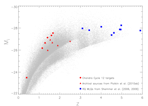
Figure 1.— SDSS absolute $i$-band magnitude, $M_{i}$, plotted versus redshift, $z$. The red filled circles and triangles show our sample of low-redshift WLQ candidates; the blue filled squares show high-redshift WLQs from Shemmer et al. (2006, 2009); the grey dots represent the 105,783 objects in the SDSS DR7 quasar catalog (Schneider et al. 2010).

Figure 2.— SDSS spectra for the 11 sources in our sample of low-redshift WLQ candidates, ordered by $\Delta\alpha_{\rm ox}$ (see §4 for definition). The $\Delta\alpha_{\rm ox}$ values and their error bars (if the source is detected in X-rays) are shown for each source. The name of each source is labeled in the format of ’Jhhmm+ddmm’. The $y$-coordinates are the flux density ($F_{\lambda}$) in arbitrary linear units. The tick marks on the $y$-axis show the zero flux-density level for each normalized spectrum. The spectra have been smoothed using a 5-pixel sliding-box filter. The spectrum of the radio-quiet BL Lac candidate J1109+3736 is shown separately in the lower right panel for convenience of presentation (since its redshift is much lower than those of the other sources in our sample). Emission lines, including C iv $\lambda$1549, C iii] $\lambda$1909, and Mg ii $\lambda$2799, are labeled in the left and upper right panels. The Mg ii $\lambda$2799, H$\beta$ $\lambda$4862, [O iii] $\lambda$5007, and H$\alpha$ $\lambda$6564 lines are labeled in the lower right panel; the Ca ii H/K break is also marked by the dotted lines. All the quoted values here are vacuum wavelengths. The spectral resolution is $R\approx$ 2000. Also included are the composite spectrum of SDSS quasars by Vanden Berk et al. (2001) and the mean spectrum of the high-redshift WLQs of Shemmer et al. (2009).

3. UV/Optical Observations

3.1. UV Emission-Line Measurements

The redshift values (see Table X-ray and Multiwavelength Insights into the Nature of Weak Emission-Line Quasars at Low Redshift) for our low-redshift WLQs are generally those from Hewett & Wild (2010) which are the best available measurements for large SDSS quasar samples. There are three sources lacking Hewett & Wild measurements. For two quasars (J1109$+$3736 and J1139$-$0201), the redshift values are taken from the catalog of Plotkin et al. (2010a). The redshift of the other source (J2115+0001; $z=2.4995\pm 0.0052$) is measured based on a Ly$\alpha$ + C iv absorption system.

To obtain accurate measurements of the weak emission lines, we manually measured rest-frame emission-line properties for C iv, Si IV, the $\lambda 1900$ complex, and Fe III UV48 (see Table 2) following the method in §2.2 of Wu et al. (2011), which is summarized below. We first smoothed the SDSS spectra with a 5-pixel sliding-box filter, and manually interpolated over strong narrow absorption regions. We then fitted a power-law local continuum for each line between their lower and upper wavelength limits $\lambda_{\rm lo}$ and $\lambda_{\rm hi}$ (see Table 2 of Vanden Berk et al. 2001). After subtracting the local continuum, we measured the REW value for each line. The C iv blueshifts were calculated between the lab wavelength in the quasar rest frame ($1549.06$ Å, see Table 2 of Vanden Berk et al. 2001) and the observed mode of all pixels with heights greater than 50% of the peak height, where mode = 3$\times$median$-2\times$mean. For comparison, we also include in Table 2 the corresponding measurements of the spectrum of PHL 1811 (Leighly et al. 2007b) and of the composite spectrum of typical SDSS quasars in Vanden Berk et al. (2001). The spectral measurements of PHL 1811 are included here because some of our low-redshift WLQ candidates show similar unusual UV/optical spectral properties to those of PHL 1811 (see §5.2). The Mg ii measurements from Shen et al. (2011) are also listed in Table 2. These measurements are reliable because the Fe ii component, which could affect the Mg ii strength measurement, was well modeled. These REW(Mg ii) values somewhat exceed the selection criterion of REW $\lesssim 5$ Å for BL Lac candidates in Plotkin et al. (2010a). This discrepancy mainly originates from differences in measurement methods. For Plotkin et al. (2010a), it was impractical to define reference wavelengths to model the continuum in a uniform way for the entire large sample since many objects lack redshift measurements. The REW values in Plotkin et al. (2010a) were measured manually after defining the continuum by eye for most sources. While this method generally performed well for BL Lac objects, it did not properly model blended Fe emission for unbeamed objects.

Only two sources (J0945+1009 and J1612+5118) have high-quality C iv coverage in their SDSS spectra so that we are able to measure their C iv REW and blueshift values. Both sources have weak and highly blueshifted C iv lines. J1139$-$0021 has no clearly detectable C iv line in its SDSS spectrum; we could only obtain an upper limit upon its REW. Therefore, we obtained follow-up UV spectroscopy for this source with the Low-Resolution Spectrograph (LRS; Hill et al. 1998) on the Hobby-Eberly Telescope (HET; Ramsey et al. 1998). The UV emission-line measurements based on the HET spectroscopy are also listed in Table 2. J1139$-$0021 has a weak and strongly blueshifted C iv line in its HET spectrum.

All of the sources having C III] coverage show weaker C III] semi-forbidden lines than those of typical quasars. The Fe III UV48 strength of our low-redshift WLQ candidates is generally similar to those of typical quasars. The SDSS spectrum of J1109+3736 does not have coverage of these rest-frame UV emission lines because of its much lower redshift, while the signal-to-noise ratio of the SDSS spectrum of J2115+0001 is too low to make reliable emission-line measurements.

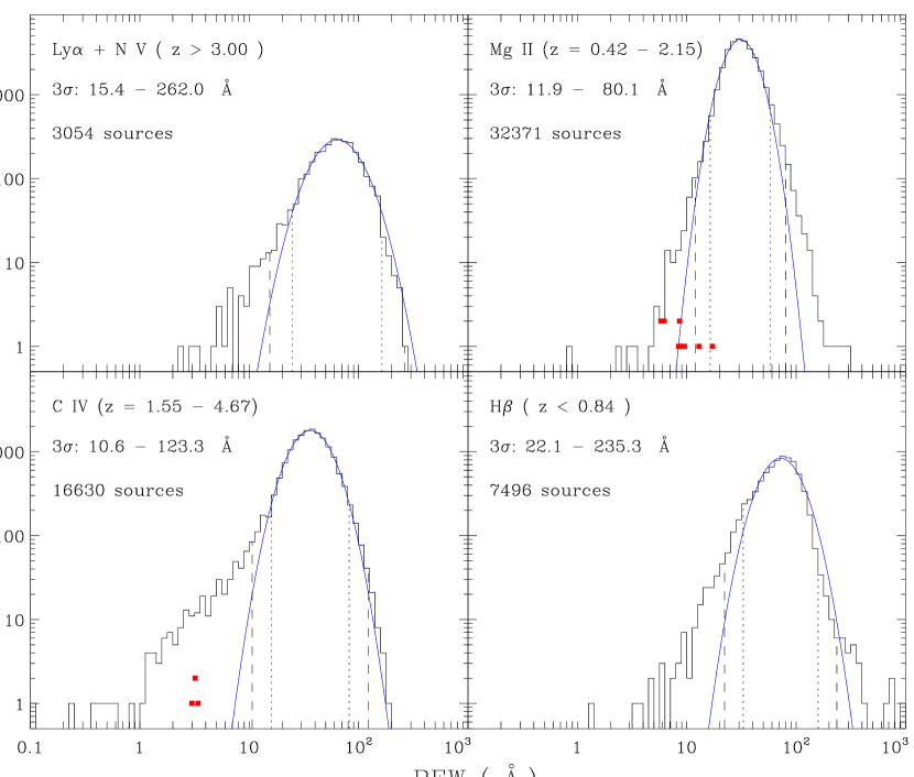
Figure 3.— Distributions of REWs of Ly$\alpha$ + N v, C iv, Mg ii, and H$\beta$ for SDSS DR7 quasar samples described in §3.2. In each panel, the blue solid line shows the best-fit lognormal distribution. The dotted and dashed lines show the 2$\sigma$ and 3$\sigma$ ranges, respectively. The 3$\sigma$ range is also noted in the upper right corner of each panel. The red filled squares with arbitrary $y$-coordinates are the REW values for our current sample. The redshift range and the number of sources for each line REW distribution are also noted.

3.2. Comparing the Emission-Line Strengths of Low-Redshift WLQ Candidates and Typical SDSS Quasars

After measuring the strengths of the UV emission lines of our low-redshift WLQ candidates (see Table 2), we further investigated the REW distributions of prominent emission lines that are covered by the SDSS spectra of low-redshift quasars (such as C iv, Mg ii, and H$\beta$). This allowed assessment of the emission-line weakness of our low-redshift, radio-quiet WLQ candidates compared to typical SDSS quasars. Furthermore, our method of selecting low-redshift WLQ candidates is different from that for high-redshift WLQs because low-redshift quasars do not have coverage of Ly$\alpha$ + N v emission in their SDSS spectra. The REW distributions of emission lines like C iv, Mg ii, or H$\beta$ may give insights on universal selection criteria for WLQ candidates at different redshifts.

We utilized the REW measurements of C iv, Mg ii, and H$\beta$ from the catalog of Shen et al. (2011) for SDSS DR7 quasars (see their Table 1). For the C iv and Mg ii lines, we adopted the REW values for the entire lines, while for H$\beta$ we added the REW values of the broad and narrow components to obtain the REW of the entire line. Shen et al. (2011) reported the REW distributions of these lines for all SDSS DR7 quasars having applicable REW measurements (see their Figs. 12–14). In this work, we selected unbiased samples of SDSS quasars with high-quality optical/UV spectra to study the REW distributions of these emission lines by imposing the following criteria:

1. We only use the DR7 quasars selected with the final algorithm given by Richards et al. (2002) to maintain consistency with DS09.

2. BAL quasars that were cataloged in Gibson et al. (2009) and Shen et al. (2011) were removed.

3. We restricted the redshift ranges of the objects for each line (C iv: $z=1.55$–$4.67$; Mg ii: $z=0.42$–$2.15$; H$\beta$: $z<0.84$) to ensure that the SDSS spectra of these objects cover the whole region of each emission line defined by $\lambda_{\rm lo}$ and $\lambda_{\rm hi}$ listed in Table 2 of Vanden Berk et al. (2001).

4. To select objects with high-quality SDSS spectra, we calculated the signal-to-noise ratio ($S/N$) of continuum regions close to each emission line, $SN_{1700}$ for C iv, $SN_{3000}$ for Mg ii, and $SN_{5150}$ for H$\beta$ (see Table 3), following the method of Gibson et al. (2009). $SN_{1700}$, $SN_{3000}$, and $SN_{5150}$ are calculated as the median of the ratio between the flux and the error (obtained from the SDSS pipeline) for all the spectral bins in the rest-frame 1650–1750 Å, 2950–3050 Å, and 5100–5200 Å regions, respectively. These wavelength regions are free of strong emission and/or absorption features, but are still close to the above emission lines in our study. We require each of the above continuum $S/N$ to be greater than 7. The $S/N$ values of the emission lines themselves were not utilized because that would introduce bias against objects with weak emission lines.

5. We eliminated the objects that have large fractions of bad pixels in their SDSS spectra in the wavelength ranges of these emission lines (these lead to unreliable measurements). We imposed the following cuts on the numbers of pixels that were included in the fitting for each line given in the catalog of Shen et al. (2011): LINE_NPIX_CIV $>250$ for C iv, LINE_NPIX_MGII $>300$ for Mg ii, and LINE_NPIX_HB $>150$ for H$\beta$.

Applying the above cuts on redshift, continuum $S/N$, and the numbers of pixels in the fitting (criteria 3–5 above) removed 35%, 27%, and 37% of the objects in the REW distribution investigations for C iv, Mg ii, and H$\beta$, respectively. All the above restrictions and quality cuts are necessary because unreliable line measurements could significantly affect the REW distributions particularly in the tails with low or high REW values.

Fig. 3 shows the REW distributions of the C iv, Mg ii, and H$\beta$ lines for our selected samples of SDSS quasars. We also include the histogram for Ly$\alpha$ + N v from DS09 for comparison. DS09 also showed a histogram for C iv REWs of SDSS DR5 quasars, which has a similar profile as the C iv REW histogram in Fig. 3. We fit the REW histogram of each line with a lognormal distribution (see the blue solid lines in Fig. 3; also see the dotted and dashed lines for the $2\sigma$ and $3\sigma$ ranges of each lognormal model). The REW measurements for the quasars in our low-redshift WLQ sample (see §3.1) are also shown in Fig. 3. All the C iv REW values of our sources are far below the negative 3$\sigma$ deviation of the lognormal distribution. Most of the REW(Mg ii) values are also below the negative 3$\sigma$ deviation of the lognormal distribution; the largest REW(Mg ii) value for our sample is close to the negative 2$\sigma$ deviation (see the top right panel of Fig. 3).

The REW distribution of Ly$\alpha$ + N v in DS09 shows a prominent tail toward low REW values; this tail is the basis on which the high-redshift WLQs are defined. The C iv REW distribution shows similar behavior in that a more prominent skew tail toward low REW values exists, while there is no corresponding tail toward high REW values. However, the histogram of the Mg ii REWs appears more symmetric, with only small tails toward both the low end and high end of the REW distribution. The H$\beta$ REW distribution is similar to that for Ly$\alpha$ + N v; a prominent tail toward low REW values exists, while the tail toward high REW values is much less significant. We randomly chose sets of sources in the tails with low or high REW values in the histograms for C iv, Mg ii, and H$\beta$ and then visually examined their SDSS spectra and the quality assessment plots for their individual spectral fits in Shen et al. (2011). These sources have good spectral-fit quality; their REW measurements should be reliable. It is worth noting that the quasars in the REW histograms for various lines have different ranges of redshift and luminosity, which may affect their REW distributions (e.g., via the Baldwin effect; Baldwin 1977). We test this hypothesis by comparing the C iv and Mg ii REW distributions for a set of SDSS quasars with $1.55\;<\;z\;<\;2.15$ and $45\;<\;\log\nu L_{3000}\;<\;46$ ($\nu L_{3000}$ is the luminosity at rest-frame 3000 Å in erg s^-1, obtained from Shen et al. 2011). Fig. 4 shows that both the C iv and Mg ii REW distributions show similar behavior to the distributions presented in Fig 3; the C iv histogram has a significant tail at the low REW end, while the Mg ii histogram is symmetric with weak tails. While the physical reason for the different emission-line REW distributions is unclear, the Mg ii line has low optical depth, while the C iv line has much higher optical depth (e.g., see Eracleous et al. 2009). In the context of a disk-wind model for the BELR (e.g., Murray & Chiang 1997; Proga et al. 2000), the C iv emission is considered to be mainly from the AGN wind, while the Mg ii line mostly originates from the accretion disk (e.g., Leighly 2004; Richards et al. 2011).

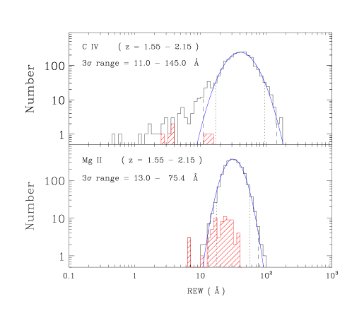
Figure 4.— Distributions of REWs for C iv (top panel) and Mg ii (bottom panel) for the same set of SDSS quasars with $1.55\;<\;z\;<\;2.15$ and $45\;<\;\log L_{3000}\;<\;46$. The red shaded histogram in the top panel shows the REW(C iv) distribution for sources with REW(Mg ii) below the 3$\sigma$ negative deviation for Mg ii. The red shaded histogram in the bottom panel shows the REW(Mg ii) distribution for sources with REW(C iv) below the 3$\sigma$ negative deviation for C iv. The bottom panel shows that many objects with weak C iv emission do not have weak Mg ii. Other lines follow the same definitions as those in Fig. 3.

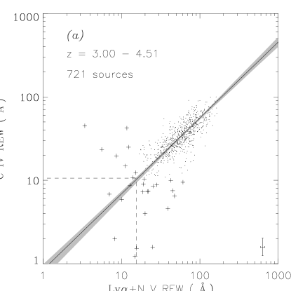
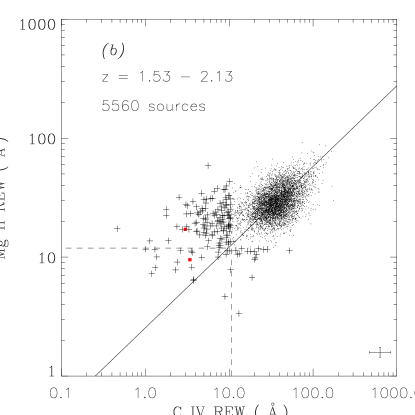
Figure 5.— Correlations between line REWs: $(a)$ Ly$\alpha$ vs. C iv; $(b)$ C iv vs. Mg ii; $(c)$ Mg ii vs. H$\beta$. No upper limits are present for any REW measurements. The median errors of the REW measurements for sources with the corresponding weak emission line (i.e., REW values below the $3\sigma$ negative deviation) are shown in the lower right corner of each panel. The solid lines show the best-fit power-law models. The dashed lines show the 3$\sigma$ values of the weak REW tails in Fig. 3. The red filled squares show the sources in our current sample. The crosses in each panel are the sources having REW values below the negative 3$\sigma$ deviation for either of the emission lines in the panel. The grey-shaded area in panel $(a)$ shows the 90% confidence uncertainty range of the best-fit correlation. The redshift range and the total number of sources in each panel are also noted.

The $3\sigma$ tail toward low REW values of the C iv histogram is defined by REW(C iv)$\;\lesssim\;10$ Å, which is consistent with that derived in DS09. Using this criterion one could perhaps hope to extend the redshift range of WLQ selection from $z\;>3$ down to $z\;>1.5$. However, this definition of WLQs has significant inconsistency with that in DS09 based on REW(Ly$\alpha$ + N v)$\;<\;15.4$ Å. Fig. 5$(a)$ shows the relation between the REW values of Ly$\alpha$ + N v and C iv, and the best-fit power-law model found using the IDL routine linmix_err. The shaded area shows the 90% confidence uncertainty range obtained via a nonparametric bootstrap method (Efron 1979). Although the REW values of these two lines are positively correlated, large scatter exists. Over half of the sources with REW(Ly$\alpha$ + N v)$\;<\;15.4$ Å have REW(C iv)$\;>\;10$ Å, and vice versa (see Fig. 5$a$). The large scatter is likely to be intrinsic, since the REW measurement errors (see Fig. 5 for typical error bars) are much smaller than the scatter. DS09 also suggested the inconsistency between sources with weak Ly$\alpha$ + N v and those with weak C iv emission. A total of 39 of the 74 WLQs cataloged in DS09 have REW(C iv)$\;>\;10$ Å based on the measurements in Shen et al. (2011). As stated in DS09, their measurements may underestimate REW(Ly$\alpha$ + N v) when strong intervening absorption exists; this is perhaps one reason for the inconsistency. The correlation between the REWs of C iv and Mg ii also has significant scatter, and so does the correlation between the REWs of Mg ii and H$\beta$ (see Figs. 5$b$ and 5$c$). The red shaded histograms in Fig. 4 show the REW(C iv) distribution for sources with weak Mg ii and the REW(Mg ii) distribution for sources with weak C iv. While the sources with weak Mg ii also tend to have weak C iv (below the negative $2\sigma$ deviation), many objects with weak C iv have fairly strong Mg ii (see the bottom panel of Fig. 4).

Given the results above, it is therefore difficult to find consistent criteria for WLQs at different redshifts using different emission lines even though the REW distributions of C iv and H$\beta$ show similar behavior to that of Ly$\alpha$ + N v. Since there is no single line that is covered by SDSS spectroscopy for quasars at all redshifts between zero and six, it appears that there is not a straightforward, direct way to define universal selection criteria for WLQs at all redshifts solely based on SDSS spectroscopy. Therefore, we only choose our low-redshift WLQ candidates mainly from the catalog of Plotkin et al. (2010a), which has a strict criterion on all emission-line strengths (REW $\lesssim 5$ Å). Future UV spectroscopy which covers the Ly$\alpha$ + N v and/or the C iv regions for low-redshift WLQs will provide insights toward a universal definition for WLQs.

4. X-ray Data Analysis

The six new low-redshift WLQ candidates targeted in Chandra Cycle 12 were observed with the S3 CCD of the Advanced CCD Imaging Spectrometer (ACIS; Garmire et al. 2003). The reduction of the Chandra data was performed using standard CIAO v4.3 routines. X-ray images were produced for the observed-frame soft (0.5–2.0 keV), hard (2.0–8.0 keV), and full (0.5–8.0 keV) bands using ASCA grade 0, 2, 3, 4, and 6 events. The wavdetect algorithm (Freeman et al. 2002) was run on the images using a detection threshold of $10^{-5}$ and wavelet scales of $1$, $\sqrt{2}$, $2$, $2\sqrt{2}$, and $4$ pixels. All targets, except J0945$+$1009, were detected by Chandra within $0.8^{\prime\prime}$ of the optical coordinates. The X-ray images of J0945$+$1009 were visually examined, and no hint of a detection was found. Aperture photometry was performed using the IDL aper procedure on each object. An aperture radius of $1.5^{\prime\prime}$ was adopted for each source ($\approx 95\%$ enclosed energy for soft band, $\approx 90\%$ enclosed energy for hard band; aperture corrections were applied) except J1109$+$3736 and J1530$+$2310, for which the aperture radius was $3.0^{\prime\prime}$ because of their large numbers of detected X-ray counts (see Table 4; no aperture corrections were applied to these two sources). The background region for each source was defined as an annulus with inner and outer radii of twice and three times the aperture radius. All background regions are free of X-ray sources. The upper limits upon X-ray counts for J0945+1009 were determined using the method of Kraft et al. (1991) at 95% confidence. Table 4 lists the X-ray counts in the three bands, as well as the band ratio (defined as the ratio between hard-band counts and soft-band counts) and effective power-law photon index for each source. The effective power-law photon index was determined from the band ratio using the Chandra PIMMS tool, under the assumption of a power-law model with Galactic absorption only.

Four archival sources (J1139$-$0201, J1604$+$4326, J2115$+$0001, and J2324$+$1443) were observed by Chandra in Cycles 5, 7, and 10. All of the quasars were detected by Chandra except J2115$+$0001. Similar Chandra data-reduction and processing procedures were performed for these objects. Three of them (J1139$-$0201, J2115$+$0001, and J2324$+$1443) were targeted in their Chandra observations, for which the aperture radius was set to be $1.5^{\prime\prime}$. J1604$+$4326 was serendipitously covered by the ACIS-I detector in two Chandra observations. We measured the X-ray counts individually for these two observations, and then calculated the mean count rate and flux in the soft band. This source did not show significant variability ($\lesssim 12\%$) between its two Chandra observations ($\approx 10$ hours apart in the quasar rest frame). The aperture radius ($2.6^{\prime\prime}$) for this source was determined to be the 95% enclosed-energy radius at $1.497$ keV based on the point spread function (PSF) of the ACIS detector at an off-axis angle of $3.7^{\prime}$. The Chandra observations of J2115$+$0001 and J2324$+$1443 were briefly reported in Plotkin et al. (2010b), and our results are consistent with theirs.

One archival source (J1013$+$4927) was serendipitously covered by XMM-Newton on 2004 April 23. Data reduction and processing were performed using standard XMM-Newton Science Analysis System (v10.0.0) routines. This source is undetected by both the MOS and pn detectors using the eboxdetect procedure. Visual inspection of the images verifies the non-detection of this source. We only used the data from the MOS detectors because they have higher angular resolution, which enables more reliable count extraction and background estimation. The events files were filtered by removing background flaring periods (12% of the total exposure time) in which the count rate exceeded $0.35$ s^-1 for events with energies above 10 keV. The aperture for photometry ($49.9^{\prime\prime}$ radius) was taken to be the 90% enclosed-energy radius at $1.5$ keV based on the PSF of the MOS detectors at an off-axis angle of $6.4^{\prime}$. The upper limits upon X-ray counts were determined to be $3\sqrt{N}$, where $N$ is the total counts within the aperture.

Table 5 lists the key X-ray, optical, and radio properties of our low-redshift WLQs:

Column (1): The SDSS equatorial coordinates (J2000) for the source.

Column (2): The apparent $i$-band magnitude of the source using the SDSS quasar catalog BEST photometry.

Column (3): The absolute $i$-band magnitude for the source, $M_{i}$, from the SDSS DR7 quasar catalog (Schneider et al. 2010), calculated by correcting for Galactic extinction and assuming a power-law spectral index of $\alpha_{\nu}\;=\;-0.5$ (e.g., Vanden Berk et al. 2001).

Column (4): The Galactic neutral hydrogen column density in units of $10^{20}$ cm^-2, obtained with the Chandra COLDEN tool.

Column (5): The count rate in the observed-frame soft X-ray band ($0.5$–$2.0$ keV), in units of $10^{-3}$ s^-1. For the two off-axis sources (J1013+4927 and J1604+4326), the count rate (or upper limit) is corrected for vignetting using exposure maps.

Column (6): The Galactic absorption-corrected flux in the observed-frame soft X-ray band in units of $10^{-14}$ erg cm^-2 s^-1, obtained with the Chandra PIMMS tool. An absorbed power-law model was utilized with a photon index $\Gamma=2$, which is typical for quasars, and the Galactic neutral hydrogen column density for each source ($N_{H}$, given in Column 4).

Column (7): The Galactic absorption-corrected flux density at rest-frame 2 keV in units of $10^{-32}$ erg cm^-2 s^-1 Hz^-1, obtained with the Chandra PIMMS tool.

Column (8): The logarithm of the quasar X-ray luminosity in the rest-frame $2$–$10$ keV band corrected for Galactic absorption.

Column (9): The continuum flux density at rest-frame 2500 Å  in units of $10^{-27}$ erg cm^-2 s^-1 Hz^-1, from the SDSS quasar spectral property catalog in Shen et al. (2011).

Column (10): The logarithm of the monochromatic luminosity at rest-frame 2500 Å, derived from the flux density at rest-frame 2500 Å. A cosmological bandpass correction is utilized.

Column (11): The X-ray-to-optical power-law slope, given by

$$\alpha_{\rm ox}=\frac{{\rm log}(f_{\rm 2\;keV}/f_{2500\mbox{\rm~{}\scriptsize\AA}})}{{\rm log}(\nu_{\rm 2\;keV}/\nu_{2500\mbox{\rm~{}\scriptsize\AA}})}=0.384\ {\rm log}\bigg{(}\frac{f_{\rm 2\;keV}}{f_{2500\mbox{\rm~{}\scriptsize\AA}}}\bigg{)}.$$ (1)

The flux density is measured per unit frequency.

Column (12): $\Delta\alpha_{\rm ox}$, a parameter assessing the relative X-ray brightness (see §5.1), defined as

$$\Delta\alpha_{\rm ox}=\alpha_{\rm ox(measured)}-\alpha_{\rm ox(expected)}.$$ (2)

The expected $\alpha_{\rm ox}$ for a typical radio-quiet quasar is calculated using the $\alpha_{\rm ox}$-$L_{2500\mbox{\rm~{}\scriptsize\AA}}$ correlation given as Equation (3) of Just et al. (2007). The statistical significance of $\Delta\alpha_{\rm ox}$ (given in parentheses) is in units of $\sigma$, which is obtained from Table 5 of Steffen et al. (2006) as the RMS for $\alpha_{\rm ox}$ of quasars with several ranges of luminosity.

Column (13): The factor of X-ray weakness, derived from the $\Delta\alpha_{\rm ox}$ values in Column (12), quantifying the X-ray weakness of our sources compared to a typical radio-quiet quasar with similar UV/optical luminosity, calculated as $f_{\rm x-weak}=10^{-\Delta\alpha_{\rm ox}/0.384}\approx 403^{-\Delta\alpha_{\rm ox}}$. A source with $\Delta\alpha_{\rm ox}$$=-0.384$ has an X-ray flux only $\approx 10\%$ that of typical quasars, corresponding to an X-ray weakness factor of $\approx 10$.

Column (14): The optical-to-radio power-law slope, given by

$$\alpha_{\rm ro}=\frac{{\rm log}(f_{\rm 5\;GHz}/f_{2500\mbox{\rm~{}\scriptsize\AA}})}{{\rm log}(\nu_{\rm 5\;GHz}/\nu_{2500\mbox{\rm~{}\scriptsize\AA}})}.$$ (3)

The values of $f_{2500\mbox{\rm~{}\scriptsize\AA}}$ are given in Column (9). The values of $f_{5\;{\rm GHz}}$ were calculated using a radio power-law slope of $\alpha_{\nu}$ = $-0.8$ (e.g., Falcke et al. 1996; Barvainis et al. 2005) and a flux at an observed-frame wavelength of 20 cm, $f_{20\;{\rm cm}}$. For sources detected by the FIRST survey (Faint Images of the Radio Sky at Twenty-Centimeters; Becker et al. 1995), $f_{20\;{\rm cm}}$ was taken from the FIRST source catalog. For sources covered but not detected by the FIRST survey, the upper limits for radio flux density were placed as $f_{20\;{\rm cm}}<0.25+(5\sigma_{\rm rms})$ mJy, where $\sigma_{\rm rms}$ is the RMS noise of the FIRST survey at the object’s coordinates (see §5.3.1 of Plotkin et al. 2010a for more details). For the two sources not covered by the FIRST survey (J2115+0001 and J2324+1443), the radio flux density was measured via targeted VLA observations (see §3.1 of Plotkin et al. 2010b).

The $\alpha_{\rm ro}$ parameter is related to the commonly used radio-loudness parameter, $R=f_{5\;{\rm GHz}}/f_{4400\mbox{\rm~{}\scriptsize\AA}}$ (e.g., Kellermann et al. 1989), by the following equation:

$$\alpha_{\rm ro}=\frac{{\rm log}[R(2500/4400)^{\alpha_{\nu}}]}{{\rm log}(\nu_{\rm 5\;GHz}/\nu_{2500\mbox{\rm~{}\scriptsize\AA}})}=-0.186\;{\rm log}\;R-0.023,$$ (4)

where we use $\alpha_{\nu}=-0.5$. Therefore, we have $\alpha_{\rm ro}$$>-0.21$ for radio-quiet quasars ($R<10$); $-0.39<\;$$\alpha_{\rm ro}$$<-0.21$ for radio-intermediate quasars ($10<R<100$); and $\alpha_{\rm ro}$$<-0.39$ for radio-loud quasars ($R>100$). All the low-redshift WLQ candidates in our sample are radio quiet. Note that the radio and optical observations of our sources are non-simultaneous. While the non-simultaneity does not generally alter the classification of typical radio-quiet quasars, it may significantly affect that of BL Lac objects because of their rapid and large-amplitude variability.

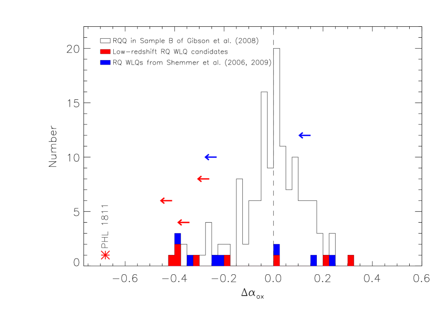
Figure 6.— Distribution of $\Delta\alpha_{\rm ox}$ values for the WLQ candidates, compared to that of the 132 radio-quiet, non-BAL quasars in Sample B of Gibson et al. (2008). The red histograms and red leftward arrows represent the low-redshift sources in our sample which are detected (8 sources) and undetected (3 sources) in X-rays, respectively. The blue histogram and blue leftward arrows represent the high-redshift sources from Shemmer et al. (2006, 2009) which are detected (7 sources) and undetected (2 sources) in X-rays, respectively. The unshaded histogram shows the radio-quiet, non-BAL quasars in Sample B of Gibson et al. (2008). PHL 1811 is shown as a red asterisk. The dashed vertical line shows $\Delta\alpha_{\rm ox}$$=0$. Note the many ($>50\%$) WLQs with $\Delta\alpha_{\rm ox}$$\;<-0.2$.

5. Results and Discussion

5.1. Relative X-ray Brightness

The $\Delta\alpha_{\rm ox}$ parameter (see Eqn. 2 for definition) is utilized to assess the X-ray brightness of a quasar relative to typical radio-quiet quasars with similar UV luminosity. We compare the $\Delta\alpha_{\rm ox}$ distribution of our low-redshift, radio-quiet WLQ candidates (see Fig. 6) to that of the 132 radio-quiet, non-BAL quasars in Sample B of Gibson et al. (2008), which represent typical radio-quiet SDSS quasars. All of the 132 Sample B quasars are X-ray detected. The Peto-Prentice test (e.g., Latta 1981), implemented in the Astronomy Survival Analysis package (ASURV; e.g., Lavalley et al. 1992), is used to assess whether our low-redshift WLQ candidates follow the same $\Delta\alpha_{\rm ox}$ distribution as that for typical quasars (see results in Table 6). We prefer the Peto-Prentice test to other possible similar tests because it is the least affected by the factors of different censoring patterns or unequal sizes of the two samples which exist in our case. We also compare the $\Delta\alpha_{\rm ox}$ distribution of high-redshift, radio-quiet WLQs in Shemmer et al. (2006, 2009) to that of our low-redshift, radio-quiet WLQ candidates and that of typical SDSS quasars (also see Fig. 6 and Table 6).

The $\Delta\alpha_{\rm ox}$ distribution of our low-redshift, radio-quiet WLQ candidates is significantly different from that of typical SDSS quasars. The probability of null-hypothesis (two samples following the same distribution) is only $6.3\times 10^{-7}$. This result is mainly due to the presence of a skew tail of X-ray weak WLQs (see Fig. 6). Seven out of the 11 objects in our sample of low-redshift, radio-quiet WLQ candidates have $\Delta\alpha_{\rm ox}$$\;<-0.2$, giving a fraction of X-ray weak objects of ($64^{+34}_{-24}$)% (68% confidence level). The mean $\Delta\alpha_{\rm ox}$ value for the low-redshift, radio-quiet WLQ candidates is $-0.214\pm 0.078$, calculated with the Kaplan-Meier estimator also implemented in the ASURV package, while that for the Sample B quasars is $-0.001\pm 0.011$. The $\Delta\alpha_{\rm ox}$ distribution of the nine high-redshift, radio-quiet WLQs in Shemmer et al. (2006, 2009) is also different from that of typical radio-quiet SDSS quasars, but less significantly (the probability of null-hypothesis is $7.1\times 10^{-3}$). Five of the nine objects in the high-redshift, radio-quiet WLQ sample have $\Delta\alpha_{\rm ox}$$\;<\;-0.2$, giving a fraction of X-ray weak objects of ($56^{+37}_{-24}$)% (68% confidence level); we note that the fraction could be somewhat higher (6/9) owing to the weak X-ray upper limit for J1237+6301. The mean $\Delta\alpha_{\rm ox}$ value for the high-redshift, radio-quiet WLQs is $-0.144\pm 0.075$. As expected the combined low-redshift and high-redshift, radio-quiet WLQ sample (mean $\Delta\alpha_{\rm ox}$ value of $-0.187\pm 0.056$) also follows a different $\Delta\alpha_{\rm ox}$ distribution from that of typical SDSS quasars (null-hypothesis probability of $4.5\times 10^{-6}$). The $\Delta\alpha_{\rm ox}$ distribution of low-redshift, radio-quiet WLQ candidates is consistent with that of high-redshift, radio-quiet WLQs (null-hypothesis probability of 0.35), though the sample sizes being compared are limited.

5.2. Classifying Radio-Quiet WLQs

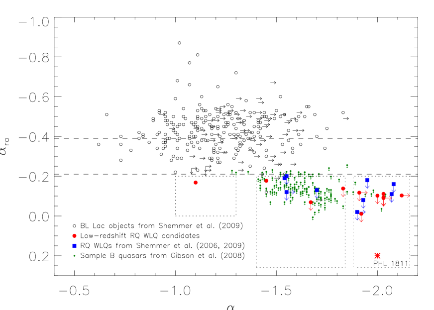
Figure 7.— $\alpha_{\rm ro}$–$\alpha_{\rm ox}$ diagram for WLQ candidates (red filled circles for low-redshift objects in our sample; blue filled squares for high-redshift objects in Shemmer et al. 2006, 2009), BL Lac objects (black open circles; Shemmer et al. 2009), and typical radio-quiet SDSS quasars (small green dots; Sample B quasars of Gibson et al. 2008). The red asterisk represents PHL 1811. Rightward (downward) pointing arrows represent $\alpha_{\rm ox}$ ($\alpha_{\rm ro}$) upper limits. The two dashed lines mark the criteria for radio-quiet ($\alpha_{\rm ro}$$>-0.21$), radio-intermediate ($-0.39<$$\alpha_{\rm ro}$$<-0.21$), and radio-loud ($\alpha_{\rm ro}$$<-0.39$) objects. The boxes bordered by dotted lines show the three suggested groups of WLQ candidates based on their multi-band properties. Note that the WLQ sample has an excess of objects with large negative $\alpha_{\rm ox}$ values, compared to both typical radio-quiet quasars and BL Lac objects.

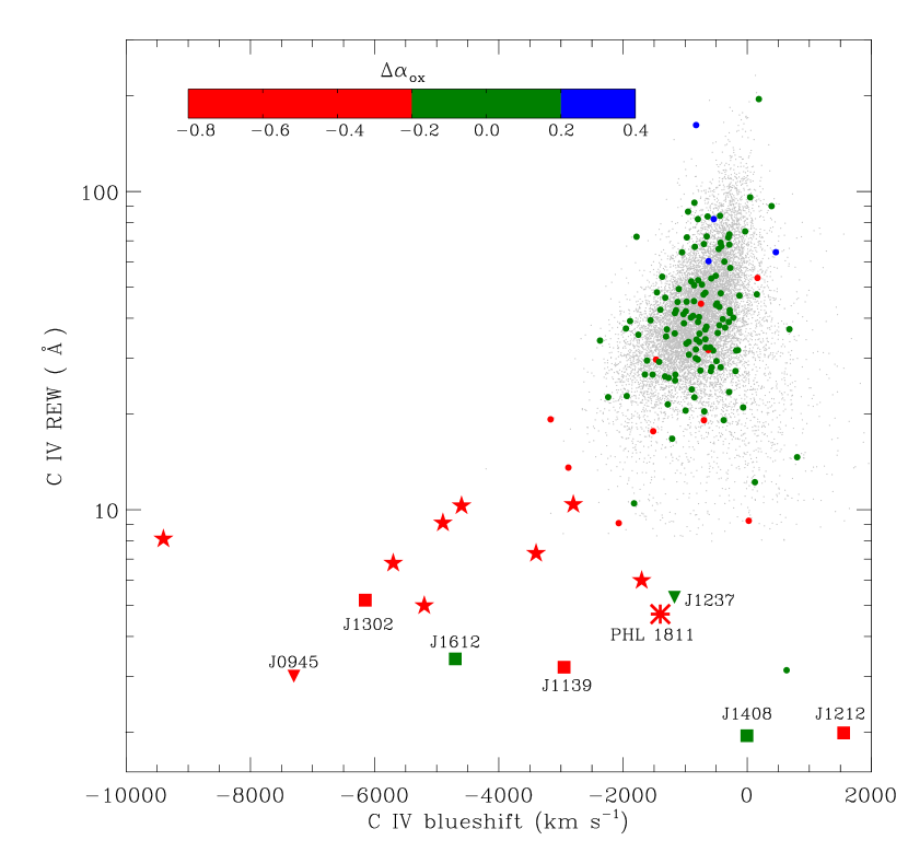
Figure 8.— REW(C iv) plotted against the C iv blueshift for our radio-quiet WLQ candidates (filled squares for X-ray detected sources, filled upside-down triangles for X-ray undetected sources), PHL 1811 (asterisk), radio-quiet PHL 1811 analogs in Wu et al. (2011) (stars), and radio-quiet, non-BAL quasars in Sample B of Gibson et al. (2008a) (circles). These sources are color-coded according to their $\Delta\alpha_{\rm ox}$ values (three color bins are used, corresponding to the X-ray weak, X-ray normal and X-ray strong sources described in §5.2, respectively). The color bar shows the $\Delta\alpha_{\rm ox}$ range for each color. Source names for WLQs are labeled in the format of ’J$hhmm$’ for brevity. The grey dots show the 13,582 radio-quiet quasars in Sample A of Richards et al. (2011; see their Fig. 7).

To investigate the multi-band properties of low-redshift, radio-quiet WLQ candidates, we plotted the sources of our sample in an $\alpha_{\rm ro}$-$\alpha_{\rm ox}$ diagram (Fig. 7) along with the high-redshift, radio-quiet WLQs in Shemmer et al. (2006, 2009), the BL Lac sample in Shemmer et al. (2009), and the Sample B quasar in Gibson et al. (2008). The low-redshift, radio-quiet WLQ candidates have similar multi-band properties to those of high-redshift, radio-quiet WLQs. They are generally much fainter in radio and X-rays than most of the BL Lac objects. The weak emission lines of low-redshift, radio-quiet WLQ candidates are therefore not likely due to the dilution by relativistically boosted continua as for BL Lac objects (see discussion in §4.1 of Shemmer et al. 2009). However, it is possible that a small percentage of the WLQ candidates actually belong to the radio-faint tail of the BL Lac population (see below).

The population of radio-quiet WLQ candidates (both at low redshift and high redshift) has a wide dispersion of relative X-ray brightness and UV emission-line properties. Motivated by their $\Delta\alpha_{\rm ox}$ distribution, their emission-line properties discussed below, and observations of related objects (e.g., Wu et al. 2011), we will discuss them in three groups.

The majority of WLQ candidates are not only X-ray weaker than BL Lac objects, but also weaker than typical radio-quiet SDSS quasars. These WLQ candidates may belong to the notable class of X-ray weak quasars termed “PHL 1811 analogs” which were recently studied in detail by Wu et al. (2011). The PHL 1811 analogs generally have weak and highly blueshifted high-ionization lines (e.g., C iv, Si iv), weak semi-forbidden lines (e.g., C iii]), and strong UV Fe ii and/or Fe iii emission. Some of our low-redshift, radio-quiet WLQs have similar UV emission-line properties to those of PHL 1811, as listed below:

1. J0812+5225 ($\Delta\alpha_{\rm ox}$$=-0.42$) has weak C iii] and strong Fe ii emission.

2. J0945+1009 ($\Delta\alpha_{\rm ox}$$\;<\;-0.34$) has weak C iv and C iii] emission lines. Its C iv line is highly blueshifted ($\approx-7000$ km s^-1).

3. J1252+2640 ($\Delta\alpha_{\rm ox}$$=-0.39$) has weak C iii] and strong Fe ii emission.

4. J1139$-$0201 ($\Delta\alpha_{\rm ox}$$=-0.38$) has weak and highly blueshifted ($\approx-2950$ km s^-1) C iv emission, weak C iii] emission, and strong Fe iii emission.

A high-redshift, radio-quiet WLQ J1302+0030 ($\Delta\alpha_{\rm ox}$$=-0.38$) also has a weak and highly blueshifted C iv emission line (DS09; Wu et al. 2011). All of the above mentioned sources are X-ray weak by a factor of $>\;7$ (see Table 5). Fig. 8 shows the distribution of our WLQ candidates in the $\Delta\alpha_{\rm ox}$$-$C IV blueshift$-$ REW(C IV) parameter space. J0945+1009, J1139$-$0201 and J1302+0030 are similar to PHL 1811 analogs in this diagram. Based on the model in §4.6 of Wu et al. (2011), these PHL 1811 analogs may have high-ionization shielding gas with large column density and a large covering factor of the BELR which blocks most of the ionizing photons, resulting in weak high-ionization emission lines. If a quasar of this kind is viewed through the BELR and shielding gas, it would be an X-ray weak WLQ with weak and highly blueshifted high-ionization lines (e.g., C iv). Based on the estimate in §4.6 of Wu et al. (2011), PHL 1811 analogs should make up $\approx 30\%$ of the total WLQ population. However, our sample of low-redshift, radio-quiet WLQ candidates appears to have a higher fraction ($\gtrsim 50\%$) of PHL 1811 analogs, which may indicate our sample has some selection bias toward X-ray weak WLQ candidates. This bias could perhaps be the result of a more strict criterion upon the strengths of emission lines for most sources in our sample (REW $\lesssim$ 5 Å). Quasars with weaker emission lines (e.g., C iv) are perhaps more likely to be weak in X-rays (e.g., see §4.5 of Wu et al. 2011). The apparently higher fraction of PHL 1811 analogs in our sample than that in Wu et al. (2011) may perhaps also be caused simply by small-sample statistics. A Fisher’s exact test (Fisher 1922) gives an $11.1\%$ probability for the different fractions of PHL 1811 analogs among these two samples under the null hypothesis (i.e., the two samples have the same fraction of PHL 1811 analogs).

Some of our WLQ candidates have similar X-ray brightness to that of typical radio-quiet quasars ($-0.2\lesssim$ $\Delta\alpha_{\rm ox}$ $\lesssim 0.2$). Their high-ionization lines are also weak, but perhaps not highly blueshifted (e.g., see Fig. 8 for J1408+0205). Some of them (e.g., J1612+5118) have very weak UV Fe ii and/or Fe iii emission. J1612+5118 does seem to have a highly blueshifted C iv line, for which the reason is unclear. However, the C iv line of this source is close to the blue border of its SDSS spectral coverage. Further UV spectroscopy with better C iv coverage is needed to confirm its C iv blueshift. Based on the model in Wu et al. (2011), these sources are similar to PHL 1811 analogs physically, but they are viewed at different orientations. These sources are observed along lines of sight that avoid the shielding gas and the BELR. Therefore they appear normal in X-rays. Their high-ionization lines are generally not highly blueshifted.

In our WLQ candidate sample, one source (J1109+3736) is remarkably strong in X-rays. It also shows similar UV/optical spectral properties to those of BL Lac objects. This source may belong to the radio-faint tail of the BL Lac population; we will discuss it further in §5.5. It is worth noting that the division of our radio-quiet WLQ candidates into the three groups discussed above (as shown in Fig. 7) is somewhat arbitrary. We do have some “border-line” sources with $\Delta\alpha_{\rm ox}$$\;\approx\;\pm 0.2$ (e.g., J1212+5341). It is difficult to classify these sources clearly based on current information.

5.3. The Infrared-to-X-ray SEDs of the Radio-Quiet WLQ Candidates

Figure 9.— Rest-frame spectral energy distributions (SEDs) of our low-redshift WLQs with the best multiwavelength coverage, and of the radio-quiet BL Lac candidate J1109+3736, ordered by $\Delta\alpha_{\rm ox}$. The photometric data points are from WISE (open diamonds), 2MASS (open triangles), SDSS (filled circles), GALEX (open circles), and X-ray observations (asterisks). The average SED of all SDSS quasars from the sample of Richards et al. (2006) is also shown (solid curve), scaled to the flux at rest-frame $10^{15}$ Hz. A parabolic SED for typical BL Lac objects is shown by the dotted line in the top-left panel. The ‘+’ signs in the bottom right-panel show the POSS photometry for J1109+3736.

For the purpose of investigating further the multi-wavelength SEDs of our low-redshift, radio-quiet WLQs, we gathered photometry for our sample from the following bands: (1) near- and mid-infrared from WISE (The Wide-field Infrared Survey Explorer; Wright et al. 2010); (2) near-infrared from 2MASS (The Two Micron All Sky Survey; Skrutskie et al. 2006); (3) optical from the SDSS; (4) UV from GALEX (The Galaxy Evolution Explorer; Martin et al. 2005); and (5) X-rays from this work. Fig. 9 shows the SEDs of the five low-redshift WLQs in our sample which have the best multi-band coverage. We also include the SED of the radio-quiet BL Lac candidate J1109+3736 (see more discussion in §5.5). A key point to keep in mind is that these multi-band observations are non-simultaneous. The SEDs are therefore subject to potential distortions due to variability.

We examined the WISE and GALEX image tiles by eye to identify potential cases of source blending, confusion, or incorrect matching caused by the low angular resolution of WISE and GALEX. None of the sources in our sample is subject to these kinds of problems. The 2MASS magnitudes in the SDSS DR7 quasar catalog were utilized; this catalog provided aperture photometry for additional sources detected down to $2\sigma$ (see §5 of Schneider et al. 2010). For the sources without detections at $\geq 2\sigma$, we adopted flux upper limits obtained following the same photometry procedure (C. M. Krawczyk & G. T. Richards 2011, private communication). The first five sources in Fig. 9 are from the groups of X-ray weak and X-ray normal WLQ candidates discussed above. Their mid-infrared-to-UV SEDs are generally consistent with the composite SEDs of typical SDSS quasars in Richards et al. (2006), and they are significantly different from the SEDs of BL Lac objects (see the dotted parabolic line in the top-left panel of Fig. 9; e.g., Nieppola et al. 2006). We also investigated the SEDs for the WISE-covered radio-quiet objects cataloged in Plotkin et al. (2010a) which do not have sensitive X-ray coverage (see the Appendix). The majority of them also have mid-infrared-to-UV SEDs consistent with those of typical radio-quiet quasars. Lane et al. (2011) obtained similar results for their high-redshift WLQs; the composite SED of their high-redshift WLQs is inconsistent with SEDs of BL Lac objects. For one source in our sample, J0945+1009, the flux in the UV band is lower than for typical SDSS quasars (see the GALEX data points in the top-right panel of Fig. 9). The UV deficiency of this source may be caused by Ly$\alpha$-forest intervening absorption. However, Laor & Davis (2011) argued that such intervening absorption is not significant ($\sim 11\%$ at most) for this source with $z=1.66$. The near-infrared-to-UV SED of J0945+1009 can be well fitted with their local black-body model for a cold accretion disk.

5.4. X-ray Spectral Properties of Low-Redshift WLQ Candidates

Most of the low-redshift, radio-quiet WLQ candidates do not have sufficient X-ray counts for an individual X-ray spectral analysis. We therefore investigate the average X-ray spectral properties for these sources via stacking analyses and joint fitting.

A stacked spectral analysis was performed for the six low-redshift, radio-quiet WLQ candidates with $\Delta\alpha_{\rm ox}$$\;<\;-0.3$ (J0812+5225, J0945+1009, J1139$-$0201, J1252+2640, J2115+0001, and J2324+1443). These sources are the weakest in X-rays among the full sample of low-redshift WLQ candidates. The detected sources have similar numbers of X-ray counts, so that any one of them will not dominate the stacking analysis. These six sources span a relatively wide range of redshift ($z=1.15$–$2.50$), and thus the observed-frame bands of each source correspond to different energy ranges in the rest frame. However, under the assumption of a simple power-law spectral model, one can stack the X-ray counts to obtain the average effective power-law photon index. We added the X-ray counts of these sources in the observed-frame soft band and hard band, respectively. The numbers of total net counts are $14.4^{+4.9}_{-3.7}$ in the soft band and $5.2^{+3.4}_{-2.2}$ in the hard band ($68\%$ confidence level), and the resulting band ratio is $0.36^{+0.27}_{-0.18}$. With the average Galactic neutral hydrogen column density of these sources ($N_{\rm H}=3.50\times 10^{20}$ cm^-2), the band ratio was converted to an effective power-law photon index $\Gamma=1.66^{+0.63}_{-0.51}$. The average X-ray spectrum of the X-ray weak low-redshift WLQs is perhaps somewhat harder than that for typical radio-quiet quasars ($\Gamma\approx 2$), but it is consistent within the error bars. This average X-ray spectrum is likely softer than that of the PHL 1811 analogs at $z=2.19$–$2.38$ ($\Gamma=1.10^{+0.45}_{-0.40}$) in Wu et al. (2011) which was also obtained via a stacking analysis, but consistent within 2$\sigma$. Both stacking analyses suffer from large uncertainty due to limited X-ray counts. For a sample combining the six X-ray weak WLQs analyzed here (which are likely to be PHL 1811 analogs) and the radio-quiet PHL 1811 analogs in Wu et al. (2011), the average X-ray spectrum has a flat effective power-law photon index of $\Gamma=1.35^{+0.33}_{-0.31}$. Deeper X-ray observations are necessary to give tighter constraints on the X-ray spectral properties of these X-ray weak WLQ candidates.

Two sources (J0945+1009 and J2115+0001) are undetected by Chandra. Adding the X-ray counts of these two sources cannot generate a stacked source that would be detected by Chandra, because both of these two sources have zero X-ray counts. However, we are able to obtain a tighter average constraint on their X-ray brightness via stacking analysis. The upper limit upon the soft-band count rate of the stacked source is $2.51\times 10^{-4}$ s^-1. Average values of redshift, Galactic $N_{\rm H}$, and $f_{2500\mbox{\rm~{}\scriptsize\AA}}$ are adopted in the following calculation. The upper limit upon the average flux density at rest-frame 2 keV is $5.16\times 10^{-33}$ erg cm^-2 s^-1 Hz^-1 under the assumption of the Galactic-absorbed power law with $\Gamma=2$. The upper limits upon $\alpha_{\rm ox}$ and $\Delta\alpha_{\rm ox}$ are calculated to be $\alpha_{\rm ox}$ $<\;-2.21$ and $\Delta\alpha_{\rm ox}$ $<\;-0.50$. Therefore, these two sources are X-ray weak by a factor of $>\;20$ on average.

For the two X-ray normal, low-redshift WLQs (J1604+4326 and J1612+5118), we performed joint fitting to study the average X-ray spectral properties of these sources. The X-ray spectra were extracted from apertures of $3^{\prime\prime}$ radius centered on the X-ray positions of these sources via the standard CIAO routine psextract. The background spectra were extracted from annular regions with inner radii of $6^{\prime\prime}$ and outer radii of $9^{\prime\prime}$, which are free of X-ray sources. Two spectra were extracted individually for J1604+4326 from its two Chandra observations. Spectral fitting was performed with XSPEC v12.6.0 (Arnaud 1996). The $C$-statistic (Cash 1979) was used in the spectral fitting instead of the standard $\chi^{2}$ statistic because the $C$-statistic is well suited to the limited X-ray counts in our analysis (e.g., Nousek & Shue 1989). We fit the spectra jointly using a power-law model with a Galactic absorption component represented by the wabs model (Morrison & McCammon 1983). We also used another model similar to the first, but adding an intrinsic (redshifted) neutral absorption component, represented by the zwabs model. Both sources were assigned their own values of redshift and Galactic neutral hydrogen column density; the Galactic column density was fixed to the values calculated with COLDEN (Column 4 of Table 5). The joint fitting results are shown in Table 7. The quoted errors or upper limits are at the 90% confidence level for one parameter of interest ($\Delta\;C=2.71$; Avni 1976; Cash 1979). The average X-ray spectral properties of these two sources are similar to those of typical radio-quiet quasars. They have an average photon index ($\Gamma=2.07^{+0.31}_{-0.30}$), consistent with that of typical radio-quiet quasars ($\Gamma\approx 2$). The average photon index is also consistent with those from their band-ratio analyses. We did not find evidence of strong intrinsic neutral absorption for J1604+4326 and J1612+5118 ($N_{\rm H}\;\lesssim\;1.58\times 10^{22}$ cm^-2); the spectral fitting quality was not improved after adding the intrinsic neutral absorption component.

Figure 10.— X-ray spectra of SDSS J1530+2310 (top panel; binned to a minimum of 10 counts per bin) and SDSS J1109+3736 (bottom panel; binned to a minimum of 20 counts per bin) fitted with a power-law model with Galactic absorption. The residuals are shown in units of $\sigma$. The inset of each panel shows contours of the photon index vs. intrinsic neutral hydrogen column density parameter space, at confidence levels of 68%, 90%, and 99%, respectively.

Two sources (J1109+3736 and J1530+2310) have sufficient X-ray counts for individual spectral analysis. We will discuss the X-ray spectral properties of J1530+2310 here and leave the radio-quiet BL Lac candidate J1109+3736 for the next subsection. The X-ray spectrum of J1530+2310 was extracted following the same procedure as for J1604+4326 and J1612+5118 (see above). The spectrum of J1530+2310 was first grouped to have at least 10 counts per bin (see Fig. 10). We used the same spectral models as those for the joint fitting above. The standard $\chi^{2}$ statistic was utilized. The fitting results are also shown in Table 7. Fig. 10 shows the X-ray spectrum, the best-fit power-law model with Galactic absorption, and the contour plot of the $\Gamma-N_{\rm H}$ parameter space for the spectral model with intrinsic neutral absorption for J1530+2310. The X-ray spectral properties of J1530+2310 are similar to those of J1604+4326 and J1612+5118. The photon index of J1530+2310 from the spectral fitting ($\Gamma=2.11^{+0.37}_{-0.34}$) is consistent with that from the band-ratio analysis (see Table 4). J1530+2310 also shows no evidence of strong intrinsic neutral absorption ($N_{\rm H}\;\lesssim\;2.67\times 10^{22}$ cm^-2). In summary, the X-ray spectral properties of X-ray normal low-redshift WLQs are consistent with those of typical radio-quiet quasars. Shemmer et al. (2009) found similar results for their high-redshift, radio-quiet WLQs. Their sources have a somewhat harder average X-ray spectrum ($\Gamma=1.86^{+0.72}_{-0.48}$), perhaps because they fit both X-ray weak and X-ray normal WLQs jointly. Shemmer et al. (2009, 2010) also performed individual X-ray spectral analysis on two high-redshift, radio-intermediate WLQs (J1141+0219 and J1231+0138).

5.5. J1109+3736: The Radio-quiet BL Lac Candidate

J1109+3736 is a radio-quiet BL Lac candidate based on its multi-band properties. It is strong in X-rays by a factor of $\approx 6.3$ ($\alpha_{\rm ox}$$\;=\;-1.10$, $\Delta\alpha_{\rm ox}$$\;=\;0.31$). Its $\alpha_{\rm ox}$ value is similar to that of the majority of the BL Lac population (see Fig. 7). X-ray spectral analysis was carried out for J1109+3736 following similar procedures as those in §5.4. The Chandra spectrum of J1109+3736 was grouped to have at least 20 counts per bin (see Fig. 10). The best-fit parameters are listed in Table 7. The X-ray spectrum, the best-fit power-law model with Galactic absorption, and $\Gamma-N_{\rm H}$ contours for J1109+3736 are also shown in Fig. 10. The best-fit photon index of J1109+3736 ($\Gamma=1.77\pm 0.14$) is consistent with that from the band-ratio analysis. This photon index value indicates a harder X-ray spectrum than those for the majority of the high-energy peaked BL Lac objects (HBL), which have a mean photon index $\Gamma\approx 2.2$, but it is still consistent with the broad distribution of HBL photon-index values (e.g., see the bottom panel of Fig. 1 in Donato et al. 2005). Although this source has a high X-ray count rate, we do not expect strong photon pile-up effects because a $1/2$ subarray mode was used for its Chandra observation. There is no evidence for significant intrinsic absorption in the J1109+3736 spectrum ($N_{\rm H}\;\lesssim\;1.4\times 10^{21}$ cm^-2).

The SDSS spectrum of J1109+3736 (see the bottom-right panel of Fig. 2) shows a strong power-law continuum without any detectable emission lines, in particular no Balmer lines. Note that some of the X-ray weak, low-redshift WLQ candidates (e.g., PHL 1811; see Leighly et al. 2007b) have fairly strong Balmer lines. The strength of its Ca ii H/K break ($C=0.185$) indicates a relatively small contribution to the SDSS spectrum from the host galaxy. J1109+3736 shows moderate X-ray variability between its Chandra observation and the epoch of the ROSAT All Sky Survey in 1990 November (RASS; Voges et al. 1999). It was not detected by RASS. The upper limit for $\alpha_{\rm ox}$ is estimated to be $\alpha_{\rm ox}$$\;<\;-1.29$, showing a factor of $>3$ variation compared to its Chandra observation. The quasar should have been detected in the RASS if it had the same X-ray brightness as that in the Chandra epoch (expecting $\approx 20$ counts in a 250 s RASS observation). There is also evidence for optical variability of J1109+3736. This source was optically identified during the Cambridge APM (Automated Plate Measuring Machine) scans of POSS (Palomar Observatory Sky Survey) plates (e.g., McMahon et al. 2002). We converted the APM magnitudes in the $O$ and $E$ bands ($O=20.76,\;E=19.12$) into a $B$-band magnitude ($B=20.57$) using Equations (1–3) in McMahon et al. (2002). We also converted the SDSS magnitudes to a $B$-band magnitude ($B=18.88$) using the equations in Table 1 of Jester et al. (2005). The $B$-band magnitude difference is 1.69, indicating a factor of $\sim 5$ variability over a time span of $\sim 50$ years. This source shows greater variability than most quasars during this time span (e.g., see Fig. 24 of Sesar et al. 2006). Therefore, J1109+3736 is a BL Lac candidate on the radio-faint tail of the full BL Lac population.

The broad-band SED of J1109+3736 is shown in Fig. 9. It is relatively weak in the near infrared compared to its SDSS brightness. However, the SED profile of this source could be strongly affected by its variability (see the comparison between its SDSS and POSS fluxes in Fig. 9) given its possible BL Lac nature. Infrared photometry from WISE, which will be available in the WISE full data release, will be helpful because the infrared-to-UV SEDs of BL Lac objects are very different from those of typical quasars (e.g., Lane et al. 2011). Future polarization measurements of J1109+3736 will also be useful in understanding its nature, since BL Lac objects are usually highly polarized in the optical/UV band. However, polarimetry surveys of optically selected BL Lac samples (e.g., Smith et al. 2007; Heidt & Nilsson 2011) did not find any highly polarized radio-quiet BL Lac candidates, indicating this kind of source, if it indeed exists, should make up only a small fraction of the total population of radio-quiet WLQ candidates.

6. Summary and Future Studies

We have compiled a sample of 11 radio-quiet WLQ candidates with $z=0.4$–$2.5$ and presented their X-ray and multiwavelength properties. These sources are mainly selected from the catalog of radio-quiet, weak-featured SDSS quasars in Plotkin et al. (2010a). Six of them were observed in new Chandra Cycle 12 observations, while five have archival Chandra or XMM-Newton coverage. Our main results are summarized as follows:

1. All newly observed low-redshift, radio-quiet WLQ candidates are detected by Chandra, except for J0945+1009. Three sources (J0812+5225, J0945+1009, and J1252+2640) are X-ray weak by factors of $\gtrsim\;$8–12 compared to typical quasars with similar optical/UV luminosity. Two sources (J1530+2310 and J1612+5118) are X-ray normal, while the other one (J1109+3736) is X-ray strong by a factor of 6.3. See §4.

2. Three (J1139$-$0201, J1604+4326, and J2324+1443) of the five low-redshift, radio-quiet WLQ candidates with sensitive archival X-ray coverage are detected in X-rays, while two (J1013+4927 and J2115+0001) do not have X-ray detections. All of the five archival sources are X-ray weak by factors of $\gtrsim\;$3–12. See §4.

3. The distribution of relative X-ray brightness for our low-redshift, radio-quiet WLQ candidates is significantly different from that of typical radio-quiet quasars. Our sample has a highly statistically significant excess of X-ray weak sources. About 64% (7/11) of the low-redshift, radio-quiet WLQs and about 56% (5/9) of the high-redshift, radio-quiet WLQs are X-ray weak. The X-ray weakness that is commonly found within WLQ samples may well be the driver of the weak broad-line emission. Therefore, X-ray weakness provides an important clue for understanding the nature of WLQs. See §5.1.

4. The X-ray weak sources ($\Delta\alpha_{\rm ox}$$<-0.2$) in our low-redshift WLQ sample are likely to be PHL 1811 analogs (see Wu et al. 2011). Some of them show similar UV emission-line properties to those of PHL 1811 (weak and highly blueshifted high-ionization lines, weak semi-forbidden lines, and strong UV Fe emission). A stacking analysis of these sources indicates the average effective power-law photon index to be $\Gamma=1.66^{+0.63}_{-0.51}$ (68% confidence level). See §5.2 and §5.4.

5. Sources with $-0.2\lesssim$ $\Delta\alpha_{\rm ox}$ $\lesssim 0.2$ have multi-band properties that suggest they are X-ray normal WLQs. They also have weak high-ionization lines, while some of them do not have highly blueshifted high-ionization lines. Some X-ray normal sources in our sample have weak UV Fe emission. The average X-ray spectral properties of these sources are similar to those of typical SDSS quasars. According to the unification model in §4.6 of Wu et al. (2011), these sources may have a similar geometry and physical nature to the PHL 1811 analogs, but with different viewing angles. See §5.2 and §5.4.

6. The mid-infrared-to-UV SEDs of the X-ray weak and X-ray normal low-redshift WLQ candidates are generally consistent with the composite SEDs of typical SDSS quasars, suggesting that these sources are not likely to be BL Lac objects with relativistically boosted continua and diluted emission lines. See §5.3.

7. The X-ray strong source J1109+3736 ($\Delta\alpha_{\rm ox}$$>0.3$) may be a radio-quiet BL Lac object. It has similar X-ray brightness ($\alpha_{\rm ox}$$=-1.10$) to those of typical BL Lac objects. The SDSS spectrum of J1109+3736 shows a similar continuum to those of BL Lac objects. It also has shown moderate X-ray (a factor of $>3$) and optical (a factor of $\approx 5$) variability in comparisons with archival data. A Chandra spectral analysis using a Galactic-absorbed power-law model gives $\Gamma=1.77\pm 0.14$; thus its X-ray spectrum is harder than those of the majority of high-energy peaked BL Lac objects. There is no evidence of significant intrinsic X-ray absorption for this source. See §5.5.

Future studies of larger samples of radio-quiet WLQ candidates will be helpful to clarify their nature. UV spectroscopy covering the Ly$\alpha$ + N v and C iv regions of low-redshift, radio-quiet objects is necessary to study the REW distributions of these two lines, and their REW correlations. This will provide insights toward a possible universal definition for WLQs at all redshifts, which should enable systematic studies of larger, unbiased, and more complete samples of WLQ candidates. For current WLQ studies, it is difficult to perform reliable mid-infrared-to-X-ray SED and correlation analyses because of the limited sample size. Further accumulation of high-quality X-ray data will substantially enlarge the sample sizes for such analyses. Deeper X-ray observations are required to convert the X-ray flux upper limits into detections and thus to study the true overall distribution of relative X-ray brightness for radio-quiet WLQ candidates. High-quality X-ray spectroscopy should be able to reveal any X-ray absorbers in X-ray weak WLQ candidates, clarifying the cause of their X-ray weakness and the geometry of these quasars. More accurate measurements of the photon indices of their hard X-ray power-law spectra can better constrain the $L/L_{\rm Edd}$ values of WLQ candidates (e.g., Shemmer et al. 2008) to see whether extremely high/low $L/L_{\rm Edd}$ is the physical cause of their weak broad emission lines. Therefore, radio-quiet WLQ candidates will be excellent targets of future missions with much higher X-ray spectroscopic capability, e.g., the Advanced Telescope for High Energy Astrophysics (ATHENA). Near-infrared spectroscopy covering the H$\beta$ region of the low-redshift WLQ candidates will also allow estimation of their $L/L_{\rm Edd}$ values (e.g., Shemmer et al. 2010).

Although most WLQ candidates likely do not have relativistically boosted continua, this work suggests that a minority of them may belong to the radio-faint tail of the BL Lac population. Further growth of the high-quality multiwavelength database, especially in the infrared band, is crucial to study the broad-band SEDs of WLQ candidates, which could distinguish BL Lac objects from WLQs (see §5.5). Full release of the WISE source catalog will greatly benefit SED studies of radio-quiet WLQ candidates. BL Lac objects often have large-amplitude variability and high polarization in the UV/optical band. Long-term UV/optical monitoring and polarimetry of X-ray strong WLQ candidates will help to identify their nature conclusively.

Appendix A Spectral Energy Distributions of Additional Radio-Quiet WLQ Candidates

The broad-band SEDs of WLQ candidates are able to provide useful insights into their nature. Lane et al. (2011) showed that the mid-infrared-to-UV SEDs of their high-redshift WLQs were consistent with those of typical quasars, but were significantly different from those of typical BL Lac objects. In §5.3 we have obtained similar results for the X-ray weak and X-ray normal WLQ candidates in our low-redshift sample (see Fig. 9). However, it is possible to gain insights from SED measurements even when sensitive X-ray data are not available. Therefore, in this appendix we will further study the mid-infrared-to-UV SEDs of the radio-quiet weak-featured AGNs cataloged in Plotkin et al. (2010a) that do not have sensitive X-ray coverage.

We cross-correlated the objects in Table 6 of Plotkin et al. (2010a) to the WISE source catalog in its preliminary data release, obtaining 30 WISE-detected sources (not including the four sources already discussed in §5.3). The WISE coverage of the remaining sources was checked with the online image tile look-up tool. An additional six sources with WISE coverage were identified. Among these six sources, two (J0901+3846 and J1409$-$0000) were identified as stars based on their SDSS spectra and proper-motion data; these two sources were removed from our SED study. For the remaining four sources, we examined their WISE image tiles. Two of them (J0755+3525 and J1448+2407) have WISE detections in all four bands that lie below the catalog limit. We performed aperture photometry (using a standard $8.25^{\prime\prime}$ aperture radius) and obtained their fluxes by scaling their counts in the aperture to those of nearby sources (within $60^{\prime\prime}$ separation) appearing in the WISE catalog. The other two sources (J0857+2342 and J1541+2631) were not detected in their WISE images. Following the standard WISE photometry procedure, we calculated their flux upper limits at a 95% confidence level by adding the aperture flux measurement plus two times the uncertainty. For J0857+2342, we could only obtain a flux upper limit in the $w3$ band, because there are nearby bright sources in its aperture in the other band images. The photometric data in the other near-infrared-to-UV wavebands were obtained following the same methods described in §5.3. The X-ray flux limits from the ROSAT All Sky Survey are taken from Table 8 of Plotkin et al. (2010a).

The SEDs of the 34 objects are shown in Fig. A1. The majority of these sources have SEDs consistent with those of typical radio-quiet quasars in Richards et al. (2006), showing they are more likely to be WLQs in nature rather than BL Lac objects. However, there are also several sources with other kinds of SED profiles, which we discuss in more detail below.

J0834+5112, J1556+3854, J1610+3039, and J1658+6118 — These four sources have very red SEDs (strong in the infrared and weak in the optical/UV). They also have very red SDSS spectra. They are more likely to be absorbed quasars than bona fide WLQs.

J1421+0522 — This source has an SED profile peaking in the near-infrared band, which is more similar to the SEDs of BL Lac objects.

J1522+4137 — The SED of this source appears similar to that of J0945+1009, which can be fit with a cold accretion disk model as in Laor & Davis (2009). It is probably a high-redshift, radio-quiet WLQ.

J1633+4227 — The SED of this source peaks in the near-infrared band and drops rapidly in both blueward and redward directions. This SED profile is similar to that of a radio-loud BL Lac object with significant host-galaxy contamination (e.g., J0823+1524 in Plotkin et al. 2011). J1633+4227 also has the same Ca ii H/K break value ($C=0.33$) as that of J0823+1524. It is possible that J1633+4227 is a radio-quiet BL Lac object with substantial host-galaxy contamination, although its radio-loudness needs to be constrained more tightly (currently $\alpha_{\rm ro}$$>\;-0.19$ estimated from its FIRST coverage). The near-infrared peak of the SED of J1633+4227 could also perhaps be caused by extreme variability.

Figure A1.— Spectral energy distributions (SEDs) of additional radio-quiet WLQ candidates in Plotkin et al. (2010a) with WISE coverage. All the lines and symbols follow the same definitions as in Fig. 9. The $y$-axis is in arbitrary units. All the SEDs are in the rest frame, except those for the two sources without redshift information (J1541+2631 and J1556+3854) which are plotted in the observed frame.

Figure A1.— Continued.

Figure A1.— Continued.

Table 1X-ray Observation Log

			$\Delta_{{\rm Opt-X}}$	Detector	Observation	Observation	Exp. Time	Off-axis Angle
	Object Name (SDSS J)	$z$	(arcsec)		Date	ID	(ks)	(arcmin)	References
Chandra Cycle 12 Objects
	$081250.79+522530.8$	$1.153$	$0.8$	ACIS-S	2010 Dec 28	12710	$4.1$	$0.3$	1
	$094533.98+100950.1$	$1.671$	$\cdots$	ACIS-S	2011 Jan 12	12706	$3.0$	$0.3$	2
	$110938.50+373611.7$	$0.397$	$0.3$	ACIS-S	2011 Feb 27	12711	$3.1$	$0.3$	1
	$125219.47+264053.9$	$1.289$	$0.3$	ACIS-S	2011 Mar 12	12709	$3.4$	$0.3$	1
	$153044.08+231013.4$	$1.406$	$0.4$	ACIS-S	2011 Apr 15	12707	$3.0$	$0.3$	1
	$161245.68+511816.9$	$1.595$	$0.4$	ACIS-S	2011 Feb 01	12708	$3.2$	$0.3$	1
Archival X-ray Data Objects
	$101353.46+492758.1$	$1.640$	$\cdots$	MOS	2004 Apr 23	0206340201	$22.7$	$6.4$	1
	$113900.55-020140.0$	$1.903$	$0.2$	ACIS-S	2004 Jul 21	4871	$14.9$	$0.6$	1
	$160410.22+432614.6$	$1.538$	$0.2$	ACIS-I	2006 Jun 25	6933	$26.7$	$3.7$	1
			$0.2$	ACIS-I	2006 Jun 23	7343	$19.4$	$3.7$
	$211552.88+000115.5$	$2.500$	$\cdots$	ACIS-S	2008 Dec 24	10388	$9.5$	$0.3$	1,3,4
	$232428.43+144324.3$	$1.417$	$0.7$	ACIS-S	2009 May 31	10386	$5.0$	$0.3$	1,3,4

References. — (1) Plotkin et al. 2010a; (2) Hryniewicz et al. 2010; (3) Collinge et al. 2005; (4) Plotkin et al. 2010b.

Table 2Quasar UV Emission-Line Measurements

	Object Name	MJD	C iv Blueshift	REW	REW	REW	REW	REW
	(SDSS J)			(C iv)	(Si iv)	($\lambda 1900$ Å)	(Fe iii)	(Mg ii)
Chandra Cycle 12 Objects
	$081250.79+522530.8$	53297	$\cdots$	$\cdots$	$\cdots$	$3.8\pm 2.1$	$<4.5$	$8.4\pm 0.7$
	$094533.98+100950.1$	52757	$-7300\pm 1700$	$3.0\pm 1.2$	$\cdots$	$4.9\pm 1.5$	$1.7\pm 1.5$	$17.1\pm 0.8$
	$110938.50+373611.7$	53499	$\cdots$	$\cdots$	$\cdots$	$\cdots$	$\cdots$	$\cdots$
	$125219.47+264053.9$	53823	$\cdots$	$\cdots$	$\cdots$	$8.8\pm 1.2$	$2.9\pm 0.9$	$8.7\pm 0.4$
	$153044.08+231013.4$	53878	$\cdots$	$\cdots$	$\cdots$	$4.9\pm 1.5$	$2.6\pm 1.2$	$12.95\pm 0.4$
	$161245.68+511816.9$	52051	$-4700\pm 1300$	$3.4\pm 1.8$	$\cdots$	$5.1\pm 1.5$	$3.0\pm 1.5$	$9.5\pm 0.6$
Archival X-ray Data Objects
	$101353.46+492758.1$	52076	$\cdots$	$\cdots$	$\cdots$	$3.4\pm 1.8$	$<6.9$	$6.2\pm 0.8$
	$113900.55-020140.0$	52294	$\cdots$	$<9.0$	$<9.9$	$<10.8$	$<9.0$	$11.1\pm 1.1$
	$113900.55-020140.0$ (HET)	55702	$-2950\pm 1550$	$3.2\pm 2.7$	$\cdots$	$11.7\pm 1.8$	$5.5\pm 1.5$	$\cdots$
	$160410.22+432614.6$	52756	$\cdots$	$\cdots$	$\cdots$	$<1.9$	$<1.8$	$5.8\pm 1.0$
	$211552.88+000115.5$	52443	$\cdots$	$\cdots$	$\cdots$	$\cdots$	$\cdots$	$\cdots$
	$232428.43+144324.3$	52258	$\cdots$	$\cdots$	$7.6\pm 2.1$	$<5.4$	$\cdots$	$8.6\pm 0.8$
	PHL 1811	$\cdots$	$-1400\pm 250$	$4.7\pm 0.9$	$4.8\pm 0.9$	$8.3\pm 0.6$	$4.7\pm 0.6$	$\cdots$
	V01 composite	$\cdots$	$-570\pm 30$	$30.0\pm 0.3$	$8.7\pm 0.3$	$21.7\pm 0.2$	$2.9\pm 0.1$	$\cdots$

Note. — The blueshift values are in units of km s^-1. All REW values are in units of Å.

Table 3Continuum $S/N$ Values for SDSS DR7 Quasars

							$SN_{1700}$ (1650–1750 Å)					$SN_{3000}$ (2950–3050 Å)					$SN_{5150}$ (5100–5200 Å)
Object Name (SDSS J)	$m_{i}$	$z$	MJD	Plate	Fiber		$S/N$	$N_{\rm pix}$	$\lambda_{\rm lo,obs}$	$\lambda_{\rm hi,obs}$		$S/N$	$N_{\rm pix}$	$\lambda_{\rm lo,obs}$	$\lambda_{\rm hi,obs}$		$S/N$	$N_{\rm pix}$	$\lambda_{\rm lo,obs}$	$\lambda_{\rm hi,obs}$
$000006.53+003055.2$	$20.09$	$1.825$	$52203$	$685$	$467$		$4.20$	$257$	$4660$	$4943$		$2.22$	$146$	$8333$	$8616$		$0.00$	$0$	$0$	$0$
$000008.13+001634.6$	$19.49$	$1.837$	$52203$	$685$	$470$		$4.83$	$256$	$4682$	$4965$		$3.87$	$146$	$8370$	$8654$		$0.00$	$0$	$0$	$0$
$000009.26+151754.5$	$19.15$	$1.199$	$52251$	$751$	$354$		$2.30$	$57$	$3798$	$3848$		1$0.97$	$146$	$6485$	$6705$		$0.00$	$0$	$0$	$0$
$000009.38+135618.4$	$18.30$	$2.234$	$52235$	$750$	$82$		1$4.22$	$256$	$5337$	$5660$		$0.00$	$0$	$0$	$0$		$0.00$	$0$	$0$	$0$
$000009.42-102751.9$	$18.77$	$1.845$	$52143$	$650$	$199$		$9.64$	$256$	$4695$	$4979$		$5.61$	$146$	$8393$	$8678$		$0.00$	$0$	$0$	$0$

Note. — This table is available in its entirety in the online journal. Part of the table is shown here for guidance about its format.

Table 4X-ray Counts and Basic Spectral Properties

		Full Band	Soft Band	Hard Band	Band
	Object Name (SDSS J)	(0.5–8.0 keV)	(0.5–2.0 keV)	(2.0–8.0 keV)	Ratio	$\Gamma$
Chandra Cycle 12 Objects
	$081250.79+522530.8$	$3.3^{+3.0}_{-1.7}$	$3.1^{+3.0}_{-1.7}$	$<3.3$	$<1.06$	$>0.72$
	$094533.98+100950.1$	$<3.3$	$<3.2$	$<3.3$	$\cdots$	$\cdots$
	$110938.50+373611.7$	$552.3^{+24.5}_{-23.5}$	$406.4^{+21.2}_{-20.2}$	$145.8^{+13.1}_{-12.1}$	$0.36^{+0.04}_{-0.03}$	$1.68^{+0.09}_{-0.09}$
	$125219.47+264053.9$	$5.5^{+3.5}_{-2.3}$	$3.1^{+3.0}_{-1.7}$	$<7.1$	$<2.25$	$>-0.01$
	$153044.08+231013.4$	$125.8^{+12.2}_{-11.2}$	$101.9^{+11.1}_{-10.1}$	$23.9^{+6.0}_{-4.9}$	$0.23^{+0.06}_{-0.05}$	$2.12^{+0.22}_{-0.21}$
	$161245.68+511816.9$	$39.3^{+7.3}_{-6.2}$	$30.5^{+6.6}_{-5.5}$	$7.2^{+3.8}_{-2.6}$	$0.23^{+0.14}_{-0.10}$	$2.05^{+0.45}_{-0.40}$
Archival X-ray Data Objects
	$101353.46+492758.1$	$<38.6$	$<25.7$	$<28.8$	$\cdots$	$\cdots$
	$113900.55-020140.0$	$5.3^{+3.5}_{-2.2}$	$4.1^{+3.2}_{-1.9}$	$<5.1$	$<1.25$	$>0.55$
	$160410.22+432614.6$	$46.5^{+7.9}_{-6.8}$	$41.3^{+7.5}_{-6.4}$	$8.2^{+4.0}_{-2.8}$	$0.20^{+0.10}_{-0.07}$	$2.21^{+0.42}_{-0.38}$
		$31.5^{+6.7}_{-5.6}$	$26.3^{+6.2}_{-5.1}$	$<14.8$	$<0.57$	$>1.25$
	$211552.88+000115.5$	$<3.3$	$<3.2$	$<3.3$	$\cdots$	$\cdots$
	$232428.43+144324.3$	$6.4^{+3.7}_{-2.5}$	$4.1^{+3.2}_{-1.9}$	$2.1^{+2.7}_{-1.3}$	$0.52^{+0.81}_{-0.40}$	$1.38^{+1.31}_{-0.87}$

Table 5X-ray, Optical, and Radio Properties

					Count			log $L$		log $L_{\nu}$
	Object Name (SDSS J)	$m_{i}$	$M_{i}$	$N_{\rm H}$	Rate	$F_{0.5-2\;{\rm keV}}$	$f_{\rm 2\;keV}$	($2-10\;{\rm keV}$)	$f_{2500\mbox{\rm~{}\scriptsize\AA}}$	(2500 Å)	$\alpha_{\rm ox}$	$\Delta\alpha_{\rm ox}$ $(\sigma)$	$f_{\rm x-weak}$	$\alpha_{\rm ro}$
	(1)	(2)	(3)	(4)	(5)	(6)	(7)	(8)	(9)	(10)	(11)	(12)	(13)	(14)
Chandra Cycle 12 Objects
	$081250.79+522530.8$	$17.99$	$-26.18$	$4.33$	$0.76^{+0.72}_{-0.41}$	$0.34$	$1.08$	$43.48$	$2.16$	$30.88$	$-2.03$	$-0.42$ $(2.10)$	$12.43$	$>-0.093$
	$094533.98+100950.1$	$17.44$	$-27.54$	$2.90$	$<1.04$	$<0.44$	$<1.77$	$<44.00$	$3.42$	$31.39$	$<-2.03$	$<-0.34$ $(2.32)$	$>7.69$	$>-0.074$
	$110938.50+373611.7$	$18.01$	$-23.50$	$1.57$	$132.38^{+6.84}_{-6.51}$	$54.61$	$113.79$	$44.55$	$0.83$	$29.42$	$-1.10$	$0.31$ $(1.90)$	$0.16$	$-0.180$
	$125219.47+264053.9$	$17.71$	$-26.65$	$0.75$	$0.92^{+0.87}_{-0.49}$	$0.37$	$1.27$	$43.64$	$2.53$	$31.04$	$-2.03$	$-0.39$ $(2.69)$	$10.38$	$-0.109$
	$153044.08+231013.4$	$17.53$	$-27.13$	$4.23$	$35.07^{+3.75}_{-3.40}$	$15.54$	$55.76$	$45.35$	$3.32$	$31.23$	$-1.45$	$0.22$ $(1.50)$	$0.27$	$-0.184$
	$161245.68+511816.9$	$17.56$	$-27.33$	$1.66$	$9.48^{+2.05}_{-1.71}$	$3.92$	$15.17$	$44.89$	$3.34$	$31.34$	$-1.67$	$0.02$ $(0.11)$	$0.89$	$>-0.054$
Archival X-ray Data Objects
	$101353.46+492758.1$	$18.23$	$-26.68$	$0.79$	$<0.85$	$<0.44$	$<1.72$	$<43.97$	$1.59$	$31.04$	$<-1.91$	$<-0.26$ $(1.81)$	$>4.76$	$>-0.115$
	$113900.55-020140.0$	$18.88$	$-26.43$	$2.58$	$0.27^{+0.21}_{-0.13}$	$0.12$	$0.52$	$43.55$	$0.83$	$30.88$	$-2.00$	$-0.38$ $(1.91)$	$9.77$	$>-0.172$
	$160410.22+432614.6$	$17.84$	$-26.94$	$1.22$	$1.56^{+0.21}_{-0.19}$	$0.99$	$3.74$	$44.29$	$2.21$	$31.13$	$-1.83$	$-0.18$ $(1.22)$	$2.94$	$>-0.091$
	$211552.88+000115.5$	$17.84$	$-26.94$	$6.17$	$<0.33$	$<0.14$	$<0.73$	$<43.97$	$2.39$	$31.55$	$<-2.12$	$<-0.41$ $(2.78)$	$>11.70$	$-0.138$
	$232428.43+144324.3$	$19.22$	$-26.81$	$4.26$	$0.82^{+0.64}_{-0.39}$	$0.33$	$1.18$	$43.73$	$1.21$	$30.80$	$-1.92$	$-0.32$ $(1.60)$	$6.82$	$>-0.145$

Table 6Results of Peto-Prentice Tests

Sample I (No. of sources)	vs.	Sample II (No. of sources)		Statistic	Null-hypothesis Probability
Low-$z$ RQ WLQs (11)		RQ Sample B quasars (132)		$4.982$	$6.29\times 10^{-7}$
High-$z$ RQ WLQs (9)		RQ Sample B quasars (132)		$2.693$	$7.08\times 10^{-3}$
Low-$z$ + High-$z$ RQ WLQs (20)		RQ Sample B quasars (132)		$4.589$	$4.45\times 10^{-6}$
Low-$z$ RQ WLQs (11)		High-$z$ RQ WLQs (9)		$0.932$	$0.351$

Note. — See Feigelson & Nelson (1985) for the detailed definition of the test statistic. The null-hypothesis probability was calculated from each test statistic using a Gaussian distribution, e.g., $1-P_{G}=6.29\times 10^{-7}$, where $P_{G}$ is the cumulative Gaussian probability at $4.982\sigma$.

Table 7X-ray Spectral Analysis

		Power Law			Power Law
		with Galactic Absorption			with Galactic and Intrinsic Absorption
Object Name		$\Gamma$	$\chi^{2}/\nu$		$\Gamma$	$N_{H}(10^{22}\ {\rm cm}^{-2})$	$\chi^{2}/\nu$
J1109+3736		$1.77^{+0.14}_{-0.14}$	$42.09/23$		$1.79^{+0.26}_{-0.15}$	$<0.14$	$42.08/22$
J1530+2310		$2.11^{+0.37}_{-0.34}$	$14.18/9$		$2.18^{+0.97}_{-0.41}$	$<2.67$	$14.13/8$
J1604+4326 / J1612+5118		$2.07^{+0.31}_{-0.30}$	$77.38/105$		$2.10^{+0.53}_{-0.33}$	$<1.58$	$77.38/105$

References

- Abazajian et al. (2009) Abazajian, K. N., Adelman-McCarthy, J. K., Agüeros, M. A., et al. 2009, ApJS, 182, 543
- Anderson et al. (2001) Anderson, S. F., Fan, X., Richards, G. T., et al. 2001, AJ, 122, 503
- Arnaud (1996) Arnaud, K. A., 1996, in ASP Conf. Ser. 101, Astronomical Data Analysis Software and Systems V, ed. G. H. Jacoby & J. Barnes (San Francisco:ASP), 17
- Avni (1976) Avni, Y. 1976, ApJ, 210, 642
- Baldwin (1977) Baldwin, J. A. 1977, ApJ, 214, 679
- Barvainis et al. (2005) Barvainis, R., Lehár, J., Birkinshaw, M., Falcke, H., & Blundell, K. M. 2005, ApJ, 618, 108
- Becker et al. (1995) Becker, R. H., White, R. L., & Helfand, D. J., 1995, ApJ, 450, 559
- Cash (1979) Cash, W. 1979, ApJ, 228, 939
- Collinge et al. (2005) Collinge, M. J., Strauss, M. A., Hall, P. B., et al. 2005, AJ, 129, 2542
- Diamond-Stanic et al. (2009) Diamond-Stanic, A. M., Fan, X., Brandt, W. N., et al. 2009, ApJ, 699, 782
- Donato et al. (2005) Donato, D., Sambruna, R. M., & Gliozzi, M. 2005, A&A, 433, 1163
- Efron (1979) Efron, B., 1979, The Annals of Statistics, 7, 1
- Eracleous et al. (2009) Eracleous, M., Lewis, K. T., & Flohic, H. M. L. G. 2009, New A Rev., 53, 133
- Falcke et al. (1996) Falcke, H., Sherwood, W., & Patnaik, A. R. 1996, ApJ, 471, 106
- Fan et al. (1999) Fan, X., Strauss, M. A., Gunn, J. E., et al. 1999, ApJ, 526, L57
- Fan et al. (2006) Fan, X., Strauss, M. A., Richards, G. T., et al. 2006, AJ, 131, 1203
- Feigelson & Nelson (1985) Feigelson, E. D., & Nelson, P. I. 1985, ApJ, 293, 192
- Fisher (1922) Fisher, R. A. 1922, Journal of the Royal Statistical Society, 85(1), 87
- Freeman et al. (2002) Freeman, P. E., Kashyap, V., Rosner, R., & Lamb, D. Q. 2002, ApJS, 138, 185
- Garmire et al. (2003) Garmire, G. P., Bautz, M. W., Ford, P. G., Nousek, J. A., & Ricker, G. R., Jr. 2003, Proc. SPIE, 4851, 28
- Gehrels (1986) Gehrels, N. 1986, ApJ, 303, 336
- Gibson et al. (2008) Gibson, R. R., Brandt, W. N., & Schneider, D. P. 2008, ApJ, 685, 773
- Gibson et al. (2009) Gibson, R. R., Jiang, L., Brandt, W. N., et al. 2009, ApJ, 692, 758
- Heidt & Nilsson (2011) Heidt, J., & Nilsson, K. 2011, A&A, 529, A162
- Hewett & Wild (2010) Hewett, P. C., & Wild, V. 2010, MNRAS, 405, 2302
- Hill et al. (1998) Hill, G. J., Nicklas, H. E., MacQueen, P. J., et al. 1998, Proc. SPIE, 3355, 375
- Hryniewicz et al. (2010) Hryniewicz, K., Czerny, B., Nikołajuk, M., & Kuraszkiewicz, J. 2010, MNRAS, 404, 2028
- Isobe et al. (1990) Isobe, T., Feigelson, E. D., Akritas, M. G., & Babu, G. J. 1990, ApJ, 364, 104
- Jester et al. (2005) Jester, S., Schneider, D. P., Richards, G. T., et al. 2005, AJ, 130, 873
- Just et al. (2007) Just, D. W., Brandt, W. N., Shemmer, O., et al. 2007, ApJ, 665, 1004
- Kellermann et al. (1989) Kellermann, K. I., Sramek, R., Schmidt, M., Shaffer, D. B., & Green, R. 1989, AJ, 98, 1195
- Kelly (2007) Kelly, B. C. 2007, ApJ, 665, 1489
- Komatsu et al. (2009) Komatsu, E., Dunkley, J., Nolta, M. R., et al. 2009, ApJS, 180, 330
- Kraft et al. (1991) Kraft, R. P., Burrows, D. N., & Nousek, J. A. 1991, ApJ, 374, 344
- Lane et al. (2011) Lane, R. A., Shemmer, O., Diamond-Stanic, A. M., et al. 2011, ApJ, 743, 163
- Laor & Davis (2011) Laor, A., & Davis, S. W. 2011, MNRAS, 417, 681
- Latta (1981) Latta, R. B., 1981, J. Am. Stat. Assoc., 76, 713
- Lavalley et al. (1992) Lavalley, M., Isobe, T., Feigelson, E., 1992, in ASP Conf. Ser. 25, Astronomical Data Analysis Software and Systems I, ed. D. M. Worrall, C. Biemesderfer, & J. Barnes (San Francisco, CA: ASP), 245
- Leighly (2004) Leighly, K. M. 2004, ApJ, 611, 125
- Leighly et al. (2007) Leighly, K. M., Halpern, J. P., Jenkins, E. B., et al. 2007a, ApJ, 663, 103
- Leighly et al. (2007) Leighly, K. M., Halpern, J. P., Jenkins, E. B., & Casebeer, D. 2007b, ApJS, 173, 1
- Liu & Zhang (2011) Liu, Y., & Zhang, S. N. 2011, ApJ, 728, L44
- Lyons (1991) Lyons, L. 1991, Data Analysis for Physical Science Students (Cambridge: Cambridge Univ. Press)
- Londish et al. (2004) Londish, D., Heidt, J., Boyle, B. J., Croom, S. M., & Kedziora-Chudczer, L. 2004, MNRAS, 352, 903
- Martin et al. (2005) Martin, D. C., Fanson, J., Schiminovich, D., et al. 2005, ApJ, 619, L1
- McDowell et al. (1995) McDowell, J. C., Canizares, C., Elvis, M., et al. 1995, ApJ, 450, 585
- McMahon et al. (2002) McMahon, R. G., White, R. L., Helfand, D. J., & Becker, R. H. 2002, ApJS, 143, 1
- Meusinger et al. (2011) Meusinger, H., Hinze, A., & de Hoon, A. 2011, A&A, 525, A37
- Morrison & McCammon (1983) Morrison, R., & McCammon, D. 1983, ApJ, 270, 119
- Murray & Chiang (1997) Murray, N., & Chiang, J. 1997, ApJ, 474, 91
- Nestor et al. (2008) Nestor, D., Hamann, F., & Rodriguez Hidalgo, P. 2008, MNRAS, 386, 2055
- Nieppola et al. (2006) Nieppola, E., Tornikoski, M., & Valtaoja, E. 2006, A&A, 445, 441
- Nousek & Shue (1989) Nousek, J. A., & Shue, D. R. 1989, ApJ, 342, 1207
- Plotkin et al. (2010) Plotkin, R. M., Anderson, S. F., Brandt, W. N., et al. 2010a, AJ, 139, 390
- Plotkin et al. (2010) Plotkin, R. M., Anderson, S. F., Brandt, W. N., et al. 2010b, ApJ, 721, 562
- Plotkin et al. (2011) Plotkin, R. M., Anderson, S. F., Brandt, W. N., Markoff, S., Shemmer, O., & Wu, J. 2011, ApJ Letters, submitted
- Prochaska et al. (2008) Prochaska, J. X., Hennawi, J. F., & Herbert-Fort, S. 2008, ApJ, 675, 1002
- Proga et al. (2000) Proga, D., Stone, J. M., & Kallman, T. R. 2000, ApJ, 543, 686
- Ramsey et al. (1998) Ramsey, L. W., Adams, M. T., Barnes, T. G., et al. 1998, Proc. SPIE, 3352, 34
- Richards et al. (2002) Richards, G. T., Fan, X., Newberg, H. J., et al. 2002, AJ, 123, 2945
- Richards et al. (2006) Richards, G. T., Lacy, M., Storrie-Lombardi, L. J., et al. 2006, ApJS, 166, 470
- Richards et al. (2011) Richards, G. T., Kruczek, N. E., Gallagher, S. C., et al. 2011, AJ, 141, 167
- Schneider et al. (2010) Schneider, D. P., Richards, G. T., Hall, P. B., et al. 2010, AJ, 139, 2360
- Sesar et al. (2006) Sesar, B., Svilković, D., Ivezić, Ž., et al. 2006, AJ, 131, 2801
- Shemmer et al. (2006) Shemmer, O., Brandt, W. N., Schneider, D. P., et al. 2006, ApJ, 644, 86
- Shemmer et al. (2008) Shemmer, O., Brandt, W. N., Netzer, H., Maiolino, R., & Kaspi, S. 2008, ApJ, 682, 81
- Shemmer et al. (2009) Shemmer, O., Brandt, W. N., Anderson, S. F., et al. 2009, ApJ, 696, 580
- Shemmer et al. (2010) Shemmer, O., Trakhtenbrot, B., Anderson, S. F., et al. 2010, ApJ, 722, L152
- Shen et al. (2008) Shen, Y., Greene, J. E., Strauss, M. A., Richards, G. T., & Schneider, D. P. 2008, ApJ, 680, 169
- Shen et al. (2011) Shen, Y., Richards, G. T., Strauss, M. A., et al. 2011, ApJS, 194, 45
- Skrutskie et al. (2006) Skrutskie, M. F., Cutri, R. M., Stiening, R., et al. 2006, AJ, 131, 1163
- Smith et al. (2007) Smith, P. S., Williams, G. G., Schmidt, G. D., Diamond-Stanic, A. M., & Means, D. L. 2007, ApJ, 663, 118
- Steffen et al. (2006) Steffen, A. T., Strateva, I., Brandt, W. N., et al. 2006, AJ, 131, 2826
- Vanden Berk et al. (2001) Vanden Berk, D. E., Richards, G. T., Bauer, A., et al. 2001, AJ, 122, 549
- Wright et al. (2010) Wright, E. L., Eisenhardt, P. R. M., Mainzer, A. K., et al. 2010, AJ, 140, 1868
- Wu et al. (2011) Wu, J., Brandt, W. N., Hall, P. B., et al. 2011, ApJ, 736, 28
- Voges et al. (1999) Voges, W., Aschenbach, B., Boller, T., et al. 1999, A&A, 349, 389
- York et al. (2000) York, D. G., Adelman, J., Anderson, J. E., Jr., et al. 2000, AJ, 120, 1579