X-ray Emission from Optically Selected Radio-Intermediate and Radio-Loud Quasars

Abstract

We present the results of an investigation into the X-ray properties of radio-intermediate and radio-loud quasars (RIQs and RLQs, respectively). We combine large, modern optical (e.g., SDSS) and radio (e.g., FIRST) surveys with archival X-ray data from Chandra, XMM-Newton, and ROSAT to generate an optically selected sample that includes 188 RIQs and 603 RLQs. This sample is constructed independently of X-ray properties but has a high X-ray detection rate (85%); it provides broad and dense coverage of the ${\ell}-z$ plane, including at high redshifts (22% of objects have $z=2-5$), and it extends to high radio-loudness values (33% of objects have $R^{*}=3-5$, using logarithmic units). We measure the “excess” X-ray luminosity of RIQs and RLQs relative to radio-quiet quasars (RQQs) as a function of radio loudness and luminosity, and parameterize the X-ray luminosity of RIQs and RLQs both as a function of optical/UV luminosity and also as a joint function of optical/UV and radio luminosity. RIQs are only modestly X-ray bright relative to RQQs; it is only at high values of radio-loudness ($R^{*}\lower 2.0pt\hbox{$\,\buildrel\scriptstyle>\over{\scriptstyle\sim}\,$}3.5$) and radio luminosity that RLQs become strongly X-ray bright. We find no evidence for evolution in the X-ray properties of RIQs and RLQs with redshift (implying jet-linked IC/CMB emission does not contribute substantially to the nuclear X-ray continuum). Finally, we consider a model in which the nuclear X-ray emission contains both disk/corona-linked and jet-linked components and demonstrate that the X-ray jet-linked emission is likely beamed but to a lesser degree than applies to the radio jet. This model is used to investigate the increasing dominance of jet-linked X-ray emission at low inclinations.

1. Introduction

1.1. Radio-loud and radio-intermediate quasars

Quasar emission is believed to result largely from accretion onto a supermassive black hole (e.g., Lynden-Bell 1969). The bulk of the optical/UV continuum in radio-quiet quasars (RQQs) is associated with quasi-thermal emission originating in the accretion disk (e.g., Shields 1978), while the X-ray emission is postulated to arise from Compton upscattering of disk photons occuring in a hot “corona” (e.g., Haardt & Maraschi 1991). This scenario leads naturally to a correlation between optical/UV and X-ray luminosity. Extensive studies of RQQs (e.g., Avni & Tananbaum 1986; Strateva et al. 2005; Steffen et al. 2006; Just et al. 2007; Kelly et al. 2007; Green et al. 2009) have found that the optical/UV-to-X-ray spectral slope steepens (in the sense that objects become relatively less X-ray luminous) with increasing optical/UV luminosity. Intriguingly, most studies (see above references) find that there does not appear to be significant evolution with redshift in the spectral energy distributions of RQQs; despite the strong evolution in the space density of quasars, these studies generally find that RQQs in the early universe appear to have similar optical/UV-to-X-ray spectral slopes to their local analogs.

Radio-loud quasars (RLQs) are often defined to be the subset of quasars with a radio-loudness parameter satisfying $R^{*}\geq 1$, where $R^{*}$ is the logarithmic ratio of monochromatic luminosities (with units of erg s^-1 Hz^-1) measured at (rest-frame) 5 GHz and 2500 Å (e.g., Stocke et al. 1992); RQQs must minimally satisfy $R^{*}<1$ and often are found to have $R^{*}<0$. RLQs comprise $\sim$10% of quasars, with this fraction apparently varying with both luminosity and redshift (e.g., Jiang et al. 2007 and references therein). The definitive physical trigger for radio-loudness remains elusive, but RLQs generally have more massive central black holes than RQQs (e.g., Laor 2000; Metcalf & Magliocchetti 2006; also, Shankar et al. 2010 find this to be redshift-dependent), and it has also been suggested that RLQs host more rapidly spinning black holes than do RQQs (e.g., Wilson & Colbert 1995; Meier 2001; but see also Garofalo et al. 2010). RLQs and RQQs are typically treated as distinct populations, in part due to the apparent relative scarcity of objects with $R^{*}\approx 1$. The appropriateness of this canonical separation has been questioned due to the discovery of numerous quasars of intermediate radio-loudness (e.g., White et al. 2000; Cirasuolo et al. 2003), which may outnumber RLQs (e.g., White et al. 2007), but there does appear to be a genuine bimodality of $R^{*}$ allowing fairly objective distinction between RQQs and RLQs (e.g., Ivezić et al. 2004; Zamfir et al. 2008). It should be noted that RQQs are not necessarily radio-silent; for example, Miller et al. (1993) found the radio emission from radio-detected RQQs to be dominated by a starburst-linked component, and interpreted radio-intermediate quasars (RIQs) as being RQQs in which a low-power and mildly relativistic jet is viewed at low inclinations (see also, e.g., Falcke et al. 1996; Zamfir et al. 2008).

The observed properties of RLQs and their likely parent population of radio galaxies are dependent upon orientation to the observer’s line of sight (e.g., Barthel 1989; Urry & Padovani 1995). As with RQQs (e.g., Antonucci 1993), there is believed to be an obscuring “torus” present in RLQs that blocks the broad-line region from view at large inclinations, but RLQs are further complicated by significant non-isotropic jet emission. Radio jets have been measured to have relativistic bulk velocities on parsec scales from multi-epoch high-resolution radio imaging of moving knots in the inner jet, and the frequent lack of a detectable counterjet is consistent with Doppler beaming (e.g., Worrall & Birkinshaw 2006 and references therein). RLQ jets terminate in hotspots within lobes, for which the velocities are typically non-relativistic (e.g., Scheuer 1995) and so this emission is relatively isotropic. Both the ratio of radio core-to-lobe flux and the ratio of core radio-to-optical luminosities are observed to depend upon orientation, and these results suggest that both the lobe emission and the optical continuum in RLQs are correlated with intrinsic unbeamed jet power (e.g., Wills & Brotherton 1995). The luminosities of narrow emission lines appear to correlate directly with jet power, with the link plausibly coming from a mutual underlying dependence upon accretion rate and/or black-hole spin (e.g., Rawlings & Saunders 1991; Willott et al. 1999). Various unification models (e.g., Urry & Padovani 1995; Jackson & Wall 1999) link narrow-line radio galaxies, broad-line radio galaxies, RLQs, and blazars by decreasing inclination. Our focus in the present study is restricted to broad-line quasars, but our results are of potential relevance to radio galaxies and blazars in the context of such unification schemes.

X-ray studies of RLQs strongly suggest that the nuclear X-ray emission contains a significant jet-linked component. Zamorani et al. (1981) discovered that RLQs are more X-ray luminous than are RQQs with comparable optical/UV luminosities, by a typical factor of about three. Worrall et al. (1987) used Einstein data to show that the relative X-ray brightness is greater for RLQs that are more radio-luminous or have flatter radio spectra, and found no evidence for redshift evolution out to $z\sim 3.5$ in the properties of RLQs. Wilkes & Elvis (1987) and Shastri et al. (1993) uncovered X-ray spectral flattening with increasing radio loudness and radio core dominance in samples of quasars observed with Einstein. Brinkmann et al. (1997) investigated a large sample of ROSAT-detected RLQs and found that both lobe-dominated and core-dominated RLQs show X-ray luminosity correlated with core radio luminosity, with the X-ray luminosity of core-dominated RLQs increasing more rapidly with increasing core radio luminosity (e.g., their Figure 15). It is also noteworthy in the context of unification schemes that FR II (see Fanaroff & Riley 1974 for description of the FR I and FR II classes) radio-galaxy X-ray spectra typically show both a dominant absorbed and a weaker unabsorbed component, apparently linked with the disk/corona and jet, respectively (e.g., Evans et al. 2006; Hardcastle et al. 2009).

1.2. Aims of this work

Recent wide-angle, overlapping surveys in the radio (e.g., Faint Images of the Radio Sky at Twenty-cm, or FIRST; Becker et al. 1995) and optical (e.g., the Sloan Digital Sky Survey, or SDSS; York et al. 2000) may be matched (e.g., Ivezić et al. 2002) to enable the selection of large, well-defined samples of RLQs, for which X-ray properties may be investigated. For example, Suchkov et al. (2006) present a catalog of SDSS Data Release Four (DR4) quasars matched to FIRST sources as well as X-ray sources from pointed ROSAT PSPC observations. Jester et al. (2006a) matched a subset of SDSS DR5 quasars to FIRST sources and X-ray sources from the ROSAT All Sky Survey, finding radio loudness to be dependent upon both optical and X-ray luminosity. The improved capabilities of modern X-ray observatories such as Chandra and XMM-Newton have substantially advanced understanding of RLQs. For example, the high angular resolution and low background of Chandra enable the routine detection of X-ray emission from the knots of large-scale RLQ jets (e.g., Worrall 2009 and references therein), while the broad bandpass and high throughput of XMM-Newton generate high signal-to-noise X-ray spectra useful for quantifying differences between RQQs and RLQs (e.g., Page et al. 2005; Young et al. 2009) or radio galaxies and RLQs (e.g., Belsole et al. 2006). Samples of SDSS quasars with X-ray coverage by Chandra or XMM-Newton that include subsamples matched to FIRST sources are presented and discussed by Green et al. (2009) and Young et al. (2009).

Guided by the results described in $\S$1.1 (and taking advantage of our large sample size, which permits finer categorization), we consider three categories of quasars in this work: RQQs, RIQs, and RLQs (rather than just RQQs and RLQs), where we define RIQs to consist of objects with $1{\leq}R^{*}$$<2$; consequently, the objects we classify as RLQs satisfy $R^{*}\geq 2$. The goal of this study is to quantify the optical-to-X-ray properties of RIQs and RLQs and to investigate the physical origin of their X-ray emission. Such an effort requires (1) consistent selection criteria that are unbiased with respect to the X-ray properties we wish to investigate; (2) a large sample of quasars spanning a broad range of radio properties and possessing sensitive X-ray coverage; (3) radio imaging capable of resolving extended sources (multifrequency radio coverage to calculate or constrain spectral indices is also useful); (4) a high fraction of X-ray detections along with proper statistical consideration of X-ray limits; and (5) effective, broad coverage of the luminosity-redshift plane to include the full population of RIQs and RLQs, and to avoid degeneracies in regression analysis and other biases. We generate a large sample of RIQs and RLQs with archival X-ray coverage by matching the SDSS DR5 quasar catalog of Schneider et al. (2007) and the photometrically selected quasars from Richards et al. (2009) to FIRST and to high-quality observations from Chandra, XMM-Newton, or ROSAT. We supplement this primary sample with additional RLQs observed by Einstein, high-redshift RLQs, and low-luminosity RLQs detected in deep multiwavelength surveys. The full sample enables accurate parameterization of X-ray luminosity correlations across a wide range of radio properties, notably including the previously sparsely probed but well-populated RIQ regime. We are also able to take advantage of recent advances in statistical methods (e.g., Kelly 2007) in our analysis and of newly established constraints on jet properties (e.g., Mullin & Hardcastle 2009) in our modeling. In addition, our use of modern accurate cosmological parameters eliminates a source of systematic error present in some earlier analyses of luminosity correlations.

The outline of this paper is as follows: in $\S$2 we describe the selection methods used to generate our sample, in $\S$3 we discuss characteristics of the RIQs and RLQs studied here, in $\S$4 we compare the X-ray properties of RIQs and RLQs to those of RQQs, in $\S$5 we parameterize X-ray luminosity in RIQs and RLQs as a joint function of optical/UV and radio properties, in $\S$6 we determine a plausible physical model for the spectral energy distributions of RIQs and RLQs, and in $\S$7 we summarize our results. We adopt a standard cosmology with $H_{0}$ = 70 km s^-1 Mpc^-1, ${\Omega}_{M}$ = 0.3, and ${\Omega}_{\Lambda}$ = 0.7 (e.g., Spergel et al. 2007) throughout. Radio, optical/UV, and X-ray monochromatic luminosities ${\ell}_{\rm r}$, ${\ell}_{\rm uv}$, and ${\ell}_{\rm x}$ are expressed as logarithmic quantities with units of erg s^-1 Hz^-1 (suppressed hereafter), at rest-frame 5 GHz, 2500 Å, and 2 keV, respectively. In these units the radio loudness is $R^{*}={\ell}_{\rm r}-{\ell}_{\rm uv}$ and the useful quantity ${\alpha}_{\rm ox}$, the optical/UV-to-X-ray spectral slope (e.g., Avni & Tananbaum 1986), is ${\alpha}_{\rm ox}=0.384\times({\ell}_{\rm x}-{\ell}_{\rm uv})$. Object names are typically taken from the SDSS DR5 spectroscopic quasar catalog of Schneider et al. (2007) or from the SDSS DR6 photometric quasar catalog of Richards et al. (2009) and are J2000 throughout.

2. Sample selection

Our primary sample consists of 654 optically selected RIQs and RLQs with SDSS/FIRST observations and high-quality X-ray coverage from Chandra (171), XMM-Newton (202), or ROSAT (281). The primary sample is split nearly evenly between spectroscopic (312) and high-confidence photometric (342) quasars. Most (562) of the primary sample objects possess serendipitous off-axis X-ray coverage, while the remainder (92) were targeted in the observations used in our sample. The X-ray detection fraction for the primary sample is 84%; the detection fraction for those objects with Chandra/XMM-Newton/ROSAT coverage is 95%/92%/70% (typical ROSAT observations are comparatively less sensitive and have higher background). Two additional samples of spectroscopic SDSS quasars are constructed to examine the influence of SDSS targeting selection flags: a “QSO/HIZ” sample that contains 200 SDSS/FIRST RIQs and RLQs targeted as quasars from their SDSS colors (this is entirely a subsample of the spectroscopic primary sample), and a “FIRST” sample that contains 180 SDSS/FIRST RIQs and RLQs targeted as quasars based on their radio emission; there is considerable overlap between these two groups, but neither contain the quasars targeted by SDSS as “serendipitous” that we also include in the primary spectroscopic sample.

We extend the primary sample of spectroscopic/photometric RIQs and RLQs with several supplemental samples to increase coverage of the ${\ell}-z$ plane: 93 luminous RLQs with Einstein coverage from Worrall et al. (1987), 13 high-redshift RLQs studied by Bassett et al. (2004) and Lopez et al. (2006), and 31 low-luminosity RLQs selected from deep multiwavelength surveys (see $\S$2.2.3 for details and references) including the Extended Chandra Deep Field–South (E-CDF-S) and the Chandra Deep Field–South (CDF-S), the Chandra Deep Field–North (CDF-N), and the Cosmic Evolution Survey (COSMOS). These supplemental samples are combined with the primary sample to produce the full sample. Almost all analyses are performed separately on the primary sample as well as on the full sample.

The full sample consists of 791 quasars with $R^{*}\geq 1$ (with an X-ray detection fraction of 85%), of which 188 are RIQs with $R^{*}<2$ and 603 are RLQs with $R^{*}\geq 2$. The sky coverage of the full sample is shown in Figure 1. Properties for objects in the primary sample are provided in Table 1, properties for objects in the deep-fields sample are provided in Table 2, and characteristics of the various samples are provided in Table 3. In the remainder of this section, we provide details about the selection of all the samples used throughout this paper.

Figure 1.— The sky coordinates of objects in the full sample of 791 RIQs and RLQs. The filled symbols are X-ray detections, and the open symbols are X-ray upper limits. The symbol size is linearly proportional to $R^{*}$; larger symbols correspond to quasars with greater radio loudness values. Primary sample SDSS spectroscopic/photometric quasars ($n=654$) are plotted in blue/cyan, and the supplemental samples of Einstein ($n=93$) and high-redshift ($n=13$) RLQs are plotted in green and red, respectively. The deep-field sample ($n=31$) is indicated by the locations of the COSMOS, E-CDF-S, and CDF-N surveys (marked with purple squares and labels; the square size does not indicate the solid-angle coverage of these surveys).

2.1. Primary sample

2.1.1 Spectroscopic sample

The spectroscopic sample of 312 RIQs and RLQs is drawn from the SDSS DR5 Quasar Catalog of Schneider et al. (2007). The sky area covered by DR5 spectroscopic observations is 5740 deg² near the north Galactic cap (Adelman-McCarthy et al. 2007). The Schneider et al. (2007) quasar catalog includes quasars targeted for matching a variety of (often overlapping) criteria (see Schneider et al. 2007 and Richards et al. 2002 for details). Of the 77429 objects in the quasar catalog, 51577 were targeted based on quasar-like optical colors and have BEST target flags of “QSO” or “HIZ” set (see Schneider et al. 2007 for description of these parameters). Most of the remaining quasars were targeted as “serendipitous” objects based on possessing non-stellar optical colors. A smaller number of quasars were targeted based on their radio (FIRST) or X-ray (RASS) emission and/or were photometrically categorized as stars or galaxies. Quasars targeted as “QSO” or “HIZ” or “serendipitous” were considered for inclusion in the optically-selected spectroscopic sample; matching to the FIRST radio survey and then to archival high-quality X-ray coverage provides an initial list of 345 such RIQs and RLQs. As described in Appendix A, we remove from this initial list 22 BAL quasars, 8 highly reddened quasars, and 3 GHz-peaked spectrum sources. The remaining 312 objects constitute our spectroscopic sample of optically-selected RIQs and RLQs.

The radio properties of these quasars are determined from the 1.4 GHz FIRST survey, which has a resolution of $\sim$5^′′, a 5$\sigma$ limiting flux density of $\sim$1 mJy, and 9030 deg² of sky coverage, much of which overlaps the SDSS area (Becker et al. 1995). Objects were retained as RIQs or RLQs if the summed luminosity of their constituent components satisfied ${\ell}_{\rm r}>31.0$ (motivated by, e.g., Zamfir et al. 2008, who define $31<{\ell}_{\rm 1.4}<31.6$ as RIQs and ${\ell}_{\rm 1.4}>31.6$ as RLQs) along with $R^{*}>1.0$ (with ${\ell}_{\rm r}$ and $R^{*}$ defined as in $\S$1.2). Although the requirements of optical selection and a joint SDSS/FIRST detection necessarily limit the completeness of our sample, the depths of the SDSS and FIRST surveys are well matched for detecting RIQs and RLQs. An $m_{i}$=19.1 quasar (the limit for $z<3$ candidate “QSO” SDSS spectroscopic targeting) with $R^{*}=1$ and a typical spectral slopes (${\alpha}_{\rm r}=-0.5$) would have a 1.4 GHz flux density of $\simeq$0.9 mJy, near the FIRST point-source detection limit. Details of the optical screening, radio matching, and selection of X-ray observations are provided in Appendix A.

In addition to the optically-selected (“QSO/HIZ” or “serendipitous”) spectroscopic sample of 312 RIQs and RLQs, we construct and separately analyze a slightly smaller sample of 200 “QSO/HIZ” targeted spectroscopic quasars, and we also generate a sample of 180 quasi-radio-selected “FIRST” targeted spectroscopic quasars. Such objects were targeted by the SDSS on the (not necessarily exclusive) basis of being likely optical counterparts to FIRST radio sources. This does not constitute a true radio-selected sample because the SDSS retains optical magnitude limits for FIRST sources and because lobe-dominated radio sources without a FIRST core component will not be targeted by SDSS as FIRST sources, but this approach provides a useful basis for broad comparison to RIQs and RLQs targeted on the basis of their optical colors. There is considerable overlap between the categories of “QSO/HIZ” and “FIRST” targeted objects; 163 of the 180 objects (91%) with the “FIRST” flag set also have either the “QSO” or “HIZ” flags set. The median properties of these samples are similar, with median ${\Delta}(g-i)=0.06/0.08$, median ${\ell}_{\rm r}=33.14/33.16$, median $R^{*}=2.50/2.41$, and median ${\alpha}_{\rm ox}=-1.41/-1.43$ for the objects selected (as “QSO/HIZ”)/(as “FIRST”). These results do not mandate that a complete radio-selected sample of RIQs and RLQs would have properties consistent with those of color-selected SDSS RIQs and RLQs (see, e.g., McGreer et al. 2009), but they do indicate that there is substantial overlap in these selection methods.

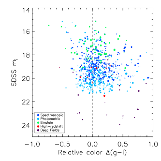
Figure 2.— Color-magnitude plot of RIQs and RLQs, where the relative color ${\Delta}(g-i)$ is the $g-i$ color (corrected for Galactic extinction) for a given object less the median quasar color at that redshift. Bluer/redder objects have negative/positive values of ${\Delta}(g-i)$. The filled symbols are X-ray detections and the open symbols are X-ray upper limits. Larger symbols correspond to more radio-loud quasars. Primary sample SDSS spectroscopic/photometric quasars are plotted in blue/cyan, and the supplemental samples of Einstein, high-redshift, and deep-field RLQs are plotted in green, red, and purple, respectively. The ${\Delta}(g-i)$ and $m_{\rm i}$ values for the deep field RLQs have been calculated by tranforming $UBVRI$ magnitudes to $ugriz$ equivalents.

2.1.2 Photometric sample

The photometric sample of 342 RIQs and RLQs is constructed from a parent population of over 1,000,000 photometric SDSS sources identified as potential quasars through the nonparametric Bayesian classification conducted by Richards et al. (2009) on unresolved SDSS DR6 objects. The efficiency of the photometric catalog at excluding non-quasar contaminants within the list of candidates is high (for example, it is estimated at 97% within a subsample of $\sim$500,000 robust UV-excess candidates; it is lower for high-redshift candidates). We consider only the most likely quasar candidates by requiring the good flag to be $\geq 1$ (this measure is determined based on several metrics; see Richards et al. 2009 for details). Our analysis requires reliable redshifts and luminosities, so we discard those sources with more uncertain photometric redshifts (probability $<0.5$ of lying within the given range). Our minimum radio loudness and radio luminosity requirements improve efficiency still further, as only a small fraction of the non-quasars in the photometric sample would be expected to display sufficient radio emission to pass these cuts; we expect that non-quasar contamination in the matched photometric SDSS/FIRST sample is negligible. By utilizing photometrically selected quasars, it is possible to expand the luminosity coverage of the primary sample. Over half of the Richards et al. (2009) catalog consists of objects fainter than $m_{\rm i}=20.1$, which is already a full magnitude fainter than the SDSS limit for spectroscopic targeting of $z<3$ “QSO” candidates (SDSS spectroscopic targeting of “HIZ” candidates is limited to objects with $m_{\rm i}\leq 20.2$). The classification scheme is calibrated with spectroscopically confirmed SDSS quasars, and consequently the optical properties of these photometrically identified quasars are expected to be consistent with those selected from the DR5 Quasar Catalog. This can be verified from Figure 2, which shows that the relative colors of the photometric RIQs and RLQs are distributed similarly to those of the spectroscopic sample, but that the photometric sample extends to fainter magnitudes.

The matching to radio sources and determination of X-ray coverage for the photometric quasars is identical to the procedure described for the spectroscopic quasars in Section 2.1.1 and Appendix A. This process produces a candidate list of 427 photometric RIQs and RLQs. However, 15 of these objects have SDSS spectroscopic redshifts obtained on an MJD of less than 53535; these objects were available for inclusion in the Schneider et al. (2007) DR5 quasar catalog but were deliberately not included therein, and are therefore not appropriate for our sample. (Recall that no known DR5 spectroscopic quasars are permitted in our photometric sample, since spectroscopic data are preferred.) After excluding objects rejected from the DR5 Schneider et al. (2007) quasar catalog, and additionally culling six GHz-peaked spectrum objects, the updated candidate list of photometric RIQs and RLQs contains 406 objects.

We perform an additional check for those RIQs and RLQs with photometric redshifts of $z_{\rm phot}\geq 1.9$ in order to improve further sample fidelity. To our knowledge, the only significant set of systematically erroneous photometric redshifts within the Richards et al. (2009) catalog, as established via cross-checking with SDSS spectroscopic data, consists of a small fraction of low-redshift ($z_{\rm spec}\leq 1$) quasars assigned photometric redshifts of $z_{\rm phot}\sim 2$. (The additional and unavoidable effect of increasing redshift uncertainty at very faint magnitudes is difficult to quantify in the absence of spectroscopic coverage, and we do not consider it here.) While such inaccuracies are atypical, it is possible to identify many of the low-redshift quasars with $z_{\rm phot}\sim 2$ through matching to UV observations carried out by the Galaxy Evolution Explorer (GALEX; Martin et al. 2005). We make use of both redshift-dependent color-color separation (D. W. Hogg 2009, personal communication) and FUV/NUV (far/near UV; $\sim$1350–1750/1750-2750 Å) band SDSS detection rates (Trammell et al. 2007) to find and discard 34 RIQs and RLQs for which the $z_{\rm phot}\sim 2$ photometric redshift is likely inaccurate (and retain another 9 for which GALEX data correctly indicates an inaccurate photometric redshift but for which we are able to use available spectroscopic redshifts). We conservatively also discard a further 25 objects with $z_{\rm phot}>1.9$ that lack GALEX coverage. Appendix B contains details of the use of GALEX data to assess the accuracy of objects with $z_{\rm phot}>1.9$. The updated candidate list of photometric RIQs and RLQs contains 347 ($=406-34-25$) objects, within which the remaining fraction with this type of redshift misidentification is only $\sim 1.5$%.

We found 82 (out of 347) photometric RIQs or RLQs with SDSS spectroscopic redshifts obtained on an MJD of greater than 53535; these objects were not available for inclusion in the Schneider et al. (2007) DR5 quasar catalog, and thus provide a “blind test” of our selection methodology above. After examination of the SDSS spectra, only two objects did not show obvious broad lines. Two non-quasar object from 82 photometric candidate RIQs and RLQs with SDSS spectra corresponds to 2.4%, suggesting that non-quasar contamination of our optical/radio matched sample is quite low, at least for brighter objects. Another three objects show BAL features. Three BAL quasars from 82 photometric RIQs and RLQs with SDSS spectra corresponds to 3.7%, suggesting that BAL contamination of our optical/radio matched sample is quite low, at least for brighter objects. This fraction is slightly lower than the typical fraction of RIQs and RLQs with BALs (e.g., Shankar et al. 2008), perhaps because the photometric color-selection is less efficient for BAL quasars with redder colors (with such a tendency reinforced by the requirement that ${\Delta}(g-i)<1$). There are then 342 ($=347-2-3$) RIQs and RLQs in the photometric sample.

The photometric redshifts for the remaining 77 photometric RIQs and RLQs with SDSS spectra were replaced with their spectroscopic redshifts. Photometric redshifts for an additional 25 photometric RIQs and RLQs were replaced with spectroscopic redshifts listed in the NASA/IPAC Extragalactic Database (NED). The ratio of the absolute value of the difference between photometric and spectroscopic redshifts to the spectroscopic redshift was checked to assess redshift accuracy. The 9 objects already identified as having substantially inaccurate photometric redshifts by the prior process of matching to GALEX data are not included in this comparison. There are only 1/7/24 objects for which this ratio exceeds 0.8/0.2/0.1, and these substantial/modest/tiny redshift errors are relatively random (the median/mean/standard-deviation of $z_{\rm phot}-z_{\rm spec}=-0.02/-0.30/0.59$ for the 24 objects with $|z_{\rm phot}-z_{\rm spec}|/z_{\rm spec}>0.1$, and $0.01/-0.08/0.33$ for all 93 objects compared). These 1/7/24 objects correspond to percentages of 1.1%/7.5%/25.8% out of the 93 redshifts checked; applying these percentages to the 240 ($=342-93-9$) photometric RIQs and RLQs lacking spectroscopic coverage suggests substantial/modest/tiny redshift errors in 0.8%/5.3%/18.1% of the full photometric sample. Not only are the percentages of errors small and relatively random, but the impact on the luminosities for objects with modestly incorrect photometric redshifts is only $\sim$0.2 (expressed in logarithmic units), less than the intrinsic scatter; this should have no appreciable impact on our analysis. The luminosities for the photometric RIQs and RLQs with SDSS spectra or NED $z_{\rm spec}$ values are recalculated using the spectroscopic redshifts. In no case did this cause the radio luminosity of a previously accepted RIQ or RLQ to drop below the minimum selection cutoff values of ${\ell}_{\rm r}=31$. Median properties of the 342 objects in the final photometric sample are presented in Table 3.

2.2. Supplemental samples

We supplement the primary sample with additional RIQs and RLQs chosen to increase coverage of the ${\ell}-z$ plane, including 93 objects previously observed by Einstein, 13 high-redshift objects (primarily targeted by Chandra), and 31 objects selected from deep-field surveys. The properties of the deep-field objects are presented in Table 2, and Table 3 includes the properties of the supplemental samples. The selection methods for these additional RIQs and RLQs are by necessity not identical to those employed to obtain our primary sample, but the optical colors of the supplemental sample RLQs are similar to those of the primary sample, as can be seen in Figure 2. The additional ${\ell}-z$ coverage provided by the supplemental samples (Figure 3) helps ensure consideration of the full population of RIQs and RLQs and also considerably reduces the ${\ell}-z$ degeneracy when performing statistical analyses below (but we conduct most fitting on both the full and primary-only samples).

2.2.1 Einstein sample

To increase population of the high-luminosity region of the ${\ell}-z$ plane, we include the RLQs with Einstein observations analyzed by Worrall et al. (1987), as this sample includes many luminous RLQs that even today do not have high-quality X-ray coverage from other observatories. Their sample of 114 RLQs includes objects from both the North and South celestial hemispheres and has an X-ray detection rate of 89%. Their sample was primarily radio-selected at both high and low frequencies and consequently includes a mix of compact and extended radio sources, and their RLQs tend to have higher radio, optical, and X-ray luminosities (and also radio-loudness values) than the objects in our primary sample. We take the radio, optical, and X-ray luminosities from Worrall et al. (1987) but translate their values to our adopted cosmology. We discard three BAL quasars, one compact steep spectrum source, and one GHz-peaked spectrum source from the Einstein sample. The relative colors of the 56 Einstein non-BAL quasars with SDSS magnitudes (of which 44 also have SDSS spectra) are plotted on Figure 2 and are similar to the relative colors of the primary sample; a Kolmogorov-Smirnov (KS) test gives a probability $p=0.36$ that the two samples are not inconsistent with arising from the same underlying distribution. Note that 3C 273 is too bright to fit on this plot, and also too bright to be targeted for spectroscopy by the SDSS. We independently find 16 objects from the full Worrall et al. (1987) sample in our primary sample (10 spectroscopic, 6 photometric) and omit these objects from the Einstein sample to avoid duplication. Many of the other Einstein objects with SDSS coverage do not appear in our primary sample for various reasons (e.g., they were targeted by SDSS based on radio rather than optical properties, or they lack FIRST coverage, or most commonly they lack recent high-quality X-ray observations). The Einstein sample is then made up of 93 RLQs. Of these, 11 were undetected by Einstein, but three of these are detected in shallow ROSAT observations, and we use these ${\ell}_{\rm x}$ measurements rather than the Einstein limits.

2.2.2 High-redshift sample

To increase population of the high-redshift region of the ${\ell}-z$ plane, we include the 15 high-redshift RIQs and RLQs tabulated by Bassett et al. (2004) and the 6 high-redshift RLQs observed by Lopez et al. (2006). These high-redshift objects were selected based on radio flux as well as redshift and were typically (15/21) targeted by Chandra in “snapshot” observations of $\sim$5 ks (6/21 were observed instead by ROSAT; all these are from Bassett et al. 2004); all are X-ray detected. The Lopez et al. (2006) objects have Southern declinations and are therefore unavailable to the SDSS/FIRST surveys. Most (11/15) of the Bassett et al. (2004) objects have SDSS coverage, and most (7/11) of these have SDSS spectra and are identified as SDSS quasars. The relative colors of the Bassett et al. (2004) RLQs for which we have SDSS magnitudes are plotted in Figure 2. One object with ${\Delta}(g-i)>1$ is discarded and not shown. We independently find 7 of the 15 objects from Bassett et al. (2004) in our primary sample and for consistency we use our measurements in our analysis of these objects. The high-redshift sample then consists of 13 ($=15-1-7+6$) objects, of which 12 are RLQs and one is an RIQ.

Some of the high-redshift RLQs have particularly large radio-loudness values, with five having $R^{*}>3.5$. These objects are referred to as “blazars” by Bassett et al. (2004) and Lopez et al. (2006) and are likely viewed at lower inclinations than most of our primary sample objects (though all of the high-redshift objects are broad-line quasars and not BL Lacs). The relatively large fraction of objects with extreme radio-loudness values within the high-redshift sample should not necessarily be taken to be representative of high-redshift RLQs.

2.2.3 Deep-fields sample

To increase population of the low-luminosity region of the ${\ell}-z$ plane, we include RIQs and RLQs identified from deep-field surveys; properties of these objects are given in Table 2. We select 16 objects by optical color (of which 14 have X-ray detections) and include a further 15 X-ray detected objects known to possess broad-line optical spectra.

We apply a color selection technique which approximates that of the primary sample when searching for lower luminosity RIQs and RLQs in deep surveys. Our general procedure is to utilize the Vanden Berk et al. (2000) color-color selection method to identify potential quasars from large catalogs of objects with $UBVRI$ photometry. This set of color cuts primarily selects for $z<2$ UV-excess objects, but also includes additional color cuts designed to identify potential quasars at higher redshift ($z=2-4$). Optical catalogs for the COSMOS region are described in Ilbert et al. (2008, 2009); for the E-CDF-S they include COMBO-17 (Wolf et al. 2004) and MUSYC (Gawiser et al. 2006); for the CDF-N they include the Hawaii survey (Capak et al. 2007). We converted $UBVRI$ to SDSS $ugriz$ magnitudes following the transformations given by Jester et al. (2005; see their Table 1) as calculated for $z\leq 2.1$ quasars and use the $ugriz$ magnitudes to calculate ${\Delta}(g-i)$ (discarding any heavily reddened objects with ${\Delta}(g-i)\lower 2.0pt\hbox{$\,\buildrel\scriptstyle>\over{\scriptstyle\sim}\,$}1$) and ${\ell}_{\rm uv}$. Accurate photometry is important for calculating colors, luminosities, and photometric redshifts, and so we additionally require $m_{\rm i}<24$ within the Chandra Deep Fields; since COSMOS has shallower X-ray coverage, we require $m_{\rm i}<22.5$ for this survey to maintain a reasonable X-ray detection fraction. These magnitude limits are factors of $\sim$90 and $\sim$20 deeper than the $m_{\rm i}<19.1$ limit for SDSS targeting of $z<3$ “QSO” objects. These optical selection criteria do not discriminate with respect to X-ray properties. The majority of the selected deep-field RIQs and RLQs have spectroscopic redshifts (see Table 2 for references), and the remainder have accurate photometric redshifts (references in Table 2) that have been derived including UV or IR data where available.

The resulting optically-selected quasar candidates are then matched to radio catalogs, and non-radio-loud objects are removed from further consideration. This step significantly improves the efficiency of the candidate list at excluding non-quasar contaminants. The COSMOS, E-CDF-S, and CDF-N surveys have highly sensitive radio coverage, with detection limits better than $\sim$50 $\mu$Jy at 1.4 GHz. The VLA 1.4 GHz radio catalogs used for the COSMOS, E-CDF-S and CDF-S, and CDF-N fields are presented in Schinnerer et al. (2007), Miller et al. (2008) [which includes many objects also given in Kellerman et al. (2008)], and Biggs & Ivison (2006), respectively. Luminous starburst galaxies make up an increasing fraction of the radio-source population at low radio fluxes and luminosities (e.g., Windhorst et al. 1985; Barger et al. 2007), and so we also impose radio-selection criteria designed to screen out starbursts. We require ${\ell}_{\rm r}>31.0$ as for the primary sample and further impose a more stringent requirement of $R^{*}>1.3$ (e.g., see Figure 8 of Barger et al. 2007) upon deep-field candidates, thereby decreasing potential starburst contamination of the sample with the tradeoff of omitting some genuine radio-intermediate deep-field quasars.

We next match to X-ray catalogs, with any X-ray limits estimated from sensitivity maps. We make use of X-ray point-source catalogs based on Chandra observations of the E-CDF-S, CDF-S, CDF-N, and COSMOS as presented in Lehmer et al. (2005), Luo et al. (2008), Alexander et al. (2003), and Elvis et al. (2009), respectively. Maximum Chandra effective exposure times are $\sim$250 ks for the E-CDF-S, $\sim$2 Ms for the CDF-S and the CDF-N, and $\sim$160 ks for COSMOS. We use a matching radius around the optical position of $2.5^{\prime\prime}$, which is large enough to account for joint uncertainties in position but sufficiently small that no spurious matches are likely (see above references).

As we are interested in characterizing the fundamental X-ray emission properties of RIQs and RLQs, it is helpful to identify and remove objects with heavy intrinsic X-ray absorption. This is important for the low-luminosity deep-field sample, since the fraction of obscured AGNs is large at low X-ray luminosities and decreases to high X-ray luminosities (from $\approx 80$% for a 2–10 keV luminosity of $10^{42}$ erg s^-1 to $\approx 20$% at $10^{45}$ erg s^-1; e.g., Hasinger 2008, and see also discussion in Brandt & Alexander 2010). Removing objects with strong optical reddening (as we do for both the primary and the deep-field samples) can also remove many objects with X-ray absorption, but for the deep-field sample we take the additional step of considering X-ray spectral shape (but not X-ray luminosity) as a selection criterion, as measured using the X-ray hardness ratio [defined as $HR=(H-S)/(H+S)$, where $H$ and $S$ are the 2–8 keV and 0.5–2 keV counts, respectively]. We screen out sources that are likely absorbed by requiring that the hardness ratio satisfy $HR<0$; this would correspond to a power-law slope of $\Gamma\simeq 1$ for no intrinsic absorption, $\simeq 2\sigma$ from the $\Gamma\simeq 1.55$ typical of RLQs (e.g., Page et al. 2005). After application of the hardness-ratio cut, this color-selection method yields 16 deep-field RIQs and RLQs, of which 14 have X-ray detections; 9 are from the E-CDF-S, 4 from the CDF-N, and 3 from COSMOS. In Appendix C, we briefly comment on interesting aspects of some of these RIQs and RLQs. Most (12/16) of the deep-field quasars selected in this manner are RLQs with $R^{*}>2$.

In addition to the color selection, we also employ optical spectra for selection, accepting RIQs or RLQs which are known to have broad emission-line spectra. Optical spectroscopy specifically targeting X-ray sources is available in the CDF-S (based on 1 Ms sources; Giacconi et al. 2002), the CDF-N (based on 2 Ms sources; Alexander et al. 2003), and COSMOS (based on XMM-Newton detections; Cappelluti et al. 2009), and is presented in Szokoly et al. (2004), Barger et al. (2003) as well as Trouille et al. (2008), and Trump et al. (2009), respectively. We include 15 RIQs and RLQs selected based on broad-line emission. Of these, one is from the CDF-N and two are from the CDF-S; these three objects have radio luminosities of ${\ell}_{\rm r}<31$ and so were not available for consideration as color-selected objects, but they do satisfy the Vanden Berk et al. (2000) color-color selection method for quasar candidates, as well as the hardness ratio cut, and so would otherwise have been expected to be selected through this process. The remaining 12 RIQs and RLQs are from the XMM-Newton COSMOS survey, which is shallower than the Chandra COSMOS survey but covers a wider area; many of these broad-line objects do not fall within the Chandra coverage and/or have radio luminosities of ${\ell}_{\rm r}<31$, and so were not considered for color selection. Again, all of these broad-line objects would have been identified as quasar candidates based on their optical colors, and all further satisfy the hardness ratio cut.

In principle this manner of selecting broad-line objects known to be X-ray sources might introduce a bias toward X-ray bright sources, were similarly optically-bright broad-line objects with X-ray limits not also considered. However, we are unaware of any broad-line objects present in the extensive optical surveys of the E-CDF-S or CDF-N which lack X-ray detections, and in any event the RIQs and RLQs selected based on optical spectroscopy could generally have had lower X-ray counts by factors of $\sim$10 and still been detected, suggesting that their relative X-ray brightness is not atypical for their optical/UV luminosities. This is supported by the observation that the ${\alpha}_{\rm ox}$ values of the broad-line selected objects are similar to those of the color-selected objects.

The complete deep-field sample then consists of 31 RIQs and RLQs, of which 29 are X-ray detected. Of these, 16 were selected by optical color (of which 14 have X-ray detections) and 15 were selected based on possessing broad-line optical spectra.

3. Sample characteristics

Characteristics of the various samples are presented in Tables 3 and 4 and illustrated in Figures 1–6. The sky coverage of the full sample is indicated in Figure 1, a color-magnitude diagram is provided as Figure 2, the redshift distribution is plotted versus optical/UV luminosities in Figure 3 and versus X-ray luminosities in Figure 4, the radio characteristics of the primary sample are given in Figure 5, and the optical/UV-to-X-ray spectral slope as a function of optical/UV luminosity is shown in Figure 6.

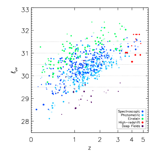
Figure 3.— Sample coverage of the ${\ell}_{\rm uv}-z$ plane, with optical/UV luminosity as measured at rest-frame 2500 Å. The filled symbols are X-ray detections, and the open symbols are X-ray upper limits. Larger symbols correspond to more radio-loud quasars. Primary sample SDSS spectroscopic/photometric quasars are plotted in blue/cyan, and supplemental sample Einstein/high-redshift/deep fields RLQs are plotted in green/red/purple. The dotted lines define luminosity bins within which various properties are summarized in Table 4.

3.1. Optical/UV luminosities

Optical/UV monochromatic luminosities for all primary sample objects are calculated at rest-frame 2500 Å from SDSS photometric $ugriz$ PSF magnitudes (corrected for Galactic extinction) via comparison to a redshifted unobscured composite quasar spectrum taken from Vanden Berk et al. (2001). This method accounts (in a statistical sense) for the flux from emission lines as well as typical breaks in the continuum slope. The error in this method due to differences in emission-line strength or spectral shape in a particular object is expected to be less than the inherent uncertainty ($\sim$30%; e.g., Vanden Berk et al. 2004; Kaspi et al. 2007) due to typical quasar optical variability. Only the AGN power-law component is included in the luminosity; a typical iron-emission “bump” near 2500 Å (e.g., Wills et al. 1985; Vanden Berk et al. 2001) is subtracted, as is the contribution from a typical RLQ host galaxy (${\ell}_{\rm uv}=28.2$ based on an old stellar population as in, e.g., Coleman et al. 1980). We verify the accuracy of this approach through comparison to $\sim$100 RQQs for which Strateva et al. (2005) calculated luminosities by fitting SDSS spectra (after dereddening and correcting for fiber inefficiencies, and also subtracting host-galaxy emission) and find close agreement (mean difference of ${\ell}_{\rm uv}-{\ell}_{\rm uv,s}=-0.03$ with a standard deviation of 0.12). By using photometric rather than spectroscopic data to compute optical/UV luminosities, we can treat the SDSS spectroscopic and photometric samples in a consistent fashion.

Optical/UV luminosities for the Einstein RLQs are taken from Worrall et al. (1987), corrected to our adopted cosmology. Optical/UV luminosities for the high-redshift RLQs are taken from Bassett et al. (2004) and Lopez et al. (2006). Optical/UV luminosities for the deep field objects are calculated from SDSS $ugriz$ equivalents, determined as described in $\S$2.2.3. The full sample (Figure 3) achieves dense coverage of the ${\ell}-z$ plane, a wide span (almost five decades) in luminosity coverage ($\sim$2.5 decades at a given redshift even without considering deep-field RIQs and RLQs, and $\sim$3.5 including deep-field objects), and coverage to $z\approx 5$.

3.2. Radio luminosities and radio loudness

Radio monochromatic luminosities are calculated at rest-frame 5 GHz through extrapolation of the observed 1.4 GHz flux densities. It is desirable to treat the entire sample in a uniform fashion, but many sources lack multi-frequency radio measurements, or are multi-component sources with multi-frequency radio flux densities obtained at an angular resolution insufficient to distinguish ${\alpha}_{\rm r}$ for the core from any extended emission. Therefore, we do not use individual ${\alpha}_{\rm r}$ values calculated for a particular source (see $\S$3.3) to determine the radio luminosity of that source, but instead assume a radio spectral index of ${\alpha}_{\rm r}=-0.9$ for lobe emission and ${\alpha}_{\rm r}=-0.3$ for core emission. These values are approximately the mean ${\alpha}_{\rm r}$ for lobe-dominated and core-dominated sources observed within the primary sample, respectively (using ${\alpha}_{\rm r}$ calculated from low-frequency radio measurements for the lobe-dominated sources). In any event, alternative choices of ${\alpha}_{\rm r}$ produce only small changes in ${\ell}_{\rm r}$ since it is only necessary to extrapolate over a small frequency range. The total ${\ell}_{\rm r}$ is the sum of the core and lobe components, and we also provide ${\ell}_{\rm r,core}$ in Table 1. The radio monochromatic luminosities within the full sample span over four decades, with a median ${\ell}_{\rm r}=32.95$. The median radio monochromatic luminosity within the primary sample is slightly lower, with ${\ell}_{\rm r}=32.83$. This difference chiefly reflects the high radio luminosities of the supplemental Einstein RLQ sample, which may be due to some targets being radio selected. The radio luminosities within the deep-field sample are lower, with a median ${\ell}_{\rm r}=31.50$ (recall that we permit ${\ell}_{\rm r}<31$ for broad-line selected deep-field objects).

Radio loudness in our sample is correlated with radio luminosity (Figure 5), signifying the influence of beamed jet emission that comes to dominate the radio emission measured by FIRST for objects at low inclinations (or with intrinsically powerful jets) but apparently does not similarly dominate the optical/UV luminosity (as is also suggested by the SDSS broad emission-line equivalent widths, which do not suggest significant dilution by a featureless jet-linked continuum for these sources). The median radio loudness for the full sample is $R^{*}=2.59$; it is notably higher for the Einstein sample (median $R^{*}=3.44$) and lower for the deep-field objects (median $R^{*}=2.06$, with the lowest permitted value being $R^{*}=1.3$).

Figure 4.— Sample coverage of the ${\ell}_{\rm x}-z$ plane, with X-ray luminosity as measured at rest-frame 2 keV. The filled symbols are X-ray detections, and the open symbols are X-ray upper limits. Larger symbols correspond to more radio-loud quasars.

3.3. Radio spectral shapes and morphologies

Although we do not use individually measured radio spectral slopes to calculate luminosity, we do distinguish between flat-spectrum and steep-spectrum radio sources when radio spectral information is available. Following Worrall et al. (1987), objects with ${\alpha}_{\rm r}<-0.5$ are classified as steep spectrum, while objects with ${\alpha}_{\rm r}\geq-0.5$ are classified as flat spectrum. Flat-spectrum RLQs are X-ray brighter than their steep-spectrum counterparts (e.g., Worrall et al. 1987), so we also conduct analyses of X-ray luminosity correlations on separate subsamples of flat-spectrum and steep-spectrum RLQs. The Einstein RLQs are identified as either flat-spectrum or steep-spectrum in Worrall et al. (1987), and we use their classification; we do not identify sources from the other supplemental samples as either flat-spectrum or steep-spectrum. In light of the difficulties inherent in comparing fluxes obtained at widely differing angular resolutions, spectral indices for primary sample objects with multifrequency radio data are computed in the observed frame from the source flux densities (summed over all components for cases of resolved extended radio emission).

Figure 5.— Radio loudness ($R^{*}$) versus radio luminosity for the 654 RIQs and RLQs in the SDSS primary sample. Symbol color identifies objects as flat-spectrum core-dominated (FSCD; cyan), flat-spectrum lobe-dominated (FSLD; blue), unmeasured radio spectrum core-dominated (NSCD; yellow), unmeasured radio spectrum lobe-dominated (NSLD; green), steep-spectrum core-dominated (SSCD; purple), and steep-spectrum lobe-dominated (SSLD; red). Symbols are slightly larger for lobe-dominated objects and open for X-ray limits. Radio loudness and luminosity are correlated within this sample, albeit with large scatter. Our sample shows the well-known tendencies for the most radio-loud objects to be primarily core-dominated and flat-spectrum, and for lobe-dominated objects to be mostly steep-spectrum; see also discussion in $\S$3.2 and $\S$3.3.

To find ${\alpha}_{\rm r}$ for objects with multifrequency radio coverage, counterparts for all primary sample objects were sought in the Green Bank 6 cm (5 GHz) catalog (Gregory et al. 1996), which has a flux-density limit of $\sim$18 mJy and covers $0^{\circ}<{\delta}<75^{\circ}$, in the Texas 82 cm (365 MHz) catalog (Douglas et al. 1996), which has a flux-density limit of $\sim$250 mJy and covers $-35^{\circ}<{\delta}<70^{\circ}$, and in the Westerbork 92 cm (325 MHz) Northern Sky Survey (Rengelink et al. 1997), which has a flux-density limit of $\sim$18 mJy and covers ${\delta}>+30^{\circ}$. All of these surveys have significantly lower angular resolution than does the FIRST survey, so components resolved by FIRST may be blended in these catalogs. Any sources within $90^{\prime\prime}$ of the optical position are presumed to be associated with the quasar, unless a FIRST background source is known to be present within the field; for such instances the relative positions and fluxes have been evaluated on a case-by-case basis and the multi-frequency radio data discarded if deemed background contaminated.

Green Bank data are prioritized when calculating ${\alpha}_{\rm r}$ since we are most interested in assessing the relationship of X-ray emission to the radio core (rather than extended) emission. The uncertainty on ${\alpha}_{\rm r}$ is then often dominated by the error in the Green Bank flux measurements, which is generally $\sim$10%. A quasar with a typical FIRST radio flux and a borderline ${\alpha}_{\rm r}=-0.5$ radio spectral slope would have an uncertainty on ${\alpha}_{\rm r}$ of $\pm 0.08$. There are 43 objects with $-0.58\leq{\alpha}_{\rm r}\leq-0.42$, which is 11% of the total number of objects with determined ${\alpha}_{\rm r}$ values, so for most objects the classification as flat or steep spectrum is secure. Objects with both Green Bank and low-frequency measurements were considered more closely. Sources with concave spectra are presumed to arise from the emerging dominance of a flat-spectrum core and are retained. However, as described in Appendix A, the 9 objects with convex spectra are identified as possible GPS sources, which have properties not shared by RLQs in general and are thus not included in the primary sample.

All primary sample objects are also classified as either core-dominated or lobe-dominated, with core-dominated objects having a core radio monochromatic luminosity (at 5 GHz) greater than half the total radio luminosity. As a consequence of performing radio selection at an observed frequency of 1.4 GHz (rather than at, for example, a lower frequency such as 159 MHz or 178 MHz, at which the 3C and 4C surveys, respectively, were carried out), core-dominated, likely low-inclination sources are over-represented relative to their presumed parent radio population. (Recall, however, that extremely beamed objects are mostly excluded from our sample by the optical selection criteria; for example, objects with featureless optical spectra are not included in the SDSS DR5 quasar catalog.) The primary sample lobe-dominated RIQs and RLQs are more likely to have steep radio spectra, whereas the core-dominated objects are more likely to have flat radio spectra (Figure 5). The primary sample RLQs with particularly large radio-loudness values ($R^{*}>3.5$) tend to be core-dominated and have flat radio spectra. Such well-known trends are likely in large part a consequence of core small-scale jet emission gradually overwhelming (steep-spectrum) lobe emission as inclination decreases (e.g., Orr & Browne 1982; see also $\S$6).

3.4. X-ray luminosities

X-ray counts were measured for all primary sample objects using the IDL aper task. X-ray images for objects observed with ROSAT or XMM-Newton were downloaded from HEASARC along with exposure maps and, for ROSAT, background images. For objects observed with Chandra, the CIAO task dmcopy was used to produce full-band images from the pipeline-processed level 2 event files. Source counts were extracted from $\sim$90% encircled-energy apertures. The energy coverage of the utilized images is 0.4–2.4 keV for ROSAT, 0.5–8 keV for Chandra, and 0.2–12 keV for XMM-Newton. Background counts were determined from the provided background image for ROSAT observations and as the median of 8 nearby non-overlapping apertures for Chandra and XMM-Newton observations.

Source detection is evaluated by comparison of the observed aperture counts to the 95% confidence upper limit for background alone. Where the number of background counts is less than 10 we use the Bayesian formalism of Kraft et al. (1991) to determine the limit; else, we use Equation 9 from Gehrels (1986). If the aperture counts exceed the 95% confidence upper limit we consider the source detected and calculate the net counts by subtracting the background from the aperture counts and then dividing by the encircled-energy fraction; else, the source is undetected and the 95% confidence upper limit is used. Counts were converted to count rates using the furnished or generated exposure maps. Count rates were converted to observed-frame 2 keV flux densities with PIMMS, in all cases assuming Galactic absorption and a power-law spectrum with $\Gamma=1.5$ (alternate reasonable choices for $\Gamma$ have only a few percent impact upon the calculated X-ray fluxes), which were then used to determine bandpass-corrected rest-frame 2 keV monochromatic luminosities.

Where available, data from the Chandra Source Catalog (Evans et al. 2008) or the XMM-Newton Serendipitous Source Catalog (Watson et al. 2009) were used in preference to our own measurements. The X-ray luminosities were calculated from catalog broad-band fluxes as given at 0.5–7 keV for Chandra and 0.5–4.5 keV for XMM-Newton, with matching performed using radii of 3^′′ and 10^′′, respectively. It is not possible for this project to rely exclusively on catalogs, however, as large “blind search” source catalogs must utilize more conservative detection thresholds. In addition, it would be difficult to determine accurate upper limits based on a catalog non-detection. Our calculated luminosities are in good agreement with those derived from catalog data (median/mean/standard deviation of the difference in ${\ell}_{\rm x}$ of 0.037/0.048/0.201 and 0.043/0.079/0.186 for Chandra and XMM-Newton, respectively), indicating that our measurements (detections or upper limits) for those objects not included in catalogs should also be accurate.

The X-ray data for the primary sample of 654 RIQs and RLQs are based for 171/202/281 objects on Chandra/XMM-Newton/ROSAT observations. The X-ray detection rates for Chandra/XMM-Newton/ROSAT are 95%/92%/70%. X-ray data for 115 objects detected with Chandra were taken from the Chandra Source Catalog, and X-ray data for 160 objects detected with XMM-Newton were taken from the XMM-Newton Serendipitous Source Catalog. In a few cases these source catalogs provide total X-ray coverage deeper than our single-observation photometry, and our sample is improved by making use of these additional data. No objects are discarded based on non-inclusion in source catalogs. Many of the sources which are not included in the utilized source catalogs but are detected by our photometry are associated with observations not included in the source catalogs, either due to the observation date falling outside of the range covered by the source catalogs or some observation parameter (e.g., subarray type) not satisfying the requirements for inclusion.

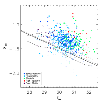
Figure 6.— Optical/UV-to-X-ray spectral slope ${\alpha}_{\rm ox}$ as a function of ${\ell}_{\rm uv}$; symbols are coded as in Figure 3. The solid/dotted line is the best-fit linear relation for RQQs from Just et al. (2007)/Steffen et al. (2006), while the dashed lines show the 25th and 75th percentiles for RQQs. Our sample shows the well-known tendency for RLQs to be X-ray bright relative to RQQs of comparable optical/UV luminosities.

Figure 7.— X-ray “excess” in RIQs and RLQs relative to comparable RQQs plotted as a function of radio loudness (top) and radio luminosity (bottom). The solid line corresponds to a linear multiplicative ratio of one and the dashed line to a ratio of three. The black crosses show median values within bins; the arms show the 25th–75th percentile range in each bin (values given in Table 5). Mean values are similar to medians and the error on the mean is much smaller than the interquartile range shown. Symbols are coded as in Figure 3.

Almost all of the ROSAT coverage is serendipitous; only 6/281 (2.1%) sources are found within $3^{\prime}$ of the aimpoint of the best ROSAT observation. The SDSS and FIRST surveys served as a source of targets for many XMM-Newton and Chandra observations; 34/202 (16.8%) sources are found within $2^{\prime}$ of the aimpoint of the best XMM-Newton observation, and 58/171 (33.9%) sources are found within $1^{\prime}$ of the aimpoint of the best Chandra observation. Some of these targeted objects also have serendipitous coverage and would be in our sample even absent the targeted observations: four of the objects targeted by XMM-Newton have off-axis Chandra coverage and two of the objects targeted by Chandra have off-axis ROSAT coverage. In total, then, 92/654 (14.1%) of the RIQs and RLQs in our primary sample were targeted for X-ray observations (of which 91/92 have X-ray detections). The analysis of luminosity correlations below was carried out including targeted objects to increase the size of the primary sample, but results are also provided for an “Off-axis” sample of sources with only serendipitous X-ray coverage and for the “Targeted” sample exclusively. Differences between the properties of the “Off-axis” and “Targeted” subsamples are discussed in $\S$5.4.2.

There may be cases in which the extraction region used to calculate the X-ray luminosity includes both nuclear and kpc-scale X-ray jet emission. Many X-ray jets have been discovered by Chandra (e.g., Sambruna et al. 2004; Marshall et al. 2005), and some would not be resolvable with ROSAT or even XMM-Newton. Additionally, in some instances the inner knot(s) of an X-ray jet might lie inside the Chandra extraction region. Generally even the inner knots of RLQs with X-ray jets are observed to be only a few percent as bright as the X-ray core (e.g., Marshall et al. 2005), which would not significantly change the calculated ${\ell}_{\rm x}$ values. The XJET catalog provides a useful listing of $\sim$100 objects with known extended X-ray jet or lobe emission. Out of the primary sample of 654 RIQs and RLQs, only 15 are listed in the XJET catalog. We examined X-ray images of all 15 objects and in no case did it appear likely that the extended X-ray emission could significantly increase the measured X-ray luminosity.

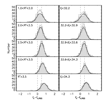
Figure 8.— Histograms of ${\ell}_{\rm x}-{\ell}_{\rm x,RQQ}$ (defined as in $\S$4) plotted in (increasing downward) bins of radio-loudness (left) and radio luminosity (right); the bins are identical to those in Table 5. The filled histograms contain X-ray-detected objects and the open histograms include upper limits. The vertical dashed lines correspond to linear multiplicative factors of 1 and 3 for the ratio of the X-ray luminosity of RIQs and RLQs to comparable RQQs. The solid/dotted curves are Gaussians fit to detected/all objects to investigate log-normality; there appears to be a tail of objects with high X-ray luminosities in the maximum radio-loudness and luminosity bins.

4. Comparison of the X-ray emission from RQQs, RIQs, and RLQs

Several previous studies have noted the tendency for RLQs to be more X-ray bright than RQQs of comparable optical/UV luminosity (e.g., Zamorani et al. 1981; see also discussion and references in $\S$1). We confirm that general result, and also quantify the degree to which RIQs and RLQs differ in X-ray brightness from RQQs as a function of radio loudness and luminosity. Our large and carefully constructed sample permits relatively fine-grained binning for such measurements.

The necessity of controlling for optical/UV luminosity when comparing RIQs and RLQs to RQQs is driven by the well-known steepening in RQQs of optical/UV-to-X-ray spectral slope with increasing optical/UV luminosity (e.g., ${\alpha}_{\rm ox}=-0.140\times{\ell}_{\rm uv}+2.705$ as given in Equation 3 of Just et al. 2007; other studies as listed in $\S$1.1 typically find similar results). As RLQs are X-ray brighter than RQQs at a given ${\ell}_{\rm uv}$, they have less negative values of ${\alpha}_{\rm ox}$. The median optical/UV-to-X-ray spectral slope for the full sample of RIQs and RLQs is ${\alpha}_{\rm ox}=-1.40$, and for RIQs/RLQs separately it is ${\alpha}_{\rm ox}=-1.50/-1.37$. The sample of RQQs we use for comparison (from Steffen et al. 2006) has a median ${\alpha}_{\rm ox}=-1.52$.

The ${\alpha}_{\rm ox}$ and ${\ell}_{\rm uv}$ values for the complete sample of RIQs and RLQs are plotted in Figure 6, along with the RQQ ${\alpha}_{\rm ox}({\ell}_{\rm uv})$ relations from Just et al. (2007) and Steffen et al. (2006), and the 25th and 75th percentiles for ${\alpha}_{\rm ox}$ for RQQs within each ${\ell}_{\rm uv}$ decade (from Table 5 of Steffen et al. 2006). The tendency of RQQs at lower luminosities to fall below the best-fit ${\alpha}_{\rm ox}({\ell}_{\rm uv})$ relation appears to be genuine (e.g., Steffen et al. 2006; Maoz et al. 2007); a larger sample is required to determine whether a qualitatively similar effect may apply to RIQs and RLQs. Like RQQs, RIQs and RLQs also show an anti-correlation between ${\alpha}_{\rm ox}$ and ${\ell}_{\rm uv}$ (a Spearman test gives $\rho=-0.31$, with a probability less than $p=5\times 10^{-5}$ that no correlation is present), albeit with a systematic offset toward less negative values of ${\alpha}_{\rm ox}$. Figure 6 also indicates that the degree to which RIQs and RLQs are brighter in X-rays than comparable RQQs is dependent upon radio loudness (the larger points, representing more radio-loud objects, are generally further above the RQQ ${\alpha}_{\rm ox}({\ell}_{\rm uv})$ relation); we now quantify this dependence.

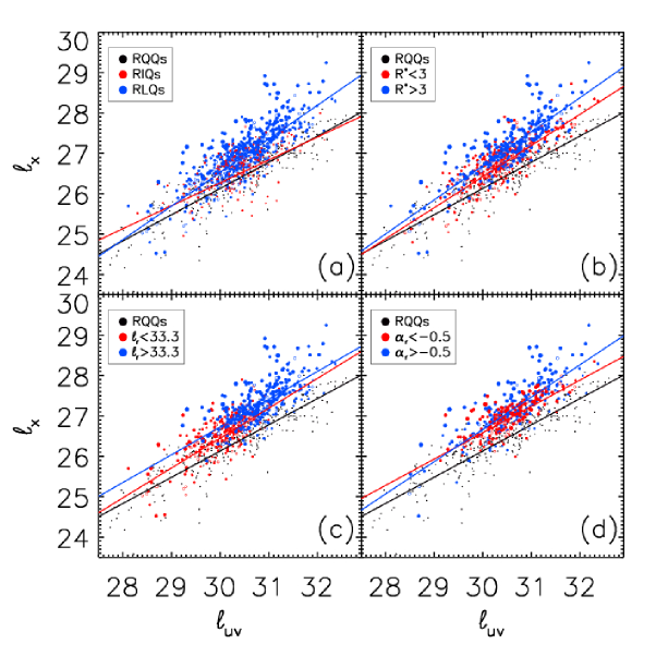
Figure 9.— X-ray luminosity as a function of optical/UV luminosity for RIQs and RLQs (a) and for various sub-samples of RLQs (b, c, d). The model considered is ${\ell}_{\rm x}=a_{\rm 0}+b_{\rm uv}{\times}{\ell}_{\rm uv}$ (where ${\ell}_{\rm x}$ and ${\ell}_{\rm uv}$ have been normalized prior to fitting as described in $\S$5). Filled symbols are X-ray detections and larger symbols are more radio-loud throughout. Solid lines show best-fit linear models.

The “excess” X-ray luminosity from RLQs may be defined as ${\ell}_{\rm x}-{\ell}_{\rm x,RQQ}$, where we take the expected X-ray luminosity for RQQs to be ${\ell}_{\rm x,RQQ}=0.709\times{\ell}_{\rm uv}+4.822$ (Equation 7 from Just et al. 2007) and use ${\ell}_{\rm uv}$ as measured for RIQs and RLQs. Figure 7 shows excess X-ray luminosity for the complete sample of RIQs and RLQs as a function of radio loudness and of radio luminosity, along with median values and the 25th–75th percentile range within bins of $R^{*}$ and ${\ell}_{\rm r}$. The median values and 25th and 75th percentiles plotted in Figure 7 are listed in Table 5. The mean values are consistent with the median values, and the error on the mean is much less than the 25th–75th percentile range. When expressed in linear units, the multiplicative factor by which the X-ray luminosity for RIQs and RLQs exceeds that of RQQs ranges (25th–75th percentiles) from 0.7–2.8 for RIQs through the canonical $\sim$3 for RLQs (e.g., Zamorani et al. 1981) to 3.4–10.7 for extremely radio-loud ($R^{*}>3.5$) RLQs, with a qualitatively similar increase in excess X-ray luminosity with increasing radio luminosity. Figure 8 shows the distribution of ${\ell}_{\rm x}-{\ell}_{\rm x,RQQ}$ (the shaded histogram is detected objects and the open histogram includes X-ray upper limits) within the same bins of $R^{*}$ (left) and ${\ell}_{\rm r}$ (right) as used to construct Table 5. The distribution of excess X-ray luminosity is reasonably well-characterized as log-normal (see overplotted Gaussians), with KS test probabilities $p>0.13$ in all cases. There appears to be a tail to brighter X-ray luminosity within the highest radio-loudness and luminosity bins (e.g., the percentage of objects above 1.645$\sigma$ from the mean is not 5% but rather 10%/11% within the most radio-loud/luminous bin, calculated using the fitted values for $\sigma$ and $\mu$). Similar results hold for the primary sample only (Table 6), with the mean values of ${\ell}_{\rm x}-{\ell}_{\rm x,RQQ}$ consistent between the full and primary samples across $R^{*}$ and ${\ell}_{\rm r}$ bins.

The excess X-ray luminosity may also be fit directly as a function of radio loudness or luminosity, for example as ${\ell}_{x}-{\ell}_{\rm x,RQQ}=a+b\times{R^{*}}$ or ${\ell}_{x}-{\ell}_{\rm x,RQQ}=a+b\times{\ell}_{\rm r}$, where $a$ and $b$ are fitting constants. We carry out such a fit using the IDL code of Kelly (2007), which utilizes Bayesian techniques that incorporate both uncertainties and upper limits. The best-fit models for the full sample are ${\ell}_{x}-{\ell}_{\rm x,RQQ}=(-0.354\pm 0.050)+(0.289\pm 0.018)\times{R^{*}}$ and ${\ell}_{x}-{\ell}_{\rm x,RQQ}=(0.450\pm 0.015)+(0.177\pm 0.014)\times({\ell}_{\rm r}-33.3)$. Excess X-ray luminosity is more strongly dependent upon radio-loudness than radio luminosity. Flat-spectrum RLQs may have excess X-ray luminosity more strongly correlated with radio properties than do steep-spectrum RLQs, with flat/steep spectrum RLQs having coefficients of $(0.352\pm 0.039)/(0.274\pm 0.040){\times}R^{*}$ and $(0.204\pm 0.027)/(0.088\pm 0.029)\times({\ell}_{\rm r}-33.3)$. The large amount of scatter in these relations prevents productive consideration of more complex models, but Figures 7 and 8 do suggest that these linear fits (to log quantities) may not adequately capture the apparent slow rise in X-ray excess at low radio-loudness or luminosity and the more rapid increase at higher $R^{*}$ or ${\ell}_{\rm r}$ values.

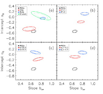
Figure 10.— Joint 90% (solid) and 68% (dotted) confidence ellipses for fitting X-ray luminosity as a (sole) function of optical/UV luminosity for various subsamples of RLQs. The model considered is ${\ell}_{\rm x}=a_{\rm 0}+b_{\rm uv}{\times}{\ell}_{\rm uv}$ (where ${\ell}_{\rm x}$ and ${\ell}_{\rm uv}$ have been normalized prior to fitting as described in $\S$5). RLQs with larger values of radio-loudness or luminosity or with flat radio spectra have greater best-fit intercepts than those with smaller values of radio-loudness or luminosity or with steep radio spectra.

5. Parameterizing the X-ray luminosity of RIQs and RLQs

We parameterize X-ray luminosity as a sole function of optical/UV luminosity and as a joint function of optical/UV and radio luminosity for various groupings of RIQs and RLQs, and also consider whether an additional dependence upon redshift is required. All fitting is carried out with the IDL code of Kelly (2007); using the Astronomy Survival Analysis (ASURV) package (e.g., Isobe & Feigelson 1990) gives similar results. The potential measurement errors in optical magnitudes and radio fluxes are generally small (see references to SDSS and FIRST in $\S$1), and most objects have sufficient X-ray counts that the uncertainties may be assumed to be dominated by intrinsic random flux variability (we use 20%/30%/40% or 0.0792/0.114/0.146 in log units for uncertainties on ${\ell}_{\rm r}/{\ell}_{\rm uv}/{\ell}_{\rm x}$, motivated by, e.g., $\S 3.5$ of Gibson et al. 2008). The luminosities are normalized prior to fitting as ${\ell}_{\rm r}-33.3,{\ell}_{\rm uv}-30.5,{\ell}_{\rm x}-27.0$ (the subtracted values are nearly the medians for the sample of RLQs). Results are given in Tables 7 and 8 and illustrated in Figures 9–17. For any given model fit the quoted parameter values are the median of draws from the posterior distribution and the errors are credible intervals corresponding to 1$\sigma$. See Appendix D for additional discussion of fitting methodology.

5.1. ${\ell}_{\rm x}({\ell}_{\rm uv})$

The first model we consider is X-ray luminosity as a sole function of optical/UV luminosity, such as is often applied to RQQs (e.g., Steffen et al. 2006; Just et al. 2007): ${\ell}_{\rm x}=a_{\rm 0}+b_{\rm uv}\times{\ell}_{\rm uv}$. It is most convenient to treat ${\ell}_{\rm x}$ as the dependent variable for the purposes of fitting, given the X-ray limits (and perhaps also most appropriate for our predominantly optically-selected sample of RIQs and RLQs, whose X-ray properties were not considered in selection). Since our analysis is comparative in nature, it suffices to maintain consistency and so we do not also calculate coefficients treating ${\ell}_{\rm uv}$ as the dependent variable, nor do we calculate a bisector fit. This approach also simplifies analysis when additional variables are considered. We first re-fit the RQQs from Steffen et al. (2006) using the same procedure we adopt for analyzing the RIQs and RLQs, to demonstrate the consistency of this method with previous work. Our results agree with those of Steffen et al. (2006) for their Equation 1a (see also Appendix D). We also re-fit the luminous Einstein RLQs from Worrall et al. (1987) separately, to assess the influence this subsample exerts upon the full sample. Finally, we fit the full sample and then also fit various groupings of RIQs and RLQs. Results for this model are given on the left side of Table 7 and plotted in Figure 9.

The general tendencies revealed by Figure 9 are (9a) RIQs have X-ray luminosities only modestly greater than those of RQQs of comparable optical/UV luminosities, whereas RLQs become increasingly X-ray bright relative to comparable RQQs as ${\ell}_{\rm uv}$ increases; (9b) when RLQs are subdivided by radio loudness, RLQs with $R^{*}>3$ are more X-ray luminous than those with $R^{*}<3$; (9c) when RLQs are subdivided by radio luminosity, RLQs with ${\ell}_{\rm r}>33.3$ are more X-ray luminous than those with ${\ell}_{\rm r}<33.3$; (9d) RLQs with flat radio spectra are more X-ray luminous than those with steep radio spectra, and in particular almost all of the most X-ray luminous RLQs (with ${\ell}_{\rm x}>28$) have flat radio spectra. There does not appear to be any grouping of RIQs or RLQs that contains objects with X-ray luminosities less than those of comparable RQQs at any optical/UV luminosities; this is broadly consistent with RIQs and RLQs being similar to RQQs but with an “extra” source of X-ray emission whose strength depends upon radio properties. Over all groupings and models, there is a general tendency for the RLQs at the highest optical/UV luminosities to lie above their best-fit models (to a degree exceeding any possible slight systematic flattening of the slope due to the fitting method; see Appendix D), and this structure in the residuals suggests that a linear fit (to logarithmic quantities) of X-ray luminosity as a sole function of optical/UV luminosity is not an adequate model even when applied within subgroups of RLQs, at least for particularly radio-loud, luminous, or flat-spectrum RLQs.

Joint 68% and 90% confidence ellipses for the various fits to this model are plotted in Figure 10. In all panels the RQQ result is plotted as a black ellipse for comparison. It can be seen in (10a) that the confidence region for RIQs is near to that of RQQs; the modest radio loudness and radio luminosity of RIQs generally do not appear to enhance substantially their X-ray emission. In contrast, the confidence region for RLQs is well separated from that of RQQs, with both a greater model intercept and slope. It can also be seen that our sample substantially increases the precision with which the model parameters can be assessed over that provided by previous studies, such as that of Worrall et al. (1987) for their Einstein sample of RLQs (recall we use 93 of their 114 objects). In (10b), (10c), and (10d) the confidence regions for RLQs with $R^{*}>3$, ${\ell}_{\rm r}>33.3$, and ${\alpha}_{\rm r}>-0.5$ are offset from their weaker RLQ counterparts, which are themselves still fully distinct from RQQs. The increased X-ray brightness for RLQs with $R^{*}>3$ or ${\ell}_{\rm r}>33.3$ is primarily due to a larger intercept in the modeled relation. It is possible that flatter radio spectra objects may have a stronger dependence of ${\ell}_{\rm x}$ on ${\ell}_{\rm uv}$, although the 90% confidence regions overlap in projection onto the slope variable. The trends displayed in (10b) and (10d) are qualitatively similar to those shown by Worrall et al. (1987) in their Figure 1.

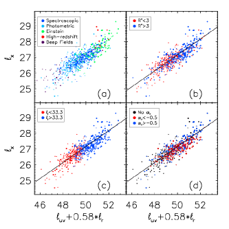
Figure 11.— X-ray luminosity as a joint function of optical/UV and radio luminosity for various sub-samples of RLQs. The model considered is ${\ell}_{\rm x}=a_{\rm 0}+b_{\rm uv}{\times}{\ell}_{\rm uv}+c_{\rm r}{\times}{\ell}_{\rm r}$ (where ${\ell}_{\rm x}$, ${\ell}_{\rm uv}$, and ${\ell}_{\rm r}$ have been normalized prior to fitting as described in $\S$5). Filled symbols are X-ray detections and larger symbols are more radio-loud throughout. The x-axis is based on the best-fit model for RLQs, for which $c_{\rm r}\simeq 0.58{\times}b_{\rm uv}$. The black solid line in panels (b), (c), and (d) is the best-fit model for RLQs.

5.2. ${\ell}_{\rm x}({\ell}_{\rm uv},{\ell}_{\rm r})$

5.2.1 Inclusion of radio luminosity as a fit parameter

The second parameterization we consider is X-ray luminosity as a joint function of optical/UV luminosity and radio luminosity: ${\ell}_{\rm x}=a_{\rm 0}+b_{\rm uv}\times{\ell}_{\rm uv}+c_{\rm r}\times{\ell}_{\rm r}$. The resulting coefficients obtained from fitting various groupings of RIQs and RLQs are listed on the right side of Table 7. The optical/UV luminosity coefficient is now $b_{\rm uv}=0.506$ for RLQs and $b_{\rm uv}=0.432/0.439/0.471$ for highly radio-loud/radio-luminous/flat-spectrum RLQs, compared to the $b_{\rm uv}=0.649$ for RQQs; this suggests that the apparently stronger dependence of RLQ X-ray luminosity upon ${\ell}_{\rm uv}$ indicated in the previous model of ${\ell}_{\rm x}({\ell}_{\rm uv})$ was actually reflecting the influence of radio luminosity, which is now explicitly considered. The best-fit model for RIQs indicates that radio properties do not strongly infuence the X-ray luminosity of RIQs ($c_{\rm r}$ is formally consistent with zero). Figure 11 plots ${\ell}_{\rm x}$ versus ${\ell}_{\rm uv}+0.58\times{\ell}_{\rm r}$. This choice of variables is motivated by the coefficients of the ${\ell}_{\rm x}({\ell}_{\rm uv},{\ell}_{\rm r})$ model for RLQs, for which $c_{\rm r}$ is $\simeq 0.58{\times}b_{\rm uv}$ (Table 7). Collapsing the ${\ell}_{\rm uv}-{\ell}_{\rm r}$ plane to a single joint variable simplifies presentation of the modeling results and enables ready comparison of the properties of subgroups of RLQs to those of RLQs as a whole. It can be seen from (11a) that the Einstein sample of RLQs dominates the highest luminosity region of the full sample, which also contains the high-redshift sample objects. Conversely, the lowest luminosity region of the full sample is strongly influenced by the deep-field sample objects, although there are many primary sample photometric quasars in this region as well. In (11b), (11c), and (11d), data for the same subgroups of RLQs as in Figure 9 are shown along with the best-fit ${\ell}_{\rm x}({\ell}_{\rm uv},{\ell}_{\rm r})$ model for RLQs for comparison. The subgroups of RLQs do not deviate strongly from the trend for RLQs in general in these coordinates, although the particularly radio and optical/UV luminous RLQs from the Einstein sample (along with a few high-redshift objects) are still excessively X-ray bright.

Figure 12.— Joint 90% confidence ellipses for fitting X-ray luminosity as a function of radio and optical/UV luminosity. The model considered is ${\ell}_{\rm x}=a_{\rm 0}+b_{\rm uv}{\times}{\ell}_{\rm uv}+c_{\rm r}{\times}{\ell}_{\rm r}$ (where ${\ell}_{\rm x}$, ${\ell}_{\rm uv}$, and ${\ell}_{\rm r}$ have been normalized prior to fitting as described in $\S$5). The legend in (b) also applies to (a) and the legend in (d) also applies to (c). See $\S$5.2 for discussion.

Joint 90% confidence ellipses (calculated after collapsing the third dimension for ease of viewing) for the various fits to this model are plotted in Figure 12. The full, primary, and Einstein samples are plotted in (12a) and (12b), as are the subgroups of RLQs with $R^{*}<3$ and $R^{*}>3$. The parameters for the primary sample of SDSS RIQs and RLQs are consistent with those of the full sample (not unexpected, since the primary sample makes up a majority of the full sample). There is no evidence of a statistically significant difference in the X-ray luminosity dependence of these subgroups upon optical/UV luminosity. There is suggestive support for Einstein RLQs and (relatedly) for RLQs with $R^{*}>3$ possessing a stronger dependence of X-ray luminosity upon radio luminosity, but the projected confidence ellipses all overlap in (12b). The joint 90% confidence ellipses for the ${\ell}_{\rm x}({\ell}_{\rm uv},{\ell}_{\rm r})$ model applied to subgroups of RLQs divided by radio luminosity and by radio spectral index are plotted in (12c) and (12d), along with the result for RLQs in general provided for comparison. Flat-spectrum RLQs are X-ray brighter than steep-spectrum RLQs due to a larger intercept, but have a consistent dependence of X-ray luminosity upon both optical/UV and radio luminosity. In possible contrast, RLQs with ${\ell}_{\rm r}<33.3$ and those with ${\ell}_{\rm r}>33.3$ share similar best-fit intercepts, but the more radio-luminous RLQs may have a greater/lesser dependence of ${\ell}_{\rm x}$ upon ${\ell}_{\rm r}/{\ell}_{\rm uv}$, although the confidence ellipses overlap in projection onto $c_{\rm r}/b_{\rm uv}$.

5.2.2 A “radio-adjusted” ${\ell}_{\rm x}({\ell}_{\rm uv})$ relation for RIQs and RLQs

We consider briefly whether RIQs and RLQs can be treated as similar to RQQs but with an additional jet-linked contribution to the X-ray luminosity (which could imply a consistent disk/coronal structure). If so, then after accounting for the influence of radio emission, the X-ray luminosity in RIQs and RLQs should be correlated with optical/UV luminosity through a relation similar to that for RQQs. RIQs display no significant dependence of X-ray luminosity upon radio luminosity and may share the same dependence upon optical/UV luminosity as holds for RQQs, although this is not strongly constrained in our data.

One method of investigating a “radio-adjusted” ${\ell}_{\rm x}({\ell}_{\rm uv})$ relation could be to set the radio luminosity in the best-fit RLQ ${\ell}_{\rm x}({\ell}_{\rm uv},{\ell}_{\rm r})$ model to a value representative of RQQs. This requires an accurate parameterization of ${\ell}_{\rm r}({\ell}_{\rm uv})$ for RQQs, a difficult function to evaluate given the inherent radio weakness of RQQs. A simple model could have radio luminosity proportional to optical/UV luminosity as ${\ell}_{\rm r}=\alpha+\beta\times{\ell}_{\rm uv}$; in this case ${\ell}_{\rm x}({\ell}_{\rm uv},{\ell}_{\rm r})$ would transform to ${\ell}_{\rm x}({\ell}_{\rm uv})$ as (adding in the implicit luminosity normalizations) ${\ell}_{\rm x}-27=a_{\rm 0}+c_{\rm r}\times(\alpha+30.5\beta-33.3)+(b_{\rm uv}+c_{\rm r}\beta)\times({\ell}_{\rm uv}-30.5)$. White et al. (2007) present a correlation (their Equation 2) that extends to low radio-loudness values ($R^{*}<1$) and is equivalent to $\alpha=4.57$ and $\beta=0.85$. Adopting these values of $\alpha$ and $\beta$, the RLQ fit of ${\ell}_{\rm x}=-0.100+0.506{\ell}_{\rm uv}+0.292{\ell}_{\rm r}$ becomes ${\ell}_{\rm x}=-0.919+0.754{\ell}_{\rm uv}$; this may be compared with the best-fit RQQ relation of ${\ell}_{\rm x}=-0.545+0.649{\ell}_{\rm uv}$ (all fitted coefficients from Table 7). The slope for RLQs in the radio-adjusted relation is closer to but slightly larger than that for RQQs (the difference is $0.105\pm 0.049$). Since we have not yet taken the likely beaming of some fraction of the X-ray emission in RLQs into account, this result does not mandate that the disk/corona in RLQs is more X-ray efficient at high optical/UV luminosities than in RQQs. (We demonstrate in $\S$6 that the RLQ ${\ell}_{\rm x}({\ell}_{\rm uv},{\ell}_{\rm r})$ fit can be reproduced assuming a disk/coronal scaling as in RQQs plus a jet component.) The difference in intercepts as compared to the RQQ relation may be reflective of greater beaming of radio emission in the RLQs (although some RQQs may have a boosted component of radio emission; e.g., Miller et al. 1993; Falcke et al. 1996), in which case the RQQ relation ought to have the radio luminosity similarly enhanced prior to substitution for a first-order comparison. For illustrative purposes, accounting for an additional beaming enhancement of a factor of 19 (e.g., corresponding to an inclination of $\simeq 12^{\circ}$ with $\gamma=10.5$; see $\S$6) would change the transformed RLQ intercept to match the RQQ result.

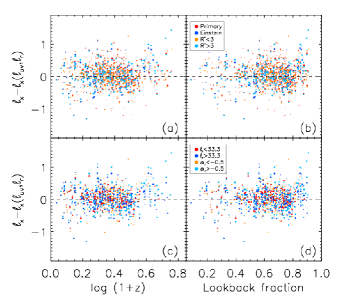
Figure 13.— Residuals for best-fit results for X-ray luminosity parameterized by optical/UV and radio luminosity, plotted against redshift and fractional lookback time. The legend in (b) also applies to (a) and the legend in (d) also applies to (c). A single object may be a member of two categories in a given panel, in which case the residual values from the separate fits to each category are each plotted at the redshift of that object. There is no apparent redshift dependence. See $\S$5.3 for discussion.

5.3. ${\ell}_{\rm x}({\ell}_{\rm uv},{\ell}_{\rm r},z)$

5.3.1 Inclusion of redshift as a fit parameter

We now investigate whether there is a dependency upon redshift in addition to the dependencies upon optical/UV and radio luminosity. Although the ${\ell}_{\rm x}({\ell}_{\rm uv},{\ell}_{\rm r})$ residuals (see Figure 13) do not show any obvious redshift dependence, it is in principle possible that some of the apparent luminosity dependence might actually be driven by redshift evolution. We test this possibility by including the redshift dependence as a parameter when modeling, by fitting ${\ell}_{\rm x}({\ell}_{\rm uv},{\ell}_{\rm r},z)$, where again the luminosities are normalized prior to fitting. The redshift dependence is put in terms of $\log(1+z)$ or lookback fraction [${\tau}_{\rm z}$ = 1$-$age($z$)/age($z=0$)]. The best-fit model for the full sample is ${\ell}_{\rm x}=(-0.098\pm 0.051)+(0.482\pm 0.036)\times{\ell}_{\rm uv}+(0.273\pm 0.019)\times{\ell}_{\rm r}+(0.000\pm 0.128)\times{\log}(1+z)$; when RLQs only are considered, the best-fit model is ${\ell}_{\rm x}=(-0.109\pm 0.052)+(0.503\pm 0.042)\times{\ell}_{\rm uv}+(0.293\pm 0.027)\times{\ell}_{\rm r}+(0.025\pm 0.131)\times{\log}(1+z)$. When the redshift dependence is expressed instead in terms of the fractional lookback time ${\tau}_{\rm z}$, the best-fit model for the full sample is ${\ell}_{\rm x}=(-0.064\pm 0.072)+(0.488\pm 0.034)\times{\ell}_{\rm uv}+(0.273\pm 0.019)\times{\ell}_{\rm r}+(-0.052\pm 0.109)\times{\tau}_{\rm z}$; when RLQs only are considered, the best-fit model is ${\ell}_{\rm x}=(-0.065\pm 0.074)+(0.511\pm 0.042)\times{\ell}_{\rm uv}+(0.292\pm 0.027)\times{\ell}_{\rm r}+(-0.053\pm 0.111)\times{\tau}_{\rm z}$. In all these cases the difference between the coefficient for the redshift term and zero is not statistically significant, and the joint 68% and 90% confidence ellipses with the optical/UV and radio luminosity coefficients include zero (Figure 14). The redshift coefficients for the ${\log}(1+z)/{\tau}_{\rm z}$ models when fitting the primary sample, spectroscopic sample, or Einstein sample alone are $-0.500\pm 0.167$/$-0.364\pm 0.140$, $-0.351\pm 0.245$/$-0.337\pm 0.202$, or $0.775\pm 0.443/0.282\pm 0.379$, respectively. The indicated redshift dependence is marginal (3.0/2.6, 1.4/1.7, or 1.7/0.7$\sigma$), and the direction of the potential trend is inconsistent between the primary and Einstein samples; recall also that Worrall et al. (1987), using independent methods, found no significant redshift dependence among the Einstein objects. The superior coverage of the ${\ell}-z$ plane provided by the full and RLQ samples leads us to favor those results.

Figure 14.— Consideration of redshift dependence. The first model investigated is ${\ell}_{\rm x}=a_{\rm 0}+b_{\rm uv}{\times}{\ell}_{\rm uv}+c_{\rm r}{\times}{\ell}_{\rm r}+d_{\rm z}{\times}{\log}(1+z)$ (where ${\ell}_{\rm x}$, ${\ell}_{\rm uv}$, and ${\ell}_{\rm r}$ have been normalized prior to fitting as described in $\S$5); the second model investigated replaces ${\log}(1+z)$ with the fractional lookback time ${\tau}_{\rm z}$. Joint 90% (solid) and 68% (dotted) confidence ellipses are plotted for the full sample (red) and for the sample of RLQs (blue). The difference between the coefficients for redshift dependence and zero is not statistically significant.

We find no evidence for a dependence upon redshift for the X-ray emission properties of the full sample or RLQs alone. The degree to which otherwise comparable RIQs or RLQs at different redshifts could differ in X-ray luminosity may be constrained via the value and 1$\sigma$ errors on the best-fit coefficient to the redshift term. For the full sample, the coefficient of $(0.000\pm 0.128)\times{\log}(1+z)$ suggests a maximum evolution (1$\sigma$, i.e., using 0.000+0.128 for the coefficient) in X-ray luminosity between redshift $z=0$ and $z=5$ of ${\ell}_{\rm x,z=0}-{\ell}_{\rm x,z=5}=0.100$, or a ratio in linear units of 1.26. This suggests that the X-ray luminosity of otherwise comparable RIQs or RLQs has not changed by more than 30% over $z=0-5$. For RLQs only, a similar analysis suggests a maximum change of $\lower 2.0pt\hbox{$\,\buildrel\scriptstyle<\over{\scriptstyle\sim}\,$}35$%. The ${\tau}_{\rm z}$ best-fit coefficients similarly suggest a maximum redshift-driven change in X-ray luminosity for the full sample or for RLQs of $\lower 2.0pt\hbox{$\,\buildrel\scriptstyle<\over{\scriptstyle\sim}\,$}30$% over $z=0-5$. Although the fraction of quasars that are RLQs is dependent upon redshift (e.g., Jiang et al. 2007), the X-ray properties of individual RIQs and RLQs do not appear to differ strongly when comparing objects at low versus high redshift. Apparently the cosmic evolution in the efficiency of generating RLQs does not substantially impact RLQ structure post-formation.

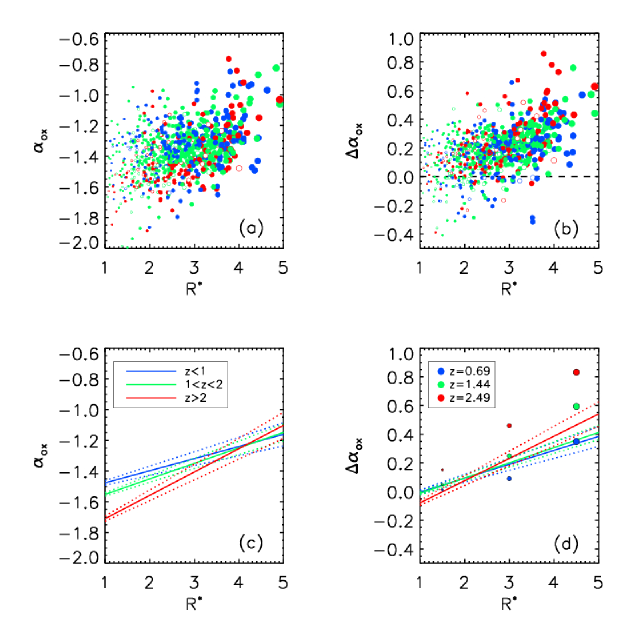
Figure 15.— Consideration of relative X-ray brightness as a function of radio-loudness. The full sample of RIQs and RLQs is shown in (a) for ${\alpha}_{\rm ox}(R^{*})$ and in (b) for ${\Delta}{\alpha}_{\rm ox}(R^{*})$, with blue, green, and red colors indicating low, medium, or high redshift ($z<1$, $1<z<2$, and $z>2$, respectively). Best-fit trend lines are shown in (c) and (d) with the 1$\sigma$ errors on the slopes indicated by dashed lines. The expected enhancement in X-ray brightness from the $(1+z)^{4}$ dependence of IC/CMB jet-linked X-ray emission is also plotted in (d) for comparison; the set of points at $R^{*}$=1.5, 3, and 4.5 correspond to models in which the jet-linked fraction of the X-ray continuum (prior to considering redshift) is 1%, 10%, and 99%, respectively.

5.3.2 Dependence of relative X-ray brightness on redshift

An alternative manner of visualizing the potential redshift dependence of the X-ray luminosity of RIQs and RLQs and of searching for redshift evolution as a function of radio-loudness is to construct a multiwavelength color-color plot and group objects within separate redshift bins. Figure 15a shows ${\alpha}_{\rm ox}$ plotted versus $R^{*}$ for the full sample divided into low, medium, and high redshift ($z<1$, $1<z<2$, and $z>2$, respectively). Objects become increasingly X-ray bright (with less negative values of ${\alpha}_{\rm ox}$) as they become increasing radio-loud, as previously shown in Figure 7, but there is no obvious difference in this trend with redshift. Fitting ${\alpha}_{\rm ox}(R^{*})$ does suggest that the slope steepens slightly with redshift, but this is offset by a decreased intercept (Figure 15c; see also Figure 5 of Lopez et al. 2006). It is preferable to take the dependence of X-ray luminosity upon optical/UV luminosity into account when constructing the optical/UV-to-X-ray color. We calculate ${\Delta}{\alpha}_{\rm ox}={\alpha}_{\rm ox}-{\alpha}_{\rm ox}({\ell}_{\rm uv})$ by taking ${\alpha}_{\rm ox}({\ell}_{\rm uv})$ from the Just et al. (2007) relation for RQQs (their Equation 3). Figure 15b shows ${\Delta}{\alpha}_{\rm ox}$ plotted versus $R^{*}$ for the full sample grouped into low, medium, and high redshift bins. There is no obvious stratification by redshift, but here fitting ${\Delta}{\alpha}_{\rm ox}(R^{*})$ suggests that the slight increase in slope with increasing redshift may result in a slight increase in relative X-ray brightness, at least for RLQs with $R^{*}>2$ (Figure 15d). It is possible that a disproportionate number of objects in the high-redshift bin with low line-of-sight inclinations could produce this result. The best-fit model parameters are given in Table 8. Two-dimensional KS tests indicate that the distribution of ${\alpha}_{\rm ox}-R^{*}$ is inconsistent between different redshift bins (low-mid, mid-high, or low-high), but that of ${\Delta}{\alpha}_{\rm ox}-R^{*}$ is not ($p\lower 2.0pt\hbox{$\,\buildrel\scriptstyle>\over{\scriptstyle\sim}\,$}0.12$ for all cases).

It has been suggested that X-ray jets for which inverse Compton scattering of cosmic microwave background photons (IC/CMB; e.g., Tavecchio et al. 2000) provides the primary emission component should become the dominant source of RLQ X-ray emission at high redshift (e.g., Rees & Setti 1968; Schwarz 2002). We estimate the enhancement in total X-ray luminosity from this process for sources at redshifts of 0.69/1.44/2.48 (the medians within the low/medium/high groupings) and for a jet-linked fraction $j$ of the nuclear X-ray emission (prior to accounting for the redshift dependence of IC/CMB X-ray emission) of 1%, 10%, and 99%. This is expressed in terms of an increase in ${\Delta}{\alpha}_{\rm ox}$ as $0.384\times\log{[j(1+z)^{4}+(1-j)]}$, where the coefficient converts the increase in ${\ell}_{\rm x}$ to a flattening of the optical/UV-to-X-ray spectral slope. The results are plotted (in increasing order of jet dominance) at radio-loudness values of 1.5, 3, and 4.5 in Figure 14d. It can be seen that the $(1+z)^{4}$ dependence of X-ray jet-linked IC/CMB emission would lead for these parameters to a stronger splitting with redshift than is observed. We find that the X-ray luminosities within our sample of RIQs and RLQs are unlikely to include significant contributions from X-ray IC/CMB jet emission. In principle it is possible that extremely bright X-ray jet features could be routinely found outside of the extraction regions we use to measure the X-ray luminosity, but to our knowledge such sources are extremely rare. This is consistent with the general lack of observed high-redshift RLQs in which the X-ray jet outshines the core (e.g., Bassett et al. 2004; Lopez et al. 2006).

5.4. Additional considerations

We briefly examine four additional topics relevant to the analysis of luminosity correlations: the impact of the selection method, the influence of targeted sources, the normality of the variables, and the potential for spurious or inaccurate results due to luminosity dispersion effects.

5.4.1 Optical versus radio selection

As discussed in $\S$2.1.1, the median properties of a quasi-radio-selected sample of RIQs and RLQs (constructed from SDSS spectroscopic quasars by requiring the “FIRST” target flag to be set) are similar to those of “QSO/HIZ” targeted SDSS spectroscopic quasars (with substantial overlap between these samples). The dependence of X-ray luminosity upon optical/UV and radio luminosities is also similar for the “FIRST” and for the “QSO/HIZ” samples, as may be seen from the best-fit relations given in Table 7. Joint 68% and 90% confidence contours from fitting the “FIRST” and the “QSO/HIZ” samples to ${\ell}_{\rm x}=a_{\rm 0}+b_{\rm uv}\times{\ell}_{\rm uv}+c_{\rm r}\times{\ell}_{\rm r}$ are provided in Figure 16, where it can be seen that the parameter values are consistent. By excluding the small fraction of objects with ${\Delta}(g-i)>1$ we omit strongly dust-reddened RLQs, which may be associated with young quasars (e.g., Urrutia et al. 2008, 2009). Within the relative color range we accept, there does not appear to be a difference in the X-ray properties of SDSS RIQs and RLQs selected by color compared to those selected due to radio emission. Presumably the X-ray emission mechanisms are likewise similar, and so the results from $\S$5 and the modeling in $\S$6 are generally applicable.

5.4.2 Influence of targeted objects

Only 14.1% of RIQs and RLQs within the primary sample were targeted for X-ray observations ($\S$3.4), with the remainder possessing serendipitous off-axis coverage. Inclusion of the targeted sources does not bias the results of the luminosity correlation analysis, although there are some minor differences in the properties of targeted and off-axis objects. Compared to those objects observed serendipitously, the targeted RIQs and RLQs are at somewhat lower redshifts (median $z$ of 1.05 versus 1.45) but are also brighter (median $m_{\rm i}$ of 17.94 versus 19.54) and so have modestly higher optical/UV luminosities (median ${\ell}_{\rm uv}$ of 30.74 versus 30.33). The targeted RIQs and RLQs are also somewhat more radio-loud (median $R^{*}$ of 3.09 versus 2.44) and $\sim$40% X-ray brighter relative to optical/UV luminosity (median ${\ell}_{\rm x}-{\ell}_{\rm x,RQQ}$ of 0.53 versus 0.38, with ${\ell}_{\rm x}-{\ell}_{\rm x,RQQ}$ as defined in $\S$4). Presumably, targets were preferentially selected from sources already known to be X-ray bright.

The results of parameterizing X-ray luminosity for the off-axis objects are similar to those obtained for the full and primary samples (Table 7). The differences between the best-fit parameters for the slopes for the off-axis sample compared to the full or primary samples are essentially zero. Fitting the targeted objects separately indicates they possess a weaker dependence of X-ray luminosity upon optical/UV luminosity and perhaps a stronger dependence upon radio luminosity than do the full or primary samples, although their parameters are consistent with those of the spectroscopic sample.

Figure 16.— Comparison of a quasi-radio-selected (red ellipses) sample of RIQs and RLQs to an optically-selected (blue ellipses) sample (both drawn from SDSS/FIRST data; there is $\,\buildrel\scriptstyle>\over{\scriptstyle\sim}\,$90% overlap), illustrated with joint 90% (solid) and 68% (dotted) confidence ellipses for the model ${\ell}_{\rm x}=a_{\rm 0}+b_{\rm uv}{\times}{\ell}_{\rm uv}+c_{\rm r}{\times}{\ell}_{\rm r}$. The axes are scaled to match Figure 12. The RIQs and RLQs targeted by SDSS as FIRST sources have properties consistent with those targeted due to optical colors.

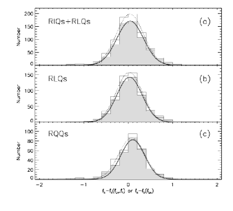
Figure 17.— Evaluation of normality for residuals from fitting X-ray luminosity as a joint function of optical/UV and radio luminosity (RIQs and RLQs, top panel; RLQs, middle panel; fits from Table 7) and as a sole function of optical/UV luminosity (RQQs, bottom panel; data from Steffen et al. 2006). The open histograms include limits and are fit with Gaussians as indicated by the dotted curves, while the filled histograms are detections only and are fit with Gaussians as indicated by the solid curves.

5.4.3 Log-normality of residuals

A presumption that considered variables are normally distributed is inherent in the chosen method of analysis (and indeed in most parametric modeling), and can be checked by examining the residuals from the best-fit models for X-ray luminosity in our sample of RIQs and RLQs. Histograms of the residual X-ray luminosity for RIQs and RLQs, RLQs alone, and RQQs are provided in Figure 17. While it is not clear a priori that the RIQs and RLQs considered here ought to show normally-distributed residual X-ray luminosity (in logarithmic units), since there are distinct X-ray emission mechanisms for RIQs and RLQs (disk/corona and jet-linked) as opposed to a single dominant X-ray emission mechanism (disk/corona) in RQQs, it may be seen in Figure 17 that the distributions closely match the overplotted best-fit Gaussians. Unfortunately the presence of limits in our sample makes it difficult to utilize standard tests for normality. We examine the distribution of detected objects and also the distribution of all objects, treating limits as detections for this calculation only. The distribution of residual X-ray luminosity is acceptably characterized as normal, with KS test probabilities $p>0.18$ in all cases. While this is best regarded as suggestive rather than conclusive, it does indicate that our methodology is unlikely to produce biased results due to substantial underlying non-normality.

There appears to be a tail of X-ray weak objects within the RQQ sample (17c), some of which might be low-redshift BAL RQQs. The sample of RIQs and RLQs (17a) also appears to show an X-ray weak tail, perhaps less prominently for RLQs only (17b). These may again be BAL objects, which decrease in percentage as radio-loudness increases (e.g., Shankar et al. 2008). However, in contrast to the situation for RQQs, there may also be an X-ray bright tail for RIQs and RLQs (for example, the percentage of objects above 1.645$\sigma$ from the mean is not 5% but rather 8%/8% for (RIQs+RLQs)/RLQs, calculated using the fitted values for $\sigma$ and $\mu$; it is 6% for RQQs). These X-ray bright objects are generally members of the set of particularly radio-loud or radio-luminous RLQs, and hence may be jet-dominated at X-ray frequencies.

5.4.4 Robustness of luminosity correlations

The degree of inherent scatter in the luminosities can affect the results of correlation studies. For example, Yuan et al. (1998) demonstrated that when the optical/UV luminosity scatter ${\sigma}_{\rm uv}$ is significantly larger than the X-ray luminosity scatter ${\sigma}_{\rm x}$, a fit to ${\alpha}_{\rm ox}({\ell}_{\rm uv})$ over a limited range of ${\ell}_{\rm uv}$ can indicate an anti-correlation where none necessarily exists. Relatedly, ${\sigma}_{\rm uv}\gg{\sigma}_{\rm x}$ can give a fitted slope for the ${\ell}_{\rm x}({\ell}_{\rm uv})$ relation less than unity even if these luminosities are actually proportional (when the considered luminosity ranges are small). In general, examined luminosity correlations are significantly less likely to yield spurious or inaccurate results with a sample spanning a large range in luminosities relative to the observed dispersion (e.g., see discussion in $\S$5 of Just et al. 2007), as does our sample.

It is possible to assess the luminosity scatter through consideration of the standard deviation of the residuals about the ${\ell}_{\rm x}({\ell}_{\rm uv},{\ell}_{\rm r})$ relation. For the primary sample, these values are 0.34/0.71/1.30 for ${\ell}_{\rm x}/{\ell}_{\rm uv}/{\ell}_{\rm r}$, with corresponding 5th–95th percentile luminosity ranges of 25.81–27.62/29.40–31.26/31.47–34.46 (treating X-ray limits as detections for this calculation only). This fit is performed treating ${\ell}_{\rm x}$ as the dependent variable, so the residuals about this fit are larger than the inherent scatter. We use a Monte Carlo approach to determine the corresponding ${\sigma}_{\rm x}/{\sigma}_{\rm uv}/{\sigma}_{\rm r}$ values. For simplicity, we simulate ${\ell}_{\rm uv,mod}$ as uniformly distributed ($n=654$) between 29.50 and 31.25, with ${\ell}_{\rm r,mod}$ = ${\ell}_{\rm uv,mod}$ + 2.5 (with random log-normal scatter of ${\sigma}_{\rm R^{*}}$) and ${\ell}_{\rm x,mod}$ calculated from ${\ell}_{\rm x}({\ell}_{\rm uv},{\ell}_{\rm r})$. Then random log-normal scatter ${\sigma}_{\rm x}/{\sigma}_{\rm uv}/{\sigma}_{\rm r}$ is added to the model luminosities and the standard deviations of the residuals and the luminosity ranges are calculated. A good match to the observed data is provided with ${\sigma}_{\rm x}/{\sigma}_{\rm uv}/{\sigma}_{\rm r}$ = 0.28/0.32/0.42, and ${\sigma}_{\rm R^{*}}=0.55$ gives a radio-loudness standard deviation of $\simeq$0.75 in agreement with the primary sample.

We assess the impact of such inherent scatter by fitting the simulated data (including X-ray censoring as described in $\S$6.1.3). This scatter acts to depress the dependence of X-ray luminosity upon optical/UV and radio luminosities, so that fitted values of $b_{\rm uv}$ and $c_{\rm r}$ are slightly lower than those used in the input ${\ell}_{\rm x}({\ell}_{\rm uv},{\ell}_{\rm r})$ relation. The observed best-fit values of $b_{\rm uv}\simeq 0.48$ and $c_{\rm r}\simeq 0.26$ for the primary sample would result in fitted coefficients of 0.39 and 0.23, respectively, and may themselves be obtained for input coefficients of $\simeq$0.6 and $\simeq$0.3, respectively. Further, data simulated with an input model of ${\ell}_{\rm x}({\ell}_{\rm uv},{\ell}_{\rm r})$ that is then fit as ${\ell}_{\rm x}({\ell}_{\rm uv})$ produce fitted values for $b_{\rm uv}$ greater than the input coefficient (e.g., fitted $b_{\rm uv}=0.67\pm 0.03$ for input $b_{\rm uv}/c_{\rm r}$=0.6/0.3), as suggested in $\S$5.2.1.

A contribution to the X-ray luminosity linked to the radio luminosity appears to be mandated for RIQs and RLQs. For the derived inherent scatter, it is not possible to reproduce the observed best-fit ${\ell}_{\rm x}({\ell}_{\rm uv},{\ell}_{\rm r})$ relation for the primary sample with an input model using ${\ell}_{\rm x}({\ell}_{\rm uv})$ as for RQQs. With the luminosity ranges of our primary sample, the $b_{\rm uv}\simeq 0.65$ observed for RQQs may result from an input coefficient of $\simeq$0.85 (1.0 is excluded; see, e.g., $\S$3.5 of Strateva et al. 2005). Data simulated with an input model of ${\ell}_{\rm x}\propto 0.85\times{\ell}_{\rm uv}$ that is then fit as ${\ell}_{\rm x}({\ell}_{\rm uv},{\ell}_{\rm r})$ produce fitted coefficients of $b_{\rm uv}=0.56\pm 0.03$ and $c_{\rm r}=0.09\pm 0.02$. If ${\ell}_{\rm r}$ is initially taken directly from ${\ell}_{\rm uv}$ (i.e., ${\sigma}_{R^{*}}=0$), the fitted coefficients are $b_{\rm uv}=0.47\pm 0.03$ and $c_{\rm r}=0.22\pm 0.03$, but the scatter in radio-loudness is then significantly lower than observed. (Using ${\ell}_{\rm r}=\alpha+\beta\times{\ell}_{\rm uv}$ with $\alpha=4.57$ and $\beta=0.85$ as in $\S$5.2.2 gives similar results.)

We note for completeness that more extreme values of ${\sigma}_{\rm x}/{\sigma}_{\rm uv}/{\sigma}_{\rm r}$ could distort luminosity correlations (e.g., for ${\sigma}_{\rm x}/{\sigma}_{\rm uv}/{\sigma}_{\rm r}$ = 0.28/0.64/0.42 or 0.28/0.32/0.84 rather than the derived 0.28/0.32/0.42, input parameters of $b_{\rm uv}/c_{\rm r}$=0.6/0.3 give fitted coefficients of 0.22/0.33 or 0.56/0.15, respectively). However, as demonstrated above, these considerations do not apply to our sample. Additionally, since much of our analysis is concerned with comparing the results of (similarly conducted) fits to different groupings of RIQs and RLQs, any modest systematic skewing of correlations does not impact our conclusions regarding the relative differences in how X-ray luminosity is dependent on optical/UV and radio luminosities within these subgroups.

6. A physical model for X-ray emission in RIQs and RLQs

It is of interest to evaluate the physical basis for the correlations discussed in $\S$5. It is widely theorized that the increasing X-ray brightness of RIQs and RLQs with increasing radio loudness or luminosity is driven by a source of nuclear X-ray emission that is directly or indirectly powered by the radio jet (e.g., see discussion in $\S$1), but the precise nature of this linkage is not clearly understood. We make use of previous results from the literature to simulate a population of RIQs and RLQs with radio and optical properties consistent with observations, and then test competing models for the X-ray emission through comparing the properties of the simulated data sets to observations. The structure and parameters of this modeling are given in Table 9.

We adopt a physical model that contains emission contributions from the core and lobes at radio frequencies (making the common assumption that the core is dominated by the small-scale radio jet, but see also Bell & Comeau 2010), from the disk and small-scale jet at optical/UV frequencies, and from the disk/corona and an additional “jet-linked” component at X-ray frequencies. Most of the parameters for the radio and optical emission components in this model are fixed by prior work; likely values for a few free parameters were determined through comparison to our sample data (see Table 9 for details). The X-ray disk/corona emission is presumed to scale with the optical/UV disk emission as established for RQQs, as seems reasonable based on the results of $\S$4 and $\S$5. The Doppler beaming factor is $\delta={\gamma}^{-1}(1-\beta\cos\theta)^{-1}$ (e.g., Worrall & Birkinshaw 2006).

We consider three possibilities for the X-ray jet-linked emission:

• In model A, the X-ray jet-linked emission is proportional to the intrinsic radio-jet emission (prior to applying beaming) and is also itself unbeamed.

• In model B, the X-ray jet-linked emission shares the beaming factor $\delta$ that applies to the radio-jet emission.

• In model C, the X-ray jet-linked emission has a lower bulk Lorentz factor ${\gamma}_{\rm x}$ (and thus a lower beaming factor ${\delta}_{\rm x}$ at low inclinations) than the radio-jet emission.

The models A, B, and C correspond in a general sense to cases in which the jet-linked X-ray emission originates in an additional accretion flow structure, or co-spatially with the radio-jet emission, or within the small-scale jet but predominantly in a less-relativistic region, respectively. Note that we are not attempting to model the X-ray emission in individual sources (such an approach is unproductive with these data). We instead conduct a statistical study to examine different plausible and representative physical scenarios, and present the consequent implications including, for example, the implied fraction of RIQs and RLQs for which the X-ray emission is jet-dominated.

In this section, we first describe the various components of the basic model, then match the simulated luminosities to the observed primary sample data, and then consider additional observational constraints upon the models and determine the dominant source of X-ray emission in each case.

6.1. The model components

6.1.1 Radio emission: core and lobes

We follow the general unification scheme described by Jackson & Wall (1999), in which FR I and low-excitation emission-line FR II radio galaxies are the parent population of BL Lacs, while high-excitation emission-line FR II radio galaxies are the parent population of RLQs (cf. Donoso et al. 2009), but update the beaming model and luminosity function to reflect more recent consensus. The radio source population is presumed to be described by the luminosity function presented by Willott et al. (2001), which is based on low-frequency (151 MHz and 178 MHz) data and is thus relatively unbiased toward beaming, and is computed at luminosities sufficiently high that contamination from star-forming galaxies is negligible (Willott et al. 2001 estimate it to be only $\sim$2% even at their 0.1 Jy limit). The simulated objects include radio galaxies and quasars; we select for the latter simply by requiring the inclination to be $\theta<60^{\circ}$ (we also require $\theta>5.8^{\circ}$ to remove highly beamed objects, which our sample attempts to exclude). A sample of RIQs and RLQs is synthesized with redshift and luminosity distributions drawn from the luminosity function, and with randomly assigned orientations (uniform in $\sin{\theta}$). The intrinsic core prominence (the ratio of core-to-lobe radio flux at low frequencies; i.e., unaffected by beaming) is taken from the Bayesian modeling of FR II sources carried out by Mullin & Hardcastle (2009) and is simulated including intrinsic scatter in core power based on their best-fit model; we also take the typical bulk Lorentz factor $\gamma=10.5$ for core emission from their work. The parameters we adopt are those from Table 5 of Mullin & Hardcastle (2009) for the model excluding low-excitation emission-line objects.

The observed radio characteristics for a given simulated source are calculated for the inclination of that source. The core emission from the small-scale jet is boosted by ${\delta}^{2-{\alpha}_{\rm r}}$ (e.g., Worrall & Birkinshaw 2006). The 1.4 GHz flux densities for the lobes and core of each simulated source are determined assuming ${\alpha}_{\rm r}=-0.9$ for lobe emission and ${\alpha}_{\rm r}=-0.3$ for core emission (consistent with the methodology used in $\S$3.2 to calculate ${\ell}_{\rm r}$ for the sample sources from the observed FIRST flux densities). A limit of 1 mJy was imposed to match the FIRST catalog detection limit, and components with simulated flux densities below this limit were dropped from further consideration. Faint and diffuse lobes may not always register as FIRST catalog sources; for only $\sim$5% of the primary sample objects with lobes is the integrated lobe flux below 2.7 mJy, so we additionally do not include any contribution from lobes with simulated fluxes below 2.7 mJy in the calculated radio luminosities.

6.1.2 Disk-dominated optical/UV emission

Optical emission from RLQs can be generated by quasi-thermal emission from the accretion disk and by nonthermal (e.g., synchrotron) emission from the small-scale jet (e.g., Wills et al. 1995). In our sample, the ordinary equivalent widths of the broad emission lines place an upper limit upon the degree to which a featureless jet-linked component can contribute to the optical/UV emission. However, it is not possible in practice to determine simply the fraction of optical/UV emission that is disk-linked in individual objects from either the optical/UV spectra or from the radio multifrequency data. The observational indications that disk emission remains dominant in broad-line RIQs and RLQs therefore guide our models but do not provide sufficient motivation to fix simply the fraction of optical/UV emission that is disk-linked.

We estimate the jet-linked optical/UV component from the jet radio emission presuming ${\alpha}_{\rm ro}=-0.8$, reflective of the tendency for the synchrotron spectrum of jet emission to steepen at higher frequencies (e.g., Worrall & Birkinshaw 2006). The disk-linked component is dependent upon physical processes not directly incorporated into our modeling (most notably the accretion rate); fortunately, there are radio characteristics which are thought to be likewise sensitive to such processes, and so it is possible to estimate the optical disk luminosity from the already-modeled radio properties. In particular, Willott et al. (1999) find a correlation between low-frequency radio power and narrow-line emission in radio galaxies which they argue indicates an underlying dependence upon accretion rate (to feed the jet and furnish sufficient ionizing photons incident upon the narrow line region; Willott et al. 1999 also comment that direct illumination from the jet or jet-cloud collisions are generally of secondary importance but are relevant in some individual objects). Motivated by such relationships, we set the disk to have a monochromatic luminosity at rest-frame 2500 Å that is a fixed fraction of the intrinsic (unbeamed) jet monochromatic luminosity at rest-frame 5 GHz. A log offset of $-$1.8, or a fraction of 1.6%, provides a reasonable match to observed ${\ell}_{\rm uv}$; values of $-1.7$ to $-2.0$ (2–1%) are viable. The correlation between low-frequency radio power and narrow-line emission observed by Willott et al. (1999) has a 1$\sigma$ scatter of 0.5 dex; we introduce into the model a similar spread in disk optical/UV emission at a given intrinsic jet luminosity by adding random normal scatter with $\sigma=0.5$ dex to the disk optical/UV emission. We emphasize that this methodology is not reflective of a direct physical link between jet and disk emission but rather captures the influence of additional processes, particularly the accretion rate, on both jet and disk emission.

For most of the simulated sources the disk emission dominates over that from the jet at optical/UV wavelengths (by factors of a few to several hundred), and it is only for particularly low-inclination objects that the jet emission contributes significantly to the optical/UV emission. This is consistent with the observed optical/UV spectra for our sample RIQs and RLQs.

6.1.3 Dual X-ray emission components

Chandra and XMM-Newton observations of FR II radio galaxies show that their X-ray spectra often contain two components, which can be interpreted as emission from both a disk/corona and a jet-linked component (e.g., Evans et al. 2006; Hardcastle et al. 2009). The X-ray spectra of powerful RLQs, on the other hand, can typically be fit with a single power-law model; this suggests they are dominated by jet emission, generally inferred to be inverse Compton radiation (e.g., Belsole et al. 2006). Guided by prior work and the results discussed in $\S$4 and $\S$5, we include in our model X-ray emission from a disk/corona and also from the small-scale jet. Our sample includes objects of modest radio loudness and luminosity, including RIQs; since these observed properties are dependent on intrinsic power but also viewing angle, we expect our sample to include objects at inclinations intermediate between radio galaxies and luminous RLQs, allowing us to investigate in our simulations the increasing jet contribution to the X-ray continuum as inclination decreases (with scatter reflective of intrinsic variance in unbeamed radio core luminosities).

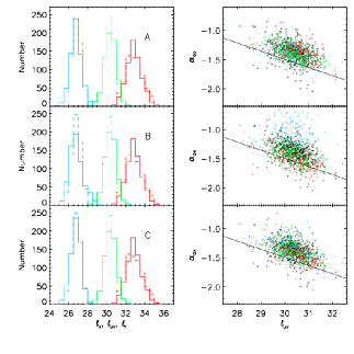
Figure 18.— Simulated populations of RIQs and RLQs compared with the observed primary sample. The models differ principally in the degree of beaming of the jet-linked X-ray emission: A is unbeamed, B is beamed with ${\gamma}_{\rm x}=10.5$ as for the radio jet, and C is beamed to a lesser degree with ${\gamma}_{\rm x}=2.0$. The left-hand side shows histograms of radio (red), optical/UV (green), and X-ray (blue) luminosity, for observations (dashed) and simulation (solid). The right-hand side shows the ${\alpha}_{\rm ox}-{\ell}_{\rm uv}$ relation for the primary sample (black crosses) and for the simulation, with objects color-coded by inclination (blue is $5.8^{\circ}<\theta<10^{\circ}$, green is $10^{\circ}<\theta<20^{\circ}$, and red is $20^{\circ}<\theta<60^{\circ}$). The solid line is the RQQ relation from Just et al. (2007).

It is not possible to leave both the disk/corona and jet-linked X-ray emission as simultaneously free parameters in the absence of additional observational input (such as high-quality X-ray spectra) that most of our sources lack. We assume the X-ray emission associated with the disk/corona is related to the optical disk emission in the same manner as for RQQs (note that this does not necessarily require identical accretion structure) and can therefore be calculated using Equation 7 from Just et al. (2007) and the simulated optical/UV disk emission. Random log normal scatter with $\sigma=0.3$ dex is added to the disk/coronal X-ray luminosities to mimic the scatter in the RQQ relation.

The jet-linked X-ray emission is unlikely to be synchrotron emission from the same population of electrons as generates the radio-jet emission (in contrast to the apparent situation for lower power FR I jets; e.g., Chiaberge et al. 2000), as this process does not appear to generate sufficient X-ray emission to match observations (e.g., Landt et al. 2008). Inverse Compton processes must be considered; sources of seed photons include emission from the jet (self-Compton, or SSC), radiation from the central engine (external Compton, or EC), and the cosmic microwave background (IC/CMB). The IC/CMB model has a strong dependence upon redshift, which conflicts with the lack of redshift dependence observed in our sample (see $\S$5.3), and in any case is unlikely to produce as many seed photons as can the nucleus on the relevant parsec-scale or smaller distances (e.g., Schwartz 2002). Comparison of the SSC and EC processes suggests the latter dominates this close to the central engine (e.g., Sokolov & Marscher 2005).

The precise physical parameters governing X-ray jet emission (such as the size of the emission region or the magnetic-field strength) likely vary significantly from object to object. Since we are interested in general trends rather than the specific details of a given source, we assume a “standard” intrinsic ratio between radio and X-ray jet-linked emission, which we set to obtain consistency with the observed primary sample X-ray luminosities. The intrinsic jet-linked X-ray emission is then modified in models B and C for the observer based on the bulk velocity and inclination of the jet, with presumed dominant EC emission boosted by ${\delta}^{3-2{\alpha}_{\rm x}}$ (an additional factor of $1-\alpha$ beyond the radio synchrotron emission; e.g., Dermer 1995), with ${\alpha}_{\rm x}=-0.3$ for model B taken to match the radio value and ${\alpha}_{\rm x}=-0.5$ for model C taken to match the typical energy index of RLQs (e.g., Page et al. 2005). X-ray censoring is added to the simulated sample in quasi-random fashion, with fainter objects more likely to be labeled as upper limits. For simplicity, this is accomplished through matching the X-ray detection fraction within the top/bottom half of the primary sample ranked by ${\ell}_{\rm x}$. We randomly select 88%/77% of objects with simulated ${\ell}_{\rm x}>26.8/<26.8$ as detections, and then the simulated detection rate matches that of the primary sample overall and within each X-ray luminosity bin.

6.2. Comparison to observed luminosities

In principle, this modeling process will produce a simulated population of RIQs and RLQs that can be directly compared to the observed primary sample data. However, the nature of our sample introduces a few complicating effects that need to be considered. One important parameter is the limiting magnitude for inclusion within the primary sample. Since we prefer to retain as many observed objects as possible, we do not impose a magnitude limit on the observed objects. However, only $\sim$5% of primary sample RIQs and RLQs have $m_{\rm i}>19.95/20.13$ and $m_{\rm i}>20.60/21.08$ for $z<1/z\geq 1$ spectroscopic and photometric quasars, respectively, and so these values are used as effective magnitude cutoffs for the simulations. The numbers of simulated “spectroscopic” and “photometric” objects (distinguished in the model only by the applied magnitude cutoffs) are set to match those of the primary sample.

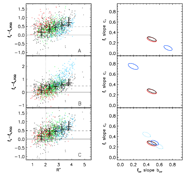
Figure 19.— Simulated populations of RIQs and RLQs compared with the observed primary sample. The models differ principally in the degree of beaming of the jet-linked X-ray emission: A is unbeamed, B is beamed with ${\gamma}_{\rm x}=10.5$ as for the radio jet, and C is beamed to a lesser degree with ${\gamma}_{\rm x}=2.0$. The left-hand side shows “excess” X-ray luminosity relative to comparable RQQs (see Figure 7a) for the observed sample (small black crosses) and for the simulation, with objects color-coded by inclination (blue is $5.8^{\circ}<\theta<10^{\circ}$, green is $10^{\circ}<\theta<20^{\circ}$, and red is $20^{\circ}<\theta<60^{\circ}$). The large black crosses give the median and interquartile range for the primary sample. The right-hand side shows joint 90% confidence ellipses for X-ray luminosity fit as a function of optical/UV and radio luminosity, for the primary sample (red), the full sample (black), and each model (blue). The dotted blue ellipses are for models C1.5 and C3.0 with ${\gamma}_{\rm x}=1.5$ and 3.0. See $\S$6.3 for discussion.

The normalization (i.e., number of objects) of the simulated population should be able to be set solely based on the sky coverage fraction of the observed sample, but this is difficult to evaluate for the various X-ray missions and their complex instrumental fields of view. Matched total numbers of simulated and sample objects are not critical for conducting a comparison (it is the distribution of luminosities that is of interest); nonetheless, it is convenient for examining the results of the simulations if the simulated population is of the same size as the observed sample. Since we are interested in how X-ray luminosity is related to radio and optical/UV luminosities and unconcerned with the sky density of (selected) RIQs and RLQs, we simulate a large population and then draw from it to obtain an equal number of simulated and observed objects. We also simulate variability due to the radio/optical observations being carried out non-simultaneously with the X-ray observations by adding random normal scatter to the simulated ${\ell}_{\rm r}/{\ell}_{\rm uv}$ values (after calculating all interdependent quantities) with amplitudes of 0.0792/0.114 (the same uncertainties as used with fitting; see $\S$5), but inclusion of this minor effect does not significantly impact the modeling.

Another relevant effect is the redshift-dependent efficiency of the SDSS color-selection targeting algorithm and of the photometric quasar classification algorithm. The median redshift of the simulated population is 1.79/1.88 for the spectroscopic/photometric magnitude cutoffs, higher than that of the observed primary sample (for which the median redshift is 1.41). Although the redshift dependencies of quasar color-selection techniques presumably explain most of the discrepancy between the observed and simulated median redshifts, there are a few more factors that could act to decrease the median redshift of the observed primary sample. For example, there is a bias toward lower redshifts for the minority of sources that were X-ray targeted (rather than serendipitous) and a possible bias against spectroscopic identification of fainter objects for which measuring broad emission lines is more difficult. Fortunately, our goal of evaluating X-ray luminosity as a function of radio and optical/UV luminosity does not depend on redshift (e.g., see $\S$5.3), and so it is not necessary to account for all the various selection effects that may influence the difference in redshift distribution. We match in redshift and number simultaneously by drawing from the large simulated population those objects with redshifts close to the observed sample. Note that the underlying basic model could be falsified at this stage were the simulated radio luminosities (specified primarily by the adopted luminosity function, the adopted intrinsic jet/lobe properties, and the random inclination) to disagree with observation. However, a KS test gives a probability of $p=0.21$, indicating that the simulated and observed samples cannot be considered to differ significantly in their radio luminosity distributions. The median radio luminosity for the primary sample is ${\ell}_{\rm r}=32.83$ with a standard deviation of 0.89, while that of the simulated sample is ${\ell}_{\rm r}=32.80$ with a standard deviation of 0.79. It would also be possible at this stage to falsify the nature of the presumed correlation between intrinsic radio jet power and optical/UV disk luminosity if the distribution of simulated optical/UV luminosities were to disagree with observation (the median can always be made to agree by adjusting the ratio, but the distribution reflects the lack of beaming in the optical/UV luminosities, in contrast to the radio). However, a KS test indicates that the simulated and observed samples are not inconsistent ($p=0.41$) in their optical/UV luminosity distributions. The median optical/UV luminosity for the primary sample is ${\ell}_{\rm uv}=30.36$ with a standard deviation of 0.57, while that of the simulated sample is ${\ell}_{\rm uv}=30.33$ with a standard deviation of 0.63. The radio-loudness distributions are also consistent (KS probability $p=0.15$) with observed/simulated median values of 2.50/2.46 and standard deviations of 0.74/0.70. These radio and optical/UV properties are the same for each of models A, B, and C.

For any of models A, B, or C to constitute viable descriptions of the X-ray emission from RIQs and RLQs, it is necessary (but not sufficient) that the distribution of simulated X-ray luminosities not disagree with observation. The X-ray disk/corona emission is completely specified by the optical/UV disk emission, and so it is the additional jet-linked X-ray emission that must be accurately modeled. The median value of the overall simulated X-ray luminosity can always be made to agree with observations by adjusting the ratio between the jet-linked X-ray component and the intrinsic radio-jet luminosity, but the distribution is strongly influenced by the degree to which the jet-linked emission is beamed. The log offsets between intrinsic radio-jet luminosity (prior to applying beaming) and intrinsic X-ray luminosity of the jet-linked component (prior to applying beaming to models B and C) required to match simulated with observed median X-ray luminosities are $-5.35,-7.25,$ and $-7.25$ for models A, B, and C, respectively. Random log-normal scatter is added to these offsets; we find empirically that a somewhat better match to the ${\ell}_{\rm x}$ scatter observed for the primary sample is obtained if the magnitude of this scatter is greater at lower simulated redshifts (0.7/0.3 for $z<1/z\geq 1$), but this could potentially be related to the increased fraction of X-ray bright targeted objects at lower redshifts within the primary sample ($\S$5.4.2), so we do not ascribe physical significance to this result. The X-ray bulk Lorentz factor in model C is ${\gamma}_{\rm x}=2.0$; for reference, this corresponds to ${\delta}_{\rm x}=3.6$ for an inclination of $\theta=5^{\circ}$ (rather than ${\delta}=11.4$ as with the ${\gamma}=10.5$ that applies to the radio jet). For model C, X-ray bulk Lorentz factors of ${\gamma}_{\rm x}\simeq 1-3$ can also match the primary sample X-ray luminosity distributions, but as shown in $\S$6.3, ${\gamma}_{\rm x}=2.0$ produces the best agreement to the observed ${\ell}_{\rm x}({\ell}_{\rm uv},{\ell}_{\rm r})$ relation. KS tests (treating upper limits as detections, but the simulated censoring matches the data) give probabilities of $p=0.37$ and $p=0.30$ for models A and C, respectively, indicating that the simulated and observed samples are not inconsistent in their X-ray luminosity distribution for these models. However, the KS test probability for model B is $p=0.0052$; the simulated distribution of X-ray luminosities differs significantly from that observed. In particular, a tail to large X-ray luminosity values in the simulated population for model B does not agree with the data, which appear to show at most a modest skew toward higher X-ray luminosities (see also $\S$5.4.3). This tail in the model is more pronounced at X-ray than radio frequencies because the dependence upon the $\delta$ beaming factor is greater (by $1-\alpha$ in the exponent) for the X-ray emission. (Model B would be an even worse match to the primary sample if the ${\ell}_{\rm x}$ medians were equalized.) These results may be seen in the left-hand panels of Figure 18.

All three models obviously produce (by design) enhanced X-ray emission relative to RQQs of comparable optical/UV luminosity, as can be seen in the right-hand panels of Figure 18 and as given in Table 10. However, the manner in which they do so differs. In these figures the simulated objects are color-coded by inclination (blue for $5.8^{\circ}<\theta<10^{\circ}$, green for $10^{\circ}<\theta<20^{\circ}$, and red for $20^{\circ}<\theta<60^{\circ}$). For model A, there is essentially no inclination dependence to the X-ray excess, since the X-ray luminosity is unbeamed. For model B, there is a strong inclination dependence, with the lowest inclination RLQs being extremely X-ray bright (to a degree that does not match observations). Note that these simulated low-inclination objects are still expected to be disk-dominated at optical/UV frequencies (as also applies to models A and C) and are thus not blazars, so the comparison to the observed primary sample (from which all identified blazars have been removed) is properly matched. For model C, there is a definite but modest dependence upon inclination. Simultaneous consideration of the distribution of radio, optical/UV, and X-ray luminosities, following the analysis performed in $\S$4 and $\S$5 for observed RIQs and RLQs, provides additional insight helpful to evaluating the feasibility of the three models.

6.3. Modeling results

We now assess the accuracy with which these models (generated as described in $\S$6.1, $\S$6.2, and Table 9) reproduce the observed dependence of X-ray luminosity upon radio and optical/UV luminosities. We first examine how the “excess” X-ray luminosity (X-ray luminosity minus that of a RQQ of matched optical/UV luminosity) for the simulated RIQs and RLQs depends upon radio loudness for the three models. In Figure 19, left-hand side, the simulated objects are again color-coded by inclination, and the primary sample data are plotted along with the median and interquartile range measurements from Figure 7a. It may be observed that model A does not appear to capture accurately the rise in X-ray brightness with increasing radio loudness. This is because in model A the X-ray luminosity is unbeamed, whereas the radio luminosity is beamed, and so the most radio-luminous and radio-loud objects tend to have low inclinations (are color-coded blue) but are not X-ray brighter than higher inclination objects. Conversely, model B overpredicts the degree to which X-ray brightness depends on increasing radio loudness, or inclination. It is only for model C that the X-ray brightness compared to RQQs may be seen to increase with radio loudness in a manner analogous to that observed.

Modeling X-ray luminosity as a joint function of optical/UV and radio luminosity, as done for the observed RIQs and RLQs in $\S$5.2, makes clear the differing manner in which the three models are dependent on optical/UV and radio luminosity (see Table 10). The right-hand side of Figure 19 shows the joint 90% confidence ellipses for the primary (red) and for the full (black) observed samples, along with the calculated result for each model (blue). For model A, the X-ray luminosity is strongly dependent on optical/UV luminosity but only weakly dependent on radio luminosity. The best-fit relation for the population simulated with model A is ${\ell}_{\rm x}=-0.142+0.730\times{\ell}_{\rm uv}+0.100\times{\ell}_{\rm r}$. This result reflects the underlying dependence of both the optical disk emission (and thereby the disk/corona X-ray component) and the “jet-linked” X-ray component on the intrinsic (unbeamed) radio-jet luminosity. The parameterization of X-ray luminosity upon optical/UV and radio luminosity in model A is inconsistent with the fits to the primary and full samples. For model B, the X-ray luminosity is strongly dependent upon radio luminosity but only weakly dependent on optical/UV luminosity. This result is due to the increased dominance of the X-ray continuum by jet-linked emission for a large fraction of the simulated sources, particularly those at low inclinations. The best-fit relation for the population simulated with model B is ${\ell}_{\rm x}=0.099+0.195\times{\ell}_{\rm uv}+0.746\times{\ell}_{\rm r}$. This reflects the mutual beaming of the radio and X-ray jets, but these parameters are also inconsistent with observations. For model C, the X-ray luminosity is dependent upon both optical/UV and radio luminosities in a manner similar to that observed, as illustrated by the overlapping confidence ellipses. The best-fit relation for the population simulated with model C is ${\ell}_{\rm x}=-0.098+0.526\times{\ell}_{\rm uv}+0.279\times{\ell}_{\rm r}$. This result reflects the milder beaming with ${\gamma}_{\rm x}=2.0$ that places model C in some sense intermediate between model A and model B. For comparison, model C with ${\gamma}_{\rm x}=1.5/3.0$ (models C1.5/C3; best-fit relations given in Table 10 and shown as dotted blue ellipses in Figure 19) bracket the ${\gamma}_{\rm x}=2.0$ result but do not provide as close a match to observations.

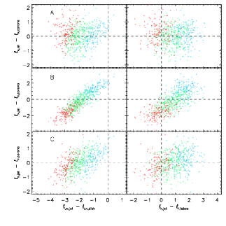
Figure 20.— Simulated populations of RIQs and RLQs. The models differ principally in the degree of beaming of the jet-linked X-ray emission: A is unbeamed, B is beamed with ${\gamma}_{\rm x}=10.5$ as for the radio jet, and C is beamed to a lesser degree with ${\gamma}_{\rm x}=2.0$. In all panels objects are color-coded by inclination (blue is $5.8^{\circ}<\theta<10^{\circ}$, green is $10^{\circ}<\theta<20^{\circ}$, and red is $20^{\circ}<\theta<60^{\circ}$). The left-hand side shows X-ray luminosity components versus optical/UV luminosity components, while the right-hand side shows X-ray luminosity components versus radio luminosity components.

The simulated populations may be utilized to evaluate the dominant emission component at each frequency, and in particular to examine the degree to which X-ray luminosity is dominated by the jet-linked component, as a function of inclination, for the different models (see Figure 20). In nearly all cases, the optical/UV luminosity is disk-dominated. For most sources, and for all the low-inclination sources, the radio luminosity is jet-dominated. In each of models A, B, and C, the X-ray luminosity is dominated by disk/corona emission for a sizeable fraction of objects; there is agreement that despite the greater median X-ray luminosities of RIQs and RLQs relative to RQQs, there are many individual objects for which a disk/corona analogous to that in RQQs is sufficient to produce the majority of observed X-ray emission. For models B and C, the degree to which the X-ray emission is jet-dominated is correlated with the degree to which the radio emission is jet-dominated (to a lesser degree in model C, for which the beaming factor is lower). For the preferred model C, the majority of objects with inclinations less than $20^{\circ}$ have X-ray luminosities dominated by jet-linked emission.

Despite the general nature of the scenarios considered under models A, B, and C, these simulations provide insight into the degree to which the “excess” X-ray luminosity in RIQs and RLQs is jet-linked and beamed. It seems likely that some beaming must be present, as model A does not satisfactorily match observations; this conclusion is consistent with the results of previous work (e.g., Browne & Murphy 1987; Shastri et al. 1993). It also appears that the jet-linked X-ray emission is beamed to a lesser degree than affects the radio jet, as model B does not satisfactorily match observations; this result has also been suggested by other work (e.g., Dou & Yuan 2008). The success of model C suggests that the majority of the jet-linked X-ray emission is not produced cospatially with the radio jet emission, but likely primarily originates in a somewhat slower jet region. The preferred model C implies that high signal-to-noise X-ray spectroscopy of RIQs or RLQs established (e.g., from radio properties) as possessing intermediate inclinations should result in some such objects showing X-ray spectra in which an unabsorbed disk/corona-linked component and a jet-linked component are simultaneously apparent. This is consistent with observational results (although additional X-ray studies would help establish this point); for example, Sambruna et al. (2006) describe three RLQs with concave broken power law X-ray spectra, which they attribute to dual jet/disk-corona components.

Future work with significantly larger samples and denser coverage of the ${\ell}-z$ plane could potentially investigate whether the small-scale jet has velocity structure (as in a fast-spine/slow-sheath model; see, e.g., Jester et al. 2006b), most simply through considering two X-ray jet components with differing bulk Lorentz factors. Modeling deficiencies that are unlikely to impact these results but could be addressed to improve the precision of comparison to data include limited consideration of selection effects and ad-hoc normalization of simulated sample size.

6.4. Alternative model parameters

Although we have not conducted an exhaustive search of the multidimensional parameter space, the presented models (A, B, C, C1.5, and C3.0) together cover a large range of plausible possibilities, and from this set model C best matches observations. It is of interest to evaluate whether a modified set of models would still yield qualitatively similar results. Here, we briefly describe the effects of altering selected model parameters in a reasonable fashion. Minor adjustments to the log offsets between intrinsic radio-jet luminosity and intrinsic jet-linked X-ray luminosity are generally made without comment below; other model parameters are as given in $\S$6.1, $\S$6.2, and Table 9, unless otherwise stated.

The credible interval for $\gamma$ from the adopted Mullin & Hardcastle (2009) model ranges from 3.20 to 14.05. The higher $\gamma$ produces an acceptable match to the primary sample radio and optical/UV luminosities (KS probabilities of 0.59/0.26/0.13 for ${\ell}_{\rm r}/{\ell}_{\rm uv}/R^{*}$) and can match the X-ray luminosity of models A and C but not B (KS probabilities of 0.21/$<0.01$/0.49 for A/B/C). The lower $\gamma$ does not easily give a good match to both the radio and optical/UV luminosities. For a ratio of optical/UV disk emission to unbeamed radio emission of $-2.0$ (logarithmic units) and a minimum inclination of 4^∘, the KS probabilities are 0.059/0.075/0.0076 for ${\ell}_{\rm r}/{\ell}_{\rm uv}/R^{*}$. The simulated median X-ray luminosities may be matched to observations with resulting KS probabilities of 0.35/$<0.01$/0.10 for models A/B/C. In this scenario the majority of the simulated objects have inclinations with ${\theta}>20^{\circ}$, but the X-ray brightness of the lower-inclination objects cause the increase in “excess” X-ray luminosity with increasing radio-loudness for model B and (to a lesser degree) model C to be more rapid than observed. For model C under this scenario, the dependence of X-ray luminosity upon optical/UV and radio luminosity is weaker and stronger ($b_{\rm uv}=0.31$ and $c_{\rm r}=0.55$), respectively, than holds for the primary sample.

Willott et al. (2001) consider two additional models for their radio luminosity function in addition to the version we use (see their $\S$3.2). If instead a population of RIQs and RLQs is simulated based on their model which contains a steeper high-redshift decay (their Equation 11), then an acceptable match to the primary sample may be obtained (KS probabilities of 0.24/0.12/0.42 for ${\ell}_{\rm r}/{\ell}_{\rm uv}/R^{*}$) with a ratio of optical/UV disk emission to unbeamed radio emission of $-1.9$. The KS probabilities for matching simulated versus observed X-ray luminosity are 0.065/$<0.01$/0.35 for models A/B/C. Model B is again not a good match. If instead the Willott et al. (2001) model which becomes constant at high redshift (their Equation 12) is used to simulate a population of RIQs and RLQs, the match to the primary sample is again acceptable (KS probabilities of 0.082/0.19/0.26 for ${\ell}_{\rm r}/{\ell}_{\rm uv}/R^{*}$). The KS probabilities for matching simulated versus observed X-ray luminosity are 0.10/$<0.01$/0.20 for models A/B/C. Model B remains a poor match. Additionally, the median simulated redshift (prior to matching redshifts to the primary sample) is 1.95/2.22 for the spectroscopic/photometric magnitude cutoffs, higher than that of the primary sample (1.41) and also higher than that simulated with the version of the Willott et al. (2001) model we use (1.79/1.88).

We also consider a scenario in which the X-ray jet emission is beamed as ${\delta}^{2-{\alpha}_{\rm x}}$ (similarly to the radio jet emission) rather than as ${\delta}^{3-2{\alpha}_{\rm x}}$. This might apply if, for example, the X-ray jet emission were to be dominated by synchrotron emission from a secondary population of high-energy electrons. This change only affects models B and C. Maintaining ${\alpha}_{\rm x}=-0.3/-0.5$ and adjusting the X-ray jet offsets to $-6.45/-6.50$, the KS probabilities are 0.065/0.76 for models B/C. With less extreme X-ray beaming model B can match the observed distribution of X-ray luminosities. However, model B still predicts a greater fraction of X-ray-bright objects than is observed, and the increase in “excess” X-ray luminosity with increasing radio-loudness is also more rapid than observed. Model C remains a superior explanation of the data. For model C under this scenario, the dependence of X-ray luminosity upon optical/UV and radio luminosity is moderately stronger and weaker ($b_{\rm uv}=0.58$ and $c_{\rm r}=0.23$), respectively, than holds for the primary sample.

7. Summary

The primary results of our analysis of the nuclear X-ray properties of RIQs and RLQs are the following:

1. Sample: We have compiled a sample of 188 RIQs and 603 RLQs (primarily by matching optically selected SDSS quasars to the FIRST survey, taking into account extended radio emission) with high-quality archival X-ray coverage by Chandra, XMM-Newton, or ROSAT. The full sample is almost unbiased with respect to X-ray properties, has a high (85%) detection rate, and can be utilized to investigate the nature and origin of X-ray emission in RIQs and RLQs. The sample size is significantly larger than earlier studies of RLQs and provides superior coverage of the luminosity-redshift plane.

2. Trends: We calculate the ratio of X-ray luminosity in RIQs and RLQs relative to that of comparable RQQs and determine how this ratio increases with both radio loudness and luminosity. This ratio of “excess” X-ray luminosity ranges from $\sim$0.7–2.8 for RIQs through the canonical $\sim$3 for RLQs to $\,\buildrel\scriptstyle>\over{\scriptstyle\sim}\,$10 for strongly radio-loud ($R^{*}>4$) or luminous (${\ell}_{\rm r}>35$) objects. We also carry out fits to the X-ray luminosity as a function of both optical and radio luminosity, which are useful for determining the “typical” X-ray luminosity for any given RIQ or RLQ. The X-ray emission in RIQs is not significantly dependent upon radio luminosity. We quantify the manner in which RLQs become more X-ray luminous for large $R^{*}$ or ${\ell}_{\rm r}$ or for flat radio spectra. Finally, we do not find any significant redshift dependence in the properties of RIQs and RLQs (implying, e.g., that IC/CMB jet-linked emission does not contribute substantially to the nuclear X-ray continuum).

3. Models: We conduct Monte Carlo simulations based on a low-frequency radio luminosity function to which we add a randomly inclined relativistic jet. The optical disk emission is successfully modeled as correlated with the intrinsic (unbeamed) radio-jet luminosity, and the X-ray emission contains both disk/corona and jet-linked components. We consider three models for the non-coronal core X-ray luminosity component, and conclude that the jet-linked X-ray emission is likely beamed but with a lesser bulk Lorentz factor than applies to the radio-jet emission. The alternative possibilities of unbeamed X-ray emission and of X-ray emission with $\gamma\sim 10.5$ as for the radio jet do not appear to match adequately the observed data. For the preferred model, the radio emission is mostly jet dominated, the optical/UV emission is almost exclusively disk dominated, and the X-ray emission is split between disk/corona and jet-linked components with the jet becoming increasingly dominant at low inclinations.

A. Details of primary sample radio/optical/X-ray matching process

We here describe the details of the selection, screening, and matching process used to generate the spectroscopic sample. Many of these steps are identically used in the construction of the photometric sample. Together, the spectroscopic and photometric samples make up the primary sample of RIQs and RLQs used throughout this paper.

The SDSS quasar survey is $\sim$95% complete for unresolved sources (for objects categorized as quasars on the basis of optical spectra) and $\sim$89% complete overall (Vanden Berk et al. 2005); the DR5 quasar catalog of Schneider et al. (2007) consists of quasars with strong broad emission lines (of width $>$1000 km s^-1) and by design does not include BL Lacs with featureless spectra (e.g., Plotkin et al. 2008, 2010). It does, however, include broad-absorption line (BAL) quasars, and it is now clear (e.g., Becker et al. 2000, 2001; Menou et al. 2001) that a small fraction ($\,\buildrel\scriptstyle<\over{\scriptstyle\sim}\,$8% at high radio luminosities; e.g., Shankar et al. 2008) of RLQs have BALs and are, like BAL RQQs, relatively X-ray weak due to intrinsic absorption (e.g., Brotherton et al. 2005; Gibson et al. 2008; Miller et al. 2009). Since we are interested in intrinsic emission and not absorption, we exclude from our sample any objects included in the SDSS BAL catalog of Gibson et al. (2009) and also any RLQs we are aware of as possessing BALs not observable in the SDSS spectrum (e.g., J100726.10+124856.2, the $z=0.24$ object PG 1004+130 identified as a BAL RLQ by Wills et al. 1999). Through this process 22 BAL quasars are identified and dropped from further consideration. Contamination from low-redshift ($z<1.7$) RLQs not identifiable as having BALs due to SDSS bandpass limitations (e.g., spectroscopic quasars lacking coverage of the 1400–1550 Å region, which includes the strong C IV BAL transition) is estimated to be $\sim$2% of the entire sample, and a small number of X-ray weak outliers would not materially impact our results below. Objects with apparent heavy intrinsic reddening are sometimes also associated with X-ray absorption (e.g., Hall et al. 2006). The quantity ${\Delta}(g-i)$ (plotted in Figure 2) is the $g-i$ color of an object (corrected for Galactic extinction) less the median $g-i$ quasar color at the redshift of that object; negative ${\Delta}(g-i)$ values correspond to objects bluer than the norm and positive ${\Delta}(g-i)$ values indicate redder colors (e.g., Richards et al. 2001). For reference, the median relative color for our sample of spectroscopic SDSS RIQs and RLQs is ${\Delta}(g-i)=0.07$ (there is a general tendency for RLQs to have somewhat redder colors than RQQs; e.g., Labita et al. 2008). Almost all non-reddened objects have ${\Delta}(g-i)<1$ while intrinsically reddened (and potentially absorbed) objects form a tail in the distribution that extends past this value (e.g., Hall et al. 2006), so objects with ${\Delta}(g-i)>1$ are culled from the sample. This cut removes 8 objects that would otherwise be included (an additional 4 of the already excluded BAL quasars also have ${\Delta}(g-i)>1$). Finally, 3 objects possess radio spectra (described in $\S$3.3) indicating they are GHz-peaked spectrum (GPS; e.g., O’Dea 1998) sources, which are generally considered to be young sources and have X-ray properties that are not necessarily representative of RLQs in general (e.g., Siemiginowska et al. 2008); these GPS sources are therefore culled and not considered further.

Extended radio sources (with jets or lobes) may have separate entries in the FIRST source catalog for each detected component, and lobe-dominated sources do not always possess a detected core component. It is therefore necessary to match to the entire environment surrounding each quasar to recover all associated emission (e.g., Best et al. 2005; Lu et al. 2007). Very few radio sources that lack a core component have lobe-to-lobe angular sizes greater than 90^′′ (e.g., de Vries et al. 2006), so we search for radio emission within 90^′′ of each optically-selected quasar. We considered as candidates for radio-detected quasars those objects with a radio source within 2^′′, referred to hereafter as the core, or two or more radio sources within 2${}^{\prime\prime}<\theta<90^{\prime\prime}$ of which at least one pair has component angular orientations relative to the core differing by more than 90^∘ (where a 180^∘ separation would indicate components on directly opposite sides of the core), classified as potential lobes pending additional review. The potential lobes were then matched to the SDSS photometric catalog, and if they had an optical counterpart (unless that apparent counterpart was a spectroscopically-classified star) they were flagged as intruding background sources and not considered further in determining the radio characteristics of that quasar; if this process left only one potential lobe and no core then the object was eliminated as not radio-detected. All objects with remaining potential lobes were then examined visually to screen further for misclassifications (for example, unrelated background double-lobed radio sources are readily identifiable by eye as intruding but are difficult to categorize correctly automatically). A few cases in which an obviously-associated extended component had been mistakenly flagged as background due to a randomly coincident SDSS optical source were also corrected. Visual screening also identified four objects with likely associated radio components outside the 90^′′ consideration radius (J093200.08+553347.4, J112956.53+364919.2, J094745.14+072520.6, and J142735.60+263214.5, with maximal lobe offset from the core of 93^′′, 99^′′, 117^′′, and 148^′′, respectively); since we wish to take into account all lobe emission from objects already included in the sample, these components were added to the total radio fluxes for these objects. Visual screening also confirmed that the FIRST catalog contains entries for all obvious components in all sources included in the sample [with only one exception: we added a core component to J170441.37+604430.5 (3C 351) based on examination of the FIRST and other radio maps]. The FIRST survey is not particularly sensitive to large-scale regions of low surface brightness, so diffuse lobes may not be detected or may have their fluxes underestimated (e.g., Lu et al. 2010). The NRAO VLA Sky Survey (NVSS; Condon et al. 1998) provides lower angular resolution coverage that complements the high angular resolution imaging of FIRST; 1.4 GHz fluxes from the NVSS catalog were used for a handful of obviously extended FIRST sources.

The 312 RIQs and RLQs in the spectroscopic sample all possess sensitive X-ray coverage from Chandra, XMM-Newton, or ROSAT. For Chandra, we checked all public non-grating ACIS-S or ACIS-I observations with exposures longer than 1 ks and off-axis angles of less than 12^′ (note that each one of the ACIS CCDs covers an area of approximately 8.4^′ by 8.4^′). For XMM-Newton, we considered only those observations with exposure times greater than 1 ks and off-axis angles of less than 15^′. For ROSAT, we initially considered unfiltered PSPC observations with exposure times greater than 2 ks and off-axis angles less than 40^′. All X-ray observations were examined to screen out cases in which the quasar did not fall on the detector, was too close to another bright source, was located within an instrumental artifact, or was otherwise unsuitable for further analysis. Due to their greater X-ray sensitivity, Chandra or XMM-Newton observations were prioritized over ROSAT observations. In cases where both Chandra and XMM-Newton provide coverage, the observation with the greatest X-ray signal-to-noise ratio (estimated based on exposure time, off-axis angle, detector efficiency, and average background) was used. ROSAT observations were ranked by X-ray signal-to-noise ratio, and lower-quality observations were discarded. The threshold value for discarding ROSAT observations was chosen so as to provide a large sample size while maintaining a relatively high detection fraction. In cases where multiple ROSAT observations were available, the observation with the greatest X-ray signal-to-noise ratio was used. Despite their lower sensitivity, the ROSAT observations are useful for this project, as they provide a large area of sky coverage beyond that available solely from Chandra and XMM-Newton observations. Note that this method is unbiased with respect to intrinsic quasar properties (including X-ray brightness) as it is based only on the expected quality of the X-ray observations, so it should not lead to any biases or systematic errors in our analyses.

B. Using GALEX data to improve photometric redshifts

We here describe the process through which GALEX observations were used to identify and discard 34 RIQs and RLQs with likely incorrect photometric redshifts and a further 25 objects for which the accuracy of the photometric redshifts could not be checked (see also $\S$2.1.2).

Out of the 406 photometric RIQs and RLQs under consideration prior to incorporation of GALEX data, 151 (37%) have $z_{\rm phot}>1.9$, of which 121 have GALEX coverage. From these 121, we use a color-color cut and a joint-detection cut to identify 43 objects with questionable photometric redshifts. For these 43 objects, 37/29/23 (86%/67%/53%) are flagged by the color-color/joint-detection/both methods (so 14/6, or 33%/14%, are flagged exclusively by the color-color/joint-detection method). From these 43 objects, 9 have spectroscopic redshifts (in all cases confirming the photometric redshift was incorrect) and are retained with corrected redshifts and luminosities. The remaining 34 objects are discarded. Of the 30 objects with $z_{\rm phot}>1.9$ lacking GALEX coverage, 5 have spectroscopic redshifts (in all cases indicating the photometric redshift is correct); the remaining 25 objects are conservatively discarded, sacrificing some completeness to minimize potential contamination. Additional details are provided below.

The color-color index $(m_{\rm NUV}-m_{\rm r})-2.5(m_{\rm g}-m_{\rm r})$ cleanly separates $z_{\rm spec}\leq 1$ from $z_{\rm spec}\geq 1.9$ objects (D. W. Hogg 2009, personal communication). We flag the 37 objects with photometric redshifts $z_{\rm phot}\geq 1.9$ but $(m_{\rm NUV}-m_{\rm r})-2.5(m_{\rm g}-m_{\rm r})<1.5$, of which we estimate $\sim$31 are actually low-redshift quasars. From the catalog of SDSS DR3 quasars matched to GALEX data provided by Trammell et al. (2007), of the quasars with both FUV and NUV detections the fraction with $z_{\rm spec}>1.9$ is 6.9% (or 7.7%/8.6% for objects with $m_{\rm i}>19/20$; the median $m_{\rm i}$ for the photometric sample is 20.0). In contrast, within the primary sample, $\simeq$23% of the quasars with both FUV and NUV detections have $z_{\rm phot}\geq 1.9$. We flag the 29 objects with NUV and FUV detections and $z_{\rm phot}\geq 1.9$, of which we estimate $\sim$18 are actually low-redshift quasars. Most (23/29) of the objects with both FUV and NUV detections are already flagged for rejection by the color-color cut, so this process finds 6 new objects with questionable photometric redshifts. After combining methods we generate a rejection list of 43 objects with photometric redshifts $z\geq 1.9$ but GALEX properties more characteristic of low-redshift quasars; we estimate $\sim$(30–35)/43 are indeed low-redshift, and only $\sim$10% of genuine $z\geq 1.9$ quasars are lost through these cuts. The GALEX detection rate of low-redshift SDSS quasars is sufficiently high (Trammell et al. 2007) that virtually all interlopers with GALEX coverage are expected to be identifiable through this process.

We checked the rejection list of 43 objects (with photometric redshifts $z\geq 1.9$ but GALEX properties more characteristic of low-redshift quasars) for SDSS DR6 or NED spectroscopic coverage, finding 9 objects with spectroscopic redshifts available for comparison. From these, 7 objects have incorrect photometric redshifts $z\geq 1.9$ but spectroscopic redshifts $z\leq 1$ (of which 6/5/4 objects were flagged for rejection by color-color/joint-detection/both cuts.) The other 2 objects also have (less dramatically) incorrect photometric redshifts, with spectroscopic redshifts $\sim$0.5 below the photometric estimate (these objects are flagged for rejection by both methods). No objects with spectroscopically confirmed photometric redshifts of $z>1.9$ are on this rejection list. We correct the redshifts (and luminosities) of these 9 objects with spectroscopic coverage and then remove them from the rejection list, which therefore consists of 34 objects. Of the 30 objects with photometric redshifts $z\geq 1.9$ that lack GALEX coverage, 5 also have spectroscopic redshifts and are retained, while the remaining 25 (of which $\sim$7 are likely actually low-redshift) are conservatively added to the rejection list. After discarding objects on the rejection list, the updated candidate list of photometric RIQs and RLQs contains 347 ($=406-34-25$) objects, within which the remaining fraction with this type of redshift misindentification is only $\sim$1.5%.

C. Notes on individual deep-field objects

Here we present brief commentary on selected RIQs and RLQs from the CDF-N and the E-CDF-S; the interested reader is referred to the provided references for additional detail.

123538.51+621643.0 is included in the XMM-Newton Bright Serendipitous Survey (Della Ceca et al. 2004). Galbiati et al. (2005) describe it as a non-blazar AGN (with $R^{*}=1.22$ and ${\alpha}_{\rm r}=2.5$ calculated from 1.4 to 8.5 GHz) and find that the X-ray spectrum can be adequately fit by a power-law model with $\Gamma=1.96^{+0.08}_{-0.05}$ and no intrinsic absorption.

123649.62+620737.8 is near the borderline of our X-ray hardness-ratio cut and may be mildly obscured, although it is nevertheless relatively X-ray bright. It is classified as a type-2 AGN by, e.g., Padovani et al. (2004), using the definition of Szokoly et al. (2004). Trouille et al. (2008) characterize the optical spectrum as showing high excitation lines (i.e., not an obvious broad-line object), but its ${\Delta}(g-i)$ value is $-0.17$, bluer than the typical quasar at that redshift.

123746.63+621739.0 is listed in the radio catalog of Richards et al. (1998) as having a radio flux density of 11.1 $\mu$Jy at 8.5 GHz, and is also in the radio catalog of Richards et al. (1999) with a flux density of 998 $\mu$Jy at 1.4 GHz, in agreement with the flux density from Biggs & Ivison (2006). The optical counterpart has quasar-like colors but lacks an optical spectrum that would permit definitive classification.

033115.03$-$275518.5 has a lobe-dominated radio morphology and shows double-peaked optical broad-line emission structure. Details may be found in Luo et al. (2009).

033124.86$-$275207.1 has two other optical objects within $2.5^{\prime\prime}$, but the selected counterpart is secure. It is described in Rovilos et al. (2007) as a type-1 AGN based on its soft X-ray spectrum.

033139.49$-$274119.6 is listed in the ACTA radio catalog of Norris et al. (2006) as having a 1.4 GHz flux density of 0.2 mJy, in agreement with the flux density of 206 $\mu$Jy from Miller et al. (2008). This object is detected in the Spitzer Wide-Area Infrared Extragalactic Survey (Lonsdale et al. 2003) and has optical quasar-like colors but lacks an optical spectrum that would permit definitive classification.

033208.66$-$274734.4 is a bright RIQ with a broad-line optical spectrum (e.g., Tozzi et al. 2009). Lehmer et al. (2005) describe the X-ray spectrum (containing $\sim$20000 counts) as having an effective photon index of $\Gamma=1.73$ (calculated from the hardness ratio), and Steffen et al. (2006) quote a radio-loudness of $R^{*}=1.14$.

033210.91$-$274414.9 is a RLQ with a broad-line optical spectrum (e.g., Tozzi et al. 2009). Wang et al. (2007) find that the X-ray spectrum (containing $\sim$1000 counts) can be well-fit by a power-law model with $\Gamma=1.88\pm 0.09$ and no intrinsic absorption.

033211.63$-$273725.9 has COMBO-17 colors consistent with those of a template quasar spectrum. Lehmer et al. (2005) describe the X-ray spectrum as having an effective photon index of $\Gamma=1.44$ (calculated from the hardness ratio), and Steffen et al. (2006) quote a radio-loudness of $R^{*}=1.29$. This source is detected in the Spitzer Wide-Area Infrared Extragalactic Survey.

033227.01$-$274105.0 is a broad-line quasar (e.g., Tozzi et al. 2009). Galbiati et al. (2005) quote $R^{*}=2.05$ and ${\alpha}_{\rm r}=-0.53$ and fit the X-ray spectrum with a power-law plus blackbody model ($\Gamma=2.04\pm 0.15$ and $kT=0.15\pm 0.06$) with no intrinsic absorption.

D. Verification of fitting methodology

We fit X-ray luminosity as a function of various parameters using the IDL code of Kelly (2007), which takes into account censoring of the dependent variable and uncertainties in all variables. This is an advance over methods that consider either censoring (e.g., ASURV) or errors (e.g., the IDL program fitexy) but not both simultaneously. Here, we illustrate the fitting technique through application to the RQQ sample of Steffen et al. (2006), for which results using an alternative method (ASURV) have already been reported.

In this sample of RQQs the uncertainties are dominated by intrinsic variability (see, e.g., $\S$3.5 of Gibson et al. 2008), as is also the case for the RIQs and RLQs that form the primary focus of this work. The uncertainties we use throughout are based on observed data, but we investigate here the degree to which the fitting results are sensitive to alternative values for the uncertainties. Figure 21a shows ${\ell}_{\rm x}({\ell}_{\rm uv})$ computed for RQQs for our standard errors (solid line), for a fit resulting from doubling the standard errors (dashed line), and for a fit resulting from halving the standard errors (dotted line). The coefficients for the standard error fit are ${\ell}_{\rm x}=(-0.545\pm 0.023)+(0.649\pm 0.021)\times{\ell}_{\rm uv}$; for the double errors fit they are ${\ell}_{\rm x}=(-0.540\pm 0.023)+(0.673\pm 0.022)\times{\ell}_{\rm uv}$; for the half errors fit they are ${\ell}_{\rm x}=(-0.546\pm 0.023)+(0.644\pm 0.021)\times{\ell}_{\rm uv}$. When comparing the coefficient values it must be kept in mind that these coefficients are probabilistically derived, so a large number of fits would be required to quantify most accurately the impact of using different error values. However, it is clear that varying the uncertainties within reasonable bounds does not dramatically alter the parameters of the best-fit line (i.e., the credible intervals of the parameters overlap).

Figure 21.— Demonstration of fitting methodology for ${\ell}_{\rm x}({\ell}_{\rm uv})$ applied to RQQs. The top panel illustrates that varying the uncertainties in the variables within a reasonable range has only a minimal impact upon the best-fit correlation. The bottom panel shows that using the code of Kelly (2007) provides results consistent with those given by ASURV, and illustrates the effect of considering ${\ell}_{\rm uv}$ rather than ${\ell}_{\rm x}$ as the dependent variable, or of using the bisector line. See Appendix D for details.

The best-fit model obtained through using the Kelly (2007) code agrees with that calculated by Steffen et al. (2006) using ASURV and treating ${\ell}_{\rm x}$ as the dependent variable (their Equation 1a), which is ${\ell}_{\rm x}=(-0.546\pm 0.023)+(0.642\pm 0.021)\times{\ell}_{\rm uv}$ using our normalization convention. As described in $\S$5.1, it seems reasonable on both practical and statistical grounds to consider ${\ell}_{\rm x}$ as the dependent variable throughout. However, other approaches are possible; we investigate the effect of considering ${\ell}_{\rm uv}$ as the dependent variable and of using the bisector best-fit line. When fitting ${\ell}_{\rm uv}({\ell}_{\rm x})$ and inverting the results, the slope will generally be steeper than for the fit conducted with ${\ell}_{\rm x}$ as the dependent variable. A complicating factor is that it is no longer possible to consider the censoring in ${\ell}_{\rm x}$. However, treating all upper limits as X-ray detections, we find ${\ell}_{\rm x}=-0.475+0.812\times{\ell}_{\rm uv}$, which may be compared with the Steffen et al. (2006) result (their Equation 1b) of ${\ell}_{\rm x}=-0.400+0.815\times{\ell}_{\rm uv}$. For reference, the best-fit lines calculated using the IDL program fitexy are ${\ell}_{\rm x}=-0.500+0.695\times{\ell}_{\rm uv}$ and ${\ell}_{\rm x}=-0.491+0.736\times{\ell}_{\rm uv}$ treating ${\ell}_{\rm x}$ and ${\ell}_{\rm uv}$ in turn as the dependent variable. Calculating the bisector using Table 1 of Isobe et al. (1990) gives ${\ell}_{\rm x}=-0.493+0.727\times{\ell}_{\rm uv}$ for our fits, or ${\ell}_{\rm x}=-0.478+0.721\times{\ell}_{\rm uv}$ from Steffen et al. (2006; their Equation 1c). The bisector slope is slightly higher, but it may be seen in Figure 21b that the change in the distance from the best-fit line for any given point is at most $\sim$0.2 over the span of the variables. When we discuss “outliers” or “positive residuals” we are referring to greater distances from the best-fit line. We note that the best-fit lines may not always appear to run through the highest density of points when upper limits are present; for example, the RIQ fit to ${\ell}_{\rm x}({\ell}_{\rm uv})$ in Figure 9a may appear different than would be the case were all of the upper limits detections.

As a final consistency check, we also performed every fit given in Table 7 with ASURV. In all cases, the parameters agreed (in the sense that the 1$\sigma$ intervals overlapped) with those computed using the code of Kelly (2007). The median differences between the best-fit parameters obtained using the code of Kelly (2007) and those obtained with ASURV (and the standard deviations thereof) for the ${\ell}_{\rm x}({\ell}_{\rm uv})$ model are $-0.0009~{}(0.0085)$ for $a_{\rm 0}$ and $0.0262~{}(0.0082)$ for $b_{\rm uv}$; without considering the uncertainties, ASURV apparently computes slightly flatter slopes for these datasets (recall that the typical values for $b_{\rm uv}$ are 0.6–0.8 in these fits, so this systematic difference is 3–4%). The median differences (and standard deviations) for the ${\ell}_{\rm x}({\ell}_{\rm uv},{\ell}_{\rm r})$ model are $0.0006~{}(0.0049)$ for $a_{\rm 0}$, $0.0200~{}(0.0130)$ for $b_{\rm uv}$, and $-0.0088~{}(0.0094)$ for $c_{\rm r}$. For illustrative purposes, if the Kelly (2007) code is run with an uncertainty on ${\ell}_{\rm uv}$ of 0.05 rather than 0.114 (keeping the uncertainties on ${\ell}_{\rm r}$ and ${\ell}_{\rm x}$ at 0.0792 and 0.146), the average change in $b_{\rm uv}/c_{\rm r}$ is $-0.022/0.0079$, producing coefficients matching the ASURV results (with a similar impact on $b_{\rm uv}$ in the ${\ell}_{\rm x}({\ell}_{\rm uv})$ relation).

We conclude that using only ${\ell}_{\rm x}$ as the dependent variable is acceptable for our comparative study and that using the IDL code of Kelly (2007) to take both censoring and uncertainties into account is advantageous.

Table 1Primary sample RIQs and RLQs

Name	$z$	$m_{\rm i}$	${\Delta}(g-i)$	${\ell}_{\rm r}$	${\ell}_{\rm uv}$	${\ell}_{\rm x}$	Det	$R^{*}$	${\alpha}_{\rm ox}$	${\alpha}_{\rm r}$	${\ell}_{\rm r,core}$	SDSS	X-ray
000442.18$+$000023.3	1.008	19.02	$-$0.02	31.92	30.28	26.91	1	1.64	$-$1.30	0.00	31.92	S	X
000622.60$-$000424.4	1.038	19.49	0.21	34.97	30.05	27.29	1	4.91	$-$1.06	$-$0.72	34.97	S	C
001130.40$+$005751.8	1.492	20.08	$-$0.05	33.96	30.13	27.17	1	3.84	$-$1.13	$-$0.22	33.96	S	X
004230.40$-$092202.7	2.085	19.97	0.01	34.01	30.51	26.31	1	3.50	$-$1.61	0.00	34.01	P	c
004413.72$+$005141.0	0.941	18.44	0.06	32.64	30.42	26.61	1	2.22	$-$1.46	0.00	$<$31.29	S	X
005009.81$-$003900.6	0.728	19.89	0.63	31.68	29.36	26.25	1	2.32	$-$1.20	0.00	31.68	S	C
005905.50$+$000651.6	0.719	17.46	$-$0.07	34.42	30.62	27.37	1	3.80	$-$1.24	$-$0.40	34.42	S	C
012401.76$+$003500.9	1.850	20.23	0.26	34.12	30.26	26.90	1	3.86	$-$1.29	$-$0.70	34.12	S	C
012528.84$-$000555.9	1.077	16.47	$-$0.09	34.59	31.36	27.73	1	3.23	$-$1.39	0.22	34.59	S	r
012734.57$-$000523.8	1.598	20.37	0.14	33.32	30.04	26.74	1	3.28	$-$1.27	0.00	33.32	S	r

Note. — Table 1 is provided in its entirety in the online edition of the journal. A portion is shown here for guidance as to its form and content. Some values here and in the following tables are given to precision greater than the uncertainty to avoid future accumulated round-off error.

Table 2RIQs and RLQs selected from deep surveys

Name	$z$	$m_{\rm i}$	${\ell}_{\rm r}$	${\ell}_{\rm uv}$	${\ell}_{\rm x}$	$R^{*}$	${\alpha}_{\rm ox}$	Ref
Color selected
033115.03$-$275518.5	1.368	21.43	32.71	29.60	26.48	3.11	$-$1.20	1
033124.86$-$275207.1	1.328	21.09	33.18	29.31	25.72	3.87	$-$1.38
033139.49$-$274119.6	2.215	23.12	31.36	29.29	$<$25.04	2.06	$<-$1.63
033208.66$-$274734.4	0.543	18.78	31.03	29.26	25.94	1.77	$-$1.27	2
033210.91$-$274414.9	1.605	22.95	32.26	29.10	26.08	3.16	$-$1.16	3
033211.63$-$273725.9	1.636	18.99	32.36	30.72	26.85	1.64	$-$1.49
033227.01$-$274105.0	0.737	19.09	32.31	29.95	26.34	2.36	$-$1.39	3
033302.67$-$274823.1	3.021	23.96	31.38	29.31	26.51	2.06	$-$1.08
033310.20$-$274841.9	1.034	22.66	32.68	28.58	25.71	4.10	$-$1.10	3
123529.38$+$621256.4	2.413	23.21	31.24	29.37	26.11	1.88	$-$1.25	5
123538.51$+$621643.0	0.712	19.70	31.50	29.53	26.50	1.97	$-$1.16	5
123649.62$+$620737.8	1.610	23.51	31.25	28.85	26.17	2.40	$-$1.03	6
123746.63$+$621739.0	2.316	23.36	32.12	29.25	$<$25.20	2.87	$<-$1.56
095958.54$+$015254.6	1.019	21.86	31.02	28.56	24.80	2.46	$-$1.44
100046.92$+$020726.6	1.210	21.70	31.81	28.97	25.37	2.85	$-$1.38
100114.86$+$020208.9	0.969	20.63	31.97	29.31	26.00	2.66	$-$1.27	8
Broad-line selected
033225.17$-$274218.8	1.617	23.37	30.70	28.82	25.78	1.87	$-$1.17	4
123704.11$+$620755.4	1.253	22.07	30.44	29.11	25.54	1.32	$-$1.37	7
123707.51$+$622148.0	1.451	23.04	30.45	28.92	26.20	1.53	$-$1.04	7
095821.65$+$024628.2	1.403	19.05	32.36	30.48	26.75	1.88	$-$1.43	8
095838.47$+$022439.3	1.161	21.86	30.34	28.71	26.23	1.63	$-$0.95	8
095908.32$+$024309.6	1.317	18.43	33.32	30.66	27.16	2.66	$-$1.35	8
095921.31$+$024412.4	1.004	20.46	31.57	29.42	25.53	2.15	$-$1.49	8
100114.86$+$020208.8	0.969	21.00	31.97	29.27	26.18	2.70	$-$1.19	8
100129.83$+$023239.0	0.826	20.54	30.36	28.80	25.54	1.55	$-$1.25	8
100205.03$+$023731.5	0.519	19.05	30.68	29.25	26.23	1.43	$-$1.16	8
100213.42$+$023351.7	1.143	21.76	30.25	28.94	25.68	1.32	$-$1.25	8
100228.82$+$024016.9	3.144	21.27	31.56	29.69	26.76	1.87	$-$1.12	8
100230.06$+$014810.4	0.626	19.65	30.22	28.30	25.51	1.92	$-$1.07	8
100240.93$+$023448.4	1.677	21.98	30.74	29.35	25.89	1.40	$-$1.33	8
100249.33$+$023746.5	2.124	19.75	32.84	30.62	26.37	2.22	$-$1.63	8

Table 3Sample characteristics

	X-ray sources				Median properties
Sample	$N$	$N_{\rm det}$	100$\frac{N_{\rm det}}{N}$		$z$	${\ell}_{\rm r}$	${\ell}_{\rm uv}$	${\ell}_{\rm x}$	$R^{*}$	${\alpha}_{\rm ox}$
Full, primary, and supplemental samples
Full	791	674	85		1.40	32.95	30.42	26.79	2.59	$-$1.40
Primary	654	547	84		1.41	32.83	30.36	26.73	2.50	$-$1.40
Spectroscopic	312	274	88		1.32	33.00	30.49	26.83	2.46	$-$1.41
QSO/HIZ	200	186	93		1.20	33.14	30.67	26.97	2.50	$-$1.41
Photometric	342	273	80		1.47	32.72	30.23	26.64	2.52	$-$1.39
Off-axis	562	456	81		1.45	32.73	30.33	26.70	2.44	$-$1.40
Targeted	92	91	99		1.05	33.65	30.74	27.04	3.09	$-$1.39
Supplemental	137	127	93		1.32	34.33	30.96	27.38	3.11	$-$1.36
Einstein	93	85	91		1.02	34.63	31.15	27.55	3.44	$-$1.39
High-$z$	13	13	100		4.31	34.69	31.42	27.70	2.90	$-$1.34
Deep fields	31	29	94		1.32	31.50	29.27	26.04	2.06	$-$1.26
FIRST	180	164	91		1.27	33.16	30.73	26.99	2.41	$-$1.43
RIQs and RLQs
RIQs	188	142	76		1.42	32.05	30.41	26.50	1.67	$-$1.50
RLQs	603	532	88		1.38	33.30	30.44	26.89	2.88	$-$1.37
Groupings of RLQs
$R^{*}<3$	343	291	85		1.42	32.87	30.34	26.69	2.47	$-$1.41
$R^{*}\geq 3$	260	241	93		1.33	34.08	30.59	27.16	3.46	$-$1.31
${\ell}_{\rm r}<33.3$	301	251	83		1.26	32.68	30.11	26.53	2.50	$-$1.37
${\ell}_{\rm r}\geq 33.3$	302	281	93		1.63	34.04	30.82	27.22	3.31	$-$1.37
${\alpha}_{\rm r}<-0.5$	181	160	88		1.31	33.59	30.48	26.93	3.18	$-$1.38
${\alpha}_{\rm r}\geq-0.5$	221	207	94		1.26	33.66	30.61	27.11	3.10	$-$1.34

Note. — The columns $N$, $N_{\rm det}$, and 100$\frac{N_{\rm det}}{N}$ give the number of sources, the number of X-ray detected sources, and the percentage of sources with X-ray detections, respectively. Radio, optical/UV, and X-ray monochromatic luminosities ${\ell}_{\rm r}$, ${\ell}_{\rm uv}$, and ${\ell}_{\rm x}$ are expressed as logarithmic quantities with units of erg s^-1 Hz^-1 at rest-frame 5 GHz, 2500 Å, and 2 keV, respectively. The radio loudness is $R^{*}={\ell}_{\rm r}-{\ell}_{\rm uv}$ and the optical/UV-to-X-ray spectral slope is ${\alpha}_{\rm ox}=0.384\times({\ell}_{\rm x}-{\ell}_{\rm uv})$. RIQs have $1{\leq}R^{*}$$<2$ and RLQs have $R^{*}\geq 2$. Medians that include limits were determined with ASURV. Details regarding the various samples are given in $\S$2.

Table 4RIQ and RLQ properties as a function of ${\ell}_{\rm uv}$

	${\ell}_{\rm uv}$ bin range
Statistic	$<$29.5	29.5–30	30–30.5	30.5–31	31–31.5	$\geq$31.5
X-ray sources
$N$	69	119	257	210	92	44
$N_{\rm det}$	57	98	217	176	86	40
100$\frac{N_{\rm det}}{N}$	83	82	84	84	93	91
Redshift
Mean	0.87	1.04	1.36	1.72	2.09	2.71
25th %	0.47	0.74	1.05	1.09	1.27	2.01
50th %	0.71	1.03	1.39	1.70	1.99	2.44
75th %	1.15	1.33	1.69	2.20	2.90	3.52
${\ell}_{\rm uv}$
Mean	29.12	29.80	30.27	30.73	31.21	31.78
25th %	28.85	29.67	30.16	30.61	31.11	31.60
50th %	29.27	29.82	30.28	30.73	31.19	31.73
75th %	29.38	29.92	30.40	30.85	31.31	31.91
${\ell}_{\rm x}$
Mean	25.77	26.35	26.67	26.97	27.52	27.83
25th %	25.38	26.06	26.42	26.72	27.27	27.48
50th %	25.75	26.38	26.72	27.03	27.53	27.71
75th %	26.23	26.57	26.94	27.21	27.78	28.13
${\alpha}_{\rm ox}$
Mean	$-$1.28	$-$1.32	$-$1.39	$-$1.45	$-$1.42	$-$1.52
25th %	$-$1.46	$-$1.43	$-$1.46	$-$1.52	$-$1.53	$-$1.62
50th %	$-$1.25	$-$1.32	$-$1.38	$-$1.44	$-$1.42	$-$1.54
75th %	$-$1.16	$-$1.25	$-$1.28	$-$1.34	$-$1.31	$-$1.45
$R^{*}$
Mean	2.66	2.52	2.51	2.67	2.96	2.67
25th %	1.92	2.03	1.97	2.06	2.33	2.19
50th %	2.66	2.43	2.47	2.64	3.14	2.77
75th %	3.27	2.90	3.01	3.37	3.71	3.24

Note. — Properties here are for the full sample of RIQs and RLQs. Quantities and units are as defined in Table 3. The ${\ell}_{\rm uv}$ bins are plotted in Figure 3.

Table 5Excess X-ray luminosity as a function of $R^{*}$ and ${\ell}_{\rm r}$: full sample

	$R^{*}$ bin range					${\ell}_{\rm r}$ bin range
Statistic	$<$2.0	2.0–2.5	2.5–3.0	3.0–3.5	$\geq 3.5$		$<32.2$	32.2–32.9	32.9–33.6	33.6–34.3	$\geq 34.3$
$N$	188	175	168	141	119		176	198	187	108	122
$N_{\rm det}$	142	145	146	128	113		138	156	163	102	115
100$\frac{N_{\rm det}}{N}$	76	83	87	91	95		78	79	87	94	94
${\ell}_{\rm x}-{\ell}_{\rm x,RQQ}$
Mean	0.11	0.29	0.41	0.58	0.77		0.22	0.22	0.42	0.55	0.76
Error	0.04	0.03	0.03	0.03	0.05		0.04	0.04	0.03	0.04	0.04
25th %	$-$0.16	0.08	0.26	0.35	0.53		$-$0.13	0.05	0.22	0.34	0.51
50th %	0.16	0.30	0.44	0.57	0.71		0.29	0.29	0.41	0.53	0.67
75th %	0.45	0.52	0.62	0.77	1.03		0.59	0.52	0.62	0.72	0.94
$R^{*}$
Mean	1.62	2.26	2.75	3.25	3.85		1.88	2.27	2.77	3.15	3.61
Error	0.02	0.01	0.01	0.01	0.03		0.04	0.04	0.04	0.05	0.04
25th %	1.42	2.14	2.62	3.11	3.62		1.52	1.88	2.50	2.88	3.35
50th %	1.67	2.28	2.74	3.25	3.78		1.86	2.29	2.79	3.20	3.65
75th %	1.86	2.39	2.88	3.38	4.00		2.14	2.58	3.07	3.48	3.87
${\ell}_{\rm r}$
Mean	31.98	32.62	33.14	33.75	34.38		31.69	32.54	33.23	33.91	34.77
Error	0.05	0.05	0.05	0.06	0.07		0.03	0.01	0.01	0.02	0.03
25th %	31.56	32.17	32.79	33.34	33.93		31.44	32.36	33.07	33.72	34.46
50th %	32.05	32.58	33.18	33.70	34.51		31.82	32.54	33.23	33.92	34.72
75th %	32.36	32.95	33.47	34.23	34.94		32.03	32.70	33.39	34.06	34.97

Note. — The “excess” X-ray luminosity is defined as ${\ell}_{\rm x}-{\ell}_{\rm x,RQQ}$, where ${\ell}_{\rm x,RQQ}=0.709{\ell}_{\rm uv}+4.822$ from Just et al. (2007). Other quantities and units are as defined in Table 3. Note that the first $R^{*}$ bin is the sample of RIQs. The inner bins in $R^{*}$ increase by linear factors of $\sim$3; the inner bins in ${\ell}_{\rm r}$ increase by linear factors of $\sim$5. These values are plotted in Figure 7.

Table 6Excess X-ray luminosity as a function of $R^{*}$ and ${\ell}_{\rm r}$: primary sample

	$R^{*}$ bin range					${\ell}_{\rm r}$ bin range
Statistic	$<$2.0	2.0–2.5	2.5–3.0	3.0–3.5	$\geq 3.5$		$<32.2$	32.2–32.9	32.9–33.6	33.6–34.3	$\geq 34.3$
$N$	171	154	147	111	71		154	187	172	90	51
$N_{\rm det}$	125	126	128	102	66		118	145	150	84	50
100$\frac{N_{\rm det}}{N}$	73	82	87	92	93		77	78	87	93	98
${\ell}_{\rm x}-{\ell}_{\rm x,RQQ}$
Mean	0.07	0.30	0.42	0.56	0.67		0.20	0.21	0.44	0.54	0.70
Error	0.04	0.03	0.03	0.03	0.06		0.04	0.04	0.03	0.04	0.04
25th %	$-$0.20	0.12	0.26	0.34	0.53		$-$0.13	0.03	0.23	0.34	0.52
50th %	0.13	0.30	0.44	0.54	0.65		0.23	0.29	0.41	0.53	0.65
75th %	0.41	0.52	0.62	0.74	0.97		0.57	0.52	0.63	0.71	0.87
$R^{*}$
Mean	1.62	2.26	2.74	3.25	3.82		1.86	2.25	2.77	3.21	3.66
Error	0.02	0.01	0.01	0.01	0.03		0.04	0.04	0.04	0.05	0.05
25th %	1.41	2.14	2.61	3.12	3.61		1.51	1.87	2.50	2.95	3.45
50th %	1.67	2.28	2.74	3.25	3.77		1.84	2.28	2.80	3.27	3.70
75th %	1.84	2.39	2.87	3.38	3.92		2.11	2.56	3.07	3.49	3.85
${\ell}_{\rm r}$
Mean	32.06	32.57	33.08	33.58	34.09		31.78	32.54	33.23	33.89	34.61
Error	0.04	0.04	0.04	0.06	0.09		0.03	0.01	0.02	0.02	0.04
25th %	31.69	32.17	32.76	33.26	33.66		31.55	32.36	33.07	33.70	34.38
50th %	32.07	32.54	33.13	33.61	34.32		31.87	32.52	33.22	33.90	34.57
75th %	32.38	32.92	33.41	34.04	34.67		32.04	32.70	33.39	34.04	34.74

Note. — Quantities defined as in Table 5.

Table 7Correlations with X-ray luminosity

	${\ell}_{\rm x}=a_{\rm 0}+b_{\rm uv}\times{\ell}_{\rm uv}$			${\ell}_{\rm x}=a_{\rm 0}+b_{\rm uv}\times{\ell}_{\rm uv}+c_{\rm r}\times{\ell}_{\rm r}$
Sample	$a_{\rm 0}$	$b_{\rm uv}$		$a_{\rm 0}$	$b_{\rm uv}$	$c_{\rm r}$
Full, primary, and supplemental samples
Full	$-$0.144${}^{+0.017}_{-0.016}$	0.789${}^{+0.026}_{-0.025}$		$-$0.098${}^{+0.014}_{-0.015}$	0.482${}^{+0.031}_{-0.031}$	0.273${}^{+0.019}_{-0.019}$
Primary	$-$0.190${}^{+0.018}_{-0.018}$	0.721${}^{+0.031}_{-0.031}$		$-$0.116${}^{+0.016}_{-0.016}$	0.480${}^{+0.033}_{-0.034}$	0.263${}^{+0.021}_{-0.021}$
Spectroscopic	$-$0.193${}^{+0.024}_{-0.024}$	0.640${}^{+0.042}_{-0.043}$		$-$0.103${}^{+0.021}_{-0.020}$	0.380${}^{+0.041}_{-0.042}$	0.296${}^{+0.025}_{-0.024}$
QSO/HIZ	$-$0.168${}^{+0.030}_{-0.030}$	0.651${}^{+0.049}_{-0.048}$		$-$0.088${}^{+0.025}_{-0.025}$	0.400${}^{+0.048}_{-0.047}$	0.294${}^{+0.030}_{-0.031}$
Photometric	$-$0.162${}^{+0.027}_{-0.028}$	0.816${}^{+0.050}_{-0.048}$		$-$0.111${}^{+0.026}_{-0.027}$	0.611${}^{+0.057}_{-0.058}$	0.214${}^{+0.035}_{-0.034}$
Off-axis	$-$0.208${}^{+0.020}_{-0.020}$	0.744${}^{+0.036}_{-0.036}$		$-$0.123${}^{+0.019}_{-0.020}$	0.528${}^{+0.039}_{-0.040}$	0.243${}^{+0.023}_{-0.025}$
Targeted	$-$0.039${}^{+0.045}_{-0.043}$	0.553${}^{+0.064}_{-0.065}$		$-$0.089${}^{+0.035}_{-0.037}$	0.335${}^{+0.059}_{-0.059}$	0.320${}^{+0.044}_{-0.044}$
Supplemental	$+$0.028${}^{+0.044}_{-0.044}$	0.823${}^{+0.045}_{-0.044}$		$-$0.017${}^{+0.041}_{-0.041}$	0.491${}^{+0.079}_{-0.079}$	0.253${}^{+0.051}_{-0.052}$
Einstein	$+$0.039${}^{+0.072}_{-0.075}$	0.793${}^{+0.087}_{-0.087}$		$-$0.233${}^{+0.072}_{-0.077}$	0.472${}^{+0.089}_{-0.090}$	0.407${}^{+0.066}_{-0.068}$
FIRST	$-$0.196${}^{+0.035}_{-0.034}$	0.668${}^{+0.062}_{-0.063}$		$-$0.098${}^{+0.028}_{-0.030}$	0.409${}^{+0.060}_{-0.059}$	0.297${}^{+0.032}_{-0.032}$
RQQs, RIQs, and RLQs
RQQs	$-$0.545${}^{+0.023}_{-0.023}$	0.649${}^{+0.021}_{-0.021}$		$\cdots$	$\cdots$	$\cdots$
RIQs	$-$0.447${}^{+0.037}_{-0.038}$	0.567${}^{+0.056}_{-0.057}$		$-$0.477${}^{+0.212}_{-0.215}$	0.588${}^{+0.181}_{-0.178}$	$-$0.025${}^{+0.175}_{-0.177}$
RLQs	$-$0.057${}^{+0.017}_{-0.017}$	0.831${}^{+0.026}_{-0.025}$		$-$0.100${}^{+0.016}_{-0.016}$	0.506${}^{+0.037}_{-0.038}$	0.292${}^{+0.027}_{-0.026}$
Groupings of RLQs
$R^{*}<3$	$-$0.191${}^{+0.020}_{-0.020}$	0.771${}^{+0.032}_{-0.032}$		$-$0.149${}^{+0.032}_{-0.032}$	0.620${}^{+0.100}_{-0.100}$	0.144${}^{+0.088}_{-0.091}$
$R^{*}\geq 3$	$+$0.112${}^{+0.026}_{-0.025}$	0.844${}^{+0.036}_{-0.034}$		$-$0.177${}^{+0.057}_{-0.058}$	0.432${}^{+0.081}_{-0.085}$	0.398${}^{+0.073}_{-0.070}$
${\ell}_{\rm r}<33.3$	$-$0.180${}^{+0.032}_{-0.032}$	0.739${}^{+0.045}_{-0.046}$		$-$0.098${}^{+0.040}_{-0.040}$	0.610${}^{+0.061}_{-0.062}$	0.205${}^{+0.065}_{-0.065}$
${\ell}_{\rm r}\geq 33.3$	$+$0.070${}^{+0.028}_{-0.028}$	0.687${}^{+0.045}_{-0.044}$		$-$0.170${}^{+0.034}_{-0.035}$	0.439${}^{+0.047}_{-0.048}$	0.389${}^{+0.040}_{-0.040}$
${\alpha}_{\rm r}<-0.5$	$-$0.091${}^{+0.023}_{-0.023}$	0.652${}^{+0.045}_{-0.045}$		$-$0.175${}^{+0.025}_{-0.025}$	0.363${}^{+0.061}_{-0.061}$	0.259${}^{+0.041}_{-0.041}$
${\alpha}_{\rm r}\geq-0.5$	$+$0.066${}^{+0.029}_{-0.029}$	0.800${}^{+0.039}_{-0.040}$		$-$0.041${}^{+0.026}_{-0.026}$	0.471${}^{+0.052}_{-0.050}$	0.342${}^{+0.039}_{-0.040}$

Note. — Fitting is done with the IDL code of Kelly (2007), which utilizes Bayesian techniques that incorporate both errors and upper limits. Errors are assumed to be dominated by intrinsic random flux variability; see, e.g., $\S 3.5$ of Gibson et al. (2008). The luminosities are normalized prior to fitting as ${\ell}_{\rm r}-33.3,{\ell}_{\rm uv}-30.5,{\ell}_{\rm x}-27.0$. For any given model fit the quoted parameter values are the median of draws from the posterior distribution and the errors are 1$\sigma$. These results are plotted in Figures 9–13.

Table 8${\alpha}_{\rm ox}$ and ${\Delta}{\alpha}_{\rm ox}$ as functions of $R^{*}$

Sample	N	$z$	$R^{*}$	${\alpha}_{\rm ox}/{\Delta}{\alpha}_{\rm ox}$	Intercept $a$	Slope $b$
${\alpha}_{\rm ox}=a+b\times{R^{*}}$
$z<1$	213	0.69	2.68	$-$1.33	$-$1.556${}^{+0.043}_{-0.043}$	0.079${}^{+0.015}_{-0.015}$
$1<z<2$	406	1.44	2.54	$-$1.39	$-$1.653${}^{+0.029}_{-0.029}$	0.101${}^{+0.011}_{-0.011}$
$z>2$	172	2.49	2.56	$-$1.49	$-$1.862${}^{+0.048}_{-0.048}$	0.152${}^{+0.017}_{-0.017}$
${\Delta}{\alpha}_{\rm ox}=a+b\times{R^{*}}$
$z<1$	213	0.69	2.68	0.18	$-$0.101${}^{+0.040}_{-0.041}$	0.097${}^{+0.014}_{-0.014}$
$1<z<2$	406	1.44	2.54	0.17	$-$0.118${}^{+0.027}_{-0.027}$	0.106${}^{+0.010}_{-0.010}$
$z>2$	172	2.49	2.56	0.16	$-$0.234${}^{+0.047}_{-0.048}$	0.155${}^{+0.017}_{-0.017}$

Note. — Fitting as described for Table 7. Uncertainties for the fitting were propagated from those assumed for luminosities.

Table 9Description of model components

Parameter	Value	Comment
$z$	Quasi-random	From W01 RLF, then use values close to primary sample to account for redshift selection effects.
$\theta$	Random	Drawn from uniform distribution in $\sin{\theta}$.
${\theta}_{\rm min}$	$5.8^{\circ\dagger}$	Minimum permitted inclination; values between $4^{\circ}-7^{\circ}$ are viable.
Radio
$\rho$, ${\sigma}_{\rm\rho}$, $\gamma$	$-5.61,1.38,10.49$	From Table 5 of MH09. Both $\rho$ and ${\sigma}_{\rm\rho}$ are expressed as natural logs.
${\ell}_{\rm r,lobes}$	Random	From W01 RLF, then shifted to 5 GHz using ${\alpha}_{\rm r}=-0.9$
${\ell}_{\rm r,jet0}$	Calculated	${\ell}_{\rm r,jet0}$ from ${\ell}_{\rm r,lobes}$ and $\rho$ with scatter from ${\sigma}_{\rm\rho}$.
${\ell}_{\rm r,jet}$	Calculated	${\ell}_{\rm r,jet}$ = ${\ell}_{\rm r,jet0}\times{\delta}^{2-{\alpha}_{\rm r}}$, $\delta={\gamma}^{-1}(1-\beta\cos{\theta})^{-1}$, ${\alpha}_{\rm r}=-0.3$.
$f_{\rm r,min}$	1, 2.7 mJy	Flux density limit at 1.4 GHz for core (FIRST 5$\sigma$), effective limit for lobes ($\lower 2.0pt\hbox{$\,\buildrel\scriptstyle<\over{\scriptstyle\sim}\,$}5$% of lobes below).
Optical
${\rho}_{\rm dj0}$, ${\sigma}_{\rm dj0}$	$-1.8^{\dagger},0.5$	Logarithmic ratio of disk to intrinsic (unbeamed) radio jet; correlation motivated by W99 results.
${\ell}_{\rm uv,disk}$	Calculated	${\ell}_{\rm uv,disk}={\ell}_{\rm r,jet0}+{\rho}_{\rm dj0}$ with scatter from ${\sigma}_{\rm dj0}$
${\ell}_{\rm uv,jet}$	Calculated	Extrapolated from ${\ell}_{\rm r,jet}$ using ${\alpha}_{\rm ro}=-0.8$. Observations restrict optical jet flux.
$m_{\rm i,max}$	19.95/20.13, 20.60/21.08	Cutoff $m_{\rm i}$ for $z<1/z\geq 1$; from depth ($\lower 2.0pt\hbox{$\,\buildrel\scriptstyle<\over{\scriptstyle\sim}\,$}5$% objects above) of spectroscopic, photometric samples.
X-ray
${\ell}_{\rm x,corona}$	Calculated	Determined from ${\ell}_{\rm uv,disk}$ following the RQQ relation of J07.
${\rho}_{\rm j,A}$, ${\rho}_{\rm j,B}$, ${\rho}_{\rm j,C}$	$-5.35^{\dagger},-7.25^{\dagger},-7.25^{\dagger}$	Logarithmic ratio of X-ray jet-linked emission to intrinsic radio jet for models A, B, and C.
${\sigma}_{\rm dx},{\sigma}_{\rm j}$	0.3, $0.7^{\dagger}/0.3^{\dagger}$	Scatter in ${\ell}_{\rm x,corona}$ (from RQQ ${\ell}_{\rm x}({\ell}_{\rm uv})$ relation) and in ${\rho}_{\rm j}$ for $z<1/z\geq 1$ for models A, B, and C.
${\gamma}_{\rm x,A}$, ${\gamma}_{\rm x,B}$, ${\gamma}_{\rm x,C}$	1.0, 10.49, 2.0†	Bulk Lorentz factor governing beaming of X-ray jet-linked emission for models A, B, and C.
${\ell}_{\rm x,jet}$	Calculated	Determined from ${\ell}_{\rm r,jet0}$ and ${\rho}_{\rm j}$, with boosting of ${\delta}_{\rm x}^{3-2{\alpha}_{\rm x}}$, ${\alpha}_{\rm x}=-0.3/-0.5$ for B/C.

Note. — See $\S$6 for modeling details.

Table 10Model X-ray luminosities and ${\ell}_{\rm x}({\ell}_{\rm uv},{\ell}_{\rm r})$

	X-ray luminosities				${\ell}_{\rm x}=a_{\rm 0}+b_{\rm uv}\times{\ell}_{\rm uv}+c_{\rm r}\times{\ell}_{\rm r}$
Sample	${\ell}_{\rm x}$	$\sigma$	KS $p$		$a_{\rm 0}$	$b_{\rm uv}$	$c_{\rm r}$
Primary	26.80	0.54	$\cdots$		$-0.116^{+0.016}_{-0.016}$	$0.480^{+0.033}_{-0.034}$	$0.263^{+0.021}_{-0.021}$
Model A	26.74	0.58	0.37		$-0.142^{+0.016}_{-0.017}$	$0.730^{+0.030}_{-0.029}$	$0.100^{+0.022}_{-0.022}$
Model B	26.72	0.75	$<0.01$		$+0.099^{+0.020}_{-0.020}$	$0.195^{+0.035}_{-0.035}$	$0.746^{+0.027}_{-0.027}$
Model C	26.75	0.55	0.30		$-0.098^{+0.016}_{-0.016}$	$0.526^{+0.028}_{-0.027}$	$0.279^{+0.021}_{-0.021}$
Model C1.5	26.78	0.55	0.76		$-0.105^{+0.017}_{-0.016}$	$0.593^{+0.028}_{-0.029}$	$0.210^{+0.022}_{-0.022}$
Model C3.0	26.78	0.59	0.10		$-0.000^{+0.016}_{-0.017}$	$0.400^{+0.028}_{-0.028}$	$0.435^{+0.022}_{-0.022}$

Note. — Models are described in $\S$6. Fitting as described in Table 7. Upper limits are included in the simulated sample at a rate consistent with those observed in the primary sample.

References

- Adelman-McCarthy et al. (2007) Adelman-McCarthy, J. K., et al. 2007, ApJS, 172, 634
- Alexander et al. (2003) Alexander, D. M., et al. 2003, AJ, 126, 539
- Antonucci (1993) Antonucci, R. 1993, ARA&A, 31, 473
- Avni & Tananbaum (1986) Avni, Y., & Tananbaum, H. 1986, ApJ, 305, 83
- Barthel (1989) Barthel, P. D. 1989, ApJ, 336, 606
- Baldwin (1977) Baldwin, J. A. 1977, ApJ, 214, 679
- Barger et al. (2003) Barger, A. J., et al. 2003, AJ, 126, 632
- Barger et al. (2007) Barger, A. J., Cowie, L. L., & Wang, W.-H. 2007, ApJ, 654, 764
- Barger et al. (2008) Barger, A. J., Cowie, L. L., & Wang, W.-H. 2008, ApJ, 689, 687
- Bassett et al. (2004) Bassett, L. C., Brandt, W. N., Schneider, D. P., Vignali, C., Chartas, G., & Garmire, G. P. 2004, AJ, 128, 523
- Becker et al. (1995) Becker, R. H., White, R. L., & Helfand, D. J. 1995, ApJ, 450, 559
- Becker et al. (2000) Becker, R. H., White, R. L., Gregg, M. D., Brotherton, M. S., Laurent-Muehleisen, S. A., & Arav, N. 2000, ApJ, 538, 72
- Becker et al. (2001) Becker, R. H., et al. 2001, ApJS, 135, 227
- Bell & Comeau (2010) Bell, M. B., & Comeau, S. P. 2010, Ap&SS, 325, 31
- Belsole et al. (2006) Belsole, E., Worrall, D. M., & Hardcastle, M. J. 2006, MNRAS, 366, 339
- Best et al. (2005) Best, P. N., Kauffmann, G., Heckman, T. M., & Ivezić, Ž. 2005, MNRAS, 362, 9
- Biggs & Ivison (2006) Biggs, A. D., & Ivison, R. J. 2006, MNRAS, 371, 963
- Blundell & Kuncic (2007) Blundell, K. M., & Kuncic, Z. 2007, ApJ, 668, L103
- Brandt & Alexander (2010) Brandt, W. N., & Alexander, D. M. 2010, Proceedings of the National Academy of Science, 107, 7184
- Brinkmann et al. (1997) Brinkmann, W., Yuan, W., & Siebert, J. 1997, A&A, 319, 413
- Brotherton et al. (2005) Brotherton, M. S., Laurent-Muehleisen, S. A., Becker, R. H., Gregg, M. D., Telis, G., White, R. L., & Shang, Z. 2005, AJ, 130, 2006
- Browne & Murphy (1987) Browne, I. W. A., & Murphy, D. W. 1987, MNRAS, 226, 601
- Capak et al. (2007) Capak, P., et al. 2007, ApJS, 172, 99
- Cappelluti et al. (2009) Cappelluti, N., et al. 2009, A&A, 497, 635
- Cappi et al. (1997) Cappi, M., Matsuoka, M., Comastri, A., Brinkmann, W., Elvis, M., Palumbo, G. G. C., & Vignali, C. 1997, ApJ, 478, 492
- Chiaberge et al. (2000) Chiaberge, M., Capetti, A., & Celotti, A. 2000, A&A, 355, 873
- Cirasuolo et al. (2003) Cirasuolo, M., Celotti, A., Magliocchetti, M., & Danese, L. 2003, MNRAS, 346, 447
- Coleman et al. (1980) Coleman, G. D., Wu, C.-C., & Weedman, D. W. 1980, ApJS, 43, 393
- Condon et al. (1998) Condon, J. J., Cotton, W. D., Greisen, E. W., Yin, Q. F., Perley, R. A., Taylor, G. B., & Broderick, J. J. 1998, AJ, 115, 1693
- Della Ceca et al. (2004) Della Ceca, R., et al. 2004, A&A, 428, 383
- Dermer (1995) Dermer, C. D. 1995, ApJ, 446, L63
- Donoso et al. (2009) Donoso, E., Best, P. N., & Kauffmann, G. 2009, MNRAS, 392, 617
- Dou & Yuan (2008) Dou, L.-M., & Yuan, W.-M. 2008, Chinese Journal of Astronomy and Astrophysics, 8, 653
- Douglas et al. (1996) Douglas, J. N., Bash, F. N., Bozyan, F. A., Torrence, G. W., & Wolfe, C. 1996, AJ, 111, 1945
- Elvis et al. (2009) Elvis, M., et al. 2009, ApJS, 184, 158
- Evans et al. (2006) Evans, D. A., Worrall, D. M., Hardcastle, M. J., Kraft, R. P., & Birkinshaw, M. 2006, ApJ, 642, 96
- Evans et al. (2008) Evans, I. N., Evans, J. D., Fabbiano, G., Glotfelty, K. J., McCollough, M. L., McDowell, J. C., Primini, F. A., & Rots, A. H. 2008, Proceedings of the SPIE, 7016, 53
- Falcke et al. (1996) Falcke, H., Sherwood, W., & Patnaik, A. R. 1996, ApJ, 471, 106
- Fanaroff & Riley (1974) Fanaroff, B. L., & Riley, J. M. 1974, MNRAS, 167, 31P
- Galbiati et al. (2005) Galbiati, E., et al. 2005, A&A, 430, 927
- Garofalo et al. (2010) Garofalo, D., Evans, D. A., & Sambruna, R. M. 2010, MNRAS, 406, 975
- Gawiser et al. (2006) Gawiser, E., et al. 2006, ApJS, 162, 1
- Gehrels (1986) Gehrels, N. 1986, ApJ, 303, 336
- Giacconi et al. (2002) Giacconi, R., et al. 2002, ApJS, 139, 369
- Gibson et al. (2008) Gibson, R. R., Brandt, W. N., & Schneider, D. P. 2008, ApJ, 685, 773
- Gibson et al. (2009) Gibson, R. R., et al. 2009, ApJ, 692, 758
- Gopal-Krishna & Wiita (2000) Gopal-Krishna, & Wiita, P. J. 2000, A&A, 363, 507
- Green et al. (2009) Green, P. J., et al. 2009, ApJ, 690, 644
- Gregory et al. (1996) Gregory, P. C., Scott, W. K., Douglas, K., & Condon, J. J. 1996, ApJS, 103, 427
- Haardt & Maraschi (1991) Haardt, F., & Maraschi, L. 1991, ApJ, 380, L51
- Hall et al. (2006) Hall, P. B., Gallagher, S. C., Richards, G. T., Alexander, D. M., Anderson, S. F., Bauer, F., Brandt, W. N., & Schneider, D. P. 2006, AJ, 132, 1977
- Hardcastle et al. (2009) Hardcastle, M. J., Evans, D. A., & Croston, J. H. 2009, MNRAS, 396, 1929
- Hasinger (2008) Hasinger, G. 2008, A&A, 490, 905
- Ilbert et al. (2008) Ilbert, O., et al. 2008, Astronomical Society of the Pacific Conference Series, 399, 169
- Ilbert et al. (2009) Ilbert, O., et al. 2009, ApJ, 690, 1236
- Isobe & Feigelson (1990) Isobe, T., & Feigelson, E. D. 1990, BAAS, 22, 917
- Ivezić et al. (2002) Ivezić, Ž., et al. 2002, AJ, 124, 2364
- Ivezić et al. (2004) Ivezić, Z., et al. 2004, Astronomical Society of the Pacific Conference Series, 311, 347
- Jackson & Wall (1999) Jackson, C. A., & Wall, J. V. 1999, MNRAS, 304, 160
- Jester et al. (2005) Jester, S., et al. 2005, AJ, 130, 873
- Jester et al. (2006a) Jester, S., Körding, E., & Fender, R. 2006a, VI Microquasar Workshop: Microquasars and Beyond, 1, 26
- Jester et al. (2006b) Jester, S., Harris, D. E., Marshall, H. L., & Meisenheimer, K. 2006b, ApJ, 648, 900
- Jiang et al. (2007) Jiang, L., Fan, X., Ivezić, Ž., Richards, G. T., Schneider, D. P., Strauss, M. A., & Kelly, B. C. 2007, ApJ, 656, 680
- Just et al. (2007) Just, D. W., Brandt, W. N., Shemmer, O., Steffen, A. T., Schneider, D. P., Chartas, G., & Garmire, G. P. 2007, ApJ, 665, 1004
- Kaspi et al. (2007) Kaspi, S., Brandt, W. N., Maoz, D., Netzer, H., Schneider, D. P., & Shemmer, O. 2007, ApJ, 659, 997
- Kellermann et al. (1989) Kellermann, K. I., Sramek, R., Schmidt, M., Shaffer, D. B., & Green, R. 1989, AJ, 98, 1195
- Kellermann et al. (2008) Kellermann, K. I., Fomalont, E. B., Mainieri, V., Padovani, P., Rosati, P., Shaver, P., Tozzi, P., & Miller, N. 2008, ApJS, 179, 71
- Kelly (2007) Kelly, B. C. 2007, ApJ, 665, 1489
- Kelly et al. (2007) Kelly, B. C., Bechtold, J., Siemiginowska, A., Aldcroft, T., & Sobolewska, M. 2007, ApJ, 657, 116
- Kraft et al. (1991) Kraft, R. P., Burrows, D. N., & Nousek, J. A. 1991, ApJ, 374, 344
- Labita et al. (2008) Labita, M., Treves, A., & Falomo, R. 2008, MNRAS, 383, 1513
- Landt et al. (2008) Landt, H., Padovani, P., Giommi, P., Perri, M., & Cheung, C. C. 2008, ApJ, 676, 87
- Laor (2000) Laor, A. 2000, ApJ, 543, L111
- Laor & Behar (2008) Laor, A., & Behar, E. 2008, MNRAS, 390, 847
- Lehmer et al. (2005) Lehmer, B. D., et al. 2005, ApJS, 161, 21
- Lonsdale et al. (2003) Lonsdale, C. J., et al. 2003, PASP, 115, 897
- Lopez et al. (2006) Lopez, L. A., Brandt, W. N., Vignali, C., Schneider, D. P., Chartas, G., Garmire, G. P. 2006, AJ, 131, 1914
- Lu et al. (2007) Lu, Y., Wang, T., Zhou, H., & Wu, J. 2007, AJ, 133, 1615
- Lu et al. (2010) Lu, Y., Wang, T., Zhou, H., & Wu, J. 2010, arXiv:1002.0636
- Luo et al. (2008) Luo, B., et al. 2008, ApJS, 179, 19
- Luo et al. (2009) Luo, B., et al. 2009, ApJ, 695, 1227
- Luo et al. (2010) Luo, B., et al. 2010, ApJS, 187, 560
- Lynden-Bell (1969) Lynden-Bell, D. 1969, Nature, 223, 690
- Mackay (1971) Mackay, C. D. 1971, MNRAS, 154, 209
- Maoz (2007) Maoz, D. 2007, MNRAS, 377, 1696
- Marshall et al. (2005) Marshall, H. L., et al. 2005, ApJS, 156, 13
- Martin et al. (2005) Martin, D. C., et al. 2005, ApJ, 619, L1
- McGreer et al. (2009) McGreer, I. D., Helfand, D. J., & White, R. L. 2009, AJ, 138, 1925
- Meier (2001) Meier, D. L. 2001, ApJ, 548, L9
- Menou et al. (2001) Menou, K., et al. 2001, ApJ, 561, 645
- Metcalf & Magliocchetti (2006) Metcalf, R. B., & Magliocchetti, M. 2006, MNRAS, 365, 101
- Mignoli et al. (2005) Mignoli, M., et al. 2005, A&A, 437, 883
- Miller et al. (1993) Miller, P., Rawlings, S., & Saunders, R. 1993, MNRAS, 263, 425
- Miller et al. (2008) Miller, N. A., Fomalont, E. B., Kellermann, K. I., Mainieri, V., Norman, C., Padovani, P., Rosati, P., & Tozzi, P. 2008, ApJS, 179, 114
- Miller et al. (2009) Miller, B. P., Brandt, W. N., Gibson, R. R., Garmire, G. P., & Shemmer, O. 2009, ApJ, 702, 911
- Mullin & Hardcastle (2009) Mullin, L. M., & Hardcastle, M. J. 2009, MNRAS, 398, 1989
- Norris et al. (2006) Norris, R. P., et al. 2006, AJ, 132, 2409
- O’Dea (1998) O’Dea, C. P. 1998, PASP, 110, 493
- Orr & Browne (1982) Orr, M. J. L., & Browne, I. W. A. 1982, MNRAS, 200, 1067
- Osmer & Shields (1999) Osmer, P. S., & Shields, J. C. 1999, Astronomical Society of the Pacific Conference Series, 162, 235
- Padovani et al. (2004) Padovani, P., Allen, M. G., Rosati, P., & Walton, N. A. 2004, A&A, 424, 545
- Page et al. (2005) Page, K. L., Reeves, J. N., O’Brien, P. T., & Turner, M. J. L. 2005, MNRAS, 364, 195
- Plotkin et al. (2008) Plotkin, R. M., Anderson, S. F., Hall, P. B., Margon, B., Voges, W., Schneider, D. P., Stinson, G., & York, D. G. 2008, AJ, 135, 2453
- Plotkin et al. (2010) Plotkin, R. M., et al. 2010, AJ, 139, 390
- Rafferty et al. (2010) Rafferty, D. A., Brandt, W. N., Alexander, D.M. , Xue, Y. Q., Bauer, F. E., Lehmer, B. D., Luo, B., & Papovich, C. 2010, ApJ, submitted
- Rawlings & Saunders (1991) Rawlings, S., & Saunders, R. 1991, Nature, 349, 138
- Rees & Setti (1968) Rees, M. J., & Setti, G. 1968, Nature, 219, 127
- Rengelink et al. (1997) Rengelink, R. B., Tang, Y., de Bruyn, A. G., Miley, G. K., Bremer, M. N., Roettgering, H. J. A., & Bremer, M. A. R. 1997, A&AS, 124, 259
- Richards et al. (1998) Richards, E. A., Kellermann, K. I., Fomalont, E. B., Windhorst, R. A., & Partridge, R. B. 1998, AJ, 116, 1039
- Richards et al. (1999) Richards, E. A., Fomalont, E. B., Kellermann, K. I., Windhorst, R. A., Partridge, R. B., Cowie, L. L., & Barger, A. J. 1999, ApJ, 526, L73
- Richards et al. (2001) Richards, G. T., et al. 2001, AJ, 121, 2308
- Richards et al. (2002) Richards, G. T., et al. 2002, AJ, 123, 2945
- Richards et al. (2009) Richards, G. T., et al. 2009, ApJS, 180, 67
- Rovilos et al. (2007) Rovilos, E., Georgakakis, A., Georgantopoulos, I., Afonso, J., Koekemoer, A. M., Mobasher, B., & Goudis, C. 2007, A&A, 466, 119
- Sambruna et al. (2004) Sambruna, R. M., Gambill, J. K., Maraschi, L., Tavecchio, F., Cerutti, R., Cheung, C. C., Urry, C. M., & Chartas, G. 2004, ApJ, 608, 698
- Sambruna et al. (2006) Sambruna, R. M., Gliozzi, M., Tavecchio, F., Maraschi, L., & Foschini, L. 2006, ApJ, 652, 146
- Scheuer (1995) Scheuer, P. A. G. 1995, MNRAS, 277, 331
- Schinnerer et al. (2007) Schinnerer, E., et al. 2007, ApJS, 172, 46
- Schneider et al. (2007) Schneider, D. P., et al. 2007, AJ, 134, 102
- Schwartz (2002) Schwartz, D. A. 2002, ApJ, 569, L23
- Shankar et al. (2008) Shankar, F., Dai, X., & Sivakoff, G. R. 2008, ApJ, 687, 859
- Shankar et al. (2010) Shankar, F., Sivakoff, G. R., Vestergaard, M., & Dai, X. 2010, MNRAS, 401, 1869
- Shastri et al. (1993) Shastri, P., Wilkes, B. J., Elvis, M., & McDowell, J. 1993, ApJ, 410, 29
- Shields (1978) Shields, G. A. 1978, Nature, 272, 706
- Siemiginowska et al. (2008) Siemiginowska, A., LaMassa, S., Aldcroft, T. L., Bechtold, J., & Elvis, M. 2008, ApJ, 684, 811
- Sokolov & Marscher (2005) Sokolov, A., & Marscher, A. P. 2005, ApJ, 629, 52
- Spergel et al. (2007) Spergel, D. N., et al. 2007, ApJS, 170, 377
- Steffen et al. (2006) Steffen, A. T., Strateva, I., Brandt, W. N., Alexander, D. M., Koekemoer, A. M., Lehmer, B. D., Schneider, D. P., & Vignali, C. 2006, AJ, 131, 2826
- Stocke et al. (1992) Stocke, J. T., Morris, S. L., Weymann, R. J., & Foltz, C. B. 1992, ApJ, 396, 487
- Strateva et al. (2005) Strateva, I. V., Brandt, W. N., Schneider, D. P., Vanden Berk, D. G., & Vignali, C. 2005, AJ, 130, 387
- Suchkov et al. (2006) Suchkov, A. A., Hanisch, R. J., Voges, W., & Heckman, T. M. 2006, AJ, 132, 1475
- Szokoly et al. (2004) Szokoly, G. P., et al. 2004, ApJS, 155, 271
- Tavecchio et al. (2000) Tavecchio, F., Maraschi, L., Sambruna, R. M., & Urry, C. M. 2000, ApJ, 544, L23
- Tavecchio et al. (2007) Tavecchio, F., Maraschi, L., Ghisellini, G., Kataoka, J., Foschini, L., Sambruna, R. M., & Tagliaferri, G. 2007, ApJ, 665, 980
- Tozzi et al. (2009) Tozzi, P., et al. 2009, ApJ, 698, 740
- Trammell et al. (2007) Trammell, G. B., Vanden Berk, D. E., Schneider, D. P., Richards, G. T., Hall, P. B., Anderson, S. F., & Brinkmann, J. 2007, AJ, 133, 1780
- Trouille et al. (2008) Trouille, L., Barger, A. J., Cowie, L. L., Yang, Y., & Mushotzky, R. F. 2008, ApJS, 179, 1
- Trump et al. (2009) Trump, J. R., et al. 2009, ApJ, 696, 1195
- Urrutia et al. (2008) Urrutia, T., Lacy, M., & Becker, R. H. 2008, ApJ, 674, 80
- Urrutia et al. (2009) Urrutia, T., Becker, R. H., White, R. L., Glikman, E., Lacy, M., Hodge, J., & Gregg, M. D. 2009, ApJ, 698, 1095
- Urry & Padovani (1995) Urry, C. M., & Padovani, P. 1995, PASP, 107, 803
- Vanden Berk et al. (2000) Vanden Berk, D. E., Stoughton, C., Crotts, A. P. S., Tytler, D., & Kirkman, D. 2000, AJ, 119, 2571
- Vanden Berk et al. (2001) Vanden Berk, D. E., et al. 2001, AJ, 122, 549
- Vanden Berk et al. (2004) Vanden Berk, D. E., et al. 2004, ApJ, 601, 692
- Vanden Berk et al. (2005) Vanden Berk, D. E., et al. 2005, AJ, 129, 2047
- de Vries et al. (2006) de Vries, W. H., Becker, R. H., & White, R. L. 2006, AJ, 131, 666
- Wang et al. (2007) Wang, J. X., et al. 2007, ApJ, 657, 95
- Watson et al. (2009) Watson, M. G., et al. 2009, A&A, 493, 339
- White et al. (2000) White, R. L., et al. 2000, ApJS, 126, 133
- White et al. (2007) White, R. L., Helfand, D. J., Becker, R. H., Glikman, E., & de Vries, W. 2007, ApJ, 654, 99
- Wilkes & Elvis (1987) Wilkes, B. J., & Elvis, M. 1987, ApJ, 323, 243
- Willott et al. (1999) Willott, C. J., Rawlings, S., Blundell, K. M., & Lacy, M. 1999, MNRAS, 309, 1017
- Willott et al. (2001) Willott, C. J., Rawlings, S., Blundell, K. M., Lacy, M., & Eales, S. A. 2001, MNRAS, 322, 536
- Wills et al. (1985) Wills, B. J., Netzer, H., & Wills, D. 1985, ApJ, 288, 94
- Wills & Brotherton (1995) Wills, B. J., & Brotherton, M. S. 1995, ApJ, 448, L81
- Wills et al. (1995) Wills, B. J., et al. 1995, ApJ, 447, 139
- Wills et al. (1999) Wills, B. J., Brandt, W. N., & Laor, A. 1999, ApJ, 520, L91
- Wilson & Colbert (1995) Wilson, A. S., & Colbert, E. J. M. 1995, ApJ, 438, 62
- Windhorst et al. (1985) Windhorst, R. A., Miley, G. K., Owen, F. N., Kron, R. G., & Koo, D. C. 1985, ApJ, 289, 494
- Wolf et al. (2004) Wolf, C., et al. 2004, A&A, 421, 913
- Worrall et al. (1987) Worrall, D. M., Tananbaum, H., Giommi, P., & Zamorani, G. 1987, ApJ, 313, 596
- Worrall & Birkinshaw (2006) Worrall, D. M., & Birkinshaw, M. 2006, Physics of Active Galactic Nuclei at all Scales, 693, 39
- Worrall (2009) Worrall, D. M. 2009, A&A Rev., 17, 1
- Xue et al. (2010) Xue, Y. Q., et al. 2010, ApJ, in press, arXiv:1007.1453
- York et al. (2000) York, D. G., et al. 2000, AJ, 120, 1579
- Young et al. (2009) Young, M., Elvis, M., & Risaliti, G. 2009, ApJS, 183, 17
- Yuan et al. (1998) Yuan, W., Siebert, J., & Brinkmann, W. 1998, A&A, 334, 498
- Yuan et al. (2006) Yuan, W., Fabian, A. C., Worsley, M. A., & McMahon, R. G. 2006, MNRAS, 368, 985
- Zamfir et al. (2008) Zamfir, S., Sulentic, J. W., & Marziani, P. 2008, MNRAS, 387, 856
- Zamorani et al. (1981) Zamorani, G., et al. 1981, ApJ, 245, 357