The SDSS Imaging Pipelines

Abstract

We summarise the properties of the Sloan Digital Sky Survey (SDSS) project, discuss our software infrastructure, and outline the architecture of the SDSS image processing pipelines.

We then discuss two of the algorithms used in the SDSS image processing; the Karhunen-Loève transform based modelling of the spatial variation of the PSF, and the use of galaxy models in star/galaxy separation.

We conclude with the first author’s personal opinions on the challenges that the astronomical community faces with major software projects.

Princeton University Observatory Princeton University, Princeton, NJ 08544

Fermi National Accelerator Laboratory, Batavia, Il

National Astronomical Observatory, 2-21-1, Mitaka, Tokyo, 181-0015, Japan

1. Introduction

The SDSS (York et al. 2000) consists of four major components: a dedicated 2.5m telescope at Apache Point, New Mexico, along with a separate 50cm telescope used to monitor the extinction and to provide calibration patches for the main telescope; a large format imaging camera (Gunn et al. 1998) containing 30 $2048\times 2048$ (13$\times$13 arcmin) photometric CCDs with $u^{\prime}g^{\prime}r^{\prime}i^{\prime}z^{\prime}$ filters and 24 $2048\times 400$ astrometric and focus CCDs; two 320-fibre-fed double spectrographs, each with two $2048\times 2048$ CCDs; and lots and lots of software, with contributions from most of the SDSS institutions (listed in the acknowledgments).

The primary goals of the project are to survey the Northern Galactic Cap ($\approx 10^{4}$ square degrees) in five bands to (PSF) limits of 22.3(u’), 23.3(g’), 23.1(r’), 22.3(i’), and 20.8(z’), and to carry out a spectroscopic survey of $10^{6}$ galaxies, $10^{5}$ QSOs, and a few $\times 10^{4}$ stars.

The SDSS is now in operational mode, and as of this writing (late January 2001) has imaged some 1600 $\rm deg^{2}$ and obtained about 120,000 spectra as part of its commissioning and initial operations phases. These data have allowed dramatic new astronomical discoveries to be made, discoveries that we shall not further discuss here (e.g. Blanton et al. 2001, Fan et al. 2000, 2001, Fischer et al. 2000, Ivezić et al. 2000, Leggett et al. 2000).

2. Software Infrastructure

2.1. Configuration Management and Bug Reporting

The SDSS took an early decision to use public domain software wherever possible; in practice this has largely been applied to our infrastructure rather than scientific codes.

Our software engineering tools are entirely public domain (with the exception of compilers).

We adopted cvs as a source code manager and have been pleased with its performance. We currently have about 1.7Gby in our cvs repository (including at least one version of IRAF). We have found that, after an initial period of distrust, scientists have found cvs to be extremely useful; in at least some cases, people sitting next to each other at the observatory in New Mexico have communicated via a cvs repository in Illinois.

While cvs allows us to control individual pieces of software, it does not provide a means of controlling complete systems. We have used a Fermi National Accelerator Laboratory (FNAL) utility called ups which allows us to associate a set of dependent products with a piece of our software. For example, version v5_2_10 of the image processing pipeline depends upon v7_15 of our infrastructure routines. This enables us to guarantee that at any time in the future we can reconstruct an entire system, using exactly the same bits and pieces. The particular versions (e.g. v5_2_10) correspond to tags in the cvs repository. We have adopted a procedure that stable versions of our pipelines correspond to branch tags in cvs; this has allowed us to proceed with development while giving us the ability to fix bugs found in the stable, delivered, code.

We have used gnats as our problem report and bug database. Since July 1998 we have acquired 1799 entries in the database; the last thousand have been filed since February 2000.

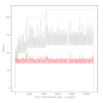
Figure 1.: A trace of the memory used while processing 121 fields (3.6Gb) of an SDSS imaging run on a single 800MHz alpha processor. A total of 165029 objects were detected and charcterised in 5 bands, giving a rate of 13.4ms/object/band for processing from raw CCD frame to reduced catalog. The figure has three lines illustrating memory usage versus time. The lower line is the memory actively in use; the middle dotted line shows the memory in heap, and the top line shows the memory allocated from the system. The difference between the upper two lines is guaranteed to be in 10Mb blocks, all except one of which is completely unused, and can safely be assumed to be swapped out to disk.

2.2. Command Interpreter

We use a heavily enhanced version of TCL 7.4 (actually, of TCLX) as our command language. Much of the work developing this system (known as dervish, né shiva, Sergey et al. 1996) was carried out at FNAL.

In addition to what now appear to be basically cosmetic changes (which we regret), the major enhancements that we made were:

• Memory tracing/defragmentation/debugging

  A common problem with programs that make heavy use of dynamically allocated memory is that the memory acquired from the operating system becomes fragmented, or that the program forgets to free resources. Both of these problems can be resolved by adding a layer above malloc, and we have done so. Figure 1 shows that the total memory used in the steady state by the frames pipeline (see below) is well controlled.

• Support for C datatypes at tcl level.

  We wrote a processor that scans the C include files (‘.h files’) and generated a description of the schema of all the types declared therein. This was originally used to implement a primitive persistent store, but proved more useful in making the C data elements available at the TCL prompt; this greatly increased the power and flexibility of our command language, allowing us to build the command-and-control parts of our pipelines in TCL rather than having to use compiled C. For example, assert {[exprGet $c.calib<$i>->filt<0>] == $f} handleSet $fieldparams.frame<$i>.fullWell<0> $fullWell(0,$f) where a ‘handle’ is an address and a datatype.

• Easy(ish) bindings from C to tcl.

  We implemented a set of library calls that made it possible to bind C commands to TCL in a way that, if not simple, at least required no thought and could be handled by pasting appropriate boiler-plate code.

If we were starting this problem today, we would probably not use TCL (maybe python in its PyRAF [D-05] incarnation?), and we would certainly make greater efforts to use vanilla, up-to-date, versions of our chosen system.

3. Imaging Pipelines

The SDSS has quite a large number of pipelines which must be run in order to fully process the data; we shall not discuss the spectroscopic reductions or the operational and scientific databases.

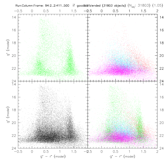
Figure 2.: A $g^{\prime}$ v. $g^{\prime}-r^{\prime}$ colour-magnitude diagram containing 31803 objects from SDSS commissioning data. The bottom two panels show all objects, the top left shows only stars and the top right only galaxies. The disk and halo turnoffs are clearly seen in the stellar diagram. If you are viewing this figure in colour, green points are stars; red points are galaxies classified morphologically as having deVaucouleur-like profiles; cyan points have exponential profiles; and magenta points are unclassified galaxies. In black and white, the bottom two panels are unfortunately indistinguishable

• Astroline

  On the MVE167 processors (running vxWorks) used to archive the raw data on the mountain, we also run a pipeline that processes the pixels before they’re written to disk/tape. We generate star cutouts (‘Postage Stamps’) and column quartiles; this is all that we save from the 22 astrometric CCDs.

• MT Pipeline.

  Process the Photometric Telescope camera data. This consists of a set of staring-mode observations of fields of standard stars, used to define the extinction and photometric zero-points for the 2.5m scans.

• Serial Stamp Collecting (SSC) Pipeline.

  Reorganise the data stream, cut a more complete set of Postage Stamps.

• Astrometric Pipeline.

  Process the centroids of stars from astroline/SSC and generate the astrometric transformations from pixels to $(\alpha,\delta)_{J2000}$ and between bands.

• Postage Stamp Pipeline (PSP).

  Estimate the flat field vectors, bias drift, and sky levels, and characterise the PSF for each field.

• Frames Pipeline.

  Process the full imaging data, producing corrected frames, object catalogues, and atlas images.

• Calibration.

  Take the outputs from MT pipeline and frames, and convert counts to fluxes.

One major gain from splitting responsibilities in this way is that once we get to the frames pipeline, fields (10arcmin$\times$14arcmin patches on the sky) may be processed independently and in any order.

4. Interesting Algorithms

The SDSS imaging piplelines employ a number of novel and even interesting algorithms, which are slowly being written up for publication; for example the image deblender (Lupton 2001). Here we shall only discuss a couple of features connected to handling the point spread function (PSF) and the related problem of star/galaxy separation.

4.1. PSF Estimation

Even in the absence of atmospheric inhomogeneities the SDSS telescope delivers images whose FWHMs vary by up to 15% from one side of a CCD to the other; the worst effects are seen in the chips furthest from the optical axis.

If the seeing were constant in time one might hope to understand these effects ab initio, but when coupled with time-variable seeing the delivered image quality is a complex two-dimensional function and we chose to model it heuristically using a Karhunen-Loève (KL) transform.

Why We Need to Know the PSF

The description of the PSF (as derived in the next subsection) is critical for accurate PSF photometry, i.e. for all faint object photometry — if the PSF varies so does the aperture correction.

We also need to accurately know the PSF in order to be able to separate stars from galaxies; after all, the only valid discriminant that isn’t based on colours or priors is that galaxies don’t look like stars.

A good knowledge of the local PSF is also needed for all studies that measure the shapes of non-stellar objects (e.g. weak lensing studies, Fischer et al. 2000).

KL Expansion of the PSF

The first step is to identify a set of reasonably bright, reasonably isolated stars from our image. We then use these stars to form a KL basis, retaining the first $n$ terms of the expansion:

$$P_{(i)}(u,v)=\sum_{r=1}^{r=n}a^{r}_{(i)}B_{r}(u,v)$$ (1)

where $P_{(i)}$ is the $i^{th}$ PSF star, the $B_{r}$ are the KL basis functions, and $u,v$ are pixel coordinates relative to the origin of the basis functions. In determining the $B_{r}$, the $P_{(i)}$ are normalised to have equal peak value.

Once we know the $B_{r}$ we can write

$$a^{r}_{(i)}\approx\sum_{l=m=0}^{l+m\leq N}b^{r}_{lm}x_{(i)}^{l}y_{(i)}^{m}$$ (2)

where $x,y$ are the coordinates of the centre of the $i^{th}$ star, $N$ determines the highest power of $x$ or $y$ to include in the expansion, and the $b^{r}_{lm}$ are determined by minimising

$$\sum_{i}\left(P_{(i)}(u,v)-\sum_{r=1}^{r=n}a^{r}_{(i)}B_{r}(u,v)\right)^{2};$$ (3)

note that all stars are given equal weight as we are interested in determining the spatial variation of the PSF, and do not want to tailor our fit to the chance positions of bright stars.

Application to SDSS data

For each CCD, in each band, there are typically 15-25 stars in a frame that we can use to determine the PSF; we usually take $n=3$ and $N=2$ (i.e. the PSF spatial variation is quadratic). We need to estimate $n$ KL basis images, and a total of $n(N+1)(N+2)/2$ $b$ coefficients, and at first sight the problem might seem underconstrained. Fortunately we have many pixels in each of the $P_{(i)}$, and thus only the number of spatial terms ($(N+1)(N+2)/2$, i.e. 6 for $N=2$) need be compared with the number of stars available.

In fact, rather than use only the stars from a single frame to determine that frame’s PSF, we include stars from both proceeding and succeeding frames in the fit. This procedure has several advantages: the spatial variation is better constrained at the leading and trailing edges of the frame; the PSF variation is smoother from frame to frame; and the PSF is determined from more stars.

We have found that optimal results are obtained by using a range of $\pm 2$ frames to determine the KL basis functions $B_{r}$ and $\pm 1/2$ frame to follow the spatial variation of the PSF. If we try to use a larger window we find that variation of the $a^{r}$ coefficients is not well described by the polynomials that we have assumed. We have not tried using a different set of expansion functions (e.g. a Fourier series).

4.2. Model Fitting and Star/Galaxy Separation

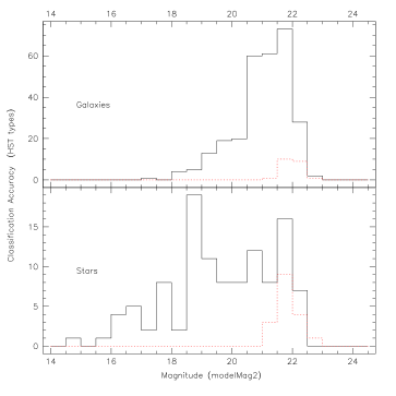
Figure 3.: Star-Galaxy separation in the SDSS. The bottom panel shows object that are classified as stars based on their HST morphology; the top panel shows galaxies. The x-axis is the $r^{\prime}$ model magnitude. The solid line shows the number of objects classified correctly by the SDSS pipeline, the (red) dotted line shows the objects misclassified. It is clear that the performance is quite good, even close to the plate limit at about 22nd.

Figure 4.: The relationship between morphological classification, based on the ratio of the deVaucouleurs and exponential likelihoods. The x-axis is the $u^{\prime}-r^{\prime}$ colour, which divides the galaxies nicely into two classes, presumably early- and late-type (Strateva et al. 2001). The y-axis shows the likelihood ratio (mapped into the range $[0,1]$); above and below the plot are shown the marginal distributions of galaxies which lie outside the pair of dotted lines. The correlation of colour with morhology is clearly seen. Data is from a few square degrees of run 745.

We fit three models to every object, in every band: a PSF, a pure deVaucouleurs profile, and an exponential disk; the galaxy models are convolved with the local PSF (as estimated using the KL expansion of the previous section). This is potentially an expensive operation as it involves a 3-dimensional ($r_{e},a/b,\phi$) non-linear minimisation; each iteration requires the calculation of a 2-d analytical model of a galaxy followed by convolution with the PSF and the calculation of $\chi^{2}$ by summing over many pixels of the image. We make heavy use of pre-calculated tables of models, and pre-extract the radial profile into a series of annuli, each containing 12 30^∘ sectors; in consequence, fitting a single galaxy model in a single band takes of order 1.5ms on an 800MHz alpha.

The primary use of these models is in star/galaxy separation and morphological classification of galaxies. We initially hoped to use the relative likelihoods of the PSF and galaxy fits to separate stars from galaxies, but found that the stellar likelihoods were tiny for bright stars, where the photon noise in the profiles is small, due to the influence of slight errors in modelling the PSF. Instead we found the ratio of the flux in the best-fit galaxy model to that in the PSF to be an excellent discriminant.

Figure 2 shows a colour-magnitude diagram from a small area of SDSS imaging data. The top left panel shows only objects classified as stars; note that most objects with colours of $g^{\prime}-r^{\prime}\approx 0.9$ are preferentially classified as galaxies. The star/galaxy separation is independent of the object’s colours, so this rejection must be a measure of how well the star/galaxy classification is working.

Studies of the performance of the SDSS S/G separation in the Groth strip data (where accurate classification is available from HST imaging) indicate that separation is reliable to at least a $r^{\prime}$ of 21.5 in data that has a $5\sigma$ limit of $r^{\prime}\approx 22$.

The $u^{\prime}-r^{\prime}$ colour of galaxies is a good discriminant of Hubble type (Strateva et al. 2001). Figure 4 shows $u^{\prime}-r^{\prime}$ plotted against what is essentially the likelihood ratio for deVaucouleurs and exponential models shows that the galaxy likelihoods provide clear morphological classification to $r^{\prime}\approx 20$, in data with a PSF $5\sigma$ limit of about 22.5.

5. Conclusions and Software Sociology

As far as he knows, this section represents the views only of the primary author and not of his coauthors. Those of you who know him will have heard these opinions before.

The SDSS has been very challenging technically, scientifically, and managerially. In all categories the software stands out: The hardest technical aspect of building the SDSS was probably the software, although building the mosaic camera wasn’t easy; some of the software was a major scientific challenge; and the software was undoubtedly the hardest part of the project to manage.

Let me expand upon some of these issues. We have found it extremely hard to hire good people to work on astronomical software. There is no career path within the universities for software specialists, despite the fact that there’s no logical distinction between building hard- and soft-ware instruments. Smart and sensible graduate students, desirous of a career in astronomy, simply don’t choose to specialise in the software required to reduce modern observational datasets.

Hiring computer professionals is not the solution to this problem. Besides being (if competent) too expensive for the average astronomical project, they simply don’t possess the skills needed to solve the scientific challenges posed by astronomical data. We need scientists to resolve scientific problems, albeit with support from people whose job it is to know about optimizers, LALR(1) grammars, and good software engineering practices. We also need our software-scientists to be in rich scientific environments, where they can talk with (e.g.) the quasar-scientists about the data analysis that they are carrying out.

If we, as a community, knew how to reuse software from one project on another some of these problems might be alleviated, but I don’t believe that they would go away. The availability of good numerical libraries hasn’t made the development of new cosmological codes stop; the impetus for change comes from the desire to do things better, not just from the not-invented-here syndrome.

I believe that part of the problem is that we, as a community have not yet faced the reality that software is difficult, and that the dynamic range between the really good and the average programmer is as great as that between Lyman Spitzer and the average graduate student. This makes management difficult; imagine trying to get a collaboration of 100 self-opinionated astronomers to agree about the best way to solve a problem, and tell me why this is any easier than running a large modern collaboration involving large amounts of software. I reluctantly believe that we must learn to run large software projects (and all large projects nowadays are large software projects) as benevolent dictatorships — of course with the implicit hope that I shall be the dictator (but not the manager).

Acknowledgments.

The Sloan Digital Sky Survey (SDSS) is a joint project of The University of Chicago, Fermilab, the Institute for Advanced Study, the Japan Participation Group, The Johns Hopkins University, the Max-Planck-Institute for Astronomy, New Mexico State University, Princeton University, the United States Naval Observatory, and the University of Washington. Apache Point Observatory, site of the SDSS telescopes, is operated by the Astrophysical Research Consortium (ARC).

Funding for the project has been provided by the Alfred P. Sloan Foundation, the SDSS member institutions, the National Aeronautics and Space Administration, the National Science Foundation, the U.S. Department of Energy, Monbusho, and the Max Planck Society.

The SDSS Web site is http://www.sdss.org/.

References

Blanton M., et al. The Luminosity Function of Galaxies in SDSS Commissioning Data, 2001, submitted to AJ.

Fan, X. et al. 2000, The Discovery of a Luminous $z=5.80$ Quasar from the Sloan Digital Sky Survey, AJ, 120, 1167.

Fan, X. et al. 2001, High-Redshift Quasars Found in Sloan Digital Sky Survey Commissioning Data IV: The High-Redshift Quasar Luminosity Function, AJ, 121, 54

Fischer, P. et al. 2000, Weak Lensing Measurements of Galaxy Halos with the SDSS I, Commissioning Data, 2000, AJ, 120, 1198

Gunn, J. E. et al. 1988, The Sloan Digital Sky Survey Imaging Camera, AJ, 116, 3040

Ivezić Z., et al. 2000 Candidate RR Lyrae Stars Found in Sloan Digital Sky Survey Commissioning Data, AJ, 120, 963.

Leggett, S.K. et al. 2000, The Missing Link: Early Methane (“T”) Dwarfs in the Sloan Digital Sky Survey ApJ, 536, L35

Lupton, R. H. et al. 2001, SDSS Image Processing I: The Deblender AJ, submitted

Sergey G., et al. in ASP Conf. Ser., Vol. 101, Astronomical Data Analysis Software and Systems V, ed. G. H. Jacoby & J. Barnes (San Francisco: ASP).

Strateva I., et al. 2001, in Preparation.

York, D. G. et al. 2000, The Sloan Digital Sky Survey: Technical Summary, AJ, 120, 1579