A photometricity and extinction monitor at the Apache Point Observatory

Abstract

An unsupervised software “robot” that automatically and robustly reduces and analyzes CCD observations of photometric standard stars is described. The robot measures extinction coefficients and other photometric parameters in real time and, more carefully, on the next day. It also reduces and analyzes data from an all-sky $10~{}\mathrm{\mu m}$ camera to detect clouds; photometric data taken during cloudy periods are automatically rejected. The robot reports its findings back to observers and data analysts via the World-Wide Web. It can be used to assess photometricity, and to build data on site conditions. The robot’s automated and uniform site monitoring represents a minimum standard for any observing site with queue scheduling, a public data archive, or likely participation in any future National Virtual Observatory.

1. Introduction

More and more, astronomical research is being performed remotely, in the sense that the observer, or perhaps more properly “data analyst”, is now often not present at the place or time at which observations are taken. The increase in remoteness has several causes. One is that for many observatories, telecommunication is easier than travel, especially if telescope allocations are of short durations. Another is that several new telescopes are using or plan to use queue-scheduling (eg, contributions to Boroson et al (1996); and Boroson et al (1998), Garzon & Rozas (1998), Tilanus (2000), Massey et al (2000)), for which observer travel is essentially impossible. Some new ground-based telescopes are partially or completely robotic (eg, contributions to Filippenko (1992), contributions to Adelman et al (1992); and Baruch & da Luz Vieira (1993), Akerlof et al (1999), Castro-Tirado et al (1999), Strassmeier et al (2000), Querci & Querci (2000)). Possibly the most important reason for the increase in remote observing is that many observatories, many large surveys, and some independent organizations are creating huge public data archives which allow analyses by anyone at any time (eg, contributions to Mehringer et al (1999) and Manset et al (2000)). There has been community discussion of a “National Virtual Observatory” which might be a superset of these archives and surveys (eg, contributions to Brunner et al (2001)).

Remote observing and archival data analysis bring huge economic and scientific benefits to astronomy, but with the significant cost that the observer does not have direct access to observing conditions at the site. Most remote observatories and data archives keep logs written by telescope operators, but these logs are notoriously non-uniform in their attention to detail and use of terminology. All sites that plan to host remote observers or maintain public data archives must have repeatable, quantitative, astronomically relevant site monitoring.

For these reasons, among others (involving photometric calibration and direction of survey operations) the Sloan Digital Sky Survey (SDSS; York et al (2000)), which is constructing a public database of $10^{4}~{}\mathrm{deg}^{2}$ of five-bandpass optical imaging and $10^{6}$ optical spectra, employs several pieces of hardware for monitoring of the Apache Point Observatory site, including a $10$-$\mathrm{\mu m}$ cloud-camera scanning the whole sky (Hull et al (1994)), a single-star atmospheric seeing monitor, a low-altitude dust particle counter, a basic weather station, and a 0.5-m telescope making photometric measurements of a large set of standard stars. This paper is about a fully automated software “robot” that reduces the raw 0.5-m telescope data, locates and measures standard stars, and determines atmospheric extinction in near-real time, reporting its findings back to telescope and survey operators via the World-Wide Web (WWW). This paper describes the software robot, rather than the hardware, which will be the subject of a separate paper (Uomoto et al in preparation).

Although the robot is somewhat specialized to work with the hardware and data available at the Apache Point Observatory, it could be generalized easily for different hardware. We are presenting it here because it might serve as a prototype for site monitors that ought to be part of any functional remote observing site and of the National Virtual Observatory.

2. Telescope and detector

The primary telescope used in this study is the Photometric Telescope (PT) of the SDSS, located at the Apache Point Observatory (APO) in New Mexico, at latitude 32 46 49.30 N, longitude 105 49 13.50 W, and elevation 2788 m. The PT has a 20-in primary mirror and is outfitted with a $2048\times 2048$ pixel CCD with 1.16 arcsec pixels, making for a $40\times 40~{}\mathrm{arcmin^{2}}$ field of view. The telescope and CCD will be described in more detail elsewhere (Uomoto et al in preparation).

The telescope takes images through five bandpasses, $u^{\prime}$, $g^{\prime}$, $r^{\prime}$, $i^{\prime}$, and $z^{\prime}$, chosen to be close to those in the SDSS 2.5-m imaging camera. Filter wavelengths are given in Table 1. The magnitude system here is based on an approximation to an AB system (Oke & Gunn (1983), Fukugita et al (1996)), again because that was the choice for the SDSS imaging. The photometric system will be described in more detail elsewhere (Smith et al in preparation). Nothing about the function of the robot is tied to this photometric system; any system can be used provided that there is a well-calibrated network of standard stars.

3. Observing strategy

Site monitoring and measurement of atmospheric extinction is only one part of the function of the Photometric Telescope (PT). The PT is being simultaneously used to take data on a very large number of “secondary patches” that will provide calibration information for the SDSS imaging. For this reason, the PT spends only about one third of its time monitoring standard stars. Its site monitoring and atmospheric extinction measuring functions could be improved significantly, in signal-to-noise and time resolution, if the PT were dedicated to these tasks.

The observing plan for the night is generated automatically by a field “autopicker” which chooses standard star fields on the basis of (a) observability, (b) airmass coverage, (c) intrinsic stellar color coverage, and (d) number of calibrated stars per standard field. Because the observing is very regular, with $u^{\prime}$, $g^{\prime}$, $r^{\prime}$, $i^{\prime}$, and $z^{\prime}$ images taken (in that order) of each field, it has been almost entirely automated. The only significant variation in observing from standard field to standard field is that different fields are imaged for different exposure times to avoid saturation.

The raw data from the telescope is in the form of images in the Flexible Image Transport System format (FITS; Wells et al (1981)). The raw image headers contain the filter (bandpass) used, the exposure time, the date and UT at which the exposure was taken, the approximate pointing of the telescope in RA and Dec, and the type of exposure (eg, bias, flat, standard-star field, or secondary patch). The robot makes use of much of this information, as described below.

4. Obtaining and manipulating the data

In principle, the photometricity monitoring software could run on the data-acquisition computer. However, in the interest of limiting stress on the real-time systems, the photometricity robot runs on a separate machine, obtaining its data by periodic executions of the UNIX rsync software. The rsync software performs file transfer across a network, using a remote-update protocol (based on file checksums) to ensure that it only transfers updated or new files, without duplicating effort. The output of rsync can be set to include a list of the files which were updated. This output is passed (via scripts written in the UNIX shell language bash) to a set of software tools written in the data-analysis language IDL.

Virtually all of the image processing, data analysis, fitting, and feedback to the observer is executed with IDL programs in bash wrappers. This combination of software has proven to be very stable and robust over many months of continuous operation. In addition, data reduction code written in IDL is easy to develop and read. Our only significant reservation is that IDL is a commercial product which is not open-source. We have responded to this lack of transparency by writing as much as possible of the robot’s function in terms of very low-level IDL primitives, which could be re-written straightforwardly in any other data-analysis language if we lost confidence in or lost access to IDL. We have not found the lack of transparency to be limiting for any of the functionality described in this paper.

5. Correcting the images

Each raw image is bias-subtracted and flattened, using biases and flat-field information archived from the most recent photometric night. How the bias and flat images are computed from a night’s data is described in Section 11, along with the conditions on which a night is declared photometric.

Because the CCD is thinned for sensitivity in the $u$ bandpass, it exhibits interference fringing in the $i^{\prime}$ and $z^{\prime}$ bandpasses. The fringing pattern is very stable during a night and from night to night. The fringing is modeled as an additive distortion; it is removed by subtracting a “fringe image” scaled by the DC sky level. How the fringe image is computed is described in Section 11. The DC sky level is estimated by taking a mean of all pixels in the image, but with iterated “sigma-clipping” in which the rms pixel value is computed, 3.5-sigma outlier pixels are discarded, and the mean and rms are re-estimated. This process is iterated to convergence. The fringing correction is demonstrated in Figure 1. Although in principle the fringing pattern may depend on the temperature or humidity of the night sky, it does not appear to vary significantly within a night, or even night-to-night. Perhaps surprisingly, the fringing pattern appears fixed and its amplitude scales linearly with the DC level of the sky.

For each corrected PT image, a mask of bad pixels is retained. The mask is the union of all pixels saturated in the raw images along with all pixels which are marked as anomalous in the bias image, flat image, or (for the $i^{\prime}$ and $z^{\prime}$ bandpasses) fringe image. How pixels are marked as anomalous in the bias, flat, and fringe is described in Section 11.

The individual bias-subtracted, flattened and (for the $i^{\prime}$ and $z^{\prime}$ bandpasses) fringe-corrected image will, from here on, be referred to as the “corrected frames”. The corrected frames are stored and saved by the robot in FITS format.

6. Astrometry and source identification

Hardware pointing precision is not adequate for individual source identifications. The software robot determines the precise astrometry itself, by comparison with the USNO-SA2.0 astrometric catalog (Monet et al (1998)). This catalog contains $5\times 10^{7}$ astrometric stars over most of the sky; there are typically a few $10^{2}$ catalog stars inside a PT image.

In brief, the astrometric solution for each image is found as follows: A sub-catalog is created from all astrometric stars within 30 arcmin of the field center (as reported by the hardware in the raw image header). An implementation of the DAOPHOT software (Stetson (1987), Stetson (1992)) in IDL (by private communication from W. Landsman) is used to locate all bright point sources in the corrected frame (DAOPHOT is used for object-finding only, not photometry). Each set of stars is treated as a set of delta-functions on the two-dimensional plane of the sky, and the cross-correlation image is constructed. If there is a statistically significant cluster of points in the cross-correlation image, it is treated as the offset between the two images. Corresponding positions in the two sets of stars (from the corrected frame and from the astrometric catalog) are identified, and the offset, rotation, and non-linear radial distortion in the corrected frame are all fit, with iterative improvement of the correspondence between the two sets of stars. The precise astrometric information is stored in the FITS header of each corrected frame in GSSS format (this format is not standard FITS but is used by the HST Guide Star Survey; cf. Russell et al (1990), Calabretta & Greisen (2000)). Our algorithm is much faster, albeit less general, than previous algorithms (eg, Valdes et al (1995)).

Essentially all exposures of more than a few seconds in the $g^{\prime}$, $r^{\prime}$ and $i^{\prime}$ bandpasses obtain correct astrometric solutions by this procedure. Some short $u^{\prime}$ and $z^{\prime}$ exposures do not, and are picked up on a second pass using a mini-catalog constructed from stars detected in the $g^{\prime}$ and $r^{\prime}$ exposures of the same field. On most nights, all exposures in all bands obtain correct astrometric solutions.

The algorithm and its implementation will be discussed in more detail in a separate paper, as it has applications in astronomy that go beyond this project.

7. Photometry

The robot measures and performs photometric fits with the stars in the SDSS catalog of photometric standards (Smith et al in preparation). This catalog includes stars in the range $6<r<15$ mag, calibrated with the USNO 40-inch Ritchey-Chrétien Telescope. Several of the standard-star fields used in this catalog are well-studied fields (Landolt (1992)) containing multiple standard stars spanning a range of magnitude and color.

The photometric catalog is searched for photometric standard stars inside the boundaries of each corrected frame with precise astrometric header information. If any stars are found in the photometric catalog, aperture photometry is performed on the point source found at the astrometric location of each photometric standard star. The centers of the photometric apertures are tweaked with a centroiding procedure which allows for small ($\lesssim 1$ arcsec) inaccuracies in absolute astrometry. The aperture photometry is performed in focal-plane apertures of radii 4.63, 7.43, and 11.42 arcsec. The sky value is measured by taking the mean of the pixel values in an annulus of inner radius 28.20 and outer radius 44.21 arcsec, with iterated outlier rejection at 3 sigma. All of these angular radii are chosen to match those used by the SDSS PHOTO software (Lupton et al (2001), Lupton et al in preparation).

In what follows, the 7.43-arcsec-radius aperture photometry is used. This aperture was chosen from among the three for showing, on nights of typical seeing, the lowest-scatter photometric solutions. This is because, in practice, the 7.43-arcsec-radius aperture is roughly the correct trade-off between individual measurement signal-to-noise (which favors small apertures) and insensitivity to spatial or temporal variations in the point-spread function (which favors large). The PT shows significant, repeatable, systematic distortions of the point-spread function across the field of view; a more sophisticated robot would model and correct these distortions; for our purposes it is sufficient to simply choose the relatively large 7.43-arcsec-radius aperture.

Each photometric measurement is corrected for its location in the field of view of the PT. There are two corrections. The first is an illumination correction derived from the radial distortion of the field as found in the precise astrometric solution (Section 6). The illumination correction is designed to account for the fact that photometrically we are interested in fluxes, but the flatfield is measured with the sky; ie, the flatfield is made to correct pixels to a constant surface-brightness sensitivity rather than a constant flux sensitivity. Because of optical distortions, pixels near the edge of the CCD see a different solid angle than pixels near the center. Empirically, the dominant field distortion appears radial, so no attempt has been made to correct for illumination variation from arbitrary distortions. The illumination correction reaches a maximum of $\sim 0.02$ mag at the field edges and $\sim 0.04$ mag at the field corners.

The second correction is related to the fringing in the $i^{\prime}$ and $z^{\prime}$ bandpasses. The CCD is thinned, but not precisely uniformly; the dominant thinning gradients are radial. Because of reflections internal to the CCD, gradients in CCD thickness lead to gradients in the fraction of point-source light scattered out of the seeing core and into the sky level. Since the flat-field is computed on the basis of sky level, these gradients are seen as residuals in photometry. Radial photometry corrections for the $i^{\prime}$ and $z^{\prime}$ bandpasses were found by performing empirical fits to photometry residuals; they are applied to the $i^{\prime}$ and $z^{\prime}$ bandpass photometry. These “thinning” corrections reach a maximum of $[\Delta i^{\prime},\Delta z^{\prime}]\sim[0.02,0.05]$ mag at the field edges and $\sim[0.03,0.07]$ mag at the field corners.

8. Cloud detection and data veto

The “prototype cloud camera” (Hull et al (1994)) operating at APO utilizes a single-pixel cooled $10~{}\mathrm{\mu m}$ detector and scanning mirrors. The sky is scanned by two flat mirrors driven by stepper motors, followed by an off-axis hyperbolic mirror that images the sky onto a single channel HgCdTe photoconductive detector. The detector samples 300 times per scan, 300 scans per image, yielding an image with $300\times 300$ pixels covering a $135\times 135~{}\mathrm{deg^{2}}$ field with the $0.9$ deg beam. Some typical images are shown in Figure 2. An image is completed in approximately 5 min. This is somewhat slow for real-time monitoring, but perfectly adequate for our purposes. This design was prefered over a solid state array for reasons of price, stability, and field of view. A disadvantage is the maintenance required by moving parts, but this has not been a serious drawback.

Experimentation showed that a simple and adequate method for detecting cloud cover is to compute the rms value of the sky within 45 deg of zenith in each frame. This seems to be a simple and robust method, and it fails only in the case of unnaturally uniform cloud cover (this has never occurred). When the cloud-camera rms exceeds a predefined threshold for a period of time, that period is declared bad, and the data taken during that interval are ignored for photometric parameter fitting. The bad interval is padded by 20 min on each end, so that even a single cloud appearing in one frame requires discarding at least 40 min of data. This is conservative, but it is more robust to set the cloud threshold high and reject significant time intervals than to make the threshold extremely low.

9. Photometric solution

Every time the PT completes a set of $u^{\prime},g^{\prime},r^{\prime},i^{\prime},z^{\prime}$ exposures in a field, the robot compiles all the measurements made of photometric standard stars in that night and fits photometric parameters to all data not declared bad by the cloud-camera veto (Section 8). The photometric equations used for the five bandpasses are

$$u^{\prime}_{\mathrm{inst}} = u_{\mathrm{USNO}}+a_{u}+b_{u}\,(u-g)_{\mathrm{USNO}}+k_{u}\,X$$

$$+c_{u}\,[X-X_{0}]\,[(u-g)_{\mathrm{USNO}}-(u-g)_{0}]$$

$$+\dot{a}_{u}\,[t-t_{0}]]$$

$$g^{\prime}_{\mathrm{inst}} = g_{\mathrm{USNO}}+a_{g}+b_{g}\,(g-r)_{\mathrm{USNO}}+k_{g}\,X$$

$$+c_{g}\,[X-X_{0}]\,[(g-r)_{\mathrm{USNO}}-(g-r)_{0}]$$

$$+\dot{a}_{g}\,[t-t_{0}]]$$

$$r^{\prime}_{\mathrm{inst}} = r_{\mathrm{USNO}}+a_{r}+b_{r}\,(r-i)_{\mathrm{USNO}}+k_{r}\,X$$

$$+c_{r}\,[X-X_{0}]\,[(r-i)_{\mathrm{USNO}}-(r-i)_{0}]$$

$$+\dot{a}_{r}\,[t-t_{0}]]$$

$$i^{\prime}_{\mathrm{inst}} = i_{\mathrm{USNO}}+a_{i}+b_{i}\,(i-z)_{\mathrm{USNO}}+k_{i}\,X$$

$$+c_{i}\,[X-X_{0}]\,[(i-z)_{\mathrm{USNO}}-(i-z)_{0}]$$

$$+\dot{a}_{i}\,[t-t_{0}]]$$

$$z^{\prime}_{\mathrm{inst}} = z_{\mathrm{USNO}}+a_{z}+b_{z}\,(i-z)_{\mathrm{USNO}}+k_{z}\,X$$ (1)

$$+c_{z}\,[X-X_{0}]\,[(i-z)_{\mathrm{USNO}}-(i-z)_{0}]$$

$$+\dot{a}_{z}\,[t-t_{0}]]$$

where the $m_{\mathrm{inst}}$ symbolize instrumental magnitudes defined by

$$m_{\mathrm{inst}}\equiv-2.5\,\log_{10}\left(\frac{DN}{t_{\mathrm{exp}}}\right)$$ (2)

with $DN$ the flux in raw counts in the corrected frame and $t_{\mathrm{exp}}$ the exposure time; the $m_{\mathrm{USNO}}$ symbolize the magnitudes in the photometric standard-star catalog; $X$ symbolizes airmass; $t$ symbolizes time (UT); $X_{0}$, $t_{0}$, and the colors $(u-g)_{0}$, etc, symbolize fiducial airmass, time, and colors (arbitrarily chosen but close to mean values); and the $a$, $b$, $k$, $c$, and $\dot{a}$ parameters are, in principle, free to vary. The system sensitivities are the $a_{i}$; the tiny differences in photometric systems between the USNO 40-inch and PT bandpasses are captured by the color coefficients $b_{i}$; the atmospheric extinction coefficients are the $k_{i}$; atmospheric extinction is a weak function of intrinsic stellar color parameterized by the $c_{i}$; and the $\dot{a}_{i}$ parameterize any small time evolution of the system during the night.

The above photometric equations are not strictly correct for an AB system, because in the AB system, there is no guarantee that the colors of standard stars through two slightly different filter systems will agree at zero color; this agreement is assumed by the above equations. In an empirical system, such as the Vega-relative magnitude system, a certain star, such as Vega (and stars like it) have zero color in all colors of all filter systems. The AB system is based on a hypothetical source with $f_{\nu}=\mathrm{const}$; there is no guarantee that a source with zero color in one filter system will have zero color in any other. The offsets must be computed theoretically, using models of CCD efficiencies, mirror reflectivities, atmospheric absorption spectra, and intrinsic stellar spectral energy distributions. We have ignored this (subtle) point, since it only leads to offsets in the sensitivity parameters $a_{i}$ and does not affect photometricity or atmospheric extinction assessments.

In practice, the $c$ parameters are always fixed at theoretically derived values

$$c_{u} = -0.021~{}\mathrm{mag\,mag^{-1}\,airmass^{-1}}$$

$$c_{g} = -0.016$$

$$c_{r} = -0.004$$

$$c_{i} = +0.006$$

$$c_{z} = +0.003$$ (3)

The $\dot{a}$ parameters are only allowed to be non-zero in the next-day analysis (Section 11). Because the design specification on the PT did not require correct airmass values in raw image headers, the airmass values are computed on the fly from the RA, Dec, UT, and location of the Observatory (eg, Smart (1977)). The reference airmass and colors are chosen to be roughly the mean on a typical night of observing, or

$$X_{0}=1.30~{}\mathrm{airmass}$$ (4)

$$(u-g)_{0} = +1.42~{}\mathrm{mag}$$

$$(g-r)_{0} = +1.11$$

$$(r-i)_{0} = +0.48$$

$$(i-z)_{0} = +0.35$$ (5)

(in the AB system). In the next-day analysis, the reference time $t_{0}$ is set to be the mean UT of the observations.

In principle the color coefficients $b_{i}$ could be determined globally and fixed once and for all. However, the PT filters have been shown to have some variation with time and with humidity (they are kept in a low-humidity environment with some variability), so the robot fits them independently every night. Freedom of the $b_{i}$ is allowed not because it is demanded by the data, but rather because measurements of the $b_{i}$ over time are an important part of data and telescope quality monitoring. Typical color coefficient values (which measure differences between the USNO 40-inch telescope and PT bandpasses) are

$$b_{u} = +0.048~{}\mathrm{mag\,mag^{-1}}$$

$$b_{g} = -0.004$$

$$b_{r} = -0.028$$

$$b_{i} = -0.053$$

$$b_{z} = -0.031$$ (6)

Quite a bit of experimentation went into the photometric equations. Inclusion of theoretically determined $c$ parameters minutely improves the fit, but on a typical night there are not enough data to determine the $c$ parameters empirically; the $c_{i}$ are held fixed. Terms proportional to products of time and airmass, again, are not well constrained from a single night’s data; they are not included in the fit. To each bandpass a color is assigned; the choices have been made to use the most well-behaved “adjacent” colors. (The $(u-g)$ color is not used for the $g$ equation because the boundary between $u$ and $g$ is, by design, on the 4000 Å break, making color transformations extremely sensitive to the precise properties of the filter curves.)

In the real-time analyses, the $a$, $b$, and $k$ parameters (15 total) are fit to the counts from the aperture photometry (and USNO magnitudes, times, airmasses, etc) with a linear least-square fitting routine, which iteratively removes 3.0-sigma outliers and repeats its fit. A typical night at APO shows extinction coefficients

$$k_{u} = 0.52~{}\mathrm{mag\,airmass^{-1}}$$

$$k_{g} = 0.19$$

$$k_{r} = 0.12$$

$$k_{i} = 0.08$$

$$k_{z} = 0.06$$ (7)

with factor of $\sim 1.5$ variations from night to night.

All photometric measurements are weighted equally in these fits, because the error budget appears to be dominated by systematic errors in the USNO catalog and sky subtraction; the primary errors are not from photon statistics. As observing continues and iterative improvement to the USNO catalog is made, we will be able to use a more sophisticated weighting model; we don’t expect such improvements to significantly change the values of our best-fit photometric parameters.

On a typical night, 5-band measurements are made of 20 to 50 standard stars in 10 to 15 standard-star fields.

10. Real-time observer feedback

Every ten minutes during the night (from 18:00 to 07:00, local time), the robot builds a WWW page in Hypertext Markup Language (HTML) reporting on its most up-to-date photometric solution. The WWW page shows the best-fit $a$, $b$ and $k$ parameter values, plots of residuals around the best photometric solution in the five bandpasses, and root-mean-squares (rms) of the residuals in the five bandpasses. Parameters or rms values grossly out-of-spec are flagged in red. This feedback allows the observers to make real-time decisions about photometricity, and confirm expectations based on visual impressions of and 10-$\mathrm{\mu m}$ camera data on atmospheric conditions. The WWW page also includes an excerpt from the observers’ manually entered log file. This allows those monitoring the site remotely to compare the observers’ and robot’s photometricity judgements. Figures 3 and 4 show examples of the photometricity output on the WWW page on two typical nights.

The WWW page also shows data from the APO weather, dust, and cloud monitors for comparison by the observers, as do Figures 3 and 4.

Since WWW pages in HTML are simply text files, they are trivially output by IDL. The figures on the WWW pages are output by IDL as PostScript files and then converted to a (crudely) antialiased pixel image with the UNIX command ghostscript and the UNIX pbmplus package.

11. Next-day analysis and feedback

At 07:00 (local time) each day, the robot begins its “next-day” analysis, in which all the data from the entire night (just ended) are re-reduced and final decisions are made about photometricity and data acceptability.

Bias frames taken during the night are identified by header keywords. The bias frames are averaged, with iterated outlier rejection, to make a bias image. Any pixels with values more than 10-sigma deviant from the mean pixel value in the bias image are flagged as bad in a bias mask image.

Dome and sky flat frames are identified by header keywords. These raw images are bias-subtracted using the bias image. Each bias-subtracted image is divided by its own mean, which is estimated with iterated outlier rejection. The bias-subtracted and mean-divided flat frames are averaged together, again with iterated outlier rejection, to make five flat images, one for each bandpass. Any pixels with values more than 10-sigma deviant from the mean are flagged as bad in flat mask images.

The $i$ and $z$-bandpass images are affected by an interference fringing pattern, which is modeled as an additive distortion. Any $i$ or $z$-bandpass image taken during the night with exposure time $t_{\mathrm{exp}}>100$ s is identified. These long-exposure frames are bias-subtracted and divided by the flat. Each is divided by its own mean, again estimated with iterated outlier rejection. These mean-divided frames are averaged together, again with iterated outlier rejection to make two fringe correction images, in the $i^{\prime}$ and $z^{\prime}$ bandpasses. Again, 10-sigma outlier pixels are flagged as bad in fringe mask images.

Constant bias, flat and fringe images are used for the entire night; there is no evidence with this system that there is time evolution in any of these.

All the raw images from the night are bias-subtracted and flattened with these new same-night bias and flat images. The $i^{\prime}$ and $z^{\prime}$-bandpass images are also fringe-corrected. Thus a new set of corrected frames is constructed for that night. The real-time astrometry solutions are re-used in these new corrected frames. All photometry is re-measured in the new corrected frames.

A final photometric parameter fit is performed with the new measurements, again with removal of data declared bad by the cloud-camera veto, and with iterated outlier rejection. The only difference is that the time evolution $\dot{a}$ terms are allowed to be non-zero.

Because we expect non-zero $\dot{a}$ terms to be caused by changing atmospheric conditions, we experimented with allowing time evolution in the extinction coefficients (eg, $\dot{k}$ terms). Unfortunately, such terms involve non-linear combinations of input data (time times airmass) and can only be added without introducing biases if there are *also* $\dot{a}$ terms; ie, it is wrong in principle to include $\dot{k}$ terms without also adding $\dot{a}$ terms, especially in the face of iterated outlier rejection. We found that adding both $\dot{a}$ and $\dot{k}$ terms did not improve our fits relative to simply adding $\dot{a}$ terms, so we have not included $\dot{k}$ terms. With more frequent standard-star sampling, the time resolution of the system would be improved and $\dot{k}$ terms would, presumably, improve the fits.

The entire next-day re-analysis takes between three and six hours, depending on the amount of data. Much of the computer time is spent swapping processes in and out of virtual memory; with more efficient code or larger RAM the re-analysis time could be reduced to under two hours. The re-analysis would take one to two hours longer if it were necessary to repeat the astrometric solutions found in the real-time analysis.

At the end of the re-analysis, the robot constructs a “final” WWW page, similar to the real-time feedback WWW page, but with the final photometric solution and residuals. Parameters grossly out-of-spec are shown in red. Also, the robot sends an email to a SDSS email archive and exploder, summarizing the final parameter values and rms residuals in the five bands.

For the robot’s purposes, a night is declared “photometric” if the rms residual around the photometric solution (after iterated outlier rejection at the 3-sigma level) in the $[u^{\prime},g^{\prime},r^{\prime},i^{\prime},z^{\prime}]$ bandpasses is less than $[0.03,0.02,0.02,0.02,0.03]$ mag. If the night is declared photometric, then the bias, flat, and fringe images and their associated pixel masks are declared “current,” to be used for the real-time analysis of the following nights.

Figure 5 shows the final fits for an example night, with and without the inclusion of the veto of data taken during cloudy periods. This is a night which would have been declared marginally non-photometric without the cloud-camera veto, but became photometric when the cloudy periods were removed.

12. Archiving

All raw PT data are saved in a tape archive at Fermi National Accelerator Laboratory (FNAL). In addition, about one year’s worth of the most recent data are archived on the robot machine itself, on a pair of large disk drives. The photometric parameters from each photometric night are kept in a FITS binary table (Cotton et al (1995)), labeled by observation date. These parameter files are mirrored in directories at FNAL and elsewhere (DWH’s laptop, for example). Because the astrometric solutions are somewhat time-consuming, the astrometric headers for all the corrected frames are also saved on disk on the robot machine and mirrored, along with each night’s bias, flat, and fringe images. Because the astrometric header information is all saved, along with the bias, flat, and fringe images, the corrected frames can be reconstructed trivially and quickly from the raw data.

13. Scientific output

The archived output data from the photometricity monitor robot is not just useful for verifying and analyzing contemporaneous data from the Observatory. It contains a wealth of scientific data useful for analyzing long-term behavior and pathologies of the site, the hardware, and the standard star catalog. Many of these analyses will be performed and presented elsewhere, as the site monitoring data builds up.

As an example, Figure 6 shows the atmospheric extinction coefficients $[k_{u},k_{g},k_{r}]$ plotted against one another, for most of the photometric nights in roughly one-third of a year. This Figure shows the variability in the extinction coefficients, as well as their covariance. If the variability in the extinction is due to varying optical depth of a single component of absorbing material, the covariances should fall along the grey diagonal lines (ie, $k_{u}\propto k_{g}\propto k_{r}$). Although the $k_{g}$ vs $k_{r}$ plot is consistent with this assumption, the $k_{u}$ vs $k_{r}$ plot appears not to be. Perhaps not surprisingly, atmospheric extinction must be caused by multiple atmospheric components. It is at least slightly surprising to us that the variability in $u$-bandpass extinction is smaller than would be predicted from a one-component assumption and the variability in the $r$-bandpass extinction.

14. Comments

The success of this ongoing project shows that robust, hands-off, real-time and next-day photometricity assessment and atmospheric extinction measurement is possible. There is much lore about photometricity, site variability, and precise measurement in astronomy. Most of this lore can be given an empirical basis with a simple system like the one described in this paper.

It is worth emphasizing that the observing hardware used by the robot is not dedicated to the robot’s site monitoring tasks. The PT is being used to calibrate SDSS data; it only spends about one third of its time taking the observations of catalogued standards which are used for photometricity and extinction measurements. This shows that a robot of this type could, with straightforward (if not trivial) adjustment, be made to “piggyback” on almost any observational program, provided that some fraction of the data is multi-band imaging of photometric standard stars. The robot does not rely on the images having accurate astrometric header information, or accurate text descriptions or log entries; it finds standard stars in a robust, hands-off manner. Many observatories could install a robot of this type with no hardware cost whatsoever! A site with no appropriate imaging program on which the robot could “piggyback” could install a small telescope with a good robotic control system, a CCD and filter-wheel, and the robot software described here, at fairly low cost. The telescope need only be large enough to obtain good photometric measurements of some appropriate set of standard stars. All of the costs associated with such a system are going down as small, robotic telescopes are becoming more common (eg, Akerlof et al (1999), Strassmeier et al (2000), Querci & Querci (2000)).

The robot works adequately without input from the $10~{}\mathrm{\mu m}$ cloud camera, as long as data are not taken during cloudy periods, or as long as the observers can mark, in some way accessible to the robot, cloudy data. On the other hand, $10~{}\mathrm{\mu m}$ pixel array cameras, with no moving parts (unlike the prototype camera working at APO) are now extremely inexpensive and would be easy to install and use at any observatory.

The robot system was developed and implemented in a period of about nine months. It has been a very robust tool for the SDSS observers. The rapid development and robust operation can be ascribed to a number of factors: The robot design philosophy has always been to make every aspect of the robot’s operation as straightforward as possible. We have only added sophistication to the robot’s behavior as it has been demanded by the data. The IDL data analysis language has primitives useful for astronomy and it operates on a wide range of platforms and operating systems. Perhaps above all, the PT is a stable, robust telescope (Uomoto et al in preparation).

Without objective, well-understood site monitoring like that provided by this simple robot, analyses of archived and queue-observing data will always be subject to some suspicion. At APO, the visual monitor robot has been a very inexpensive and effective tool for building confidence in observer decisions and for providing feedback to data analysis. With this robot operating, APO has better monitoring of site conditions and data quality than most existing or even planned observatories.

Table 1Approximate PT bandpass information

		$u^{\prime}$	$g^{\prime}$	$r^{\prime}$	$i^{\prime}$	$z^{\prime}$
central wavelength	(Å)	3540	4770	6230	7620	9130
full-width at half-maximum	(Å)	570	1390	1370	1530	950

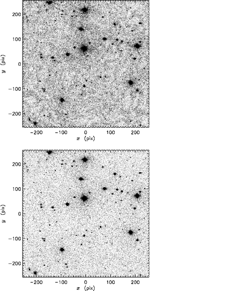
Figure 1.— A $512\times 512~{}\mathrm{pix^{2}}$ ($594\times 594~{}\mathrm{arcsec^{2}}$) section of a bias-subtracted and flat-fielded $z^{\prime}$-bandpass image from the PT, (top) before, and (bottom) after the fringing correction. The two images are stretched identically; in the (top) image, the fringing is roughly 10 percent of the background level, peak-to-peak.

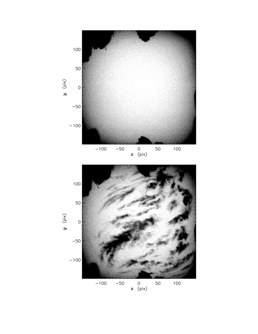
Figure 2.— Two example cloud-camera images, taken (top) at 05:24 UT on MJD 51997, and (bottom) at 05:45 UT on MJD 51997. The images are displayed at the same stretch and are negatives (bright areas appear dark). The dark silhouettes around the edge are buildings and trees near the camera; the APO 3.5-m Telescope is visible in the upper left-hand corner.

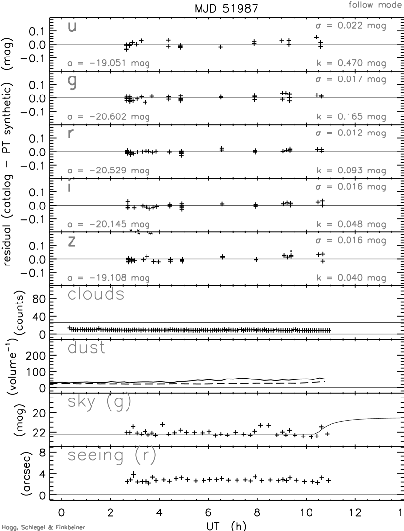
Figure 3.— The real-time WWW output created at 11:00 UT on MJD 51987. This was one of the best nights of the year at APO.

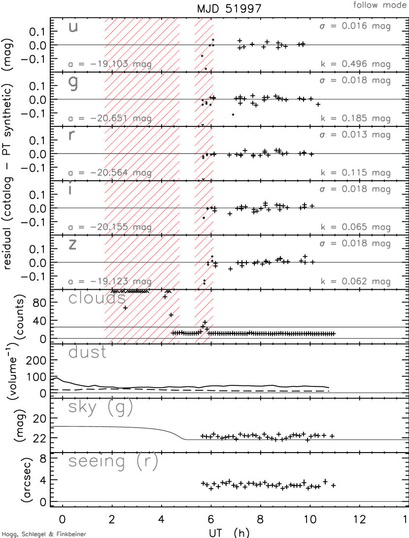
Figure 4.— The real-time WWW output created at 11:00 UT on MJD 51997. The red hatched areas are time intervals vetoed by the cloud-camera analysis. Rejected points are shown with smaller symbols.

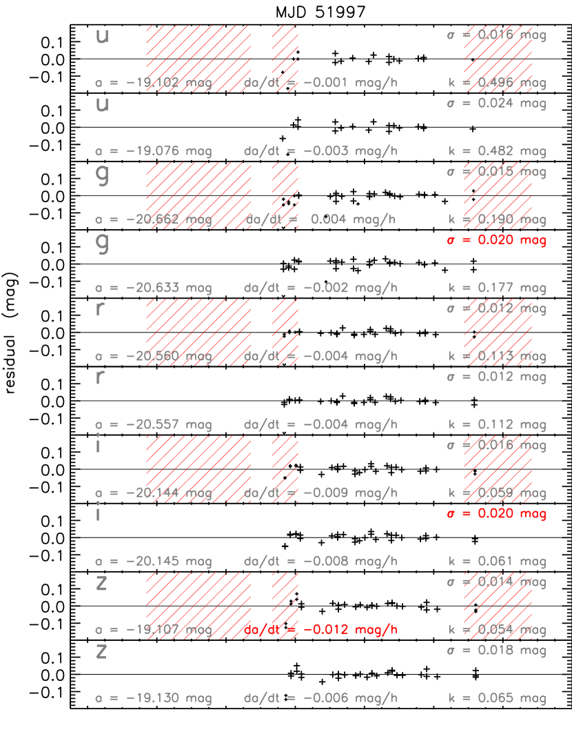
Figure 5.— A comparison of final fits (ie, including $\dot{a}$ terms) in the five bands, for MJD 51997, with and without the data vetoing by cloud-camera. The panels with the red cross-hatching have had data taken during cloudy periods removed from the fit. In most bands, the fit is improved when cloudy data are removed.

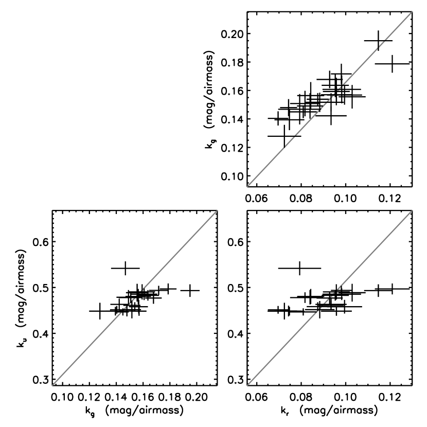
Figure 6.— Atmospheric extinction coefficients $[k_{u},k_{g},k_{r}]$ in the $[u^{\prime},g^{\prime},r^{\prime}]$ bandpasses, for most photometric nights between MJD 51840 and 51970, plotted against one another. The grey lines show the relationship ($k_{u}\propto k_{g}\propto k_{r}$) expected if atmospheric extinction is due to a single atmospheric component.

References

- Adelman et al (1992) Adelman, S. J., Dukes, R. J., & Adelman, C. J. editors 1992, ASP Conf. Ser. 28: Automated Telescopes for Photometry and Imaging
- Akerlof et al (1999) Akerlof, C. et al 1999, Nature, 398, 400
- Baruch & da Luz Vieira (1993) Baruch, J. E. & da Luz Vieira, J. 1993, Proc. SPIE, 1945, 488
- Boroson et al (1996) Boroson, T., Davies, J., and Robson, I., editors 1996, ASP Conf. Ser. 87: New observing modes for the next century
- Boroson et al (1998) Boroson, T. A., Harmer, D. L., Saha, A., Smith, P. S., Willmarth, D. W., and Silva, D. R. 1998, Proc. SPIE, 3349, 41
- Brunner et al (2001) Brunner, R. J., Djorgovski, S. G., and Szalay, A. S., editors 2001, ASP Conf. Ser. 225: Virtual Observatories of the Future
- Calabretta & Greisen (2000) Calabretta, M. and Greisen, E. W. 2000, In Manset, N., Veillet, C., and Crabtree, D., editors, ASP Conf. Ser. 216: Astronomical Data Analysis Software and Systems IX, 571
- Castro-Tirado et al (1999) Castro-Tirado, A. J. et al. 1999, A&AS, 138, 583
- Cotton et al (1995) Cotton, W. D., Tody, D., and Pence, W. D. 1995, A&AS, 113, 159
- Filippenko (1992) Filippenko, A. V., editor 1992, ASP Conf. Ser. 34: Robotic Telescopes in the 1990s
- Fukugita et al (1996) Fukugita, M., Ichikawa, T., Gunn, J. E., Doi, M., Shimasaku, K., and Schneider, D. P. 1996, AJ, 111, 1748
- Garzon & Rozas (1998) Garzon, F. and Rozas, M. 1998, Proc. SPIE, 3349, 319
- Hull et al (1994) Hull, C. L., Limmongkol, S., and Siegmund, W. A. 1994, Proc. SPIE, 2199, 852
- Landolt (1992) Landolt, A. U. 1992, AJ, 104, 340
- Lupton et al (2001) Lupton, R. H., Gunn, J. E., Ivezic, Z., Knapp, G. R., Kent, S., and Yasuda, N. 2001, In ??, editors, ASP Conf. Ser. ??: Astronomical Data Analysis Software and Systems X, in press
- Manset et al (2000) Manset, N., Veillet, C., and Crabtree, D., editors 2000, ASP Conf. Ser. 216: Astronomical Data Analysis Software and Systems IX
- Massey et al (2000) Massey, P., Guerrieri, M., and Joyce, R. 2000, New Astronomy, 5, 25
- Mehringer et al (1999) Mehringer, D. M., Plante, R. L., and Roberts, D. A., editors 1999, ASP Conf. Ser. 172: Astronomical Data Analysis Software and Systems VIII
- Monet et al (1998) Monet, D. et al 1998, The USNO-SA2.0 Catalog, US Naval Observatory, Washington DC.
- Oke & Gunn (1983) Oke, J. B. and Gunn, J. E. 1983, ApJ, 266, 713
- Querci & Querci (2000) Querci, F. . R. and Querci, M. 2000, Ap&SS, 273, 257
- Russell et al (1990) Russell, J. L., Lasker, B. M., McLean, B. J., Sturch, C. R., and Jenkner, H. 1990, AJ, 99, 2059
- Smart (1977) Smart, W. M. 1977, Textbook on Spherical Astronomy, Cambridge University Press, 6th edition
- Stetson (1987) Stetson, P. B. 1987, PASP, 99, 191
- Stetson (1992) Stetson, P. B. 1992, In Worrall, D. M., Biemesderfer, C., and Barnes, J., editors, ASP Conf. Ser. 25: Astronomical Data Analysis Software and Systems I, 297
- Strassmeier et al (2000) Strassmeier, K. G., Granzer, T., Boyd, L. J., and Epand, D. H. 2000, Proc. SPIE, 4011, 157
- Tilanus (2000) Tilanus, R. P. J. 2000, In Manset, N., Veillet, C., and Crabtree, D., editors, ASP Conf. Ser. 216: Astronomical Data Analysis Software and Systems IX, 101
- Valdes et al (1995) Valdes, F. G., Campusano, L. E., Velasquez, J. D., & Stetson, P. B. 1995, PASP, 107, 1119
- Wells et al (1981) Wells, D. C., Greisen, E. W., and Harten, R. H. 1981, A&AS, 44, 363
- York et al (2000) York, D. G. et al 2000, AJ, 120, 1579