Astrometric Calibration of the Sloan Digital Sky Survey

Abstract

The astrometric calibration of the Sloan Digital Sky Survey is described. For point sources brighter than $r\sim 20$ the astrometric accuracy is 45 milliarcseconds (mas) rms per coordinate when reduced against the USNO CCD Astrograph Catalog, and 75 mas rms when reduced against Tycho-2, with an additional 20 – 30 mas systematic error in both cases. The rms errors are dominated by anomalous refraction and random errors in the primary reference catalogs. The relative astrometric accuracy between the $r$ filter and each of the other filters ($u\,g\,i\,z$) is 25 – 35 mas rms. At the survey limit ($r\sim 22$), the astrometric accuracy is limited by photon statistics to approximately 100 mas rms for typical seeing. Anomalous refraction is shown to contain components correlated over two or more degrees on the sky.

1 Introduction

The Sloan Digital Sky Survey (SDSS) is obtaining images of one-quarter of the sky in five broad optical bands ($u$, $g$, $r$, $i$, and $z$; Fukugita et al., 1996; Smith et al., 2002; Hogg et al., 2001), with 95% completeness limits for point sources of 22.0, 22.2, 22.2, 21.3, and 20.5, respectively. The survey will produce a database of roughly $10^{8}$ galaxies, $10^{8}$ stars, and $10^{6}$ QSOs with accurate photometry, astrometry, and object classification parameters (York et al., 2000). Spectroscopy, covering the wavelength range 3800 Å to 9200 Å at $R\approx 1800$, will be obtained for roughly 1,000,000 galaxies, 100,000 quasars, and another 50,000 stars and serendipitous objects. (Currently, funding is available to complete approximately two-thirds of the survey area.) At the time of this writing, approximately 3600 square degrees of sky have been imaged and spectra have been obtained for 400,000 objects.

This paper describes the astrometric calibration of the SDSS. Accurate placement of fibers for the survey spectroscopy requires an accuracy for astrometry of 180 milliarcseconds (mas) rms per coordinate (all errors and accuracies quoted in this paper are rms per coordinate). In fact, the final accuracy is considerably better. Depending on the reference catalog available in a given area of sky, for point sources brighter than $r\sim 20$ the astrometry is accurate to 45 mas rms when reduced against the United States Naval Observatory CCD Astrograph Catalog (UCAC, Zacharias et al., 2000), and 75 mas rms when reduced against Tycho-2 (Høg et al., 2000), with additional systematic errors of 20 – 30 mas in both cases. The accuracy of the relative astrometry between the $r$ detection and the $u$, $g$, $i$, and $z$ detections is typically 25 – 35 mas.

Section 2 describes the layout of the imaging camera, which motivates much of the astrometric calibration process. Section 3 gives an overview of the imaging data processing pipelines, providing a context for the detailed discussion of the Astrometric Pipeline. Section 4 discusses centroiding algorithms. The Astrometric Pipeline and calibration procedures are described in Section 5, and the accuracy of the resultant astrometry is assessed in Section 6. Differences between the calibrations described here and those employed in previously released SDSS data are described in Section 7. A few concluding remarks are given in Section 8.

2 Imaging Camera

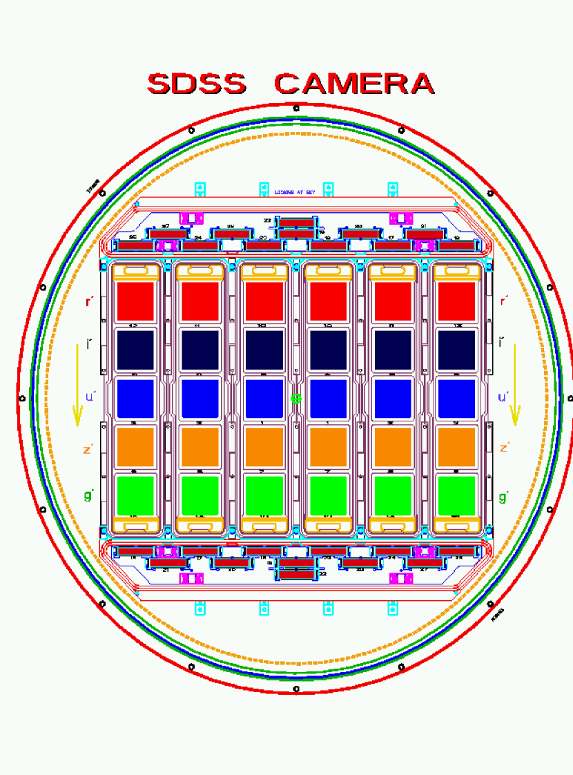
Figure 1: Layout of the Imaging Camera. The large colored squares represent the photometric CCDs, five in each of six dewars which run vertically on the page. The smaller rectangles above and below show the 22 astrometric and two focus CCDs in two dewars running horizontally. The arrows indicate the direction of motion of stars across the camera during a scan.

The imaging camera (Gunn et al., 1998, Figure 1) consists of 54 CCDs in eight dewars and spans $2.3\arcdeg$ on the sky. Thirty of these CCDs are the main imaging/photometric devices, each a SITe (Scientific Imaging Technologies, formerly Tektronix) device with 2048² – 24$\mu$m square pixels. They are arranged in six column dewars of five CCDs each, one CCD for each filter bandpass ($u\,g\,r\,i\,z$) in each column. The camera is operated in TDI (Time Delay and Integrate), or scanning, mode for which the telescope is driven at a rate synchronous with the charge transfer rate of the CCDs. Objects on the sky drift down columns of the CCDs so that five-color photometry is obtained over an interval of 5 minutes with no dead-time for shuttering and read-out. The effective integration time is 53.9 seconds at the chosen (sidereal) scanning rate (the pixel scale is 0.396 arcseconds per pixel).

The other 24 CCDs in two additional dewars are also SITe chips of width 2048 – 24$\mu$m pixels, but they have only 400 rows in the scanning direction. These dewars are oriented perpendicular to the photometric dewars, and one lies across the top of the columns, the other across the bottom. Each dewar contains 12 CCDs. Two of these CCDs (one in each dewar) are used to dynamically determine changes in focus. The other 22 CCDs are used to tie observations to an astrometric reference frame. They saturate at brighter magnitudes than the photometric CCDs because they (1) have a shorter integration time (10.5 seconds), since they have 400 versus 2048 rows in the scanning direction; (2) are behind a neutral density filter of 3.0 stellar magnitudes; and (3) have somewhat poorer quantum efficiency. The astrometric CCD filter bandpass is similar to the photometric $r$ bandpass, though it extends $\sim 400$ Å redwards of the $r$ red cutoff. The astrometric CCDs saturate at $r\simeq 8$, and thus can utilize all but the brightest 10% of the astrometric standard stars in Tycho-2. The photometric $r$ CCDs saturate at $r\simeq 14$, while good centroids may be measured on the astrometric CCDs for stars as faint as $r\simeq 17$. Hence there is an overlap of about 3 magnitudes between faint stars with good centroids on the astrometric chips and bright unsaturated stars on the $r$ chips, enabling the transfer of catalog stars detected on the astrometric CCDs to the $r$ CCDs, and thus the astrometric calibration of stars detected on the $r$ CCDs against bright reference catalogs. Similarly, there is an overlap of at least 5 magnitudes between stars with good centroids detected on the $r$ CCDs and the other photometric CCDs, allowing the $r$ astrometric calibrations to be transferred to the other photometric CCDs.

Twelve of the astrometric CCDs are aligned with the six columns of photometric CCDs, with an astrometric chip leading and trailing each column. The other 10 astrometric chips bridge the gaps between the columns. Hence the astrometric chips span the full 2.3$\arcdeg$ width of the camera. As outlined below, the bridge astrometric CCDs are not used in the current version of the astrometric pipeline. They were originally intended to account for differential shifts between the photometric dewars, but the camera has proven to be extremely stable and the technique was not needed.

3 Data Processing Overview

The large volume of data generated by the SDSS requires a set of automated data processing pipelines to acquire and archive the raw data, detect and measure object parameters, astrometrically and photometrically calibrate the objects, select spectroscopic targets, design the spectroscopic plates, extract spectra, and measure various spectral parameters. The end-to-end processing of SDSS data is discussed in detail in Stoughton et al. (2002). Those parts of data processing which are relevant to the astrometric calibrations are briefly summarized here to give context to the detailed discussion of the astrometric calibrations.

Each imaging drift scan is processed serially through the following pipelines:

1. The real-time Data Acquisition System (DA, Petravick et al., 1994) acquires the raw data as they are read off the CCDs, buffers them to disk, archives them to tape, and performs real-time quality analysis (it is the only real-time component of data processing). The data stream from each CCD is broken up into frames (2048 columns by 1361 rows) to facilitate data processing. DA finds bright stars on the frames from the astrometric CCDs, cuts out a 29 by 29 pixel (11.5 by 11.5 arcseconds) subraster (postage stamp) centered on each star, and measures parameters, including a centroid and flux, for each star (the astrometric frames are not saved).

2. The Serial Stamp Collection Pipeline (SSC, Lupton et al., 2001) cuts out postage stamps and measures centroids for bright stars on the photometric CCD frames. It measures stars at the expected positions based on the DA detections on the astrometric CCDs in the same camera column and includes a star finder to detect additional stars not detected on the astrometric CCDs.

3. The Postage Stamp Pipeline (PSP, Lupton et al., 2001) uses postage stamps for bright stars cut out by SSC to measure the point spread function (PSF) as a function of position across each frame (for the photometric CCDs only). The star centroids for all postage stamps are remeasured using an algorithm that corrects for asymmetries in the PSF, as described in Section 4.

4. The Astrometric Pipeline (Astrom) matches up the stars detected by DA for the astrometric CCDs, and/or those detected by SSC for the photometric CCDs with corrected centroids produced by PSP, to a primary astrometric reference catalog. Using these matches, it derives a separate set of transformation equations for each frame, converting frame row and column to J2000 catalog mean place celestial coordinates. This procedure provides the astrometric calibration for the SDSS, and is the topic of this paper. The pipeline itself is described in detail in Section 5.

5. The Imaging Pipeline (Frames, Lupton et al., 2001) corrects the raw frames for instrumental effects, detects objects on the corrected frames, matches up detections of the same object in different filters, deblends overlapping objects, and measures parameters for the objects. It uses the astrometric calibrations produced by Astrom to precisely match up the separate detections in the different filters for each object. This requires that Astrom run before Frames, and explains why the astrometric calibrations are based on centroids measured by PSP and DA, rather than on Frames’s centroids. Frames and PSP use the same centroiding algorithm. The final SDSS object positions are derived by applying the astrometric calibrations produced by Astrom to the centroids measured by Frames.

In summary, the astrometric calibrations are produced by Astrom, processing a single drift scan at a time, using centroids measured by DA and/or PSP and producing a set of transformation equations for each frame which are applied to centroids measured by Frames.

4 Centroids

An object’s centroid is defined as the first moment of its light distribution. Since this is a noisy estimate for most objects in the survey, the following technique is used to better estimate the centroid. First, an object’s image is smoothed using a two-dimensional Gaussian with an adaptive smoothing length scaled to the PSF in that frame. Quartic interpolation is used to find the maximum in a $3\times 3$ pixel subraster centered on the peak pixel in the smoothed image. This gives a biased estimate of the centroid in the presence of an asymmetric PSF. The Postage Stamp Pipeline (PSP) uses bright stars to determine the shape of the PSF as a smoothly varying function of CCD column and row for each frame. Thus, the PSF at the position of each object is determined to high accuracy. The centroid of the PSF at the position of the object is measured using both the first moment and quartic interpolation after smoothing by the PSF. The difference in centroids measured for the PSF using the two algorithms is a measure of the bias introduced by the use of the quartic interpolation algorithm. This bias is typically a few tens of mas, but can be as large as 100 mas. The difference is added to the quartic interpolation centroid measured for the object, yielding a high signal-to-noise ratio estimate of the first moment centroid of the object. A more detailed discussion of the centroiding algorithm will appear in the forthcoming paper on SDSS photometry (R. Lupton et al., in preparation).

PSP and Frames both use the bias-corrected centroiding algorithm described above. This is necessary because the astrometric calibrations are produced from centroids measured by PSP but are applied to centroids measured by Frames. Since neither DA nor SSC has an estimate of the PSF, they measure uncorrected quartic interpolation centroids, using a constant smoothing length of $\sigma=1.2$ pixels ($\sim 0.48$ arcseconds). When reducing against Tycho-2, Astrom uses DA’s uncorrected centroids for objects detected on the astrometric CCDs; however the biases thus introduced are largely removed in the calibrations and are small compared to more dominant atmospheric effects.

In addition to its row and column centroid, each detection of a star is characterized by the terrestrial time (TT) when the star was at mid-exposure, its flux on that frame, and an instrumental color based on detections on two CCDs in the same camera column during the same drift scan ($r\!-\!i$ for the $r$, $i$, $z$, and astrometric CCDs, $u\!-\!g$ for the $u$ CCDs, and $g\!-\!r$ for the $g$ CCDs). Astrom converts instrumental fluxes and colors to approximate calibrated magnitudes and colors using a separate zero point for each CCD (derived from a recent photometric calibration), the airmass at the middle of the frame, and average values for the extinction (0.520 mags per unit airmass in $u$, 0.200 in $g$, 0.120 in $r$, 0.080 in $i$, and 0.065 in $z$). These calibrated magnitudes are used by Astrom for quality analysis and to reject faint stars. The calibrated colors are used for differential chromatic refraction (DCR) calculations. The expected errors in the approximate magnitudes and colors do not contribute significantly to the overall astrometric error budget. Only unsaturated stars brighter than $20^{th}$ magnitude are used to derive the astrometric calibrations.

5 Calibrations

The $r$ CCDs serve as the astrometric reference CCDs for the SDSS. That is, the positions for SDSS objects are based on the $r$ centroids and calibrations. One of two reduction strategies is employed, depending on the coverage of astrometric catalogs:

1. Whenever possible, stars detected on the $r$ photometric CCDs are matched directly with stars in UCAC. UCAC extends down to $R=16$, giving approximately 2 – 3 magnitudes of overlap with unsaturated stars on the photometric $r$ CCDs. The astrometric CCDs are not used.

2. If UCAC coverage is not available to reduce a given imaging scan, detections of Tycho-2 stars on the astrometric CCDs are mapped onto the $r$ CCDs (all Tycho-2 stars saturate on the $r$ CCDs) using bright stars that have sufficient signal-to-noise ratio on the astrometric CCDs and are unsaturated on the $r$ CCDs. (This mode was originally expected to be the norm; at the time the camera was designed, UCAC was several years away from beginning observations.)

The $r$ CCDs are therefore calibrated directly against the primary astrometric reference catalog. Frames uses the astrometric calibrations to match up detections of the same object observed in the other four filters. The accuracy of the relative astrometry between filters can thus significantly impact Frames, in particular the deblending of overlapping objects, photometry based on the same aperture in different filters, and detection of moving objects. To minimize the errors in the relative astrometry between filters, the $u$, $g$, $i$, and $z$ CCDs are calibrated against the $r$ CCDs.

Each drift scan is processed separately. All six camera columns are processed in a single reduction. In brief, stars detected on the $r$ CCDs if calibrating against UCAC, or stars detected on the astrometric CCDs transformed to $r$ coordinates if calibrating against Tycho-2, are matched to catalog stars. Transformations from $r$ pixel coordinates to catalog mean place (CMP) celestial coordinates are derived using a running-means least-squares fit to a focal plane model, using all six $r$ CCDs together to solve for both the telescope tracking and the $r$ CCDs’ focal plane offsets, rotations, and scales, combined with smoothing spline fits to the intermediate residuals. These transformations, comprising the calibrations for the $r$ CCDs, are then applied to the stars detected on the $r$ CCDs, converting them to CMP coordinates and creating a catalog of secondary astrometric standards. Stars detected on the $u$, $g$, $i$, and $z$ CCDs are then matched to this secondary catalog, and a similar fitting procedure (each CCD is fitted separately) is used to derive transformations from the pixel coordinates for the other photometric CCDs to CMP celestial coordinates, comprising the calibrations for the $u$, $g$, $i$, and $z$ CCDs. The remainder of this section describes the calibration procedure in detail.

5.1 Great Circle Coordinates

In order to minimize curvature and time differences as objects drift across the focal plane, all SDSS drift scans are conducted along CMP J2000 great circles. Each such great circle (referred to as a stripe) is defined by the inclination and the right ascension of the ascending node where the great circle crosses the J2000 celestial equator (Stoughton et al. [2002] provides more information on the various coordinate systems employed in the survey). The boresight is defined as the position in the focal plane that nominally tracks the great circle. A minimum of two scans is required along each great circle, one with the boresight offset 22.74 mm below (perpendicular to the scan direction) the camera center (referred to as the north strip of the stripe), and one with the boresight offset 22.74 mm above the camera center (referred to as the south strip). The two strips are interlaced to fill in the gaps between the camera columns, such that two strips together cover a swath about $2.53\arcdeg$ wide centered along the great circle. The offsets between strips are chosen so that the individual scan lines from each of the six CCD columns overlap slightly ($\sim 0.5^{\prime}$) with adjacent scan lines when interlaced. Adjacent stripes, separated by $2.5\arcdeg$, also overlap at their edges. The boresight tracking rate is adjusted by the telescope control computer (TCC) to be constant in observed place.

Reductions are simplified by working in a coordinate system in which the tracked great circle is the equator of the coordinate system. In this coordinate system, referred to throughout as the great circle coordinate system, the latitude of an observed star never exceeds about $1.3\arcdeg$; thus the small angle approximation may be used and lines of constant longitude are to a high approximation perpendicular to lines of constant latitude. Longitude and latitude in great circle coordinates are referred to with the symbols $\mu$ and $\nu$, respectively. $\nu=0$ along the great circle, $\mu$ increases in the scan direction, and the origin of $\mu$ is chosen so that $\mu=\alpha_{2000}$ at the ascending node (where the great circle crosses the J2000 celestial equator). The conversion from great circle coordinates to J2000 celestial coordinates is then

$$tan(\alpha_{2000}-\mu_{0}) = [\sin(\mu-\mu_{0})\cos\nu\cos i-\sin\nu\sin i]/[\cos(\mu-\mu_{0})\cos\nu]$$ (1)

$$sin(\delta_{2000}) = \sin(\mu-\mu_{0})\cos\nu\sin i+\sin\nu\cos i$$ (2)

where $i$ and $\mu_{0}$ are the inclination and J2000 right ascension of the great circle ascending node, respectively ($\mu_{0}=95\arcdeg$ for all survey stripes ).

5.2 Pseudo-Catalog Place

As stated above, the telescope boresight tracks (or should track) a J2000 great circle in CMP. The distance of a star’s image from the boresight on the telescope focal plane is proportional to the difference in observed place between the star and the boresight pointing. The reductions are therefore performed in pseudo-catalog place (PCP), a nonstandard place defined as

$$\mu_{\ast,PCP} = \mu_{B,CMP}+(\mu_{\ast,OP}-\mu_{B,OP})$$ (3)

$$\nu_{\ast,PCP} = \nu_{B,CMP}+(\nu_{\ast,OP}-\nu_{B,OP})$$ (4)

where the subscripts $\ast$ and B indicate the star and boresight, respectively, and the subscripts PCP, CMP, and OP signify pseudo-catalog place, catalog mean place, and observed place, respectively (for definitions of various astrometric places, see Hohenkerk et al. [1992]). Local place could just as well have been used; however using pseudo-catalog place facilitates the generation of quality analysis information regarding the telescope tracking and camera rotation over the course of a scan. That is, the pipeline explicitly solves for parameters describing the actual telescope scanning.

5.3 Calibration Equations

While the reductions are performed in PCP, ultimately a transformation from pixel coordinates to CMP is required. Throughout all SDSS data processing, the data from each CCD in a drift scan are broken up into contiguous frames of 2048 columns (columns are parallel to the scan direction) by 1361 rows (perpendicular to the scan direction). Astrometric calibrations are generated as a separate set of equations for each frame converting frame row ($x$), frame column ($y$), and star color to CMP great circle coordinates ($\mu_{CMP}$, $\nu_{CMP}$).

$${\rm for}\ \hbox{$r\!-\!i$} < (\hbox{$r\!-\!i$})_{0}:$$ (6)

$$x^{\prime}=x+g_{0}+g_{1}y+g_{2}y^{2}+g_{3}y^{3}+p_{x}color$$

$$y^{\prime}=y+h_{0}+h_{1}y+h_{2}y^{2}+h_{3}y^{3}+p_{y}color$$

$${\rm for}\ \hbox{$r\!-\!i$} \geq (\hbox{$r\!-\!i$})_{0}:$$ (8)

$$x^{\prime}=x+g_{0}+g_{1}y+g_{2}y^{2}+g_{3}y^{3}+q_{x}$$

$$y^{\prime}=y+h_{0}+h_{1}y+h_{2}y^{2}+h_{3}y^{3}+q_{y}$$

$$\mu_{CMP} = a+bx^{\prime}+cy^{\prime}$$ (9)

$$\nu_{CMP} = d+ex^{\prime}+fy^{\prime}$$ (10)

The transformation from ($x$, $y$) to ($x^{\prime}$, $y^{\prime}$) corrects for optical distortions (which, in TDI mode, are a function of column only) and DCR. For $u$ and $g$ frames, DCR is modeled as a linear function of color ($u\!-\!g$ for $u$ frames, $g\!-\!r$ for $g$ frames) for stars bluer than $(\hbox{$r\!-\!i$})_{0}=1.5$, and a constant for redder stars. For $r$, $i$, and $z$ frames, DCR is modeled as a linear function of color ($r\!-\!i$) for all stars ($[\hbox{$r\!-\!i$}]_{0}=\infty$). The corrected frame coordinates ($x^{\prime}$, $y^{\prime}$) are then transformed to CMP great circle coordinates ($\mu_{CMP}$, $\nu_{CMP}$) using an affine transformation.

Figure 2 displays cubic polynomial fits to the observed optical distortions as a function of CCD column for each CCD. Distortions are typically less than 0.2 pixels, and are stable from month to month.

Figure 2: Cubic polynomial fits to the observed optical distortions for TDI scanning, in pixels, as a function of CCD column. Plots are displayed for each CCD (labelled by filter) in camera columns 1 – 6 (left to right) of the imaging camera. The distortions along the rows are plotted as solid lines, and along the columns as dotted lines.

The use of a set of transformation equations per frame, rather than directly calibrating each object, facilitates compartmentalization in data processing as well as later recalibrations. However, it can introduce systematic errors if the equations do not adequately map the true behavior. After fitting the optical distortion terms, there remain systematics as a function of column, though typically of order 5 mas or less. It is more difficult to estimate the errors introduced by the approximation that the astrometry changes linearly with time (that is, with row) over a single frame on the photometric CCDs; however they seem to be less than order 10 mas. (This is not a good approximation for the astrometric CCDs, for which the effects of seeing are more severe due to the shorter integration times.)

The equations for fitting DCR were determined by convolving spectrophotometry of stars from the Gunn & Stryker (1983) spectral atlas with the SDSS filter curves and a model atmosphere. For the $r$, $i$, and $z$ filters the linear fits of DCR versus color at a given airmass are excellent over all spectral types, with rms errors of less than 5 mas at a zenith distance of 60 degrees (the extreme zenith distance at which observations are obtained; as zenith distance is varied, the DCR errors scale with refraction). In $u$ and $g$ the linear fits are poorer but adequate if confined to stars bluer than $r-i\simeq 1.5$, with rms errors of 38 and 13 mas, respectively, at a zenith distance of 60 degrees. For redder stars the DCR terms in $u$ and $g$ are poorly behaved, and thus a constant value is employed. The accuracy of the astrometry, including the systematics introduced by the form of the transformation equations, is discussed in Section 6.

5.4 r Calibrations

The technique used to calibrate the $r$ CCDs depends on the primary standard star catalog used. The preferred catalog is UCAC, an (eventually) all-sky astrometric catalog with a precision of 70 mas at its catalog limit of $R\simeq 16$, and systematic errors of less than 30 mas. Currently the entire Southern Hemisphere has been observed, with partial coverage in the north (the entire sky should be finished by the end of 2003); one-third of the SDSS area is covered at present. There are 2 – 3 magnitudes of overlap between the faint end of UCAC and bright unsaturated stars on the $r$ CCDs (depending on the CCD and on seeing), allowing the direct calibration of the $r$ CCDs against UCAC, bypassing the astrometric CCD to photometric CCD bootstrap.

If a scan is not covered by the current UCAC catalog, then it is reduced against Tycho-2, an all-sky astrometric catalog with a median precision of 70 mas at its catalog limit of $V_{T}\simeq 11.5$, and systematic errors of less than 1 mas. All Tycho-2 stars are saturated on the $r$ CCDs; however there are about 3.5 magnitudes of overlap between bright unsaturated stars on the astrometric CCDs and the faint end of Tycho-2 ($8<r<11.5$), and about 3 magnitudes of overlap between bright unsaturated stars on the $r$ CCDs and faint stars on the astrometric CCDs ($14<r<17$). For reductions against Tycho-2, the star centroids on the astrometric CCDs are transformed to the pixel coordinates of the $r$ CCD in the same column using the unsaturated stars detected on both the astrometric and $r$ CCDs. Each pair of astrometric-$r$ CCDs is processed separately. Stars on each astrometric CCD are matched to stars on its associated $r$ CCD. There are typically 10 – 20 matched pairs per frame. For each frame, the nearest (in $\mu$) 30 matched pairs, including all matched pairs on that frame, are used to derive an affine transformation from the astrometric CCD pixel coordinate system to the $r$ CCD pixel coordinate system, minimizing the rms row and column differences between the astrometric and $r$ stars. If this is the first fitting iteration, outliers are rejected. Smoothing splines, using three piecewise polynomials per frame, are then fitted to the row and column residuals as a function of row (time). Outliers are rejected, and the fitting process is iterated two more times. Finally, the remaining residuals for all matched pairs are fitted, using a least-squares fit to a cubic polynomial, as a function of column to remove the optical distortions. The resultant solution is used to transform the stars detected on the astrometric CCD to the pixel coordinate system of the $r$ CCD. If a star was detected on both the leading and trailing astrometric CCDs within a column, then its transformed $r$ coordinates are averaged and the mean position is used. These transformed stars will then be matched to the Tycho-2 stars to yield a transformation from $r$ pixel coordinates to great circle CMP coordinates.

Figure 3: Typical smoothing spline fits for the transformation from an astrometric CCD to an $r$ CCD. The 20 frames displayed is approximately 12 minutes of data.

Figure 3 shows a typical smoothing spline fit to the row and column residuals for an astrometric CCD to $r$ CCD match. The difficulty in doing astrometry with 11 second exposures in drift scan mode is evident. Peak-to-peak excursions are 100 – 300 mas, with time scales of order half a frame (18 seconds). These most likely are due to anomalous refraction (see Section 6.4). The scan used for the plot has a higher number of pairs per frame than most scans, with half that number more typical. While no all-sky astrometric catalog of sufficient accuracy is dense enough to follow the atmospheric excursions on these time scales, there are enough overlap stars between the astrometric and $r$ CCDs to allow most of the systematics to be removed. There is a tendency for the peaks of the excursions to be underfitted. Interpolating splines were experimented with in place of the smoothing splines, but the final astrometry was not improved. The rms residual in either row or column for the transformation from an astrometric CCD to an $r$ CCD is typically 30 – 50 mas.

The reduction now proceeds similarly whether reducing against UCAC or Tycho-2. The following focal plane model is used, relating frame row ($x$) and column ($y$) to PCP coordinates (the small angle approximation is assumed for all rotations).

$$x^{\prime} = x+g_{0}+g_{1}y+g_{2}y^{2}+g_{3}y^{3}$$ (11)

$$y^{\prime} = y+h_{0}+h_{1}y+h_{2}y^{2}+h_{3}y^{3}$$ (12)

$$\mu_{\ast,PCP} = \mu_{B,CMP}+T_{\mu}x^{\prime}+s[X_{CCD}-X_{B}+(Y_{CCD}-Y_{B})\theta_{CAM}$$

$$+0.024f_{CCD}(y^{\prime}-1024)(\theta_{CAM}+\theta_{CCD})]$$

$$\nu_{\ast,PCP} = \nu_{B,CMP}+T_{\nu}x^{\prime}+s[-(X_{CCD}-X_{B})\theta_{CAM}+Y_{CCD}-Y_{B}$$

$$+0.024f_{CCD}(y^{\prime}-1024)]$$

$x^{\prime}$ and $y^{\prime}$ are frame row and column corrected for optical distortions. The telescope tracking (along the CMP great circle) is modeled by specifying the boresight pointing when row 0 of the frame was read ($\mu_{B,CMP}$ and $\nu_{B,CMP}$, in arcseconds) and the tracking rate parallel ($T_{\mu}$, in arcseconds pixel^-1) and perpendicular ($T_{\nu}$) to the great circle. A perfectly tracked scan would have $\nu_{B,CMP}=0$, $T_{\nu}=0$, and $T_{\mu}$ equal to the sidereal rate. The location of the telescope boresight in the focal plane is specified by the constant parameters $X_{B}$ (always set to 0) and $Y_{B}$ (-22.74 mm for north strips, +22.74 mm for south strips). $s$ is the telescope scale (in arcseconds mm^-1) and $\theta_{CAM}$ the rotation of the camera from its correct value (in radians). $X_{CCD}$ and $Y_{CCD}$ are the location of the center of the CCD (column 1024) in the focal plane (in mm), $\theta_{CCD}$ is the rotation of the CCD with respect to the focal plane coordinate system, $f_{CCD}$ is the relative scale of the CCD (with nominal value of 1), and the size of the pixels is 0.024 mm. $\mu_{\ast,PCP}$ and $\nu_{\ast,PCP}$ are the resultant PCP coordinates of the star (in arcseconds).

The camera geometry (the telescope scale and the CCD focal plane locations, rotations, relative scales, and optical distortion terms) is calibrated once a month using a scan through a UCAC field. (Before UCAC became available, calibration regions measured using the Flagstaff Astrometric Scanning Transit Telescope [Stone, 1997; Stone, Pier, & Monet, 1999, FASTT;] were used.) The most recent set of these nominal values is used as an initial (and in some cases final) guess at those values for the current reduction. The CCD terms are stable from month to month.

The focal plane model, initialized using the TCC telescope tracking information and a recent calibration scan, is first used to calculate a priori CMP coordinates for each observed star (stars detected on the $r$ CCDs for reductions against UCAC, and stars detected on the astrometric CCDs and converted to the $r$ pixel coordinate systems for reductions against Tycho-2). These a priori coordinates are used to match the observed stars with the catalog stars (catalog stars whose catalog error in either right ascension or declination exceeds 60 mas are not used, rejecting about 25% of the stars). For each matched pair, the position of the catalog star is converted from CMP to PCP using the TT at mid-exposure for the observed star and the color of the star. UCAC does not contain color information, so the observed color ($r\!-\!i$) of the star is used for reductions against UCAC. Tycho-2 stars saturate the photometric CCDs and therefore do not have SDSS colors; thus the Tycho-2 catalog colors ($B_{T}\!-\!V_{T}$) are used, converted to $r\!-\!i$ using the transformation

$$\hbox{$r\!-\!i$}=-0.186+0.681(\hbox{$B_{T}\!-\!V_{T}$})-0.534(\hbox{$B_{T}\!-\!V_{T}$})^{2}+0.319(\hbox{$B_{T}\!-\!V_{T}$})^{3}.$$ (15)

A solution to the focal plane model is now derived for each frame, in order to minimize the rms differences in $\mu_{PCP}$ and $\nu_{PCP}$ between the observed and catalog stars. First, a separate linear least-squares fit is performed for each set of six frames observed at the same time by the six $r$ CCDs. The CCD terms (focal plane locations, scales, rotations, and optical distortions) are held constant at their nominal values, and only the six terms specifying the boresight tracking ($\mu_{B,CMP}$, $\nu_{B,CMP}$, $T_{\mu}$, and $T_{\nu}$), telescope scale ($s$), and camera rotation ($\theta_{CAM}$) are fitted. For a given set of six frames, all matched pairs on that set of frames are used. Additional matched pairs from the nearest adjacent frames are used if required to yield a minimum number of matched pairs (30 for reductions against UCAC, 15 for reductions against Tycho-2). If an adjacent set of frames is used, then all matched pairs on that set of frames are used. For reductions against UCAC, there are typically 3 – 10 catalog stars per frame, so it is usually not necessary to use the adjacent frames. For reductions against Tycho-2, there is typically one catalog star every two frames; thus it is generally necessary to use the adjacent four or more sets of frames to achieve the minimum number of pairs.

If this is the first iteration, outliers are rejected. There are systematics remaining in the residuals after the least-squares fit, primarily due to anomalous refraction, varying with typical time scales of 5 – 20 frames (see Section 6.4). For reductions against UCAC, smoothing splines are fitted to the $\mu$ and $\nu$ residuals for each $r$ CCD separately, with breakpoints separated by five frames. This is not possible for reductions against Tycho-2, due to the paucity of catalog stars. Rather, the average (over the entire scan) residual in $\mu$ and $\nu$ is removed for each $r$ CCD separately. In either case, this procedure effectively refits the CCD location in the focal plane ($X_{CCD}$ and $Y_{CCD}$). For both the UCAC and Tycho-2 case, outliers are rejected, and the process of the least-squares fit, spline fits, and outlier rejection is iterated two more times.

Figure 4: Typical smoothing spline fits for the transformation from $r$ CCDs to UCAC.

Figure 4 shows typical smoothing spline fits to the $\mu$ and $\nu$ residuals for all six $r$ CCDs for part of a reduction against UCAC (separate fits for each CCD). Systematics in common to all six CCDs (such as due to telescope jitter or any portion of anomalous refraction which is correlated across the focal plane) have already been removed by the running-means. The remaining systematics have typical amplitudes of 20 mas, with time scales of a few frames or more. There are occasional features with time scales closer to a frame, which are more prevalent in worse seeing. The spline fits remove most of the systematics but not all. More closely placed breakpoints have been experimented with, but this can lead to fitting features that are not real. The chosen breakpoint separation of five frames is a good compromise between fitting most of the real features without overfitting the data for typical seeing conditions. These systematics cannot be removed for reductions against Tycho-2, as there are too few catalog stars detected per CCD to map the systematics. This adds roughly 10 – 20 mas in quadrature to the rms errors for reductions against Tycho-2. Similarly, the running-means typically smoothes over single frames for reductions against UCAC, and five frames for reductions against Tycho-2. Thus, any correlated systematics with time scales of order a frame cannot be removed from reductions against Tycho-2.

For reductions against UCAC, the optical distortion terms ($g_{i}$, $h_{i}$) are then refitted by fitting the remaining residuals to a cubic polynomial as a function of column. One set of terms is calculated per CCD for the entire scan, not per frame. This effectively refits the CCD rotations and relative scales ($\theta_{CCD}$ and $f_{CCD}$ in the focal plane model). There are not enough matched pairs for a reduction against Tycho-2, particularly for short scans, to refit these terms, so the nominal values from the most recent calibration scan are used. While these terms are very stable over time, occasionally there is evidence of residual CCD rotation or scale changes.

The solution is a transformation (nonlinear in row) from $r$ pixel coordinates to PCP coordinates. This needs to be converted to the calibration equations of Section 5.3, which convert from pixel coordinates to CMP coordinates, one set of equations per frame. The optical distortion terms of the solution are copied directly to the calibration equations. For each frame, PCP coordinates are calculated from the solution at the midpoint of each of the four sides of the frame. These are converted to CMP using the TT at mid-exposure and assuming a star of zero color. These four test points then determine the affine transformation portion of the calibration equations. The CMP is similarly calculated for 11 test points all located in the middle of the frame but spanning a range in color. The $\mu_{CMP}$ and $\nu_{CMP}$ offsets from a star of zero color are then fitted as linear functions of color, yielding the DCR terms for each frame.

5.5 $u$, $g$, $i$, and $z$ Calibrations

The $r$ calibration equations are applied to all the stars detected on the $r$ CCDs, generating CMP positions for these stars. This creates a catalog of secondary astrometric standards which is used to calibrate the remaining photometric CCDs. Each of the $u$, $g$, $i$, and $z$ CCDs is calibrated separately. The stars detected on a given CCD are matched against the secondary catalog from the $r$ CCD in the same camera column. There are typically 10 – 40 matched pairs per frame (5 – 20 on the $u$ CCDs). For each matched pair, the position of the catalog star is converted from CMP coordinates to PCP coordinates using the TT at mid-exposure and the color ($u\!-\!g$ for $u$, $g\!-\!r$ for $g$, $r\!-\!i$ for $i$ and $z$) of the observed star. For each frame all matched pairs on that frame are used to derive an affine transformation from pixel coordinates to PCP coordinates, minimizing the rms differences in $\mu_{PCP}$ and $\nu_{PCP}$ between the observed and catalog stars. If there are fewer than 15 matched pairs on the frame, then the nearest matched pairs on adjacent frames are used to guarantee that a minimum of 15 pairs is used. Outliers are rejected, and the process of fitting and outlier rejection is iterated two more times. The remaining residuals for all matched pairs are fitted using a least-squares fit to a cubic polynomial as a function of column to remove the optical distortions (that is, one polynomial is fitted per CCD for the entire scan, not each frame). Chromatic aberration in the optics can produce systematics with color in the remaining residuals. This is significant only in $g$. Thus, for $g$ only, an empirically determined linear term with color (based on a fit to a single scan, but which has proven to be stable from scan to scan) is removed from the remaining residuals. The resulting solution transforms pixel coordinates to PCP coordinates. It is converted to the calibration equations of Section 5.3, which convert from pixel coordinates to CMP coordinates, using the same procedure used for the $r$ CCDs.

6 Results

This section quantifies the accuracy of the astrometric calibrations. The calibrations are based on stars brighter than $20^{th}$ magnitude, for which centroiding errors are negligible (except in the $u$ filter, where the centroiding errors start to become significant by $20^{th}$ and contribute to the rms errors quoted here). Thus, the accuracies quoted here are for the calibrations only, and reflect the astrometric accuracy expected for stars brighter than $20^{th}$. Centroiding errors (which are calculated by Frames) must also be considered for fainter stars and all galaxies, and are discussed at the end of the section. The results presented here are based on the entire SDSS data set to be made public in early 2003 as SDSS Data Release 1 (DR1). This includes 33 scans covering roughly 1200 square degrees of sky (not all unique) reduced against UCAC, and 32 scans covering roughly 750 square degrees of sky reduced against Tycho-2. The distribution of internal residuals within a single scan, the distribution of differences in position for matched pairs between two runs, and the distribution of differences in position for the SDSS matched against the external catalogs used in this analysis are all well characterized by Gaussians, and therefore by rms residuals and differences. Thus all errors are quoted as rms residuals or differences in $\mu$ and $\nu$.

6.1 r Astrometry

The absolute accuracy of the $r$ astrometry is difficult to gauge, as there are no astrometric catalogs as deep and accurate as the SDSS itself. The primary internal measure of the precision of the astrometry is the distribution of residuals (measured position of the SDSS object minus the catalog position) for matched pairs (after outlier rejection) on the $r$ CCDs. Figure 5 shows histograms of these residuals for all matched pairs for reductions against UCAC and Tycho-2 separately. The rms residuals per coordinate are 45 mas and 75 mas for reductions against UCAC and Tycho-2, respectively.

Figure 5: Histograms of the residuals (SDSS position minus catalog position) for scans reduced against UCAC (a) and scans reduced against Tycho-2 (b). The solid and dotted histograms are for the $\mu$ and $\nu$ residuals, respectively.

Figure 6: Histograms of the rms residuals (SDSS position minus catalog position) for each frame in scans reduced against UCAC (a) and scans reduced against Tycho-2 (b). The rms residuals for each frame are calculated using a minimum of the nearest 100 matched pairs. The solid and dotted histograms are for the $\mu$ and $\nu$ rms residuals, respectively.

Figure 7: Median rms residual per frame binned by seeing for the $r$ CCDs. Triangles are for the $\mu$ residuals, squares the $\nu$ residuals. Open symbols are for reductions against UCAC, filled symbols are for reductions against Tycho-2.

Figure 8: Histograms of the position differences for matched pairs on overlapping scans. Results from reductions against UCAC are shown in panel a, those for reductions against Tycho-2 in panel b. The solid and dotted histograms are for the $\mu$ and $\nu$ differences, respectively.

The precision, of course, can vary from scan to scan, and during individual scans. For each scan the rms residuals (around 0) in $\mu$ and $\nu$ are calculated separately for each frame, for each $r$ CCD separately. To assure good statistics, a smoothing window is used, using enough adjacent frames to give a minimum of 100 matched pairs per frame. These rms residuals in $\mu$ and $\nu$ for each frame are recorded with the calibration equations for that frame, and serve as the best estimate of the systematic errors for that frame. Figure 6 shows histograms of these rms residuals for all frames in DR1. All the distributions peak near the rms values indicated in Figure 5. For reductions against UCAC almost all frames have rms residuals of less than 60 mas. The distributions for reductions against Tycho-2 are broader, with most frames having rms residuals of less than 100 mas. The dependence on seeing is shown in Figure 7, which plots the median rms residual per frame binned by seeing (as measured by PSP). The reductions against Tycho-2 are considerably more sensitive to seeing than the reductions against UCAC, demonstrating that the longer integration times on the $r$ chips (relative to the astrometric chips), coupled with the greater star density of the UCAC catalog, are sufficient to remove most of the atmospheric effects.

Some parts of the sky have been scanned multiple times. Stars in nine pairs of overlapping scans (including some non-DR1 scans), reduced both against UCAC and Tycho-2, have been matched. The distribution of position differences for all matched pairs is shown in Figure 8. The rms differences are about 50 mas in both $\mu$ and $\nu$ for reductions against UCAC, and 73 mas in $\mu$ and 85 mas in $\nu$ for reductions against Tycho-2. These are smaller than one might expect from simply adding the internal errors in quadrature. Errors in UCAC and Tycho-2 catalog positions, which propagate to SDSS positions calibrated using those catalogs, are correlated among the repeat scans and thus are partially removed when differences in the SDSS positions are computed. Variation of astrometric precision within and between scans can be tested by sorting the matched pairs by $\mu$ and binning them into groups of 100, separately for each $r$ CCD. The rms differences in $\mu$ and $\nu$ are then calculated for each set of 100 matched pairs. Figure 9 shows histograms of these rms differences. For reductions against UCAC, the distributions peak around 45 mas, with most of the data having rms differences of less than 70 mas. For reductions against Tycho-2 the distributions are fairly broad, with typical rms differences of 60 mas, and most of the data having rms differences of less than 130 mas.

An external measure of the accuracy of the $r$ astrometry for data reduced against Tycho-2 may be obtained by re-reducing those scans which were reduced against UCAC against Tycho-2, and matching the resultant star positions against UCAC. Histograms of the position differences for all matched pairs are shown in Figure 10. The rms differences are 76 mas in $\mu$ and 79 mas in $\nu$, consistent with the internal rms residuals (Figure 5). There are mean offsets of -15 mas in $\mu$ and 18 mas in $\nu$. These are likely due to uncorrected magnitude terms in star positions on the SDSS astrometric CCDs, due to charge transfer efficiency (CTE) effects (seen by matching the leading and trailing astrometric CCDs in a given camera column), though residual magnitude terms in the preliminary UCAC catalog used may also contribute. The astrometric CCD magnitude terms are not currently corrected as 1) the necessary test data are lacking, and 2) UCAC coverage should be full-sky within a year, allowing all SDSS data to be recalibrated against UCAC, bypassing the astrometric CCDs. Again, variation of astrometric accuracy within and between scans can be tested by sorting the matched pairs by $\mu$ and binning them into groups of 100, separately for each $r$ CCD. The rms differences in $\mu$ and $\nu$ are then calculated for each set of 100 matched pairs. Histograms of these rms differences are plotted in Figure 11. The distributions are similar to the histograms for the rms internal residuals (Figure 6), peaking at 70 mas, though with a somewhat larger fraction of the data with rms differences exceeding 100 mas.

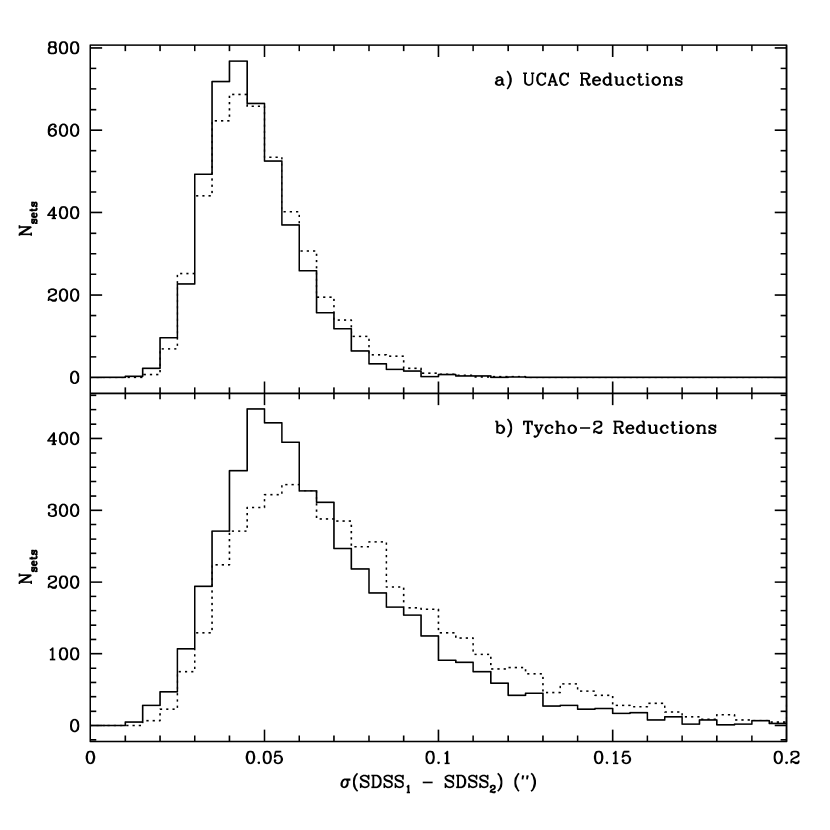
Figure 9: Histograms of the rms position differences for sets of 100 matched pairs between overlapping scans. For each pair of overlapping scans and for each $r$ CCD the matched pairs are sorted by $\mu$ and binned into groups of 100 matched pairs, and the rms differences in $\mu$ and $\nu$ are calculated for each set of 100 matched pairs. Results from reductions against UCAC are shown in panel a, those for reductions against Tycho-2 in panel b. The solid and dotted histograms are for the $\mu$ and $\nu$ rms differences, respectively.

Figure 10: Histograms of the position differences for matched pairs for reductions against Tycho-2 matched against UCAC. The solid and dotted histograms are for the $\mu$ and $\nu$ differences, respectively.

Figure 11: Histograms of the rms position differences for sets of 100 matched pairs, binned in $\mu$, for reductions against Tycho-2 matched against UCAC. For each scan and for each $r$ CCD the matched pairs are sorted by $\mu$ and binned into groups of 100 matched pairs, and the rms differences in $\mu$ and $\nu$ are calculated for each set of 100 matched pairs. The solid and dotted histograms are for the $\mu$ and $\nu$ rms differences, respectively.

Figure 12: Histograms of the position differences for matched pairs between the SDSS and 2MASS for nine scans. Results from reductions against UCAC are shown in panel a, those for reductions against Tycho-2 in panel b. The solid and dotted histograms are for the $\mu$ and $\nu$ differences, respectively.

The external catalog which most closely matches the SDSS in terms of depth, accuracy, and sky coverage is the Two Micron All Sky Survey (2MASS, Skrutskie et al., 1997). Typical position errors for the 2MASS Second Incremental Release are quoted as about 140 mas, though those are probably overstated and a truer measure of the rms errors may be closer to 110 mas (Cutri et al., 2000). Figure 12 shows histograms of the differences between the SDSS and 2MASS positions for stars in nine scans. 2MASS sources were limited to non-confused, non-extended sources detected in all three bands with $J<15.8$, $H<15.1$, and $K<14.3$, and with the major axis of the position error ellipse less than 175 mas. The rms differences are 118 mas in $\mu$ and 114 mas in $\nu$ for SDSS data reduced against UCAC, and 123 mas in $\mu$ and 122 mas in $\nu$ for SDSS data reduced against Tycho-2. These values are roughly what one would expect by combining the rms errors in the two catalogs in quadrature. There are mean offsets of -25 mas in $\mu$ and -58 mas in $\nu$ for SDSS reductions against UCAC, and -35 mas in $\mu$ and -33 mas in $\nu$ for SDSS reductions against Tycho-2. While the offsets in $\mu$ could be explained by systematic errors in the SDSS reductions, the $\nu$ offsets cannot. Similar offsets in $\nu$ are seen when matching UCAC against 2MASS in the same region of sky. A known bias exists in the 2MASS Second Incremental Release reductions whereby the positions of bright stars ($K\lesssim 9$), which are processed through the $R1$ path of the 2MASS pipeline, can be offset from those of fainter stars, which are processed through the $R2-R1$ path of the 2MASS pipeline; this bias will be addressed in the next 2MASS data release (H. L. McCallon 2001, private communication). This bias is likely the largest contributor to the $\nu$ offsets between the SDSS and 2MASS, and may also contribute to the $\mu$ offsets. (An earlier comparison between SDSS and 2MASS astrometry, based on a smaller data set, is presented by Finlator et al. [2000].)

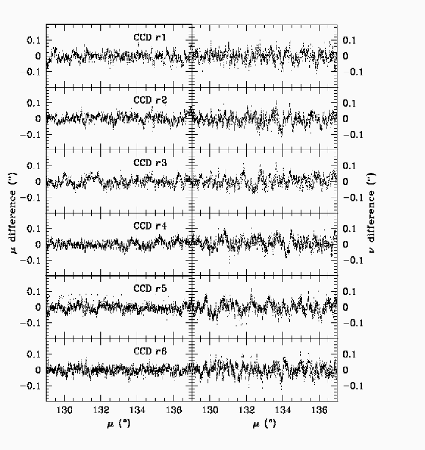
Figure 13: Differences in position between matched stars in two overlapping scans reduced against UCAC plotted against $\mu$ (time). The $\mu$ and $\nu$ differences are plotted separately for each $r$ CCD.

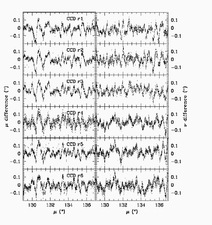
Figure 14: Same as Figure 13, but these data have been reduced against Tycho-2.

It should be emphasized that the values of the rms residuals and differences quoted characterize the distribution of systematic errors. The analysis is based on stars with $r<20$, for which random centroiding errors are small compared to the systematic errors. Figure 13 displays the differences in $\mu$ and $\nu$ between matched stars in two overlapping scans reduced against UCAC plotted against $\mu$ (time). The $\mu$ and $\nu$ differences are plotted separately for each $r$ CCD. Figure 14 shows the differences for matches for the same portion of the same overlapping scans, but reduced against Tycho-2. The differences vary systematically with time, on time scales of order one to a few minutes. While the differences are mostly uncorrelated between CCDs for the reductions against UCAC, they are strongly correlated for the reductions against Tycho-2. There are simply too few Tycho-2 stars to adequately follow the tracking errors and that portion of anomalous refraction which is correlated across the camera on short time scales. These plots are typical, and display well the nature of the dominant systematics in the astrometry.

SDSS astrometry is subject to any systematics present in the primary astrometric reference catalog. At the current epoch, systematics in Tycho-2 are expected to be less than a few mas, and as such do not degrade the overall accuracy of SDSS astrometry. Uncorrected magnitude terms in the star positions on the astrometric CCDs, used to transfer the Tycho-2 stars to the photometric CCDs, introduce systematic offsets between the Tycho-2 frame and SDSS data reduced against Tycho-2 of order 20 mas. A preliminary, internal version of UCAC (r07) is currently being used for SDSS astrometric reductions. This version of the catalog contains some uncorrected magnitude terms, such that the brighter stars, which are used to calibrate UCAC against Tycho-2, may be systematically offset from the fainter stars, which are used to calibrate the SDSS. Such offsets are thought to be of order 10 to 20 mas, mainly caused by residual CTE effects in the CCD used for the UCAC observations. In addition there will be zeropoint errors due to the fact that a given UCAC frame can only be linked with a certain accuracy to the Tycho-2 stars, depending on the number of reference stars available in that area of the sky. This will cause systematic errors of up to 30 mas on the 0.5 to 1 degree scale. Since UCAC uses only a single bandpass, colors for the stars were not available and DCR corrections could not be applied. However, the narrow bandpass used causes only 5 to 10 mas of systematic errors as a function of spectral type and zenith distance. In sum, total systematic errors in UCAC are thought not to exceed 30 mas (N. Zacharias 2001, private communication). As newer versions of UCAC with smaller systematic errors become available, the SDSS astrometry will be recalibrated.

6.2 $u$, $g$, $i$, and $z$ Astrometry

The primary internal measure of the accuracy of the relative astrometry between filters is the distribution of residuals (measured positions in the target filter – $u$, $g$, $i$, or $z$ – minus the measured positions in the $r$ filter). Figure 15 shows histograms of these residuals for all matched pairs (the relative astrometry between filters is not sensitive to the choice of primary reference catalog), separately for each filter. The relative astrometry is best in the $g$ and $i$ filters, with rms residuals of about 24 mas per coordinate. The $z$ filter is only slightly worse, with rms residuals of about 27 mas per coordinate. The centroids are poorer in the $u$ filter due to the lower flux for the stars used to derive the transformations, leading to larger rms residuals of about 33 mas per coordinate. Again, the variation in astrometric accuracy can be examined by calculating rms values for each frame, for each CCD pair. To assure good statistics, a smoothing window is used, using enough adjacent frames to give a minimum of 100 matched pairs per frame. The rms residuals in $\mu$ and $\nu$ for each frame are recorded with the calibration equations for that frame, and serve as the best estimate of the systematic error for that frame. Figure 16 shows histograms of these rms residuals. The distributions are fairly narrow in $g$, $i$, and $z$, with most frames having rms residuals of less than 35 mas. The distribution in $u$ shows a tail out to 60 mas. This is due both to the increased centroiding errors in the stars used to calibrate the $u$ frames, as well as to an occasional lack of enough bright stars to adequately calibrate the frame. The rms residuals are sensitive to seeing, as shown in Figure 17, which plots the median rms residual per frame binned by seeing.

Figure 15: Histograms of the residuals (SDSS position in the specified filter minus SDSS position in the $r$ filter) for all DR1 scans. The solid and dotted histograms are for the $\mu$ and $\nu$ residuals, respectively.

Figure 16: Histograms of the rms residuals (SDSS position in the specified filter minus SDSS position in the $r$ filter) for each frame in all DR1 scans. The rms residuals for each frame are calculated using a minimum of the nearest 100 matched pairs. The solid and dotted histograms are for the $\mu$ and $\nu$ rms residuals, respectively.

Figure 17: Median rms residual per frame binned by seeing for the $u$, $g$, $i$, and $z$ CCDs. Triangles are for the $\mu$ residuals, squares the $\nu$ residuals.

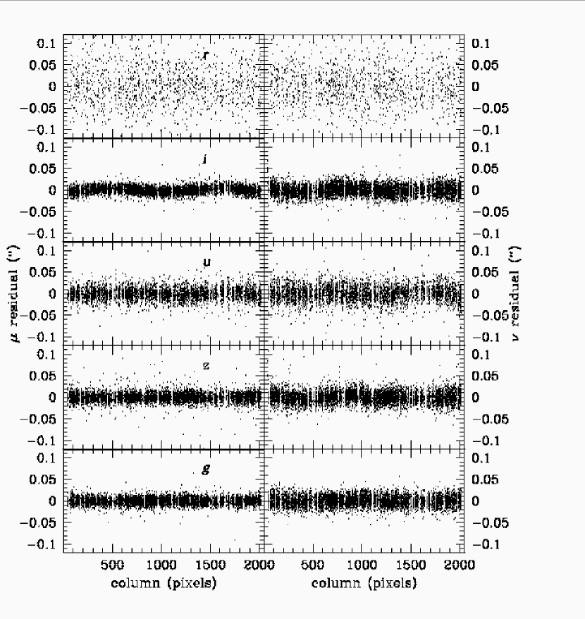
Figure 18: $\mu$ and $\nu$ residuals plotted against CCD column for all five photometric CCDs in column 3 of the camera for a scan taken under exceptional seeing. The scatter for the $r$ CCD is larger than the other CCDs because $r$ has been matched against UCAC while the other CCDs were matched against the $r$ detections.

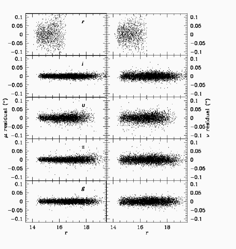
Figure 19: Same as Figure 18, but plotted against magnitude.

Figure 20: Same as Figure 18, but plotted against color ($r-i$ for $r$, $i$, and $z$, $u-g$ for $u$, and $g-r$ for $g$.

Figures 18, 19, and 20 plot the $\mu$ and $\nu$ residuals against CCD column, magnitude, and color, respectively, for all five photometric CCDs in column 3 of the camera for a scan taken under exceptional seeing to minimize the random errors and thus make any remaining systematic errors more obvious. The scatter for the $r$ CCD is larger than the other CCDs because $r$ has been matched against UCAC while the other CCDs were matched against the $r$ detections. Systematics with column (uncorrected by the cubic polynomials used to remove the optical distortions) are almost always less than 10 mas (though for some $u$ CCDs they can peak at 15 mas), and typically are 5 mas or less. Systematics with magnitude are always less than 13 mas over the magnitude range $14<r<22$, and are typically less than half that. Systematics with color are evident only for the $u$ and $g$ CCDs, and are typically less than 10 mas over the full range in color. All of these uncorrected systematics contribute to the rms residuals quoted above.

6.3 Centroiding Errors

The results presented above apply to stars brighter than $r\sim 20$, where systematic errors dominate centroiding errors, and thus characterize the errors in the calibrations. Centroiding errors become significant for stars fainter than $r\sim 20$, and for all galaxies. Figure 21 shows, in the upper two panels, the position differences against $r$ for matched stars between two overlapping scans reduced against UCAC. Each scan was taken under fairly constant seeing of $1.4\arcsec$ (the median seeing for all DR1 data is about $1.4\arcsec$). The errors clearly increase for stars fainter than $r\sim 20$. The position errors as a function of magnitude for a run taken during seeing of $1.4\arcsec$ can be estimated by binning the position differences in magnitude and calculating the rms differences in each magnitude bin, and dividing the rms by $\sqrt{2}$. This has been done in the lower panels of Figure 21. The rms errors increase from about 40 mas at $r\sim 20$ to about 100 mas at the survey limit of $r\sim 22$. The errors are seeing dependent, with rms errors at $r\sim 22$ ranging from about 70 mas to 140 mas in seeing of approximately $1.1\arcsec$ and $1.7\arcsec$, respectively (a range of seeing which characterizes most of the DR1 data).

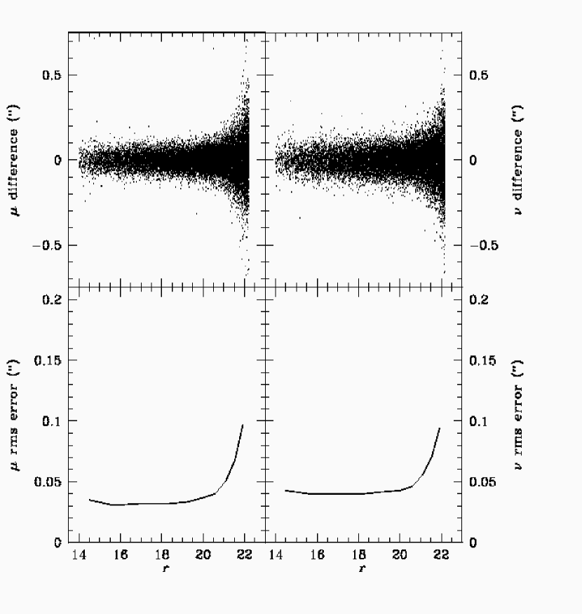
Figure 21: Position differences for stars plotted against $r$ for two overlapping scans (upper panels), and the rms position errors versus $r$ for stars for a typical scan (taken under $1.4\arcsec$ seeing), calculated from the position differences (lower panels).

Figure 22: Same as Figure 21, but for galaxies.

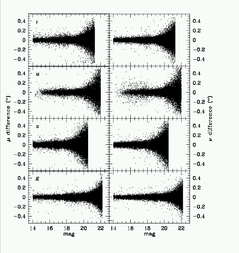
Figure 23: Position differences between the $i$, $u$, $z$, and $g$ filters, and the $r$ filter, plotted against magnitude ($i\,u\,z\,g$) for a typical scan.

Figure 24: Rms errors for the relative astrometry between the $i$, $u$, $z$, and $g$ filters, and the $r$ filter, plotted against magnitude ($i\,u\,z\,g$) for a typical scan.

Figure 22 is similar to Figure 21, but plots the position differences and estimated errors for galaxies rather than stars (for the same scans). Centroiding errors dominate the calibration errors even at bright magnitudes, with the rms errors ranging from about 60 mas at $r\sim 17$ to 170 mas at $r\sim 22$. These results are independent of seeing.

The accuracy of the relative astrometry between filters similarly decreases with increasing magnitude. Figure 23 plots the position differences between the $i$, $u$, $z$, and $g$ filters and the $r$ filter against magnitude ($i\,u\,z\,g$) for a single scan observed in $1.65\arcsec$ seeing. The rms errors as a function of magnitude can be calculated for this scan by binning the differences in magnitude and calculating the rms differences in each magnitude bin. These errors are shown in Figure 24. The rms errors increase to around 100 – 130 mas by the survey limits.

6.4 Anomalous Refraction

The primary contributions to systematic astrometric residuals appear to come from one or both of two causes: atmospheric fluctuations and/or telescope jitter. These observed systematics display considerable coherence across the focal plane; that is, both the direction and amplitude of the residuals from CCD to CCD show a high degree of correlation. These effects can be seen in Figures 13 and 14. The focal plane subtends $2.3\arcdeg$ across the sky and the physical dimension is on the order of $50$ cm (i.e., several times typical values for $r_{0}$).

Thus, one is led to believe that either the focal plane itself is moving (due, e.g., to telescope jitter) or the atmosphere is coherently moving the telescope beam. These two effects are difficult to disentangle, and it is with some caution that we assign these effects to the atmosphere for the following reasons.

Among the factors one might imagine could cause the telescope to be the culprit are mechanical resonances, servo motor errors and/or bearing unevenness which result in tracking errors, wind-induced motions, thermal oscillations, and oscillations in the mirror support system. Time scales for the systematic effects vary from night to night (and, occasionally, from hour to hour), but are typically on the order of a few minutes to a few tens of minutes. The telescope mechanical resonances are on the order of a few hertz or higher and would average out over an integration time. These same effects have been seen on engineering scans during which the telescope was clamped on the meridian and equator with all telescope drive motors turned off. During such observations, no significant motion of either the telescope mechanicals or optics, or of the imaging camera and/or its CCDs, is thought to have contributed to the effects during these scans. Hence we are persuaded that neither tracking errors nor mirror motions cause these effects. Thermal time scales are much longer (an hour or more) and thus also seem to be an unlikely cause. Wind induced motions remain a possibility, though we see such effects on all of our scans, no matter the wind speed or direction, and the telescope is enshrouded in a mechanically isolated wind baffle to prevent just such a problem.

Further, this kind of behavior has been seen before in drift scanning CCD observations. Dunham, McDonald, & Elliot (1991) observed several strips multiple times with a scanning CCD. A comparison of the residuals “revealed the presence of a pervasive low-frequency motion of the sky coordinate system relative to the CCD.” They also found that the variations along right ascension and declination were significantly different. Stone et al. (1996) reported similar results with their drift-scan mode CCD observations made on an extremely stable transit telescope. Both of these sets of observations were obtained with single CCDs (a couple of cm in size at most) with fields of view of about $20^{\prime}$. Stone et al. (1996) attribute the cause of these effects to anomalous refraction, i.e., refraction that varies from the smooth analytical models of refraction which are functions only of zenith distance.

The SDSS observations are, we believe, the first astronomical observations to demonstrate that these effects are due to phenomena whose scale is on the order of two degrees or more on the sky. Webb (1984) and Naito & Sugawa (1984) discuss atmospheric boundary layers with heights of typically a few hundred meters to two km above the earth’s surface and horizontal wavelengths ($\lambda$) of $1$ to $10$ or more km which may give rise to anomalous refraction. If this is true, then we would expect to see characteristic time scales of $\lambda/v$ (where $v$ is the wind speed). For typical values ($1\leq\lambda\leq 10$ km, and $10\leq v\leq 40$ km hour^-1), we expect to see time signatures of a few to several tens of minutes, in agreement with the SDSS observations.

7 Early Data Release

This paper describes the astrometric calibration procedure based on version v3_6 of Astrom and version v5_3 of Frames. On June 5, 2001, the SDSS made its first public data release of primarily commissioning data, referred to as the Early Data Release (EDR, Stoughton et al., 2002). The EDR data were processed with earlier versions of both Astrom and Frames, and so the astrometric calibration procedure differed to some extent from the procedure described in this paper. The primary difference for astrometry concerns the centroids, which were not corrected for asymmetries in the PSFs. More significantly, Frames used a different smoothing length, as well as different magnitude-dependent binning factors, than did SSC (earlier versions of Astrom used uncorrected centroids from SSC, rather than the currently corrected centroids from PSP) before calculating the centroids. This led to systematic offsets between the SSC and Frames centroids of up to 20 mas, as well as systematic offsets between Frames centroids for bright and faint objects of order 20 mas (the break occurs around $r\sim 20$). Since the calibrations were based on SSC centroids, but the final positions are based on Frames centroids, this contributed an additional 20 mas of systematic error in the EDR data for bright ($r\lesssim 20$) objects, and perhaps twice that for faint objects. Roughly 90% of the data in the EDR have been recalibrated using the new procedure, and these new calibrated positions will be included in DR1.

8 Summary

The astrometric calibration of the SDSS uses two reduction strategies. In those areas of the sky with UCAC coverage, the $r$ CCDs are calibrated directly against UCAC. In those areas of the sky which lack UCAC coverage, bright stars detected on the astrometric CCDs are transferred to the pixel coordinate systems of the $r$ CCDs using stars in common to both CCDs, and the bright stars are then used to calibrate the $r$ CCDs against Tycho-2. The accuracy of the calibrations using UCAC are of order 45 mas rms, with an additional systematic error of up to 30 mas (due primarily to systematic errors in UCAC). The accuracy of calibrations using Tycho-2 are of order 75 mas with an additional systematic error of order 20 mas (due to CTE effects in the astrometric CCDs). The rms errors are dominated by Gaussian distributions of systematic errors which vary on time scales of one to a few tens of minutes due to anomalous refraction, and by random errors in the primary reference catalogs. The accuracy of the relative astrometry of the $u$, $g$, $i$, and $z$ filters versus the $r$ filter is of order 25 mas rms for the $g$, $i$, and $z$ filters, and 35 mas rms for the $u$ filter. Systematic errors with magnitude, color, or CCD column are typically less than 10 mas.

The astrometric performance being realized by SDSS far exceeds the original design specifications and science requirements. There are a number of reasons for this:

1. The imaging camera has proven to be rigid and stable and makes no significant contribution to astrometric errors. It was originally anticipated that dewar-to-dewar excursions of a few microns (the scale is $\approx 60\ \mu$ per arcsec) and an undetermined though small amount of flexure might need to be tolerated. The camera’s performance has been exceptional.

2. The telescope tracking has proven to be extremely accurate and reliable. Considerable engineering and design effort went into optimizing the SDSS 2.5m telescope performance, with obvious benefits for astrometry and imaging quality.

3. The availability of new, deeper, and better astrometric catalogs (e.g., Tycho-2 and UCAC) has made a significant impact on improving the astrometry.

UCAC provides a valuable densification of the Hipparcos Reference Frame (HRF), the best current optical realization of the International Celestial Reference Frame (ICRF), extending it to $R\sim 16$. Ultimately, the SDSS will provide, for about a fourth of the sky, a further densification of the HRF, providing astrometry relative to the HRF (via its calibration against UCAC) accurate to 45 mas rms plus 30 mas systematic to $r\sim 20$, and approximately 100 mas rms at $r\sim 22$.

The accuracy of the astrometry relative to the HRF allows for precise matching with other catalogs which have also been calibrated within the HRF. Various proper motion studies are currently underway based on matches to USNO-B (Monet et al., 2002). Matches between the SDSS and 2MASS have been used to study the optical and infrared photometric properties of stars (Finlator et al., 2000) and to search for $z>5.8$ quasars (Fan et al., 2001). Matches between the SDSS and the Faint Images of the Radio Sky at Twenty-cm (FIRST, Becker, White, & Helfand, 1995) survey are being used to study the optical and radio properties of extragalactic sources (Ivezić et al., 2002). The ease with which such studies can be made is directly attributable to the impact of the watershed Hipparcos space astrometry mission (Perryman et al., 1997) on global astrometry. With the accuracy of the relative astrometry between filters, asteroids are easily detected based on their relative motions between filters within a single scan (Ivezić et al., 2001), and the same technique offers promise for the detection of Kuiper Belt Objects.

References

- Becker, White, & Helfand (1995) Becker, R. H., White, R. L., & Helfand, D. J. 1995, ApJ, 450, 559
- Cutri et al. (2000) Cutri, R. M., et al. 2000, http://www.ipac.caltech.edu/2mass/releases/second/doc/explsup.html
- Dunham, McDonald, & Elliot (1991) Dunham, E. W., McDonald, S. W., & Elliot, J. L. 1991, AJ, 102, 1464
- Fan et al. (2001) Fan, X., et al. 2001, AJ, 122, 2833
- Finlator et al. (2000) Finlator, K., et al. 2000, AJ, 120, 2615
- Fukugita et al. (1996) Fukugita, M., Ichikawa, T., Gunn, J. E., Doi, M., Shimasaku, K., & Schneider, D. P. 1996, AJ, 111, 1748
- Gunn & Stryker (1983) Gunn, J. E. & Stryker, L. L. 1983, ApJS, 52, 121
- Gunn et al. (1998) Gunn, J. E., et al. 1998, AJ, 116, 3040
- Høg et al. (2000) Høg, E., et al. 2000, A&A, 355, L27
- Hogg et al. (2001) Hogg, D. W., Finkbeiner, D. P., Schlegel, D. J., & Gunn, J. E. 2001, AJ, 122, 2129
- Hohenkerk et al. (1992) Hohenkerk, C. Y., Yallop, B. D., Smith, C. A., & Sinclair, A. T. 1992, in Explanatory Supplement to the Astronomical Almanac, ed. P. K. Seidelmann (Mill Valley: University Science Books), 95
- Ivezić et al. (2001) Ivezić, Ž., et al. 2001, AJ, 122, 2749
- Ivezić et al. (2002) Ivezić, Ž., et al. 2002, AJ, 124, 2364
- Lupton et al. (2001) Lupton, R., Gunn, J. E., Ivezić, Ž., Knapp, G. R., Kent, S., & Yasuda, N. 2001, in ASP Conf. Ser. 238, Astronomical Data Analysis Software and Systems X, ed. F. R. Harnden, Jr., F. A. Primini, and H. E. Payne (San Francisco: Astr. Soc. Pac.), 269
- Monet et al. (2002) Monet, D. G., et al. 2002, AJ, in press (astro-ph/0210694)
- Naito & Sugawa (1984) Naito, I., and Sugawa, C. 1984, in Geodetic Refraction, ed. F.K. Brunner (Berlin: Springer-Verlag), 181
- Perryman et al. (1997) Perryman, M. A. C., et al. 1997, A&A, 323, L49
- Petravick et al. (1994) Petravick, D., et al. 1994, SPIE, 2198, 935
- Skrutskie et al. (1997) Skrutskie, M. F., et al. 1997, in The Impact of Large-Scale Near-IR Sky Surveys, ed. F. Garzón, N. Epchtein, A. Omont, B. Burton, & P. Persei (Dordrecht: Kluwer), 25
- Smith et al. (2002) Smith, J. A., et al. 2002, AJ, 123, 2121
- Stone et al. (1996) Stone, R. C., Monet, D. G., Monet, A. K. B., Walker, R. L., Ables, H. D., Bird, A. R., & Harris, F. H. 1996, AJ, 111, 1721
- Stone (1997) Stone, R. C. 1997, AJ, 114, 2811
- Stone, Pier, & Monet (1999) Stone, R. C., Pier, J. R., & Monet, D. G. 1999, AJ, 118, 2488
- Stoughton et al. (2002) Stoughton, C., et al. 2002, AJ, 123, 485
- Wallace (1994) Wallace, P. T. 1994, in Astronomical Data Analysis Software and Systems III, A.S.P. Conference Series, 61, ed. D. R. Crabtree, R. J. Hanisch, & J. Barnes (San Francisco: Astr. Soc. Pac.), 481
- Webb (1984) Webb, E. K. 1984, in Geodetic Refraction, ed. F.K. Brunner (Berlin: Springer-Verlag), 85
- York et al. (2000) York, D. G., et al. 2000, AJ, 120, 1579
- Zacharias et al. (2000) Zacharias, N., et al. 2000, AJ, 120, 2131