The effect of HII regions on rotation measure of pulsars

We have obtained new rotation measures for 11 pulsars observed with the Effelsberg 100-m radio telescope, in the direction of the Perseus arm. Using a combination of 34 published and the 11 newly measured pulsar rotation measures we study the magnetic field structure towards the Perseus arm. We find that two pulsars towards l$\sim$ 149^∘ (Region 1) and four pulsars towards l$\sim$113^∘ (Region 2) lie behind HII regions which seriously affect the pulsar rotation measures. The rotation measure of PSR J2337+6151 seem to be affected by its passage through the supernova remnant G114.3+0.3. For Region 1, we are able to constrain the random component of the magnetic field to $5.7\mu$G. For the large-scale component of the Galactic magnetic field we determine a field strength of $1.7\pm 1.0\mu$G. This average field is constant on Galactic scales lying within the Galactic longitude range of $85^{\circ}<$ l $<240^{\circ}$ and we find no evidence for large scale field reversal upto 5-6 kpc. We highlight the great importance to include the effects of foreground emission in any systematic study.

1 Introduction

Pulsars are excellent probes of the Galactic interstellar medium (ISM). Pulsar signals arrive at a radio telescope by passing through a complex medium made up of gas, dust and magnetoionic plasma. Already in the discovery paper Hewish et al. (1968) pointed out that the pulsed signals were delayed to lower frequencies, typical of a dispersion in ionized hydrogen. The dispersion measure (DM) of pulsars has been used, in connection with models of the distribution of the column density of electrons, as a method of determining the pulsar distance. In addition to dispersion, the linearly polarized pulsar emission suffers Faraday rotation due to the electron density $n_{e}$ and a component of Galactic magnetic field $B_{\parallel}$ along the propagation path (e.g. see Lyne & Smith 1989). The combination of DM and rotation measure (RM) can be used for determination of the local average magnetic field (Smith 1968).

The dispersion of a pulsar signal is caused by the presence of free electrons in the ISM. Several papers investigated the contributions to measured pulsar DMs by HII regions (e.g. Prentice & ter Haar 1969) or by OB-stars (Grewing & Walmsley 1971). Complications arise from the observation that for HII regions $n_{e}$ can vary significantly (e.g. Mitra & Ramachandran 2001). These observed variations in $n_{e}$ should lead to seemingly anomalous RMs for pulsars and extragalactic (EG) sources, complicating the study of the Galactic magnetic field.

Several pulsars are known to be associated with supernova remnants which can also contribute to the measured RMs. Studies of individual supernova remnants (e.g. Vallée & Bignell 1983; Downes et al. 1981; Kim et al. 1988, Uyanıker et al. 2001) suggest that RM values of $-150<$ RM $<$ 150 $\rm{rad\leavevmode\nobreak\ m^{-2}}$ are found in the Galactic plane . In the supernova remnant G127.1+0.5 the RM is seen to vary between $-30$ to $-130$ across the remnant (Fürst et al. 1984). The physical mechanism for the origin of these high RM’s in supernova remnants is unknown. Kim et al. (1988) studied point sources seen through G166.2+2.5 and came up with values of RM $\sim 120\pm 30$. Such complicated RM behaviour of the supernova remnants clearly suggests that RM’s pulsars will have significant contributions due to its passage through the supernova remnants.

The observed RMs of point-like EG sources vary significantly. Early observations of Centaurus A by Cooper & Price (1962) showed Faraday rotation with a RM of $-70$ that was attributed to radio emission passing through the Galactic halo. Studying the RM of EG point sources became ‘big business’, culminating in the work by Simard-Normandin & Kronberg (1980) where data of 552 sources were presented. The observed RM values varied by about $\sim\pm$ 300 (see also the catalogue of Broten et al. 1988), but in most cases high RM values are probably intrinsic to the source. Indeed, only a very few of the previously catalogued sources are really seen through the plane of the Galaxy. The sample of Simard-Normandin & Kronberg (1980), for instance, was restricted to sources outside the band of Galactic latitude $b\leq\pm 5^{\circ}$. Recent observations of a dense sample of sources within $|b|\leq 4^{\circ}$ by Brown & Taylor (2001), however, resulted in RM values of $\sim\pm$ 400, clearly showing that the RM of sources seen through the plane of the Galaxy is much higher than for sources distributed over the rest of the sky. In the same study, Brown & Taylor (2001) identified regions in the outer Galaxy, where the RMs of EG sources are seen to change anomalously due to the radio emission’s passage through complex emission structure seen in the total intensity radio continuum emission at 21 cm. They interpret these anomalies resulting from local reversals of magnetic fields.

From all the above observations we must indeed expect that the measured RM of pulsars and EG sources will be seriously affected by the passage through local features of the ISM. The effect is particularly important for pulsars as the majority of them lie in the Galactic plane. HII regions associated with local fluctuations in the Galactic plane complicate the interpretation of data when trying to disentangle the contributions from Galactic and intrinsic origin.

Rand & Kulkarni (1989) have discussed the effect of large scale HII regions and note that a region of enhanced turbulence at about $45^{\circ}<l<75^{\circ}$, $10^{\circ}<b<65^{\circ}$. This may be associated with the North Polar Spur, which affects the pulsar RMs significantly. Such effects however have not been taken into account for all lines-of-sights to pulsars systematically when trying to study the large-scale regular component of the magnetic field in our Galaxy (e.g. Rand & Kulkarni 1989, Rand & Lyne 1994, Indrani & Deshpande 1998, Han et al. 1999, Frick et al. 2001). The most careful analysis was that of Indrani & Deshpande (1998) as they rejected all pulsars for which the estimated $B_{\parallel}$ was higher than 3$\mu$G an issue which we will address later. In an attempt to ascertain how foreground HII regions affect the RM of pulsars, in this paper we concentrate on a small section of the Galaxy namely towards the Perseus arm, and investigate the effects of small scale HII regions on pulsar RMs (Section 3). In order to increase the number of pulsars with known RM, we obtained new RMs of pulsars using the Effelsberg radio telescope as described in Section 2 . With the increased statistics and a carefully selected set of pulsars we study the regular component of the magnetic field as described in Section 4. Finally, in Section 6 we discuss the implication of our findings.

2 Pulsar rotation measures using the Effelsberg Radio Telescope

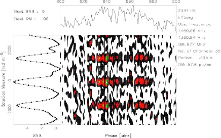
Figure 1: Illustration of the method used to determine pulsar RMs showing examples of PSRs J2113+4644 (left) and J2337+6151 (right). The top panel in each plot shows the total intensity of the pulsar. The central panel shows a contour plot of the S/N of the linear polarization as a function of assumed RM values (vertical axis) and pulse phase (horizontal axis). Pulse phases within the shown vertical lines have been collapsed to obtain the S/N as a function of RM that is displayed in the left panel.

Currently, about 1500 pulsars are known. While RMs are published only for about 350 of them, most of the major projects over the last decade were undertaken in the southern hemisphere (e.g. Han et al. 1999). Thus there remain a large number of pulsars for which RM are largely unknown. In order to augment the sample, in particular towards our selected region of the Perseus arm, we have undertaken a project of measuring RMs of pulsars using the 100-m Effelsberg radio telescope.

A sample of pulsars in the northern hemisphere ($\delta$ $>0^{\circ}$) for which no RM are available, was chosen from the Taylor, Manchester & Lyne (1993, updated version 1995) pulsar catalogue. Observations were made using the Effelsberg telescope in October/November 2001 using the 1.4 GHz HEMT receiver installed at the prime focus of the telescope. This receiver is tunable between 1.3 and 1.7 GHz. For median elevations the receiver has a noise temperature of 25 K. Dual circularly polarized signals, LHC and RHC, are mixed down to an intermediate frequency of 150 MHz and fed into the coherently de-dispersing Effelsberg Berkeley Pulsar Processor (EBPP, for technical details see Backer et al. 1997). Within the EBPP, the signal is split into four sub-bands using four down-converters. Each down-converter consists of two mixer filter modules (MFs) and one local oscillator (LO). Each MF receives two orthogonally polarized IF signals that are fed by the common LO, before they are passed into digital filter boards (DFBs). Each DFB provides a further sub-division of the signals into eight channels, which are then coherently de-dispersed in hardware by de-disperser boards (DBs). At the end a total of 32 channels for each polarization are obtained. Depending on the frequencies of the four LO’s the sub-bands can be spread across the available observable receiver bandpass in four sub-bands, symmetrically placed with respect to the centre frequency of observation. This option of the EBPP is quite useful for better RM estimates at 1.4 GHz where the sub-bands can be spread to obtain total bandpass of $\sim$100 MHz. The bandwidth of each final frequency channels depends on the DM of the observed pulsar, but is limited to 0.875 MHz for the polarization mode at around 1.4 GHz. In total, a bandwidth of 28 MHz is available, spread around in four sub-bands of 7 MHz. All signals are detected and folded in phase with the topocentric pulsar period. Each sub-integration which typically lasts for 180–300 s is transferred to a computer for offline processing.

Each observation of a pulsar to measure its RM is preceded by a calibration scan where the signal of a noise diode is injected into the waveguide following the feed horn. Pulsar and calibration scans are used to construct the pulsar’s Stokes parameters $I$, $Q$, $U$ and $V$ for each frequency channel. Parallactic angle corrections are applied to Stokes $U$ and $Q$ before all sub-integrations for a given pulsar are finally aligned in time and added to form the integrated Stokes parameters for all 32 frequency channels.

A search in rotation measure is performed by maximizing the linearly polarized intensity across the pulse phase. Stokes $U$ and $Q$ are appropriately rotated for a given value of the RM and then added for all the frequency channels to produce the linearly polarized intensity $L=\sqrt{U^{2}+Q^{2}}$. Phase bins across the pulse where the signal-to-noise ratio (S/N) of $L$ exceeds a threshold of 3 are collapsed to find the average S/N as a function of RM. The curve’s most significant peak with a S/N $>$5 is identified as being close to the pulsar’s RM. A finer search is then performed close to this peak to improve the RM estimate.

Since position angles are ambiguous by 180^∘, searches are performed for an increased RM range until a second peak in the S/N vs RM curve is obtained. The solution with the highest S/N can be clearly identified and is taken as the measured pulsar RM. Figure 1 gives two examples of the described technique for PSRs J2113+4644 and PSR J2337+6151. Although the S/N is very different, the RM can be accurately determined in both cases.

Uncertainties in the measured RMs are estimated directly from the S/N vs RM curves. The curves show a rather symmetric behaviour around the peak and positive and negative errors are determined by reading off the RM values corresponding to those values where the S/N decreases by one unit. Since 32 independent channels are used to produce these S/N curves, the resultant error is divided by $\sqrt{32}$. One way to check the validity of our method is to choose pulsars where in a given phase bin the S/N of $L$ of all the available frequency channels is significantly high ($>$ 10). In this case we can construct the position angle $\Phi=0.5{\rm tan}^{-1}(U/Q)$ and fit a straight line of the form $\Phi=\Phi_{\circ}+{\rm RM}\leavevmode\nobreak\ \lambda^{2}$, where $\lambda$ is the wavelength in meters. The resulting RMs and their formal errors obtained by this method are in good agreement with the procedure described above. For PSR J2113+4644 shown in Fig. 1, for instance, both methods yield a RM of 230$\pm$8, which is also in good agreement with the value available from the literature of 224$\pm$2. Other test pulsars with known rotation measures yield a similar good agreement with the earlier measurements.

We concentrated our measurements on pulsars located in a region within $85^{\circ}<l<245^{\circ}$ and $-10^{\circ}<b<10^{\circ}$. There are 56 known pulsars in this direction. Table 1 lists 44 of them for which RMs have been determined. Those pulsars with RM measurements obtained in this paper are highlighted by boldface in the table.

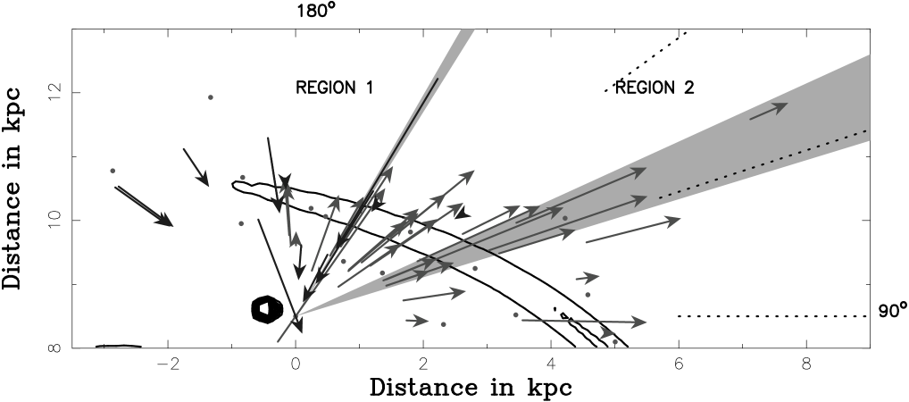
Figure 2: Distribution of pulsars in the Galaxy towards the Perseus arm within a Galactic latitude range of $-10^{\circ}<b<10^{\circ}$. The Sun is located at ordinate 8.5 kpc and abscissa 0 kpc. Pulsars with arrows directed towards the observer have positive RM and those away from the observer have negative RM. The size of the arrows are proportional to the $B_{\parallel}$ as calculated using Eqn. 1 with the pulsars located at the center of the arrows. The dots are pulsars for which RM values are not available.

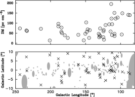
Figure 3: (Bottom) Distribution of HII regions as obtained from the Sharpless (1959) catalogue along the Galactic plane with longitudes $85^{\circ}<l<245^{\circ}$ and Galactic latitudes $-10^{\circ}<b<10^{\circ}$. Approximate sizes are depicted as gray ellipses using the angular extent as given by the catalogue. Note that detailed size and shape of the HII regions can be different from what is shown here. The positions of pulsars for which RM information is available are overlayed on the plot with crosses. (Top) Corresponding DMs observed for the pulsars shown.

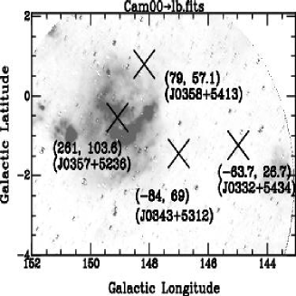
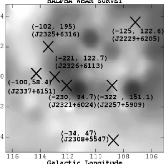
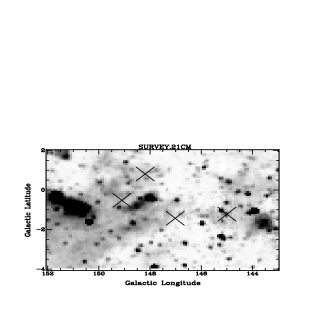
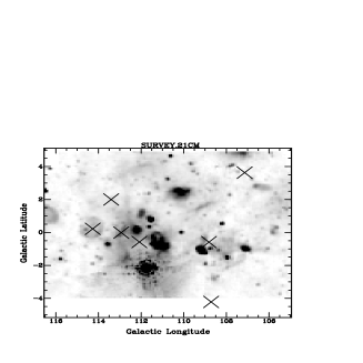
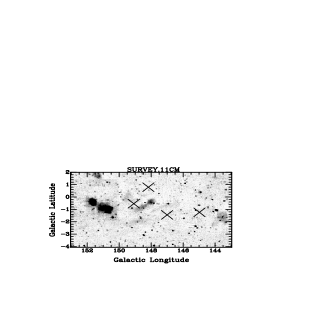
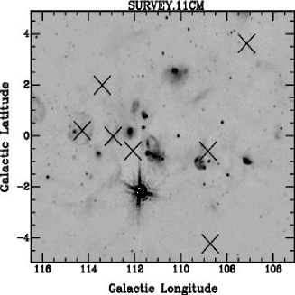
Figure 4: Pulsar positions overlayed on (left) Region 1 and (right) Region 2 as seen in several frequency ranges. The upper most panels shows an H$\alpha$ map, while the middle and bottom plots show radio continuum maps at $\lambda$21cm and $\lambda$11cm, respectively. The crosses in the figures indicates the position of the pulsars. The (RM,DM) and the pulsar name are indicated next to the crosses in the topmost figures of the right and left panel.

3 The Perseus Arm

Our aim is to study the effect of highly ionized HII regions on pulsar RMs. Noting that the distribution of HII regions peaks within a few degrees of the Galactic plane, we restrict the pulsars studied to $|b|<10^{\circ}$, i.e. ensuring that all pulsars lie within a height, $z$, above the Galactic plane of 1 kpc (see Table 1), which is also the typical electron density scale height. In Figure 2 we plot the top view of the Galaxy as given by the spiral arm model of Georgelin & Georgelin (1976) along with the distribution of pulsars that are located within our selected latitude range. Pulsar distances are estimated from the Cordes & Lazio (2002, CL02 hereafter) electron density model. The CL02 model is a significant improvement over the Taylor & Cordes (1993) electron density model as it takes into account the clumped structure of the ISM thus giving improved distance estimates to pulsars. Note that we also include PSR J0056+4756 in our study. With $b=-14^{\circ}$ it lies outside our nominal $|b|<10^{\circ}$ strip, but due to its small estimated distance, it has a small $z$-height of only $-0.26$ kpc.

The RM and DM of pulsars is used to estimate the average parallel component of the regular magnetic field as,

$$B_{\parallel}=1.232\leavevmode\nobreak\ {\rm(RM/DM)}\leavevmode\nobreak\ \leavevmode\nobreak\ \leavevmode\nobreak\ \mu{\rm G}$$ (1)

where RM is in rad m^-2 and DM in pc cm^-3. This estimate holds only if the variations of $B_{\parallel}$ and $n_{e}$ are uncorrelated along the line of sight (Beck 2001). As evident from Figure 2, near the solar neighbourhood there is a regular component of the magnetic field which changes sign due to the line of sight effect (Rand & Lyne 1994, Indrani & Deshpande 1997, Han et al. 1999, Frick et al. 2001).

In the bottom panel of Fig. 3 we plot the distribution of HII regions from the Sharpless (1959) catalogue that are located within $85^{\circ}<l<245^{\circ}$ and $|b|<10^{\circ}$, and along with the pulsars for which RMs are available. Among the 45 pulsars with measured RM, 14 of them have positive RMs. Around $l\sim 149^{\circ}$ there are two pulsars with high positive RM (cf. Fig. 2) which we refer to as Region 1 hereafter (see also Table 1). If the regular component of the magnetic field follows the Perseus arm, and the pulsars sample only the regular component of the magnetic field, then all the pulsars in this longitude range should have negative RMs. Thus the positive RMs could arise either due to reversal of the regular component of the magnetic field or due to some locally turbulent component of the field which disturbs the regular field sufficiently. Such turbulent components could also be responsible for anomalously high negative RMs.

In the top panel of Fig. 3, we plot the DM of those pulsars shown in the bottom panel. Apart from Region 1, a increase in both RM and DM of pulsars is seen around Galactic longitude of $l\sim 113^{\circ}$, which we call Region 2 hereafter (see also Tab. 1). Pulsars in Region 1 and Region 2 have lines-of-sight either directly through or close to HII regions. RM of pulsars behind these regions are thus susceptable to be affected seriously by these HII regions. We investigate this issue further below.

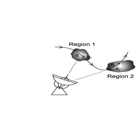
Figure 5: Schematic model of the magnetic field in the direction of the Perseus arm. See text for details.

Figure 6: Variation of the estimated $B_{\parallel}$ with Galactic longitude. The dashed line is a linear fit to the data and the solid triangles are the fit by using the model described in section. 4. The open circles are the observed $B_{\parallel}$ for the selected pulsars.

Figure 7: Left:Variation of RM versus DM of pulsars lying within three Galactic longitude range are shown. The open circles are pulsars which lie behind HII regions and supernova remnants. The filled circles are pulsars which are apparently not affected by HII regions along the line of sight. The dashed line is the straight line fit to data points. The $B_{\parallel}$ obtained from the fits are shown in the figure. Right: Variation of RM with distances are shown for the three different sections. The symbols are same as that in the left panels. See text for further details.

Figure 8: In the above plot the residuals of RM’s and $\sigma_{\rm rm}$ are plotted as a function of distance to the pulsar. The residuals of RM are denoted by open circles, and the estimated $\sigma_{\rm rm}$ are denoted by filled squares. The dashed line corresponds to $40\sqrt{D}$. See text for further detail.

3.1 Region 1: $l=149^{\circ}$

In this region data are available for four pulsars and three extra-galactic sources. The pulsars J0357+5236 and J0358+5413 have positive RMs while the nearby objects PSRs J0332+5434 and J0343+5312 have negative RMs. Three EG sources in this area (Kronberg, private communication) also have negative RMs. The DM of PSR J0357+5236 is particularly high, much higher than for all other nearby pulsars. We have overlaid the position of the four pulsars on a H$\alpha$ image taken from the Virginia Tech Spectral-Line Survey (VTSS, Simonetti et al. 1996) in Fig. 4. It shows that PSR J0357+5236 is seen directly towards a bright HII region, explaining the high DM of the object. The change in sign pertains to two pulsars, both seen through the bright HII region. The DM of the other pulsars is similar suggesting them to be close to each other. There are two more observables givng evidence of dense ionized HII region towards a pulsar. Firstly it is expected that electron density fluctuation in strongly ionized HII regions will result in scatter broadening of pulsar signals (see Mitra & Ramachandran 2001 and references therein). Secondly the emission measures towards these directions should be significantly higher. While the pulse shape of PSR J0357+5236 shows an apparent signature of scatter broadening in the form of an conventional exponential decay of the pulse profile, we are not aware of any measurements available for this pulsar in the literature. In fact no conclusion can be drawn regarding this without any detailed analysis as scattering measurements are influenced strongly by the intrinsic pulse shape (Löhmer et. al. 2001). The scatter broadening time for J0358+5413 is 2.3$\times 10^{-4}$ msec, almost 4 times higher than the nearby pulsar J0332+5434 (refer pulsar catalogue Taylor, Manchester & Lyne, 1993). The emission measures towards PSR J0357+5236 and J0358+5413 are about 103 and 29 pc cm^-6 compared to an average value of 10 pc cm^-6 towards the nearby objects (data from Müller et. al. 2003, private communication). These evidences further reinforces the conclusion that PSR J0357+5236 and J0358+5413 are potentially behind the HII region S205.

Overlaying the pulsar positions onto $\lambda$21cm and $\lambda$11cm radio continuum maps (Reich et al. 1990, Fürst et al. 1990) in Fig. 4, we notice that the pulsars are seen through complex Galactic emission regions. The fact that at $\lambda$11cm the diffuse emission is less than at $\lambda$21cm suggests the presence of strong non-thermal emission in this direction.

A large region near $l\sim 145^{\circ}$ is occupied by the Camelopardalis dark clouds which are amongst the closest dust formations in the solar vicinity (Zdanavicius et al. 2001). The HII region S205 (Sharpless 1959) which is of interest has its northern half in the Camelopardalis and the southern half in the Perseus constellation. S205 is thought to be ionized by the O8 star HD 24451 and is also listed in the catalogue of bright nebula by Lynds (1965). Using the CO velocities of the optical HII emission, Fich & Blitz (1984) quote a distance for S205 of 900$\pm$300 pc. Using the angular diameter of the optical HII region, they also obtain a linear size of 31.4$\pm$10.5 pc.

Having identified PSRs J0357+5236 and J0358+5413 to be lying behind S205, these pulsars can now be used to put constrains on $n_{e}$ and $B_{\parallel}$ for this HII region. Apart from these two pulsars the other objects in the nearby region have an average DM of $\sim$ 50 pc cm^-3. If we attribute the increased DM of 103.65 pc cm^-3 for PSR J0357+5236 entirely to S205, then the excess DM is $\sim$53 pc cm^-3. Further we can use S205’s transversal scale of 30 pc to estimate $n_{e}$ to be 1.8 cm^-3. The average RM of the nearby pulsars is $\sim-50$. With the estimated $n_{e}$ = 1.8 cm^-3 over a distance of 30 pc, we infer $B_{\parallel}\sim 5.7\mu$G which is sufficient to explain PSR J0357+5236’s increased RM of 261. To explain the lower RM and DM values of PSR J0358+5413 a nominal value of only $n_{e}\sim 0.75$ cm^-3 would be sufficient while keeping $B_{\parallel}$ constant. Of course, apart from this simple model, another way to explain the increased DM and RM values would be to incorporate variations in both $n_{e}$ and $B_{\parallel}$. This however would require the HII region to modulate the magnetic field within itself which is of the order of several $\mu$G. Albeit such strong magnetic fields might not be easy to generate in HII regions. Thus it is possible that S205 is associated with a local loop of the magnetic field where the field twists in the direction of the observer while the magnetic field strength across the 30 pc scale estimated for S205 is rather constant.

3.2 Region 2: $l=113^{\circ}$

The other region of RM variation is seen around $l\sim 113^{\circ}$. There are 7 pulsars in this direction which are listed in Tab. 1. In the right hand top panel of Fig. 4 we have overlayed the pulsar position on the H$\alpha$ map observed by the Wisconsin H$\alpha$ mapper (WHAM, Haffner et al. 2001). Apparently, PSRs J2229+6205, J2308+5547, and J2325+6313 are in regions free from enhanced emission. The estimated average $B_{\parallel}$ for these pulsars is about 1$\mu$G. From the low DM of 47 pc cm^-3 for J2308+5547 the estimated model distance is 2.2 kpc. The other two objects PSRs J2229+6205 and J2325+6313 have high DMs of 122.6 and 195 pc cm^-3 which correspond to distances of 4 and 8 kpc, respectively. The nearly constant estimated $B_{\parallel}$ for these two pulsars suggests that the magnitude of the regular component of the magnetic field is constant over a large distance beyond the Perseus arm (see Tab. 1).

The pulsars J2257+5909, J2321+6024 and J2326+6113 are seen to lie towards a complex of enhanced H$\alpha$ emission (Fig. 3 and  4). The increase in DM for these objects is also associated with an increase of RM giving an average $B_{\parallel}$ of 2.6$\mu$G. PSR J2337+6151 is known to be associated with the supernova remnant G114.3+0.3 (Kulkarni et al. 1993, Fürst et al. 1993) and is prone to have an anomalous RM behaviour. In fact, the estimated $B_{\parallel}$ of 2.1$\mu$G is higher than the regular component in the Perseus arm. This also supports the fact that the pulsar is associated with the supernova remnant.

The overlays of these pulsars on the radio continuum total intensity maps of $\lambda$21cm and $\lambda$11cm are shown in Fig. 4 (Reich et. al. 1990, Fürst et. al. 1990). The fading of several structures between these two frequencies shows the non-thermal behaviour of these regions while there are some complexes which seem to remain thermal. Another possibility for this apparent fading might that the emission is too faint to be detected in usually less sensitive high-frequency radio surveys. Unlike Region 1, this area is far more complex in terms of distribution of HII regions. paper.

For PSR J2257+5909 a number of HII regions may contribute to the enhanced electron density along the path, i.e. S152, BFS14 and/or BFS15 (Blitz et al. 1982). The distance estimated from CO velocities for S152, which is closest to the pulsar, is 3.6$\pm$1.1 kpc. The estimated CL02 model distance to the pulsar is 4.5 kpc, thus placing the pulsar behind the HII regions.

PSRs J2321+6024 and J2326+6113 lie close to the HII regions S161A, S161B, S162 and S163. S161A and S161B are considered to be two HII regions almost superposed on each other with a distance of 2.8$\pm$0.9 kpc (Blitz et. al. 1982). With S162’s distance estimate of 3.5$\pm$1.1 kpc, all three regions are close to PSR J2321+6024 whose distance using the CL02 model is $\sim$3 kpc. S163 has a distance of 2.3$\pm$0.7 kpc and is closer to PSR J2326+6113 whose model distance is 4.5 kpc, again indicating that the pulsar is behind the HII region. Note that within the uncertainties all HII regions are located at a distance of approximately 3 kpc. Again, it seems likely that the HII complexes are associated with a local loop of the magnetic field, but now the direction of the field is directed away from the observer. The situation of both Region 1 and Region 2 is illustrated schematically in Fig. 5.

It should be noted that although while estimating distances to pulsars the CL02 model tries to take into account the enhanced electron density due to HII regions for specific lines of sight these distances might still be inaccurate. However, without complete knowledge about the length scales and the $n_{e}$ of these HII regions, it is not possible to calculate these distances accurately.

4 The regular component of the magnetic field

Our investigation has concentrated on a region of $85^{\circ}<l<245^{\circ}$ and $|b|<10^{\circ}$. In order to study the large scale configuration of the regular Galactic magnetic field towards the Perseus arm, we now consider all pulsars in this region, summarized in Table 1. Having shown that anomalous variations of RM and DM can be associated with HII regions, in particular in our so-called Regions 1 and 2, we are now in the position to use Table 1 to construct a sample of sources that is free from such misleading effects.

The sample listed in Table 1 includes a few pulsars which are believed to be associated with supernova remnants. PSRs J0502+4654 and PSR J0538+2817 are located within the boundaries of the supernova remnants G160.9+2.6 (HB9) and G180.0$-$1.7 (S147), respectively. From surface brightness-diameter relations (e.g. Milne 1979) the distance to G160.9+2.6 is thought to be $\sim$1.2 kpc (Leahy & Roger 1991) which is in good agreement with the distance of $\sim$1.4 kpc to PSR J0502+4654 estimated from the CL02 model, suggesting a physical association of the pulsar with the supernova remnant. PSR J0538+2817 has a distance of $\sim$1.2 kpc and is thought to be physically associated with the G180.0$-$1.7 whose distance is estimated to be $\sim$0.8 kpc as deduced from interstellar redenning measurements ( Fesen et al. 1985, see also Anderson et al. 1996) and $\sim$1.6 kpc based on surface-brightness diameter relationship (Sofue et al. 1980). As pointed out before, it is uncertain about how a supernova remnant affects the RM of such pulsars, and thus we exclude these objects from further discussions. For similar reasons, we do not consider the Crab pulsar, PSR J0534+220.

The remaining 36 pulsars form a carefully selected sample with RM and DM values that are free from any obvious anomalies that might be introduced due to bright HII regions or supernova remnants. For all these pulsars, labeled with a ‘G’ in Table. 1, we use Eqn. (1) to compute the weighted average of $B_{\parallel}$, and we plot the resulting values as a function of Galactic longitude in Figure 6.

Inspecting Fig. 6, there is some tendency for the average $B_{\parallel}$ to decrease from $l\sim 90^{\circ}$ to $l\sim 150^{\circ}$. Beyond $l\sim 150^{\circ}$, we notice an increase in mean B_∥ from negative to positive values. In the simplest model, the distribution of points in Fig. 6 could be described by fitting a linear dependence to the data as shown by the dashed line. Since the estimated uncertainties in the average $B_{\parallel}$ are much smaller than the spread in the data points, however, an unweighted least-squares fit was performed to derive the shown linear dependence which is clearly only a crude description of the data.

In order to forge a better understanding, we can instead try to test whether the data are result of the magnetic field following the local Perseus arm. The motivation for this comes from examples of external galaxies, where the large scale inter-arm field seems to trace the optical spiral arms with a slight phase offset (Beck 2001). We consider a model where the regular uniform magnetic field of magnitude $B_{\rm o}$ traces the spiral arm as depicted by Georgelin & Georgelin (1976). In our model this field is meant to be located not only on the spiral arm, but also in the inter-arm regions between the solar system and the Perseus arm as well as beyond the arm. We use the procedure of cubic spline fit as adopted by Taylor & Cordes (1993) to construct the spiral arm and the direction of the field lines. The angle between the field lines and the line of sight varies with distance and Galactic longitude so that varying amounts of the global field will be projected onto the line of sight when a radiowave travels from the pulsar to solar system. To account for that effect we integrated numerically over the projected B_o along the line of sight for every source to obtain their effective $B_{\parallel}$. This dependence of $B_{\parallel}$ is then used to fit the data points. In addition we allow for another free parameter to be determined, i.e. $\theta$ which describes the possibility that the so-called ‘magnetic arm’ might actually be at a phase offset with respect to the spiral arm, a circumstance which is also commonly observed in external galaxies (Beck 2001). A positive value of $\theta$ means that the spiral arm needs to be rotated around the Galactic Centre in the counter-clockwise direction by that amount to fit the ‘magnetic arm’ along which the regular component of the field reside. A least-square fit to the data gives $\@vec{B_{\rm o}}$ as 1.7$\pm$1.0 $\mu$G and $\theta=12^{\circ}\pm 8^{\circ}$ as shown by the solid triangles in Fig. 6. There has been several previous attempts to estimate $B_{\rm o}$. For example Rand & Kulkarni (1989) and Lyne & Smith (1989) estimated $B_{\rm o}\sim 1.5\mu$G. More recently Han & Qiao (1994) and Indrani & Deshpande (1998) estimated $B_{\rm o}\sim 1.8\mu$G. Our value of $B_{\rm o}$ is consistent with all the previous estimates.

While the significance is not very high, the positive value of $\theta=12^{\circ}\pm 8^{\circ}$ may indeed indicate that ‘magnetic arm’ is at some angle to the spiral arm. In fact we can now use our model to find the pitch angle of the ‘magnetic arm’ which we define as the angle between the tangent to the arm and the tangent to the logarithmic spiral in the direction $l=180^{\circ}$. The model of the Perseus arm by Georgelin & Georgelin (1976) gives a pitch angle of $\sim-19^{\circ}$ while our phase offset model considered above gives a pitch angle for the ‘magnetic arm’ of $-10^{\circ}\pm 8^{\circ}$, which is in good agreement with the earlier estimate of $-8^{\circ}$ (e.g. Han et al. 1999, Indrani & Deshpande 1998). However, a larger data set and an analysis extending to a larger longitude range is obviously essential to discern this effect with more sophisticated models than applied here as a first approach.

Indeed, the model of the regular field considered here is, almost certainly, far too simple. It is quite likely that the magnetic field amplitude changes as a function of pulsar distance, a situation which was considered in detail by Rand & Lyne (1994). A crude way to investigate this is to study the variation of pulsar RM with distance. For a uniform magnetic field and constant $n_{e}$, we expect a linear increase of RM with distance. Assuming that no sign reversals are present, any significant deviation would, in contrast, point to changes in magnetic field amplitude or $n_{e}$. However, we are confident that the distribution of $n_{e}$ along the line-of-sight to pulsars in our selected sample is relatively uniform, so that we can attempt this exercise for the magnetic field. In order to avoid problems caused by possible uncertainties in the distance model, we study three separate sections, i.e.  $85^{\circ}<l<130^{\circ}$, $130^{\circ}<l<180^{\circ}$ and $180^{\circ}<l<245^{\circ}$, respectively. In all cases, the data are consistent with a constant magnetic field amplitude. We show the RM versus DM dependence for all the $l$ range in Fig. 7. The slope in the figures are proportional to the $B_{\parallel}$ but no significant change in slope is evident. However the spread of the data points increases noticeably with DM, an effect which we discuss further below.

The formal uncertainty of our determined $B_{\circ}$ value is 1$\mu$G which is also visible from Figure 6. This is much larger than the relative error of the fitted $B_{\parallel}$ values which is typically about 5 to 10% and dominated by the uncertainties in RM. We can understand this discrepancy by considering that our model does not take into account any possible small-scale fluctuations of the magnetic field in strength and direction which may be correlated with the local electron density (Beck 2001).

It is possible that many more HII regions, too faint to be detected by current surveys, are associated with the random component of the magnetic field. Sokoloff et. al. (1998) and Gaensler et al (2001) studied various effects and could relate the fluctuation of RM’s, $\sigma_{\rm{}_{rm}}$, as

$$\sigma_{\rm{}_{rm}}=0.81\times\delta n_{e}B_{r}\sqrt{L_{r}D}\leavevmode\nobreak\ \leavevmode\nobreak\ \leavevmode\nobreak\ \rm{rad\leavevmode\nobreak\ m^{-2}}$$ (2)

where $\delta n_{e}$ is the fluctuation of the electron density in cm^-3 and $B_{r}$ in $\mu$G the random component of the magnetic field towards the pulsar. While $D$ is the distance to the pulsar measured in pc, $L_{r}$ (in pc) is the length scale over which $B_{r}$ fluctuates. For a determination of the involved parameters, Rand & Kulkarni (1989) studied pulsars with small angular and linear separations. They introduced a model where they divided the distance to each pulsar into a number of single cells of constant length $L_{r}$ with randomly oriented field components of strength $B_{r}$. As a result, they found a length scale of $L_{r}\sim$50 pc and random magnetic field of $B_{r}\sim$ 5$\mu$G. This small value of $L_{r}$ can be compared to values of 100 pc and 1000 pc, respectively, which Rand & Kulkarni (1989) inferred for the North Polar Spur and an area which they called “Region A” where they found the magnetic field to be highly organized.

Interestingly, we can use the data obtained for our Region 1 to obtain another, independent estimate for the parameters. Here we can infer the excess in electron density $\delta n_{e}$ from the increased DM and the observed transverse length scale of about $L_{r}\sim$30 pc as mentioned in Section 3. Further using the increased RM and the estimated $\delta n_{e}$ and $L_{r}$, we obtain a value of $B_{r}\sim$ 5.7$\mu$G. Both $L_{r}$ and $B_{r}$ estimated for Region 1 are in good agreement with the estimates of Rand & Kulkarni (1989) as mentioned above. Thus, we can demonstrate here that pulsars lying behind HII regions can be used as probe to find the local turbulent random component of the magnetic field $B_{r}$.

Based on our model for the regular component of the magnetic field, we can estimate the value of $\sigma_{\rm{}_{rm}}$ by using the post-fit residuals $\mid B_{\parallel}-B_{\rm model}\mid$, obtained after applying our magnetic field model to the data (solid line in Fig. 6). These residuals are converted to residuals in RM using Eqn. 1. In Fig. 8 the open circles show the residual of RM’s as a function of the CL02 model distance. To find $\sigma_{\rm{}_{rm}}$ we consider distance intervals of 1 kpc. For each such bin we equate $\sigma_{\rm{}_{rm}}$ to the square root of the mean of the squares of the RM residuals. The filled squares in Fig. 8 show the estimated $\sigma_{\rm{}_{rm}}$ placed at the centre of the distance bins considered. The estimated error bars reflects the number of points available in each bin. We have not used PSR J2325+6316 which is at a distance of $\sim$8 kpc as there is only one pulsar in that distance bin. The increase in $\sigma_{\rm{}_{rm}}$ with DM (or distance) seen here is consistent with the aforementioned increasing scatter in the RM-DM plot of Fig. 7.

The dashed line shown in Fig. 8 corresponds to $40\times D^{0.5}$. We show this line only for illustration to compare the data to a $\sqrt{D}$-dependence which is expected from Eqn. 2 if the parameters $\delta n_{e}$, $B_{r}$ and $L_{r}$ are distance independent. While the data are not adequate to claim such a $\sqrt{D}$-dependence, we can certainly see that $\sigma_{\rm{}_{rm}}$ increases with distance.

5 Field reversals revisited

Several previous studies have argued for field reversals in the Perseus arm and beyond based on specific behaviour of the RM distribution of pulsars and EG point sources (Lyne & Smith 1989, Clegg et al. 1992, Han et al. 1999, 2002). A lucid description of the various reasons leading to conclusions regarding field reversals can be found in Han et al. (1999). Culmination of all these studies leads to the proposal that a field reversal on Galactic scale is observed beyond the Perseus arm. While the large scale magnetic field is seen to follow a clockwise direction between the Perseus and the Carina-Sagittarius arm, it is argued that the magnetic field beyond the Perseus arm follow a counterclockwise direction.

The paucity of pulsars beyond a distance of $\sim$6 kpc forces us to rely only on the RM’s of EG sources to study the magnetic field beyond the Perseus arm. As discussed in Brown (2002) and clarified further in Brown et al. (2003; in preparation) one needs EG sources which are confined to a narrow latitude range. Here we revisit the question of field reversal towards the Galactic longitude range of $85^{\circ}<$ l $<240^{\circ}$ based on our findings of anomalous RM of pulsars in Region 1 and 2. In Fig. 7 we show the behaviour of RM with DM (left panels) and RM with CL02 model distances D (right panels) to pulsars in three specific longitude ranges. The pulsars affected by the HII regions and supernova remnants are indicated by open circles in the figure. If the pulsars with open circles are excluded, then the RM of the filled points are seen to show an overall mean increase with DM as shown by the dashed line in the figure, with no significant change in slope with DM (or D). The slope is proportional to the average $B_{\parallel}$ component and no noticeable change in $B_{\parallel}$ upto a distance of 5–6 kpc is observed. While the spread in the RM is seen to increase with both DM and D in the shape of a cone as expected from Eqn. 2. Thus the data seems to be consistent with a constant magnetic field upto a distance of 5–6 kpc towards the Persues arm. We can compare to this to the results by Han et al. (1999) who suggested a large scale field reversal in our Region 2 at about 5–7 kpc. The conclusion for this particular region was based on the observation that the RMs of pulsars and EG sources beyond this distance seemed to become less negative which can also be seen in the uppermost left panel of Fig. 7. While their is considerable scatter in the EG sources, we have shown that RM of the pulsars in this regions are affected by HII regions. The argument for the suggested field reversal is hence weakened. Also for Region 1 we have shown that the positive contribution of the RM arises from the HII region which further weakens the hypothesis of the reversed field as was suggested by Han et al. (1999).

Considering the electron density scale height to be 1 kpc, only sources that lie within $|b|\pm 10^{\circ}$ will sample the magnetic field for a distance larger than 6 kpc. However, not many RM measurements are currently available for such low latitudes. In the past, Lyne & Smith (1989) used 19 EG sources lying within $|b|\pm 30^{\circ}$ from the Simard-Normandin & Kronberg (1980) catalogue and noted that the mean RM for these sources were notably smaller than that of the distant pulsars and considered this to be indicative of field reversal in the outer Galaxy. However there are only 5 EG sources which lie within $|b|\pm 10^{\circ}$, so that their conclusion and also that of Han et al. (1999) for Region 2 might have been influenced by inadequate statistics.

The ongoing Canadian Galactic Plane Survey (CGPS , Landecker et al 2000) is an effort towards augmenting RM statistics for EG sources (Brown & Taylor 2001) which should improve our understanding of the magnetic field in the outer Galaxy significantly. As mentioned earlier that their initial results already suggest RM values of $\sim\pm$ 400 within $|b|\leq 4^{\circ}$. Further the effect of HII regions also needs to be taken into account for such a study.

6 Discussion and Conclusion

In this paper we investigated the effect of HII regions on observed pulsar RMs, isolating the region in the direction of the Perseus arm between Galactic longitude $85^{\circ}<l<245^{\circ}$ and Galactic latitude $|b|<10^{\circ}$ for our study. We find that there are two regions as discussed in Section 4 where RM and DM of pulsars increases anomalously due to presence of small scale HII regions along the line-of-sight. We present a comparative study of these regions seeking evidence from H$\alpha$ maps and further following the nature of the emission as evident from $\lambda$21cm and $\lambda$11cm radio continuum. For Region 1 there are two pulsars which are strongly affected due to presence of the HII region S205. Based on the pulsars’ RM and DM estimates we conclude that the increased RM observed in the centre of S205 can be well explained by an increase in electron density within this region. Interestingly, this region seems to be associated with a region where locally the magnetic field is directed towards the observer as illustrated in Fig. 5. For Regions 2 we find 4 pulsars to be lying behind HII complexes which explains an observed RM and DM anomaly. Demonstrating how the presence of HII regions strongly affects the RM of pulsars, we emphasize the need for a carefully selected sample of pulsars that is unaffected by line-of-sight effects when studying the regular large scale component of the magnetic field.

In earlier studies of the Galactic magnetic field the effect of large supernova remnant like the North polar spur and the Gum Nebula has been taken into account (Rand & Kulkarni 1989, Indrani & Deshpande 1998). This region spans a large angular scale in the sky and thus the pulsars behind these regions are excluded for the analysis of large scale magnetic field supposing that these region introduce RM anomalies. Given the limited number of pulsars available for any statistical analysis, however it is not entirely reasonable to reject all pulsars behind large HII complexes. This is also true as the HII regions are clumpy and the pulsars might be located in regions where the RM is relatively unaffected by the HII regions. Such information can only be obtained by careful study of H$\alpha$ and radio continuum emission as we have shown in this paper. A lack of such analysis might lead to several controversial conclusions. For demonstration, we revisited Han et al. (1999)’s argument that the RM’s in direction of $l\sim 113^{\circ}$ (our Region 2) give indications for a field reversal on Galactic scales at a distance of 5–7 kpc. As we have shown, this region is strongly influenced by the presence of ionized HII complexes. While the paucity of distant pulsars prevents drawing firm conclusions for beyond the Perseus arm, our analysis excludes a reversal of magnetic field towards $85^{\circ}<l<245^{\circ}$ for distances of less than 5–6 kpc. As mentioned before Indrani & Deshpande (1998) in their analysis employed a selection criteria where they excluded all pulsars which has $B_{\parallel}>3\mu$G. We however note that in our sample all the pulsars affected by HII region have $B_{\parallel}<3\mu$G (see Tab. 1), and thus would not have been excluded in their analysis.

Further evidence of RM of extra-galactic sources being affected by HII regions have been noted by Brown & Taylor (2001) in the region $l=92^{\circ}$ and $b=0.5^{\circ}$. In the recent CGPS the RM of about 380 sources are determined (Brown & Taylor 2001). All these sources lie in the $|b|<4^{\circ}$ of the Galactic plane. This is in contrast to the data of Simard-Normandin & Kronberg (1980) who had data on sources away from the Galactic plane. In particular in the region $l=92^{\circ}$ and $b=0.5^{\circ}$, Brown & Taylor (2001) notes that most of the extra-galactic sources have negative RM’s. The few pulsars with determined RM have values less than the nearby extra-galactic sources. In three directions a sudden reversal of the sign of RM is seen. These regions are towards diffuse continuum emission, presumably HII regions. Based on this observation Brown & Taylor concluded that the magnetic field reversal correlates with nearby Galactic emission structures and not reversals on larger scales in the Galactic spiral arms. This conclusion is supported by our studies of Regions 1 and 2. Although comparison with H$\alpha$ data for these anomalous regions are essential, as sometimes the thermal HII is not visible in the continuum radio emission, either due to poor sensitivity or due to presence of non-thermal emission. This effect is clearly seen for Region 1 and Region 2 in Fig. 4.

In summary, we have presented several arguments demonstrating that HII regions strongly affect the RMs of pulsars. We have obtained 11 new RM of pulsars towards the Perseus arm which gives improved statistics to study the Galactic magnetic field in this direction. Using these new as well as previously published data we find 36 pulsars out of 45 available in the region of investigation which are unaffected by the presence of prominent HII regions. This careful selection helps to study the regular component of the magnetic field $B_{\parallel}$ in the Galactic disk Section 4. We derive the following conclusions.

a) The regular large scale component of the magnetic field has a magnitude of $1.7\pm 1.0\mu$G. The magnetic field follows the local Perseus arm rather well between $150^{\circ}<l<245^{\circ}$. There is significant deviation observed beyond l$\sim 150^{\circ}$. This deviation can be explained by considering the ‘magnetic arm’ to be at an angle of 12${}^{\circ}\pm 8^{\circ}$ with respect to the spiral arm or a pitch angle of $-10^{\circ}\pm 8^{\circ}$.

b) We find the fluctuation in RM to increase as a function of distance to the pulsar.

c) We do not find any evidence for a large-scale reversal of the Galactic magnetic field in direction of the Perseus arm at $85^{\circ}<l<245^{\circ}$ upto a distance of 5–6 kpc.

Table 1: Pulsars included in this study. We list the pulsar name, its Galactic longitude and latitude, dispersion measure, rotation measure and the distance and z-height as derived from the CL02 (2002) model. We also quote the magnetic field $B_{\parallel}$ as estimated from Eqn. 1 (last column). Pulsars with new RM measurements reported in this paper are highlighted in boldface. The DMs and RMs of pulsars marked with a G are unlikely to be strongly affected by HII regions (see text for further details).

Pulsar $l$ $b$ DM RM $D_{CL}$ $z$ $B_{\parallel}$ J2000 (deg) (deg) (pc cm^-3) (rad m^-2) (kpc) (kpc) ($\mu$G) Region 1 0332+5434_G 145.00 $-$1.22 26.776$\leavevmode\nobreak\ \pm\leavevmode\nobreak\$ 0.005 $-$63.7$\leavevmode\nobreak\ \pm\leavevmode\nobreak\$ 0.4 0.98 $-$0.02 $-$2.93$\leavevmode\nobreak\ \pm\leavevmode\nobreak\$ 0.02 0343+5312_G 147.0 $-$1.43 69$\leavevmode\nobreak\ \pm\leavevmode\nobreak\$ 2 $-$84$\leavevmode\nobreak\ \pm\leavevmode\nobreak\$ 20 2.05 $-$0.05 $-$1.5$\leavevmode\nobreak\ \pm\leavevmode\nobreak\$ 0.5 0357+5236 149.10 $-$0.52 103.650$\leavevmode\nobreak\ \pm\leavevmode\nobreak\$ 0.012 261$\leavevmode\nobreak\ \pm\leavevmode\nobreak\$ 13 2.78 $-$0.03 3.10$\leavevmode\nobreak\ \pm\leavevmode\nobreak\$ 0.2 0358+5413 148.19 0.81 57.14$\leavevmode\nobreak\ \pm\leavevmode\nobreak\$ 0.06 79$\leavevmode\nobreak\ \pm\leavevmode\nobreak\$ 4 1.45 0.02 1.70$\leavevmode\nobreak\ \pm\leavevmode\nobreak\$ 0.1 Region 2 2229+6205_G 107.15 3.64 122.6$\leavevmode\nobreak\ \pm\leavevmode\nobreak\$ 0.4 $-$125$\leavevmode\nobreak\ \pm\leavevmode\nobreak\$ 22 3.96 0.25 $-$1.2$\leavevmode\nobreak\ \pm\leavevmode\nobreak\$ 0.3 2257+5909 108.83 $-$0.57 151.070$\leavevmode\nobreak\ \pm\leavevmode\nobreak\$ 0.012 $-$322$\leavevmode\nobreak\ \pm\leavevmode\nobreak\$ 11 4.50 $-$0.04 $-$2.63$\leavevmode\nobreak\ \pm\leavevmode\nobreak\$ 0.1 2308+5547_G 108.73 $-$4.21 47.0$\leavevmode\nobreak\ \pm\leavevmode\nobreak\$ 0.4 $-$34$\leavevmode\nobreak\ \pm\leavevmode\nobreak\$ 3 2.17 $-$0.16 $-$0.89$\leavevmode\nobreak\ \pm\leavevmode\nobreak\$ 0.1 2321+6024 112.09 $-$0.57 94.78$\leavevmode\nobreak\ \pm\leavevmode\nobreak\$ 0.11 $-$230$\leavevmode\nobreak\ \pm\leavevmode\nobreak\$ 10 3.03 $-$0.03 $-$2.99$\leavevmode\nobreak\ \pm\leavevmode\nobreak\$ 0.1 2325+6316_G 113.42 2.01 195$\leavevmode\nobreak\ \pm\leavevmode\nobreak\$ 5 $-$102$\leavevmode\nobreak\ \pm\leavevmode\nobreak\$ 14 8.08 0.28 $-$0.64$\leavevmode\nobreak\ \pm\leavevmode\nobreak\$ 0.1 2326+6113 112.95 0.00 122.69$\leavevmode\nobreak\ \pm\leavevmode\nobreak\$ 0.02 $-$221$\leavevmode\nobreak\ \pm\leavevmode\nobreak\$ 10 4.86 0.0 $-$2.22$\leavevmode\nobreak\ \pm\leavevmode\nobreak\$ 0.1 2337+6151 114.28 0.23 58.38$\leavevmode\nobreak\ \pm\leavevmode\nobreak\$ 0.09 $-$100$\leavevmode\nobreak\ \pm\leavevmode\nobreak\$ 18 3.15 0.01 $-$2.1$\leavevmode\nobreak\ \pm\leavevmode\nobreak\$ 0.3 Others 0040+5716_G 121.45 $-$5.57 90.6$\leavevmode\nobreak\ \pm\leavevmode\nobreak\$ 0.5 9$\leavevmode\nobreak\ \pm\leavevmode\nobreak\$ 13 2.98 $-$0.29 0.12$\leavevmode\nobreak\ \pm\leavevmode\nobreak\$ 0.2 0056+4756_G 123.79 $-$14.92 18$\leavevmode\nobreak\ \pm\leavevmode\nobreak\$ 2 $-$23$\leavevmode\nobreak\ \pm\leavevmode\nobreak\$ 22 1.03 $-$0.26 $-$1.6$\leavevmode\nobreak\ \pm\leavevmode\nobreak\$ 1.5 0102+6537_G 124.08 2.77 65.84$\leavevmode\nobreak\ \pm\leavevmode\nobreak\$ 0.13 $-$94$\leavevmode\nobreak\ \pm\leavevmode\nobreak\$ 15 2.29 0.11 $-$1.8$\leavevmode\nobreak\ \pm\leavevmode\nobreak\$ 0.2 0108+6905_G 124.46 6.28 59.5$\leavevmode\nobreak\ \pm\leavevmode\nobreak\$ 0.6 $-$46$\leavevmode\nobreak\ \pm\leavevmode\nobreak\$ 19 2.22 0.24 $-$0.9$\leavevmode\nobreak\ \pm\leavevmode\nobreak\$ 0.4 0108+6608_G 124.65 3.33 30.15$\leavevmode\nobreak\ \pm\leavevmode\nobreak\$ 0.10 $-$29$\leavevmode\nobreak\ \pm\leavevmode\nobreak\$ 3 1.40 0.08 $-$1.19$\leavevmode\nobreak\ \pm\leavevmode\nobreak\$ 0.1 0139+5814_G 129.22 $-$4.04 73.75$\leavevmode\nobreak\ \pm\leavevmode\nobreak\$ 0.10 $-$90$\leavevmode\nobreak\ \pm\leavevmode\nobreak\$ 4 2.87 $-$0.2 $-$1.50$\leavevmode\nobreak\ \pm\leavevmode\nobreak\$ 0.1 0141+6009_G 129.15 $-$2.11 34.80$\leavevmode\nobreak\ \pm\leavevmode\nobreak\$ 0.10 $-$48$\leavevmode\nobreak\ \pm\leavevmode\nobreak\$ 3 2.18 $-$0.08 $-$1.70$\leavevmode\nobreak\ \pm\leavevmode\nobreak\$ 0.1 0147+5922_G 130.06 $-$2.72 40.10$\leavevmode\nobreak\ \pm\leavevmode\nobreak\$ 0.01 $-$19$\leavevmode\nobreak\ \pm\leavevmode\nobreak\$ 5 2.22 $-$0.10 $-$0.58$\leavevmode\nobreak\ \pm\leavevmode\nobreak\$ 0.2 0157+6212_G 130.59 0.33 29.8$\leavevmode\nobreak\ \pm\leavevmode\nobreak\$ 0.3 $-$29$\leavevmode\nobreak\ \pm\leavevmode\nobreak\$ 7 1.68 0.01 $-$1.20$\leavevmode\nobreak\ \pm\leavevmode\nobreak\$ 0.3 0231+7026_G 131.16 9.18 47$\leavevmode\nobreak\ \pm\leavevmode\nobreak\$ 2 $-$56$\leavevmode\nobreak\ \pm\leavevmode\nobreak\$ 21 1.85 0.29 $-$1.4$\leavevmode\nobreak\ \pm\leavevmode\nobreak\$ 0.4 0335+4555_G 150.35 $-$8.04 47.16$\leavevmode\nobreak\ \pm\leavevmode\nobreak\$ 0.02 $-$41$\leavevmode\nobreak\ \pm\leavevmode\nobreak\$ 20 1.64 $-$0.23 $-$1.07$\leavevmode\nobreak\ \pm\leavevmode\nobreak\$ 0.5 0406+6138_G 144.02 7.05 65.22$\leavevmode\nobreak\ \pm\leavevmode\nobreak\$ 0.03 9$\leavevmode\nobreak\ \pm\leavevmode\nobreak\$ 3 2.12 0.26 0.17$\leavevmode\nobreak\ \pm\leavevmode\nobreak\$ 0.05 0454+5543_G 152.62 7.55 14.60$\leavevmode\nobreak\ \pm\leavevmode\nobreak\$ 0.02 10$\leavevmode\nobreak\ \pm\leavevmode\nobreak\$ 3 0.67 0.09 0.84$\leavevmode\nobreak\ \pm\leavevmode\nobreak\$ 0.3 0502+4654 160.36 3.08 42.09$\leavevmode\nobreak\ \pm\leavevmode\nobreak\$ 0.04 $-$43$\leavevmode\nobreak\ \pm\leavevmode\nobreak\$ 6 1.39 0.07 $-$1.26$\leavevmode\nobreak\ \pm\leavevmode\nobreak\$ 0.2 0528+2200_G 183.85 $-$6.89 50.877$\leavevmode\nobreak\ \pm\leavevmode\nobreak\$ 0.001 $-$39.6$\leavevmode\nobreak\ \pm\leavevmode\nobreak\$ 0.2 1.60 $-$0.19 $-$0.95$\leavevmode\nobreak\ \pm\leavevmode\nobreak\$ 0.005 0534+2200 184.56 $-$5.78 56.790$\leavevmode\nobreak\ \pm\leavevmode\nobreak\$ 0.001 $-$42.3$\leavevmode\nobreak\ \pm\leavevmode\nobreak\$ 2.0 1.73 $-$0.17 $-$0.92$\leavevmode\nobreak\ \pm\leavevmode\nobreak\$ 0.04 0538+2817 179.72 $-$1.69 39.7$\leavevmode\nobreak\ \pm\leavevmode\nobreak\$ 0.1 $-$7$\leavevmode\nobreak\ \pm\leavevmode\nobreak\$ 12 1.22 $-$0.05 $-$0.03$\leavevmode\nobreak\ \pm\leavevmode\nobreak\$ 0.4 0543+2329_G 184.36 $-$3.32 77.690$\leavevmode\nobreak\ \pm\leavevmode\nobreak\$ 0.001 8.7$\leavevmode\nobreak\ \pm\leavevmode\nobreak\$ 0.7 2.06 $-$0.12 0.13$\leavevmode\nobreak\ \pm\leavevmode\nobreak\$ 0.05 0612+3721_G 175.45 9.09 26.7$\leavevmode\nobreak\ \pm\leavevmode\nobreak\$ 0.1 12$\leavevmode\nobreak\ \pm\leavevmode\nobreak\$ 20 0.85 0.13 0.6$\leavevmode\nobreak\ \pm\leavevmode\nobreak\$ 0.9 0614+2229_G 188.79 2.39 96.70$\leavevmode\nobreak\ \pm\leavevmode\nobreak\$ 0.05 67.0$\leavevmode\nobreak\ \pm\leavevmode\nobreak\$ 0.7 2.08 0.08 1.2$\leavevmode\nobreak\ \pm\leavevmode\nobreak\$ 0.06 0624$-$0424_G 213.79 $-$8.04 72.0$\leavevmode\nobreak\ \pm\leavevmode\nobreak\$ 1.5 42$\leavevmode\nobreak\ \pm\leavevmode\nobreak\$ 7.0 2.83 $-$0.39 0.7$\leavevmode\nobreak\ \pm\leavevmode\nobreak\$ 0.1 0629+2415_G 188.82 6.22 84.20$\leavevmode\nobreak\ \pm\leavevmode\nobreak\$ 0.03 82$\leavevmode\nobreak\ \pm\leavevmode\nobreak\$ 4 2.23 0.24 1.2$\leavevmode\nobreak\ \pm\leavevmode\nobreak\$ 0.05 0659+1414_G 201.11 8.26 14.02$\leavevmode\nobreak\ \pm\leavevmode\nobreak\$ 0.05 22$\leavevmode\nobreak\ \pm\leavevmode\nobreak\$ 5 0.67 0.09 1.9$\leavevmode\nobreak\ \pm\leavevmode\nobreak\$ 0.4 0729$-$1836_G 233.76 $-$.34 61.30$\leavevmode\nobreak\ \pm\leavevmode\nobreak\$ 0.04 53$\leavevmode\nobreak\ \pm\leavevmode\nobreak\$ 6 2.90 $-$0.02 1.1$\leavevmode\nobreak\ \pm\leavevmode\nobreak\$ 0.1 0742$-$2822_G 243.77 $-$2.44 73.77$\leavevmode\nobreak\ \pm\leavevmode\nobreak\$ 0.02 150.43$\leavevmode\nobreak\ \pm\leavevmode\nobreak\$ 0.05 2.07 $-$0.09 2.5$\leavevmode\nobreak\ \pm\leavevmode\nobreak\$ 0.01 0758$-$1528_G 234.46 7.22 63.7$\leavevmode\nobreak\ \pm\leavevmode\nobreak\$ 0.3 55$\leavevmode\nobreak\ \pm\leavevmode\nobreak\$ 7 2.96 0.37 1.1$\leavevmode\nobreak\ \pm\leavevmode\nobreak\$ 0.1 2108+4441_G 86.91 $-$2.01 139.88$\leavevmode\nobreak\ \pm\leavevmode\nobreak\$ 0.03 $-$14$\leavevmode\nobreak\ \pm\leavevmode\nobreak\$ 9 4.96 $-$0.17 $-$0.1$\leavevmode\nobreak\ \pm\leavevmode\nobreak\$ 0.1 2113+4644_G 89.0 $-$1.27 141.50$\leavevmode\nobreak\ \pm\leavevmode\nobreak\$ 0.04 $-$224$\leavevmode\nobreak\ \pm\leavevmode\nobreak\$ 2 4.53 $-$0.10 $-$1.9$\leavevmode\nobreak\ \pm\leavevmode\nobreak\$ 0.01 2149+6329_G 104.25 7.41 128$\leavevmode\nobreak\ \pm\leavevmode\nobreak\$ 1 $-$160$\leavevmode\nobreak\ \pm\leavevmode\nobreak\$ 7 5.50 0.71 $-$1.54$\leavevmode\nobreak\ \pm\leavevmode\nobreak\$ 0.1 2150+5247_G 97.52 $-$0.92 148.94$\leavevmode\nobreak\ \pm\leavevmode\nobreak\$ 0.02 $-$44$\leavevmode\nobreak\ \pm\leavevmode\nobreak\$ 11 4.62 $-$0.07 $-$0.4$\leavevmode\nobreak\ \pm\leavevmode\nobreak\$ 0.1 2219+4754_G 98.38 $-$7.60 43.52$\leavevmode\nobreak\ \pm\leavevmode\nobreak\$ 0.02 $-$35.3$\leavevmode\nobreak\ \pm\leavevmode\nobreak\$ 1.8 2.22 $-$0.29 $-$1.0$\leavevmode\nobreak\ \pm\leavevmode\nobreak\$ 0.1 2225+6535_G 108.64 6.85 36.16$\leavevmode\nobreak\ \pm\leavevmode\nobreak\$ 0.05 $-$21$\leavevmode\nobreak\ \pm\leavevmode\nobreak\$ 3 1.86 0.22 $-$0.72$\leavevmode\nobreak\ \pm\leavevmode\nobreak\$ 0.1 2242+6950_G 112.22 9.69 40.7$\leavevmode\nobreak\ \pm\leavevmode\nobreak\$ 0.8 $-$30$\leavevmode\nobreak\ \pm\leavevmode\nobreak\$ 30 1.96 0.33 $-$0.9$\leavevmode\nobreak\ \pm\leavevmode\nobreak\$ 0.9 2354+6155_G 116.24 $-$0.19 94.34$\leavevmode\nobreak\ \pm\leavevmode\nobreak\$ 0.06 $-$77$\leavevmode\nobreak\ \pm\leavevmode\nobreak\$ 6 3.41 $-$0.01 $-$1.01$\leavevmode\nobreak\ \pm\leavevmode\nobreak\$ 0.1