Radio Variability of Radio Quiet and Radio Loud Quasars

Abstract

The majority of quasars are weak in their radio emission, with flux densities comparable to those in the optical, and energies far lower. A small fraction, about 10%, are hundreds to thousands of times stronger in the radio. Conventional wisdom holds that there are two classes of quasars, the radio quiets and radio louds, with a deficit of sources having intermediate power. Are there really two separate populations, and if so, is the physics of the radio emission fundamentally different between them? This paper addresses the second question, through a study of radio variability across the full range of radio power, from quiet to loud. The VLA was used during 10 epochs to study three carefully selected samples of 11 radio quiet quasars, 11 radio intermediate quasars, and 8 radio loud quasars. A fourth sample consists of 20 VLA calibrators used for phase correction during the observations, all of which are radio loud. The basic findings are that the root mean square amplitude of variability is independent of radio luminosity or radio-to-optical flux density ratio, and that fractionally large variations can occur on timescales of months or less in both radio quiet and radio loud quasars. Combining this with similarities in other indicators, such as radio spectral index and the presence of VLBI-scale components, leads to the suggestion that the physics of radio emission in the inner regions of all quasars is essentially the same, involving a compact, partially opaque core together with a beamed jet. It is possible that differences in large scale radio structures between radio loud and radio quiet quasars could stem from disruption of the jets in low power sources before they can escape their host galaxies.

1 Introduction

Historically, quasars have been thought to come in two flavors in terms of their radio emission, radio loud and radio quiet. The term “quiet” in this context means weak, rather than silent. Evidence for bimodality in radio strength has been presented by Kellermann et al. (1989) in a VLA study of optically-selected Palomar-Green Bright Quasar Survey (BQS) objects, and by others (e.g., Strittmatter et al. 1980; Stocke et al. 1992). Radio “loudness” is often parameterized by $R$, the ratio of centimeter radio to optical flux densities, and a histogram of this parameter plotted by Kellermann et al. (1989) appears to show two peaks, a strong one at $R\lesssim 0.1-3$ and another weaker peak at $R\sim 100-1000$, with a dip in source number in between. These two peaks define what are commonly thought of as the radio quiet (RQQ) and radio loud (RLQ) quasar classes, with the large majority of quasars ($\sim 90\%$) belonging to the radio quiet catagory. The sources in between ($3<R<100$) have more recently come to be called radio intermediate quasars, or RIQs. Miller, Rawlings, & Saunders (1993), and Falke, Sherwood, & Patnaik (1996) suggested that RIQs could be the relativistically boosted counterparts of RQQs. The break point in radio luminosity between loud and quiet quasars is generally taken to be $L_{r}=10^{25}$ W Hz^-1 (e.g., Hooper et al. 1995; Miller, Peacock, & Mead 1990).

However, the Bright Quasar Survey, used by both Kellermann et al. (1989) and Stocke et al. (1992), has been claimed to be only $\sim 30\%$ complete (Goldschmidt et al. 1992). More recent studies based on large, carefully chosen complete samples have found mixed evidence for bimodality in radio power. Hooper et al. (1995) performed a statistical analysis of radio and optical measurements of 256 optically-selected quasars from the Large Bright Quasar Survey (LBQS), and found the results “ambiguous” (their term) regarding bimodality. Using similar methods applied to 87 optically-selected quasars from the Edinburgh Quasar Survey, Goldschmidt et al. (1999) reached a similar conclusion. No hint of bimodality is seen in the First Bright Quasar Survey (FBQS), a radio-selected quasar sample that shows a continuous distribution of radio flux densities (White et al. 2000; Becker et al. 2001), but this may be biased toward the radio intermediate and radio loud populations. Indeed, this was argued to be a selection effect by Ivezić et al. (2002), who found a bimodal distribution of $R$ in a large sample of SDSS quasars. Cirasuolo et al. (2003) challenged Ivezić et al. on statistical grounds, and the debate goes on.

A pertinent question then is whether there are fundamental differences between RQQs, RIQs, and RLQs, other than the magnitude of radio core power and differences in associated large scale structure. Large-scale radio structures fall into two classes (Fanaroff & Riley 1974), FR I (brightness decreasing with distance from core) for low power radio sources, and FR II (edge-brightened, classical doubles) for high power radio sources. RQQs and RLQs are extremely similar in both continuum and spectral line properties across the rest of the electromagnetic spectrum, except in the case of blazars, where the synchrotron and self-Compton emission from the compact radio core is so strong that it dominates other components. Even in the radio, RQQs and RLQs have similar core spectral index distributions (Barvainis, Lonsdale, & Antonucci 1996), and similar parsec-scale radio structures (compact cores and jets; Blundell & Beasley 1998; Ulvestad, Antonucci, & Barvainis 2004). It also appears, based on deep radio imaging by Blundell & Rawlings (2001) of the borderline RQQ/RIQ E1821+643, that RQQs can have extended radio sources much like those seen in low-power radio galaxies (FR I objects).

Until recently, quasar environments and host galaxy morphologies seemed to differentiate quasar radio types. For nearby, low luminosity AGNs, radio loud objects reside almost exclusively in elliptical hosts, while radio quiets are found most often in spirals. However, at higher luminosities, above the traditional $M_{B}=-23$ mag dividing line between Seyfert galaxies and quasars, a study by Dunlop et al. (2003) using Hubble Space Telescope imaging concluded that true quasars reside in ellipticals regardless of radio power. Furthermore, the galaxy environments of RQQs and RLQs appear to be indistiguishable in richness, according to other recent work (McLure & Dunlop 2001; Wold et al. 2001).

So the old problem of the physical distinctions between RQQs and RLQs is even more relevant today. Are there differences other than radio strength and large-scale morphology? One area yet to be carefully examined in this context is radio variability. In the past, emphasis has been placed on studying the variability of radio loud active galactic nuclei (AGNs), especially blazars (e.g., Wagner & Witzel 1995; Aller et al. 1999). In these objects the radio emission is certainly due to a relativistically beamed jet observed end-on, and one goal of multi-wavelength monitoring is to understand particle acceleration processes in the jet plasma as well as the relativistic effects associated with the changing geometry and structure of jets.

On the other hand, for radio weak AGNs – here meant to include RQQs and RIQs but not RLQs – the database is much more sparse. Few surveys exist that address the issue of radio variability in either RQQs or low-luminosity AGNs such as Liners and dwarf-Seyferts (for preliminary studies see Barvainis, Lonsdale & Antonucci 1996, and Ho et al. 1999). In many of these cases we are not even entirely sure that the radio emission is related to the AGN itself, rather than, for example, a starburst.

Clearly, if (some of) the radio emission in radio-weak AGNs is coming from the central engine, we would expect to see a certain degree of radio variability. The amount of varibility at different radio powers should provide insight into the degree to which the physics of radio emission is similar, or different, in radio loud, intermediate, and quiet quasars. With these issues as motivation, we have carried out a campaign using the VLA to monitor radio variability in 50 quasars spanning a range of flux density densities from sub-milliJansky to over a Jansky. This paper reports the results of this campaign and discusses implications for the radio loud/quiet quasar phenomenon.

2 Source Selection and Observations

Quasar variability could in principle be a function of optical luminosity, radio/optical ratio $R$, or redshift, so we selected targets that cover a wide range of all three parameters, but which fall within a right ascension range compatible with our initial VLA time allocation. We selected all of the PG (Kellermann et al. 1989) and LBQS (Visnovsky et al. 1992; Hooper et al. 1996; Hooper et al. 1995) quasars which had a flux density $>0.3$ mJy at 8.6 GHz. We then removed all lobe-dominated targets and those which had already been extensively monitored. Due to a dearth of intermediate-redshift targets, we arbitrarily selected seven more radio quiet targets from those $\sim 30$ Veron-Cetty quasars in our target sky region whose radio flux densities had been detected using the NVSS (see Bischof & Becker 1997). Table 1a summarizes the properties of this original set of targets. During the VLA observations a number of phase calibrators were also observed following standard procedures, and the variability properties of these sources can also be investigated using the data thus obtained. The calibrator source list can be found in Table 1b.

The breakdown in source numbers between the various classes is 11 RQQs, 11 RIQs, and 8 RLQs among the program sources, and 20 calibrators (all RLQs).

A log of the observations is given in Table 2, where it can be seen that a variety of VLA configurations were used over 10 epochs at X-band (8.48 GHz). In the final run the sources were also observed at L- and C-bands (1.49 and 4.89 GHz) to gather spectral information. The first nine monitoring epochs had spacings from about 2 weeks to 2 months, due in part to the difficulties inherent in regular VLA scheduling and in part to the wish to obtain a variety of time-samplings. The tenth epoch, intended to provide an extended time baseline, occurred almost 19 months after the ninth. The initial epoch had the longest VLA baselines, and to reduce phase noise and better match the angular resolution of later epochs the UV data were tapered by 160 k$\lambda$. This yielded a beam size of $\sim 1.3^{\prime\prime}\times 1^{\prime\prime}$, which is similar to the B-array beam size. Beam sizes for the different epochs/configurations are listed in Table 2.

Observations were carried out in the standard manner, using one nearby phase calibrator for each target source. Integration times ranged between 2–12 minutes depending on the 8.6 GHz flux density of each target.

Absolute flux density calibration was done against 3C48. When the light curves were examined it became clear that there was some repeating structure in the target and phase calibrator light curves (many light curves for weakly variable sources had a similar shape) due to unknown causes. One possibility is effects related to different array configuations and beam sizes on 3C48, which is not a point source. This repeating structure has been corrected using one of the phase calibrators, 2210+016, which is a compact steep spectrum (CSS) object and therefore less likely than other sources to vary or have its observed flux density affected by VLA configuration. The correction factors were in the range $\pm 5$%. This procedure appears to have removed the systematic structure effectively, and we think the calibration is now accurate. See note on error bars below.

All sources in the original sample were point-like on the maps except P0003+158, P2251+11, and P2308+098, which are triples (core plus double lobes). We dropped P2251+11 because of possible confusion of core and lobe flux density (only the cores are of interest for this project), and because we did not have a spectrum for the core alone. P0003+158 and P2308+098 were both separable between core and lobes at X-band and we believe the core flux densities are accurate, except in D-array (final epoch) for P0003+158. This last point for this source was dropped from the tables and figures. To construct a spectrum for P0003+158 we used higher-resolution data from the literature (Hutchings et al. 1996). The phase calibrator 2210+016 is not reported in the tables, because it was used as a secondary flux density calibrator and thus by definition did not vary (see discussion above). Because we concentrated on unresolved cores in this project, we believe that the changing VLA configurations/resolutions at different epochs is not a significant cause of flux density variations in the target sources. There is no evidence that the flux densities are systematically higher in the more compact configurations as would be expected if extended flux density were being picked up.

3 Data Reduction and Analysis

3.1 Maps and Fluxes

Maps were made using AIPS for all target sources. For sources with flux densities above 15 mJy phase self-calibration was performed, which reduces the effects of phase noise on the flux density measurements. In sources too weak for self-calibration, phase noise is a potential issue in obtaining accurate flux densities, since it can remove flux density from the central beam and spread it throughout the map. Care was taken to examine stronger target sources and calibrators to ensure that phase noise was not a significant problem during the observations of the weak sources. However, we estimate phase noise errors up to 6% in some cases, and conservatively use this figure as the calibration uncertainty on all sources which were not self-calibrated. The calibration uncertainty adopted for strong ($>15$ mJy) sources is 2%. Data for all sources below 15 mJy was discarded for one observing epoch (4/3/97) because of bad weather and resultant high phase noise for the whole run.

Flux densities for the target sources and the calibrators are reported in Tables 3a and 3b, and represent the peak flux density at the source location on the map for program sources. Maps were not made for the calibrators; rather, the reported flux density is from a fit performed in the UV plane as part of the standard calibrator reduction process (AIPS task GETJY) that includes self-calibration.

3.2 Debiased Variability Index

The light curve for any source with error bars on the measured flux densities will show some variation, even if the source itself is constant. To develop a quantitative measure of source variations we use the debiased RMS, which corrects for uncertainties in the flux densities. The root mean square variation, after debiasing, is then used to compare one source to another, or one group of sources to another. The debiased variability index is defined here as a percentage of the mean flux density,

$$V_{RMS}=100\cdot{\sqrt{\Sigma\left(S_{\nu}(t)-\left<S_{\nu}\right>\right)^{2}-\Sigma\sigma^{2}}\over N\cdot\left<S_{\nu}\right>},$$ (1)

where $N$ is the number of data points, $\sigma$ is the measurement error, and $\left<S_{\nu}\right>$ is the mean flux density (see www.stat.psu.edu/$\sim$mga/scca/q_and_a/qa25.ps; Akritas & Bershady 1996). We set the index to be negative when the value inside the square root becomes negative (i.e., for non-variable sources where the error bars are too conservative, or in cases where random chance causes the measured variations to be smaller than expected from the error bars).

The debiased RMS for each source and calibrator is given in Tables 1a and 1b. Also reported are the redshift, the optical V magnitude, the mean flux density over the course of the program, the radio-to-optical ratio $R$, and the radio spectral index between C-band (4.89 GHz) and X-band (8.48 GHz). We define spectral index $\alpha$ by way of $S_{\nu}\propto\nu^{\alpha}$.

Eye estimates of the maximum fractional change in flux density of the variable sources were also made, and are shown as $f_{\rm var}$ in Tables 1a and 1b with their associated observed timescales $t_{\rm var}$. $f_{\rm var}$ and $t_{\rm var}$ are not quoted with errors in the Tables because the relatively short span of these observations makes it impossible to define whether a particular change of flux density is typical of the overall behaviour of that source, or even to define the mean or quiescent level of the source (if such concepts have a well-defined meaning). However, they do give a qualitative indication of the apparent properties of the variable sources, in the sense that large $f_{\rm var}$ and small $t_{\rm var}$ sources are those with the largest and fastest pattern of variability in these data.

4 Results

Figure 1 shows the the light curves for the program sources. The radio spectrum is shown as a shaded inset box for each source. The calibrator light curves are shown in Figure 2.

Several of the sources exhibit large-amplitude variations in brightness within the 1997 dataset – L0004+0224 being an RQQ example, and P2209+184 being an RLQ example. In each case substantial fractional variations in brightness were seen on timescales of less than three months. Taking account only of the change in flux density, and the corresponding timescales, we calculate that the brightness temperatures of the emission from the RQQ L0004+0224 and the RLQ P2209+184 are $3.3\times 10^{10}$ K and $1.1\times 10^{11}\ \rm K$, respectively, if no account is taken of the (likely) effects of relativistic beaming. These brightness temperatures are at or just below the “maximum brightness temperature” of $\sim 10^{11}$ K according to the model of Readhead (1994), and it is interesting that the brightness temperatures for an RQQ and an RLQ are comparable, suggesting a substantial similarity in the radiation environments in these AGN.

Figures 3-7 plot the fractional debiased RMS, $V_{RMS}$, versus various quantities: the radio/optical ratio $R$, the radio and optical luminosities, the redshift, and the radio spectral index.

There are no strong trends visible in any of the plots, particularly when P0007+106 (III Zw 2), one of the most highly variable radio sources known (see Falcke et al. 1999), is ignored. In Figure 7 there is a weak tendency for the debiased RMS to be larger for larger values of the spectral index (i.e., sources with flat or inverted spectra seem to be more variable, on average, than steep-spectrum sources). This result is expected, and indeed it is surprising that the effect is not stronger. Removal of 2-3 of the most highly variable sources would erase the trend. There are many inverted-spectrum sources that did not vary or were only weakly variable during the course of this program; these objects may have been in temporarily quiescent phases, or may be part of the gigahertz-peaked spectrum population, which is known to be only weakly variable.

Cursory inspection of Figure 3 gives the impression that the calibrators are more variable than other sources. However, this is not born out by statistics, as presented in Table 4. There we use the quantity $V^{*}_{RMS}$, which is just the debiased RMS with all negative values (meaning that those sources are non-variable) set to zero. The RQQs, RIQs, RLQs, and CALs all have mean $V^{*}_{RMS}$ values between 5% and 8%. Given the large dispersions within each class, any small differences (at the couple of percent level) are clearly not statistically significant.

The calibrators might be expected to be more variable than the target sources, since the ideal calibrator would be flat-spectrum (typically defined as $\alpha>-0.5$), compact, and core-dominated. These are all attributes of the class of blazars, so-named because of their high radio and optical variablity. So it comes as somewhat of a surprise that the calibrators are indistinguishable from the target sources, which were not selected for any of these properties. Clearly, “VLA calibrator” is not equivalent to “blazar”.

Figures 8 and 9 compare the variability and spectral index between the four source classes (RQQs, RIQs, RLQs, and CALs) by means of histograms. Within the limitations of small number statistics and the fairly wide dispersion in values within each class, especially for spectral index, the distributions do not appear to be substantially different. This is consistent with the mean and median statistics presented in Table 4. Note that the median spectral index in Table 4 between RQQs and RIQs differs by $0.39$, versus the difference in mean spectral index of only $0.02$. This is an artifact of the gap for RQQs between $-0.5$ and $0.0$, which we suspect is again simply a result of small samples. There may be a trend for RLQs (including CALs) to have a somewhat flatter spectral index than RQQs and RIQs. The RLQs + CALs, on average, are flatter than RQQs + RIQs by roughly 0.27 in spectral index, but recall that the calibrators are selected for having flat radio spectra, and the dispersion within all classes is high (but lowest for the CALs, as might be expected). These factors make any possible differences difficult to judge.

In summary, from Figures 3-9 we see that the general amplitude of quasar radio variability does not seem to be a function of the radio-to-optical ratio or radio luminosity (“radio loudness”), optical luminosity, or redshift. The radio variability amplitude of a quasar may depend somewhat on radio spectral index, but perhaps less so than might be expected.

We do not believe that these data constitute evidence for a strong distinction between the core properties of RQQs, RIQs, and RLQs, other than the property they were selected for (value of $R$). In fact, they appear to be remarkably alike.

5 Discussion

One obvious conclusion to be drawn from these results is that the radio emission from radio quiet quasars originates in a compact structure intimately associated with the active nucleus. The alternative hypothesis, that the emission from radio-weak quasars is from a starburst (e.g., Sopp & Alexander 1991; Terlevich et al. 1992), is ruled out. Starburst emission comes from regions with size scales of hundreds or thousands of parsecs, so substantial fractional variations on the timescales seen here are not possible. Other evidence against starbursts includes VLBI detections of compact, high brightness temperature cores in several RQQs and RIQs (Blundell et al. 1996; Falcke, Patnaik, & Sherwood 1996; Blundell & Beasley 1998; Ulvestad, Antonucci, & Barvainis 2004), and the observation of flat or inverted radio spectra in a number of RQQs (Barvainis, Lonsdale, & Antonucci 1996; Barvainis & Lonsdale, 1997; this paper). Kellerman et al. (1994) came to a similar conclusion based on the unresolved cores seen in many RQQs in VLA observations of the PG sample, suggesting that “powerful central engines may be as common in the radio quiet as in the radio loud population.”

The evidence presented here suggests that there are few, if any, differences between the cores of RQQs, RIQs, and RLQs in terms of their variability and spectral index properties. While the RQQs/RIQs appear to have a somewhat broader spectral index distribution than the RLQs, this is likely an artifact of the preponderance of VLA calibrator sources, which were selected for having flat(ish) radio spectra, in the RLQ sample. The presence of variability, flat spectra, and compactness in RQQs and RIQs suggest the same sort of beaming effects known to be present in RLQs. Therefore no distinction can be drawn in the present study between the classes in terms of either fundamental radio emission processes or orientation effects.

The RIQ class was first defined by Miller, Rawlings, & Saunders (1993). They hypothesized, based on the ratio of radio to [OIII] luminosity, that RIQs could be the beamed counterparts of RQQs, i.e., RQQs seen down the jet. Falke, Sherwood, & Patnaik (1996) advanced a similar idea after determining that a large fraction of the RIQs in the Palomar-Green survey are variable and have flat radio spectra. We find no evidence here that RIQs are beamed and RQQs are not. Histograms of variability level and spectral index for the two classes are indistinguishable (given the small number statistics; see Figures 8 and 9), as are the mean values of these parameters (Table 4).

As noted earlier, one major difference between RLQs and RQQs is the nature of their extended radio emission. RLQs are characterized by powerful, double-lobed, FR II radio structures. Edge-brightened extended lobes do not appear to be present in RQQs (Kellerman et al. 1994), but it is quite possible that RQQs do possess extended structures characteristic of FR I radio galaxies (i.e., decreasing surface brightness with increasing distance from the core). In a long VLA integration, Blundell & Rawlings (2001) detected a 300 kpc FR I radio structure in the borderline RQQ/RIQ E1821+643, and argue that previous attempts to detect extended emission in RQQs have not gone nearly deep enough. Therefore, it appears possible that RQQs and RLQs may be analogous in their extended structures to FR I and FR II radio galaxies. Following Blundell and Rawlings (2001), we speculate that the basic mechnanism of core radio emission, i.e., a synchroton-emitting relativistic jet, is similar in RQQs and RLQs. In lower power objects the jet may be more likely to disrupt and dissipate, forming an FR I structure. In higher power sources the jet blasts its way relatively unimpeded out of the host galaxy and goes on to feed extended double lobes.

The relation between host galaxy type and radio power remains a mystery. Could the strong tendency (at least at optical luminosities below the traditional Seyfert/quasar border of $M_{B}=-23$) for radio quiet AGNs to be hosted by spirals, and radio louds by ellipticals, be related to central black hole mass? This seems unlikely: Shields et al. (2003), in a study of the black hole-bulge relationship in quasars, find that the black hole masses of RQQs and RLQs cover the same range, $10^{7}-10^{10}$ M_☉. Confounding the host-galaxy-type distinction is the finding that at higher optical luminosities ($M_{B}<-23.5$) almost all “true” quasars, radio loud and quiet, reside in elliptical hosts (Dunlop et al. 2003, Floyd et al. 2003). Indeed, Dunlop et al. (2003) claim that their HST imaging results for RQQs and RLQs “exclude galaxy morphology, black hole mass, or black hole fueling rate as the primary physical causes of radio loudness.” They suggest that the answer lies with some other property of the black hole, most likely spin (e.g., Blandford 2000; Wilson & Colbert 1995).

One further consequence of the present work is that the variability properties of RLQs can serve as an effective description of the expected behaviour for RIQs and RQQs that are being monitored in the radio as probes of other phenomena. For example, the variability levels we observe can be used to estimate reasonable magnification ratio limits between the images of gravitationally lensed RQQs (notably Q2237+030; Falco et al. 1996).

6 Conclusion

This paper has shown that the basic emission mechanisms in the cores of radio loud and radio quiet quasars may be similar, if not identical, except for the level of radio power. A critical, but challenging, experiment would be to search for compact jets exhibiting superluminal motion in RQQs. There are now, within the present dataset, several RQQs that show high variability and may be good candidates for observation. Blundell, Beasley, & Bicknell (2003) have inferred a Doppler boosting factor of $\sim 10$ in the RQQ PG 1407+263. This is consistent with the rapid variability found in some RQQs in this study, and suggests that superluminal motion exists and should be measurable in RQQs. With the sensitivity now offered by the VLBA in combination with the large collecting area of Arecibo, the VLA, and the GBT, a multi-epoch experiment examining a number of RQQs at high resolution and to deep flux density levels may indeed be possible for the first time. The discovery of superluminal motion in the cores of RQQs would go a long way toward confirming the general thesis suggested here of a unified core emission process covering the full spectrum of radio power in quasars.

Table 1a: Source List: Target Sources

Source	RA	Dec	$z$	$m_{V}$	$<S>$	log $R$	$V_{RMS}$	$f_{\rm var}$	$t_{\rm var}$	$\alpha$	Class
	(B1950)	(B1950)			(mJy)		(%)	(%)	(yr)
V0000$-$0229	23:58:08.17	$-$02:46:05.3	1.070	17.48	0.8	0.35	7.2 (5.0)	30	0.2	$-0.70$	RQQ
P0003$+$158	00:03:25.00	$+$15:53:07.0	0.450	15.96	229	2.20	-0.6 (0.6)	…	…	$+1.10$	RLQ
P0003$+$199	00:03:45.00	$+$19:55:30.0	0.025	13.75	2.3	$-0.69$	-0.4 (2.3)	…	…	$-0.59$	RQQ
L0004$+$0036	00:04:36.26	$+$00:36:45.6	0.317	17.79	0.9	0.52	6.5 (3.0)	10	0.2	$-0.89$	RIQ
L0004$+$0224	00:04:53.24	$+$02:24:29.3	0.300	17.33	1.1	0.43	20.3 (2.9)	50	0.2	$-0.59$	RQQ
P0007$+$106	00:07:56.70	$+$10:41:48.0	0.090	15.9	146	1.98	140.9 (0.7)	1000	1	$+0.37$	RIQ
L0010$+$0131	00:10:21.75	$+$01:31:09.2	0.433	18.70	2.9	1.39	-5.6 (2.2)	…	…	$+0.32$	RIQ
V0031$-$0136	00:29:03.04	$-$01:52:55.5	2.380	18.65	7.1	1.76	6.1 (2.5)	20	0.1	$-0.68$	RIQ
V0042$-$0254	00:39:43.41	$-$03:10:48.3	2.740	18.50	30.6	2.34	2.9 (0.8)	10	2	$-0.04$	RLQ
P0044$+$030	00:44:31.20	$+$03:03:35.0	0.624	15.97	22.8	1.20	9.4 (0.6)	20	2	$-0.14$	RIQ
P0049$+$171	00:49:16.50	$+$17:09:41.0	0.064	15.88	0.7	$-0.35$	9.1 (3.6)	20	0.5	$+0.46$	RQQ
P0052$+$251	00:52:11.10	$+$25:09:24.0	0.155	15.42	0.7	$-0.53$	9.3 (3.3)	20	0.3	$+0.48$	RQQ
L0053$+$0124	00:53:00.88	$+$01:24:21.7	0.440	17.79	4.3	1.20	6.2 (2.1)	…	…	$-0.13$	RIQ
V0058$+$1553	00:55:23.46	$+$15:37:03.3	1.260	18.40	16.6	2.04	5.9 (1.1)	20	2	$+0.48$	RLQ
V0152$-$0129	01:50:26.26	$-$01:44:25.5	2.020	19.00	19.3	2.33	4.1 (0.9)	10	2	$-0.53$	RLQ
V0157$+$0138	01:54:34.02	$+$01:23:47.1	2.130	17.97	6.4	1.45	9.3 (2.5)	10	2	$+0.11$	RIQ
P0157$+$001	01:57:16.30	$+$00:09:10.0	0.164	15.20	4.6	0.19	6.2 (2.2)	…	…	$-0.87$	RQQ
L0256$-$0000	02:56:31.80	$-$00:00:33.6	3.364	18.22	10.9	1.78	7.4 (2.0)	20	0.2	$+0.99$	RIQ
L0302$-$0019	03:02:16.29	$-$00:19:51.8	3.281	17.78	0.4	0.17	-7.6 (5.1)	…	…	$+0.19$	RQQ
V0316$+$0137	03:13:56.23	$+$01:26:29.9	0.960	18.40	8.6	1.75	8.4 (2.5)	30	0.2	$+0.69$	RIQ
P2112$+$059	21:12:23.60	$+$05:55:12.0	0.466	15.52	0.5	$-0.64$	-6.6 (5.0)	…	…	$-0.52$	RQQ
P2130$+$099	21:30:01.30	$+$09:54:59.0	0.061	14.62	1.5	$-0.52$	6.4 (3.2)	…	…	$-0.77$	RQQ
P2209$+$184	22:09:30.20	$+$18:27:01.0	0.070	15.86	167	2.02	16.2 (0.7)	20	0.1	$+0.66$	RLQ
L2231$-$0015	22:31:35.13	$-$00:15:29.2	3.015	17.53	0.5	0.16	12.5 (4.2)	20	0.5	$+0.65$	RQQ
L2235$+$0054	22:35:00.82	$+$00:54:58.4	0.529	18.55	1.0	0.87	-5.2 (3.1)	…	…	$-0.51$	RIQ
P2304$+$042	23:04:30.10	$+$04:16:41.0	0.042	15.44	1.0	$-0.37$	17.9 (2.9)	100	0.5	$+0.67$	RQQ
P2308$+$098	23:08:46.50	$+$09:51:55.0	0.432	16.12	86.1	1.83	5.4 (0.6)	20	0.2	$-1.94$	RIQ
P2344$+$092	23:44:03.70	$+$09:14:05.0	0.677	16.00	1431	3.01	3.0 (0.6)	10	2	$+0.40$	RLQ
L2348$+$0210	23:48:23.88	$+$02:10:59.2	0.504	18.35	19.8	2.09	7.5 (0.7)	20	2	$-0.49$	RLQ
L2351$-$0036	23:51:35.36	$-$00:36:29.9	0.460	18.47	319	3.34	3.4 (0.6)	10	2	$-0.32$	RLQ

Table 1b: Source List: Calibrators

Source	RA	Dec	$z$	$m_{V}$	$<S>$	log $R$	$V_{RMS}$	$f_{\rm var}$	$t_{\rm var}$	$\alpha$	Class
	(B1950)	(B1950)			(mJy)		(%)	(%)	(yr)
0007$+$171	00:07:59.38	$+$17:07:37.5	1.601	18.0	872	3.59	1.4 (0.7)	…	…	$-0.31$	RLQ
0013$-$005	00:13:37.35	$-$00:31:52.5	1.575	20.8	521	4.49	6.2 (0.7)	20	2	$-0.32$	RLQ
0019$+$058	00:19:58.02	$+$05:51:26.5	…	19.2	293	3.59	13.5 (1.1)	20	0.2	+0.06	RLQ
0038$-$020	00:38:24.23	$-$02:02:59.3	1.178	18.5	551	3.59	2.3 (0.8)	10	0.7	+0.07	RLQ
0039$+$230	00:39:25.71	$+$23:03:34.8	…	21.0	700	4.70	0.7 (0.7)	…	…	$-0.43$	RLQ
0109$+$224	01:09:23.60	$+$22:28:44.1	…	15.6	1138	2.74	24.4 (0.8)	40	0.4	0.04	RLQ
0111$+$021	01:11:08.57	$+$02:06:24.8	0.047	16.0	697	2.70	2.4 (0.7)	10	1	$-0.07$	RLQ
0122$-$003	01:22:55.17	$-$00:21:31.2	1.070	17.0	1641	3.47	0.4 (0.8)	…	…	+0.26	RLQ
0138$-$097	01:38:56.85	$-$09:43:51.6	0.733	17.5	619	3.24	12.2 (0.8)	10	30	+0.22	RLQ
0213$-$026	02:13:09.87	$-$02:36:51.6	1.178	21.0	641	4.66	-1.4 (0.8)	…	…	0.03	RLQ
0216$+$011	02:16:32.45	$+$01:07:13.3	1.623	20.0	629	4.25	-1.7 (1.0)	…	…	0.03	RLQ
0237$-$027	02:37:13.71	$-$02:47:32.8	1.116	21.0	445	4.50	26.0 (0.7)	10	0.5	+0.59	RLQ
0256$+$075	02:56:46.99	$+$07:35:45.2	0.893	18.0	766	3.54	12.2 (0.9)	40	2	$-0.12$	RLQ
2121$+$053	21:21:14.80	$+$05:22:27.4	1.878	17.5	1219	3.54	35.7 (0.8)	50	0.5	+0.37	RLQ
2150$+$173	21:50:02.23	$+$17:20:29.8	…	21.0	751	4.73	8.4 (0.8)	20	0.3	+0.14	RLQ
2239$+$096	22:39:19.84	$+$09:38:09.9	1.707	19.5	532	3.98	3.5 (1.0)	10	0.5	+0.10	RLQ
2254$+$024	22:54:44.61	$+$02:27:14.2	2.081	18.0	399	3.25	2.2 (0.7)	…	…	+0.84	RLQ
2318$+$049	23:18:12.13	$+$04:57:23.4	0.662	19.0	1005	4.05	9.4 (0.7)	10	0.5	$-0.06$	RLQ
2328$+$107	23:28:08.78	$+$10:43:45.5	1.489	18.1	1052	3.71	-2.1 (1.0)	…	…	$-0.18$	RLQ
2344$+$092	23:44:03.77	$+$09:14:05.4	0.667	15.6	1440	2.85	-1.1 (0.9)	…	…	$-0.13$	RLQ

Table 2: Log of Observations

Date	Band	VLA Configuration	Beam size
1/17/97	X	A/B Hybrid	$1.3^{\prime\prime}\times 1.0^{\prime\prime}$
3/11/97	X	B	$1.3^{\prime\prime}\times 1.0^{\prime\prime}$
4/03/97	X	B	$1.3^{\prime\prime}\times 1.0^{\prime\prime}$
5/04/97	X	B	$1.3^{\prime\prime}\times 1.0^{\prime\prime}$
5/30/97	X	B/C Hybrid	$3.0^{\prime\prime}\times 1.3^{\prime\prime}$
6/29/97	X	C	$3.0^{\prime\prime}\times 3.0^{\prime\prime}$
8/07/97	X	C/D Hybrid	$3.5^{\prime\prime}\times 3.0^{\prime\prime}$
8/21/97	X	C/D Hybrid	$3.5^{\prime\prime}\times 3.0^{\prime\prime}$
9/20/97	X	C/D Hybrid	$3.5^{\prime\prime}\times 3.0^{\prime\prime}$
4/15/99	X	D	$9^{\prime\prime}\times 8^{\prime\prime}$
6/03/99	C	A/D Hybrid	$15^{\prime\prime}\times 10^{\prime\prime}$
6/03/99	L	A/D Hybrid	$45^{\prime\prime}\times 30^{\prime\prime}$

Table 3a: Target Source Flux Densities (mJy/Beam)

Source	1/17/97	3/11/97	4/3/97	5/4/97	5/30/97	6/29/97	8/7/97	8/21/97	9/20/97	4/15/99
V0000$-$0229	…	…	…	…	0.85 (0.09)	0.89 (0.09)	0.62 (0.09)	0.66 (0.10)	0.88 (0.11)	0.71 (0.08)
P0003+158	226 (5)	226 (5)	231 (5)	231 (5)	230 (5)	229 (5)	230 (5)	229.4 (5)	221 (5)	239 (5)
P0003+199	2.10 (0.15)	2.40 (0.16)	…	2.11 (0.14)	2.36 (0.16)	2.51 (0.17)	2.40 (0.16)	2.35 (0.16)	2.03 (0.15)	2.25 (0.15)
L0004+0036	1.08 (0.11)	0.86 (0.08)	…	0.96 (0.08)	1.07 (0.08)	1.02 (0.08)	0.90 (0.09)	0.83 (0.08)	0.82 (0.08)	0.80 (0.07)
L0004+0224	0.84 (0.12)	0.79 (0.07)	…	0.69 (0.06)	1.02 (0.09)	1.34 (0.10)	1.13 (0.09)	1.29 (0.11)	1.23 (0.10)	1.36 (0.10)
P0007+106	44.2 (1.7)	42.7 (1.2)	45.3 (1.4)	52.1 (1.2)	61.7 (1.4)	79.5 (1.7)	108 (2)	123 (3)	147 (3)	752 (15)
L0010+0131	2.94 (0.21)	2.91 (0.19)	…	2.70 (0.18)	2.80 (0.18)	3.03 (0.19)	2.75 (0.18)	2.84 (0.18)	2.82 (0.18)	2.92 (0.18)
V0031$-$0136	…	…	…	…	7.74 (0.47)	7.59 (0.46)	6.98 (0.43)	7.52 (0.46)	6.09 (0.38)	6.47 (0.39)
V0042$-$0254	…	…	…	…	30.2 (0.6)	31.7 (0.6)	31.2 (0.6)	30.7 (0.6)	31.2 (0.6)	28.4 (0.6)
P0044+030	21.0 (0.5)	20.3 (0.4)	23.8 (0.5)	21.8 (0.5)	21.3 (0.4)	23.3 (0.5)	23.7 (0.5)	21.8 (0.5)	22.4 (0.5)	28.5 (0.6)
P0049+171	0.56 (0.10)	0.69 (0.06)	…	0.75 (0.07)	0.71 (0.07)	0.76 (0.07)	0.63 (0.06)	0.83 (0.09)	0.53 (0.08)	0.81 (0.08)
P0052+251	0.58 (0.10)	0.67 (0.06)	…	0.74 (0.07)	0.82 (0.06)	0.77 (0.07)	0.68 (0.07)	0.71 (0.07)	0.73 (0.07)	0.96 (0.08)
L0053+0124	3.77 (0.24)	4.02 (0.25)	…	3.79 (0.24)	4.18 (0.26)	4.50 (0.28)	4.65 (0.29)	5.01 (0.32)	4.39 (0.29)	4.32 (0.27)
V0058+1553	…	…	…	…	17.2 (0.4)	16.9 (0.4)	16.8 (0.4)	17.6 (0.4)	17.1 (0.4)	14.2 (0.9)
V0152$-$0129	…	…	…	…	19.1 (0.4)	19.8 (0.4)	19.7 (0.4)	19.8 (0.4)	19.8 (0.4)	17.4 (0.4)
V0157+0138	…	…	…	…	6.45 (0.39)	6.76 (0.41)	5.82 (0.39)	5.96 (0.36)	5.53 (0.34)	7.67 (0.47)
P0157+001	4.11 (0.26)	3.92 (0.25)	…	4.68 (0.39)	4.78 (0.30)	4.96 (0.31)	4.22 (0.29)	4.60 (0.29)	4.79 (0.30)	5.33 (0.34)
L0256$-$0000	9.97 (0.61)	10.75 (0.65)	…	10.09 (0.61)	9.71 (0.59)	11.65 (0.70)	10.97 (0.66)	11.06 (0.67)	10.81 (0.66)	13.43 (0.81)
L0302$-$0019	0.40 (0.08)	0.33 (0.05)	…	0.44 (0.06)	0.36 (0.05)	0.44 (0.06)	0.45 (0.06)	0.37 (0.06)	0.45 (0.07)	0.30 (0.05)
V0316+0137	…	…	…	…	9.09 (0.55)	9.60 (0.58)	9.32 (0.57)	8.57 (0.52)	6.94 (0.44)	8.08 (0.49)
P2112+059	…	…	…	…	0.55 (0.06)	0.60 (0.07)	0.44 (0.07)	0.48 (0.06)	0.49 (0.06)	0.55 (0.06)
P2130+099	…	…	…	…	…	1.36 (0.10)	1.43 (0.10)	1.33 (0.10)	1.47 (0.11)	1.73 (0.12)
P2209+184	203 (4)	202 (4)	174 (4)	…	155 (3)	145 (3)	149 (3)	159 (3)	200 (4)	121 (3)
L2231$-$0015	0.43 (0.08)	0.43 (0.05)	…	0.59 (0.06)	0.55 (0.06)	0.60 (0.07)	0.68 (0.07)	0.48 (0.07)	0.38 (0.06)	0.50 (0.06)
L2235+0054	0.84 (0.11)	…	…	1.01 (0.08)	1.03 (0.09)	1.04 (0.09)	0.91 (0.07)	1.07 (0.09)	0.96 (0.08)	0.99 (0.08)
P2304+042	0.65 (0.10)	0.98 (0.08)	…	1.16 (0.08)	1.25 (0.09)	1.15 (0.09)	0.94 (0.08)	0.88 (0.08)	0.73 (0.07)	1.15 (0.09)
P2308+098	83.3 (1.7)	85.4 (1.7)	86.3 (1.7)	84.1 (1.7)	86.4 (1.7)	83.4 (1.7)	81.2 (1.6)	84.4 (1.7)	86.0 (1.7)	100.3 (2.1)
P2344+092	1434 (29)	1428 (29)	1461 (29)	1438 (29)	1428 (29)	1450 (29)	1467 (29)	1462 (29)	1460 (29)	1283 (26)
L2348+0210	22.3 (0.5)	20.4 (0.4)	19.6 (0.4)	21.1 (0.4)	19.0 (0.4)	19.5 (0.4)	19.9 (0.4)	19.8 (0.4)	20.1 (0.4)	16.0 (0.3)
L2351$-$0036	333 (7)	325 (7)	334 (7)	324 (7)	321 (7)	318 (6)	320 (6)	318 (6)	319 (6)	286 (6)

Table 3b: Calibrator Flux Densities (mJy/Beam)

Source	1/17/97	3/11/97	4/3/97	5/4/97	5/30/97	6/29/97	8/7/97	8/21/97	9/20/97	4/15/99
0007+171	895 (19)	898 (21)	902 (21)	882 (19)	874 (18)	863 (20)	867 (17)	864 (17)	829 (17)	845 (17)
0013$-$005	…	515 (12)	503 (12)	501 (11)	495 (10)	501 (11)	506 (10)	520 (10)	534 (11)	613 (12)
0019+058	258 ( 5)	360 ( 9)	…	286 ( 6)	267 ( 6)	…	…	…	…	…
0038$-$020	581 (12)	…	…	…	…	566 (12)	547 (11)	539 (11)	532 (11)	540 (11)
0039+230	706 (14)	689 (16)	693 (16)	692 (14)	687 (14)	709 (15)	721 (14)	717 (14)	715 (14)	671 (13)
0109+224	…	…	…	…	1053 (22)	1239 (25)	1274 (26)	1314 (26)	1389 (28)	558 (11)
0111+021	703 (14)	715 (17)	728 (17)	712 (15)	712 (15)	708 (15)	686 (14)	684 (14)	671 (14)	650 (13)
0122$-$003	…	…	…	…	1621 (33)	1626 (36)	1635 (33)	1620 (33)	1626 (33)	1717 (35)
0138$-$097	…	…	…	…	706 (15)	690 (15)	626 (13)	611 (12)	615 (12)	469 ( 9)
0213$-$026	…	…	…	…	633 (13)	640 (13)	634 (13)	638 (13)	641 (13)	661 (13)
0216+011	629 (13)	615 (15)	643 (15)	628 (13)	631 (13)	…	…	…	…	…
0237$-$027	466 (10)	438 (11)	442 (10)	413 ( 9)	393 ( 8)	393 ( 8)	383 ( 8)	378 ( 8)	365 ( 7)	782 (16)
0256+075	…	…	…	…	…	839 (17)	802 (16)	816 (16)	794 (16)	580 (12)
2121+053	…	…	…	…	861 (18)	917 (23)	1056 (21)	1069 (21)	1260 (25)	2151 (43)
2150+173	722 (15)	699 (16)	641 (16)	…	…	771 (18)	763 (15)	761 (15)	765 (15)	884 (18)
2239+096	504 (10)	517 (12)	522 (13)	560 (12)	556 (12)	…	…	…	…	…
2254+024	…	411 (10)	395 ( 9)	401 ( 9)	394 ( 8)	393 ( 9)	402 ( 8)	385 ( 8)	385 ( 8)	426 ( 9)
2318+049	1042 (21)	1040 (25)	1062 (24)	1055 (22)	1017 (21)	976 (21)	907 (18)	887 (18)	864 (17)	1207 (24)
2328+107	1064 (21)	1044 (25)	1050 (23)	1055 (22)	1049 (22)	…	…	…	…	…
2344+092	…	…	…	…	…	1445 (32)	1464 (29)	1461 (29)	1435 (29)	1394 (28)

Table 4: Variability and Spectral Index Statistics

Class	Number	$V^{*}_{RMS}$	$V^{*}_{RMS}$	$\alpha$	$\alpha$
	in Class	Mean	Median	Mean	Median
RQQ	11	8.1 (6.8)	7.2	$-0.15~{}(0.63)$	$-0.52$
RIQ	10/11	5.9 (3.3)	6.4	$-0.17~{}(0.82)$	$-0.13$
RLQ	8	5.4 (4.9)	3.8	$+0.16~{}(0.59)$	$+0.19$
CAL	20	8.1 (10.1)	3.0	$+0.06~{}(0.30)$	$+0.04$

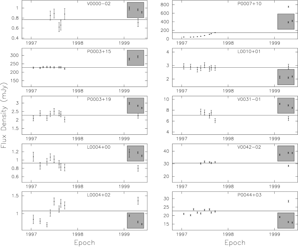
Figure 1: VLA X-band (8.48 GHz) radio light curves for quasars from the target sample. The inset boxes show the radio spectrum at L-, C-, and X-bands (1.49, 4.89, and 8.48 GHz respectively), going from left to right. The horizontal line running through the center of each plot represents the mean value of the X-band flux density for that source. In most cases the vertical axis is scaled to run from 0.5 to 1.5 times the mean flux density.

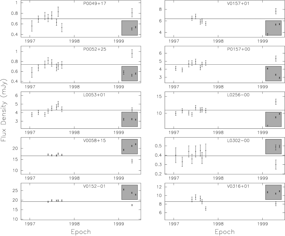
Figure 1 (cont):

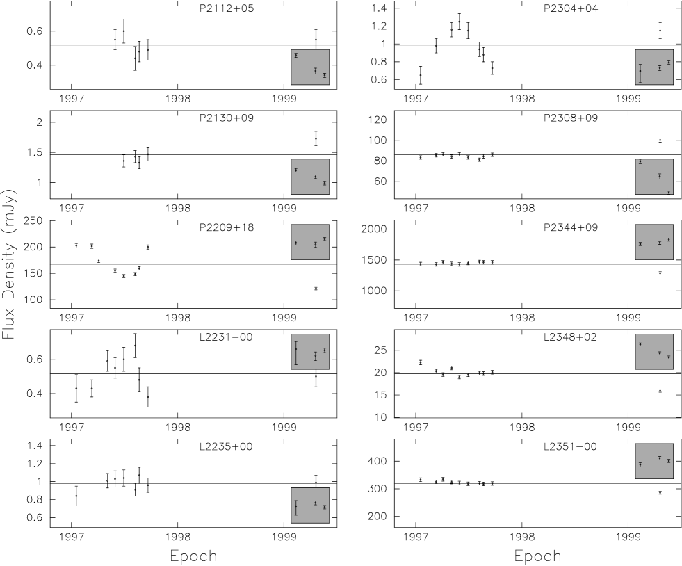
Figure 1(cont):

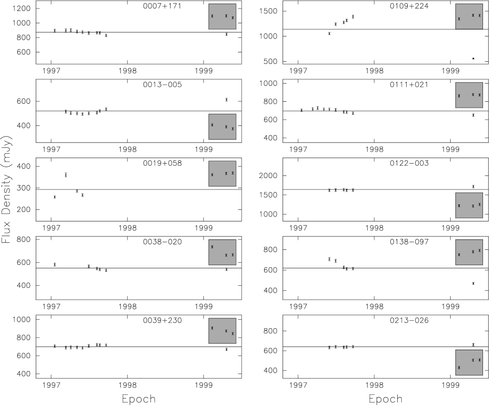
Figure 2: Same as Figure 1, but for the calibrator sources.

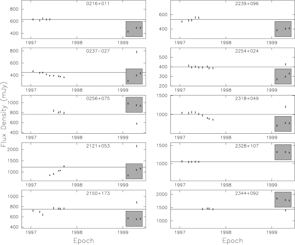
Figure 2(cont):

Figure 3: Debiassed variability index $V_{RMS}$, expressed in percent, versus radio-to-optical flux density ratio $R$. The plot is divided into regions of radio quiet, radio intermediate, and radio loud objects. The mean radio flux density over all epochs is used in the calculation of $R$. The closed symbols represent target quasars, while the open circles represent calibrators. The variability index of III Zw 2 – the highest point in the diagram – is shown here only as a lower limit (actual value 140.9) to keep the scale of the plot in reasonable bounds. We define the variability index to be negative in cases where the actual fluctuations are smaller than expected from the error bars, due either to chance or to overestimation of the errors (see text).

Figure 4: Debiassed variability index $V_{RMS}$ versus radio luminosity. Symbols are the same as in Figure 3: closed triangles for RQQs, closed squares for RIQs, closed circles for RLQs, and open circles for calibrators. Four calibrators are not plotted because they lack redshifts.

Figure 5: Debiassed variability index $V_{RMS}$ versus optical luminosity. Symbols same as in Figure 4.

Figure 6: Debiassed variability index $V_{RMS}$ versus redshift. Symbols same as in Figure 4.

Figure 7: Debiassed variability index $V_{RMS}$ versus radio spectral index between C- and X-band. Symbols same as in Figure 4.

Figure 8: Comparison of histograms of debiased RMS for the four source classes. Here we have set negative values to zero, since such values mean that the sources were not variable. This is indicated by the asterix in $V^{*}_{RMS}$. Value for III Zw 2 is off the scale of the abscissa (indicated by arrow).

Figure 9: Comparison of radio spectral index histograms for the four source classes.

References

- (1) Akritas, M.G., & Bershady, M.A. 1996, ApJ, 470, 706
- (2) Aller, M.F., Aller, H.D., Hughes, P.A., & Latimer, G.E. 1999, ApJ, 512, 601
- (3) Barvainis, R., Lonsdale, C., & Antonucci, R. 1996, AJ, 111, 1431
- (4) Barvainis, R., & Lonsdale, C. 1997, AJ, 113, 144
- (5) Becker, R.H., et al. 2001, ApJS, 135, 227
- (6) Bischof & Becker, R.H. 1997, AJ, 113, 2000
- (7) Blandford, R.D., astro-ph/0001499
- (8) Blundell, K.M., Beasley, A., Lacy, M., & Garrington, S.T. 1996, ApJ, 468, L91 1998, MNRAS, 299, 165
- (9) Blundell, K.M., & Rawlings, S. 2001, ApJ, 562, L5
- (10) Blundell, K.M., & Beasley, T. 1998, MNRAS, 299, 165
- (11) Blundell, K.M., Beasley, T., & Bicknell, G.V. 1993, ApJ, 591, L103
- (12) Cirasuolo, M., Celotti, A., Magliocchetti, M., & Danese, L. 2003, astro-ph/0306415
- (13) Dunlop, J.S., McLure, R.J., Kukula, M.J., Baum, S.A., O’Dea, C.P., & Hughes, D.H. 2003, MNRAS, 340, 1095
- (14) Falcke, H., Sherwood, W., & Patnaik, A.R. 1996, ApJ, 471, 106
- (15) Falcke, H., Patnaik, A.R., Sherwood, W. 1996, ApJ, 473, 13
- (16) Falcke, H., et al. 1999, ApJ, 514, L17
- (17) Falco, E.E., Lehar, J., Perley, R. A., Wambsganss, J., & Gorenstein, M. V. 1996, AJ, 112, 897
- (18) Fanaroff, B.L., & Riley, J.M. 1974, MRAS, 298, 395
- (19) Floyd, D.J.E., et al. astro-ph/0308436
- (20) Goldschmidt, P., Miller, L., La Franca, F., & Cristiani, S. 1992, MNRAS, 256, 65p
- (21) Goldschmidt, P., Kukula, M. J., Miller, L., & Dunlop, J. S. 1999, ApJ, 511, 612
- (22) Ho, L.C.; van Dyk, S.D., Pooley, G.G., Sramek, R.A., & Weiler, K.W. 1999, AJ, 118, 843
- (23) Hooper, E.J., Impey, C.D., Foltz, C.B., & Hewett, P.C. 1995, ApJ, 445, 62
- (24) Hooper, E.J., Impey, C.D., Foltz, C.B., & Hewett, P.C. 1996, ApJ, 473, 746
- (25) Hutchings, J. B.; Gower, A. C.; Ryneveld, S.; Dewey, A. 1996 AJ, 111, 2167
- (26) Ivezic, Z., et al. 2002, AJ, 124, 2364
- (27) Kellermann, K.I., Sramek, R., Schmidt, M., Shaffer, D.B., & Green, R. 1989, AJ, 98, 1195
- (28) Kellermann, K.I., Sramek, R.A., Schmidt, M., Green, R.F., & Shaffer, D. B. 1994, AJ, 108, 1163
- (29) McLure, R.J, & Dunlop, J.S. 2001, MNRAS, 321, 515
- (30) Miller, L., Peacock, J.-A., & Mead, A. 1990, MNRAS, 244, 207
- (31) Miller, P., Rawlings, S., & Saunders, R. 1993, MNRAS, 263, 425
- (32) Readhead, A.C.S. 1994, ApJ, 426, 51
- (33) Shields, G.A., et al. 2003, ApJ, 124, 133
- (34) Sopp, H.M., & Alexander, M.N. 1991, MNRAS, 251, 14p
- (35) Stocke, J.T., Morris, S.L., Weymann, R.J., & Foltz, C.B. 1992, ApJ, 396, 487
- (36) Strittmatter, P.A., Hill, P., Pauliny-Toth, I.I.K., Steppe, H., & Witzel, A. 1980, A&A, 88, L12
- (37) Terlevich, R., Tenorio-Tagle, G., Franco, J., & Melnick, J. 1992, MNRAS, 255, 713
- (38) Ulvestad, J., Antonucci, R. & Barvainis, R. 2004, in prep.
- (39) Visnovsky 1992, ApJ, 391, 560
- (40) Wagner, S.J., & Witzel, A. 1995, ARA&A, 33, 163
- (41) White, R.L., Becker, R.H., Gregg, M.D., et al. 2000, ApJS, 126, 133
- (42) Wilson, A.S., & Colbert, E.J.M. 1995, ApJ, 438, 62
- (43) Wold, M., Lacy, M., Lilje, P.B., & Serjeant, S. 2001, MNRAS, 323, 231