Is there a Dichotomy in the Radio Loudness Distribution of Quasars ?

Abstract

We present a new approach to tackle the issue of radio loudness in quasars. We constrain a (simple) prescription for the intrinsic distribution of radio-to-optical ratios by comparing properties of Monte Carlo simulated samples with those of observed optically selected quasars. We find strong evidence for a dependence of the radio luminosity on the optical one, even though with a large scatter. The dependence of the fraction of radio loud quasars on apparent and absolute optical magnitudes results in a selection effect related to the radio and optical limits of current surveys.
The intrinsic distribution of the radio-to-optical ratios shows a peak at $R^{*}_{1.4}\sim 0.3$, with only $\mathrel{\hbox to0.0pt{\lower 3.0pt\hbox{$\sim$}\hss}\raise 2.0pt\hbox{$<$}}5$  per cent of objects being included in a high $R^{*}_{1.4}$ tail which identifies the radio loud regime. No lack or deficit of sources – but only a steep transition region – is present between the radio loud and radio quiet populations at any $R^{*}_{1.4}$. We briefly discuss possible origins for this behaviour (e.g. absence of jets in radio quiet sources, large range of radiative radio efficiency, different life-times for the accretion and jet ejection phenomena, …).

1 INTRODUCTION

The origin of radio loudness of quasars is a long debated issue. Radio observations of optically selected quasar samples showed only 10-40 % of the objects to be powerful radio sources (Sramek & Weedman 1980; Condon et al. 1981; Marshall 1987; Miller, Peacock & Mead 1990; Kellermann et al. 1989). More interestingly, these early studies suggested that quasars could be divided into the two populations of “Radio-Loud” (RL) and “Radio-Quiet” (RQ) on the basis of their radio emission. Furthermore, Kellermann et al. (1989) found that the radio-to-optical ratios, $R^{*}_{1.4}$ , of these objects presented a bimodal distribution. Miller, Peacock & Mead (1990) also found a dichotomy in the quasar population, although this time radio luminosity was used as the parameter to define the level of radio loudness.

In the last decade, our ability of collecting large samples of quasars with faint radio fluxes has grown enormously, in particular thanks to the FIRST (Faint Images of the Radio Sky at Twenty centimeters) Survey at VLA (Becker, White & Helfand 1995). However, despite the recent efforts, radio loudness still remains an issue under debate. Works based on data from the FIRST survey (White et al. 2000; Hewett et al. 2001) suggest that the found RL/RQ dichotomy could be due to selection effects caused by the brighter radio and optical limits of the previous studies. On the contrary, Ivezic et al. (2002) seem to find evidence for bimodality in a sample drawn from the Sloan Digital Sky Survey. More recently Cirasuolo et al. (2002) (hereafter paper I) – analyzing a new sample obtained by matching together the FIRST and 2dF QSO Redshift Survey – ruled out the classical RL/RQ dichotomy in which the distributions of radio-to-optical ratios and/or radio luminosities show a deficit of sources, suggesting instead a smoother transition between the RL and the RQ regimes.

Also from the interpretational point of view, the physical mechanism(s) responsible for radio emission in Active Galactic Nuclei (AGN) is still debated. At least for RL quasars it is generally accepted to be related to the process of accretion onto a central black hole (BH) – the engine responsible for the optical-UV emission – via the formation of relativistic jets which can be directly imaged in nearby objects. The connection between the optical (accretion) and radio (jet) emission is however unclear. Phenomenologically there is indication in RL objects of correlations between radio emission and luminosity in narrow emission lines, produced by gas presumably photoionized by the nuclear optical–UV continuum (e.g. Rawlings & Saunders 1991). Results from paper I show that, for a given optical luminosity, the scatter in radio power is more than three orders of magnitude. Note that if quasars are AGN accreting near the Eddington limit, this result tends to exclude the mass of the central BH as the chief quantity controlling the level of radio activity (see also Woo & Urry 2002), although we cannot conclude anything on the possible presence of a threshold effect, whereby RL AGN would be associated to the more massive BH ($M_{\rm BH}>1-5\times 10^{9}M_{\odot}$, Laor 2000, Dunlop et al. 2002, but see also Woo & Urry 2002 for a dissenting view). On the other hand, although controversial, there is some evidence for the fraction of RL quasars to increase with increasing optical luminosity (Padovani 1993; La Franca et al. 1994; Hooper et al. 1995; Goldschmidt et al. 1999; paper I; but see also Ivezic et al. 2002 for a different view).

Clearly, the uncertainties on the presence of a dichotomy, the character of radio loudness and the consequent poor knowledge of its origin (dependence on BH mass, optical luminosity etc.) are due to the analysis of different samples, often very inhomogeneous because of selection effects both in the optical and radio bands, i.e. the lack of a single sample covering all the ranges of optical and radio properties of quasars.

Therefore, in order to shed light on this issue, we adopted the alternative approach of starting from simple assumptions on the intrinsic properties of the quasar population as a whole – namely an optical quasar luminosity function and a prescription to associate a radio power to each object - and, through Monte Carlo simulations, generate unbiased quasar samples. By applying observational limits in redshift, apparent magnitude and radio flux we can then compare the results of the simulations with the properties of observed samples. The aim of this approach is of course twofold: constrain the initial hypothesis on the intrinsic nature of quasars, by requiring properties of the simulated samples – such as $R^{*}_{1.4}$ and radio power distributions, fraction of radio detections etc. – to be in agreement with the observed ones; test the effects of the observational biases on each sample by simply changing the observational limits.

The layout of the paper is the following. In Section 2 we briefly present the samples used to constrain the models, while in Section 3 we describe the procedures adopted to generate simulated samples. In Section 4 results of the simulations and comparisons of the properties of the observed and simulated samples are shown. We discuss the physical meaning of these results and summarize our conclusions in Section 5. Throughout this work we will adopt $H_{0}=$ 50 km s^-1 Mpc^-1, $q_{0}=0.5$ and $\Lambda=0$.

2 The Datasets

As there is not (yet) a single sample able to cover, with enough statistics and completeness, the total range of known radio activity (e.g. the distribution of radio-to-optical ratios and/or radio powers), we have to consider various samples to constrain - as completely as possible - the properties of our simulated samples. We choose three samples of optically selected quasars, namely the 2dF Quasar Redshift Survey (2dF), the Large Bright Quasar Survey (LBQS) and the Palomar Bright Quasar Survey (PBQS). These have in fact a high completeness level and are quite homogeneous since all of them are optically selected in the blue band and have a similar radio cut. The 2dF and LBQS have been cross-correlated with the FIRST survey with a limiting flux at 1.4 GHz of 1 mJy, while the PBQS has been observed at 5 GHz down to a limiting flux of 0.25 mJy, which is comparable to the 1 mJy flux limit at 1.4 GHz, for a typical radio spectral index $\alpha_{\rm R}=0.8$ . Equally crucial for our work is the fact that these samples produce a very large coverage of the optical luminosity-redshift plane and provide information on different regimes of radio activity (see Fig.1).

Here we briefly describe the main characteristics of the three samples. In order to have complete homogeneity and favour the comparison with simulations, for each sample we have only considered the ranges in redshift, apparent magnitude and radio flux with the highest completeness. We have also selected sources with $M_{\rm B}\leq-23$ to avoid contaminations from the host galaxy light (Croom et al. 2001; paper I) and we have applied a mean correction of 0.07 mag to convert $b_{\rm J}$ to B magnitudes (see paper I), on the basis of the composite quasar spectrum compiled by Brotherton et al. (2001). The same composite spectrum has also been used to compute the k-correction in the B band.

2.1 2dF Quasar Redshift Survey

We have used the first public release of the 2dF QSO Redshift Survey, the so called 2QZ 10k catalogue. Here we briefly recall its main properties, while a complete description can be found in Croom et al. (2001). QSO candidates with $18.25\leq b_{\rm J}\leq 20.85$ were selected from the APM catalogue (Irwin, McMahon & Maddox 1994) in two $75^{\circ}\times 5^{\circ}$ declination strips centered on $\delta=-30^{\circ}$ and $\delta=0^{\circ}$, with colour selection criteria $(u-b_{\rm j})\leq 0.36$; $(u-b_{\rm j})<0.12-0.8\;(b_{\rm j}-r)$; $(b_{\rm j}-r)<0.05$. Such a selection guarantees a large photometric completeness ($>90$ per cent) for quasars within the redshift range $0.3\leq z\leq 2.2$. The final catalogue contains $\sim 21,000$ objects with reliable spectral and redshift determinations, out of which $\sim 11,000$ are quasars ($\sim 53$ per cent of the sample).

As extensively described in paper I, this sample has been cross-correlated with the FIRST survey (Becker et al. 1995). The overlapping region between the FIRST and 2dF Quasar Redshift Surveys is confined to the equatorial plane: $9^{h}\;50^{m}\leq{\rm RA(2000)}\leq 14^{h}\;50^{m}$ and $-2.8^{\circ}\leq{\rm dec(2000)}\leq 2.2^{\circ}$. For the matching procedure a searching radius of 5 arcsec and an algorithm to collapse multiple-component radio sources (jets and/or hot-spots) into single objects were used. (Magliocchetti et al. 1998). The resulting sample is constituted by 113 objects, with optical magnitudes $18.25\leq b_{\rm j}\leq 20.85$ and radio fluxes at 1.4 GHz $S_{1.4{\rm GHz}}\geq 1$ mJy, over an effective area of 122.4 square degrees. In the following we consider the sub-sample (hereafter called the FIRST-2dF sample) containing 89 objects with absolute magnitudes brighter than $M_{\rm B}\leq-23$ spanning in the redshift range $0.35\leq z\leq 2.1$.

2.2 Large Bright Quasar Survey

The Large Bright Quasar Survey (LBQS) comes as the natural extension to brighter magnitudes of the 2dF sample since it has been derived with the same selection criteria. A detailed description of this survey can be found in Hewett et al. (1995). It consists of quasars optically selected from the APM catalogue (Irwin et al. 1994) at bright ($b_{\rm j}<19$) apparent magnitudes. Redshift measurements were subsequently derived for 1055 of them over an effective area of 483.8 square degrees. Due to the selection criteria of the survey, quasars were detected over a wide redshift range ($0.2\leq z\leq 3.4$), with a degree of completeness estimated to be at the $\sim 90$ per cent level.
More recently, this sample was cross-correlated with the FIRST survey (Hewett et al. 2001) by using a searching radius of 2.1 arcsec over an area of the sky of 270 square degrees. This procedure yielded a total of 77 quasars with radio fluxes $S_{1.4{\rm GHz}}\geq 1$ mJy, magnitudes in the range $16\mathrel{\hbox to0.0pt{\lower 3.0pt\hbox{$\sim$}\hss}\raise 2.0pt\hbox{$<$}}b_{\rm j}\mathrel{\hbox to0.0pt{\lower 3.0pt\hbox{$\sim$}\hss}\raise 2.0pt\hbox{$<$}}19$ and with a fractional incompleteness of $\sim 10$ per cent. For homogeneity with the FIRST-2dF, out of this sample we have only considered 58 sources with apparent magnitudes $16\leq b_{\rm j}\leq 18.8$ and redshifts $0.2\leq z\leq 2.2$, all of them with $M_{\rm B}\leq-23$ (hereafter called the FIRST-LBQS sample).

2.3 Palomar Bright Quasar Survey

We have also considered the Palomar Bright Quasar Survey (Schmidt & Green 1983), which represents one of the historical and most studied sample of quasars, in order to cover the very bright end of the absolute magnitude distribution. It contains 114 objects brighter than an effective limiting magnitude $B=16.16$, selected over an area of 10,714 square degrees using the UV excess technique. Such quasars have been observed using the VLA at 5 GHz with 18 arcsec resolution, down to a flux limit of 0.25 mJy ($4\sigma$) (Kellermann et al. 1989). In order to reduce, as much as possible, the contamination due to the host galaxy, we have chosen not to consider the very local sources with redshift $z<0.1$. Our choice is also justified by the fact that all these objects are classified as “galaxy” in the NED archive (NASA/Ipac Extragalactic Database), indicating that the host galaxy is clearly visible. Again, for homogeneity with the former datatsets, from this sample we have only selected objects with $13\leq B\leq 16.16$, in the redshift range $0.1\leq z\leq 1.5$, with $M_{\rm B}\leq-23$ and radio flux $S_{\rm 5GHz}\geq 0.25$ mJy, ending up with a sub-sample of 48 radio sources (hereafter called the PG sample).

Figure 1: Distributions of the radio-to-optical ratios for the three samples: FIRST-2dF (solid line), FIRST-LBQS (dotted line) and PG (dashed line)

3 Monte Carlo Simulations

As already mentioned, as selection effects both in the optical and in the radio bands bias each of the samples introduced in Section 2 with respect to the quasar radio properties, our approach is to start from simple assumptions on the intrinsic features of the quasar population and test them by comparing results from simulated samples – generated through Monte Carlo realizations – with those of the observed samples. We decided to assume as the two fundamental ingredients to describe the quasar population a well defined Optical Luminosity Function (OLF) - from which to obtain redshift and optical magnitude for the sources - and a distribution of radio-to-optical ratios which provides each source with a radio luminosity.
Here we briefly specify these assumptions and describe the procedure applied in our Monte Carlo simulations.

3.1 Optical Luminosity Function

The best determined OLF for the whole quasar population currently available is the one obtained from the 2dF Quasar Redshift Survey (Boyle et al. 2000; Croom et al. 2001), based on $\sim 11,000$ sources. This can be described as a broken power-law (Croom et al. 2001)

$$\phi(M_{\rm B},z)=\frac{\phi^{*}}{10^{0.4[C(z)(\alpha+1)]}+10^{0.4[C(z)(\beta+1)]}},$$ (1)

with $\alpha=3.28$, $\beta=1.08$, $C(z)=M_{\rm B}-M_{\rm B}^{*}(z)$, where sources undergo a pure luminosity evolution parametrized by the expression

$$M_{\rm B}^{*}(z)=M_{\rm B}^{*}(0)-2.5(k_{1}z+k_{2}z^{2}),$$ (2)

with $k_{1}=1.41$, $k_{2}=-0.29$ and $M_{\rm B}^{*}(0)=-21.45$. One of the main advantages of using this luminosity function is that it has been obtained in the B band and over the wide redshift range $0.35\leq z\leq 2.2$, therefore reducing the need for extrapolations, which would add further uncertainties. Some extrapolation is instead needed for the bright end of the luminosity function ($M_{B}\mathrel{\hbox to0.0pt{\lower 3.0pt\hbox{$\sim$}\hss}\raise 2.0pt\hbox{$<$}}-27$), which is not well sampled by the available data. Adopting the above OLF we have then randomly generated sources, over redshift and apparent magnitude ranges necessary to compare them with each of the three samples.

Note that, we have used the Optical LF as a description of the key quasar properties and number density mainly because we are going to compare our results with samples of optically selected quasars. In a more general picture one should also include the contribution to the quasar population given by the obscured (type II) QSO. To this aim it would be plausibly more appropriate to use a hard X-ray LF, which however so far has only been computed for type I objects (La Franca et al. 2002) and which thus results to be similar in shape and evolution to the one determined in the soft X-ray band (Miyaji et al 2000). We stress that, since the radio emission is not affected by obscuration, the contribution of type II quasars would affect our results (e.g. the distribution of radio-to-optical ratios) only if there was a dependence of the obscuration level on the quasar optical luminosity. However, as recent results (La Franca et al. 2002; Tozzi et al. 2001; Giacconi et al. 2002; Rosati et al. 2002) seem to suggest, the fraction of these obscured quasars is expected to be small when compared to the unobscured ones. The above conclusion implies that the presence of type II quasars should not significantly affect our findings and therefore we have decided to neglect their (uncertain) contribution.

3.2 Radio vs Optical Luminosity

The other ingredient needed for our analysis is a relation between optical and radio luminosities. As already concluded in paper I, although present, this shows a wide spread: Figure 2 illustrates – for the objects in the three samples considered in this work – how sources with a particular optical luminosity can be endowed with radio powers spanning up to three orders of magnitude.

We have thus taken into account two (simple) different scenarios. The first one assumes a relation between radio and optical luminosity, although with a large scatter (Model A); in this case we use a distribution in $\log_{10}(R^{*}_{1.4})$ and compute the radio power as $\log_{10}(R^{*}_{1.4})+\log_{10}(L_{\rm opt})$. The second case describes the possibility for the radio luminosity to be completely unrelated to the optical one, and assume a distribution in $\log_{10}(L_{\rm radio})$ for any given optical luminosity (Model B). For Models A and B respectively, we then consider different shapes for the distribution of radio-to-optical ratios and radio luminosities: a) the simplest case of a flat uniform distribution over the whole range of radio-to-optical ratios or radio powers; b) a single Gaussian distribution, in which the RL regime could simply represent its tail; c) two Gaussians, the first peaked in the RL regime and the second in the RQ one, in order to allow for a more flexible shape of the distributions and test the hypothesis of bimodality.

As a final step, radio flux densities have been computed from radio powers by assuming 80 per cent of these sources to be steep spectrum ($\alpha_{\rm R}=0.8$), while the others to be flat spectrum ($\alpha_{\rm R}=0$) objects. These fractions have been chosen according to the results found in paper I: although for the FIRST-2dF sample we only managed to compute the radio spectral index for the ten most luminous objects, roughly finding the same fraction of steep and flat spectra, the remaining sources do not have any counterpart at radio frequencies $>1.4$ GHz, suggesting that most of the quasars have a steep spectrum. These assumed fractions are also in agreement with that of steep spectrum sources observed in the PG sample.

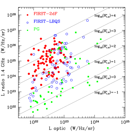
Figure 2: Optical versus radio luminosity for sources in the considered samples. The dotted lines are loci of constant radio-to-optical ratio.

It must be noticed that in these associations of a radio luminosity to each optical quasar there is a strong implicit assumption on the evolution, namely that radio and optical luminosities evolve in the same way. Even though we have no direct evidence, some hints supporting this hypothesis can be bound from the data. On one side in paper I it has been shown that the $R^{*}_{1.4}$ distribution, both for sources in the FIRST-2dF and in the FIRST-LBQS, is completely independent of redshift. This is not expected if radio and optical luminosities had significantly different evolutions. On the other side, an independent indication of such hypothesis is obtained from the $<V/V_{\rm max}>$ test, which we applied separately to radio detected objects (from the FIRST-2dF) and to quasars representative of the population as a whole (from the total 2dF). For objects in the radio sample we computed $V_{\rm max}$ by using the maximum redshift at which a source could have been included both in the radio and in the optical datasets, given the radio flux and optical magnitude limits. We considered three redshift bins and the results are reported in Table 1. The values of $<V/V_{\rm max}>$ for the two populations are perfectly compatible in all redshift bins, even though the errors for the radio sample are larger due to the smaller number of objects. This again suggests the evolutionary behaviour of the radio detected and total populations to be similar, justifying our assumption.

z	Total	Radio
0.35 - 1	$0.61\pm 0.01$	$0.58\pm 0.07$
1 - 1.5	$0.55\pm 0.01$	$0.53\pm 0.05$
1.5 - 2.1	$0.51\pm 0.008$	$0.50\pm 0.05$

Table 1: Mean $V/V_{\rm max}$ values for the radio detected and the total quasar population from the 2dF sample as measured in three different redshift bins.

3.3 Constraints from the data

Adopting each of the six models described in the previous section and applying the observational limits (reported for clarity in Table 2), we have simulated samples of radio emitting quasars. Comparisons with the FIRST-2dF, FIRST-LBQS and PG samples provide several constraints. In particular the simulated populations must reproduce the observed:

• distributions of radio-to-optical ratios and radio powers. The three samples identify different levels of radio activity: while the FIRST-2dF – which is the optically faintest – well traces the RL regime for $R^{*}_{1.4}\mathrel{\hbox to0.0pt{\lower 3.0pt\hbox{$\sim$}\hss}\raise 2.0pt\hbox{$>$}}50$, the FIRST-LBQS is sensible to the RL-RQ transition and the PG is particularly suited to constrain the RQ regime (see Figure 1).

• fraction of radio detections. As shown in Figure 3, this fraction depends on the optical limiting magnitude of the survey: from $\sim 3$ per cent for the optically faint sources (FIRST-2dF), to $\sim 20$ per cent for objects with $B\sim 17$ (FIRST-LBQS) and up to 70 per cent or more at the brightest magnitudes (PG).
  Note that a similar dependence is also followed by the intrinsic luminosity, as the fraction of radio detections grows from $\mathrel{\hbox to0.0pt{\lower 3.0pt\hbox{$\sim$}\hss}\raise 2.0pt\hbox{$<$}}3$ per cent at $M_{\rm B}\sim-24$ up to 20-30 per cent for the brightest $M_{\rm B}\sim-28$ objects (paper I; Padovani 1993; La Franca et al. 1994; Hooper et al. 1995; Goldschmidt et al. 1999).

• number counts, both in the radio and in the optical band.

• redshift and absolute magnitude distributions.

Survey	$N_{\rm QSO}$	$z_{\rm lim}$	$B_{\rm lim}$	$S_{\rm lim}$ (mJy)	Area (deg2)
FIRST-2dF	89	$0.35\leq z\leq 2.1$	$18.25\leq b_{\rm j}\leq 20.85$	$S_{\rm 1.4\>GHz}\geq 1$	122.4
FIRST-LBQS	58	$0.20\leq z\leq 2.2$	$16.00\leq b_{\rm j}\leq 18.80$	$S_{\rm 1.4\>GHz}\geq 1$	270.0
PG	48	$0.10\leq z\leq 1.5$	$13.00\leq B\leq 16.16$	$S_{\rm 5\>GHz}\geq 0.25$	10714.0

Table 2: Selection limits and covered areas for the surveys used in our analysis. $N_{\rm QSO}$ is the number of quasars with $M_{\rm B}\leq-23$

Figure 3: Fraction of quasars with a radio counterpart in the three samples as a function of the apparent optical magnitude.

4 Results

Monte Carlo simulations have been run exploring the widest range of values for the free parameters – which describe the distributions of radio-to-optical ratios (Model A) or radio powers (Model B) – in order to find all the sets of values able to reproduce the data. We have used simulated samples with a hundred times more objects than the original datasets and the realizations have been repeated with different initial seeds, in order to minimize the errors on the simulated quantities. We tested the validity of each model by comparing the properties of simulated and observed samples through statistical tests: a Kolmogorov-Smirnov (KS) test for the $R^{*}_{1.4}$ and radio power distributions, and a $\chi^{2}$ test for the fraction of radio detections as a function of apparent and absolute magnitude, and also for the optical and radio number counts.

4.1 Results for flat and single Gaussian distributions

We find that the simplest model, a flat distribution, is totally inconsistent with the data and rejected by the statistical tests, both for Model A and B. In particular it is unable to reproduce the observed number counts for the three samples simultaneously: the data, in fact, require the number of RL quasars to be less than the RQ ones, while this distribution spreads objects uniformly.
We then tested the single Gaussian distribution, which also fails, for both Model A and B, mainly because it is unable to simultaneously reproduce the observed distribution of $R^{*}_{1.4}$ in the RL regime and the total number of objects in the three samples.

4.2 Results for the two-Gaussian distribution

Given the above difficulties, we considered the more flexible model of two Gaussians, respectively centered in the RL and RQ regions. As said, each one of the considered samples traces different radio regimes: in particular the FIRST-2dF sample well constrains the shape of the distribution at high $R^{*}_{1.4}$, and also – through the number counts – well determines the fraction of objects with high levels of radio emission. As a consequence, the parameters of the first Gaussian (center $x_{1}$ and dispersion $\sigma_{1}$) and the relative fraction of objects in the two Gaussians are mainly determined by this sample. The other two samples constrain parameters of the second Gaussian in the RQ regime: the PG sample mainly determines its peak position; the FIRST-LBQS sample – which traces the transition region between RL and RQ – constrains quite well the shape of the wing of the second Gaussian and its overlap with the first one.

$x_{1}$	$\sigma_{1}$	$x_{2}$	$\sigma_{2}$	Fraction
$2.7\pm 0.2$	$0.7\pm 0.2$	$-0.5\pm 0.3$	$0.75\pm 0.3$	$97\pm 2$ per cent

Table 3: Best fit parameters for Model A, expressed in $\log_{10}\>R^{*}_{1.4}$. $x_{1}$ and $\sigma_{1}$ are the center and dispersion of the Gaussian in the RL regime, while $x_{2}$ and $\sigma_{2}$ are those for the Gaussian in the RQ one. “Fraction” indicates the percentage of objects having radio-to-optical ratios described by the second Gaussian. Errors have been obtained as explained in Section 4.2

Figure 4: Distribution of radio-to-optical ratios (top panel) and of radio powers (bottom panel) obtained from the best-fit set of parameters of Model A (see Table 3). The distributions are plotted in binned form and the shaded regions indicate the range of $R^{*}_{1.4}$ and $P_{1.4}$ for which no data are available.

• Model B. In this case, i.e. radio luminosity completely unrelated to the optical one, no set of parameters has been found able to satisfy the statistical tests for all the observed quantities. In particular, this model is not able to predict the growing fraction of radio detections as a function of both apparent and absolute magnitudes, and to reproduce in a satisfactory way the shapes of the radio-to-optical ratio distributions simultaneously in the case of FIRST-2dF and FIRST-LBQS.
  

• Model A. A promising solution has been found in this case, namely by assuming radio and optical luminosities to be related even though with a large scatter. The radio-to-optical ratio and radio power distributions corresponding to this solution are displayed in Figure 4 and the model parameters are given in Table 3. A comparison between the properties of observed and simulated samples is shown in Figures 5 and 6. We find a good agreement with the $R^{*}_{1.4}$ and radio power distributions of the FIRST-2dF and FIRST-LBQS samples (high KS probabilities, from 0.2 up to 0.9, for the distributions in Figure 5). The simulated datatset is also able to reproduce the observed fraction of radio detections, both as a function of apparent and absolute magnitudes (with a significance level for the $\chi^{2}$ test $>0.05$ see Figure 6) and the number counts, except for a tendency – compatible within the errors – to over-estimate the FIRST-2dF and correspondingly under-estimate the FIRST-LBQS counts.
  However, substantial disagreement is found for the $R^{*}_{1.4}$ and radio power distributions when compared to the observed quantities in the PG sample (KS probabilities $<10^{-2}$). The discrepancy is mainly due to the presence in this sample of $\sim 10$ objects with high values of $R^{*}_{1.4}$ ($\mathrel{\hbox to0.0pt{\lower 3.0pt\hbox{$\sim$}\hss}\raise 2.0pt\hbox{$>$}}100$), which also determine the different shape of the radio number counts (see Figure 6). We stress that we found no solution compatible with both the PG and the other two samples: the excess of RL sources in the PG dataset is in fact inconsistent with the both FIRST-2dF and FIRST-LBQS samples. We therefore investigated in more details the properties of these $\sim 10$ PG sources, by looking at their radio and optical-to-X-ray spectral indices and the compactness of the radio emission. We found the properties of these quasars to be completely indistinguishable from those of other objects in the PG sample, except for a slightly different redshift distribution (these RL quasars are mainly concentrated in the range $0.3\leq z\leq 0.5$) and (by definition) their high $R^{*}_{1.4}$. We notice however that it has been shown that the PG sample is incomplete (Goldschmidt et al. 1992) and it has also been suggested this incompleteness not to be random with respect to the radio properties (Miller, Rawlings & Saunders 1993; Goldschmidt et al. 1999). Because of this we are more confident that the FIRST-2dF and FIRST-LBQS are better suited to represent the shape of the $R^{*}_{1.4}$ distribution, at least in the RL regime. Due to these problems with the PG sample, we have therefore not considered the constraints on the $R^{*}_{1.4}$ and radio power distributions for this sample, converging to the same best fit model as discussed before.

  As a further test we have looked at the redshift and absolute magnitude distributions. The comparison between data and model predictions is shown in Figure 7, which reveals an excellent agreement in the case of the FIRST-2dF sample. A worse accordance has been found for the other datasets, even though the simulated vs. observed distributions are still compatible within the errors. The simulated samples (in these two cases) reveal a tendency to overproduce objects at bright ($M_{B}\mathrel{\hbox to0.0pt{\lower 3.0pt\hbox{$\sim$}\hss}\raise 2.0pt\hbox{$<$}}-27$) absolute magnitudes, probably due to the extrapolation of the bright end of the luminosity function (see Section 3.1). However, we want to stress that this effect cannot explain the disagreement in the $R^{*}_{1.4}$ and radio power distributions found for the PG sample. In fact, those RL sources found to be in excess with respect to the expectations – and clearly visible in the redshift bin at $z\sim 0.4$ – have absolute magnitudes $-25\mathrel{\hbox to0.0pt{\lower 3.0pt\hbox{$\sim$}\hss}\raise 2.0pt\hbox{$<$}}M_{B}\mathrel{\hbox to0.0pt{\lower 3.0pt\hbox{$\sim$}\hss}\raise 2.0pt\hbox{$<$}}-26$, a range in which the OLF is well defined.

Figure 5: Comparison between the observed (dotted lines) and the predicted (solid lines) distributions of radio-to-optical ratios (on the left) and radio powers (on the right) for the three samples. Error-bars on the observed distributions are derived by assuming a Poissonian distribution.

Figure 6: Left panels: Comparison between the observed (open circles) and the predicted (solid dots) fraction of radio detections for the three samples, as a function of the apparent and absolute magnitudes. Right panels: Comparison of the optical and radio integral number counts. Simbols are as in the former case.

Figure 7: Comparison between the observed (dotted lines) and expected (solid lines) distributions of redshift (on the left) and absolute magnitude (on the right).

Note that the above results have been obtained by relaxing the constraints for the PG sample only on the $R^{*}_{1.4}$ and radio power distributions, while still considering in the analysis the observed total number of objects and the fraction of radio detections: in fact, by completely eliminating this sample we would loose important and robust constraints on the RQ regime.

Finally we evaluate the ranges of acceptable parameters by varying their best fit values until one of the constraints (e.g. $R^{*}_{1.4}$ and radio power distributions, fraction of radio detections, etc.) was no longer satisfied with respect to the KS and/or $\chi^{2}$ tests. We adopted, as acceptable limits, a probability of 0.1 for the KS test and a confidence level of 0.05 for the $\chi^{2}$ test. In this way we obtained a reference error estimate on the parameters which is given in Table 3.

5 Discussion

The first point worth stressing is the “uniqueness” of the solution found. The combination of all the observational constraints is very cogent and thus, despite large errors on each constraint, we find that only one solution in the whole is able to simultaneously reproduce measurements from the three surveys. Furthermore, the uncertainties associated to the various parameters are in this case relatively small (see Table 3).
It is also intriguing to notice that a simple prescription for the distribution of the radio-to-optical ratios is able to well reproduce all of the available observational constraints given by three different samples. It is important to remark here that in order to reproduce the data we need a dependence of the radio luminosity on the optical one, even though with a large scatter. This is proved by the fact that Model B – where the two luminosities are completely unrelated – is rejected by the statistical tests. In particular, the successful model accounts for the dependence of the observed fractions of radio detected quasars on apparent and absolute optical magnitudes, as due to selection effects: going to optically fainter magnitudes (at a fixed radio flux limit) corresponds to selecting increasingly more RL objects. According to the model the intrinsic fraction of RL is small ($\mathrel{\hbox to0.0pt{\lower 3.0pt\hbox{$\sim$}\hss}\raise 2.0pt\hbox{$<$}}5$ per cent) when compared to the total population, and this e.g. explains the small fraction of radio detected quasars observed in the 2dF sample. Since the shape of the $R^{*}_{1.4}$ distribution (see Figure 4) is steep for $1\mathrel{\hbox to0.0pt{\lower 3.0pt\hbox{$\sim$}\hss}\raise 2.0pt\hbox{$<$}}R^{*}_{1.4}\mathrel{\hbox to0.0pt{\lower 3.0pt\hbox{$\sim$}\hss}\raise 2.0pt\hbox{$<$}}10$, surveys with brighter optical limiting magnitudes which select smaller values of $R^{*}_{1.4}$ (at a given radio flux) will then result in more and more radio detections. Similarly, the radio-optical dependence accounts for the flattening of the faint end of the optical luminosity function of RL quasars with respect to that of the whole population (La Franca 1994; Padovani 1993).

Given the uniqueness of the solution, the main result of this work is indeed the fact that we can put rather tight constraints on the intrinsic radio properties of quasars. The distributions shown in Figure 4 could then describe the unbiased view of the properties of the whole quasar population and this might possibly help us to understand the physical mechanism(s) responsible for the radio emission. First of all, in the $R^{*}_{1.4}$ distribution we note no lack or deficit of sources between the RL and RQ regimes: the distribution has a peak at $R^{*}_{1.4}\sim 0.3$ and decreases monotonically with a small fraction ($\mathrel{\hbox to0.0pt{\lower 3.0pt\hbox{$\sim$}\hss}\raise 2.0pt\hbox{$<$}}5$ per cent) of objects which are into the RL regime and represent a long tail of the total distribution. This result contrasts (see also paper I) the view of a RL/RQ dichotomy where a gap separates the two populations. Nevertheless we can still talk about a “dichotomy” in the sense that the data are compatible with an asymmetric distribution, with a steep transition region and with only a small fraction of sources having high values of $R^{*}_{1.4}$.

Then the basic questions are still open: do all sources belong to the same population? Or better: is there a single mechanism producing the radio emission in quasars or two different processes dominate in the bulk of the population and in the high $R^{*}_{1.4}$ tail? While it is believed that the radio emission in powerful radio quasars is produced in well collimated jets (related to accretion processes), it is not clear what is its origin in radio weaker and RQ sources. Let us then consider some of the possible interpretations.

First of all it is known that, because of relativistic beaming, the orientation of the source plays a leading role at least in the RL regime – although this could not account for the lack of large scale radio structures in RQ sources. In fact, relativistic boosting could push up by typically a factor of $10^{3}-10^{4}$ the observed radio emission (and correspondingly $R^{*}_{1.4}$ if the optical emission is dominated by thermal radiation). In this case we would expect at least the extreme RL sources to be flat spectrum, which is not supported by observations. A large fraction of the RL sources in the PG sample have a steep spectrum, and the same behaviour has been suggested for RL objects from the FIRST-2dF sample (paper I). Also well studied datasets of radio selected quasars, from the 2-Jy (Wall & Peacock 1985) and the 1-Jy samples (Stickel et al. 1994), show the distribution of radio-to-optical ratios to be the same for flat and steep spectrum radio quasars. However, this result could be affected by variability because of the non simultaneous radio flux measurements at different frequencies.

It has been proposed that the radio emission in RQ quasars is supplied by “starburst” phenomena, i.e. thermal emission from supernova remnants in a very dense environment (Terlevich et al. 1992). Alternatively, the radio flux could be associated to non-thermal emission from jets/outflows. In both cases we could reduce the presence of a dichotomy to the capability of the central engine to create a powerful/collimated jet. This in turn translates into the quest for identifying the parameter(s)/physical condition(s) responsible for its presence in only a few per cent of the sources.

As already mentioned, recent studies suggest the mass of the central BH not to be tightly related to the radio emission (paper I; Woo & Urry 2002), except for a possible threshold effect (Dunlop et al. 2002) which however has been recently questioned (Woo & Urry 2002). Also, radio loudness does not seem related to the properties of the host galaxy and of the environment (Dunlop et al. 2002), even though the latter claim is still debated. A further key physical parameter for the nuclear activity is the mass accretion rate: however it appears reasonable to assume that this is close to the Eddington limit for all powerful optical quasars. Still open possibilities instead include the hypothesis that the creation of a jet is related to a certain threshold in the BH spin or to the intensity and configuration of the magnetic field in the nuclear regions.

A clue on the origin of radio emission comes from the radio imaging at high resolution (pc scales) of RQ quasars, which revealed the presence of non–thermal emission from jet-like structures, even for objects with low ($R^{*}_{1.4}\sim 1$) radio loudness (Kukula et al. 1998; Blundell & Beasley 1998). In many objects have been resolved double or triple radio structures on scales of a few kiloparsecs. Moreover, the inferred high brightess temperatures ($T_{B}>10^{6}K$) suggest that the radio emission cannot be produced by a starburst. Then jets could be a common feature in quasars and the radio power level could be due to distributions in some of the jet properties, which however have to present a ‘threshold’ effect to reproduce the fast RQ/RL transition and RL tail. These properties could of course include the jet power or the efficiency of conversion of the jet energy into radiation. It has been suggested (Rawlings & Saunders 1991) that in powerful radio sources the power released into the jet is comparable to the accretion one. This would imply a radiative efficiency (in the radio band) of only about 0.1 - 1 per cent for RL quasars – and even less in RQ ones (Elvis et al. 1994). As a final remark we notice that also time dependence/evolution could play an important role: different ignition and duration times for the mechanisms responsible for the optical and radio emission could explain the observed distribution of radio-to-optical ratios. We are currently quantitatively comparing our results against these possible scenarios and the findings will be the subject of a forthcoming paper.

References

- [Becker et al.1995] Becker R.H., White R.L., Helfand D.J., 1995, ApJ, 450, 559
- [Blandford2000] Blandford R.D., 2000, PTRSA, astro-ph/0001499
- [Blundell] Blundell K.M. & Beasley A.J., 1998, MNRAS, 299, 165
- [Boyle et al.2000] Boyle B.J., Shanks T., Croom S.M., Smith R.J., Miller L., Loaring N., Heymans C., 2000, MNRAS, 317, 1014
- [Brotherton et al.2001] Brotherton M.S., Tran H.D., Becker R.H., Gregg M.D., Laurent-Muehleisen S.A., White R.,L., 2001, ApJ, 546,775
- [Cirasuolo et al.2002] Cirasuolo M., Magliocchetti M., Celotti A., Danese L., 2002, accepted by MNRAS, astro-ph/0301526 (paper I)
- [Condon et al.1981] Condon J.J., O’Dell S.L., Puschell J.J., & Stein W.A. 1981, ApJ, 246, 624
- [Croom et al.2001] Croom S.M., Smith R.J., Boyle B.J., Shanks T., Loaring N.S., Miller L., Lewis I.J., 2001, MNRAS, 322, L29
- [Dunlop et al.2002] Dunlop J.S., McLure R.J., Kukula M.J., Baum S.A., O’Dea C.P., Hughes D.H., 2002, astro-ph/0108397
- [Goldschmidt et al. 1992] Goldschmidt P., Miller L., La Franca F., Cristiani S., 1992, MNRAS, 256, 65p
- [Goldschmidt et al. 1999] Goldschmidt P., Kukula M.J., Miller L., Dunlop J.S., 1999, ApJ, 511, 612
- [Hewett et al. 1995] Hewett P.C., Foltz C.B., Craig B., Chaffee F.H., 1995, AJ, 109, 1498
- [Hewett et al. 2001] Hewett P.C., Foltz C.B., Chaffee F.H., 2001, AJ, 122, 518
- [Hoper et al. 1995] Hooper E.J., Impey C.D., Foltz C.B., Hewett P.C., 1995, ApJ, 445, 62
- [Irwin et al.1994] Irwin M.J., McMahon R.G., Maddox S.J., 1994, Spectrum, 2, 14
- [Ivezic et al. 2002] Ivezic Z., Menou K., Strauss M., Knapp G.R., Lupton H.R., et al., 2002, astro-ph/0202408
- [Kellermann et al.1989] Kellermann K.I., Sramek R., Schmidt M., Shaffer D.B., Green R, 1989, AJ, 98, 1195
- [Kukula et al.1998] Kukula M.J., Dunlop J.S., Hughes D.H., Rawlings S., 1998, MNRAS, 297, 366
- [La Franca et al.1994] La Franca F., Gregorini L., Cristiani S., De Ruiter H., Owen F., 1994, AJ, 108, 1548
- [Laor] Laor A., 2000, ApJ, 543, L111
- [Magliocchetti et al. 1998] Magliocchetti M., Maddox S.J., Lahav O., Wall J.V., 1998, MNRAS, 300, 257
- [Marshall1987] Marshall H.L., 1987, ApJ, 316, 84
- [Miller et al.1990] Miller L., Peacock J.A., Mead A.R.G., 1990, MNRAS, 244, 207
- [Miller et al.1993] Miller P., Rawlings S., Saunders R., 1993, MNRAS, 263, 425
- [Padovani1993] Padovani P., 1993, MNRAS, 263, 461
- [Rawlings] Rawlings S. & Saunders R., 1991, Nature, 349, 138
- [Schmidt] Schmidt M. & Green R., 1983, ApJ, 269, 352
- [Sramek 1980] Sramek R.A., & Weedman D.W., 1980, ApJ, 238, 435
- [Stickel et al. 1995] Stickel M., Meisenheimer K., Kühr H., 1994, A&AS, 105, 211
- [Stocke et al. 1992] Stocke J.T., Morris S.L., Weymann R.J., Foltz C.B., 1992, ApJ, 396, 487
- [Terlevich] Terlevich R., Tenorio-Tagle G., Franco J., Melnick J., 1992, MNRAS, 255, 713
- [Wall] Wall J.V. & Peacock J.A., 1985, MNRAS, 216, 173
- [White et al.2000] White R.L., Becker R.H., Gregg M.D., Laurent-Muehleisen S.A., Brotherton M.S., et al., 2000, ApJS, 126, 133
- [Woo2002] Woo J-H & Urry C.M., 2002, astro-ph/0211118