Improved redshifts for SDSS quasar spectra

Abstract

A systematic investigation of the relationship between different redshift estimation schemes for more than 91 000 quasars in the Sloan Digital Sky Survey (SDSS) Data Release 6 (DR6) is presented. The publicly available SDSS quasar redshifts are shown to possess systematic biases of $\Delta z/(1+z)$$\geq$0.002 (600 km s^-1) over both small ($\delta z$$\simeq$0.1) and large ($\delta z$$\simeq$1) redshift intervals. Empirical relationships between redshifts based on i) Ca ii H & K host galaxy absorption, ii) quasar [O ii] $\lambda$3728, iii) [O iii] $\lambda\lambda$4960,5008 emission, and iv) cross-correlation (with a master quasar template) that includes, at increasing quasar redshift, the prominent Mg ii $\lambda$2799, C iii] $\lambda$1908 and C iv $\lambda$1549 emission lines, are established as a function of quasar redshift and luminosity. New redshifts in the resulting catalogue possess systematic biases a factor of $\simeq$20 lower compared to the SDSS redshift values; systematic effects are reduced to the level of $\Delta z/(1+z)$$\leq$10^-4 (30 km s^-1) per unit redshift, or $\leq$2.5$\times$10^-5 per unit absolute magnitude. Redshift errors, including components due both to internal reproducibility and the intrinsic quasar-to-quasar variation among the population, are available for all quasars in the catalogue. The improved redshifts and their associated errors have wide applicability in areas such as quasar absorption outflows, quasar clustering, quasar-galaxy clustering and proximity-effect determinations.

1 Introduction

The Sloan Digital Sky Survey (SDSS) (?) has produced a revolution in both the volume and quality of spectroscopic data available for quasars. The Data Release 5 (DR5) (?) and Legacy Data Release 7 (DR7) (?) with their associated quasar catalogues (??, respectively) provide intermediate resolution ($R$$\sim$2000), moderate signal-to-noise ratio (SNR) (SNR$\sim$15 per 69 km s^-1pixel), spectra of unprecedented homogeneity, covering essentially the entire ”optical” wavelength region ($\lambda$=3800–9180 Å).

The quality of the Schneider et al. quasar catalogues is truly impressive, with errors in redshift identification reduced to the 0.01 per cent level and individual redshift estimates, resulting primarily from the SDSS spectroscopic pipeline (?, and the SDSS DR7 website), are accurate to of order $\Delta z/(1+z)$$\sim$0.002. The publication of even individual quasar redshifts, based on moderate resolution spectra, to such accuracy was a significant achievement prior to the mid-1990s, further highlighting the advance represented by the SDSS.

Notwithstanding the quality of the SDSS quasar spectra and the associated redshift estimates, important scientific investigations, including the clustering of quasars themselves (e.g. ??), the cross-correlation of quasars and other object populations (e.g. ?), the proximity effect (e.g. ??), the origin and properties of associated absorbers (e.g. ???) benefit significantly both from reduced systematics in redshift determinations and the reliable assignment of redshift uncertainties for individual quasars.

In this paper we present the determination of new redshifts and associated error estimates for more than 89 500 quasars from the SDSS DR6 (?). Our redshift determinations suffer from much smaller systematic effects compared to the default values from the SDSS spectroscopic pipeline. Specifically, systematics are reduced by more than an order of magnitude to 1.0$\times$10^-4 in $\Delta z$/(1+$z$) per unit redshift, or, equivalently, 30 km s^-1per unit redshift. A detailed comparison of redshifts derived from Ca ii H&K absorption, [O ii] $\lambda\lambda$3727,3729 emission, [O iii] $\lambda\lambda$4960,5008 emission and cross-correlation with a new quasar template spectrum, provides greatly improved error estimates for individual quasar redshifts. The error estimates incorporate both the uncertainties resulting from the properties of the SDSS spectra, quantified using the very large number of multiple spectra present in the SDSS, and the intrinsic quasar-to-quasar dispersion. The resulting catalogue will allow significant advances in many studies that rely on the determination of systemic quasar redshifts with small systematics and well-determined uncertainties.

The paper is structured as follows. Section 2 describes the quasar sample, before the features of the quasar redshifts available from the SDSS spectroscopic pipeline are illustrated in Section 3. Section 4 includes a description of the procedures involved in generating a master quasar template for the cross-correlation redshift estimates. Section 5 then describes the procedures employed to provide the new redshift estimates for the SDSS quasars. An assessment of the consistency of the different redshift estimates is given in Section 6 and redshift estimates, based on different rest-frame wavelength regions, are placed onto the same ‘systemic’ reference system. A critical assessment of the internal and external reliability of the new quasar redshifts is presented at this point. Twenty-one centimetre radio observations of the majority of the SDSS quasars are available from the Faint Images of the Radio Sky at Twenty centimetres (FIRST, ?). Section 7 contains a description showing how the new redshift estimation scheme allows spectral energy distribution (SED) dependent composite spectra (for FIRST-detected quasars in this case) to be constructed, producing significantly improved redshifts. The resulting redshift catalogue, including well-determined error estimates for each quasar, is described in Section 8. A short discussion, including consideration of the origin of the differences with published redshifts and an independent test of the new redshifts follows in Section 9. The paper concludes with a brief summary of the conclusions as Section 10. We adopt the same convention as employed in the SDSS and use vacuum wavelengths throughout the paper. Absolute magnitudes are calculated in a cosmology with $H_{0}$=70 km s^-1, $\Omega_{M}$=0.3 and $\Omega_{\Lambda}$=0.7.

2 Quasar Sample

The quasar sample consists of 91 665 objects, including 77 392 quasars in the ?) DR5 catalogue that are retained in the later DR7 quasar catalogue of ?). A further 13 081 objects are quasars, present in the additional DR6 spectroscopic plates, identified by one of us (PCH) using a similar prescription to that employed by ?), all of which are present in the ?) catalogue. An additional 1192 objects, which do not satisfy one, or both, of the emission line velocity width or absolute magnitude criterion imposed by ?), are also included. While formally failing the ‘quasar’ definition of Schneider et al.’s DR5 and DR7 compilations the objects are essentially all luminous active galactic nuclei (AGN). None of the results in the paper depend on the exact definition of the ‘quasar’-sample used.

The spectra were all processed through the sky-residual subtraction scheme of ?), resulting in significantly improved SNR at wavelengths $\lambda$$>$7200 Å. The SNR improvement allows the important quasar rest-frame wavelength regions containing the Mg ii $\lambda$2799 and C iii] $\lambda$1908 emission lines, to contribute to the cross-correlation redshift determinations (Section 4.2) to much higher redshifts than is possible using the original SDSS spectra.

The SDSS DR6 contains a very large number of objects for which multiple spectra are available. For our quasar sample there are $\simeq$9000 independent pairs of spectra. The catalogue of spectrum pairs allows the accurate determination of redshift reproducibility as a function of SNR, redshift and cross-correlation amplitude and extensive use of the spectrum pairs is made to quantify the contribution of the SDSS spectra themselves to the quasar redshift errors.

3 SDSS Redshifts

The SDSS spectroscopic pipeline (spectro1d) incorporates a sophisticated scheme¹ for determining both the classification (star, galaxy, quasar,…) of the spectra and the redshifts of extragalactic objects. Cross-correlation redshift estimates are determined using the ?) technique and a composite quasar template from (?). Emission lines are identified via a wavelet transform technique and an independent redshift estimate is derived using the observed-frame wavelength emission line locations and reference rest-frame emission line wavelengths, the latter taken from the ?) composite quasar spectrum. The reference wavelengths adopted from the quasar composite can differ from laboratory values due to the complex, often asymmetric, line profiles and apparent ‘velocity shifts’ of the line centroids (???).

The SDSS database and the individual FITS spectrum files contain extensive quantitative information on the determination and reliability of the different redshift estimates. However, the majority of researchers utilise the ‘final’-redshift estimate z included in the SDSS SpecObjAll table, the individual FITS spectrum file headers, or from the Schneider et al. catalogues.

If available, the cross-correlation redshift is adopted as the ‘final’ redshift for the spectrum. Some 88 per cent of the quasars possess redshifts derived from cross-correlation and more than a third of such objects also possess consistent emission line-based redshifts. A further 7 per cent of quasars, where no reliable cross-correlation redshift is available, possess redshifts derived from the emission lines. The remaining 5 per cent of quasars, including a large fraction of pathological objects and spectra of low SNR, have redshifts derived via manual inspection of the spectra.

3.1 SDSS Princeton redshifts

Independent spectrum classifications and redshift determinations, based on direct $\chi^{2}$-fitting of template spectra to the data, have been made at Princeton using the specBS code. The redshift determination, essentially via cross-correlation, differs from the implementation employed in the spectro1d pipeline but the same composite quasar template from ?) was used.

3.2 SDSS Redshift intercomparison

Fig. 1 shows a comparison of the SDSS final-redshifts and Princeton redshifts as a function of quasar redshift. The selection of the sub-sample of more than 70 000 spectra is conservative in that only spectra with high-confidence SDSS redshifts, where there is also no inconsistency between the cross-correlation and emission line redshift determinations, are used. The data in Fig. 1 should essentially represent an internal consistency check and the large differences between redshifts, extending to $\pm$5$\times$10^-3, or 1500 km s^-1, are surprising. Perhaps even more striking is the sequence of apparent discontinuities in the behaviour as a function of redshift.

A second illustration of the extent of redshift-dependent systematics comes from comparing the redshift derived from the location of the Mg ii $\lambda\lambda$2796,2803 emission in each quasar spectrum with the SDSS redshift. Fig. 2 presents the data for more than 60 000 spectra with SNR$\geq$10 Mg ii emission line locations (from the SDSS spectroscopic pipeline). The rest-frame location of the Mg ii emission line has been shown by many studies over the decades to be well-behaved and there is no reason to expect $\simeq$500 km s^-1shifts over small redshift intervals, or, indeed, an apparent systematic 2$\times$10^-3 (600 km s^-1) change in the location of the Mg ii emission with increasing redshift of the quasars. The systematic redshift differences show similar patterns over the redshift range common to both Fig. 1 and Fig. 2. Although somewhat more complex to interpret (Section 4.4), the equivalent plot for the C iii] emission, Fig. 3, also shows strong systematic effects as a function of redshift. The form and substantial amplitude of the systematic and random differences in Figs. 1–3 led to the initiation of the investigation presented here.

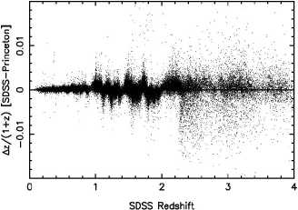
Figure 1: Redshift differences, $\Delta z/(1+z)$, between SDSS and Princeton pipeline reductions. Spectra plotted possess SDSS final-redshifts with high-confidence (zConf$>$0.9) derived via cross-correlation (zstatus=3 or 4). Large differences between redshifts extend to amplitudes of $\pm$5$\times$10^-3 ($\pm$1500 km s^-1). Particularly striking is the sequence of apparent discontinuities in the behaviour of the redshift differences as a function of redshift. Data for 69 915 spectra are included (503 lie outside the y-axis range plotted).

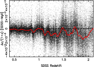
Figure 2: Redshift differences,$\Delta z/(1+z)$, between SDSS redshifts and redshifts derived from the SDSS-determined Mg ii emission line locations. Spectra plotted possess Mg ii emission line SNR$>$10. The solid red line, calculated using a 2001-point running median of the data-points, shows the form of the systematic trends with redshift. Systematic redshift differences of $\simeq$500 km s^-1shifts over small redshift intervals are evident and, over a larger redshift interval, a prominent systematic trend of 2$\times$10^-3 (600 km s^-1) can be seen. Data for 60 190 spectra are included (2101 lie outside the y-axis range plotted).

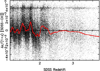
Figure 3: Redshift differences,$\Delta z/(1+z)$, between SDSS redshifts and redshifts derived from the SDSS-determined C iii] emission line locations. Spectra plotted possess C iii] emission line SNR$>$10. The wavelength adopted for the C iii] emission centroid has been chosen to produce, on average, zero-offset for $z$$<$2.2. The solid red line, calculated using a 2001-point running median of the data-points, shows the form of the systematic trends with redshift. Large systematic changes of up to 3$\times$10^-3 (900 km s^-1) over small redshift intervals can be seen. The prominent horizontal ‘feature’ close to $\simeq$4$\times$10^-3 is an artifact resulting from the $\pm$1500 km s^-1velocity interval (about the cross-correlation redshift) within which the SDSS reduction pipeline searches for emission lines. Data for 59 260 spectra are included (2628 lie outside the y-axis range plotted).

4 Master Quasar Template Construction

The generation of the high-SNR quasar template to be used to calculate cross-correlation redshifts begins with a sample of quasars at low redshifts that possess emission line-determined redshifts. A somewhat more involved procedure is then necessary to incorporate additional quasars at higher redshifts into the master template. In this section the recipe for each element of the master template construction are outlined.

4.1 Initial low-redshift quasar template

The narrow forbidden emission lines of [O iii] $\lambda\lambda$4960,5008 are prominent in many quasar spectra with redshifts $z$$<$0.8 and a composite spectrum based on the combination of quasars with redshifts determined via the location of [O iii] emission forms the starting point for the construction of the master quasar template. The $\simeq$19 000 quasars with SDSS redshifts $z$$<$0.85 are searched for the presence of [O iii] emission in a narrow wavelength interval ($\simeq$100 Å) corresponding to the predicted rest-frame location calculated from the SDSS redshift.

A ‘continuum’ is defined using a median filter of 21 pixels and [O iii] $\lambda\lambda$4960,5008 emission then identified using a matched-filter detection scheme applied to a continuum-subtracted version of each spectrum (e.g. ?). [O iii] emission is often broad and frequently exhibits strong asymmetries (?), the small filter-scale adopted for the [O iii] detection is chosen with the aim of isolating narrow, well-defined, peaks that may be present. The filter template consists of two Gaussian components of the same width, centred at 4960.30 Å and 5008.24 Å, with flux ratio 1:3.

Emission features can be identified reliably via detections with relatively low SNR, particularly given the restricted wavelength range searched in each spectrum. However, given the importance of establishing accurate redshifts as the first step in the construction of the composite quasar, the 8542 spectra possessing [O iii] detections with SNR$\geq$8$\sigma$ form the starting point for the template construction.

The recipe used to combine spectra with specified redshifts into a composite is as follows:

• pixels falling within 6.0 Å of the strong night-sky lines at 5578.5 Å and 6301.7 Å are flagged

• pixels without valid SDSS data, determined from the SDSS noise array provided for each spectrum, are flagged

• spectra are shifted to the rest-frame, with the native 69 km s^-1‘pixels’ of the original SDSS spectra retained. The signal from each spectrum is placed onto the master rest-frame wavelength array using a ‘nearest pixel’-scheme, thereby avoiding the need for any rebinning or interpolation

• spectra are normalised using a wavelength interval common to all spectra

• spectra are median-filtered with a window of 61-pixels to define a ‘continuum’. Spectrum pixels falling more than 4.5$\sigma$ below the continuum, along with a grow-radius of two pixels, are flagged, effectively removing wavelengths affected by strong narrow absorption

• the median value of all non-flagged pixels at each rest-frame wavelength is calculated (a minimum of 100 spectra must contribute)

At this point a very high SNR composite quasar spectrum is available, extending down to rest-frame wavelength $\lambda$$\simeq$2300 Å. The [O iii] emission moves beyond the red limit of the SDSS spectra at $z$$>$0.8 and it is necessary to use a cross-correlation scheme, employing a much greater wavelength range of the quasar spectrum, to allow the construction of the master template further into the rest-frame ultra-violet.

4.2 Cross-correlation redshift algorithm

The cross-correlation algorithm is based on a straightforward spatial cross-correlation between an individual quasar spectrum and a high-SNR template spectrum. The key elements of the cross-correlation calculation are i) a conservative choice of the portions of the quasar spectrum to employ in the calculation, avoiding strong emission lines close to the edges of the observed spectrum, and ii) application of an essentially identical ‘window’ to both the individual quasar and template spectra prior to the cross-correlation calculation.

For each quasar spectrum, with its companion error-array, pixels are excluded from the cross-correlation calculation according to a sequence of rules/tests. The first and last valid pixels, where the SDSS spectrum error-array is not set to 0, define the limits of the accessible wavelength range. In the observed-frame:

• the first 25-pixels at each end are excluded

• pixels within 6 Å of each of the strong night-sky emission lines at 5578.5 Å and 6301.5 Å are excluded

• narrow absorption features are identified by examining a continuum-subtracted spectrum. The continuum is defined using a 61-pixel median filter. Pixels that fall more than 4.5$\sigma$ below the continuum are flagged and a grow-radius of 2-pixels then applied. Thus, a single pixel exceeding the threshold results in the exclusion of 5-pixels.

The quasar spectrum is then transformed to the rest-frame using the specified redshift estimate, $z_{init}$. In the rest-frame:

• pixels with $\lambda$$>$7000 Å are excluded

• for $z_{init}$$>$0.38, pixels with $\lambda$$>$6400 Å, i.e. the H$\alpha$ region, are excluded

• for $z_{init}$$<$0.45, pixels with $\lambda$$<$2900 Å, i.e. the Mg ii region, are excluded

• for $z_{init}$$<$1.10, pixels with $\lambda$$<$1975 Å, i.e. the C iii] region, are excluded

• for $z_{init}$$<$4.00, pixels with $\lambda$$<$1675 Å, i.e. the C iv region, are excluded

• pixels with $\lambda$$<$1275 Å, i.e. the N v and Lyman-$\alpha$ lines and the Lyman-$\alpha$ forest, are always excluded.

Following the definition of the restricted wavelength interval over which the quasar spectrum is retained, continua, estimated using a large-scale, 601-pixel, median filter are subtracted from the quasar and the template spectra. Exactly the same wavelength interval is used to estimate the continua subtracted from the quasar and the template spectra.

With continuum-subtracted quasar, $Q_{cs}$, and template, $T_{cs}$, spectra available, the cross-correlation, for lag ”l”, is performed:

$$cc(l)=\frac{\sum_{i}Q_{i}T_{i}/\sigma_{i}^{2}}{\sqrt{{\sum_{i}(Q_{i}/\sigma_{i})^{2}}{\sum_{i}(T_{i}/\sigma_{i})^{2}}}}$$ (1)

where $\sigma_{i}$ is the noise, as provided in the SDSS FITS-files, and the ‘$cs$’ sub-scripts have been omitted for clarity.

A quadratic fit is then made to the array of $cc(l)$ values over the interval $l$=$\pm npix$, with $npix$=100. The fit is then refined, performing quadratic fits to narrower pixel intervals centred on the peak of the previous quadratic fit, with the final fit determined over an interval of $l$=$\pm npix$/5. The output consists of a redshift estimate, $z_{fin}$, and a cross-correlation amplitude, $cc_{max}$, in the range –1$\leq$$cc_{max}$$\leq$1, which parameterises the degree of similarity between the two spectra. Extensive experimentation demonstrates that the requirement $cc_{max}$$\geq$0.2 results in an almost error-free catalogue of cross-correlation redshifts. However, it must be stressed that the use of such a low amplitude is only possible because of the extremely low occurrence of catastrophic redshift mis-identifications resulting from the SDSS spectroscopic pipeline and the subsequent refinements of ??).

4.3 Quasar template extension for redshifts 0.8$<$$z$$\leq$1.6

With the cross-correlation redshift determination procedure in place it is possible to utilise quasars with redshift $z$$>$0.8 to extend the master template. To ensure that the template construction is not adversely affected by the inclusion of spectra with poor SNR, or the presence of broad absorption line (BAL) troughs, the full quasar sample (Section 2) was restricted to those objects satisfying the following criteria:

• SDSS spectrum spectroscopic SNR, SN_R+SN_I $\geq$18.0

• quasar not identified as BAL-quasars by ?) or from our own BAL catalogue (Allen et al. 2010, in preparation)

Application of the criteria reduce the sample by approximately a half, to $\simeq$44 500 spectra. Cross-correlation redshifts are then calculated for 4071 spectra with 0.8$<$$z$$\leq$1.0 according to the prescription of Section 4.2. All spectra with $cc_{max}$$\geq$0.2 and redshifts, 0.8$<$$z$$\leq$1.0, are combined to produce a composite. Then, the original and new composites are combined by taking the average, weighted by the relative number of spectra contributing at each wavelength. The effect is to determine redshifts for quasars using only the wavelength range where the initial (lower-redshift) composite is of high SNR. The procedure is then repeated for intervals of $\Delta z$=0.2 up to redshift $z$=1.6. Table 1 summarises the number of spectra, median absolute magnitudes and wavelength coverage for all of the composites used to generate the final master template spectrum.

The key elements of the scheme are the use of wavelength regions $\geq$1975 Å for the calculation of redshifts of quasars up to $z$=1.6, thereby excluding the C iii] and C iv emission lines. The rest-frame ultra-violet region of interest is shown in Fig. 4.

Figure 4: The master quasar template, plotted as rest-wavelength versus $\lambda$F($\lambda$) (in arbitrary units). The prominent emission line features of H$\alpha$, [O iii] , H$\beta$, [O ii] , Mg ii , C iii] + Si iii] + Al iii and C iv are indicated.

4.4 Luminosity-dependent emission line shifts

Quasar luminosity-dependent systematic effects related to the rest-frame locations of Ca ii absorption, [O ii] , [O iii] and Mg ii emission are at or below the level of 30 km s^-1(Section 6). However, the same is not true when considering the location of the Mg ii emission line and the next prominent emission line complex of C iii] $\lambda$1908, Si iii] $\lambda$1892 and Al iii $\lambda$1857 as one moves further into the ultra-violet. Fig. 5 shows the ratio of the observed-frame centroids of ‘C iii] ’ and Mg ii for quasars in the redshift interval 1.1$<$$z$$<$2.2, where both lines are present in the SDSS spectra. The systematic trend of $\simeq$2$\times$10^-3 in the wavelength ratio as a function of quasar luminosity translates directly into a systematic in $\Delta z$/(1+$z$) where the C iii] emission line region contributes significantly to the cross-correlation signal.

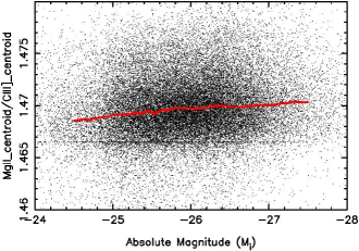
Figure 5: The observed-frame ratio of the centroid wavelengths for Mg ii and C iii] emission lines as a function of the quasar absolute magnitude, $M_{i}$. The quasar sample consists of 42 609 objects with redshifts 1.1$<$$z$$<$2.2. The solid red line, calculated using a 2001-point running median of the data-points, shows the strong systematic trend with quasar luminosity. Data for 1000 spectra lie outside the x-y range plotted.

The luminosity-dependent change in the relative positions of the Mg ii and C iii] emission lines presents a problem when considering the generation of the master quasar template. Indeed, the large systematic means that care is needed when calculating redshifts for a population of quasars with a range of luminosities. Consider the result of cross-correlating a quasar template with a quasar of high luminosity. The C iii] emission in the quasar is at slightly smaller rest-frame wavelength than in the template and the resulting redshift estimate will lie somewhere between redshift estimates based on the locations of the Mg ii and C iii] lines alone. Performing such cross-correlation redshift estimates for a sample of higher redshift quasars and then updating the template with their spectra will have the effect of biasing the profile/location of the Mg ii emission line to smaller wavelengths. The effect is pernicious in that subsequent use of such a template to calculate redshifts for quasars where C iii] is not even visible, will produce biased values because of the systematic change in the profile/location of Mg ii emission and other features in the template. Similar, even larger, luminosity-dependent systematic trends are also present in the relative locations of the C iii] emission complex and the C iv emission line.

The existence of the systematic luminosity-dependent trends in the location of the C iii] and C iv lines means that care must be taken in the definition of the master quasar template.

4.5 Quasar template extension for redshifts 1.6$<$$z$$\leq$2.0

As cross-correlation redshifts are calculated using only rest-frame wavelengths $>$1975 Å for quasars with redshifts $z$$<$1.6, the current master template is free of the luminosity dependent systematics described above. For redshifts $z$$\geq$1.6 it is necessary to use the wavelength range including the C iii] emission complex to increase the SNR of the cross-correlation signal. However, to preserve the form of the composite at wavelengths $>$2000 Å, quasars with redshifts 1.6$\leq$$z$$<$2.0 are incorporated into the template using only wavelengths $<$2000 Å. The master quasar template is extended down to $\lambda$=1275 Å in two redshift slices (Table 1), with the stricture that the quasars in the redshift interval 1.6$\leq$$z$$<$2.0 are not allowed to contribute to the template at wavelengths $\geq$2000 Å.

The result is a final master template in which the form of the spectrum at $\lambda$$\leq$2000 Å is appropriate to a quasar of a particular absolute magnitude ($M_{i}$$\simeq$–26). Given that the SDSS quasars possess a significant spread in absolute magnitude, systematic trends in the redshift determinations using the master quasar template are expected but the amplitude and form of the systematic trends are such that reliable corrections are possible (Section 5) and reliable redshifts can be derived for objects with redshifts up to $z$=4.5.

Table 1: Quasar cross-correlation template definition parameters

Redshift Range	Median $M_{i}$	Number	FD Number	Wavelength Coverage	Redshift Method	Wavelength Contribution
				(Å)		(Å)
0.0–0.4	-22.50	3958	3958	2732–8004	[O iii]	2732–8004
0.4–0.8	-23.86	4584	4584	2136–6550	[O iii]	2136–6550
0.8–1.0	-24.89	4071	4071	1908–5099	Mg ii_cc ($>$1975Å)	1908–5099
1.0–1.2	-25.38	4762	393	1732–4590	Mg ii_cc ($>$1975Å)	1732–4590
1.2–1.4	-25.77	5118	375	1589–4176	Mg ii_cc ($>$1975Å)	1589–4176
1.4–1.6	-26.15	5087	341	1466–3819	Mg ii_cc ($>$1975Å)	1466–3819
1.6–1.8	-26.45	3882	262	1363–3534	Mg ii_cc ($>$1675Å)	1363–2000
1.8–2.0	-26.71	2797	169	1275–3275	Mg ii_cc ($>$1675Å)	1275–2000

5 New Quasar Redshifts

Redshift determinations, in decreasing order of accuracy and increasing quasar redshift, can be obtained using [O iii] emission lines, [O ii] emission lines, cross-correlation including the Mg ii emission line (Mg ii_cc ), cross-correlation including the C iii] emission line complex (C iii]_cc ) and, finally, cross-correlation including the C iv emission line (C iv_cc ). For the cross-correlation results, empirical comparisons of redshifts derived using different rest-frame wavelength regions allow conversion relations to be derived as a function of quasar absolute magnitude and redshift. The goal is to build a redshift ‘ladder’ for quasars of increasing redshift that allows the redshift estimates to be placed on the same underlying systemic reference system. The sub-Sections below consider in turn each step in the ladder.

5.1 [O ii] and [O iii] narrow emission line redshifts

Redshifts for 13291 quasars with redshifts $z$$<$0.84 are available via the detection of [O iii] $\lambda\lambda$4960,5008 emission with a SNR$\geq$6.0$\sigma$ (Section 4.1). Similarly, detection of the [O ii] $\lambda\lambda$3727,3729 emission doublet at a SNR$>$6.0$\sigma$ provides redshift determinations for an additional 3844 quasars, with redshifts $z$$<$1.31.

In the case of [O ii] detections, a single Gaussian, centred at 3728.60 Å, is used. The [O ii] doublet consists of two components centred at 3727.09 Å and 3729.88 Å. The observed component ratio varies from quasar to quasar but is normally in the range 0.8:1–0.9:1, leading to the effective wavelength of 3728.60 Å adopted.

5.2 Cross-correlation redshifts including Mg ii 

Mg ii_cc redshifts are available for a further 12289 quasars with redshifts $z$$\leq$1.10. The minimum rest-frame wavelength involved in the cross-correlation is 1975 Å and systematic offsets relative to the emission line redshifts generated in the previous sub-Section are not predicted or detectable.

In the interval 1.1$<$$z$$<$2.1, the Mg ii_cc redshifts involve rest-frame wavelengths below 1800 Å and the signal is increasingly dominated by the C iii] emission as redshift increases and the Mg ii line shifts into the far red of the SDSS spectra. Additionally, there is also the luminosity-dependent variation in the location of the C iii] emission complex to take into account. The amplitude of the systematic redshift bias is small, only $\simeq$2$\times$10^-4 too large at the highest redshift $z$=2.1.

Taking the Mg ii_cc redshifts and the corresponding Mg ii emission line centroid determinations from the SDSS pipeline allows the dependence of the cross-correlation bias on redshift and absolute magnitude to be quantified. Treating the systematic as separable in redshift and luminosity, a sample of $\simeq$42 000 quasars, in the redshift interval 1.1$<$$z$$<$2.1, shows that linear corrections to the raw cross-correlation redshifts, with slopes of 1.61$\times$10^-4 per unit redshift and 7.2$\times$10^-5 per unit magnitude (reducing the raw redshift estimates as redshift and luminosity increase), bring any residual systematic trends down to the $\simeq$1$\times$10^-5 level. Note that the sense and amplitude of the difference between the raw Mg ii_cc redshifts and the Mg ii emission line centroids are entirely consistent with the existence of the luminosity-dependent emission line shifts and the way that the master quasar template spectrum is constructed (Section 4.4). Corrected Mg ii_cc redshifts are available for 43 728 quasars in the interval 1.1$<$$z$$\leq$2.1.

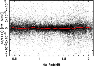
Figure 6: Redshift differences,$\Delta z/(1+z)$, between HW redshifts and redshifts derived from the SDSS-determined Mg ii emission line locations. Spectra plotted possess Mg ii emission line SNR$>$10. The solid red line, calculated using a 2001-point running median of the data-points, demonstrates the complete removal of detectable systematic trends with redshift. Contrast the behaviour with that shown in Fig. 2. Data for 60 120 spectra are included (559 lie outside the y-axis range plotted).

5.3 Cross-correlation redshifts including C iii] 

At redshifts $z$$>$2.1 the Mg ii line no longer contributes to the cross-correlation redshifts and the full effect of the systematic variation in the rest-frame locations of the Mg ii and C iii] emission lines must be taken into account. Fortunately, an empirical determination of the systematic differences between the corrected, un-biased, redshifts derived above and cross-correlation redshifts using only the rest-wavelength region 1675$<$$\lambda$$<$2650 Å, termed C iii]_cc redshifts, is straightforward to make.

The differences between the corrected Mg ii_cc redshifts and raw C iii]_cc redshifts, derived using a maximum rest-frame wavelength of $\lambda$=2650 Å, i.e. excluding the Mg ii emission line, are available for $\simeq$35 000 quasars with 1.1$<$$z$$<$2.0. The difference as a function of quasar absolute magnitude is systematic and well represented by a linear trend; a linear fit has slope 1.67$\times$10^-4, increasing the raw redshifts for increasing bright quasars. Application of the correction removes any detectable systematic effects as a function of absolute magnitude (Fig. 7) or redshift (Fig. 8). The same correction is then applied to C iii]_cc redshifts for 13859 quasars with $z$$>$2.1.

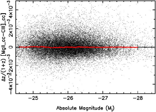
Figure 7: Redshift differences,$\Delta z/(1+z)$, between corrected Mg ii_cc redshifts and corrected C iii]_cc redshifts derived using the C iii] emission line complex alone, as a function of absolute magnitude. The solid red line is a 2001-point running median of the data-points, illustrating the absence of any detectable systematic trends as a function of quasar absolute magnitude. Data for 34 891 spectra are included (119 lie outside the y-axis range plotted).

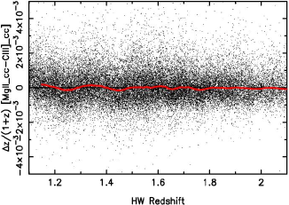
Figure 8: Redshift differences,$\Delta z/(1+z)$, between the corrected Mg ii_cc redshifts and corrected C iii]_cc redshifts derived, as a function of redshift. The solid red line is a 2001-point running median of the data-points showing the absence of any detectable systematic trends as a function of quasar redshift. Data for 35 179 spectra are included (120 lie outside the y-axis range plotted).

5.4 Cross-correlation redshifts including C iv 

The intention throughout is to avoid the use of the rest-frame wavelength region including the C iv emission line, which is known to show large asymmetric variations in shape, and hence of the line centroid. However, for 3274 quasars in the redshift interval 2.1$<$$z$$<$4.5, the cross-correlation signal from the rest-frame $\lambda$$>$1675 Å region is too low to produce a reliable C iii]_cc redshift. For these 3274 quasars a cross-correlation redshift determination employing the rest-frame wavelength interval $\lambda$$>$1275 Å (C iv_cc ) is made.

There is a strong luminosity-dependent bias present due to the systematic variation in the location of the rest-frame C iv emission line centroid. The situation is complicated by the presence, in a large number of quasars, of significant absorption blueward of the C iv emission centroid, which biases the line centroid to the red. To decouple the effects on the C iv emission line of quasar luminosity and the presence of absorption, a sub-sample of $\simeq$25 000 quasars with essentially undetectable absorption blueward of the C iv emission line centroid is defined.

An empirical correction for the systematic luminosity-dependent redshift bias (Fig 9) can then be made in exactly the same way that the C iii]_cc redshifts were referenced to the un-biased system. A two-part linear fit to the absolute magnitude dependence, with slope 6.67$\times$10^-4 for $M_{i}$$<$–27.0 and slope 3.90$\times$10^-4 for $M_{i}$$\geq$–27.0, provides an excellent fit to the systematic trend. The raw C iv_cc redshift estimates are increased for more luminous quasars, reducing systematic redshift differences to undetectable levels. The amplitude of the systematic bias in the raw C iv_cc redshifts is large, a factor of four greater than the C iii] dependence, and the correction results in a substantial reduction in the dispersion between the C iv_cc and un-biased redshift determinations.

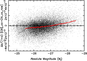
Figure 9: Redshift differences,$\Delta z/(1+z)$, between the corrected HW cross-correlation redshifts and uncorrected C iv_cc redshifts derived including the C iv emission line, as a function of absolute magnitude. The solid red line is a 2001-point running median of the data-points. Data for 34 956 spectra are included (119 lie outside the y-axis range plotted).

Objects with significant absorption blueward of the C iv emission line, many of which are Broad Absorption Line (BAL) quasars, show an extended tail of redshift deviations to high values. A second systematic correction, as a function of the absorption equivalent width (AEW) is then made, using the differences between the corrected C iii]_cc redshifts and the absolute magnitude corrected C iv_cc values for $\simeq$38 000 quasars. The actual correction applied is based on the empirically-determined median $\Delta z/(1+z)$ versus AEW relation but the amplitude of the well-determined correction is closely reproduced by a linear fit with slope –2.5$\times$10^-5 over the 0–200 range of AEW used. The additional quasar-to-quasar dispersion in redshift at large AEW is significant but only 574 quasars with AEW$>$20 in the final catalogue possess C iv_cc redshifts.

Table 2 summarises the redshift and absolute magnitude dependent corrections made to the redshifts from the different estimation schemes in the ladder.

Table 2: Systematic redshift corrections

Redshift Method	Number	Redshift Interval	Redshift Correction	$M_{i}$ Correction
			($|\Delta z/(1+z)|$ per unit $z$)	($|\Delta z/(1+z)|$ per unit $M_{i}$)
[O iii]	13291	$<$0.84	–	–
[O ii]	3844	$<$1.35	–	–
Mg ii_cc	12289	$<$1.1	–	–
Mg ii_cc	43728	1.1–2.1	1.61$\times$10-4	7.2$\times$10-5
C iii]_cc	13859	1.1–4.1	–	1.67$\times$10-4
C iv_cc	3274	1.5–5.5	–	6.67$\times$10-4 $<$–27.0
C iv_cc			–	3.90$\times$10-4 $\geq$–27.0

5.5 Additional redshifts

Redshifts for an additional 124 quasars are available, although one of the strict criterion described above is not satisfied, e.g. SNR$<$6.0$\sigma$ for an emission line detection, or $cc_{max}$$<$0.2. These redshifts are included in the catalogue but are highlighted by the inclusion of a special status flag.

Finally, the emission line detection and cross-correlation schemes fail to provide reliable redshift estimates for 1256 quasars. These objects consist primarily of a mix of pathological spectra, including extreme BAL quasars, and spectra of very low SNR. The objects are included in the redshift catalogue for completeness, with redshifts and redshift errors taken from the Schneider et al. catalogues (??) and the spectro1d pipeline for DR6. Again, the source of the redshifts is indicated in the catalogue via a status flag.

6 Systemic Redshifts and Redshift Uncertainties

Section 5 describes the scheme adopted to obtain redshifts using the most reliable estimation procedure for each quasar. Redshifts are referenced to the zero-point provided by the location of the [O iii]  $\lambda\lambda$4960,5008 emission lines. The goal is to reduce systematic errors in $\Delta z/(1+z)$ to the level of $\leq$1$\times$10^-4 (30 km s^-1) per unit redshift and $\leq$2.5$\times$10^-5 (8 km s^-1) per unit absolute magnitude. In this section the question of referencing the [O iii] emission line redshifts to the systemic system defined by the quasar host galaxies is considered. Starting with the comparison of absorption line and [O iii] emission redshifts, the uncertainties in redshift estimates arising from both the intrinsic quasar-to-quasar variation and the reproducibility of the determinations for each technique in the ladder are quantified.

6.1 [O iii] and host galaxy systemic redshifts

Redshift estimates based on the detection of photospheric absorption from stars in the spatially averaged spectrum of the quasar host galaxy might be expected to provide a close to ‘ideal’ systemic redshift. Given the nature of the SDSS spectra, coupled with the large luminosity of the quasars at rest-frame optical and near-ultra-violet wavelengths, detection of photospheric absorption is not possible for the majority of objects. However, a direct comparison of redshifts derived from photospheric Ca ii $\lambda\lambda$3934.8,3969.6 and [O iii] emission is possible for a sample of objects with redshifts $z$$<$0.4. Generating a catalogue of Ca ii absorption detections with SNR$>$6$\sigma$, matched to quasars with [O iii] detections in the redshift interval 0.2$\leq$$z$$\leq$0.4, produces 825 quasars. Restricting the sample to objects that satisfy the luminosity-criterion for inclusion in the Schneider et al. SDSS quasar compilations, results in 615 quasars with absolute magnitudes covering the full range –24.0$<$$M_{i}$$<$–22.0. Composite spectra with median $M_{i}$=–22.2 and –22.6 possess both Ca ii absorption and [O iii] emission at high SNR.

Measuring the centroid of the strong Ca ii K-line at 3934.8Å (Ca ii H is blended with H$\epsilon$ absorption, producing a shift to longer wavelengths) and the centroid of the [O iii] $\lambda\lambda$4960.30,5008.24 emission, measured above the 50 per cent peak-height level, shows that the [O iii] emission is shifted by 45$\pm$5 km s^-1to the blue, with no detectable dependence on luminosity. The offset determined from the composite spectra is in good agreement with the results of (?) and the distribution of individual Ca ii and [O iii] redshift-differences for the 615 objects contributing to the composites. The median redshift difference for the sample corresponds to a velocity shift of 38$\pm$9 km s^-1blueward for [O iii] relative to Ca ii . We therefore correct all redshifts by a 45 km s^-1shift to the red to bring the zero-point into coincidence with the system defined by the Ca ii K-line.

After correcting for the contribution of the redshift reproducibility ($\sigma_{repro}$=2.1$\times$10^-4, calculated using multiple spectra (Section 2)) in estimating the Ca ii redshifts, the empirically determined quasar-to-quasar scatter of [O iii] redshifts about the Ca ii absorber redshifts is $\sigma_{intrin}$=3.5$\times$10^-4.

6.2 [O iii] and [O ii] emission line redshifts

A similar comparison can be made between the [O iii] and [O ii] emission line derived redshifts for the more than 7500 quasars, redshifts $z$$<$0.8, with both [O iii] and [O ii] emission line detections. A small systematic velocity offset is present, with the [O ii] derived redshifts 24$\pm 5$ km s^-1redward of the [O iii] derived redshifts. Thus, relative to the systemic reference defined by the Ca ii K absorption, the offsets are 21$\pm$5 km s^-1blueward for [O ii] and 45$\pm$5 km s^-1blueward for [O iii] , in excellent agreement with previous work (?, e.g.).

Comparison of 1378 (1103) spectrum pairs results in median errors of 5$\times$10^-5 and 1.4$\times$10^-4 in the reproducibility of $\Delta z$/(1+$z$) for [O iii] and [O ii] respectively. The smaller error for [O iii] results from the typically higher SNR of the emission compared to the [O ii] line.

Systematic trends, derived from linear fits to the redshift differences between [O iii] and [O ii] redshifts, are $\Delta z$/(1+$z$)=2.1$\times$10^-5 per magnitude and $\Delta z$/(1+$z$)=5.9$\times$10^-5 per unit redshift. The sense is that redshifts derived from the [O iii] emission lines become systematically smaller for objects with higher luminosities(redshifts). The luminosity-dependent systematic is stronger than for redshift given the dynamic ranges of the variables present in the sample. The trend is consistent with an increasing degree of blue-asymmetry present in the [O iii] emission lines at increasing quasar luminosity. The effect is, however, small, amounting to a maximum of $\pm$4.5$\times$10^-5, or, $\pm$14 km s^-1, about the mean relation for the sample.

The empirically determined quasar-to-quasar rms-scatter of the individual [O ii] redshifts about the [O iii] redshifts is $\sigma_{intrin}$=1.0$\times$10^-4 (30 km s^-1).

6.3 [O iii] and Mg ii_cc redshifts

[O iii] emission line redshifts compared to Mg ii_cc redshifts, calculated excluding the [O iii] emission lines from the quasar template, for $\simeq$12 500 quasars with [O iii] emission line reshifts shows an undetectable offset, median $|\Delta z$/(1+$z$)$|$$<$10^-5. Systematic trends, from linear fits to the redshift differences, in sense [O iii] - Mg ii_cc redshifts, are $\Delta z$/(1+$z$)=+1$\times$10^-5 per magnitude and $\Delta z$/(1+$z$)=-1.1$\times$10^-4 per unit redshift. Both luminosity and redshift parameterisations lead to systematics of at most $\pm$3$\times$10^-5 (10 km s^-1), for the dynamic ranges present in the sample, more than an order of magnitude below the uncertainties in the individual [O iii] redshifts (Section 6.1). The sense and amplitude of the small systematic is consistent with the results from the [O iii] to [O ii] emission line comparison (Section 6.2) and is again almost certainly due to the increasing degree of blue-asymmetry present in the [O iii] emission lines at increasing quasar luminosity. The comparison shows that the Mg ii_cc redshifts are tied to the reference [O iii] emission line redshifts to very high accuracy and that any systematics present are at most 10^-4 in $\Delta z$/(1+$z$), or 30 km s^-1in velocity.

The empirically determined quasar-to-quasar scatter of the individual Mg ii_cc redshifts about the [O iii] redshifts is $\sigma_{intrin}$=2.5$\times$10^-4 or 75 km s^-1, which represents an improvement of a factor of $\sim$3 compared to careful determinations of the Mg ii emission line location (e.g. ?).

Table 3: Redshift uncertainties

Redshift Method	Number	Redshift Interval	Reproducibility	Population rms	Cumulative Population rms
			($\Delta z/(1+z)$)	($\Delta z/(1+z)$)	($\Delta z/(1+z)$)
Ca ii K	–	0.2–0.4	2.1$\times$10-4	–	–
[O iii]	13291	$<$0.84	5$\times$10-5	3.5$\times$10-4	3.5$\times$10-4
[O ii]	3844	$<$1.35	1.4$\times$10-4	1.0$\times$10-4	3.65$\times$10-4
Mg ii_cc	12289	$<$1.1	1.4$\times$10-4	2.5$\times$10-4	4.3$\times$10-4
Mg ii_cc	43728	1.1–2.1	3.6$\times$10-4	2.5$\times$10-4	4.3$\times$10-4
C iii]_cc	13859	1.1–4.1	6.5$\times$10-4	2.5$\times$10-4	4.3$\times$10-4
C iv_cc	2700	1.5–5.5	5.1$\times$10-4	8.0$\times$10-4	9.1$\times$10-4
C iv_cc + AEW	574			1.0$\times$10-3	1.4$\times$10-3
extra_cc	124	0.5–4.5	6.0$\times$10-4	3.0$\times$10-4	3.5$\times$10-4
SDSS	1256	0.3–5.5	as per SDSS	–

6.4 Mg ii_cc and C iii]_cc redshifts

The luminosity-dependent correction to bring the Mg ii_cc and C iii]_cc redshifts into coincidence is highly successful, as evidenced by Fig. 7 and Fig. 8.

After allowing for the uncertainty in the determination of the Mg ii_cc and C iii]_cc redshifts due to the limited SNR of the SDSS spectra there is no evidence for an additional quasar-to-quasar redshift scatter associated with the use of the C iii] emission line region alone.

6.5 C iii]_cc and C iv_cc redshifts

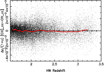
Figure 10: Redshift differences,$\Delta z/(1+z)$, between the corrected C iii]_cc redshifts and corrected C iv_cc redshifts derived using the C iv emission line complex alone, as a function of redshift. Data for 25 008 quasars with AEW$\leq$20 are included (60 lie outside the y-axis range plotted). The solid red line is a 2001-point running median of the data-points. The offset between the two redshift estimators is minimal except for the systematic ‘dip’ centred at $z$$\simeq$2.8, coincident with the significant drop in detection efficiency for non-BAL quasars in the SDSS.

The diversity of the form of the C iv emission line has been known through many studies going back decades. The removal of the systematic quasar luminosity-dependent behaviour, amounting to $\simeq$650 km s^-1(over four magnitudes in quasar absolute magnitude), improves C iv_cc redshifts considerably. However, even for quasars with small AEW values the empirically determined quasar-to-quasar scatter of the individual C iv_cc redshifts about the C iii]_cc redshifts is $\sigma_{intrin}$=8.0$\times$10^-4. The situation is much worse for quasars with significant absorption blueward of the C iv emission line centroid. The systematic correction applied reaches a full 5$\times$10^-3 for the most affected quasars and the dispersion at fixed AEW value adds an additional rms-scatter of $\sigma_{intrin}$=1$\times$10^-3. The number of quasars with large AEW values where only C iv_cc redshifts are available is small, just 574 objects, but the associated redshift uncertainty is accordingly large.

Fig. 10 shows the redshift differences between the corrected C iii]_cc and corrected C iv_cc redshifts for 25 008 quasars with only modest absorption (AEW$\leq$20) blueward of the C iv emission line. The small amplitude of the systematic differences illustrates the success of the statistical correction to the initial C iv_cc redshifts. However, the systematic negative trend centred on $z$$\simeq$2.8, which reaches $\simeq$–1.8$\times$10^-4 (55 km s^-1), illustrates the limitations of the correction. The SDSS quasar selection experiences a dramatic drop in efficiency over the interval $z$$\simeq$2.7–2.9 that is much greater for non-BAL quasars than for BAL quasars. Thus, the overall number of quasars drops significantly, while the BAL-fraction increases significantly. There are only 13 quasars with 2.7$\leq$$z$$\leq$2.9 and with AEW$\leq$20, in the final catalogue but a systematic of at least –2$\times$10^-4 may well also be present among the 574 quasars with C iv_cc redshifts and AEW$>$20

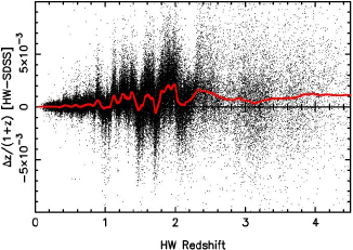
Figure 11: Redshift differences,$\Delta z/(1+z)$, between the final HW-redshifts and SDSS-redshifts, as a function of redshift. Note the large range on the y-axis. Data for 90 409 quasars are included (1355 lie outside the y-axis range plotted).

6.6 Summary

All redshift estimates, except those taken direct from the SDSS, have been increased by 45 km s^-1(Section 6.1) to bring the [O iii] emission line based estimates onto the systemic system defined by the Ca ii K absorption.

Based on the large sample of repeat spectra, the internal reproducibility of the new cross-correlation redshifts represent an improvement of more than a factor 2 over the SDSS redshift values. The reproducibility of the new redshifts is indistinguishable from that for the Princeton redshift values up to redshift $z$$\simeq$1.6. At higher redshifts the Princeton algorithm employs more information, via inclusion of the C iv emission line region at $\lambda$$<$1675 Å, and results in significantly better reproducibility for redshifts $z$$>$2.0 than in the scheme presented here. However, the large quasar-to-quasar variation contributing to the redshift uncertainty (Table 3) means that differences in the internal reproducibility are not a critical factor for the redshifts in the final catalogue.

Table 3 summarises the uncertainties for the different redshift estimates. Accurate redshift reproducibility estimates are available for all quasars, based on emission line SNR or $cc_{max}$ value, and are incorporated in the redshift errors included in Table 4. To provide an indication of the relative contributions of the internal and quasar-to-quasar uncertainties, Col. 4 of Table 3 lists the median internal error for each redshift estimate. Col. 5 gives the quasar-to-quasar error. The quasar-to-quasar errors, working from the chosen Ca ii absorption reference, have been added in quadrature to produce the cumulative quasar-to-quasar uncertainties in Col. 7.

7 Quasars with detections in FIRST

The procedures described in Sections 5 and 6 reduce systematic redshift errors as a function of redshift and absolute magnitude by more than order of magnitude compared to the publicly available SDSS redshifts. However, a further significant reduction in the remaining relatively large quasar-to-quasar uncertainties will require a detailed investigation of the spectral energy distribution (SED) dependent changes in the properties of the most prominent emission lines (which dominate the redshift determinations). Such an investigation is beyond the scope of this paper but it is relatively straightforward to consider systematic redshift differences that correlate with the detection of SDSS quasars in the Faint Images of the Radio Sky at Twenty centimetres (FIRST, ?).

For redshifts $z$$<$1.1, the systematic differences between the populations of FIRST-detected (FD) and not-FIRST-detected (nFD) quasars with Mg ii_cc cross-correlation redshifts are at the $\Delta z$/(1+$z$)$\leq$10^-4 level. However, for redshifts $z$$>$1.1, once the C iii] +Si iii] +Al iii emission line complex contributes to the redshift determination, systematic differences become increasingly evident, reaching an amplitude of nearly $\Delta z$/(1+$z$)=2$\times$10^-3 (600 km s^-1) at redshifts $z$$\ga$4.

The origin of the redshift differences is primarily a systematic change in the ratio of the C iii] and Si iii] emission lines in the FD- and nFD-populations. The line ratio change results in a shift in the centroid of the blended line; Si iii] is weaker in the FD-detected quasars and the blended line centroid moves redward. The Mg ii_cc redshifts for the FD quasars are thus too large.

Based on the prescription of ?) for matching SDSS quasars to the FIRST survey there are 4326 FD-quasars with $z$$>$1.1 in the DR6 quasar catalogue. The small fraction (7 per cent) of FD-quasars, combined with the low amplitude of the systematic redshift differences, means that the inclusion of FD-detected quasars in construction of the master template results in changes to cross-correlation redshifts of $\Delta z$/(1+$z$)$<$10^-4. However, generation of an individual template for the FD-quasars results in a quasar template with significant differences in the form of the C iii] +Si iii] +Al iii emission line complex (Fig. 12).

Construction of the new FD-quasar template proceeds in an identical fashion to that described in Section 4 but the individual quasars used differ. For redshifts $z$$<$1.0 the same quasars used to generate the master quasar template are employed, whereas, at redshifts $z$$>1.0$, only FD-quasars are used, with the minimum number of spectra required to generate a composite in a redshift slice reduced from 100 to 50 (Section 4). The number of quasars contributing at each redshift interval is given in Col. 4 of Table 1. As evident from Fig. 12, the form of the C iii] +Si iii] +Al iii emission line complex differs between the master- and FD-quasar-templates. The size of the empirical transformations necessary to bring the FD-quasar redshift estimates onto the reference system, in which the Mg ii emission line centroid does not vary, with either redshift or absolute magnitude, are significantly reduced compared to the quasar population as a whole.

For redshifts 1.1$\leq$$z$$<$2.1 a reduction of $\Delta z/(1+z)$=1.42$\times$10^-4 in the Mg ii_cc redshifts, independent of redshift and absolute magnitude, is necessary. For C iii]_cc redshifts an absolute magnitude dependent correction of 4.19$\times$10^-5, in the opposite sense to that for the master template, is required, i.e. for bright quasars the C iii]_cc redshifts are reduced. However, given the $\simeq$4 mag dynamic range of the quasar sample, the maximum correction for any quasar is $\Delta z/(1+z)$$\la$10^-4. For the small number of quasars where it is necessary to employ the C iv emission line, the C iv_cc redshifts require a correction with slope 3.44$\times$10^-4, in the same sense as the larger correction necessary for the master template, i.e. for bright quasars the C iv_cc redshifts are increased (Fig. 9).

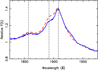
Figure 12: Rest-frame spectra including the prominent emission line complex of C iii] $\lambda$1908, Si iii] $\lambda$1892 and Al iii $\lambda$1857, for the master quasar template (red dash-dot line) and the FIRST-detected template (blue solid line). The reference wavelengths of the three emission line species are indicated by the vertical dotted lines. The significant difference in flux coincident with the location of the Si iii] $\lambda$1892 is evident.

Table 4: Quasar redshift catalogue. The full table is available in the electronic version of the journal.

Name	RA	Dec	$z$	$\sigma_{z}$	FIRST	$z$ Alternate	Plate	MJD	Fibre	Code
	J2000 (deg)	J2000 (deg)
SDSS J000006.53+003055.2	0.02723	0.51534	1.823154	0.001025	-1	-999.0	685	52203	467	3
SDSS J000008.13+001634.6	0.03390	0.27630	1.836332	0.000614	-1	-999.0	685	52203	470	3
SDSS J000009.26+151754.5	0.03860	15.29848	1.197436	0.000369	0	1.200035	751	52251	354	2
SDSS J000009.38+135618.4	0.03909	13.93845	2.240486	0.001468	0	2.240486	750	52235	82	7
SDSS J000009.42-102751.9	0.03927	-10.46443	1.851731	0.000966	-1	-999.0	650	52143	199	3
SDSS J000011.41+145545.6	0.04755	14.92935	0.460127	0.000357	0	-999.0	750	52235	499	1
SDSS J000011.96+000225.3	0.04984	0.04036	0.478321	0.000358	-1	-999.0	387	51791	200	1
SDSS J000012.25-003220.5	0.05108	-0.53905	1.437047	0.000697	-1	-999.0	1091	52902	129	3
SDSS J000013.14+141034.6	0.05479	14.17630	0.949947	0.000521	0	-999.0	750	52235	98	3
SDSS J000013.80-005446.8	0.05751	-0.91300	1.840606	0.000789	-1	-999.0	1091	52902	108	3

Table 5: Quasar cross-correlation templates. The full table is available in the electronic version of the journal.

Wavelength	Relative Flux	Number	Relative Flux	Number
(Å)	(per unit wavelength)		(per unit wavelength)
1275.26	8.130	179	-999.0	0
1275.56	7.582	186	-999.0	0
1275.85	7.845	191	-999.0	0
1276.15	7.780	196	-999.0	0
1276.44	7.673	204	-999.0	0
1276.73	7.682	212	-999.0	0
1277.03	7.730	219	-999.0	0
1277.32	7.862	229	-999.0	0
1277.61	7.644	234	-999.0	0
1277.91	7.755	247	-999.0	0

8 The Redshift Catalogue

Table 4 includes redshifts and error estimates for 91 665 quasars. Col. 1: is the SDSS coordinate object name, taken from the SDSS DR7 Legacy Release whenever available. Cols. 2 and 3 give the object J2000 right ascension and declination in decimal degrees. The redshift and redshift error are given in Cols. 4 and 5 respectively. Col. 6 provides a code specifying the FIRST-detection (FD) status of the quasar (–1: not detected, 0: outside FIRST footprint, 1: detected). Col. 7, alternate redshift for quasars with Col. 6 detection code =0 (derived using the FD-quasar template) and =1 (derived using the master quasar template). The alternate redshift is assigned a value of ‘–999.0’ for quasars with Col. 6 detection code =–1. Col. 8 specifies the origin of the redshift estimate via a numerical code (1: [O iii] , 2: [O ii] , 3: Mg ii_cc , 4: C iii]_cc , 5: C iv_cc , 6: extra_cc, 7: SDSS). The SDSS spectrum from which the redshift estimate is derived is specified via the spectroscopic plate number. modified Julian date of observation and fibre number in Cols. 9, 10 and 11 respectively. The redshifts are given to six decimal places but, as evident from the size of the associated errors, the accuracy for individual objects is two orders of magnitude larger. The high level of precision is retained to avoid quantisation when comparing different redshift estimates specified to only four decimal places.

The provision of alternate redshifts for FD-quasars and quasars whose FIRST detection status is unclear, allows the use of an appropriate redshift by researchers with particular definitions of ‘radio’-quasar subsamples and/or additional radio-observations for quasars outside the current FIRST footprint. The primary (Col. 4) and alternate (Col. 7) redshifts differ only when the primary redshift is derived from cross-correlation (with one of the two quasar templates) and has a value $z$$>$1.1.

Two quasars, SDSS J134415.75+331719.1 and SDSS J142507.32+323137.4, exhibit distinctive double-peaked narrow emission. In both cases, the redshift corresponding to the higher velocity system is included in the table.

The majority of researchers will be interested in the combined redshift error (Col. 5) arising from the limited SNR of the SDSS spectra and intrinsic variation from quasar-to-quasar. However, the internal contribution can be recovered straightforwardly via use of the amplitude of the quasar-to-quasar errors listed in Table 3.

Table 5 presents the master quasar templates used to estimate the cross-correlation redshifts. Col. 1 lists the rest-frame wavelength (Å). Cols. 2, and 3 include the relative flux (per unit wavelength) and the number of spectra contributing for the master template, while Cols. 4 and 5 provide the same information for the FD-quasar template. The FD-quasar template does not extend quite as far to the blue and the flux column contains entries of ‘–999.0’ for wavelengths $\lambda$$<$1296.2 Å.

While the spectra should prove of use in the context of redshift estimation, the templates are not suitable for studies of quasar spectral energy distributions, where care must be taken in defining the large-scale shape of such composite spectra.

9 Discussion

The approach adopted in this paper to the question of deriving redshifts with a common zero-point over an extended dynamic range in redshift, and hence involving disjoint spectral wavelength coverage, differs from that normally employed. The majority of studies to date have focussed on the parameterisation of the rest-frame centroid differences between the strongest emission lines present in the quasar spectra (e.g. Appendix A of ?, for a recent example). Use of the cross-correlation redshifts directly, bypasses many of the difficulties associated in providing reliable, reproducible, parameterisations of low SNR, asymmetric, often blended, emission lines present on ‘continua’ that also show significant variation from quasar to quasar. The resultant quasar-to-quasar dispersion and the internal reproducibility of the new HW-redshifts represent significant improvements over even the most careful studies utilising individual emission features.

Systematic, luminosity-dependent relative emission line shifts have not featured in many previous studies of the quasar population. In part, the lack of such work may reflect the difficulty of performing such studies prior to the availability of the more recent SDSS Data Releases. An exception is the work of ?) who find a clear relationship between emission line centroid shifts, of exactly the type discussed here, and emission line equivalent width. ?) note that the line equivalent width is directly related to quasar absolute magnitude via the Baldwin Effect (?).

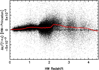
Figure 13: Redshift differences,$\Delta z/(1+z)$, between the final HW-redshifts and Princeton redshifts, as a function of redshift. Note the large range on the y-axis. Data for 90 979 quasars are included (1306 lie outside the y-axis range plotted).

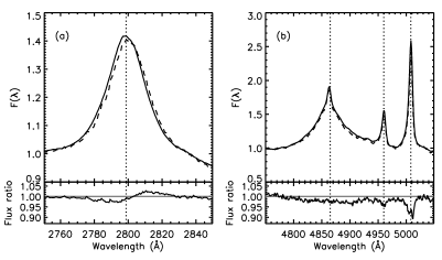
Figure 14: Rest-frame spectra of the new quasar composite compared to that of ?). Panel (a) shows the prominent emission line of Mg ii $\lambda\lambda$2796.35,2803.53, with the new quasar composite (solid line) and the ?) composite (dashed line). The lower plot shows the ratio ?)/new. The vertical dotted line indicates the wavelength 2798.75 Å, derived from the Mg ii components in the ratio 2:1. The significantly bluer location of Mg ii emission in the new composite is evident. Panel (b) shows the same information for the rest-frame wavelength region including H$\beta$ and [O iii] $\lambda\lambda$4960,5008. The vertical dotted lines indicate the rest-frame wavelengths of 4862.68 4960.30 and 5008.24 Å for H$\beta$ and [O iii] . While the new composite possesses slightly stronger [O iii] emission there is no evidence for any detectable offset in the emission line locations of H$\beta$ or [O iii] .

9.1 Comparison with Princeton redshifts and the ?) quasar template

Operationally, it is found that straightforward systematic corrections to quasar redshift estimates, as a function of quasar absolute magnitude, reduce the systematic trends as a function of redshift (absolute magnitude) to $<$30 km s^-1per unit redshift ($<$10 km s^-1per magnitude). Internal reproducibility represents a factor $>$2 improvement over the SDSS redshift determinations. The results presented above, combined with the form of the differences between the Princeton and SDSS redshifts (Section 3), show that the origin of a significant proportion of the improvements achieved are due to differences in the cross-correlation procedure/algorithm employed. However, comparison of the new HW-redshifts with the Princeton determinations (Fig. 13) still shows large ($\simeq$600 km s^-1at $z$$\simeq$2.2) systematic differences.

The two evident ‘jumps’ in the relationship between the HW- and SDSS- estimates occur as cross-correlation redshifts including the Mg ii $\lambda$2799 emission line become important (at $z$$\sim$0.8) and where Mg ii moves beyond the red limit of the SDSS spectra (at $z$$\simeq$2.1). The behaviour can be traced directly to differences in the new quasar template and that of ?). Fig. 14b shows the excellent agreement between the composites at optical wavelengths where emission lines, including H$\beta$ and [O iii] $\lambda\lambda$4960,5008, dominate the redshift determinations (either directly, via emission line locations, or, through the contribution of emission lines to the cross-correlation signal). In contrast, Fig. 14a, illustrates the significant difference in the location of the Mg ii $\lambda$2799 emission line in the two composites. At the accuracy levels of interest, absolute wavelength ‘centroids’ of broad emission lines in quasar spectra are dominated by the particular scheme used to define the associated ‘continuum’ and the height above the continuum used to define the ‘line’. However, the centroid of the portion of the Mg ii emission line above half the peak height is 1.2$\pm$0.1 Å bluer in the HW-template compared to the ?) template. The line centroid moves redward as increasingly large fractions of the line wings are included but at the half peak height level the HW-template line centroid is only 0.4$\pm 0.1$ Å ($\simeq$45 km s^-1) redward of the rest-frame reference value of 2798.75 Å, derived from the Mg ii components in the ratio 2:1.

The strongest ‘jump’ in the relation between the HW- and Princeton-redshifts in Fig. 13, at $z$$\simeq$2.2, derives fundamentally from the large systematic trends in the ratio of Mg ii to ‘C iii] ’ emission line locations as a function of quasar absolute magnitude (Fig. 5). The origin of the effect is primarily the change in the ratio of C iii] $\lambda$1908 to Si iii] $\lambda$1892 (see Fig. 12 for illustration in the context of FIRST-detected quasars). A direct comparison of the HW-template and ?) template is somewhat misleading because the HW-redshifts are derived only following the significant absolute magnitude dependent corrections. However, using any sensible definition of the emission line, the C iii] + Si iii] blend is significantly bluer in the HW-template than in the ?) composite, producing the increase in the HW-redshifts at $z$$\simeq$2.2. The Princeton redshifts then become progressively closer to the HW-redshifts as the C iv emission line (with its well-established increasing blue asymmetry at increasing quasar luminosity) dominates the Princeton determinations at higher redshifts. Recall though, that the C iv emission region does not contribute to the HW-redshifts, except in a very small percentage of quasars.

9.2 Associated C iv and Mg ii absorbers as quasar redshift diagnostics

The availability of the large SDSS quasar catalogues have stimulated new investigations into the physical origin of associated absorbers, particularly those evident through the presence of C iv and Mg ii absorption (e.g. ???). A pre-requisite for such investigations is an estimate of the systemic quasar redshifts. Given the large intrinsic variation in the properties of the C iv emission line and the relative invariance of the Mg ii emission line centroid, redshifts based on the location of the Mg ii emission line are often employed in studies of both associated C iv and Mg ii absorbers in quasars with redshifts $z$$\leq$2.1.

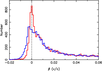
Figure 15: Observed frequency distribution of redshift differences, $\beta$=$v/c$, for $\simeq$23 800 C iv absorbers using both SDSS- (blue) and HW-redshifts (red) for quasars with redshifts 1.55$<$$z$$<$3.5. The HW-redshift-based histogram shows a much higher, better defined, peak, centred close to $\beta$$\simeq$0 and a greatly reduced population of absorbers with positive $\beta$ values (i.e. $z_{abs}$$>$$z_{qso}$). The centroid of the $\beta$$\simeq$0 component for the HW-redshifts shows no detectable shift over the entire redshift range of the quasars, 1.55$<$$z$$<$3.5.

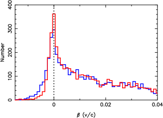
Figure 16: Observed frequency distribution of redshift differences, $\beta$=$v/c$, for $\simeq$8750 Mg ii absorbers using both SDSS- (blue) and HW-redshifts (red) for quasars with redshifts 0.45$<$$z$$<$2.1. The HW-redshift-based histogram shows a higher, better defined, peak, centred close to $\beta$$\simeq$0 and a significantly reduced population of absorbers with positive $\beta$ values (i.e. $z_{abs}$$>$$z_{qso}$). The centroid of the $\beta$$\simeq$0 component for the HW-redshifts shows no detectable shift over the entire redshift range of the quasars, 0.45$<$$z$$<$2.1.

Both Mg ii and C iv absorber catalogues are available from our investigation of absorber populations in SDSS quasars (e.g. ?). Strong narrow absorbers are flagged and ‘removed’ from the quasar spectra prior to the calculation of the cross-correlation redshift determinations (Section 4). The new HW-quasar redshifts are thus essentially independent of the presence of individual absorbers and a comparison of associated absorbers velocity distributions, using both SDSS- and HW-redshifts, provides a powerful test of the redshift accuracy in an astrophysical context of considerable current interest. Fig. 15 shows the observed distribution of redshift differences , $\beta$=$v/c$, for $\simeq$23 800 C iv absorbers using both SDSS- and HW-redshifts for quasars with redshifts 1.55$<$$z$$<$3.5. The differences in the distributions are striking, with the HW-redshift-based histogram showing a much higher peak at $\beta$$\simeq$0 and a greatly reduced population of positive $\beta$ values (i.e. $z_{abs}$$>$$z_{qso}$). The centroid of the $\beta$$\simeq$0 component shows no detectable shift over the entire redshift range of the quasars, 1.55$<$$z$$<$3.5.

Fig. 16 shows the equivalent distribution of redshift differences, for $\simeq$8750 Mg ii absorbers using both SDSS- and HW-redshifts for quasars with redshifts 0.45$<$$z$$<$2.1. The differences between the SDSS- and HW-redshifts at $z$$<$2.1 are significantly smaller than for the quasars included in the C iv absorber sample. However, similar behaviour is evident to that seen in the C iv absorbers, the $\beta$$\simeq$0 peak is significantly better defined using the HW-redshifts and the population of redshifted absorbers with positive $\beta$ greatly reduced. A more detailed consideration of the distribution of the Mg ii absorber redshifts leads to an improved parameterisation of the various constituent absorber populations (?).

To summarise, the distributions of the C iv and Mg ii associated absorber populations provide independent confirmation of the veracity of the new HW-redshifts. While beyond the scope of the present paper, investigations of associated absorber populations are in hand using the full SDSS DR7 Legacy Release spectroscopic database.

10 conclusions

A systematic investigation of the relationship between different redshift estimation schemes for more than 91 000 quasars in the Sloan Digital Sky Survey (SDSS) Data Release 6 (DR6) is presented. Empirical relationships between redshifts based on i) Ca ii H & K host galaxy absorption, ii) quasar [O ii] $\lambda$3728, iii) [O iii] $\lambda\lambda$4960,5008 emission, and iv) cross-correlation (with a master quasar template) that includes, at increasing quasar redshift, the prominent Mg ii $\lambda$2799, C iii] $\lambda$1908 and C iv $\lambda$1549 emission lines, are established as a function of quasar redshift and luminosity. New redshifts in the resulting catalogue possess systematic biases a factor of $\simeq$20 lower compared to the SDSS redshift values; systematic effects are reduced to the level of $\Delta z/(1+z)$$\leq$10^-4 (30 km s^-1) per unit redshift, or $\leq$2.5$\times$10^-5 per unit absolute magnitude.

It is important to realise that there will be systematic redshift trends present as a function of the quasar SEDs and the specific example of FIRST-detected quasars (Section 7) provides an example, related to the radio-properties of the quasar SEDs. One of the primary motivations of this work is to facilitate further studies of SED-dependent systematic emission line properties, working from redshift estimates whose properties as a function of redshift and absolute magnitude are well understood.

Equally important as the new redshift determinations, well-determined empirical estimates of the quasar-to-quasar dispersion in redshifts are available for each method of redshift estimation and a combined internal+population uncertainty is provided for every quasar in the catalogue.

The improved redshifts and their associated errors have wide applicability in areas such as quasar absorption outflows, quasar clustering, quasar-galaxy clustering and proximity-effect determinations.

Bibliography

- Abazajian K. N., et al., 2009, ApJS, 182, 543
- Adelman-McCarthy J. K., et al., 2007, ApJS, 172, 634
- Adelman-McCarthy J. K., et al., 2008, ApJS, 175, 297
- Bajtlik S., Duncan R. C., Ostriker J. P., 1988, ApJ, 327, 570
- Baldwin J. A., 1977, ApJ, 214, 679
- Becker R. H., White R. L., Helfand D. J., 1995, ApJ, 450, 559
- Boroson T., 2005, AJ, 130, 381
- Croom S. M., Boyle B. J., Loaring N. S., Miller L., Outram P. J., Shanks T., Smith R. J., 2002, MNRAS, 335, 459
- Gaskell C. M., 1982, ApJ, 263, 79
- Gibson R. R., et al., 2009, ApJ, 692, 758
- Heckman T. M., Miley G. K., van Breugel W. J. M., Butcher H. R., 1981, ApJ, 247, 403
- Hewett P. C., Irwin M. J., Bunclark P., Bridgeland M. T., Kibblewhite E. J., He X. T., Smith M. G., 1985, MNRAS, 213, 971
- Kirkman D., Tytler D., 2008, MNRAS, 391, 1457
- Nestor D., Hamann F., Hidalgo P. R., 2008, MNRAS, 386, 2055
- Padmanabhan N., White M., Norberg P., Porciani C., 2009, MNRAS, 397, 1862
- Richards G. T., 2006, arXiv:astro-ph/0603827
- Richards G. T., Vanden Berk D. E., Reichard T. A., Hall P. B., Schneider D. P., SubbaRao M., Thakar A. R., York D. G., 2002, AJ, 124, 1
- Schneider D. P., et al., 2007, AJ, 134, 102
- Schneider D. P., et al., 2010, AJ, in press
- Shen Y., et al., 2007, AJ, 133, 2222
- Stoughton C., et al., 2002, AJ, 123, 485
- Tonry J., Davis M., 1979, AJ, 84, 1511
- Tytler D., Fan X.-M., 1992, ApJS, 79, 1
- Tytler D., et al., 2009, MNRAS, 392, 1539
- Vanden Berk D. E., et al., 2001, AJ, 122, 549
- Vanden Berk D., et al., 2008, ApJ, 679, 239
- Wild V., 2009, arXiv:0907.5221
- Wild V., Hewett P. C., 2005, MNRAS, 358, 1083
- Wild V., Hewett P. C., Pettini M., 2006, MNRAS, 367, 211
- Wild V., et al., 2008, MNRAS, 388, 227
- York D. G., et al., 2000, AJ, 120, 1579