The host galaxies of luminous quasars

Abstract

We present the results of a deep HST/WFPC2 imaging study of 17 quasars at $z\simeq 0.4$, designed to determine the properties of their host galaxies. The sample consists of quasars with absolute magnitudes in the range $-24\geq M_{V}\geq-28$, allowing us to investigate host galaxy properties across a decade in quasar luminosity, but at a single redshift. Our previous imaging studies of AGN hosts have focussed primarily on quasars of moderate luminosity, but the most powerful objects in the current sample have powers comparable to the most luminous quasars found at high redshifts.

We find that the host galaxies of all the radio-loud quasars, and all the radio-quiet quasars in our sample with nuclear luminosities $M_{V}<-24$, are massive bulge-dominated galaxies, confirming and extending the trends deduced from our previous studies. From the best-fitting model host galaxies we have estimated spheroid and hence black-hole masses, and the efficiency (with respect to the Eddington luminosity) with which each quasar is emitting radiation. The largest inferred black-hole mass in our sample is $M_{BH}\simeq 3\times 10^{9}{\rm M_{\odot}}$, comparable to the mass of the black-holes at the centres of M87 and Cygnus A. We find no evidence for super-Eddington accretion rates in even the most luminous objects ($0.05<L/L_{Edd}<1.0$).

We investigate the role of scatter in the black-hole:spheroid mass relation in determining the ratio of quasar to host-galaxy luminosity, by generating simulated populations of quasars lying in hosts with a Schechter mass function. Within the subsample of the highest-luminosity quasars, the observed variation in nuclear-host luminosity ratio is consistent with being the result of the scatter in the black-hole:spheroid relation. Quasars with high nuclear-host luminosity ratios can be explained in terms of sub-Eddington accretion rates onto black-holes in the high-mass tail of the black-hole:spheroid relation. Our results imply that, owing to the Schechter function cutoff, host mass should not continue to increase linearly with quasar luminosity, at the very highest luminosities. Any quasars more luminous than $M_{V}=-27$ should be found in massive elliptical hosts which at the present day would have $M_{V}\simeq-24.5$.

1 Introduction

Thanks largely to the resolution advantage offered by the Hubble Space Telescope (HST) the last decade has seen huge advances in our understanding of the host galaxies of the nearest ($z<0.3$) quasars (Bahcall et al.1997, Hooper, Impey & Foltz 1997, Boyce et al.1998; McLure et al. 1999; McLeod & McLeod 2001, Hamilton, Casertano & Turnshek 2002, Dunlop et al. 2003). HST observations have demonstrated that low-$z$ quasar hosts are luminous ($L>L^{\star}$) galaxies, confirming the results of earlier ground-based studies. But the key advantage of HST has been its ability to distinguish between disc and elliptical morphologies, leading to the finding that all radio-loud quasars (RLQs) and the majority of radio-quiet quasars (RQQs) reside in massive bulge-dominated galaxies.

With recent improvements in the capabilities of both HST and ground-based telescopes, new studies are beginning to shed light on the evolution of quasar hosts from high redshifts ($z>1$) down to the present day (Lehnert et al. 1999, Falomo, Kotilainen & Treves 2001, Stockton & Ridgway 2001; Ridgway et al. 2001; Kukula et al. 2001; Hutchings et al. 2002). At the same time it has become increasingly clear from studies of inactive galaxies that black-hole and galaxy formation and growth are intimately linked processes, resulting in the now well-established correlation between black-hole mass and the mass of the host galaxy’s stellar bulge (, Magorrian et al.1998, Gebhardt et al.2000; Ferrarese & Merritt, 2000).

Most previous studies of quasar hosts have concentrated on quasars of relatively low luminosity, largely because it is much easier to disentangle the host and nuclear light in such objects. However, the quasar population spans luminosities ranging from the (admittedly somewhat arbitrary) transition from Seyfert galaxies at $M_{V}=-23$ through to the most luminous objects, with absolute magnitudes $M_{V}\sim-30$; a factor of $\simeq 1000$ in terms of luminosity. The majority of quasars currently known at large redshifts belong to the bright end of the luminosity function. This is due to the degeneracy between redshift and luminosity in flux-limited samples, a situation which is beginning to be rectified as modern deep surveys detect low-luminosity, high-$z$ quasars in increasing numbers. However, to understand the behaviour of the most massive galaxies and their black-holes in the cosmologically-interesting high redshift regime ($z>2$) will inevitably require the study of the most luminous quasars at these redshifts.

The aim of the current study is to help break the degeneracy between quasar luminosity and redshift by studying a sample of quasars at a single redshift that spans an appreciable fraction of the quasar luminosity range (see Fig.1). The lowest redshift at which this can be attempted is $z\simeq 0.4$, since the cosmological volume enclosed at lower redshift is too small to contain examples of the rare, most luminous quasars, with $M_{V}<-27$. Not only does the design of this study allow us to explore the relation between quasar luminosity and host-galaxy properties, but the most luminous objects in this programme can also provide a low-redshift baseline against which to compare the hosts of luminous high-$z$ quasars in future studies.

The key technical difficulty in this work is, of course, the disentanglement of the point spread function (PSF) produced by the bright unresolved nucleus, from the emission produced by the host galaxy. In this study, as in Dunlop et al. (2003), we have used 2D modelling to perform this decomposition.

The paper is structured as follows. In Section 2 we describe the quasar sample along with our selection criteria. Section 3 details our observing strategy and Section 4 describes the reduction of the HST images. The 2-D modelling procedure used to analyse the images and extract information about the hosts is described in Section 5. Section 6 summarises the results produced by this image modelling, with the images themselves being located in an Appendix, along with detailed information about each object. In Section 7 we discuss our principal results and their implications for our understanding of the quasar phenomenon. Finally, our conclusions are summarised in Section 8.

For ease of comparison with our previous work we adopt an Einstein-de Sitter universe with $H_{0}=50$ km s^-1 Mpc^-1.

2 The quasar sample

Table 1: Quasars in the current study. J2000 co-ordinates were obtained from the Digitised Sky Survey plates maintained by the Space Telescope Science Institute. Redshifts and apparent $V$ magnitudes are from the quasar catalogue of Veron-Cetty & Veron (2000). For consistency we use a B1950 IAU format to refer to the quasars in this paper; the name under which each object appears in the HST Archive is given in the final column and additional names are given in the description of each object in the Appendix. The low-luminosity subsample was observed in HST Cycle 7, using the WF2 chip and the F814W filter. The high-luminosity subsample was observed in Cycle 9 using the WF3 chip, and the slightly narrower F791W filter. This latter observing run included one additional object, 1404$-$049, an inactive spiral galaxy at redshift 0.04 which had been misclassified as a quasar. This object has been omitted from the analysis presented in this paper.

Name (B1950)	Type	$z$	RA (J2000)	Dec (J2000)	$V$	$M_{V}$	Observing date	HST archive name
Low-luminosity subsample (Cycle 7; F814W)
1237$-$040	RQQ	0.371	$12:39:39.0$	$-04:16:38.5$	$16.96$	$-24.77$	Feb 12 1999	1239$-$041
1313$-$014	RQQ	0.406	$13:16:09.0$	$-01:54:54.1$	$17.54$	$-24.39$	Feb 01 1999	Q1313$-$0138
1258$-$015	RQQ	0.410	$12:58:13.9$	$-02:00:09.3$	$17.53$	$-24.42$	Feb 19 1999	1258$-$015
1357$-$024	RQQ	0.418	$14:00:06.4$	$-02:42:22.6$	$17.43$	$-24.56$	Mar 01 2000	1400$-$024
1254$+$021	RQQ	0.421	$12:57:05.9$	$+01:49:46.8$	$17.14$	$-24.86$	Feb 11 1999	1257$+$015
1150$+$497	RLQ	0.334	$11:53:22.3$	$+49:30:21.4$	$17.10$	$-24.40$	Nov 25 2000	LB2136
1233$-$240	RLQ	0.355	$12:35:39.6$	$-25:11:31.1$	$17.18$	$-24.46$	Aug 09 1997	PKS1233$-$24
0110$+$297	RLQ	0.363	$01:13:22.0$	$+29:58:58.8$	$17.00$	$-24.68$	Feb 02 1999	B2$-$0110$+$29
0812$+$020	RLQ	0.402	$08:15:21.3$	$+01:55:44.8$	$17.10$	$-24.80$	Feb 18 1999	PKS0812$+$02
1058$+$110	RLQ	0.423	$11:00:49.3$	$+10:47:00.3$	$17.10$	$-24.90$	Apr 02 1999	AO1058$+$11
GRW$+$70D5824	Star	–	$13:38:58.0$	$+70:16:32.1$	$12.77$	–	Feb 25 2000	PSF-STAR
High-luminosity subsample (Cycle 9; F791W)
0624$+$691	RQQ	0.370	$06:30:08.6$	$+69:05:40.0$	14.20	$-27.73$	May 25 2000	HS0624$+$6907
1821$+$643	RQQ	0.297	$18:22:02.8$	$+64:20:05.3$	14.10	$-27.31$	Aug 17 2000	E1821$+$643
1252$+$020	RQQ	0.345	$12:55:22.5$	$+01:43:46.2$	15.48	$-26.29$	May 16 2000	EQS$-$B1252$+$020
1001$+$291	RQQ	0.330	$10:04:06.1$	$+28:55:19.2$	15.50	$-26.16$	May 21 2000	TON0028
1230$+$097	RQQ	0.415	$12:33:28.8$	$+09:31:04.9$	16.15	$-26.05$	Jul 5 2000	1230$+$097
0031$-$707	RLQ	0.363	$00:33:57.2$	$-70:25:24.5$	15.50	$-26.39$	Aug 7 2000	MC4
1208$+$322	RLQ	0.388	$12:10:39.8$	$+31:56:26.0$	16.00	$-26.04$	May 7 2000	B2$-$1208$+$32
GRW$+$70D5824	Star	–	$13:38:54.1$	$+70:16:21.2$	12.77	–	May 1 2000	PSF-STAR

The sample was selected from the quasar catalogue of Veron-Cetty & Veron (1993) and comprises two subsamples, both confined to the redshift range $0.29<z<0.43$ (Table 1). The first, ‘low-luminosity’ subsample consists of five radio-loud and five radio-quiet quasars (RLQs & RQQs) with absolute magnitudes $-24>M_{V}>-25$. All of the RLQs have 5 GHz radio luminosities $>10^{24}\,$W Hz^-1sr^-1 and steep radio spectra to ensure that their radio luminosities have not been significantly boosted by relativistic beaming. The RQQs have all been surveyed in the radio at sufficient depth to ensure that their 5 GHz luminosities are indeed $<10^{24}\,$W Hz^-1sr^-1. The second, ‘high-luminosity’ subsample consists of all known quasars in this redshift range with absolute magnitudes $M_{V}<-26$, and includes 2 quasars with $M_{V}\simeq-28$. These two samples allow us to explore an orthogonal direction in the optical luminosity - redshift plane, in contrast to our previous HST studies of quasar hosts (McLure et al., 1999; Kukula et al., 2001; Dunlop et al., 2003) which concentrated on quasars of comparably moderate luminosity ($M_{V}>-25$), but spanning a wide range in redshift out to $z\simeq 2$ (Fig.1).

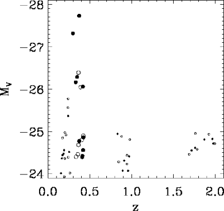
Figure 1: Absolute magnitude versus redshift for quasars observed to date in our HST host-galaxy imaging programmes. Filled circles represent radio-quiet quasars (RQQs) and open circles radio-loud quasars (RLQs). Our earlier work (small symbols) concentrated mainly on quasars of moderate luminosity (typically $M_{V}>-25$) in three redshift regimes ($z\simeq 0.2,1$ & 2), allowing us to probe the evolution of the host galaxies over a large fraction of cosmic history (McLure et al., 1999; Kukula et al., 2001; Dunlop et al., 2003). The current study (large symbols) is designed to explore an orthogonal direction in the $M_{V}-z$ plane, by sampling a large range of quasar luminosities at a single redshift, $z\simeq 0.4$. This is the lowest redshift at which one can find very luminous quasars (those with $M_{V}<-27$), comparable to the most luminous quasars in the high-redshift universe.

Table 2: $V$-band magnitudes and 5 GHz radio flux densities for the quasars in our sample. At the time of writing the majority of the RQQs have only upper limits to their radio fluxes, but these are sufficient to place them safely below the accepted radio-loud/radio-quiet boundary of $L_{5GHz}<10^{-24}$ W Hz^-1 sr^-1. The final column gives the source of the radio data (VCV=Veron-Cetty & Veron (2000); G+99=Goldschmidt et al. (1999); B+96=(Blundell et al.1996). Upper limits from the NVSS were converted to 5 GHz by assuming a radio spectral index $\alpha=0.5$ ($f_{\nu}\propto\nu^{-0.5}$).

Source	Class	$z$	$V$	$S_{5GHz}$	$L_{5GHz}$	Ref.
				(mJy)
Low-luminosity
1237$-$040	RQQ	0.371	16.96	$<0.3$	$<22.14$	G+99
1313$-$014	RQQ	0.406	17.54	$<0.3$	$<22.21$	G+99
1258$-$015	RQQ	0.410	17.53	$<0.2$	$<22.05$	G+99
1357$-$024	RQQ	0.418	17.43	$<0.3$	$<22.24$	G+99
1254$+$021	RQQ	0.421	17.14	$<0.3$	$<22.25$	G+99
1150$+$497	RLQ	0.334	17.10	717.0	25.62	VCV
1233$-$240	RLQ	0.355	17.18	670.0	25.45	VCV
0110$+$297	RLQ	0.363	17.00	340.0	25.17	VCV
0812$+$020	RLQ	0.402	17.10	845.0	25.62	VCV
1058$+$110	RLQ	0.420	17.10	225.0	25.12	VCV
High-luminosity
0624$+$691	RQQ	0.370	14.20	$<1.2$	$<22.75$	NVSS
1821$+$643	RQQ	0.297	14.10	8.6	23.58	B+96
1252$+$020	RQQ	0.345	15.48	0.8	22.50	G+99
1001$+$291	RQQ	0.330	15.50	$<1.2$	$<22.65$	NVSS
1230$+$097	RQQ	0.415	16.15	$<1.2$	$<22.85$	NVSS
0031$-$707	RLQ	0.363	15.50	95.0	24.62	VCV
1208$+$322	RLQ	0.388	16.00	91.0	24.90	VCV

3 Observing strategy

All of our previous HST observations of quasar hosts were carefully designed to maximize the chances of successfully separating the starlight of the host from the PSF of the central quasar. We used the same observing strategy for the current observations and, since some of the quasars in our new sample are significantly more luminous than those in the earlier programmes, these precautions assume even greater importance.

Observing dates for each object are listed in Table 1, along with the name under which the dataset is listed in the HST Archive. The observations were carried out in two different HST observing cycles, although in practice the dates overlap. Observations of the low-luminosity subsample were carried out in Cycle 7 whilst the high-luminosity subsample was observed as part of Cycle 9.

3.1 Choice of filter

As in our previous programmes we selected filters to correspond to $V$-band in the quasar’s restframe. This ensures that our images sample the object’s restframe spectrum longwards of the 4000 Å break, where the starlight from the host is relatively bright, whilst avoiding strong emission lines such as H$\alpha$ and [Oiii]$\lambda 5007$. Despite being directly associated with the quasar activity, ionised emission-line regions can extend over several kiloparsec. By excluding such emission from the images, we obtain a cleaner picture of the distribution of starlight in the hosts.

For the low-luminosity subsample we used the F814W ‘broad $I$’ filter which corresponds closely to the standard Cousins $I$-band. The high-luminosity subsample spans a slightly broader range of redshifts and in order to avoid contamination of the images by emission lines we used the slightly narrower F791W filter.

3.2 Choice of detector

Observations were made with the HST’s Wide Field & Planetary Camera 2 (WFPC2). We opted to use the WF chips ($800\times 800$ pixels, with a scale of 100 mas pixel^-1) since their relatively large pixels offer greater sensitivity to low surface brightness emission. Targets were centred on one of the three WF chips, the exact choice depending on which of the three had performed best over the period immediately prior to the Phase 2 proposal deadline.

3.3 Exposure times

High dynamic range is imperative in a study of this kind in which it is necessary to accurately characterise both the central core of the quasar as well as the faint outer wings of the PSF and the underlying host. The approach used is the same as that tried and tested in our previous works (e.g. McLure et al. 1999, Kukula et al. 2001, Dunlop et al. 2003). We took several exposures of increasing length, with exposure times carefully scaled so that no image would saturate beyond the radius out to which the PSF could be followed in the previous, shorter exposure. The series of exposures were then spliced together in annuli to construct an unsaturated image of the requisite depth (the pointing stability of HST between successive exposures using the FGS fine tracking mode is $\simeq 0.003$ arcsec).

For the ‘low-luminosity’ subsample a single orbit of HST time was sufficient for each object, with exposures of 5, 26 and $3\times 600$ seconds. For the more luminous quasars in the second subsample we required some shorter exposures to avoid saturation of the central pixels, as well as more long exposures to provide greater depth, since the wings of the quasar PSF encroach further out into the surrounding galaxy. Here we devoted two orbits to each object, with exposures of 2, 26, $2\times 100$ and $3\times 600$ seconds in the first orbit and $3\times 700$ seconds in the second.

3.4 PSF determination

Our previous host-galaxy studies have emphasized the importance of characterising the instrumental PSF over a large range in angular radius in order to accurately separate the contributions of host galaxy and active nucleus. The structure of the HST PSF is quite variable, especially at large radii, and depends on its position in the instrument field of view, the SED of the target source and the timing of the observations.

We therefore devoted two orbits of our HST time allocation to obtaining deep, unsaturated stellar PSFs through both the F814W and F791W filters. The star used was GRW$+$70D5824 ($V=12.77$), the same white dwarf used in our previous quasar host-galaxy studies with HST (McLure et al., 1999; Dunlop et al., 2003). This star is an optical standard for WFPC2, and so very accurate photometry is readily available. Its DA3 spectral type and neutral colour ($B-V=0.09$) mimics well the typical quasar SED at the redshift of our sample. In addition, as there are no comparably bright stars within 30 arcsec, we can be sure that our stellar PSF is not contaminated by light from nearby objects. All observations were performed using the same region of the WF chip, within the central 50$\times$50 pixel region.

For the PSF observations we used an observing strategy similar to that for the quasars in order to obtain final images with high dynamic range. A series of exposures were carried out with durations of 0.23, 2.0, 26.0 and 160.0 seconds. Although the increasing exposure times lead to increasing saturation in the core, they never become saturated outside the radius at which the signal-to-noise of the preceding (shorter) exposure has become unsatisfactory. A 2-point dither pattern was also adopted in order to achieve better sampling (the $I$-band PSF is under-sampled by the $0.1$-arcsec pixels of the WF chips). Such a strategy is not employed for the quasar observations, since the read noise introduced by the additional observations results in an unacceptable decrease in signal-to-noise ratio.

4 Data reduction

All the images were passed through the standard WFPC2 pipeline software which performs many of the initial image processing and calibration steps such as dark and bias frame subtraction, along with flat fielding. We carried out three additional reduction steps prior to analysing the images: cosmic-ray decontamination, sky subtraction, and reconstruction of the saturated core regions of both quasar and stellar PSFs by splicing in images with shorter exposures.

4.1 Removal of cosmic rays and bad pixels

Cosmic rays were removed using CRREJ, an iterative sigma-clipping algorithm in iraf, which rejects high pixels from sets of exposures of the same field. The result is a single deep image (with integration time equal to the sum of its parts). This technique however cannot remove the numerous persistent bad or “hot” pixels that appear in the WFPC2 chips. These are listed in a tabular form on the WFPC2 web page and can be incorporated into a mask for modelling purposes (see Section 5).

4.2 Background subtraction

In order to remove a smoothly varying sky background from each image we adopted the following procedure. First, the mean and standard deviation of the background in each image were estimated from a subset of pixels excluding obvious sources. An estimate of the sky distribution was then created by fitting a 2nd order polynomial to each image, having replaced 1$\sigma$ deviations away from the mean background level by the mean value. This smooth sky map was subtracted from each original image to give a final sky-subtracted frame. The background on WFPC2 images is extremely flat, and higher order approximations found to be unnecessary.

4.3 Building deep, unsaturated quasar images

After cosmic ray removal from the deep images, the central regions from the shorter exposures were cut out, multiplied by a factor determined by annular photometry, and substituted into the saturated cores. All steps were performed using standard data-reduction tasks within iraf. For the brightest quasars in our sample, in which the saturated region was large, we spliced together three images in this way to create the final image.

5 Image analysis and modelling

The techniques and software used to perform the 2D modelling have been discussed previously in detail (McLure, Dunlop & Kukula, McLure et al.2000), and in this Section we only briefly reconsider the procedure, highlighting the modifications required to cope with the extreme luminosities of some of the quasars in the current study.

5.1 Quasar models

Each model quasar was constructed by combining a model host galaxy with a central delta function to represent the nuclear point source. We model the host galaxy surface flux using the Sérsic equation (Sérsic, 1968):

$$\Sigma(r)=\Sigma_{0}\exp\left[-\left(\frac{r}{R_{0}}\right)^{\beta}\right]$$ (1)

The surface brightness $\Sigma(r)$ describes an azimuthally-symmetric distribution, which is projected on to a generalised elliptical coordinate system to allow for different eccentricities and orientations of the host galaxy. $R_{0}$ is the characteristic scale length, $\Sigma_{0}$ is the central surface brightness, and $\beta$ describes the overall shape of the profile. We followed the procedure of McLure et al. (1999) and Dunlop et al. (2003) in fitting first to a priori elliptical ($\beta=0.25$) and disc ($\beta=1.0$) models, and then to a more general form in which $\beta$ is a free parameter. Throughout this work we use the term “scale length” to refer to the half-light radius of the host galaxy models; i.e. the radius within which half of the integrated light is contained. For elliptical galaxy models, this half-light radius is equivalent to the often quoted effective radius (or $R_{e}$), while for the disc or spiral models ($\beta=1.0$) the half-light radius and the exponential radius are related by $R_{1/2}=1.68R_{0}$.

Care must be taken in translation from the continuous distribution described by equation 1, to the discrete regime of CCD pixels. Simply basing the surface brightness of each pixel upon the radius of the centre of that pixel is inaccurate, particularly toward the centre, where $\Sigma(r)$ varies non-linearly across the angular width of a pixel. To account for this, galaxy models were calculated at a much higher resolution, and then rebinned to WF chip resolution for comparison with the data. Each pixel value depends upon at least 9 calculations of surface brightness, and up to 676 calculations within the central 0.5 arcsec. Flux is then added to the central pixel of the model galaxy, to represent the unresolved nuclear component.

A given model quasar is thus specified uniquely by a point in the 6-dimensional parameter space $\{\mn@boldsymbol{X}\}=\{L_{N},\Sigma_{0},r_{0},\beta,\Theta,\epsilon\}$:

• $L_{N}=$ luminosity of the nucleus

• $\Sigma_{0}=$ central surface brightness of the host galaxy

• $r_{0}=$ characteristic scale length of the host galaxy

• $\Theta=$ position angle of the host galaxy

• $\epsilon=\frac{a}{b}=$ axial ratio of the host galaxy

• $\beta$ controlling the shape of the profile

The result is an idealised, seeing- and diffraction-free image of a quasar, which can then be convolved with the appropriate PSF to produce a simulated HST observation.

5.2 Modelling the PSF

HST/WFPC2 offers both extremely deep imaging and an extremely well characterised PSF. However, the PSF is under-sampled on the WF chips and care was therefore taken to match the central regions of the PSF to each quasar image. The sub-pixel centring of each quasar image was found using the centroid routine in iraf to characterise the distribution of light in the central region. Accurate oversampled models of the central regions of the PSF were then generated using the tinytim software (Krist, 1999) and were re-sampled using the correct central position to provide an accurate model of the central few pixels of each quasar image.

The tinytim calculation depends upon optical path differences within the Optical Telescope Assembly, and can be performed for any sampling rate, or position within the WFPC2 field-of-view. Using 21-times oversampled (with respect to a WF pixel) PSFs rebinned to the WF chip resolution, we matched the sub-pixel position of the centre of the PSF to each quasar through a 2D minimum $\chi^{2}$ grid search. The best-fit tinytim model was then scaled up (by annular photometry) and spliced into the centre of the deep stellar PSF image. This PSF could then be convolved with the model galaxy plus nuclear component and the result compared to the real quasar image.

5.3 Pixel Error Analysis

The error allocation for such a technique must be done carefully if the $\chi^{2}$ figure of merit is to have real meaning. Inaccurate error weighting may lead to the dominance of one region over another in the fitting, and hence to biased results. Pixel values were assumed to be independent and to obey Poisson statistics. We used a combination of Poisson and sampling errors.

5.3.1 Poisson Noise Error

The minimum possible noise in a given pixel is the combination of Poisson error due to photon shot noise, dark current, and the noise introduced by CCD read-out. However, this simple error calculation severely underestimates the effective error in the central region of our quasar images, due to sub-critical sampling of the steeply rising PSF by the WF pixels.

5.3.2 Sampling Errors

For each quasar image we constructed a “PSF residual” frame by scaling up the PSF to match the quasar in the central pixel and subtracting. The resulting frame can be used to quantify the extent to which the re-sampled tinytim+stellar PSF constructed for that particular quasar image has succeeded in mimicking the central, pixelised flux distribution. Specifically, we compute the inferred remaining sampling error as a function of radius by calculating the variance of the distribution of pixel values in one-pixel wide annuli in this residual image. This variance ($\sigma^{2}$) value is then assigned to each pixel in a given annulus. This is done from the centre out, until the value of this sampling error has fallen (as expected at some radius, given adequate knowledge of the PSF) to the level of the mean Poisson noise error discussed above. We call this radius the “sampling error radius”, $R_{samp}$. We could choose to use this approach across the whole image, since it falls to the same level as the average Poisson noise by a radius of typically $\simeq 1$ arcsec from the centre of the quasar image. However, it is clearly preferable, where possible, to assign each pixel an error based upon its own individual noise properties, rather than a blanket error for an entire annulus. The contribution of genuine galaxy residuals to this error calculation are negligible.

For the two most luminous objects in this study, E1821 and HS0624, the sampling error in the PSF residual image remained above the mean Poisson noise at radii much larger than 1 arcsec. This is because, in these two cases the central quasar is so bright that the image actually contains more information on the detailed structure of the PSF at large radii than does our deepest image of the PSF star. Consequently, for these two objects, the errors in our knowledge of the PSF at radii of several arcsec become important, and we had to enhance the adopted errors in the image at large radii (by typically $\sqrt{2}$; in practice we adopted an average of the ‘sampling’ and Poisson errors at large radius) to achieve an acceptable model fit with a flat distribution of values in the final $\chi^{2}$ image produced by the model-fitting procedure.

5.3.3 Central pixel

No sampling error can be computed for the single central pixel. In this case we apply the Poisson error, noting that the central pixel value has been scaled up from a very short (0.26 seconds) snapshot exposure in order to avoid saturation. The error on the central pixel is typically of the same order as, or a little larger than, the sampling error deduced for the innermost annulus.

5.4 Minimization

The model quasar was convolved with the PSF and, after masking of diffraction spikes and nearby companion objects, compared with the HST data. The $\chi^{2}$ minimum was found for each object within the 6-dimensional parameter space using the downhill simplex method (Press et al., 1992). Six different starting points (spanning the entire parameter space) were used for each object to ensure that the global minimum had been located. This model was checked using three starting simplexes at $\pm$2, 5, and 10% of each best-fitting parameter value. Finally, the model was double-checked by performing a grid search around the best-fit model.

5.5 Photometry

Photometric calibration was performed using the HST headers PHOTFLAM and PHOTZPT, in order to convert counts into physical units of spectroscopic flux density (erg s^-1 cm^-2 Å^-1). In each case, the rest frame filter band is calculated and compared to standard Johnson $V$-band. We assume a simple flat spectrum across the filter bandpass. The internal uncertainty in photometry due to the accuracy of the calibration reference files and the stability of the instrument is 1-2%. The conversion from the HST to the Johnson photometric system also has an uncertainty of a few percent.

6 Results

As described in the previous section, we used two separate modelling strategies in order to determine the morphology of the hosts and the relative contributions of the nuclear and galaxy components. In the first case we fitted a pure de Vaucouleurs ($r^{1/4}$-law) elliptical galaxy and then a pure (exponential) Freeman disc to the host and used the difference in the $\chi^{2}$ values for the two models to decide which model gave the best overall fit. Unless otherwise stated in the notes, all objects were modelled out to a radius of 4 arcsec. Table 3 lists the results of this strategy.

Table 3: Results of model fitting with both de Vaucouleurs spheroid and Freeman disc models. Columns are as follows: object name; best fitting host-galaxy morphology (disc or elliptical); reduced-$\chi^{2}$ value for the best fit model; $\Delta\chi^{2}$ between the chosen and alternative-morphology model; half-light radius, $R_{1/2}$, of best fitting galaxy model in kpc; surface brightness of the host at the half-light radius, $\mu_{1/2}$, in units of $V$ mag.arcsec^-2; integrated absolute magnitudes of the nucleus and the host galaxy, converted from the appropriate filter band (F814W/F791W) to Johnson $V$-band; the ratio of integrated nuclear and host galaxy luminosities; position angle of the host (in degrees, anti-clockwise from vertical in the images); the axial ratio of the host.

IAU name	Morphology	$\chi^{2}_{red}$	$\Delta\chi^{2}$	$R_{1/2}$	$\mu_{1/2}$	$M_{V}^{nuc}$	$M_{V}^{host}$	$L_{N}/L_{H}$	PA	$a/b$
	(best fit)			(kpc)					(∘)
Radio-Quiet Quasars
0624$+$691	Elliptical	$1.488$	$486.2$	$9.7\pm 0.7$	$22.0\pm 0.15$	$-27.18$	$-24.01$	18.45	140	1.2
1001$+$291	Elliptical	$1.318$	$326.3$	$15.4\pm 0.6$	$23.1\pm 0.10$	$-25.62$	$-23.47$	7.27	58	1.7
1230$+$097	Elliptical	$1.219$	$107.7$	$5.8\pm 0.2$	$21.7\pm 0.13$	$-25.24$	$-23.24$	6.26	1	1.3
1237$-$040	Disc	$1.323$	$334.5$	$6.7\pm 0.1$	$22.0\pm 0.05$	$-23.98$	$-22.63$	3.46	14	1.1
1252$+$020	Elliptical	$1.228$	$102.0$	$3.9\pm 0.5$	$22.1\pm 0.30$	$-25.26$	$-22.04$	19.47	150	1.1
1254$+$021	Elliptical	$1.356$	$646.3$	$14.2\pm 0.3$	$23.2\pm 0.05$	$-23.91$	$-24.00$	0.92	30	1.1
1258$-$015	Elliptical	$1.352$	$14.4$	$1.5\pm 0.2$	$19.8\pm 0.25$	$-23.77$	$-22.33$	3.77	140	1.1
1313$-$014	Disc	$1.254$	$351.0$	$5.6\pm 0.1$	$21.7\pm 0.06$	$-23.74$	$-22.68$	2.65	174	1.1
1357$-$024	Disc	$1.257$	$457.1$	$5.8\pm 0.1$	$21.9\pm 0.05$	$-23.66$	$-22.47$	2.99	160	1.2
1821$+$643	Elliptical	$1.828$	$570.4$	$18.9\pm 0.2$	$22.9\pm 0.05$	$-27.14$	$-24.33$	13.35	113	1.3
Radio-Loud Quasars
0031$-$707	Elliptical	$1.268$	$802.8$	$11.0\pm 0.4$	$23.1\pm 0.08$	$-23.84$	$-23.21$	1.80	70	1.2
0110$+$297	Elliptical	$1.327$	$561.1$	$12.3\pm 0.8$	$23.6\pm 0.12$	$-23.93$	$-22.99$	2.39	31	1.2
0812$+$020	Elliptical	$1.509$	$904.7$	$17.4\pm 0.3$	$23.6\pm 0.05$	$-24.80$	$-23.81$	2.49	155	1.2
1058$+$110	Elliptical	$1.390$	$135.5$	$13.1\pm 1.1$	$24.1\pm 0.14$	$-23.58$	$-22.69$	2.28	159	1.3
1150$+$497	Elliptical	$1.360$	$340.6$	$8.3\pm 0.3$	$22.1\pm 0.11$	$-24.09$	$-23.28$	2.11	174	1.5
1208$+$322	Elliptical	$1.096$	$49.1$	$6.5\pm 0.1$	$22.2\pm 0.05$	$-25.01$	$-22.50$	10.06	7	1.9
1233$-$240	Elliptical	$1.358$	$47.7$	$3.1\pm 0.1$	$20.6\pm 0.05$	$-24.78$	$-22.98$	5.23	58	1.1

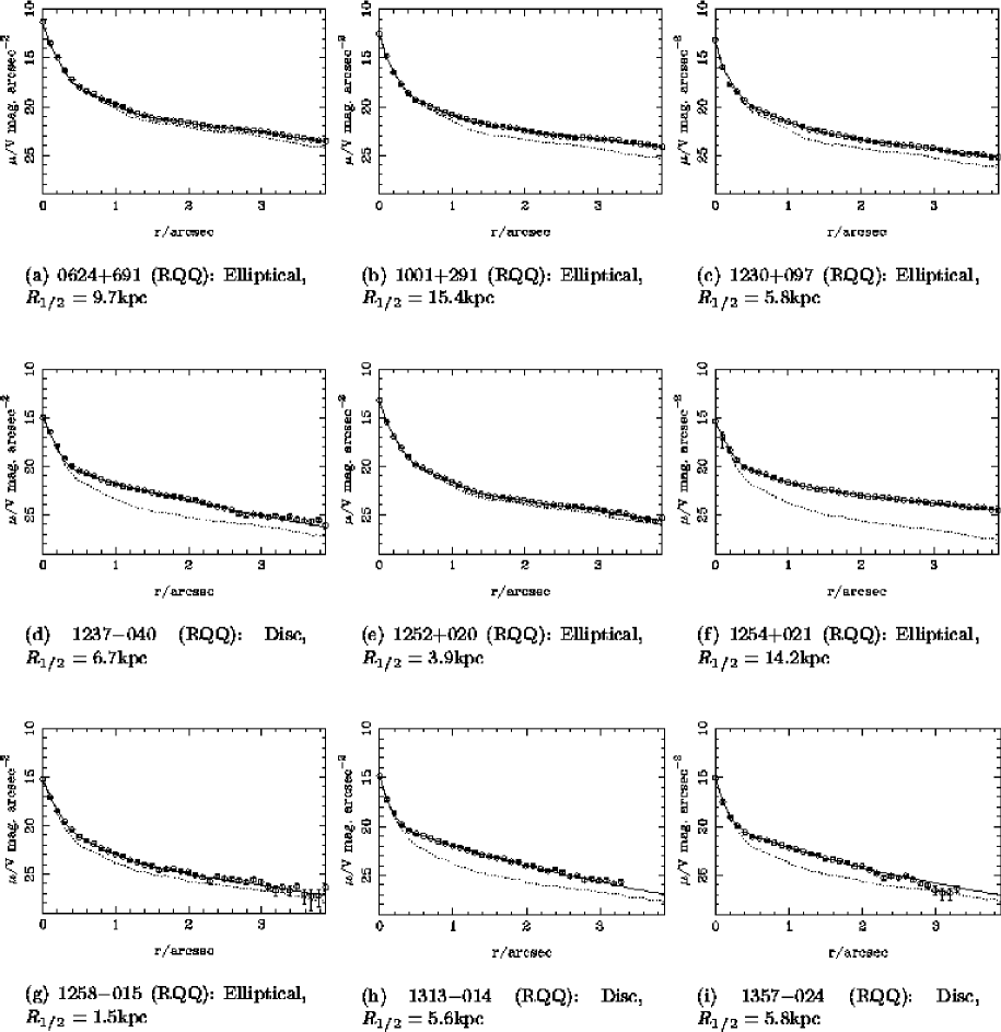
Figure 2: The radial profiles of the best-fitting bulge or disc models for the 17 quasars in our sample. Each plot shows the azimuthally averaged image data (open circles with $1\sigma$ error bars), the azimuthally averaged best-fit model after convolution with the PSF (solid line) and the azimuthally averaged best-fit unresolved nuclear component after convolution with the PSF (dotted line). The form of the fit (disc or elliptical) and the scale length ($R_{1/2}$) of the model galaxy are also given beneath each panel.

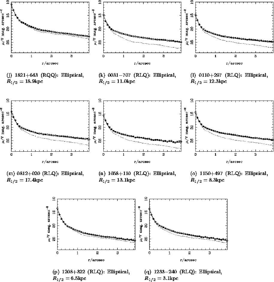
Figure 2: - continued

In the second case, we carried out modelling using a variable-$\beta$ fit, in which the $\beta$ parameter of equation 1 is allowed to vary freely. This allows for a more general morphology than the strictly disc or bulge technique. Table 4 shows the results of this variable-$\beta$ fitting which, for the most part, rather impressively reinforces the results of the fixed-$\beta$ models. However there are a few objects in which the variable-$\beta$ technique returned a hybrid value and these are noted in the entry for the relevant object in the Appendix.

Greyscale images of the individual objects are also presented in the Appendix. For each quasar we show the final reduced $I$-band (F814W/F791W) HST image (top left), the best-fitting model quasar (nuclear point source plus either pure bulge or pure disc host galaxy) to the quasar image (top right), the model host galaxy only (bottom left) and the model-subtracted residual image (bottom right). Radial profiles for the best-fit bulge and disc models are presented in Fig.2.

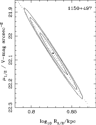
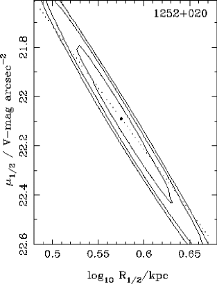
Figure 3: $\chi^{2}$ contours (at $1-3\sigma$ levels) in the $\mu-R$ plane for 1150$+$497 (left), and 1252$+$020 (right). In each case, the best-fit solution is marked by a dot. The figure demonstrates the degeneracy that remains between galaxy size and surface brightness, even when any confusion between host and nuclear light has been eliminated. 1150$+$497 is a typical example of the objects in this study and the contours describe a slope close to 5 (dashed line), as expected if the host galaxy’s luminosity has been correctly constrained. Of all the objects in our sample, 1252$+$020 has the least robust host luminosity constraint, the contours lying along a somewhat steeper slope of $\simeq 5.7$. One other object, 1258$-$015, exhibits slightly steep contours, having a slope of $\simeq 5.6$. In these latter 2 cases there is clearly still some degeneracy between host and nuclear flux.

We can gain further insight into how successful we have been in disentangling the host galaxy from the nucleus through investigation of the $\chi^{2}$ contours in the $\mu_{1/2}-R_{1/2}$ plane (e.g. Fig.3). For any quasar in which we have successfully characterised the host luminosity (i.e. eliminated the degeneracy between host and nuclear contributions), these contours should lie along a slope of 5.0 (see e.g. Abraham, Crawford & McHardy Abraham, Crawford & McHardy1992; Malkan 1984), and allow us to assess how well constrained these two parameters are.

Table 4: Outcome of variable-$\beta$ modelling. Columns are as follows: object name; best-fit morphology from pure bulge & disc models (Table 3); best-fit $\beta$ value with no assumed morphology; the value of reduced-$\chi^{2}$ produced by this best-fit model; improvement in fit, $\Delta\chi^{2}$ obtained by using the variable-$\beta$ technique compared to the best-fit fixed morphology model.

IAU name	Morph.	$\beta$	$\chi^{2}_{red}$	$\Delta\chi^{2}$
Radio-Quiet Quasars
0624$+$691	Elliptical	0.20	1.485	42.2
1001$+$291	Elliptical	0.26	1.318	0.1
1230$+$097	Elliptical	0.37	1.216	12.0
1237$-$040	Disc	0.96	1.321	0.6
1252$+$020	Elliptical	0.22	1.227	0.7
1254$+$021	Elliptical	0.24	1.356	2.0
1258$-$015	Elliptical	0.26	1.351	2.0
1313$-$014	Disc	0.97	1.254	0.2
1357$-$024	Disc	1.32	1.246	22.8
1821$+$643	Elliptical	0.22	1.771	485.4
Radio-Loud Quasars
0031$-$707	Elliptical	0.26	1.266	11.9
0110$+$297	Elliptical	0.22	1.323	15.5
0812$+$020	Elliptical	0.23	1.503	9.5
1058$+$110	Elliptical	0.33	1.388	6.9
1150$+$497	Elliptical	0.36	1.356	19.4
1208$+$322	Elliptical	0.32	1.091	19.5
1233$-$240	Intermediate	0.56	1.361	57.2

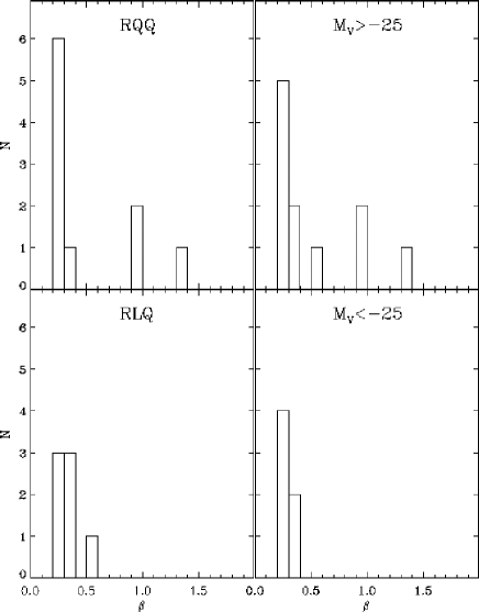
Figure 4: Histograms of the best-fit $\beta$ values from our variable-$\beta$ models. $\beta=0.25$ is equivalent to an $r^{1/4}$ de Vaucouleurs law, $\beta=1$ is an exponential Freeman disc. In the panel to the left we divide the sample in terms of radio luminosity. On the right, the sample is divided according to optical absolute magnitude. Clearly all optically-luminous, and all radio-loud objects lie in bulge-dominated hosts, confirming and extending the trends deduced by Dunlop et al. (2003).

7 Discussion

The quasars imaged in this study span almost two orders of magnitude in optical luminosity but only a narrow range of redshifts. They therefore allow us to investigate the relationship between galaxies and their central black-holes, and the relative roles of black-hole mass and fuelling efficiency in determining quasar luminosities.

We have successfully recovered a host galaxy for each one of the 17-strong sample. In general, the host size and central surface brightness have been constrained to within a few kiloparsecs, and half a magnitude, respectively, as is illustrated by the typical joint confidence region illustrated in the left-hand panel of Fig.3. However, there are two objects, the RQQ’s 1252$+$020, and 1258$-$015 for which the fit yields poor stability for the host properties, and the resulting much larger confidence region for 1252$+$020 is shown in the right-hand panel of Fig.3. Overall host and nuclear fluxes are typically constrained to better than 0.1mag by the modelling software, with a similar uncertainty due to the conversion from ST mags to standard $V$-band.

7.1 Host galaxy morphologies

With regard to basic host galaxy morphology, the results of this study are quite clear cut, and confirm and extend the findings of Dunlop et al. (2003). For every quasar host the modelling software yielded a clear decision in favour of either a disc-dominated or bulge-dominated host. Moreover, in virtually every case this preference was confirmed by the variable-$\beta$ model, which returned a value of $\beta$ very close to either $0.25$ (elliptical) or $1$ (disc).

At this point it is important to clarify what we mean by “bulge-dominated” or “disc-dominated” galaxies. Our modelling software finds the best overall fit to the light from the quasar and its host galaxy. This is dominated by contributions from the point-like nucleus itself, and from the smooth, high SNR host region far from the nucleus. Our HST images are of sufficient depth that we expect to be able to detect large features at least as dim as $V=27$ mag.arcsec^-2. To place this in some context, this is a sufficient depth that the prominent tidal arm in Mrk1014, could be easily be detected if it were placed at a $z\sim 1$. However, close to the nucleus, this sensitivity is impaired by our lack of knowledge of the form of the PSF, and here a small-scale, relatively bright feature might go unnoticed by the model. Such features can be exposed in our residual images, which show the best fit model subtracted from the data. Thus when we claim to detect bulge or disc-dominated hosts, we mean just that: on large scales of a few kpc, the host light is dominated by smooth emission that follows a spheroidal ($r^{1/4}$-law) or a disc-like (exponential) profile. There obviously remains the possibility of a small, centrally concentrated bulge component in the disc-dominated hosts, and in an effort to address this, we attempted a 2-component modelling technique. This is simply an extension of the modelling technique described above, with individual disc and bulge components each described in full by 4 parameters, giving a 9-dimensional model overall. The results are presented in table 5: A significant spheroidal component is found in two of the three disc-dominated hosts; 1237$-$040 and 1313$-$014.

Table 5: Results of the 2-component model fitting to the disc-dominated hosts. The improvement in the fit over the simple disc case is given in column 3. The nuclear luminosity, and the scale-length and luminosity of each host galaxy component are given in columns 4-8, with the bulge: disc ratio in the final column.

Source	Morph.	$\Delta\chi^{2}$	$M_{V}(\mathrm{Nuc})$	$r_{B}$	$M_{V}(\mathrm{Bulge})$	$r_{D}$	$M_{V}(\mathrm{Disc})$	Bulge/Disc
				kpc		kpc
1237$-$040	D/B	10.8	$-23.96$	3.8	$-21.18$	6.5	$-22.46$	0.31
1313$-$014	D/B	4.7	$-23.72$	3.3	$-20.28$	5.6	$-22.62$	0.12
1357$-$024	D	0.3	$-23.65$	0.4	$-18.38$	6.3	$-22.47$	0.023

As illustrated in Fig.4, the three quasars in the current sample for which we find disc-dominated hosts are, i) radio-quiet, and ii) in the low-luminosity sub-sample with $M_{V}>-25$. In fact, reference to Table 3 reveals that the three disc-dominated hosts house nuclei with $M_{V}>-24$. Furthermore, the brightest of the three quasars (1237$-$040), is found to have a significant spheroid. This result therefore meshes well with the luminosity-dependence of host-galaxy morphology illustrated in Fig.10 of Dunlop et al. (2003); disc-dominated host galaxies are not found for nuclei with $M_{V}<-24$. In one other case (1313$-$014) we detect a spheroidal component at low luminosity ($M_{V}=-20.28$), suggesting an accretion rate around $L/L_{Edd}\simeq 3$, assuming the local $M_{BH}-M_{\mathrm{S}ph}$ ratio McLure & Dunlop (2002). In the final disc-dominated object (1357$-$024) we detect no significant bulge component. However, for a roughly Eddington-limited accretion rate, we would anticipate a bulge luminosity of around $M_{V}=-20.8$. Such a bulge is expected to have a scalelength of $\simeq 3$kpc, and could be difficult to distinguish from the unresolved nuclear light.

As discussed by Dunlop et al. (2003), this result can now be viewed as a natural consequence of the now well-established proportionality of black-hole and spheroid mass.

7.2 Host galaxy scale lengths and luminosities

Table 3 lists the scale lengths and luminosities for the best-fit fixed-morphology models. Once again, the results are broadly consistent with those of McLure et al. (1999) and Dunlop et al. (2003); the hosts are generally large, luminous galaxies.

Three of the five smallest galaxies are the disc-dominated hosts. There is a tendency for the hosts of the RLQs to be slightly larger than those of the RQQs, but this is not statistically significant.

$$\langle R_{1/2}\rangle_{(RLQ)}=10.2\pm 1.8\mathrm{kpc}$$

$$\langle R_{1/2}\rangle_{(RQQ)}=8.7\pm 1.8\mathrm{kpc}$$

On average the more luminous quasars also have slightly larger hosts, but again the mean values for the two subsamples are in agreement given the statistical uncertainty.

$$\langle R_{1/2}\rangle_{(M_{N}<-25)}=10.0\pm 2.4\mathrm{kpc}$$

$$\langle R_{1/2}\rangle_{(M_{N}>-25)}=9.0\pm 1.5\mathrm{kpc}$$

We find that that all the hosts are more luminous than $L^{\star}$ ($M_{V}^{\star}=-21.0$; Efstathiou, Ellis & Peterson 1988). There is no statistically significant difference between the average values for each subsample, but these basic statistics should not obscure the fact that the two quasars in the sample with $M_{V}(Nuc)<-27$ are also the only two objects for which we find $M_{V}(Host)<-24$.

$$\langle M_{V}(Host)\rangle_{(RLQ)}=-23.06\pm 0.16$$

$$\langle M_{V}(Host)\rangle_{(RQQ)}=-23.12\pm 0.25$$

$$\langle M_{V}(Host)\rangle_{(M_{N}<-25)}=-23.27\pm 0.36$$

$$\langle M_{V}(Host)\rangle_{(M_{N}>-25)}=-23.01\pm 0.16$$

7.3 Kormendy relation

The Kormendy relation is the photometric projection of the fundamental plane exhibited by elliptical galaxies. The host galaxies of the quasars in our sample follow a Kormendy relation of the form

$$\mu_{1/2}=(19.2\pm 0.6)+(3.33\pm 0.7)log_{10}R_{1/2}$$ (2)

shown in Fig.5 (where we have plotted and fitted only those with bulge-dominated hosts). A galaxy with a well-constrained luminosity but unknown scale length will lie along a locus with a slope of 5, illustrated by the error ellipse in the top right corner of this figure (c.f. Fig.3). The slope of 3.33 is in excellent agreement with that determined recently for 9000 early-type galaxies ($3.33\pm 0.09$) drawn from the SDSS by (Bernardi et al.2003) and is sufficiently different to a slope of 5 to convince us that the surface brightnesses and scale lengths of the hosts have been well constrained.

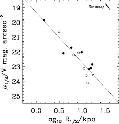
Figure 5: The scale length ($R_{1/2}$) vs surface brightness ($\mu_{1/2}$) projection of the fundamental plane. Filled circles represent RQQ hosts, open circles RLQ hosts (bulge-dominated hosts only). The solid line shows the best fit Kormendy relation to the sample and has the form $\mu_{1/2}=(19.2\pm 0.6)+(3.33\pm 0.7)log_{10}R_{1/2}$. The narrow ellipse in the top right corner of the plot shows the $2\sigma$ error contours for 1258$-$015; its slope of 5 is due to the remaining degeneracy between size and surface brightness when host luminosity has been well constrained.

7.4 The role of galaxy mergers and interactions

Interactions and merging events between galaxies have long been suggested as the triggering events for the activation of quasars, especially at low redshifts where some mechanism is required to initiate fuelling of the black-holes in otherwise stable, gas-depleted ellipticals. Indeed, most host galaxy studies to date have found that indications of disturbance such as tidal tails, multiple nuclei and close companions are present in around 50% of quasar hosts (e.g. Smith et al. 1986; Hutchings & Neff 1992; Bahcall et al.1997). However Dunlop et al. (2003) point out that this is also true of inactive massive ellipticals, so that it is not clear whether mergers are genuinely a defining feature of quasar hosts or merely the legacy of their parent population. Certainly many quasar hosts appear to be entirely undisturbed, so clearly a large-scale disruption of the host is not always necessary to trigger fuelling of the central engine (or at least the timescales for relaxation after the merger event and of fuel reaching the central engine may sometimes be vastly different).

The residual images of the quasars in the current study (see Appendix), provide a means of identifying signs of galaxy interactions which might not be obvious in the raw HST images. They are produced by subtracting the best-fitting axially-symmetric quasar model from the HST image. Since the model only attempts to fit the smooth underlying distribution of galaxy light, any additional structures (spiral arms, bars, tidal tails, double nuclei etc) will be made more obvious in the residual image.

In our sample we find unambiguous evidence for an ongoing galaxy interaction in only one object, the RQQ 1237$-$040. Several other objects are candidates for some form of disturbance having taken place (for instance the RQQ 1001$+$291 with its prominent spiral arms and large-scale de Vaucouleurs profile), or have other objects within a few arcsec on the sky which might conceivably be interacting if they lie at the same redshift. In fact the majority of our quasars appear to have some companions nearby on the sky, which is at least suggestive of a cluster environment.

However we find no correlation between the luminosity of the quasar and the presence of any morphological disturbance in the host. In our small sample, at least, the most luminous quasars seem no more likely to be interacting systems than their less luminous counterparts.

7.5 Black-hole masses

Reliable black-hole masses are available for at least 37 nearby galaxies (Kormendy & Gebhardt, 2001), highlighting the correlations which exist between spheroid luminosity and black-hole mass (e.g. Magorrian et al.1998), and between spheroid velocity-dispersion and black-hole mass (, Gebhardt et al.2000; Ferrarese & Merritt, 2000). As discussed by McLure & Dunlop (2002), both these relations for inactive ellipticals, and the results of H$\beta$-derived virial black-hole estimates in active objects, are consistent with a direct proportionality of black-hole and spheroid mass of the form $M_{BH}=0.0012M_{\mathrm{S}ph}$, with a typical scatter of 0.3 dex.

We used the luminosities from our best-fit bulge-dominated galaxy models to estimate host-galaxy masses, given an estimate of the mass-to light ratio of an early-type galaxy (Jørgensen, Franx & Kjaergaard, 1996); $(M/L)_{R-band}\propto L^{1.31}$. We then used the black-hole:spheroid mass relation above to estimate black-hole masses for the quasars, independent of their observed nuclear output. The results of this calculation are given in column 3 of Table 6. Once again, this has only been performed for the bulge-dominated hosts. A similar calculation can be performed for the spheroidal components of the disc-dominated hosts (see end of section 7.1). The median black-hole masses for the high and low-luminosity subsamples are:

$$\langle M_{BH})_{(M_{N}<-25\rangle}=(1.1\pm 1.0)\times 10^{9}$$

$$\langle M_{BH})_{(M_{N}>-25\rangle}=(0.5\pm 0.3)\times 10^{9}$$

We find that all of the host galaxies are sufficiently massive ($M_{\mathrm{S}ph}>10^{11}M_{\odot}$) to contain a black-hole in excess of $10^{8}M_{\odot}$, but the difference in mass between the black-holes in optically powerful and optically weak quasars is not large enough to account for the factor $\sim 10$ increase in luminosity. Unfortunately, no direct measures of black-hole mass are available for any of the objects in our sample. A comparison with, for example, a Virially estimated black-hole mass would provide an extremely valuable test.

7.6 Fuelling efficiencies

We can now calculate the predicted luminosity of each bulge-dominated object if the black-hole were to radiate at its Eddington limit ($L_{Edd}^{Bol}=1.26\times 10^{31}\frac{M_{BH}}{M_{\odot}}$ Watts) and compare this with the actual luminosity of the quasar nucleus obtained from our model fitting. The results of this procedure are listed in columns 4 and 5 of Table 6, and plotted in Fig.6; there is clearly no correlation between black-hole mass and fuelling efficiency. However, one can immediately see a clearer distinction between our luminous and dim subsamples than was apparent simply from their estimated black-hole masses:

$$\langle\frac{L_{N}}{L_{Edd}}\rangle_{(M_{N}<-25)}=0.78\pm 0.2$$

$$\langle\frac{L_{N}}{L_{Edd}}\rangle_{(M_{N}>-25)}=0.17\pm 0.03$$

If we exclude the relatively poorly constrained luminous RQQ 1252$+$020 (which appears, from our modelling, to exceed the Eddington limit), the median Eddington ratio for the luminous subsample drops to 0.47, but this is clearly still significantly higher than for the low-luminosity sample.

Object	Morph.	$M_{\mathrm{S}ph}$	$M_{BH}$	$M_{V}^{Edd}$	$\frac{L_{N}}{L_{Edd}}$
		($10^{11}M_{\odot}$)	($10^{9}M_{\odot}$)
Radio-Quiet Quasars
0624$+$691	E	13.90	1.67	$-27.28$	0.91
1001$+$291	E	7.27	0.87	$-26.57$	0.42
1230$+$097	E	5.51	0.66	$-26.27$	0.39
1252$+$020	E	1.29	0.16	$-24.70$	1.67
1254$+$021	E	13.70	1.65	$-27.27$	0.05
1258$-$015	E	1.84	0.22	$-25.08$	0.30
1821$+$643	E	20.50	2.46	$-27.70$	0.60
Radio-Loud Quasars
0031$-$707	E	5.31	0.64	$-26.23$	0.11
0110$+$297	E	4.07	0.48	$-25.94$	0.16
0812$+$020	E	11.00	1.31	$-27.02$	0.13
1058$+$110	E	2.84	0.34	$-25.55$	0.16
1150$+$497	E	5.78	0.69	$-26.32$	0.13
1208$+$322	E	2.26	0.27	$-25.30$	0.76
1233$-$240	E	4.02	0.48	$-25.93$	0.35

Table 6: Galaxy spheroid and black-hole mass estimates for each of the bulge-dominated quasars in our sample. The table also lists the theoretical Eddington luminosity, $M_{V}^{Edd}$, of each black-hole, and the efficiency at which the black-hole is accreting expressed as the ratio of the luminosity ascribed by our model to the nuclear point source to the Eddington luminosity predicted by the model of the host galaxy ($L_{N}/L_{Edd}$). Note that the RQQ 1252$+$020 appears to be accreting at a super-Eddington rate. This object has the least robust model fit of the entire sample, and it is likely that the nuclear flux has been overestimated. Results for the spheroidal components of the three disc-dominated objects are presented where detected. Both detections (1237$-$040 and 1313$-$014) yield slightly super-Eddington accretion rates, whilst the nuclear luminosity of 1357$-$024 can be explained in terms of Eddington-limited accretion in an undetected, compact central bulge at $M_{V}\simeq-20.8$.

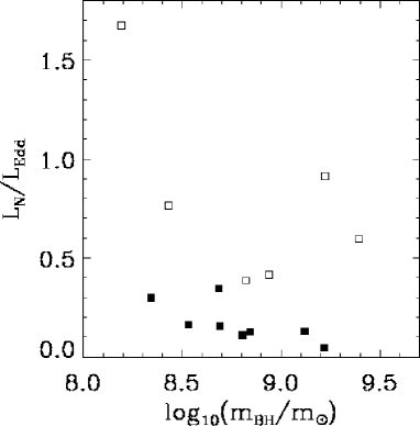
Figure 6: Quasar efficiency as a function of the Eddington luminosity versus black-hole mass, as determined from the spheroid luminosity. Only bulge-dominated objects are plotted, and they have been divided into optically luminous (open squares) and optically dim (solid squares) subsamples at $M_{V}(Nuc)=-25$, as discussed in the text. Our model fit to the RQQ 1252$+$020 implies that the object has a small host with an extremely luminous nucleus, yielding a super-Eddington luminosity. However, the quality of the model fit is poor, and this value is quite likely erroneous. Overall there is no obvious tendency for fuelling efficiency to vary as a function of black-hole mass, and the increase in luminosity across the sample reflects an increase both in black-hole mass, and accretion efficiency.

Thus, within our $z=0.4$ sample, increasing quasar luminosity appears, on average, to reflect a mix of both larger black-hole mass, and increased fuelling efficiency. Not surprisingly, the only two quasars in the present sample with $M_{V}<-27$ have the two most massive black-holes.

A number of other features of the results summarised in Table 6 are worthy of comment. First, while inferred fuelling efficiencies range over an order of magnitude, we find no evidence for super-Eddington accretion. If one excludes the poorly constrained RQQ 1252$+$020, the most efficient emitter is 0624$+$691, with $L_{N}/L_{Edd}\simeq 1$. Second, the most massive central black-hole found in our sample has a mass of $3\times 10^{9}{\rm M_{\odot}}$, comparable to the inferred mass of the super-massive black-holes at the centres of M87 (Marconi et al., 1997) and Cygnus A (Tadhunter et al., 2003). Thus, the basic physical quantities derived for the quasars in our sample appear to be entirely reasonable, requiring neither unorthodox methods of accretion, nor surprisingly massive black-holes.

It is important to note that the black-hole mass calculation applied above (and hence the values of $M_{BH}$ and $L_{N}/L_{Edd}$ given in table 6 and Fig.6) assume a single, fixed value for the black-hole:spheroid mass ratio. At some level, this is clearly unrealistic and it is therefore not in fact obvious to what extent the scatter in the nuclear:host ratio reflects a range of fuelling efficiency. Accordingly, we conclude this paper with the first exploration of the extent to which scatter in nuclear:host ratio can or cannot be explained by intrinsic scatter in the underlying black-hole:spheroid mass relationship.

7.7 Black-hole mass versus fuelling rate

The nature of the link between quasar luminosity and black-hole mass is more easily explored by plotting host versus nuclear luminosity. This is shown in Fig.7 where we have plotted the absolute magnitudes of the hosts against those of the nuclei in our sample (circles), with $100\%$, $10\%$ and $1\%$ of the Eddington limit shown as solid, dashed and dotted lines respectively. Shown also are points from Dunlop et al. (2003) (diamonds) and McLeod, Rieke & Storrie-Lombardi (1999) (triangles), converted to rest-frame $V$-band, and our adopted cosmology. We have also included 3 objects from the sample of Percival et al. (2001) (stars), for which archival HST images are now available (0043$+$039, 0316$-$346 and 1216$+$069). It now seems likely that seeing limitations in this ground-based study effectively prevented successful disentanglement of host and nuclear fluxes, and accurate morphological distinctions. The replacement images from the HST archive have been analysed in precisely the same way as has been described for the present sample, and converted into rest-frame $V$-band.

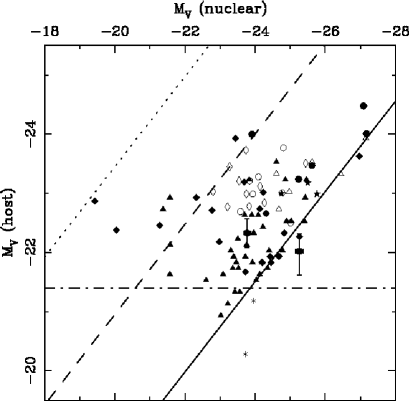
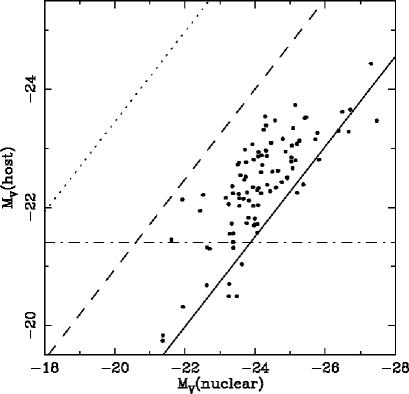
Figure 7: Upper panel: Host versus nuclear luminosity for the bulge-dominated quasars in the current sample (circles). The spheroidal components of the two disc-dominated quasars, 1258$-$015 and 1237$-$040 are shown by asterisks. The samples of McLeod et al. (1999) (triangles), and Dunlop et al. (2003) (diamonds), plus three objects from Percival et al. (2001) re-imaged with the HST (stars - see main text) are also presented. Filled symbols once again denote radio-quiet objects, and open symbols radio-loud objects. The solid, dashed and dotted lines represent objects radiating at 100%, 10% and 1% of the Eddington luminosity respectively on the assumption of a fixed black-hole to bulge mass ratio of $M_{BH}=0.0012M_{\mathrm{S}ph}$. The majority of the quasars in our sample appear to be radiating at $>$10% of their Eddington limit (the single super-Eddington object is the poorly constrained 1252$+$020 - see Fig.3.). Error bars are smaller than the symbols for all objects except for 1252$+$020 and 1258$-$015. Lower panel: The predicted distribution on the host versus nuclear luminosity plane for a sample of quasars radiating at 50% of the Eddington limit, given an adopted scatter of 0.3 dex in the black-hole:spheroid mass relation, and including the effect of the exponential cutoff in the luminosity function above $L^{\star}$ (dot-dashed line). The random sample has been resampled in order to reflect the the same distribution of nuclear luminosities as is displayed by the combined data in the upper panel. This scenario re-produces much (but not all of) the observed scatter in apparent fuelling efficiency without in fact requiring a range of Eddington ratios. However, at the same time an assumed scatter of 0.3 dex or lower is required to avoid too many objects apparently breaching the rather solid Eddington limit displayed by the data.

The top panel of Fig.7 shows that, while central black-holes appear to accrete with a wide range of efficiencies, the objects we term quasars are generally produced by black-holes emitting at $>10$% of their Eddington limit, residing in host galaxies with $L>L^{\star}$. However, perhaps the most impressive feature of this plot is that, for a given host galaxy luminosity, the most luminous nuclear source has a luminosity essentially exactly as would be predicted from the Eddington limit corresponding to the mass of the central black-hole as deduced from the relationship $M_{BH}=0.0012M_{\mathrm{S}ph}$. In other words, while the statistical correlation between host-galaxy and nuclear luminosity within these samples may not be very strong, the relationship between host-galaxy and maximum nuclear luminosity appears extremely tight, and completely consistent with Eddington limited accretion. Such a result has previously been noted by McLeod & Rieke (1995) for lower-luminosity AGN, but to the best of our knowledge, this is the first time that it has been demonstrated concretely at high luminosity. So clean is this relation over two orders of magnitude in $L_{N}$ that it has the potential to constrain the size of the scatter in the underlying black-hole:spheroid relation for massive galaxies. In turn, such constraints can then illuminate the extent to which the apparent $~{}1$ dex scatter in fuelling efficiency can also be explained by intrinsic scatter in the underlying black-hole:spheroid mass relationship.

A full exploration of this approach is beyond the scope of the present paper and is in any case better applied to larger and more statistically complete samples. However, we have produced the lower panel of Fig.7 to illustrate the extent to which the data can be reproduced by folding in an assumed underlying scatter in the black-hole:spheroid mass ratio, while assuming a single value for the Eddington ratio.

We generated a random population of spheroidal galaxies, and central black-holes defined by a Schechter function with $\alpha=1.25$ and $log_{10}(\frac{M_{tot}^{*}}{M_{\odot}})=11.5$ (where $M_{tot}^{*}$ denotes the turnover in the distribution of total mass, stellar and dark matter), and assuming a fixed scatter in the black-hole:spheroid mass relation. From this galaxy / black-hole population we generate a sample of quasars, assuming a fixed fuelling efficiency, and constrained to share the same nuclear luminosity distribution as is found for the real sample in the top panel of Fig.7.

Adoption of a scatter larger than 0.3 dex produces significantly more apparently super-Eddington objects than are observed. Conversely, adoption of a scatter substantially smaller than 0.3 dex can reproduce the apparently tight Eddington limit more closely, but underpredicts the apparent scatter in fuelling efficiency, and cannot therefore reproduce the tight Eddington limit displayed by the data in the top panel of Fig.7.

We used a 2D K-S test to compare the simulation with the data. By marginalising over universal efficiency we find the probability, $p$, that the quasar sample is consistent with a fixed fuelling efficiency. We find that for a 0.3dex or smaller scatter, the quasar sample is inconsistent with a population in which there is a fixed fuelling efficiency ($p=0.022$). Increasing the scatter produces an improvement to acceptable levels at 0.4dex ($p=0.157$) and 0.45dex($p=0.198$), but a scatter as large as 0.5dex is strongly excluded ($p=0.002$).

The figure presented illustrates the situation for a sample of quasars radiating at 50% of the Eddington limit, with an assumed scatter in the underlying black-hole:spheroid mass relation of 0.3 dex. These values were chosen for this illustration as the combination which best reproduces both the apparently tight Eddington limit, and level of scatter displayed by the data in the upper panel of Fig.7, adequately describing the spread in nuclear luminosities at $M_{V}<-23$. However, for dimmer quasars, we find that a variable fuelling rate is essential in order to explain the full range in $\frac{L_{N}}{L_{H}}$ observed.

In summary, from simulations of the sort described above, the observed apparent tight upper (Eddington) limit on fuelling efficiency can be used to set an upper limit of 0.3 dex on the scatter in the underlying black-hole:spheroid mass relation, consistent with other recently derived values (McLure & Dunlop, 2002; Marconi & Hunt, 2003). A significant fraction of the scatter observed in the upper panel of Fig.7 can then still be attributed to the scatter in the underlying mass relationship, but some variation in assumed efficiency would still seem to be required to reproduce the most underluminous objects.

Finally, we can use the tightness of the bound placed by the Eddington line to place constraints on the hosts of higher redshift quasars, where direct imaging of the host is not possible. A quick inspection of Fig.7 reveals that any quasar brighter than $M_{V}=-27$ must be found in, or at least end up within, a spheroidal galaxy brighter than $M_{V}=-24$, and must be radiating at a rate close to its Eddington limit. The turnover in the Schechter function places a natural limit on the abundance of such large galaxies, and the data appear to show just such a cutoff at a host luminosity of $M_{V}\simeq-24.5$.

8 Summary

Through the careful analysis of deep HST images, we have succeeded in determining the basic properties of the host galaxies of quasars spanning a factor of $\simeq 20$ in luminosity, but within a narrow redshift range at $z\simeq 0.4$. The sample under study contains both radio-loud and radio-quiet quasars, and includes some of the most luminous quasars known in the low-redshift universe.

Our results confirm and extend the trends uncovered in our previous HST-based studies of lower luminosity objects (McLure et al., 1999; Dunlop et al., 2003). Specifically we find that the hosts of all the radio-loud quasars, and all the radio-quiet quasars with $M_{V}<-24$ are giant elliptical galaxies, with luminosities $L>L^{\star}$, and scale lengths $R_{e}\simeq 10$ kpc. Moreover, the Kormendy relation displayed by these host galaxies is indistinguishable from that displayed by nearby, inactive ellipticals.

From the luminosities of their hosts we have estimated the masses of the black-holes which power the quasars using the relationship $M_{BH}=0.0012M_{\mathrm{S}ph}$ and hence, via comparison with the quasar nuclear luminosities, also the efficiency with which each black-hole is emitting relative to the Eddington limit. We find that the order-of-magnitude increase in nuclear luminosity across our sample can be explained by an increase in characteristic black-hole mass by a factor $\simeq 3$, coupled with a comparable increase in typical black-hole fuelling efficiency. However, we find no evidence for super-Eddington accretion, and the largest inferred black-hole mass in our sample is $M_{BH}\simeq 3\times 10^{9}{\rm M_{\odot}}$, comparable to the mass of the black-holes at the centres of M87 and Cygnus A.

We explore whether intrinsic scatter in the underlying $M_{BH}:M_{\mathrm{S}ph}$ relation (rather than a wide range in fuelling efficiency) can explain the observed scatter in the $M_{V}(host):M_{V}(nuc)$ plane occupied by quasars. We find that the observed tight upper limit on the relation between $M_{V}(host)$ and maximum $M_{V}(nuc)$, (consistent with the Eddington limit inferred from a single constant of proportionality in the $M_{BH}:M_{\mathrm{S}ph}$) constrains the scatter in the underlying black-hole:spheroid mass relation to be 0.3 dex or smaller, but that this mass-relation scatter can indeed explain a substantial fraction of the apparent range in fuelling efficiency displayed by the quasars, particularly those at $M_{V}<-23$. The scatter also explains objects with exceptionally high nuclear-to-host luminosity ratios without the need for super-Eddington accretion rates. Finally, our results imply that, due to the cutoff in the Schechter function, any quasar more luminous than $M_{V}=-27$ must be destined to end up in a present-day massive elliptical with $M_{V}\simeq-24.5$.

Appendix A Images & Notes on individual objects

For each quasar we show the final reduced $I$-band (F814W/F791W) HST image (top left), the best-fit model (pure bulge or pure disc plus nuclear component) to the quasar image (top right), the model host galaxy after removal of the nucleus (bottom left) and the model-subtracted residuals (bottom right). North and East are marked on the object frame (with the arrow pointing North). The object and model frames are contoured at the same surface brightness levels. The level of the lowest contour is given (in $V$ mag.arcsec^-2) at the top right of the object frame. Successive contour levels are separated by 1 mag.arcsec^-2.

A.1 Radio-Quiet Quasars

0624$+$691 (HS0624$+$6907). One of the brightest quasars in the sky, this object has been the subject of a comprehensive multi-wavelength study (, Reimers et al.1995), which classified the host galaxy as a massive elliptical, fitting a de Vaucouleurs profile with a nominal scale length of 1.8kpc to their PSF-subtracted image. The quasar appears to lie in a cluster, with a number of small companion objects visible in the field.

We find the host to be best fit by a giant elliptical galaxy ($R_{1/2}=10$ kpc), with an extremely strong nuclear component ($L_{N}/L_{H}=18$). The variable-$\beta$ fit returns a value of $\beta=0.20$, again consistent with a pure de Vaucouleurs elliptical host.

Due to the extreme luminosity of this quasar the masking for the diffraction spikes was applied over a much larger area than for the majority of objects in this study. The host galaxy contribution is obvious out to a radius of at least 5 arcsec, and we used a fitting radius of 6 arcsec to ensure that all detectable host light was used to constrain the model parameters.

1001$+$291 (TON0028, PG 1001$+$292, 2MASSi J1004025$+$285535). This object was studied in some detail by Boyce, Disney & Bleaken (1999), who claimed two galactic nuclei; one 1.92 arcsec (14.6 kpc) to the south-west of the quasar nucleus, and the other 2.30 arcsec (15.9 kpc) to the north-east. However, this claim appears to be a result of over-subtraction of the nuclear point source, since Márquez et al. (2001) showed that the host possesses prominent spiral arms and a bar which crosses the nucleus from north east to south west, although they were unable to fit a surface-brightness profile.

In the current data we also find spiral arms and a nuclear bar which is clearly visible in the residual image of this object. However, we find that the surface light profile of the underlying smooth component is very well fitted by a de Vaucouleurs law ($R_{1/2}\simeq 15$ kpc, $\beta=0.26$), suggesting a bulge-dominated host.

1230$+$097 (LBQS 1230$+$0947). We find the host galaxy of this quasar to be an elliptical with a scale length of $R_{1/2}=6$ kpc. There are a number of other objects in the same field with possible evidence for a tidal interaction with the nearest object to the north.

Allowing for a variable value of $\beta$ yields a slightly better fit with $\beta=0.37$, suggesting a somewhat intermediate morphology.

1237$-$040 (EQS B1237$-$0359). This object appears to be interacting with a companion galaxy to the north, and the residual image shows that a tidal tail has been induced in the quasar host itself. The host is best fitted by a large ($R_{1/2}=4$ kpc) disc galaxy, with the variable-$\beta$ modelling returns a value of $\beta=0.96$. The residual image shows some excess nuclear flux which has not been accounted for by the pure disc fit, and the 2-component modelling reveals a luminous spheroidal component (Bulge/Disc=0.31) of moderate size ($R_{1/2}=3.8$kpc). The luminosity of the dominant disc is reduced by 0.2mag. This is the most luminous of the disc-hosted quasars studied here, and it is interesting to note that it is also the one with the most significant detection of a spheroidal host galaxy component.

1252$+$020 (EQS B1252$+$020, HE 1252$+$0200). This is a radio-quiet (Goldschmidt et al., 1999), X-ray detected (Voges et al., 1999) quasar with a strong UV excess (Goldschmidt et al., 1992). Of all the objects in the current sample, this quasar proved to be the hardest for which to achieve an unambiguous model fit to the host galaxy. Indeed, as is shown in Fig.3, we were unable to constrain the luminosity of the host to the same extent as for the other quasars: the $\chi^{2}$ contours in the $\mu-R$ plane have a slope slightly steeper than 5. One nearby companion had to be masked out, along with the diffraction spikes, before modelling could be carried out. In addition, there is a faint region of nebulosity directly to the north of the quasar.

Our best fit model has an elliptical host with $R_{1/2}=4$ kpc and the highest nuclear-to-host ratio in the sample, $L_{N}/L_{H}=19.5$, although as has been stated, the host and nuclear flux have not been completely disentangled, and there is a large error associated. The $\beta$ parameter modelling also favours an elliptical host, with $\beta=0.22$.

1254$+$021 (EQS B1254$+$0206). This radio-quiet (Goldschmidt et al., 1999) quasar shows very smooth extended emission, with only weak diffraction spikes, and an absence of nearby companions. We find that the object is best fitted by a large ($R_{1/2}=14$ kpc) elliptical galaxy and a weak nuclear component. The variable-$\beta$ fit confirms the host morphology, returning a value of $\beta=0.24$. No improvement is made with the addition of a discy component.

1258$-$015 (EQS B1255$-$0143, 2MASSi J1258152$-$015918). A highly compact object, with an almost stellar appearance in the HST $I$-band image. However, there is sufficient galaxy light to model, and we find that the best-fit host is a small elliptical galaxy with a half-light radius of just $1.5$ kpc. This is confirmed by the variable-$\beta$ model which returns a value of $\beta=0.26$, with no appreciable improvement to the fit. Little excess flux remains in the residual image suggesting that the model has accurately accounted for all the host galaxy light, and the radial profile is a good fit to the data throughout. However, the $\chi^{2}$ contours in $R_{1/2}-\mu_{1/2}$ are slightly too steep to be convinced that we have completely resolved host from nucleus.

1313$-$014 (Q1313$-$0138, EQS B1313$-$0138, LBQS 1313$-$0138). This compact object was only modelled out to 3 arcsec, beyond which the SNR falls below 1. The nuclear component of this quasar is relatively weak, with no prominent diffraction spikes visible in the image. Hence, despite the small angular size of the host, the model fit to the galaxy is robust. A spiral feature is visible in the residual image, with possible evidence for a bar passing through the nucleus. We find the host to be best fitted by a disc model with $R_{1/2}\simeq 3$ kpc, and this is supported by the variable-$\beta$ model which returns a best-fit value of $\beta=0.97$. A low-level spheroidal component is detected by the 2-component modelling, implying a roughly Eddington accretion rate, although the improvement in the fit is marginal.

1357$-$024 (EQS B1357$-$0227, 2MASSi J1400066$-$024131). There are several fainter objects in the field, suggesting that 1357$-$024 might lie in a relatively rich cluster environment. Diffraction spikes from a nearby bright star are visible in the southeast quadrant of the image. However, the quasar itself is a compact source with no discernible diffraction spikes. All companion objects, and the majority of the southeast region of the image were masked out of the fit. In addition, we only modelled out to a radius of 3 arcsec, where we run into the background. The modelling software shows a strong preference for a disc-dominated host, although the variable-$\beta$ model returns the unusual value of $\beta=1.32$. Most likely this is due to the nearby stellar diffraction spike leading to a flatter profile (and hence higher $\beta$). The residual image shows a small amount of excess flux in the nucleus. No improvement is obtained with the 2-component modelling. However, for an Eddington limited nuclear source we would anticipate a bulge component at $M_{V}\simeq-20.8$, which could easily be concealed in a compact ($<3kpc$) central bulge component.

1821$+$643 (E1821$+$643, IRAS 18216$+$6418, 8C 1821$+$643). The brightest quasar in the current sample, this object has been extensively studied at many wavelengths. Extremely luminous in the infrared and also with a strong X-ray component, this was one of the first radio-quiet quasars to be studied in detail at radio wavelengths and is known to contain a small radio jet (Blundell & Rawlings, 2001).

Although this quasar appears to lie in a rich field, most of the surrounding objects are believed to be part of a background cluster at a redshift $z\simeq 0.6$. A previous study resolved the host galaxy, finding it to be large, featureless and red, but failed to determine its morphology (Hutchings & Neff, 1991). In addition, the nucleus itself is unusually red, indicating the presence of large quantities of dust, though no discrete dust lanes have been observed. McLeod & McLeod (2001) separated the host and nucleus in their $H$-band NICMOS imaging study, finding a luminous elliptical galaxy of magnitude $M_{H}=-26.7$, with a nuclear component with $M_{H}=-29.2$, (when converted into our cosmology).

Because of the prominent diffraction spikes a larger than usual region of the image was masked prior to modelling. However, since extended flux is clearly visible in the image out to a radius of at least 6 arcsec, we therefore used this as our fitting radius. The quasar is best modelled as a large elliptical host ($R_{1/2}\simeq 10$ kpc), with a strong nuclear component ($L_{N}/L_{H}=11$). The variable-$\beta$ model is good accord with this decision ($\beta=0.22$), with a significant improvement in the fit.

The residuals accentuate the nebulous artifact some 4 arcsec east-southeast of the nucleus, and also appear to show a spiral-like feature wrapping around to the northeast. Due to the PSF sampling problems encountered in this highly luminous object, it remains unclear as to whether the latter is a genuine feature of the host galaxy, or simply a PSF artifact.

A.2 Radio-Loud Quasars

0031$-$707 (MC4, 2MASSi J0034052$-$702552). A radio-loud quasar (Gregory et al., 1994) originally identified as a Magellanic object due to its proximity to the galactic plane. There are a number of companion objects, suggesting that the object lies in fairly rich cluster environment, with the potential for interactions with nearby objects. The HST image shows a relatively weak nucleus (the model fit gives a nuclear/host ratio of $L_{N}/L_{H}\simeq 2$). The host is best fit by an elliptical galaxy model with $R_{1/2}=11kpc$ (the variable-$\beta$ model gives a value of $\beta=0.26$, with only a slight improvement in the quality of the fit).

0110$+$297 (B2$-$0110$+$29, 4C 29.02, 2MASSi J0113242$+$295815). Malkan (1984) attempted to resolve the host galaxy of this quasar from the ground but was prevented from doing so by poor seeing. This quasar appears fairly compact in our HST image, with prominent diffraction spikes and a number of other objects nearby on the sky, including a well-resolved spiral galaxy some 4 arcsec to the east. We found the best fitting host to be a large elliptical galaxy with $R_{1/2}\simeq 12$ kpc, confirmed by the variable-beta fit, which returns a best-fit value of $\beta=0.22$. There is a small symmetrical circumnuclear artifact present in the residual image.

0812$+$020 (PKS0812$+$02, 4C $+$02.23) An early study of this object (Wyckoff, Gehren & Wehinger, 1981) measured the extent of the nebulosity surrounding the quasar and found it to have a diameter of some 88 kpc. Subsequent work was carried out by Hutchings & Neff (1990), who fitted an elliptical galaxy profile to the host and obtained a scale length of around $12$ kpc (converted to our cosmology). They also claimed to find evidence for a tidal interaction.

This quasar lies in a crowded region of sky, and consequently a great deal of masking was required before modelling could be carried out. However, the host itself is relatively bright, and the preference is for a large elliptical galaxy with a scale length of $\simeq 17$ kpc. The variable-$\beta$ modelling confirms the morphology of the host, returning a best-fit value of $\beta=0.23$. We find some residual nuclear flux, but no strong evidence for any disturbance or interaction in the host. A major improvement in the fit is obtained by adding a moderate disc component ($R_{1/2}=$3.7kpc, Bulge/Disc=8.2). There is a 0.2mag drop in the luminosity of the spheroidal component, but the nuclear component is unchanged.

1058$+$110 (AO1058$+$11, PKS 1058$+$11C, 4C 10.30). There are a number of apparent companion objects, and the clustering amplitude was studied by Yee & Green (1987) & Green & Yee (1984). However, (Block & Stockton1991) found these objects to be at a different redshift from the quasar. Hutchings (1987) detected extended nebulosity around this object, but was unable to fit a radial profile.

Although the active nucleus appears to be relatively weak in our image, the host and nuclear components proved quite difficult to separate. However the model did converge on a large elliptical host, with $R_{1/2}=13$ kpc. The variable-$\beta$ fit returns a slightly intermediate value of $\beta=0.33$. No signs of major disturbance are visible, although some circumnuclear flux remains in the residual image. Addition of a low-level disc (Bulge/Disc=16.0) results in a significant improvement in the fit, with no change in the properties of the dominant bulge model.

1150$+$497 (LB2136, 4C 49.22). Several previous attempts have been made to detect the host galaxy of this Optically Violent Variable (OVV) quasar. Malkan (1984), using the Palomar 1.5m telescope, and seeing-degraded models of elliptical and disc-like hosts, claimed to find a massive elliptical host of scale length $25$ kpc (when converted to our adopted cosmology). However, an exponential disc was found to give a reasonable fit by Hutchings (1987) & Hutchings et al. (1988), after PSF-subtraction, and 1D profile fitting. Finally Wright, McHardy & Abraham (1998), by assuming an elliptical galaxy model (the relatively poor sampling in their data meant that no real morphological classification could be performed), detected a host in $K$-band, with $M_{K}=-27.3\pm 0.6$.

The object appears to be elongated along a north-south axis in the current HST image. There are several fainter objects some 10 arcsec to the NE which have previously been conjectured to be associated with the quasar (Hutchings et al., 1988). Our image also shows two objects, roughly 2 arcsec to the north & north west of the quasar which were masked out along with the diffraction spikes prior to modelling.

Our modelling procedure shows a strong preference for an elliptical host galaxy, with the best-fit model having a scale length of $R_{1/2}=8$ kpc. However, the variable-$\beta$ modelling returns a best-fit value of $\beta=0.36$, intermediate between pure bulge and disc morphologies. The reason for this discrepancy may be apparent in the residual image of the object which shows several regions of excess flux to the south of the nucleus.

1208$+$322 (B2$-$1208$+$32, 7C 1208$+$3213). This quasar was detected as a soft X-ray source by Einstein (, Puchnarewicz et al.1992). Optically, it appears to be a compact object with a strong nuclear component. We find an underlying elliptical host with a scale length $R_{1/2}=6.5$ kpc. A slight improvement to the quality of the fit is obtained by allowing $\beta$ to vary freely, giving a best-fit value of $\beta=0.32$.

Although there are no obvious signs of interaction, there do appear to be a number of small, faint companion objects surrounding the quasar. This is the only radio-loud object in the current sample whose accretion efficiency appears to come close to the Eddington limit ($L_{N}/L_{Edd}=0.76$).

1233$-$240 (PKS1233$-$24, [HB89] 1232$-$249). Wyckoff et al. (1981) found an extended nebulosity with a diameter of some $166$ kpc surrounding this quasar. The object was also imaged by Veron-Cetty & Woltjer (1990), who found an elliptical host with magnitude $M_{V}=-22.7$, but were not able to provide a scale length.

Despite the prominent diffraction spikes of the strong nuclear component, some galaxy light is clearly visible in our image, and there are also several other objects in the field. The best-fit host is an elliptical with a scale length of about 3kpc. Examination of the radial profile shows some excess flux compared to the pure elliptical model and the variable-$\beta$ model returns a value of $\beta=0.56$ suggesting that a significant disc component is also present.

References

- (1) Abraham R. G., Crawford C. S., McHardy I. M., 1992, ApJ, 401, 474
- (2) Bahcall J. N., Kirhakos S., Saxe D. H., Schneider D. P., 1997, ApJ, 479, 642
- (3) Bernardi M., et al., 2003, AJ, 125, 1849
- (4) Block D. L., Stockton A., 1991, AJ, 102, 1928
- (5) Blundell K. M., Beasley A. J., Lacy M., Garrington S. T., 1996, ApJ, 468, L91
- Blundell & Rawlings (2001) Blundell K. M., Rawlings S., 2001, ApJ, 562, L5
- (7) Boyce P. J., et al., 1998, MNRAS, 298, 121
- Boyce et al. (1999) Boyce P. J., Disney M. J., Bleaken D. G., 1999, MNRAS, 302, L39
- Dunlop et al. (2003) Dunlop J. S., McLure R. J., Kukula M. J., Baum S. A., O’Dea C. P., Hughes D. H., 2003, MNRAS, 340, 1095
- Efstathiou et al. (1988) Efstathiou G., Ellis R. S., Peterson B. A., 1988, MNRAS, 232, 431
- Falomo et al. (2001) Falomo R., Kotilainen J., Treves A., 2001, ApJ, 547, 124
- Ferrarese & Merritt (2000) Ferrarese L., Merritt D., 2000, ApJ, 539, L9
- (13) Gebhardt K., et al., 2000, ApJ, 539, L13
- Goldschmidt et al. (1999) Goldschmidt P., Kukula M. J., Miller L., Dunlop J. S., 1999, ApJ, 511, 612
- Goldschmidt et al. (1992) Goldschmidt P., Miller L., La Franca F., Cristiani S., 1992, MNRAS, 256, 65P
- Green & Yee (1984) Green R. F., Yee H. K. C., 1984, ApJS, 54, 495
- Gregory et al. (1994) Gregory P. C., Vavasour J. D., Scott W. K., Condon J. J., 1994, ApJS, 90, 173
- Hamilton et al. (2002) Hamilton T. S., Casertano S., Turnshek D. A., 2002, ApJ, 576, 61
- Hooper et al. (1997) Hooper E. J., Impey C. D., Foltz C. B., 1997, ApJ, 480, L95
- Hutchings (1987) Hutchings J. B., 1987, ApJ, 320, 122
- Hutchings et al. (2002) Hutchings J. B., Frenette D., Hanisch R., Mo J., Dumont P. J., Redding D. C., Neff S. G., 2002, AJ, 123, 2936
- Hutchings et al. (1988) Hutchings J. B., Johnson I., Pyke R., 1988, ApJS, 66, 361
- Hutchings & Neff (1990) Hutchings J. B., Neff S. G., 1990, AJ, 99, 1715
- Hutchings & Neff (1991) Hutchings J. B., Neff S. G., 1991, AJ, 101, 2001
- Hutchings & Neff (1992) Hutchings J. B., Neff S. G., 1992, AJ, 104, 1
- Jørgensen et al. (1996) Jørgensen I., Franx M., Kjaergaard P., 1996, MNRAS, 280, 167
- Kormendy & Gebhardt (2001) Kormendy J., Gebhardt K., 2001, in 20th Texas Symposium on relativistic astrophysics Supermassive Black Holes in Galactic Nuclei (Plenary Talk).
- Krist (1999) Krist J., 1999, TinyTim User Manual
- Kukula et al. (2001) Kukula M. J., Dunlop J. S., McLure R. J., Miller L., Percival W. J., Baum S. A., O’Dea C. P., 2001, MNRAS, 326, 1533
- Lehnert et al. (1999) Lehnert M. D., van Breugel W. J. M., Heckman T. M., Miley G. K., 1999, ApJS, 124, 11
- Márquez et al. (2001) Márquez I., Petitjean P., Théodore B., Bremer M., Monnet G., Beuzit J.-L., 2001, A&A, 371, 97
- (32) Magorrian J., et al., 1998, AJ, 115, 2285
- Malkan (1984) Malkan M. A., 1984, ApJ, 287, 555
- Marconi et al. (1997) Marconi A., Axon D. J., Macchetto F. D., Capetti A., Soarks W. B., Crane P., 1997, MNRAS, 289, L21
- Marconi & Hunt (2003) Marconi A., Hunt L. K., 2003, ApJ, 589, L21
- McLeod & Rieke (1995) McLeod B. A., Rieke G. H., 1995, ApJ, 441, 96
- McLeod & McLeod (2001) McLeod K. K., McLeod B. A., 2001, ApJ, 546, 782
- McLeod et al. (1999) McLeod K. K., Rieke G. H., Storrie-Lombardi L. J., 1999, ApJ, 511, L67
- McLure & Dunlop (2002) McLure R. J., Dunlop J. S., 2002, MNRAS, 331, 795
- (40) McLure R. J., Dunlop J. S., Kukula M. J., 2000, MNRAS, 318, 693
- McLure et al. (1999) McLure R. J., Kukula M. J., Dunlop J. S., Baum S. A., O’Dea C. P., Hughes D. H., 1999, MNRAS, 308, 377
- Percival et al. (2001) Percival W. J., Miller L., McLure R. J., Dunlop J. S., 2001, MNRAS, 322, 843
- Press et al. (1992) Press W. H., Teukolsky S. A., Vetterling W. T., Flannery B. P., 1992, Numerical recipes in FORTRAN. The art of scientific computing. Cambridge: University Press, 1992, 2nd ed.
- (44) Puchnarewicz E. M., et al., 1992, MNRAS, 256, 589
- (45) Reimers D., et al., 1995, A&A, 303, 449
- Ridgway et al. (2001) Ridgway S. E., Heckman T. M., Calzetti D., Lehnert M., 2001, ApJ, 550, 122
- Sérsic (1968) Sérsic J. L., 1968, in Atlas de Galaxes Australes; Vol. Book; Page 1 Atlas de Galaxes Australes.
- Smith et al. (1986) Smith E. P., Heckman T. M., Bothun G. D., Romanishin W., Balick B., 1986, ApJ, 306, 64
- Stockton & Ridgway (2001) Stockton A., Ridgway S. E., 2001, ApJ, 554, 1012
- Tadhunter et al. (2003) Tadhunter C., Marconi A., Axon D., K. W., Robinson T. G., Jackson N., 2003, MNRAS
- Veron-Cetty & Woltjer (1990) Veron-Cetty M. ., Woltjer L., 1990, A&A, 236, 69
- Veron-Cetty & Veron (1993) Veron-Cetty M.-P., Veron P., 1993, A Catalogue of quasars and active nuclei. ESO Scientific Report, Garching: European Southern Observatory (ESO), —c1993, 6th ed.
- Veron-Cetty & Veron (2000) Veron-Cetty M.-P., Veron P., 2000, A catalogue of quasars and active nuclei. A catalogue of quasars and active nuclei / M.-P. Veron-Cetty and P. Veron. Garching bei Munchen, Germany : European Southern Observatory, c2000. (Scientific report (European Southern Observatory) ; no. 19)
- Voges et al. (1999) Voges W., Aschenbach B., Boller T., Bräuninger H., Briel U., Burkert W., 1999, A&A, 349, 389
- Wright et al. (1998) Wright S. C., McHardy I. M., Abraham R. G., 1998, MNRAS, 295, 799
- Wyckoff et al. (1981) Wyckoff S., Gehren T., Wehinger P. A., 1981, ApJ, 247, 750
- Yee & Green (1987) Yee H. K. C., Green R. F., 1987, ApJ, 319, 28