X-ray Insights Into Interpreting C IV Blueshifts and Optical/UV Continua

Abstract

We present 0.5–8.0 keV Chandra observations of six bright quasars that represent extrema in quasar emission-line properties — three quasars each with small and large blueshifts of the C IV emission line with respect to the systemic redshift of the quasars. Supplemented with seven archival Chandra observations of quasars that met our selection criteria, we investigate the origin of this emission-line phenomenon in the general context of the structure of quasars. We find that the quasars with the largest C IV blueshifts show evidence, from joint-spectral fitting, for intrinsic X-ray absorption (${N}_{\rm H}$$\sim 10^{22}$ cm^-2). Given the lack of accompanying C IV absorption, this gas is likely to be highly ionized, and may be identified with the shielding gas in the disk-wind paradigm. Furthermore, we find evidence for a correlation of $\alpha_{\rm uv}$, the ultraviolet spectral index, with the hardness of the X-ray continuum; an analysis of independent Bright Quasar Survey data from the literature supports this conclusion. This result points to intrinsically red quasars having systematically flatter hard X-ray continua without evidence for X-ray absorption. We speculate on the origins of these correlations of X-ray properties with both C IV blueshift and $\alpha_{\rm uv}$ and discuss the implications for models of quasar structure.

1 Introduction

Considering the dynamic range of black hole masses and luminosities, quasar emission-line phenomenology is remarkably consistent. At the same time, the physical drivers for the known range of emission-line properties are poorly understood. One of the reasons the emission-line region is not better understood is because of the general similarity of quasar spectra (Richards et al. 2001) and the lack of sufficient emission-line distinctions to test competing models. That said, there are a few well-known differences. For example, it is generally believed that the widths of the Balmer lines (and probably Mg II) are related to the mass of a quasar’s central black hole (e.g., Vestergaard 2002) — although the presumed disk-like configuration of this gas means that the line widths will be affected by projection effects (e.g., Krolik 2001). There is also the observation that more luminous quasars tend to have C IV emission lines with smaller equivalent widths, otherwise known as the Baldwin (1977) effect. Recently, Baskin & Laor (2004a) have argued that the Baldwin effect and the dynamics of the broad emission-line region (BELR) in general are driven by differences in the Eddington ratio, $L/L_{\rm Edd}$, among quasars. Similarly, Boroson & Green (1992) and others have proposed that $L/L_{\rm Edd}$ drives a third trend, mainly the anti-correlation between the strengths of [O III] and Fe II emission in the optical part of the spectrum. A fourth effect seen in quasar emission lines is emission-line blueshifting (e.g., Gaskell 1982; Wilkes 1984; Tytler & Fan 1992), where higher ionization lines yield emission-line redshifts that are systematically too small — as if the lines had been shifted blueward. Richards et al. (2002) recently presented a summary of the emission-line blueshift effect among a sample of 3814 quasars from the Sloan Digital Sky Survey (SDSS; York et al. 2000). They showed that these emission-line shifts are more ubiquitous than previously thought, with the average quasar having a C IV emission line that yields a redshift that is too small with respect to Mg II by $\sim 800$ km s^-1. Furthermore, quasar composite spectra created from samples binned by C IV blueshift showed differences in their ultraviolet continua and other emission-line properties. Specifically, the composite spectrum of the largest-blueshift quasars had a significantly bluer than average ultraviolet continuum and weaker C IV emission, while the smallest-blueshift composite was notably redder with stronger C IV emission. Richards et al. (2002) showed that this difference resulted from the intrinsic continuum color of the quasars, rather than as an effect of reddening. The distribution of C IV blueshifts ranges over 3000 km s^-1, making this effect an excellent candidate for further investigation into the structure of the BELR. Richards et al. (2002) hypothesized that the range of C IV blueshift and ultraviolet continuum color was a consequence of orientation. Orientation could be understood in one of two ways, either with respect to the accretion disk, or with respect to the wind, which may have a range of opening angles (for example, see Figure 7 in Elvis 2000 and Figure 5 in Richards et al. 2004). In both cases, understanding the BELR might be aided by probing smaller scales. X-ray emission is believed to arise on physical scales comparable to and smaller than the optical-UV continuum. Therefore, X-rays are not only sensitive to physical conditions in the immediate vicinity of the black hole, they can also probe the line of sight to the observer from the inner regions of the accretion flow. X-ray studies thus offer the potential to tie BELR phenomena (on scales of light days) to fundamental properties of the accretion disk. For example, if the range of BELR phenomenology results purely from orientation effects, one might expect the intrinsic X-ray continuum properties to be unrelated. To investigate this avenue, we undertook an exploratory Chandra (Weisskopf et al. 2002) survey to study the X-ray properties of extreme examples of the C IV blueshift distribution. We were awarded six observations in Cycle 4; these observations have been supplemented with seven from the archive. In §2, we present the target selection process and describe the initial Chandra data analysis. We study the trends in these data in §3. The results from joint spectral fitting of the Chandra spectra and the connection to optical/UV emission-line and continuum properties are presented in §4. In §5, we summarize the results from our X-ray analysis, and introduce comparison data from the literature on Bright Quasar Survey (BQS; Schmidt & Green 1983) objects. In §6, we discuss the possible physical origins of our observed correlations and comment on the relative importance of external orientation (tilt of the accretion disk with respect to our line of sight), $L/L_{\rm Edd}$, and internal orientation effects (such as the disk-wind opening angle — possibly driven by $L/L_{\rm Edd}$). The final section briefly outlines our conclusions. The cosmology assumed throughout has $H_{\rm 0}=70$ km s^-1 Mpc^-1, $\Omega_{\rm m}=0.3$, and $\Omega_{\Lambda}=0.7$.

2 X-ray Observations and Data Analysis

2.1 Sample Selection

Our initial sample was selected from the 3814 Early Data Release (EDR) Quasars (Schneider et al. 2002). The sample was first restricted to the 794 quasars with $1.54<z<2.20$ to enable measurement of redshifts from both C IV and Mg II broad emission lines in the SDSS spectra. The velocity offsets between the C IV and Mg II emission-line redshifts were computed, and the quasars were divided into four broad blueshift bins from small to large C IV blueshift. From the smallest and the largest blueshift bins, we requested time for exploratory Chandra Advanced CCD Imaging Spectrometer (ACIS; Garmire et al. 2003) observations, giving priority to the optically brightest quasars with small Galactic ${N}_{\rm H}$. The sample was vetted to exclude broad absorption line (BAL) quasars and quasars detected in the 20 cm FIRST survey (Becker et al. 1995). In Cycle 4 we were awarded time to observe six quasars for this program. In addition to the six targets in our primary program, we also included seven additional targets from the Chandra archive to increase the sample size. These archival data were found by cross-correlating the complete list of SDSS Data Release 1 (DR1) quasars (Schneider et al. 2003) with the same redshift range as the primary sample with observations publicly available from the Chandra ACIS archive as of March 2004. Of these, only J2348$+$0057 was an observation target (Green et al. 2002); the rest were serendipitous. The target list and optical properties of all of the quasars in this program are presented in Table 1. The optical properties include $\Delta v_{\rm b}$ (the C IV blueshift), $\Delta(g-i)$ (the observed $g-i$ minus the median of the DR1 $g-i$ distribution at the redshift of the quasar; Richards et al. 2001), and $\alpha_{\rm uv}$ (the spectral index of a power-law continuum fit to the optical spectra between rest-frame 1450 and 2200 Å). The optical spectra are shown in Figures 1–2. A catalog of the Chandra observations is presented in Table 2. The additional archival targets are listed below the primary sample in the data tables. All archival targets were checked to exclude radio-detected and BAL quasars. The archival quasar, J0200$-$0845, was omitted from subsequent analysis because it is a radio-loud BAL quasar. We include it in the data tables to present the X-ray data for the record.

2.2 X-ray Analysis

Chandra observed the six extreme C IV blueshift targets (three each of small and large blueshifts) between 2002 November 20 and 2003 August 26. Each target was observed at the aimpoint of the back-illuminated S3 CCD of ACIS in faint mode with exposure times ranging from 3.5 to 5.6 ks. The data were processed using the standard Chandra X-ray Center (CXC) aspect solution and grade filtering from which the level 2 events file was taken. Both aperture photometry and the CIAO 3.0 wavelet detection tool wavdetect (Freeman et al. 2002) were used in the soft (0.5–2.0 keV), hard (2.0–8.0 keV), and full (0.5–8.0 keV) bands to determine the measured counts for a point source in each band. The lower limit of 0.5 keV was chosen to match the well-calibrated part of the response; above 8.0 keV, the effective area of the Chandra mirrors drops considerably and the background increases significantly. A 60$\arcsec\times 60\arcsec$ image (14400 pixels) around the known optical position of each quasar was searched with wavdetect at the 4$\times 10^{-5}$ false-probability threshold for the full, soft, and hard bands. Wavelet scale sizes were 1, 1.414, 2, 2.828, 4, and 5.66 pixels. For aperture photometry of the on-axis targets, the counts were extracted from circular source cells centered on the SDSS optical positions with a 2$\farcs$5 radius. For the off-axis targets, a circular or elliptical source aperture was used. The aperture size and shape were chosen to include at least $90\%$ of the encircled energy at 6.4 keV (from Fig. 4.10 of the Chandra Proposers’ Observatory Guide). For the new observations, the quasars were each significantly detected with full-band counts ranging from 27 to 89; the difference in counts between wavdetect and aperture photometry was in all cases $\leq 1$ count. On average, the wavdetect centroid positions were $\sim 0\farcs 26$ from the SDSS optical positions; the largest offset was $0\farcs 53$ for the entire dataset. For the mean flux of our sample ($\sim 7\times 10^{-14}$ ergs cm^-2 s^-1), the source density from blank field number counts is (1.5–3.9)$\times 10^{-6}$ sources arcsec^-2 (e.g., Bauer et al. 2004), and so the chance of a misidentification is negligible. For the off-axis archival observations, the wavdetect photometry was found to be unreliable, particularly in the hard band, and so aperture photometry was used for the subsequent calculations for these quasars. For the on-axis observations, the background was in all cases negligible ($<$1 count in the source region). For the off-axis observations, the source counts are background-subtracted. The background was determined from a source-free elliptical or circular annulus around the source aperture and normalized to the area of the source region. In all cases backgrounds were still low; the largest background contributed $\lesssim 6\%$ of the net full-band counts within the source aperture (for J1204$+$0150). For each target, to provide a coarse quantitative measure of the spectral shape we calculated the hardness ratio, defined as HR$=(h-s)/(h+s)$, where $h$ and $s$ refer to the hard- and soft-band counts, respectively. A typical, radio-quiet quasar has a power-law continuum in the 0.5–10.0 keV band characterized by the photon index, $\Gamma$, and the 1 keV normalization, $N_{\rm 1keV}$: $f_{\rm E}=N_{\rm 1keV}E^{-\Gamma}$  photons cm^-2 s^-1 keV^-1. From spectral fitting of ASCA and other data, $\Gamma$ is found to average $2.0\pm 0.25$ for radio-quiet quasars (e.g., George et al. 2000; Reeves & Turner 2000). To transform the observed HR into $\Gamma$, the X-ray spectral modeling tool XSPEC (Arnaud 1996) was used to simulate the response of the instrument. The simulation procedures followed were slightly different for the new and archival observations because the archival data were taken from different CCDs requiring a unique response for each observation. For each new target, the appropriate Galactic column density (see Table 1) and modified auxiliary response file (arf) were included in the model. The arf contains the energy-dependent effective area and quantum efficiency of the telescope, filter, and detector system. Each arf was modified using the tool contamarf to take into account the time-dependent degradation of the ACIS low-energy effective area likely due to the accumulation of a layer of hydrocarbon contaminant on the optical blocking filters (Marshall et al. 2004). The arf is modified by multiplying the original by a time- and energy-dependent function derived from the empirically determined optical depth of the contaminant. The redistribution matrix file (rmf) maps the energy of an incident X-ray into the space of the observed charge distribution of the detector. The arf and rmf, both required to simulate the instrument response, were generated using the CIAO 3.0 tools mkarf and mkrmf. The detector response to incident power-law spectra with varying $\Gamma$ was then simulated. The hardness ratio and errors were compared to the modeled HR to determine the $\Gamma_{\rm HR}$ (with errors) that would generate the observed HR. For reference, a typical radio-quiet quasar with no intrinsic absorption and a photon index, $\Gamma=2.0$, would be observed to have HR $\approx-0.63$ on axis. The modeled full-band count rate was normalized to the observed full-band count rate to obtain the power-law normalization, $N_{\rm 1keV}$. With $N_{\rm 1keV}$ and $\Gamma_{\rm HR}$, the 0.5–8.0 keV flux, $F_{\rm X}$, and the flux density at rest-frame 2 keV, $f_{\rm 2keV}$, were calculated. The errors quoted for these two values are the Poisson errors (Gehrels 1986) from the full-band counts. Lastly, $\alpha_{\rm ox}$=0.384 $\log(f_{\rm 2keV}/f_{\rm 2500})$ and its associated uncertainties were calculated, where the factor 0.384 is the logarithm of the ratio of the frequencies at which the flux densities are measured and $f_{\rm 2500}$ is the average flux density within the rest-frame range $2500\pm 25$ Å in the SDSS optical spectrum. For reference, the SDSS spectrophotometric calibration has a typical uncertainty of $4\%$ (root-mean square) in the $r$ band (Abazajian et al. 2004). The uncertainty on $\alpha_{\rm ox}$ is given by $\sigma_{\alpha_{\rm ox}}=0.4084\sqrt{(\sigma_{f_{\rm 2keV}}/f_{\rm 2keV})^{2}+(\sigma_{f_{\rm 2500}}/f_{\rm 2500})^{2}}$, where $\sigma_{f_{\rm 2keV}}$ is just the Poisson uncertainty, but $\sigma_{f_{\rm 2500}}$ includes the estimated effects of variability. We use a formula from Ivezić et al. (2004) to calculate the characteristic variation in magnitudes at 2500 Å for each quasar’s absolute magnitude, $M_{i}$, and for the rest-frame $\Delta t$ (in days) between the SDSS spectral and X-ray imaging epochs: $\sigma_{m_{2500}}=(1+0.024M_{i})(\Delta t/2500)^{0.3}$, which is then converted to the flux uncertainty $\sigma_{f_{\rm 2500}}$ and used to calculate $\sigma_{\alpha_{\rm ox}}$. For the archival data, the same procedure was followed with the exception that the arfs and rmfs were generated for each observation using the CIAO 3.0 script psextract. This process also takes into account the time-dependent change in the arfs. The source extraction regions were the same as the apertures used for aperture photometry. The X-ray properties and the MJDs of the SDSS optical spectra used are all presented in Table 3.

2.3 Notes on UV Absorption and Individual Quasars

Some of our objects have intervening or associated ultraviolet absorbers. If the former are damped Ly$\alpha$ absorbers (DLAs), they may produce some appreciable X-ray absorption. We use the criteria of Rao & Turnshek (2000) to determine which intervening absorbers have a 50$\%$ chance of being a DLA with ${N}_{\rm H}$$>2\times 10^{20}$ cm^-2. J0006$-$0015 and J1438$+$0341 have intervening candidate DLA systems; the latter at a redshift which places Al III absorption atop the C IV emission line (see Figs. 1–2). J1245$-$0027 has an associated C IV absorber which may be intrinsic, as the absorption appears saturated even though the flux does not decrease to zero. J1737$+$5828 may have a weak associated C IV absorber. None of these narrow intervening or associated absorption systems is likely to have column densities of gas or dust large enough to affect significantly the colors or X-ray properties of our targets.

2.3.1 J0156$+$0053 ($z=1.652$)

The ultraviolet spectrum of this quasar shows unusually strong, narrow He II and O III] emission lines as well as the reddest $\Delta(g-i)$ and the next-to-smallest blueshift in the sample. In addition, it has the smallest inferred $\Gamma$ (Tables 2 and 3). This quasar clearly has extreme properties in both the ultraviolet and X-ray regimes.

2.3.2 J0200$-$0845 ($z=1.942$)

We initially identified archival quasar observations based only on the overlap between the SDSS DR1 quasar catalog and the Chandra archive. Subsequent checking revealed J0200$-$0845 to be a radio-loud BAL quasar with radio-loudness parameter, $R_{i}=1.66$ (Ivezić et al. 2002). Given the known connection between both radio-loudness (e.g., Reeves & Turner 2000) and the presence of broad ultraviolet absorption lines (e.g., Gallagher et al. 1999) to broad-band X-ray properties, this object is not appropriate for our study, and has been excluded from all correlation analysis and X-ray spectral fitting. Furthermore, intrinsic UV absorption may make the blueshift measured by the SDSS pipeline inaccurate, and the $\Delta(g-i)$ could be affected by reddening. We have included this object in the data tables to present the X-ray properties for the record.

2.3.3 J1151$+$0038 (LBQS1148$+$0055; $z=1.884$)

Visual inspection of the Chandra data revealed two X-ray point sources within 4″ of the SDSS optical position of this quasar. The fainter X-ray source is coincident with the optical position of a lower-luminosity quasar, LBQS1148$+$0055B, with a discordant redshift ($z=1.409$; Hewett et al. 1998). This source is spatially resolved from J1151$+$0038 and does not contaminate the X-ray analysis. LBQS1148$+$0055B is not included separately in our study because it has no SDSS spectrum.

3 Trends with Blueshift and Observed-Frame Color

It has been shown that $\alpha_{\rm ox}$ is correlated with UV luminosity (e.g., Green et al. 1995; Vignali et al. 2003 and references therein). We choose to remove that correlation and look for trends as a function of $\Delta\alpha_{\rm ox}$=$\alpha_{\rm ox}$$-$$\alpha_{\rm ox}$$(L_{\rm 2500})$, where $\alpha_{\rm ox}$$(L_{\rm 2500})$ is the expected $\alpha_{\rm ox}$ for the observed luminosity, $L_{\rm 2500}$, of the quasar, taken from Equation 4 of Vignali et al. (2003). The value of $\Delta\alpha_{\rm ox}$ reveals an excess or deficit of X-ray emission relative to the UV luminosity; negative values of $\Delta\alpha_{\rm ox}$ indicate a deficit of X-ray emission. For reference, the range of $L_{\rm 2500}$ in our sample is approximately 1 dex (Table 3). We find no correlation of $\Delta\alpha_{\rm ox}$ with $\Gamma_{\rm HR}$, with C IV blueshift (Figure 3a), or with $\Delta(g-i)$ color (Figure 3b). We use $\Gamma_{\rm HR}$ rather than HR to remove any systematic effects introduced by differences of the ACIS response as a function of position on the detector or observation date. We use $\Delta(g-i)$ rather than simply $g-i$ because the observed $g-i$ color of a typical quasar varies with redshift. The parameter $\Delta(g-i)$ is the observed $g-i$ minus the median of the DR1 $g-i$ distribution at the redshift of the quasar (Richards et al. 2001). The three line segments in Figure 3b show how absorption and reddening by neutral gas and dust with column densities ${N}_{\rm H}$=7.8$\times$10²⁰ cm^-2, 2$\times$10²¹ cm^-2, and 3.5$\times$10²¹ cm^-2 at $z\simeq 2$ would affect $\alpha_{\rm ox}$ and $\Delta(g-i)$, using the SMC dust-to-gas ratio of Bouchet et al. (1985). Richards et al. (2003) have argued that quasars have an intrinsic distribution of $-0.3<$$\Delta(g-i)$$<0.3$ and that quasars with $\Delta(g-i)$$\gtrsim 0.3$ are dominated by objects reddened by SMC-like dust (see also Hopkins et al. 2004) rather than by intrinsically red objects. As seen in Figure 3b, gas with SMC-like dust would have a much larger effect on the $\Delta(g-i)$ color than on $\Delta\alpha_{\rm ox}$. To investigate potential statistically significant trends, we calculated both Spearman’s $\rho$ and Kendall’s $\tau$, two non-parametric measures of the probability of significant correlations for $\Delta\alpha_{\rm ox}$ and $\Gamma_{\rm HR}$ versus blueshift (Figs. 3a and c) and $\Delta\alpha_{\rm ox}$ and $\Gamma_{\rm HR}$ versus $\Delta(g-i)$. The only marginally significant trend we detect is an inverse correlation of $\Gamma_{\rm HR}$ with $\Delta(g-i)$ whereby redder objects tend to have harder 0.5–8.0 keV X-ray spectra. The probability that $\Gamma_{\rm HR}$  is uncorrelated with $\Delta(g-i)$ is 0.039 and 0.028 for the Spearman and Kendall tests, respectively. Richards et al. (2002) determined that the range of $\Delta(g-i)$ is dominated by differences in the intrinsic optical/UV continuum spectral index; this spectral index is a more precise measure of the continuum color than $\Delta(g-i)$. We fit the SDSS spectra between 1450 and 2200 Å with a power law model, $f_{\nu}\propto\nu^{\alpha_{\rm uv}}$, to determine the spectral index, $\alpha_{\rm uv}$ (see Table 1). We then tested $\Gamma_{\rm HR}$ versus $\alpha_{\rm uv}$. These two parameters are more significantly correlated than $\Gamma_{\rm HR}$ and $\Delta(g-i)$; the probability of no correlation is 0.002/0.003 for the Spearman/Kendall tests, respectively. For a sample of narrow-line Seyfert 1s (NLS1s), Leighly & Moore (2004) found a suggestion that large-blueshift objects tended to have softer X-ray spectra. By eye, there is also a possible correlation of $\Gamma_{\rm HR}$ with blueshift for our sample. However, at present the data do not support a claim of a significant correlation; the Spearman/Kendall probabilities that these parameters are uncorrelated are 0.33/0.33. Furthermore, quasars with the highest blueshifts have a bluer color distribution than those with smaller blueshifts (Richards et al. 2002), and so optical/UV color may be the primary driver for the observed trend. Leighly & Moore (2004) also find a weak anticorrelation between $\alpha_{\rm ox}$ and the fraction of the C IV line blueward of the rest-frame center (another measure of C IV blueshift) for the NLS1s. Our data (Figure 3a) do not support such a correlation for quasars. Throughout this paper, for those correlations which have Spearman and Kendall probabilities of no correlation $<0.03$, we also perform a linear regression using the Bivariate Correlated Errors and intrinsic Scatter (BCES) estimator method (Akritas & Bershady 1996). The BCES estimator takes into account errors in both parameters as well as intrinsic scatter in calculating the best-fitting slope, intercept, and 1$\sigma$ errors in each. The best-fitting line for the $\Gamma_{\rm HR}$–$\Delta(g-i)$ correlation is plotted in Figure 3d as well as lines bracketing the 1$\sigma$ errors in the slope and intercept.

4 Joint X-ray Spectral Fitting

Given the uncertain interpretation of $\Gamma_{\rm HR}$, which is a coarse spectral parameterization, we proceed to joint-spectral fitting. This technique enables utilization of all of the spectral information available in these exploratory Chandra observations to determine the average properties of a sample. The model fit in each case is a power-law continuum with both Galactic and intrinsic neutral absorption. For each quasar, the Galactic ${N}_{\rm H}$ and $z$ are fixed to the appropriate values, the values for neutral, intrinsic ${N}_{\rm H}$ and $\Gamma$ are tied to the other quasars in the sample, and the values of $N_{\rm 1keV}$ are free to vary for each quasar. Each spectrum was extracted from the source cell used for aperture photometry, and an arf and rmf were generated using the CIAO 3.0 script psextract which appropriately modifies the arf to take into account the low-energy quantum efficiency degradation. Because of the low number of counts in each spectrum, the data were fit by minimizing the $C$-statistic (Cash 1979), an option for low-count spectra within XSPEC. For this type of fitting, the data are not binned and background spectra are not subtracted in order to maintain the Poisson nature of the data. Errors given in the text are for $90\%$ confidence for two parameters of interest, $\Delta C=4.61$, unless otherwise indicated.

4.1 Average X-ray Spectral Properties of Blueshift Samples

We first fit the new data for the large-blueshift ($\Delta v_{\rm b}>1100$ km s^-1) and small-blueshift ($\Delta v_{\rm b}<500$ km s^-1) quasar samples separately. This approach yields the average spectral properties of these representatives of the extreme ends of the blueshift distribution. The total 0.5–8.0 keV counts in the large- and small-blueshift samples were 129 and 180, respectively. For the large-blueshift group (sample 1), the best-fitting photon index, $\Gamma=2.0\pm 0.6$, is consistent with the average of a sample of typical radio-quiet quasars ($2.0\pm 0.3$; e.g., George et al. 2000), while for the small-blueshift group (sample 2), the best-fitting photon index was noticeably flatter: $\Gamma=1.4\pm 0.3$. We consider this latter result uncertain as J0156$+$0053, with 89 counts and $\Gamma_{\rm HR}$=$1.1\pm 0.2$, contributes half of the signal to the joint-spectral fitting for the small-blueshift group, and appears to drive the low value for $\Gamma$. Nevertheless, a flatter $\Gamma$ for the small-blueshift sample is consistent with the measured values for $\Gamma_{\rm HR}$. While the small-blueshift quasars have best-fitting intrinsic column densities consistent with zero, the large-blueshift quasar spectra indicate that intrinsic absorption is present with ${N}_{\rm H}$=$(1.6^{+1.9}_{-1.5})\times 10^{22}$ cm^-2. With the sample data quality and the observed-frame 0.5–8.0 keV ACIS bandpass, our joint-spectral fitting is not sensitive to the ionization state of the gas, and ionized gas would have higher column densities. The binned spectra presented in Figure 4 illustrate the difference between a flat power-law continuum and a steeper power-law continuum with absorption. Two composite spectra were created, one each of the large-blueshift and small-blueshift samples, by adding together the unbinned spectra in each sample. Three arfs were combined by weighting by the 0.5–8.0 keV counts in each spectrum, to create a composite arf. The same weighting scheme was used to make composite rmfs. The data were grouped to have at least 5 counts per bin. The data below 1 keV were ignored, and both spectra were fit independently with power-law models. This procedure sets both $N_{\rm 1keV}$ and $\Gamma$ of the hard-band continuum and is insensitive to ${N}_{\rm H}$$\lesssim 3\times 10^{22}$ cm^-2 at these redshifts. Finally, the power-law models were extrapolated to 0.5 keV for comparision with the 0.5–1 keV data. As can be seen in the residual panel in Figure 4, while a $\Gamma\sim 1.4$ power-law model fits the soft-band small-blueshift composite spectrum quite well, a $\Gamma\sim 2.2$ power-law model significantly overpredicts the soft-band counts from the large-blueshift composite spectrum. These negative residuals are a clear signature of intrinsic absorption. For reference, uncertainties in the contaminant model applied to correct the arfs for the low-energy quantum efficiency degradation are estimated to be $\lesssim 5\%$ in the 0.5–1.0 keV range, much less than these large negative residuals. Furthermore, any errors in the contaminant model would not affect the large-blueshift sample preferentially, as the observations contributing to each sample span roughly the same time. To confirm these trends, we included the archival spectra in the joint-spectral fitting, and created a third, ‘moderate’ blueshift group with $\Delta v_{\rm b}=500$–1100 km s^-1. We excluded the archival quasar J1245$-$0027 because of the large uncertainty in its blueshift (see Table 1). The same procedure was followed, with the large (sample 3), small (sample 4) and moderate (sample 5) blueshift groups. The addition of the archival quasars significantly increased the total 0.5–8.0 keV counts in the large- and small-blueshift samples to 266 and 260, respectively. Once again, best-fitting parameters for the large-blueshift sample included a steeper photon index, $\Gamma=2.0^{+0.8}_{-0.3}$, and significant intrinsic absorption, ${N}_{\rm H}$=$(1.5^{+2.3}_{-0.9})\times 10^{22}$ cm^-2. The small blueshift sample also showed consistent results, with a harder X-ray continuum, $\Gamma=1.6^{+0.3}_{-0.2}$. At $90\%$ confidence, intrinsic absorption is constrained to be $<0.63\times 10^{22}$ cm^-2. The upper limit is set primarily by the low-energy cutoff (0.5 keV observed-frame) of the ACIS bandpass. The contours for samples 3–5 are presented in Figure 5, and the results from the joint-spectral fitting of samples 1–5 are listed in Table 4. The moderate-blueshift group, sample 5, has only three quasars, but with the total number counts equal to 1139, has significantly higher signal-to-noise ratio than the other two samples. While the best-fitting photon index for this sample, $\Gamma=2.0^{+0.3}_{-0.1}$, is consistent with sample 3, the best-fitting intrinsic ${N}_{\rm H}$ is consistent with zero. This suggests that samples 3 and 5 have consistent intrinsic hard-band X-ray continua, while the quasars in sample 4 may have harder (flatter) X-ray continua. To investigate this possible trend in more depth, we pursued joint-spectral fitting analysis further.

4.2 Blueshift or Color?

In Figure 6, we present both the histogram of C IV blueshifts for the $z=1.54$–2.20 SDSS Data Release 2 (DR2; Abazajian et al. 2004) quasars (updated from Figure 1 in Richards et al. 2002) and the plot of $\Delta(g-i)$ versus C IV blueshift for these objects. As noted by Richards et al. (2002), quasar composite spectra made by binning in blueshift indicate that color differences correlate with blueshift: large-blueshift quasars tend to have bluer $\Delta(g-i)$ colors, while small-blueshift quasars tend to have redder optical/UV continua. However, the two-dimensional structure in the $\Delta(g-i)$–blueshift distribution indicates that these properties are not simply related. Though large-blueshift quasars are much more likely to have blue $\Delta(g-i)$ colors, quasars with blueshifts less than the median value of $\sim 800$ km s^-1 span the entire color range. In an attempt to disentangle the connection between X-ray spectral differences and blueshift, we extended the joint-spectral fitting by binning the quasars into finer blueshift bins. The three moderate-blueshift quasars (J0113$+$1535, J1438$+$0341, and J2348$+$0057) each had enough counts to be fit independently. The other quasars were grouped into the smallest samples (from 2–4 objects; see Table 1) that would enable reasonable constraints to be set on $\Gamma$ and intrinsic ${N}_{\rm H}$ from joint-spectral fitting of an absorbed power-law model. The results from this analysis are presented in Figure 7. Figures 7a and 3d indicate that both large-blueshift and blue quasars tend to have larger X-ray photon indices. However, only the second trend is statistically significant. Therefore, $\alpha_{\rm uv}$, rather than blueshift, appears to be linked to the steepness of the hard-band X-ray continuum. Figure 7b clearly supports the significant detection of intrinsic absorption in the large-blueshift quasars.

5 Summary of X-ray Analysis and Comparison to BQS Quasars

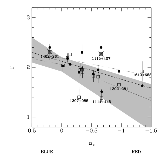
Figure 8: Plot of $\Gamma$ versus $\alpha_{\rm o}$ for BQS quasars in the XMM-Newton sample of Porquet et al. (2004). The open squares are the Porquet et al. (2004) 2–5 keV $\Gamma$ values from fitting XMM-Newton spectroscopic data; the filled circles indicate other spectroscopic X-ray measures of hard-band $\Gamma$ from the literature of some of the same quasars (see Appendix; Porquet et al. 2004). Dotted vertical lines connect datapoints for those quasars whose measures of $\Gamma$ differ by more than the given error bars. The values of $\alpha_{\rm o}$ were measured by Neugebauer et al. (1987) from continuum photometry. The ‘$\times$’ symbol indicates narrow-line quasars with H$\beta\,\rm FWHM<2000$ km s^-1. Narrow-line quasars, quasars with large $\Gamma$ variability, and outliers have been labeled for reference. PG 1114$+$445 has complex, intrinsic absorption that complicates the determination of $\Gamma$; George et al. (1997) measure $\Gamma=1.8\pm 0.1$. The dashed and dotted lines indicates the BCES estimator linear fit to the correlation of the average $\Gamma$ to $\alpha_{\rm o}$. The gray polygon marks the BCES estimator linear fit to the data for the SDSS sample plotted in Fig. 3d.

With a modest amount of Chandra exposure, we have derived some insight into the connection between X-ray and UV spectral properties of luminous quasars. From joint-spectral fitting, we have found that the quasars with large blueshifts ($\Delta v_{\rm b}\gtrsim 1100$ km s^-1) in our sample show significant evidence for intrinsic absorption with ${N}_{\rm H}$$\sim 10^{22}$ cm^-2 (assuming neutral gas with solar abundances). For this sample, unlike with samples of low $z$ or BAL quasars, $\Gamma_{\rm HR}$ is not a sensitive absorption indicator. The combination of column density (${N}_{\rm H}$$\sim 10^{22}$ cm^-2) and redshift pushes the energy cutoff from absorption to observed-frame $\sim 0.8$ keV (see Fig. 4). The effective area of ACIS S3 peaks between 1–2 keV, after the spectrum has recovered. The low-energy curvature of the power-law spectrum from absorption is thus only evident with the additional energy resolution utilized in joint-spectral fitting. These same factors, bandpass, redshift, and column density, also make $\alpha_{\rm ox}$ a weak indicator of intrinsic absorption for this sample, unlike for the ROSAT survey of low-redshift BQS quasars by Brandt et al. (2000). For that sample, $\alpha_{\rm ox}$ $\lesssim-2.0$ was a strong predictor of comparable column densities of X-ray absorption (Gallagher et al. 2001). Unfortunately, the BQS sample cannot be used effectively to study X-ray absorption in large-blueshift quasars. Of luminous ($M_{V}<-24$), radio-quiet BQS quasars with measured blueshifts (Baskin & Laor 2004b), only two would qualify for our large-blueshift sample with $\Delta v_{\rm b}\gtrsim 1100$ km s^-1. The first, PG 1259$+$593 ($\Delta v_{\rm b}=3304$ km s^-1), was not detected with ROSAT, and Brandt et al. (2000) measured an upper limit on $\alpha_{\rm ox}$ of $-1.79$, which is (at least) moderately X-ray weak. For the second, PG 1543$+$489 ($\Delta v_{\rm b}=2032$ km s^-1), George et al. (2000) find their preferred spectral model for the ASCA data to include intrinsic absorption (${N}_{\rm H}$$=0.7\times 10^{21}$  cm^-2 for neutral gas) which may be ionized. Though the X-ray properties of these two quasars suggest that both may harbor intrinsic absorbers, the quality of the existing X-ray data is not sufficient for such a claim. Our second result is that $\Gamma_{\rm HR}$ correlates with $\alpha_{\rm uv}$. This might be expected if smaller values $\Gamma_{\rm HR}$ were tracing intrinsic absorption. Instead, the results from joint-spectral fitting indicate that the $\Gamma_{\rm HR}$–$\alpha_{\rm uv}$ trend seen in Figure 3d is not driven by absorption: instead the bluest quasars with the largest $\Gamma_{\rm HR}$ values show evidence for absorption. The correlation indicates an inherent difference in the actual X-ray photon index as a function of color, with redder quasars having harder X-ray spectra. Given that our sample is small and the statistical errors in the X-ray spectral properties are large, we investigated the connection between optical/UV continuum color and $\Gamma$ further with additional data from Porquet et al. (2004, hereafter P04). P04 systematically analyzed BQS X-ray spectra from the XMM-Newton archive. Many of these quasars also have measurements of their optical/UV continuum slopes, $\alpha_{\rm o}$, from power-law fits to narrow-band optical photometry by Neugebauer et al. (1987). For comparison with our results, the P04 sample was stripped of all radio-loud quasars and all quasars more than 2 magnitudes less luminous than PG 0953$+$396, the most luminous radio-quiet quasar in the sample ($M_{V}=-25.65$; Table 1 of P04), because both radio-loudness and luminosity might influence X-ray properties. The resulting range of optical luminosity matches that of our sample, though our sample is significantly more luminous overall (see column 5 of Table 1). Of the 16 remaining quasars, 14 had measurements of $\alpha_{\rm o}$. In Figure 8, we plot the observed-frame 2–5 keV $\Gamma$ measured by P04 versus $\alpha_{\rm o}$ from Neugebauer et al. (1987). Many of these quasars have additional hard-band $\Gamma$ measurements from spectral fits to different data (see the Appendix of P04 and reference therein), and we plot these as well with filled circles. Several quasars (PG 1202$+$281, 1307$+$085, 1353$+$183, and 1613$+$658) show significant differences in $\Gamma$ between observations, which may result from actual variability and/or differences in analyses or observatories. There is clearly a large scatter, but the general trend that the bluest quasars have the steepest hard-band X-ray spectra is consistent with our results. For the filtered P04 sample, the Spearman and Kendall probabilities of no correlation between $\Gamma$ and $\alpha_{\rm o}$ are 0.038 and 0.028, respectively. If the averages between the P04 and previous values are used, the no-correlation probabilities are 0.022 and 0.014 for the same sample. The BCES estimator linear fit to the average $\Gamma$–$\alpha_{\rm o}$ datapoints is overplotted in Figure 8. To compare directly the BQS data to the data plotted in Figure 3d, a polygon encompassing the 1$\sigma$ range in slope and intercept for the linear fit is overplotted in Figure 8. The two independent fits are consistent within the 1$\sigma$ errors in both slope and intercept. Neither of these results relating hard-band $\Gamma$ to optical/UV color is independently conclusive, but the combined evidence from the $\Gamma_{\rm HR}$–$\alpha_{\rm uv}$ trend and the presented BQS data points to a consistent picture. The hard-band X-ray and optical/UV continua are linked; the bluer quasars exhibit steeper X-ray spectra.

6 Discussion

The observation that the large-blueshift quasars are blue in the optical/UV (Figure 6b) and have higher intrinsic absorption column densities (Figures 5 and 7) is consistent with large blueshifts occurring in quasars observed close to the plane of the accretion disk. In particular, the models of Hubeny et al. (2000) predict (their Fig. 12) that edge-on accretion disks are bluer than face-on disks. Such large inclination angles with respect to the disk normal would be expected to yield larger X-ray absorption column densities if the absorbing material is found closest to the disk. This scenario would also be consistent with the idea that BAL quasar outflows (known to have significant absorption in both the UV and X-ray) are equatorial. In addition, Reichard et al. (2003) suggest that BAL quasars are also intrinsically blue. If we extend this connection, large-blueshift quasars may have orientation angles close to those of BAL quasars that do not actually intercept the UV-absorbing wind. The absence of significant C IV absorption in the large-blueshift quasars indicates that the X-ray absorbing gas is either highly ionized (with little UV opacity) and/or does not obscure the UV continuum. The fraction of carbon ionized less than C V drops to $<1\%$ in a photoionized plasma with $\xi\gtrsim 8$  erg cm s^-1(where $\xi=L/nR^{2}$ [$L$ is the integrated luminosity from 1 to 1000 ryd, $n$ is the gas density, and $R$ is the distance from the radiation source]; Kallman & Bautista 2001). At this ionization parameter for $z\sim 2$, the actual column density of solar metallicity gas giving the same opacity in the observed Chandra bandpass as 1.5$\times 10^{22}$ cm^-2 of neutral gas is $\sim 50\%$ larger. The X-ray absorption seen in the large-blueshift quasars could be identified with the shielding gas postulated by Murray et al. (1995). This gas is required in their model to prevent soft X-rays from over-ionizing the disk-wind gas. Without it, radiation pressure by UV resonance line photons cannot radiatively drive the wind to the high velocities seen in BAL quasars. If this interpretation is correct, these data suggest that the shielding gas may have a larger covering fraction than the BAL outflow, and the blueshifted C IV emission could be interpreted as a disk-wind signature. For reference, BAL quasars typically show power-law X-ray spectra ($\Gamma\sim 2$) with complex, intrinsic X-ray absorption of ${N}_{\rm H}$ $\gtrsim 10^{23}$ cm^-2 (Green et al. 2001; Gallagher et al. 2002). While the connection between extreme blueshift and X-ray absorption fits reasonably within the Murray et al. (1995) disk-wind paradigm as an effect of orientation, understanding the relation between $\alpha_{\rm uv}$ and $\Gamma$ is more complicated. It is important to distinguish between this survey and previous work with ROSAT that focused on the observed 0.1–2.0 keV spectral slope, typically of $z\lesssim$1 quasars. Correlations found with ROSAT (e.g., Puchnarewicz et al. 1996) are much more sensitive to small absorbing column densities, and could also be driven by the soft excess. The soft excess, undetectable with these data, can often be modeled as a thermal black body, and is believed to originate in the inner accretion disk. For more relevant comparisons, there are many claims in the literature of correlations with the 2–10 keV $\Gamma$ (e.g., Zdziarski et al. 1999; Reeves & Turner 2000; Dai et al. 2004; Wang et al. 2004). The claim of a correlation between $\Gamma$ and $L/L_{\rm Edd}$ of Wang et al. (2004) is the most intriguing in the context of our sample. Based on comparisons with black-hole binaries (e.g., zg04), one might expect that objects with high accretion rates relative to Eddington will have softer hard X-ray spectra and a UV component that is more dominated by the disk (and thus bluer). In contrast, lower accretion-rate objects will have harder X-ray spectra and may appear redder due to a weaker inner disk component to the big blue bump. This picture is grossly consistent with the correlation of $\alpha_{\rm uv}$ with $\Gamma$. Our two most significant results (the presence of intrinsic X-ray absorption at large blueshift and harder X-ray spectra correlating with redder colors) thus are consistent with both orientation and accretion rate effects (either independently or together). The two dimensional structure in the $\Delta(g-i)$–blueshift distribution (Fig. 6b) implies that this is (at least) a two parameter problem. The absorption seen in the X-ray spectra of the largest-blueshift objects suggests that we are looking “down the wind” in such objects; in other words, that they are observed at the most extreme inclination angles with respect to the disk normal possible for an optically thick wind before BAL signatures are manifested. Large-blueshift objects also tend to have weak C IV equivalent widths. Therefore, the association of 1) high accretion rates and small C IV equivalent widths (Baskin & Laor 2004a), 2) BAL quasars with bluer intrinsic spectra and large blueshifts (Reichard et al. 2003), and 3) BAL quasars with high accretion rates (Boroson 2002; Yuan & Wills 2003) means that the extreme population that shows bluer UV continua, large blueshift, weaker C IV, and absorbed X-ray spectra may represent the most extreme accretors with the largest inclination angles possible for a given wind geometry. Such a scenario would be qualitatively consistent with the narrowing of the color/blueshift distribution toward large blueshift velocities seen in Figure 6b. However, moving to less extreme blueshifts, the situation in this scenario gets complicated, because both objects with less powerful winds (because they are less luminous though still active accretors or because they are accreting less actively) at extreme angles and objects with very powerful winds at less extreme angles contribute. This leads to the stretch in the $\Delta(g-i)$ color distribution (the ordinate in Figure 6b), which is widest close to $\sim 0$ km s^-1 blueshift. Here we assume that the intrinsic $\Delta(g-i)$ color is a marker of Eddington accretion rate, with bluer continua resulting from higher accretion rates at a given orientation angle. This speculative interpretation of the two dimensional $\Delta(g-i)$–blueshift distribution can be tested with observing programs tuned to isolate the two phenomenological parameters, color and blueshift, in an attempt to map them onto the underlying physical drivers. In this interpretation, we conjecture that choosing a narrow range of color and luminosity would allow blueshift to be an orientation indicator, whereas choosing a range in blueshift and luminosity allows color to be an indicator of accretion rate (because this would remove any orientation dependence of the color). Alternately, Leighly (2004) suggests that blueshifted emission comes from a wind which arises in AGN only under certain conditions. If blueshifts always indicate the presence of winds, the histogram in Figure 6a implies that nearly all broad-line quasars have winds, and our detection of X-ray absorption in large-blueshift quasars is broadly consistent with this model. However, simply invoking a wind from the near face of an optically thick accretion disk to explain large C IV blueshifts (see also Elvis 2004) does not necessarily yield a simple shift, nor does it trivially explain the weakness of the lines found in large-blueshift quasars. Lastly, the relationship between the blueshifts and the C IV equivalent widths (EWs) deserves further discussion. Any successful model of the broad line region must account for both the blueshifts and the EWs of the emission lines. For example, it may be reasonable to unify the Baldwin (1977) effect and emission line blueshifts, especially given the findings by Richards et al. (2002) that the C IV blueshift effect is not apparently dominated by luminosity, by Baskin & Laor (2004a) that the Baldwin effect is driven by $L/L_{Edd}$ rather than $L$, and by Francis & Koratkar (1995) that the Baldwin effect is strongest in the red wing of the C IV emission line. Perhaps as $L/L_{Edd}$ increases, the greater dominance of radiative driving over gravity produces a faster wind with a larger opening angle relative to the disk normal. Such winds will cover less of the sky from the point of view of the continuum source, thereby intercepting less ionizing radiation and lowering the EW of C IV and other lines emitted by the wind.

7 Conclusions

From our analysis of Chandra ACIS observations of 13 radio-quiet SDSS quasars and their optical/UV spectral properties, we present the following conclusions:

• Those quasars in our sample with C IV blueshifts $\gtrsim 1100$ km s^-1 show evidence from joint-fitting of the X-ray spectra for intrinsic X-ray absorption with ${N}_{\rm H}$ $\sim 10^{22}$ cm^-2. We interpret the presence of X-ray absorption in the large-blueshift sample as support for the orientation interpretation of the C IV blueshift put forth by Richards et al. (2002) whereby large-blueshift quasars are seen at inclination angles close to the line of sight through the wind (which may have a range of opening angles). This result is broadly consistent with the disk-wind model of quasar broad-line regions of Murray et al. (1995).

• We find that there is a trend of steeper hard-band X-ray continua with bluer $\alpha_{\rm uv}$ spectral index in our sample; this result is supported by a complementary analysis of independent Bright Quasar Survey data from the literature. We find the Eddington accretion rate, $L/L_{\rm Edd}$, to be a likely candidate for the primary physical driver of this trend.

Extending this study to larger samples with higher-quality X-ray data is certainly warranted to test these claims. Specifically, given the lack of C IV absorption in the SDSS spectra of the large-blueshift sample, we predict that high quality X-ray spectroscopy will reveal this gas to be ionized with $\xi>8$ erg cm s^-1. With the large effective area and 0.3–10.0 keV bandpass, sensitive XMM-Newton observations could significantly constrain both the column density and ionization state of the absorption for each quasar in the large-blueshift sample. Furthermore, high signal-to-noise ratio X-ray observations of a quasar sample tuned to isolate the relationship between UV/optical and X-ray continua hold promise for understanding the effect of Eddington accretion rate on quasar spectral energy distributions.

Figure 1: Spectra of SDSS quasars with new Chandra observations. Dashed vertical lines indicate the expected peaks of C IV (1549.06Å) and Mg II  using the Mg II emission line to define the systemic redshift.

Figure 2: Spectra of SDSS quasars with archival Chandra observations.

Figure 3: Observed X-ray versus optical properties of the new (open circles) and archival (filled squares) C IV blueshift sample. (a) The value $\Delta\alpha_{\rm ox}$ versus C IV blueshift. The parameter $\Delta\alpha_{\rm ox}$ is the difference between the observed $\alpha_{\rm ox}$ and the expected $\alpha_{\rm ox}$ (calculated using the luminosity density at 2500 Å from Equation 4 of Vignali et al. 2003; see Table 3). The errors plotted are the errors in $\alpha_{\rm ox}$. (b) The value $\Delta\alpha_{\rm ox}$ versus $\Delta(g-i)$ color. The three solid lines represent the expected changes in $\Delta\alpha_{\rm ox}$ and $\Delta(g-i)$ from SMC reddenings of $E(B-V)$=0.018, 0.046, and 0.081. (c) The photon index calculated from the hardness ratio, $\Gamma_{\rm HR}$, versus blueshift. (d) $\Gamma_{\rm HR}$ versus $\alpha_{\rm uv}$. The dashed and dotted lines indicate the best-fitting linear correlation and 1$\sigma$ errors in the slope and intercept from the BCES estimator.

Figure 4: Chandra spectra of the combined large (filled circles) and small (crosses) blueshift samples. Both data sets have been fit with a power-law model above observed-frame 1 keV, and the models (solid histograms) have been extrapolated back to 0.5 keV. The residuals (lower panel) indicate that while a power-law model with $\Gamma\sim 1.4$ is an adequate fit to the small blueshift sample, a power law model with $\Gamma\sim 2.2$ overpredicts the counts between 0.5–1.0 keV for the large-blueshift sample. These negative residuals are the signature of intrinsic absorption.

Figure 5: Confidence contours of photon index, $\Gamma$, versus intrinsic ${N}_{\rm H}$ from joint-spectral fitting for the new plus archival large (thick solid curves; sample 3), moderate (thin solid curves; sample 4), and small (dotted curves; sample 5) blueshift samples as defined in Table 4. The contours are for 68$\%$ ($\Delta C=2.30$) and 90$\%$ ($\Delta C=4.61$) confidence.

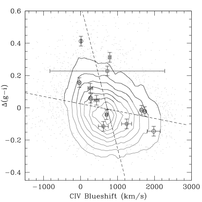
Figure 6: Left: Histogram of the distribution of C IV blueshifts from the SDSS DR2 quasar sample with C IV blueshift errors $<$250 km s^-1. The dotted vertical line marks the median blueshift value of the sample, and the dashed vertical line marks zero velocity. Right: Contour plot of the distribution of $\Delta(g-i)$ versus C IV blueshifts for the entire SDSS DR2 sample with $z$=1.54–2.20. Quasars with new observations are indicated with open circles and archival quasars with open squares. The dashed lines are the linear correlations from least-squares fits taking either color or blueshift as the dependent variable.

Figure 7: Results from X-ray joint-spectral fitting with absorbed power-law models: (a) $\Gamma$ and (ab) ${N}_{\rm H}$ versus C IV blueshift. Each datapoint indicates a small sample of quasars with a similar blueshift. The open symbols indicate spectra with enough X-ray counts to be fit individually. Errors in the ordinate are 1$\sigma$ taking two parameters to be of interest ($\Delta C=2.3$). For the jointly fit quasars (solid symbols), the abscissa value is the average of the quasars in each sample weighted by X-ray counts. Errors in the abscissa indicate the range (including uncertainties) of blueshift values in the objects contributing to each sample.

Table 1: Observed Targets

Name (SDSS J)	$z_{em}$	$i$	$M_{i}$	$\Delta v_{\rm b}$	$\Delta(g-i)$	$\alpha_{\rm o}$	$E$$($$B$$-$$V$$)$	${N}_{\rm H}$	Sample
000654.10$-$001533.4	1.720	17.829	$-27.18$	$-$33$\pm 28$	$0.156\pm 0.030$	$-0.09$	0.033	3.16	S/I
015650.28$+$005308.4	1.652	18.239	$-26.67$	11$\pm 15$	$0.413\pm 0.028$	$-1.25$	0.029	2.69	S/I
115115.38$+$003826.9	1.884	17.547	$-27.67$	270$\pm 28$	$0.060\pm 0.024$	$-0.46$	0.021	2.26	S/II
005102.42$-$010244.3	1.890	17.367	$-27.84$	1651$\pm 34$	$-0.014\pm 0.030$	$-$0.12	0.041	2.83	L/III
014812.23$+$000153.3	1.712	17.408	$-27.59$	1980$\pm 177$	$-0.145\pm 0.028$	$-0.02$	0.037	2.88	L/IV
020845.54$+$002236.0	1.900	16.734	$-28.49$	1738$\pm 35$	$-0.023\pm 0.035$	$-0.43$	0.027	2.78	L/IV
Archival Targets
003131.44$+$003420.2	1.732	18.425	$-26.62$	264$\pm 68$	$0.122\pm 0.038$	$-0.24$	0.024	2.41	S/II
173716.55$+$582839.4	1.775	18.595	$-26.49$	433$\pm 69$	$0.047\pm 0.023$	$-0.15$	0.042	3.51	S/II
234819.58$+$005721.4	2.160	18.611	$-26.93$	617$\pm 136$	$-0.115\pm 0.043$	$-0.14$	0.025	3.81	M/IND
011309.06$+$153553.5	1.809	17.839	$-27.28$	705$\pm 29$	$-0.042\pm 0.029$	$-$0.03	0.070	4.38	M/IND
124540.99$-$002744.8	1.687	18.157	$-26.83$	726$\pm 1552$	$0.228\pm 0.028$	$-0.58$	0.024	1.73	NA/NA
143841.95$+$034110.3	1.740	17.754	$-27.27$	788$\pm 36$	$0.313\pm 0.022$	$-1.20$	0.043	2.62	M/IND
120436.63$+$015025.6	1.936	18.395	$-26.88$	1247$\pm 136$	$-0.099\pm 0.030$	$-0.84$	0.026	1.88	L/III
020022.01$-$084512.1	1.942	18.283	$-27.02$	337$\pm 18$	$0.398\pm 0.033$	$\cdots$	0.024	2.12	NA

Table 2: Observing Log

Name	Obs. ID	Date (MJD)	$\theta$	Exposure	Counts		Count Rate	HR
(SDSS J)			(′)	Time (ks)	Soft	Hard	(10-3 ct  s-1)
000654.10$-$001533.4	4096	2003 Aug 02 (52853)	0.0	4.45	$34^{+6.9}_{-5.8}$	$9^{+4.1}_{-2.9}$	$9.88^{+1.73}_{-1.48}$	$-0.58^{+0.15}_{-0.13}$
015650.28$+$005308.4	4100	2003 Feb 23 (52693)	0.0	5.57	$55^{+8.5}_{-7.4}$	$34^{+6.9}_{-5.8}$	$15.97^{+1.88}_{-1.69}$	$-0.24^{+0.11}_{-0.11}$
115115.38$+$003826.9	4101	2003 Mar 03 (52701)	0.0	3.69	$38^{+7.2}_{-6.1}$	$11^{+4.4}_{-3.3}$	$13.29^{+2.18}_{-1.89}$	$-0.55^{+0.14}_{-0.12}$
005102.42$-$010244.3	4097	2002 Nov 20 (52598)	0.0	3.50	$42^{+7.5}_{-6.5}$	$9^{+4.1}_{-2.9}$	$14.56^{+2.34}_{-2.03}$	$-0.65^{+0.13}_{-0.11}$
014812.23$+$000153.3	4098	2003 Jun 25 (52815)	0.0	3.71	$24^{+6.0}_{-4.9}$	$2^{+2.7}_{-1.3}$	$7.29^{+1.69}_{-1.39}$	$-0.85^{+0.17}_{-0.10}$
020845.54$+$002236.0	4099	2003 Aug 26 (52877)	0.0	3.54	$40^{+7.4}_{-6.3}$	$11^{+4.4}_{-3.3}$	$14.39^{+2.31}_{-2.01}$	$-0.57^{+0.14}_{-0.12}$
Archival Targets
003131.44$+$003420.2	2101	2001 May 20 (52080)	1.0	6.69	$51.8^{+8.3}_{-7.2}$	$9.4^{+4.3}_{-3.1}$	$9.16^{+1.33}_{-1.17}$	$-0.69^{+0.12}_{-0.10}$
173716.55$+$582839.4	3038	2002 Aug 05 (52491)	3.7	4.62	$16.9^{+5.2}_{-4.1}$	$<5.4$	$4.09^{+1.18}_{-0.94}$	$<-0.52$
234819.58$+$005721.4	861	2000 May 26 (51691)	0.0	74.20	$285.9^{+18.0}_{-16.9}$	$45.1^{+7.9}_{-6.8}$	$4.46^{+0.26}_{-0.25}$	$-0.73^{+0.04}_{-0.04}$
011309.06$+$153553.5	3219	2002 Oct 18 (52565)	6.2	58.50	$390.0^{+20.9}_{-19.8}$	$117.4^{+12.0}_{-11.0}$	$8.67^{+0.41}_{-0.39}$	$-0.54^{+0.04}_{-0.04}$
124540.99$-$002744.8	4018	2003 Feb 14 (52684)	8.1	4.94	$64.4^{+9.1}_{-8.0}$	$23.0^{+6.0}_{-4.9}$	$17.69^{+2.12}_{-1.91}$	$-0.47^{+0.11}_{-0.10}$
143841.95$+$034110.3	3290	2002 Mar 13 (52347)	6.9	57.57	$218.8^{+15.9}_{-14.8}$	$75.3^{+9.9}_{-8.9}$	$5.11^{+0.32}_{-0.30}$	$-0.49^{+0.06}_{-0.05}$
120436.63$+$015025.6	3234	2002 Nov 24 (52603)	4.1	29.96	$103.7^{+11.5}_{-10.4}$	$28.2^{+6.6}_{-5.5}$	$4.40^{+0.43}_{-0.39}$	$-0.57^{+0.08}_{-0.08}$
020022.01$-$084512.1	3265	2002 Oct 02 (52549)	9.4	17.91	$36.5^{+7.1}_{-6.1}$	$15.6^{+5.2}_{-4.1}$	$2.91^{+0.47}_{-0.41}$	$-0.40^{+0.15}_{-0.14}$

Table 3: X-ray Properties

Name (SDSS J)	$\Gamma_{\rm HR}$	$\log(F_{\rm X})$	$\log(f_{\rm 2keV})$	SDSS MJD	$\log(f_{\rm 2500})$	$\log(L_{\rm 2500})$	$\alpha_{\rm ox}$	$\Delta\alpha_{\rm ox}$
000654.10$-$001533.4	1.85${}^{+0.42}_{-0.35}$	$-13.149\pm 0.070$	$-30.910\pm 0.070$	52519	$-26.736\pm 0.025$	$31.132\pm 0.025$	$-1.60\pm 0.09$	0.06
015650.28$+$005308.4	1.08${}^{+0.22}_{-0.20}$	$-12.751\pm 0.049$	$-30.955\pm 0.049$	51871	$-26.755\pm 0.018$	$31.079\pm 0.018$	$-1.61\pm 0.09$	0.05
115115.38$+$003826.9	1.75${}^{+0.35}_{-0.33}$	$-13.012\pm 0.067$	$-30.803\pm 0.067$	51943	$-26.626\pm 0.014$	$31.311\pm 0.014$	$-1.60\pm 0.09$	0.08
005102.42$-$010244.3	2.03${}^{+0.37}_{-0.36}$	$-13.033\pm 0.065$	$-30.685\pm 0.065$	52201	$-26.517\pm 0.016$	$31.422\pm 0.016$	$-1.60\pm 0.08$	0.09
014812.23$+$000153.3	2.90${}^{+0.90}_{-0.77}$	$-13.437\pm 0.092$	$-30.849\pm 0.092$	52199	$-26.554\pm 0.015$	$31.309\pm 0.015$	$-1.65\pm 0.11$	0.03
020845.54$+$002236.0	1.82${}^{+0.34}_{-0.34}$	$-12.984\pm 0.065$	$-30.734\pm 0.065$	52178	$-26.210\pm 0.014$	$31.734\pm 0.014$	$-1.74\pm 0.09$	$-0.02$
Archival Targets
003131.44$+$003420.2	$1.95^{+0.35}_{-0.35}$	$-13.294\pm 0.059$	$-31.009\pm 0.059$	51793	$-26.711\pm 0.025$	$31.163\pm 0.025$	$-1.65\pm 0.08$	0.02
173716.55$+$582839.4	$>1.45$	$-13.270\pm 0.113$	$-30.951\pm 0.113$	52017	$-26.890\pm 0.040$	$31.001\pm 0.040$	$-1.56\pm 0.14$	0.09
234819.58$+$005721.4	$2.07^{+0.17}_{-0.13}$	$-13.642\pm 0.025$	$-31.237\pm 0.025$	51788	$-26.968\pm 0.086$	$31.076\pm 0.086$	$-1.64\pm 0.04$	0.02
011309.06$+$153553.5	$1.88^{+0.10}_{-0.10}$	$-13.092\pm 0.020$	$-30.830\pm 0.020$	51878	$-27.039\pm 0.019$	$30.865\pm 0.019$	$-1.45\pm 0.07$	0.19
124540.99$-$002744.8	$1.62^{+0.25}_{-0.25}$	$-12.727\pm 0.050$	$-30.605\pm 0.050$	51928	$-27.099\pm 0.020$	$31.141\pm 0.020$	$-1.35\pm 0.09$	0.28
143841.95$+$034110.3	$1.73^{+0.12}_{-0.15}$	$-13.299\pm 0.026$	$-31.120\pm 0.026$	52023	$-26.734\pm 0.017$	$31.141\pm 0.017$	$-1.68\pm 0.06$	$-0.02$
120436.63$+$015025.6	$1.57^{+0.25}_{-0.25}$	$-13.503\pm 0.040$	$-31.387\pm 0.040$	52017	$-26.750\pm 0.101$	$31.207\pm 0.101$	$-1.78\pm 0.08$	$-0.11$
020022.01$-$084512.1	$1.48^{+0.32}_{-0.30}$	$-13.464\pm 0.066$	$-31.404\pm 0.066$	52149	$-26.833\pm 0.020$	$31.129\pm 0.020$	$-1.75\pm 0.09$	$-0.09$

Table 4: Results from Joint-Spectral Fitting

Sample	$\Gamma$	${N}_{\rm H}$	$C$-stat/$\nu$	Total
		(1022 cm-2)		Counts
1. Large – New (3)	$2.00^{+0.61}_{-0.62}$	$1.56^{+1.87}_{-1.53}$	426.8/1536	129
2. Small – New (3)	$1.42^{+0.35}_{-0.26}$	$0.00^{+0.86}_{-0.00}$	553.2/1536	180
3. Large – New (3) $+$ Archival (1)	$1.98^{+0.82}_{-0.29}$	$1.47^{+2.27}_{-0.93}$	648.2/2048	266
4. Small – New (3) $+$ Archival (2)	$1.64^{+0.32}_{-0.20}$	$0.00^{+0.63}_{-0.00}$	801.8/2560	260
5. Moderate – Archival (3)	$1.98^{+0.31}_{-0.13}$	$0.27^{+0.86}_{-0.27}$	996.9/1536	11391

References

- (1)
- Abazajian et al. (2004) Abazajian, K., et al. 2004, AJ, 128, 502
- Akritas & Bershady (1996) Akritas, M. G. & Bershady, M. A. 1996, ApJ, 470, 706
- Antonucci & Miller (1985) Antonucci, R. R. J. & Miller, J. S. 1985, ApJ, 297, 621
- Arnaud (1996) Arnaud, K. A. 1996, in ASP Conf. Ser. 101: Astronomical Data Analysis Software and Systems V, eds. G. Jacoby & J. Barnes, vol. 5, 17
- Baldwin (1977) Baldwin, J. A. 1977, ApJ, 214, 679
- Baskin & Laor (2004a) Baskin, A. & Laor, A. 2004a, MNRAS, 350, L31
- Baskin & Laor (2004b) — 2004b, MNRAS, submitted
- Bauer et al. (2004) Bauer, F. E., Alexander, D. M., N., B. W., Schneider, D. P., Treister, E., Hornschemeier, A. E., & Garmire, G. P. 2004, AJ, in press
- Becker et al. (1995) Becker, R. H., White, R. L., & Helfand, D. J. 1995, ApJ, 450, 559
- Boroson (2002) Boroson, T. A. 2002, ApJ, 565, 78
- Boroson & Green (1992) Boroson, T. A. & Green, R. F. 1992, ApJS, 80, 109
- Bouchet et al. (1985) Bouchet, P., Lequeux, J., Maurice, E., Prevot, L., & Prevot-Burnichon, M. L. 1985, A&A, 149, 330
- Brandt et al. (2000) Brandt, W. N., Laor, A., & Wills, B. J. 2000, ApJ, 528, 637
- Cash (1979) Cash, W. 1979, ApJ, 228, 939
- Dai et al. (2004) Dai, X., Chartas, G., Eracleous, M., & Garmire, G. P. 2004, ApJ, 605, 45
- Dickey & Lockman (1990) Dickey, J. M. & Lockman, F. J. 1990, ARA&A, 28, 215
- Elvis (2000) Elvis, M. 2000, ApJ, 545, 63
- Elvis (2004) — 2004, in ASP Conf. Ser. 311: AGN Physics with the Sloan Digital Sky Survey, eds. G. T. Richards & P. B. Hall, 109, astro-ph/0311436
- Francis & Koratkar (1995) Francis, P. J. & Koratkar, A. 1995, MNRAS, 274, 504
- Freeman et al. (2002) Freeman, P. E., Kashyap, V., Rosner, R., & Lamb, D. Q. 2002, ApJS, 138, 185
- Gallagher et al. (2002) Gallagher, S. C., Brandt, W. N., Chartas, G., & Garmire, G. P. 2002, ApJ, 567, 37
- Gallagher et al. (2001) Gallagher, S. C., Brandt, W. N., Laor, A., Elvis, M., Mathur, S., Wills, B. J., & Iyomoto, N. 2001, ApJ, 546, 795
- Gallagher et al. (1999) Gallagher, S. C., Brandt, W. N., Sambruna, R. M., Mathur, S., & Yamasaki, N. 1999, ApJ, 519, 549
- Garmire et al. (2003) Garmire, G. P., Bautz, M. W., Ford, P. G., Nousek, J. A., & Ricker, G. R. 2003, in Proceedings of the SPIE, Volume 4851: X-Ray and Gamma-Ray Telescopes and Instruments for Astronomy, eds. J. E. Trümper & H. D. Tananbaum, 28–44
- Gaskell (1982) Gaskell, C. M. 1982, ApJ, 263, 79
- Gehrels (1986) Gehrels, N. 1986, ApJ, 303, 336
- George et al. (1997) George, I. M., Nandra, K., Laor, A., Turner, T. J., Fiore, F., Netzer, H., & Mushotzky, R. F. 1997, ApJ, 491, 508
- George et al. (2000) George, I. M., Turner, T. J., Yaqoob, T., Netzer, H., Laor, A., Mushotzky, R. F., Nandra, K., & Takahashi, T. 2000, ApJ, 531, 52
- Green et al. (2001) Green, P. J., Aldcroft, T. L., Mathur, S., Wilkes, B. J., & Elvis, M. 2001, ApJ, 558, 109
- Green et al. (1995) Green, P. J., et al. 1995, ApJ, 450, 51
- Green et al. (2002) — 2002, ApJ, 571, 721
- Haardt & Maraschi (1993) Haardt, F. & Maraschi, L. 1993, ApJ, 413, 507
- Hewett et al. (1998) Hewett, P. C., Foltz, C. B., Harding, M. E., & Lewis, G. F. 1998, AJ, 115, 383
- Hopkins et al. (2004) Hopkins, P. F., et al. 2004, AJ, in press, astro-ph/0406293
- Hubeny et al. (2000) Hubeny, I., Agol, E., Blaes, O., & Krolik, J. H. 2000, ApJ, 533, 710
- Ivezić et al. (2002) Ivezić, Ž., et al. 2002, AJ, 124, 2364
- Ivezić et al. (2004) — 2004, in The Interplay Among Black Holes, Stars and ISM in Galactic Nuclei, eds. T. Storchi Bergmann, L. C. Ho, & H. R. Schmitt, in press, astro-ph/0404487
- Kallman & Bautista (2001) Kallman, T. & Bautista, M. 2001, ApJS, 133, 221
- Kraft, Burrows, & Nousek (1991) Kraft, R. P., Burrows, D. N., & Nousek, J. A. 1991, ApJ, 374, 344
- Krolik (2001) Krolik, J. H. 2001, ApJ, 551, 72
- Leighly (2004) Leighly, K. M. 2004, ApJ, astro-ph/0402452
- Leighly & Moore (2004) Leighly, K. M. & Moore, J. R. 2004, ApJ, in press, astro-ph/0402453
- Lyons (1991) Lyons, L. 1991, Data Analysis for Physical Science Students (Cambridge: Cambridge University Press)
- Marshall et al. (2004) Marshall, H. L., Tennant, A., Grant, C. E., Hitchcock, A. P., O’Dell, S. L., & Plucinsky, P. P. 2004, in Proceedings of the SPIE, Volume 5165: X-Ray and Gamma-Ray Instrumentation for Astronomy XIII., eds. K. A. Flanagan & O. H. W. Siegmund, 497–508
- Murray et al. (1995) Murray, N., Chiang, J., Grossman, S. A., & Voit, G. M. 1995, ApJ, 451, 498
- Neugebauer et al. (1987) Neugebauer, G., Green, R. F., Matthews, K., Schmidt, M., Soifer, B. T., & Bennett, J. 1987, ApJS, 63, 615
- Porquet et al. (2004) Porquet, D., Reeves, J. N., O’Brien, P., & Brinkmann, W. 2004, A&A, in press, astro-ph/0404385
- Puchnarewicz et al. (1996) Puchnarewicz, E. M., et al. 1996, MNRAS, 281, 1243
- Rao & Turnshek (2000) Rao, S. M. & Turnshek, D. A. 2000, ApJS, 130, 1
- Reeves & Turner (2000) Reeves, J. N. & Turner, M. J. L. 2000, MNRAS, 316, 234
- Reichard et al. (2003) Reichard, T. A., et al. 2003, AJ, 126, 2594
- Richards et al. (2004) Richards, G. T., Hall, P. B., Reichard, T. A., Berk, D. E. V., Schneider, D. P., & Strauss, M. A. 2004, in ASP Conf. Ser. 311: AGN Physics with the Sloan Digital Sky Survey, eds. G. T. Richards & P. B. Hall, 25, astro-ph/0312137
- Richards et al. (2002) Richards, G. T., Vanden Berk, D. E., Reichard, T. A., Hall, P. B., Schneider, D. P., SubbaRao, M., Thakar, A. R., & York, D. G. 2002, AJ, 124, 1
- Richards et al. (2003) Richards, G. T., et al. 2003, AJ, 126, 1131
- Richards et al. (2001) Richards, G. T., et al. 2001, AJ, 121, 2308
- Schmidt & Green (1983) Schmidt, M. & Green, R. F. 1983, ApJ, 269, 352
- Schneider et al. (2002) Schneider, D. P., et al. 2002, AJ, 123, 657
- Schneider et al. (2003) Schneider, D. P., et al. 2003, AJ, 126, 2579
- Stern et al. (1995) Stern, B. E., Poutanen, J., Svensson, R., Sikora, M., & Begelman, M. C. 1995, ApJ, 449, L13
- Tytler & Fan (1992) Tytler, D. & Fan, X. 1992, ApJS, 79, 1
- Vestergaard (2002) Vestergaard, M. 2002, ApJ, 571, 733
- Vignali et al. (2003) Vignali, C., et al. 2003, AJ, 125, 2876
- Wang et al. (2004) Wang, J., Watarai, K., & Mineshige, S. 2004, ApJ, 607, L107
- Weedman et al. (1982) Weedman, D. W., Weymann, R. J., Green, R. F., & Heckman, T. M. 1982, ApJ, 255, L5
- Weisskopf et al. (2002) Weisskopf, M. C., Brinkman, B., Canizares, C., Garmire, G., Murray, S., & Van Speybroeck, L. P. 2002, PASP, 114, 1
- Wilkes (1984) Wilkes, B. J. 1984, MNRAS, 207, 73
- York et al. (2000) York, D. G., et al. 2000, AJ, 120, 1579
- Yuan & Wills (2003) Yuan, M. J. & Wills, B. J. 2003, ApJ, 593, L11
- Zdziarski et al. (1999) Zdziarski, A. A., Lubinski, P., & Smith, D. A. 1999, MNRAS, 303, L11