Strong and weak lensing united II: the cluster mass distribution of the most X-ray luminous cluster RX~J1347.5$-$1145

We have shown that the cluster-mass reconstruction method which combines strong and weak gravitational lensing data, developed in the first paper in the series, successfully reconstructs the mass distribution of a simulated cluster. In this paper we apply the method to the ground-based high-quality multi-colour data of RX~J1347.5$-$1145, the most X-ray luminous cluster to date. A new analysis of the cluster core on very deep, multi-colour data analysis of VLT/FORS data reveals many more arc candidates than previously known for this cluster. The combined strong and weak lensing reconstruction confirms that the cluster is indeed very massive. If the redshift and identification of the multiple-image system as well as the redshift estimates of the source galaxies used for weak lensing are correct, we determine the enclosed cluster mass in a cylinder to $M(<360\>{\rm h}^{-1}\mbox{kpc})=(1.2\pm 0.3)\times 10^{15}M_{\odot}$. In addition the reconstructed mass distribution follows the distribution found with independent methods (X-ray measurements, SZ). With higher resolution (e.g. HST imaging data) more reliable multiple imaging information can be obtained and the reconstruction can be improved to accuracies greater than what is currently possible with weak and strong lensing techniques.

1 Introduction

Clusters of galaxies have been a focus of a very intense ongoing research. Especially important for many cosmological applications is a good determination of their mass. One way to obtain their masses is to use the gravitational lensing information, both from multiple image systems (strong lensing) as well as from distortions of background sources (weak lensing). Many weak and strong lensing cluster mass reconstructions have been successfully performed in the past (see e.g. Clowe & Schneider 2001, 2002, Gavazzi et al. 2004 for examples of weak lensing and e.g. Kneib et al. 2003, Smith et al. 2004 for a combination of weak and strong lensing). While weak lensing mass reconstructions have an advantage in constraining the mass at much larger radii than strong lensing, one of main limitations for both strong and weak lensing is the problem of the mass-sheet degeneracy (i.e. the mass profile of the cluster can only be determined up to a constant). In the absence of redshift information from individual sources and the lens, one can break this degeneracy only by making assumptions about the underlying potential. Different assumptions, however, can lead to discrepant results on the cluster mass. In this work we therefore use individual redshifts of background sources to overcome this problem. As shown in Bradač et al. (2004a), by using these and by extending the reconstruction to the inner parts of the cluster we are effectively able to break this degeneracy.

This is the second of the series of papers in which we develop and test a cluster mass reconstruction technique that combines strong and weak lensing information. In Bradač et al. (2004b) (hereafter Paper I) we describe the method in which we extend the weak lensing formalism to the inner parts of the cluster, use redshift information of the background sources and combine these with the constraints from multiply imaged systems. Using simulated data we have shown that the method is successful in reconstructing the mass distribution of a cluster, and yields an excellent agreement between the input and reconstructed mass also on scales within and beyond the Einstein radius.

Encouraged by the success of our method, we apply it to the weak and strong lensing data for the redshift $0.451$ cluster RX~J1347.5$-$1145 (Schindler et al. 1995), the most X-ray luminous cluster known to date. Due to its record holding, this cluster has been a subject of many studies in X-ray (Schindler et al. 1995, 1997, Allen et al. 2002, Ettori et al. 2004, Gitti & Schindler 2004) and optical (Fischer & Tyson 1997, Sahu et al. 1998, Cohen & Kneib 2002, Ravindranath & Ho 2002). It has also been detected through the Sunyaev-Zel’dovich effect (Pointecouteau et al. 2001, Komatsu et al. 2001, Kitayama et al. 2004). Yet the mass determinations based on X-ray properties, SZ effect, velocity dispersion measurement, strong and weak lensing have all yielded discrepant results (see Cohen & Kneib 2002 for a summary).

For the purpose of mass reconstruction we use VLT/FORS data on a field of $3.8\times 3.8\mbox{ arcmin}^{2}$ in U, B, V, R, and I bands. We also use Ks-band data from VLT/ISAAC to obtain more reliable photometric redshift estimates. The shape measurements for the weak lensing reconstruction is performed on two FORS bands, R and I. The strong lensing properties of this cluster are analysed. From previous data sets five arc candidates were reported (Schindler et al. 1995, Sahu et al. 1998); using the new multi-colour data we conclude that only two possibly belong to the same multiple image system. Furthermore, we searched for additional images belonging to this system and identified a third possible member. Several new arc candidates were found as well and are presented in this work. Particularly interesting is a very red arc candidate with two components, located at a distance of $1\mbox{ arcmin}$ from the brightest cluster galaxy (BCG). In addition, we detect further elongated structures, some of them have been previously indicated by Lenzen et al. (2004) who developed and use an automated arc searching routine.

This paper is organised as follows. In Sect. 2 we describe the observations and give a brief outline of the data reduction process. In Sect. 3 we describe how we search for multiply imaged systems. In Sect. 4 we give the results of a combined strong and weak lensing reconstruction and the cluster luminosity measurements. We conclude in Sect. 5.

2 Observations and data reduction process

The optical VLT data for the current project were obtained with ESO proposal 67.A-0427(A-C) (P.I. S. Schindler). The data was taken with FORS1 in the high-resolution mode (pixel scale $0.\!\!^{\prime\prime}09$; total field of view $\approx 3.\!\!^{\prime}2\times 3.\!\!^{\prime}2$) in service mode between April and September 2001. UBVRI Bessel filters were used in sub-arcsecond seeing conditions (see Table 1 for a summary of data properties). This allows us to estimate photometric redshifts for all galaxies and to support our mass and light analysis by a careful separation of foreground and background galaxies and cluster members (see below). Our primary band for the weak lensing analysis (the I) was taken in the 1-port read-out mode. Thus we avoid potential problems for object shape measurements due to varying noise properties in the central parts of the images. For the other 4 bands, primarily used for object photometry, the 4-port read-out mode was used. The data in each band consist of at least 20 individual exposures and were obtained with a dither pattern of $30.\!\!^{\prime\prime}0$ in RA and DEC in order to obtain clean coadded images of highest quality.

The data reduction was carried out with a pre-release version of THELI, a pipeline developed specifically for the processing of optical single- and multi-chip cameras (see Schirmer et al. 2003, Erben et al. 2005); here we only outline our astrometric calibration which is essential for weak lensing studies. First, we match object positions from I-band data with those from the USNO-A2 astrometric catalogue (Monet et al. 1998), which fixes the position of the individual exposures with respect to absolute sky coordinates and thus corresponds to a zero-order astrometric solution (”shift only”). Next, we used Mario Radovich’s Astrometrix (see McCracken et al. 2003 and http://www.na.astro.it/~radovich/WIFIX/) to fit image distortions by a two-dimensional, third-order polynomial. Hereby, the distances of the objects with coordinates in USNO-A2 catalogue and of the overlap sources in different images are minimised simultaneously in the $\chi^{2}$ sense. We end up with rms residuals of $\approx 0.\!\!^{\prime\prime}25$ for the USNO-A2 standard sources and $\approx 0.\!\!^{\prime\prime}01$ for the overlap objects. Afterwards, we extract high $S/N$ objects from the coadded I-band image which are used as astrometric standard sources (instead of USNO-A2) for the other bands. In all bands we achieve formally an internal astrometric accuracy of $\approx 0.\!\!^{\prime\prime}01-0.\!\!^{\prime\prime}015$ for the overlap sources. Most of the observations were done during photometric nights. Photometric zeropoints were deduced from the images of standard stars obtained as part of the standard calibration plan of the FORS1 instrument and reduced in the same way as the science data. The obtained zeropoints are in good agreement with the general trend analysis of the FORS1 zeropoints. From non-photometric nights we only include images with a maximum absorption of 0.1 mag in the coaddition process which is performed with drizzle (Fruchter & Hook 2002).

In addition, we retrieved Ks VLT-ISAAC data (pixel scale $0.\!\!^{\prime\prime}1484$; field of view $\approx 2.\!\!^{\prime}5\times 2.\!\!^{\prime}5$) from the ESO science archive (proposal ID 67.A-0095(B)). The data was processed with the eclipse package (see Devillard 1997).

We create the catalogue of objects using SExtractor (Bertin & Arnouts 1996) in dual-image mode. The I-band image is used for detections and the images of the other bands are only used to measure the corresponding magnitudes. An object is considered detected if five adjacent pixels had a flux that exceeded the local sky noise level by a factor of three. All magnitudes quoted in this paper are in the Vega system. The photometric redshifts (using isophotal magnitudes for cluster members and aperture magnitudes for background sources; see below) of the objects were obtained using the HyperZ package (Bolzonella et al. 2000).

Table 1: Properties of the data used in this work. The $5\sigma$ limiting magnitudes were determined with SExtractor using an aperture of $2^{\prime\prime}$.

Filter	Exposure time (s)	Seeing (′′)	Limiting mag.
$U$	11310	0.97	25.4
$B$	4800	0.67	26.9
$V$	4500	0.62	26.5
$R$	6000	0.67	26.3
$I$	6750	0.57	25.6
$Ks$	$\approx 7200$	0.73	21.4

2.1 Cluster member catalog

Figure 1: The $m_{\rm B}-m_{\rm V}$ vs. $m_{\rm V}-m_{\rm I}$ colours for the galaxies in our field. Cluster members are selected to lie inside the polygon. BCG colours are given as a triangle. In addition we plot as crosses all the galaxies which have a photometric redshift estimate $0.4<z_{\rm phot}<0.5$.

For cluster members, due to their brightness and different sizes, we argue that it is best to use isophotal magnitudes to obtain accurate colour estimates. In Fig. 1 we plot the $m_{\rm B}-m_{\rm V}$ vs. $m_{\rm V}-m_{\rm I}$ colours for the galaxies in our field. To determine the colour cuts for the cluster member selection we first inspect the galaxies having I-band magnitude up to three magnitudes fainter than the BCG and with a distance to the BCG smaller than $1^{\prime}$. These are preferentially the cluster members and form a group around $m_{\rm V}-m_{\rm I}\sim 2$ and $m_{\rm B}-m_{\rm V}\sim 1.8$. Using this information we determine the following selection criteria for the cluster members

$$0.7\left(m_{\rm B}-m_{\rm V}+1\right)< m_{\rm V}-m_{\rm I} <0.7\left(m_{\rm B}-m_{\rm V}+1.9\right)$$

$$1< m_{\rm B}-m_{\rm V} <2\;,$$ (1)

and we also cut out all the objects having magnitudes brighter than the BCG. In Fig. 1 we plot colours for all galaxies in our field, the BCG colours (slightly bluer than most other members) are given as a triangle and the polygon indicates the selection criteria we use. In addition, to avoid biases toward red cluster members, we add to the catalogue the blue galaxies with photometric redshifts $0.4<z_{\rm phot}<0.5$ (denoted as crosses in Fig. 1). The final photometric redshift distribution of the cluster members is given in Fig. 2. The completeness of our catalogue is discussed in Sect.4.4.

An alternative approach would be to select the cluster members purely from the redshift information. However due to uncertainties in redshift estimation the redshift distribution of the members is relatively broad. With broad cuts in redshift space one can get, on the one hand, a contamination of blue, non-cluster members and on the other hand, some red cluster members might be missed due to an incorrect redshift determination. In the previously described method the situation is reversed. We have tested both selection criteria to calculate the cluster luminosities (see Sect. 4.4) and both give comparable results.

To obtain absolute rest-frame I- and R-band magnitudes for the cluster members we determine the appropriate K-correction $K_{\rm I,R}(z)$ for the cluster (deflector) redshift $z_{\rm d}=0.451$ elliptical galaxies and FORS1 filters using the GISSEL library (Bruzual A. & Charlot 1993) and obtain $K_{\rm I}(z_{\rm d})=0.378$, $K_{\rm R}(z_{\rm d})=0.747$. In addition we apply galactic extinction $A_{\rm I,R}$ to the measured isophotal magnitudes and assume zero evolutionary correction. We use $A_{\rm I}=0.121$, and $A_{\rm R}=0.166$ from NED, where the values are obtained from Schlegel et al. (1998) and Cardelli et al. (1989).

Figure 2: The photometric redshift distributions of the cluster members selected as described in Sect. 2.1.

2.2 Background galaxy catalog

In contrast to the procedure we describe above, we use aperture magnitudes for the redshift determination of the background sources. The reason for using aperture instead of isophotal magnitudes is that for faint, noisy sources an estimate for the true object isophote is hard to achieve and can bias our results for these sources. The diameter of the aperture is set to twice the value of the seeing given in Table 1. In principle, one should degrade all the images to match the seeing of the worst one (in our case U). However, the effect is negligible compared to the photometric errors in the U-band, and therefore we compensate for that by choosing different sizes of the aperture.

For the weak lensing analysis the R- and I-band exposures were used. As outlined in Sect. 2, the I-band serves as our primary weak lensing science frame. It is the image with the highest number-density of sources that can be used for weak lensing. Below, we cross-check our results obtained in this band with a parallel analysis in the R-band. We correct all galaxies in the field for the PSF anisotropy and PSF smearing as described in Erben et al. (2001). The procedure is based on the KSB algorithm (Kaiser et al. 1995), in particular we use the IMCAT implementation (http://www.ifa.hawaii.edu/~kaiser). We select stars from the half-light-radius vs. magnitude diagram and fit a second-order polynomial to their measured ellipticities. In Fig. 3 we plot the measured PSF variation for the I- and R-band data.

Figure 3: The upper panels show the spatial variation of the PSF anisotropy in I (34 stars) and R (32 stars). The length of the sticks give the amplitude of the stellar ellipticities (the length corresponding to $\left|\epsilon\right|=0.01$ is given at the top-left). The maximum ellipticity is around 2%. The lower panels show the ellipticity distribution after correction with a second-order polynomial. The formal residuals are about 0.005 in each component. Because of the small field of view and the small number of stars, the true errors are probably higher but difficult to estimate.

For the final weak lensing catalogue only sources having photometric redshift estimate $z_{\rm phot}>0.55$ are considered. We end up with $N_{\rm g}=210$ background sources for the I-band data (giving 15 galaxies per $\mbox{arcmin}^{2}$), and with $N_{\rm g}=140$ ($10\mbox{ arcmin}^{-2}$) for the R-band. The resulting redshift distributions for both catalogues are given in Fig. 4, the mean photometric redshift of the samples are $\left\langle z_{\rm I}\right\rangle=1.18$ and $\left\langle z_{\rm R}\right\rangle=1.14$.

(a)

(b)

Figure 4: The redshift distributions of background sources used for weak lensing analysis (only sources with $z_{\rm phot}>0.55$ were considered) for I-band a) and R-band catalogue b). The mean photometric redshift of the samples is $\left\langle z_{\rm I}\right\rangle=1.18$ and $\left\langle z_{\rm R}\right\rangle=1.14$.

3 Searching for multiply imaged candidates of RX~J1347.5$-$1145

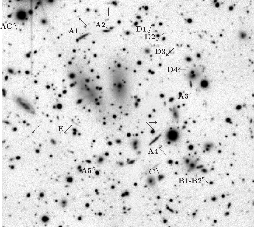
Figure 7: The $2.7\times 2.4\mbox{ arcmin}^{2}$ combined UBVRIKs image of the RX~J1347.5$-$1145 showing previously known (system A and C) and newly discovered (systems B, D, and E) arc candidates (see Table 2). All are marked with a label and an arrow, further arc candidates are marked with an arrow only. The image was scaled non-linearly and the scaling varies across the field (in order to enhance the details of the image).

Thus far, five arc candidates for this cluster have been reported in the literature. The first two were discovered by Schindler et al. (1995), and shallow HST STIS images revealed three additional ones (Sahu et al. 1998). These five arcs (A1-A5 as labelled by Sahu et al. 1998, see Fig. 7) are not all images of the same source. As is obvious from Fig. 6 most of them have different colours and surface brightnesses. Since gravitational lensing conserves both they belong to at least three different sources. However, two of these arcs (A4 and A5) do have the same colours and we consider them to be images of the same source. Although A4 has the appearance of a very straight, edge-on spiral galaxy (see Fig. 7), it can still be lensed, since the cluster members to the south west of it can produce a sufficiently strong tidal field to cause such a morphology. We note that the arc A3 considered by Allen et al. (2002) to belong to this system as well has different colours (see Table 3). Judging by the Fig. 6 one would think that A1 and A3 are multiple images of a single source as well, however the figure is a composite of 3 bands only and the detailed photometry shows that this is not the case(see Table. 3).

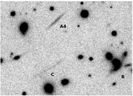
Figure 8: A $\sim 1.\!\!^{\prime}0\times 0.\!\!^{\prime}6$ cutout of the Ks-band image of RX~J1347.5$-$1145 showing one of the arcs used for strong lensing, the newly discovered very red arc system B1-B2 (two images almost merging, c.f. Fig. 6) and the long thin arc C.

We detect new arc candidates using the I-band and Ks-band image, as well as the combined (following the procedure described in Szalay et al. 1999) UBVRIKs image. In individual bands some of the arcs could not be significantly detected. In particular, we report here on the discovery of a red double-component arc candidate to the south-west of A4, which we designate with labels B1 and B2. The two components formed in the middle of a concentration of cluster members. Their extreme red colour suggests that it is either a highly reddened galaxy at $z\sim 1$ or it is a galaxy at $z\gtrsim 5$. In addition we detect in the vicinity of the system B a long thin arc candidate (C), which was also presented in Lenzen et al. (2004) as number 3 (see Fig. 8). In the vicinity of A2 we detect additional four arc candidates and denote them as D1-D4 (see Fig. 7). However, we do not claim that these components components belong to the same multiply imaged system, although their configuration is suggestive for that. Since these candidates are very faint, no reliable photometry can be obtained; the same is true for the arc candidate E. We use SExtractor to measure the ellipticities of these arcs from the I-band (systems A, C), Ks-band image (system B, due to its extreme red colour), and combined UBVRIKs image (systems D, E; since they can not be significantly detected in individual bands) – see Table 2. We detect more possible arc candidates (labelled only with arrows in Fig. 7). They are at the limit of the detection level and therefore their associated errors are too large for them to be used for our analysis.

Table 2: The properties of the arcs A1-A5 and the candidate counter-image AC used in the strong lensing analysis of the cluster. We also present additional arc candidates (systems B, C, D, and E) – see also Fig. 7. The properties of systems A, and C are measured from the I-band, while B is measured from the Ks-band image, and D and E are measured from the combined UBVRIKs image. The positions and position angles are given with respect to the brightest cluster member; the position angle of $90^{\circ}$ means that the arc is tangentially aligned with the BCG. All are measured with SExtractor. Because of the proximity of B1 and B2 to a cluster member we can not measure their ellipticities accurately.

Arc	$\theta_{1}$ [arcmin]	$\theta_{2}$ [arcmin]	$\left|\epsilon\right|$	PA$[\rm deg]$
A1	$-0.3460$	$\phantom{-}0.4547$	$0.571$	$82.0$
A2	$-0.1253$	$\phantom{-}0.5103$	$0.505$	$79.1$
A3	$\phantom{-}0.6644$	$\phantom{-}0.0090$	$0.613$	$96.1$
A4	$\phantom{-}0.3314$	$-0.4980$	$0.713$	$99.8$
A5	$-0.2891$	$-0.7009$	$0.333$	$99.4$
AC	$-1.0241$	$\phantom{-}0.6509$	$0.327$	$65.8$
B1	$\phantom{-}0.7440$	$-0.6873$
B2	$\phantom{-}0.6971$	$-0.7653$
C	$\phantom{-}0.3299$	$-0.4985$	$0.735$	$99.8$
D1	$\phantom{-}0.1985$	$\phantom{-}0.4492$	$0.219$	$81.8$
D2	$\phantom{-}0.3023$	$\phantom{-}0.3688$	$0.283$	$80.31$
D3	$\phantom{-}0.3812$	$\phantom{-}0.2562$	$0.364$	$56.5$
D4	$\phantom{-}0.4771$	$\phantom{-}0.1162$	$0.488$	$106.5$
E	$-0.4048$	$-0.3581$	$0.552$	$108.97$

Table 3: The photometric properties of the arcs A1, A2, A4, A5, and the candidate counter image AC. Given are three colours ($m_{\rm B}-m_{\rm I}$, $m_{\rm V}-m_{\rm I}$, and $m_{\rm R}-m_{\rm I}$) in magnitudes (measured from the isophotal magnitudes), VRI peak surface brightnesses $S_{\rm V,R,I}$ (in magnitudes), and photometric redshifts. For A1-A5 we determine them using 6 bands, for AC Ks is not available. If objects belong to the same source the colours and surface brightnesses need to be conserved.

	$m_{\rm B}-m_{\rm I}$	$m_{\rm V}-m_{\rm I}$	$m_{\rm R}-m_{\rm I}$	$S_{\rm V}$	$S_{\rm R}$	$S_{\rm I}$	$z_{\rm phot}$
A1	$2.20\pm 0.07$	$1.78\pm 0.05$	$0.98\pm 0.05$	24.37	23.75	22.72	0.69
A2	$3.66\pm 0.09$	$2.51\pm 0.05$	$1.38\pm 0.05$	24.16	23.44	21.88	0.73
A3	$1.52\pm 0.07$	$0.96\pm 0.05$	$0.54\pm 0.05$	24.23	23.89	23.19	1.65
A4	$0.99\pm 0.07$	$0.81\pm 0.05$	$0.53\pm 0.05$	23.60	23.30	22.60	1.76
A5	$1.08\pm 0.07$	$0.88\pm 0.05$	$0.57\pm 0.05$	23.60	23.29	22.60	1.70
AC	$1.28\pm 0.07$	$0.88\pm 0.05$	$0.52\pm 0.05$	23.90	23.50	22.98	1.30

Starting from the most plausible candidate multiple image system A4-A5 we search for additional images belonging this system in an automated fashion. The aperture magnitudes of an image in either $N_{\rm f}=6$ or $N_{\rm f}=5$ filters $m_{i,f}$ are compared with the magnitudes $m_{j,f}$ of all other images in the field (where $i$ is in our case the index of A4 or A5). We use the $\chi^{2}$ approach

$$\chi_{i,j}^{2}=\sum_{f=1}^{N_{\rm f}}\frac{\left(m_{i,f}-\left(m_{{j},f}+\mu_{i,j}\right)\right)^{2}}{\sigma_{i,f}^{2}+{\sigma_{j,f}^{2}}}\;,$$ (2)

where $\mu_{i,j}$ is the relative magnification between the images $i$ and $j$, and $\sigma_{i,f}$ and $\sigma_{j,f}$ are the magnitude measurement errors. Since lensing is achromatic we can evaluate $\mu_{i,j}$ by forcing $\partial\chi_{i,j}^{2}/\partial\mu_{i,j}=0$ to hold. The resulting $\chi_{i,j}^{2}$ function follows a $\chi^{2}$-distribution with $N_{\rm f}-1$ degrees of freedom. The best fitting images are then further visually analysed and tested for the conservation of surface brightness. A possible counter image candidate to A4 and A5 was found, which we label with AC. All three are encircled dashed-yellow in Fig 6, their photometric properties (and the properties of A1-A3) are listed in Table 3.

Using six flux measurements in UBVRIKs for the redshift determination of A4 and A5 and five in UBVRI for the AC (it is located at the edge of the Ks-band image and therefore the Ks photometry is not reliable) we find that A4 and A5 are consistent with being at a source redshift of $z_{\rm s}\simeq 1.76$. Unlike for other background objects (see Sect. 2.2), we use isophotal magnitudes to obtain reliable redshifts for A4 and A5 here due to the large ellipticity of the arcs. The redshift determination is in agreement with Ravindranath & Ho (2002) who, based on the absence of the $O[II]$ line in their spectrum, predict the redshift of A4 to be $>1.04$. The redshift estimate of AC using 5 filters is $1.3$; however, also the redshift estimates of arcs A4 and A5 are $1.3$ if we use only 5 filters. All three probability distributions for the redshift estimates are very broad and the higher redshift of $1.76$ is consistent with the photometric data in all three cases. In the redshift regime $1.2<z<2$ the main features in the spectral energy distribution (Lyman break, Balmer break, etc.) lie outside of the optical bands and therefore the NIR photometry is important. We therefore use the estimated photometric redshift from UBVRIKs of $z_{\rm s}\simeq 1.76$ from now on. Unfortunately, the redshift estimate for the multiply imaged system can substantially influence the combined cluster mass reconstruction (the position of the critical curve changes with redshift). We investigate this effect in Sect. 4.3.

Within the errors, the three images have the same colours as well as the same surface brightnesses (see Table 3). In addition, the photometric redshift estimate (using 6 filters) is the same for A4 and A5. The colours and peak surface brightnesses of the counter image are also consistent, however due to its smaller apparent size its photometry is less reliable. There are more candidate multiple image systems in this field; they will be the subject of a future study.

4 Cluster mass reconstruction of RX~J1347.5$-$1145

In this section we present the mass modelling of the cluster RX~J1347.5$-$1145. We first give a short outline of the method, a full account of it can be found in Paper I.

4.1 Short outline of the method

The main idea behind the method is to parametrise the cluster mass-distribution by a set of model parameters, where this parametrisation is chosen as generic as possible. In our case we use the gravitational potential $\psi$ on a regular grid. We factorise the redshift dependence by the so-called “cosmological weight” function $Z(z)$, as defined in Paper I (see also Bartelmann & Schneider 2001).

We define the $\chi^{2}$-function

$$\chi^{2}(\psi_{k})=\chi_{\epsilon}^{2}(\psi_{k})+\eta R(\psi_{k})+\chi_{\rm M}^{2}(\psi_{k})\;.$$ (3)

where $\chi_{\epsilon}^{2}(\psi_{k})$ is the contribution from weak lensing and $\chi_{\rm M}^{2}(\psi_{k})$ from strong lensing. In addition, the regularisation $R(\psi_{k})$ with regularisation parameter $\eta$ is employed in order to penalise any models that would follow the noise pattern in the data. We minimise the $\chi^{2}$ function with respect to $\psi_{k}$ by solving the equation $\partial\chi^{2}(\psi_{k})/\partial\psi_{k}=0$. This is in general a non-linear set of equations, and we solve it in an iterative manner. We linearise this system and starting from some trial solution (i.e. $\kappa^{(0)}$, $\gamma^{(0)}$, and $\@vec{\alpha}^{(0)}$) we repeat the procedure until convergence is achieved. We showed in Paper I that different models used as a trial solution do not influence results significantly. We try to confirm this result by investigating different models here as well.

4.2 Initial conditions for the method

For the purpose of obtaining the initial values for $\kappa^{(0)}$, $\gamma^{(0)}$, and $\@vec{\alpha}^{(0)}$ we first investigate the signal from the averaged tangential ellipticities and fit these using the singular isothermal sphere SIS model (hereafter called IS scenario). The tangential ellipticities are given by

$$\epsilon_{\rm t}=-\Re\left[\epsilon\>\rm e^{-2{\rm i}\phi}\right]$$ (4)

where $\phi$ specifies the direction to the source galaxy with respect to the the brightest cluster galaxy (BCG). In Fig. 5 we plot the average tangential ellipticities versus projected radius $\left\langle\theta\right\rangle$ in radial bins centred on the BCG, containing 50 (35) galaxies each. Both, the I- and R-band data give comparable results. We note that the tangential ellipticity signal is still high at the edge of the field $\left\langle\epsilon_{\rm t}\right\rangle\sim 0.1$, thus making this data inaccessible for standard weak lensing techniques aiming to determine the mass, since on this relatively small field one cannot break the mass-sheet degeneracy by simply assuming $\kappa\sim 0$ at the field edges.

We fit an SIS profile to the individual tangential ellipticities (not binned), the model ellipticities are calculated using the redshifts of these sources. The resulting line-of-sight velocity dispersion is $\sigma_{\rm I,SIS}=950\pm 60\mbox{ kms}^{-1}$ for the I-band data and $\sigma_{\rm R,SIS}=960\pm 70\mbox{ kms}^{-1}$ for the R-band (both $1\sigma$ error bars). The tangential ellipticity as a function of radius for this model is plotted in Fig.5 (dashed line) for the average source redshifts of $\left\langle z_{\rm I}\right\rangle=1.18$ and $\left\langle z_{\rm R}\right\rangle=1.14$ (see Sect. 2.2). In addition, the absence of the lens is excluded with more than $10\sigma$ significance in both bands (all minimisations and error analysis in this subsection are performed using C-minuit from James & Roos 1975).

The line-of-sight velocity dispersion estimates are higher than the measured velocity dispersion from Cohen & Kneib (2002), and lower than previous weak lensing, strong lensing and X-ray measurements. However, in the optical it is evident that the cluster has a lot of structure and therefore the SIS profile does not describe the cluster adequately. It has at least two main components; in addition there is X-ray emission off-centred from the BCG. Furthermore, at the scales where we measure the profile, $\lesssim 400{h^{-1}}\mbox{ kpc}$, the profile of the cluster is probably not isothermal (see e.g. Navarro et al. 2004). Therefore, the values of $\sigma$ obtained in this manner should not be trusted, we only use them for one of the initial models for $\kappa^{(0)}$

(a)

(b)

Figure 5: Average tangential ellipticity $\left\langle\epsilon_{\rm t}\right\rangle$ vs. projected radius $\left\langle\theta\right\rangle$ in radial bins centred on the brightest cluster member containing 50 galaxies per bin for the I-band data a) and 35 galaxies for the R-band data b). The errors are obtained by randomising the phases of the measured ellipticities, while preserving their absolute values. 100 randomisations were performed. The dashed line shows the best-fit SIS profile to the unbinned data, for the I-band we obtain $\sigma_{\rm I,SIS}=950\pm 60\mbox{ kms}^{-1}$ and for the R-band $\sigma_{\rm R,SIS}=960\pm 70\mbox{ kms}^{-1}$ (both $1\sigma$ error bars). It is plotted here for the average source redshifts of $\left\langle z_{\rm I}\right\rangle=1.18$ and $\left\langle z_{\rm R}\right\rangle=1.14$. In the interval $0^{\prime}<\left\langle\theta\right\rangle\lesssim 0.\!\!^{\prime}25$ the expectation value of the observed ellipticity (for these models) is given by $1/g(\theta,z)^{*}$ and the tangential ellipticity profile has a steep gradient at $\left\langle\theta\right\rangle\simeq 0.\!\!^{\prime}1$ (for both bands) where $Z(\left\langle z_{\rm R,I}\right\rangle)\kappa=1$ [since $g=Z\gamma/\left(1-Z\kappa\right)$]. At $\left\langle\theta\right\rangle\gtrsim 0.\!\!^{\prime}25$ the expectation value of the observed ellipticity is given by $g(\theta,z)$.

Another possibility to obtain initial conditions is to use the multiple image information for the cluster. We perform a very rough analysis by using the data for the arc system A4-A5-AC (given in Table 2). In addition to the image positions we also use image ellipticities as constraints. The model consists of a non-singular isothermal ellipse (NIE) (Keeton & Kochanek 1998), given by

$$\kappa(\@vec{\theta^{\prime}})=\frac{b_{0}}{2\sqrt{\frac{1+\left|\epsilon_{\rm g}\right|}{1-\left|\epsilon_{\rm g}\right|}\left(r_{\rm c,nis}^{2}+(\theta^{\prime}_{1})^{2}\right)+(\theta^{\prime}_{2})^{2}}}\;,$$ (5)

where $\@vec{\theta}^{\prime}$ is calculated w.r.t. the major axis of the cluster surface mass density. We allow the centre of the cluster potential $\@vec{\theta}_{\rm cl}$, the scaling $b_{0}$, ellipticity $\left|\epsilon_{\rm g}\right|$, and the position angle $\phi_{\rm g}$ to vary. Following the prescription of Kneib et al. (1996) we also include the 10 brightest cluster members in the I-band to the mass model. They are modelled as non-singular isothermal spheres with a line-of-sight velocity dispersion $\sigma_{\rm nis}$ and core radius $r_{\rm c,nis}$ following

$$\sigma_{\rm nis} {}\propto L^{1/4}\;, r_{\rm c,nis} {}\propto L^{1/2}\;,$$ (6)

The proportionality constants were chosen such that the I-band magnitude $m_{I}=17.5$ galaxy would have $\sigma_{\rm sis}=300\mbox{ km\,s}^{-1}$ and $r_{\rm c,nis}=0.\!\!^{\prime}1$ (the BCG has $m_{I}=17.8$). We also fix the core radius of the cluster to $0.\!\!^{\prime}3$. These constants are not allowed to vary. The best fit model for this system has values of $\{\theta_{{\rm cl},1},\theta_{{\rm cl},2},b_{0},\left|\epsilon_{\rm g}\right|,\phi_{g}\}=\{-0.\!\!^{\prime}21,-0.\!\!^{\prime}10,0.\!\!^{\prime}97,0.3,0.8\}$.

We stress here that it was not our aim to obtain a detailed strong lensing cluster-mass model, since it will only be used for the initial values of reconstruction. The multiple image system used here is independently included in the non-parametric reconstruction. We have shown in Paper I (and also confirm this in Sect. 4.3) that the reconstruction depends little upon the details of the initial model we use; for this reason a detailed modelling is not needed. In particular, the precise choice of those parameters that we did not vary in the modelling is not very relevant in our case. For the same reason we also do not include additional multiply imaged candidates in the analysis.

Figure 6: The BRK colour composite of the $\sim 3\times 3.2\mbox{ amin}^{2}$ field of RX~J1347.5$-$1145. Overlaid is in white contours the combined weak and strong lensing mass reconstruction from Fig. 9a1. The contour levels are the same (the field here is smaller), we smooth them here using a Gaussian kernel characterised by $\sigma=5^{\prime\prime}$ for clarity of the plot. Yellow circles show the multiple image system we use. North is up and East is left.

4.3 Combined weak and strong lensing mass reconstruction of RX~J1347.5$-$1145

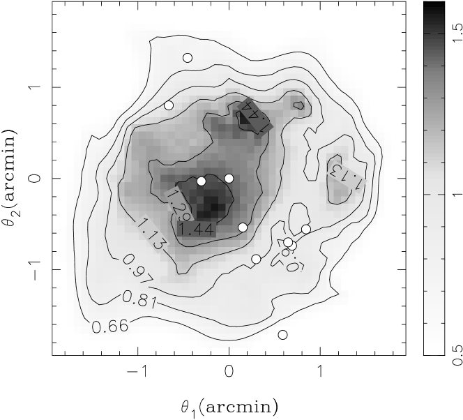
(a1)

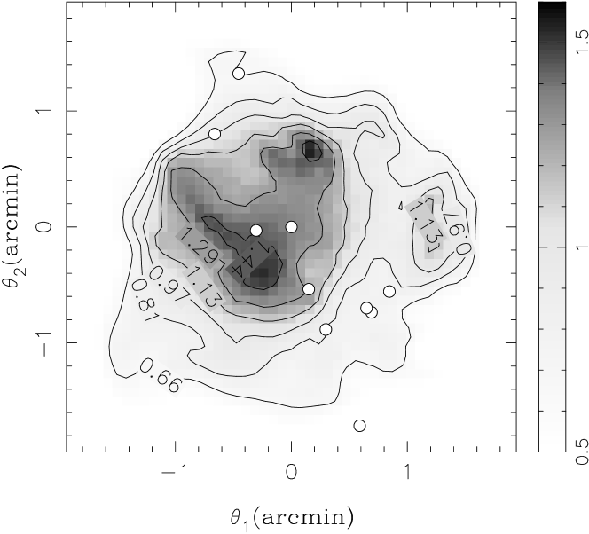
(b1)

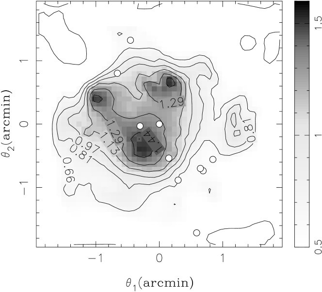
(c1)

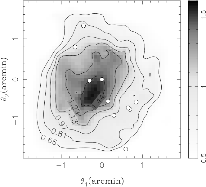
(a2)

(b2)

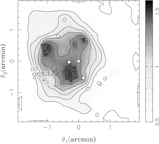
(c2)

Figure 9: $\kappa$-maps obtained from combined strong and weak lensing reconstruction of the cluster RX~J1347.5$-$1145. Left panels show the reconstructions using I-band data and for the ones on the right we use the R-band data. For the I-band data we have $N_{\rm g}=210$ background source galaxies, and for the R-band $N_{\rm g}=148$, all with known photometric redshifts. In a1) and a2) we use the best fit model from the strong lensing analysis of the cluster IM as initial condition, in b1) and b2) we use the IS model (SIS model fitted to tangential ellipticities, centred on the brightest cluster member) – for both IM and IS see Sect. 4.2. In c1 and c2) we use I0, i.e. $\kappa^{(0)}=0$ on all grid points. The positions of the 10 brightest cluster members are plotted as white circles.

We apply the mass-reconstruction method to the I- and R-band data of RX~J1347.5$-$1145 and the strong lensing system A4-A5-AC only (see Table 2). We use three different initial models for $\kappa^{(0)}$; IM is the best fit model from the strong lensing analysis of the cluster, the IS model is the best fit SIS model to binned tangential ellipticities (centred on the brightest cluster member) – both presented in Sect. 4.2 – and I0 has $\kappa^{(0)}=0$ ($\gamma^{(0)}=0$, $\@vec{\alpha}^{(0)}=\@vec{0}$). The initial regularisation parameter is set to $\eta=400$ for the I-band and $\eta=200$ for the R-band. It is adaptively adjusted in each iteration step such that the resulting $\chi^{2}/N_{\rm g}\sim 1$. The resulting $\kappa$-maps are given in Fig. 9. We also overlay the contours from Fig. 9a1 to the colour composite image in Fig. 6.

We estimate the mass within the cylinder of a radius of $1.\!\!^{\prime}5$ (for the cluster redshift $z_{\rm d}=0.451$ this corresponds to $360{h^{-1}}\mbox{ kpc}$), the estimates are given in Table 4. The projected mass of the cluster is estimated to be $M(<360\>{h}^{-1}\mbox{kpc})=(1.2\pm 0.3)\times 10^{15}M_{\odot}$. The error was estimated by bootstrap resampling the background galaxies in the weak lensing catalogues. This means that for each catalogue we randomly select $N_{\rm g}$ galaxies with replacement, if a galaxy is selected twice (or more) we assign double (or multiple) weight to its $\chi_{\epsilon}^{2}$ contribution. We generate 10 new catalogues and perform a new mass reconstruction; the error is then given as the variance of these estimates. It is larger than what we obtain from simulations in Paper I, which is partly attributed to the fact that we only use a three-image and not a four-image system here. However, within the given errors the results for both bands and for different initial models are consistent.

The projected mass from XMM measurements (Gitti & Schindler 2004) within a cylinder of the same radius as we use is given by $M_{\rm X}(<360\>{h}^{-1}\mbox{kpc})=(0.7\pm 0.2)\times 10^{15}M_{\odot}$ (Myriam Gitti, private communication). The resulting mass from the strong and weak lensing mass reconstruction is higher and marginally consistent with X-ray measurements. If the mass estimate is extrapolated at larger radii (assuming an isothermal profile) it is also consistent with the previous weak-lensing results by Fischer & Tyson (1997). It is however significantly larger than the mass estimate obtained by the velocity dispersion measurement of Cohen & Kneib (2002).

A possible explanation for the discrepant dynamical mass estimates was presented by Cohen & Kneib (2002). They argue that the cluster is most likely in a pre-merging process (with clumps merging preferentially in the plane of the sky). In such a scenario, until the merging is complete and the cluster is virialised, the dynamical cluster mass will be largely underestimated. On the other hand the X-ray temperature can be increased in such merging processes (thus the mass would be overestimated) and for this reason the south-east quadrant is excluded (the surface brightness profile is determined by averaging data only in the other three quadrants) in the X-ray analysis. The temperature measurements from Gitti & Schindler (2004) thus further supports the merger hypothesis. However if there is some extra mass present in the excluded quadrant (as suggested by our mass maps), the mass estimate obtained in this way from X-rays will be underestimated. If the hypothesis is correct, traditional mass estimates relying on equilibrium assumptions fail and gravitational lensing (with high quality data) provides the most accurate estimate for the cluster mass.

We note, however, that our results depend upon the correct redshift determination and identification of the members of the multiple image system we use. If we put the multiple image system to a redshift of $\sim 3$ ($\sim 1.3$), the estimated mass decreases (increases) by $\sim 10\%$. If the images do not belong to the same system, the changes might be even more drastic. However, at least for the two arcs A4 and A5, based on their photometric properties, we consider this possibility less likely (see Sect. 3). As a test we have also performed the reconstruction using only the two arcs A4 and A5. The results remain unchanged, however the scatter between the three initial models and the errors are larger by a factor $\sim 2$.

Further, the results rely on the correct determination of the photometric redshifts for the weak lensing sources. The random error of the determination is not crucial, the problem are the systematic uncertainties. It is not excluded that e.g. some foreground sources get assigned a high redshift and thus diluting (if they are randomly oriented) or enhancing the signal (if they are aligned). In addition, outliers can have $Z(z)$ assigned which is very different to their real cosmological weight. These outliers were considered in Paper I, they were chosen at random and their fraction was taken to be 10%. Still, their presence did not significantly change our conclusions. If, however, their fraction is higher and/or more importantly if they bias the final redshift distribution, this can bias our mass estimate.

An additional test for the accuracy and reliability of our model could be performed by using its predictive power. Namely, if the model is well constrained it should be capable of predicting the position of e.g. the counter image to the arc A1 (providing its redshift determination is correct). We have tested our models using the following procedure. Using the resulting potential from strong and weak lensing reconstruction we project (using bilinear interpolation and finite differencing) the position $\@vec{\theta}_{\rm s}$ of an arc candidate (e.g. A1) back to the source plane and denote the resulting position as $\@vec{y}_{\rm s}(\@vec{\theta}_{\rm s})$. Then we search for all possible solutions $\@vec{\theta}$ satisfying the non-linear set of equations $\@vec{y}(\@vec{\theta})-\@vec{y}_{\rm s}(\@vec{\theta}_{\rm s})=\@vec{0}$. These should then lie close to the possible counter image candidate(s). However, since our model is tightly constrained only in the vicinity of multiple images we use (A4, A5, and AC), the scatter of possible solutions is large. This issue could however be easily resolved in the future with e.g. ACS observations, since many more arc candidates will be found and their morphology can be obtained allowing for unambigous identification of multiple imaged systems and tighter constraints of the model.

Table 4: Reconstructed mass of RX~J1347.5$-$1145 within a cylinder of $360{h^{-1}}\mbox{ kpc}$ radius around the BCG from I-band (left) and R-band (right) weak lensing data and one candidate 3-image system. Three different $\kappa^{(0)}$ models have been used. We use the best fit model from the multiple image system IM, IS is the best fit SIS model from the process of parametrised fitting of weak lensing data and I0 has $\kappa^{(0)}=0$ on all grid points (see Sect. 4.2). In brackets we give for comparison the velocity dispersion of an SIS having the same enclosed mass within $360{h^{-1}}\mbox{ kpc}$.

	$M_{I}$	$[\sigma_{\rm I,SIS}]$	$M_{R}$	$[\sigma_{\rm R,SIS}]$
	$[10^{15}M_{\odot}]$	$[{\rm kms^{-1}}]$	$[10^{15}M_{\odot}]$	$[{\rm kms^{-1}}]$
IM	$1.37\pm 0.04$	[1900]	$1.31\pm 0.03$	[1860]
IS	$1.2\pm 0.1$	[1800]	$1.1\pm 0.1$	[1700]
I0	$1.1\pm 0.1$	[1700]	$1.1\pm 0.1$	[1700]

4.4 Rest-frame I- and R-band brightness distribution and mass-to-light ratio of RX~J1347.5$-$1145

(a)

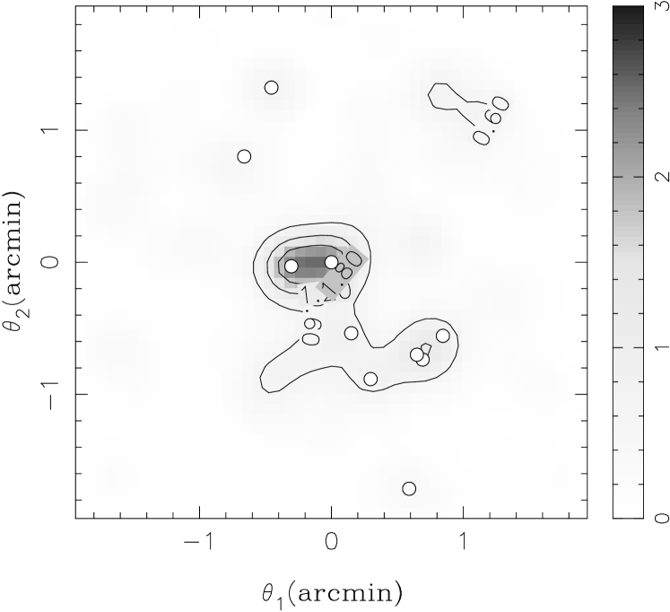
(b)

Figure 10: The I-band a) and R-band b) brightness distribution of the RX~J1347.5$-$1145 in $10^{12}L_{\odot}/\mbox{ arcmin}^{2}$. The cluster members are selected using the colour cuts described in the text, the ten brightest ones (in I) are plotted as white circles. Their luminosities of the cluster members have been smoothed using a Gaussian kernel characterised by $\sigma=9^{\prime\prime}$.

To obtain the cluster brightness distribution and aperture luminosity we proceed as follows. Using colour and redshift information for the selection criteria described in Sect. 2.1 we determine the luminosities of the cluster members in the field. They are smoothed using a Gaussian kernel characterised by $\sigma=9^{\prime\prime}$, resulting in the brightness distribution shown (for I-band only) in Fig. 10. We then determine the aperture luminosity $L_{\rm a}$ by adding the luminosities of the cluster members within $360{h^{-1}}\mbox{ kpc}$ radius around the BCG.

The resulting I- and R-band aperture luminosities are $L_{\rm a,I}(<360{h^{-1}}\mbox{kpc})=3.1\times 10^{12}L_{\odot}$ and $L_{\rm a,R}(<360{h^{-1}}\mbox{kpc})=2.2\times 10^{12}L_{\odot}$, respectively. The mass-to-light ratios (M/L) are $M/L_{\rm I}=400\pm 150M_{\odot}/L_{\rm I,\odot}$ and $M/L_{\rm R}=550\pm 150M_{\odot}/L_{\rm R,\odot}$. The cluster has only 300 members across the observed field, it is under-luminous in optical bands. In addition, we are measuring the M/L ratio in the inner part of the cluster, which might not reflect the M/L ratios measured out to $\sim 1\mbox{ Mpc}$ distances from cluster centres usually quoted in the literature.

The first concern with luminosity estimates is completeness. For this purpose we fit the Schechter luminosity function (Schechter 1976) to the cluster member counts as a function of absolute magnitudes $M_{\rm I}$ and $M_{\rm R}$. The resulting best-fit characteristic magnitudes are $M^{*}_{\rm I}=-22.4\pm 0.2$ and $M^{*}_{\rm R}=-21.7\pm 0.3$ and the faint end slopes are given by $\alpha_{\rm I}=-0.89\pm 0.06$, and $\alpha_{\rm R}=-0.9\pm 0.1$. We conclude that our catalogues are complete to a magnitude $M^{*}_{\rm I,R}-4$ and therefore the contribution from incompleteness is negligible.

A more severe concern is the contamination by non-cluster members and rejection of the actual members. In order to check against this, one needs to investigate the galaxy population “outside” the cluster region (on images taken with the same photometric conditions and depth as the images we use). A slightly different approach for the purpose of the M/L calculations can be followed by defining an outer aperture at the edge of the image and subtracting the luminosity density in that aperture from that in the inner portions of the cluster. The same approach needs to be undertaken when calculating the mass. If the M/L is constant across the field, this would give its correct value. Unfortunately our observed fields span only $\sim 450\mbox{ kpc}\>h^{-1}$ around the brightest cluster galaxy and therefore this approach is not reliable. We conclude that the error budget on luminosity is dominated by the systematics of the cluster member selection and contamination and is very difficult to estimate. We investigate two different selection criteria for cluster members in Sect. 2.1; we used colour information as well as the photometric redshifts. The aperture luminosities from these two criteria are consistent at the $5\%$-level. These two approaches share similar systematics, both use the same magnitude measurements, and for the colour-colour selection blue galaxies are added using photometric redshift measurements. However, in order to estimate the M/L the mass determination is a dominant source of error.

5 Conclusions

The case of RX~J1347.5$-$1145 has been a cause of many puzzles in the past. Very discrepant mass estimates are given in the literature, and unfortunately this cluster is not the only case where the mass measurements have proven to be difficult. We have applied a new mass reconstruction method to deep optical data using a multiple-image system with three images selected based on their colours and redshifts. Our main conclusions are the following.

1. The combined strong and weak lensing mass reconstruction confirms that the most X-ray luminous cluster is indeed very massive. If the redshift and identification of the multiple-image system, as well as redshifts used in weak lensing data, are correct we estimate the enclosed cluster mass within $360\>{h}^{-1}\mbox{kpc}$ to $M(<360\>{h}^{-1}\mbox{kpc})=(1.2\pm 0.3)\times 10^{15}M_{\odot}$.

2. The reconstruction shows a south-east mass extension, compatible with the X-ray measurements (see e.g. Gitti & Schindler 2004, Allen et al. 2002).

3. A single SIS fit to the average tangential ellipticities does not give a reliable estimate for the enclosed mass within $360\>{h}^{-1}\mbox{kpc}$; detailed modelling needs to be performed.

4. We have demonstrated the feasibility of breaking the mass-sheet degeneracy in practice by using shape measurements and adding the information on individual redshifts, without any assumptions regarding the cluster potential.

In addition we measured the corresponding mass-to-light ratio of the cluster within $360\>{h}^{-1}\mbox{kpc}$. We find that the cluster is more luminous in the rest-frame I-band than R-band, which is expected due to the presence of many old (red) elliptical galaxies in clusters. The resulting mass-to-light ratios are high, both in rest-frame I- and R-band, giving $M/L_{\rm I}=400\pm 150M_{\odot}/L_{\rm I,\odot}$ and $M/L_{\rm R}=550\pm 150M_{\odot}/L_{\rm R,\odot}$. These values are higher than typical values for clusters claimed in the literature ($\sim 200$ for R-band). However it is difficult to compare our results with existing measurements of the mass-to-light ratios, since they are usually performed at larger radii not accessible with our data.

In the course of this research we discovered one new extremely red arc candidate (system B) at $\sim 1\mbox{ arcmin}$ distance from the BCG. Unfortunately its redshift can not be measured, as it is significantly detected only in the Ks band. Further arc candidates are discovered from the combined colour image, suggesting that the cluster is indeed very centrally concentrated. In addition, the enclosed mass we obtain using the combined reconstruction also fits reasonably well the standard mass vs. X-ray luminosity relation (see Reiprich & Böhringer 2002), provided we assume the model to be isothermal (which for the same enclosed mass as our reconstructed model means $\sigma\simeq 1800\mbox{ kms}^{-1}$) to a radius of $r_{200}$ frequently used to determine the relation.

The mass-reconstruction of RX~J1347.5$-$1145 can be significantly improved. Deep HST imaging would greatly help in identifying and confirming new multiple-image systems, thus allowing more detailed modelling. In addition, not only the centre of the light for each of the arcs can be used as constraints, but also their morphology. As mentioned in Paper I, the reconstruction technique with adaptive grid at image positions can be used for these purposes. Further, spectroscopic redshifts need to be obtained for the multiple-image system candidates as well as for the cluster members (to obtain velocity dispersion measurements from a large sample). Deep, wide-field imaging data of this cluster will help us to improve the weak lensing constraints also at larger radii than presented here. A large number density of sources that can be used for weak lensing accessible by ACS ($\gtrsim$ $120\mbox{ arcmin}^{-2}$) would greatly improve the accuracy of the mass estimate and enable us to resolve substructures in the cluster. The details of the reconstruction can be used to reliably determine the cluster profile.

In conclusion, even without the best data quality that can be reached at present, we were able to perform a detailed cluster-mass reconstruction of the most X-ray luminous cluster RX~J1347.5$-$1145. The method has also shown a high potential for the future. If the highest quality data is used, a combination of strong and weak lensing has proven to offer a unique tool to pin down the masses of galaxy-clusters as well as their profiles and accurately test predictions within the CDM framework.