Strong and weak lensing united I: the combined strong and weak lensing cluster mass reconstruction method

Weak gravitational lensing is considered to be one of the most powerful tools to study the mass and the mass distribution of galaxy clusters. However, the mass-sheet degeneracy transformation has limited its success. We present a novel method for a cluster mass reconstruction which combines weak and strong lensing information on common scales and can, as a consequence, break the mass-sheet degeneracy. We extend the weak lensing formalism to the inner parts of the cluster and combine it with the constraints from multiple image systems. We demonstrate the feasibility of the method with simulations, finding an excellent agreement between the input and reconstructed mass also on scales within and beyond the Einstein radius. Using a single multiple image system and photometric redshift information of the background sources used for weak and strong lensing analysis, we find that we are effectively able to break the mass-sheet degeneracy, therefore removing one of the main limitations on cluster mass estimates. We conclude that with high resolution (e.g. HST) imaging data the method can more accurately reconstruct cluster masses and their profiles than currently existing lensing techniques.

1 Introduction

Clusters of galaxies have long been recognised as excellent laboratories for many cosmological applications. An especially important diagnostic is their number density as a function of mass and redshift. This can only be measured if reliable mass estimates of the observed clusters can be obtained. In addition, in the framework of the $\Lambda$CDM cosmological model, the dark matter distribution in clusters likely follows the NFW profile (Navarro et al. 1997).

Weak gravitational lensing is one of the most powerful tools currently available for studying the mass distribution of clusters of galaxies. The first weak lensing detection in clusters has been made by Tyson et al. (1990). However, it was only after the pioneering work by Kaiser & Squires (1993) that the field began to flourish, and since then many cluster mass reconstructions have been carried out (see e.g. Clowe & Schneider 2001, 2002, Gavazzi et al. 2004, Lombardi et al. 2005). A disagreement occurring in some cases between the cluster mass estimated from the weak/strong lensing measurements with X-rays is still not well understood, although several scenarios have been proposed to resolve this issue (see e.g. Allen 1998, Ettori & Lombardi 2003).

In the absence of the redshift information, the main limitation for a precise weak lensing mass estimate is the mass-sheet degeneracy (Schneider & Seitz 1995). If the redshifts of background sources and/or lens are not known, the transformation of the surface mass-density $\kappa\to\kappa^{\prime}=\lambda\kappa+(1-\lambda)$, where $\lambda\neq 0$ is an arbitrary constant, leaves the expectation value of measured image ellipticities unchanged. In Bradač et al. (2004b) we show that this degeneracy can be lifted using information on individual source redshifts, however only if the weak lensing reconstruction is extended to the critical parts of the cluster. Strong lensing is affected by this transformation as well. Namely, the mass-sheet degeneracy does not change the image positions (since the source position is not an observable) and flux ratios and therefore can not be broken if a single redshift multiple-image system is used. The mass-sheet degeneracy can in principle be broken using magnification effect (see Broadhurst et al. 1995, 2005). In order to make full use of this method, the unlensed source counts at a given magnitude threshold must be known accurately. Given the photometric calibration uncertainties, which at the faint magnitudes one is usually dealing with easily amount to $0.1\mbox{ mag}$, thus an uncertainty of $\sim 10\%$ in the unlensed source counts is typical. As shown by Schneider et al. (2000), this level of uncertainty removes a great deal of the power of the magnification method to break the mass-sheet degeneracy.

Several attempts have been made recently to measure the cluster mass profiles with weak lensing. However, as shown in Clowe & Schneider (2001, 2002), it is extremely difficult to distinguish e.g. isothermal from NFW profiles at high significance using weak lensing data alone. The authors also conclude that these difficulties mostly arise as a consequence of the mass-sheet degeneracy transformation. Therefore additional information needs to be included, such as combining the weak lensing data with strong lensing (see e.g. Kneib et al. 2003, Smith et al. 2004). Another example was given by Sand et al. (2004) using combined strong lensing and stellar kinematics data of the dominating central galaxy. This approach offers valuable extra constraints, however a detailed strong-lens modelling is required (Bartelmann & Meneghetti 2004, Dalal & Keeton 2003).

In this paper we use a combined strong and weak lensing mass reconstruction to determine the mass and the mass distribution of clusters. We reconstruct the gravitational potential $\psi$, since it locally determines both the lensing distortion (for weak lensing) as well as the deflection (for strong lensing). The method extends the idea from Bartelmann et al. (1996) and Seitz et al. (1998). Its novel feature is that we directly include strong lensing information. Further, weak lensing reconstruction is extended to the critical parts of the cluster and we include individual redshift information of background sources as well as of the source(s) being multiply imaged. This allows us to break the mass-sheet degeneracy and accurately measure the cluster mass and mass distribution. The method is tested using simulations, and in Bradač et al. (2004a) (hereafter Paper II) we apply it to the cluster RX J1347.5$-$1145. In this paper we first briefly present the basics of gravitational lensing in Sect. 2. In Sect. 3 we give an outline of the reconstruction method (detailed calculations are given in the Appendix). We test the method using N-body simulations, and we present the results in Sect. 4. The conclusions and summary are the subject of Sect. 5.

2 Gravitational lensing preliminaries

Throughout this paper we follow the notation of Bartelmann & Schneider (2001), who give a detailed account of the gravitational lensing theory presented here.

We start by considering a lens having a projected surface mass density $\Sigma(\@vec{\theta})$, where $\@vec{\theta}$ denotes the (angular) position in the lens plane. We define the dimensionless surface density $\kappa(\@vec{\theta})$ for a fiducial source located at a redshift $z\to\infty$ and a lens (deflector) at $z=z_{\rm d}$

$$\kappa(\@vec{\theta})=\frac{\Sigma(\@vec{\theta})}{\Sigma_{\rm cr}}\;\mbox{ where }\;\Sigma_{\rm cr}=\frac{c^{2}}{4\,\pi\,G}\frac{D_{\mathrm{\infty}}}{D_{\mathrm{d}}D_{\mathrm{d,\infty}}}\;.$$ (1)

$D_{\infty}$, $D_{\mathrm{d}}$, and $D_{\mathrm{d,\infty}}$ are the angular diameter distances between the observer and the source at $z\to\infty$, the observer and the lens, and the lens and the source, respectively. The choice of scaling with $\Sigma_{\rm cr}$ is motivated by the fact that lenses with $\Sigma\geq\Sigma_{\rm cr}$ (i.e. $\kappa\geq 1$) are strong enough to form multiple images. In this paper, however, strong lensing refers to multiple imaging only, while weak lensing means that the lensing effect is treated as statistical in nature, although it is also applied to the lens region with $\kappa>1$, traditionally called the strong lensing regime.

We define the deflection potential $\psi(\@vec{\theta})$

$$\psi(\@vec{\theta})=\frac{1}{\pi}\int_{\Re{}^{2}}{\rm d}^{2}\theta^{\prime}\,\kappa(\@vec{\theta}^{\prime})\,\ln|\@vec{\theta}-\@vec{\theta}^{\prime}|\;.$$ (2)

which is related to $\kappa$ via the Poisson equation

$$\nabla^{2}\psi(\@vec{\theta})=2\kappa(\@vec{\theta})$$ (3)

Also the shear $\gamma=\gamma_{1}+{\rm i}\gamma_{2}$ and the deflection angle $\@vec{\alpha}$ are related to $\psi$, where

$$\gamma_{1}=\frac{1}{2}(\psi_{,11}-\psi_{,22})\;,\quad\gamma_{2}=\psi_{,12}\;,\quad\@vec{\alpha}=\nabla\psi\;.$$ (4)

The relations (3) and (4) are written for the source at redshift $z\to\infty$; we note, however, that they hold for any redshift. Since we will work with sources at different redshifts (both for strong as well as for weak lensing), we factorise the redshift dependence of the lens convergence $\kappa$, the shear $\gamma$, and the deflection angle $\@vec{\alpha}$ by

$$\kappa(\@vec{\theta},z) {}=Z(z)\kappa(\@vec{\theta})\;, \gamma(\@vec{\theta},z) {}=Z(z)\gamma(\@vec{\theta})\;,$$

$$\@vec{\alpha}(\@vec{\theta},z) {}=Z(z)\@vec{\alpha}(\@vec{\theta})\;.$$ (5)

$Z(z)$ is the so-called “cosmological weight” function:

$$Z(z)\equiv\frac{D_{\infty}D_{\mathrm{d,s}}}{D_{\mathrm{d},\infty}D_{\mathrm{s}}}\,\mathrm{H}(z-z_{\mathrm{d}})\;,$$ (6)

where $D_{\mathrm{d,s}}$ and $D_{\mathrm{s}}$, are the angular diameter distances between the lens and the source, and the observer and the source at a redshift $z$, respectively. $\mathrm{H}(z-z_{\mathrm{d}})$ is the Heaviside step function and accounts for the fact that galaxies located at $z<z_{\rm d}$ are not lensed.

In the case of weak lensing, the information on the lens potential is contained in the transformation between the source ellipticity $\epsilon^{(s)}$ and image ellipticity $\epsilon$. It is given as a function of reduced shear $g(\@vec{\theta},z)$ (see Seitz & Schneider 1997)

$$\epsilon^{(s)}=\begin{cases}\dfrac{\epsilon-g(\@vec{\theta},z)}{1-g^{*}(\@vec{\theta},z)\epsilon}&\text{for $\bigl{\lvert}g(\@vec{\theta},z)\bigr{\rvert}\leq 1\;,$}\\[15.00002pt] \dfrac{1-g(\@vec{\theta},z)\epsilon^{*}}{\epsilon^{*}-g^{*}(\@vec{\theta},z)}&\text{for $\bigl{\lvert}g(\@vec{\theta},z)\bigr{\rvert}>1\;.$}\end{cases}$$ (7)

where

$$g(\@vec{\theta},z)=\frac{Z(z)\gamma(\@vec{\theta})}{1-Z(z)\kappa(\@vec{\theta})}\;.$$ (8)

Galaxies are intrinsically elliptical, and therefore one cannot disentangle the effect of lensing from the intrinsic properties in (7) using a single galaxy image. Hence, the weak lensing effect needs to be treated in statistical sense. More precisely, we can Taylor expand the expression (7) (e.g. for the case of $\left|g(\@vec{\theta},z)\right|\leq 1$) and recall that $\left|\epsilon^{(s)}\right|<1$ by definition to obtain

$$\epsilon(z) = \frac{\epsilon^{(s)}+g(\@vec{\theta},z)}{1+g^{*}(\@vec{\theta},z)\epsilon^{(s)}}$$ (9)

$$= \left(\epsilon^{(s)}+g(\@vec{\theta},z)\right)\sum_{k=0}^{\infty}(-1)^{k}(g^{*}(\@vec{\theta},z))^{k}(\epsilon^{(s)})^{k}\;.$$

A similar expansion can be obtained for the case $\left|g(\@vec{\theta},z)\right|>1$. If we assume that the intrinsic ellipticity distribution has moments $\bigl{\langle}{\epsilon^{(s)}}^{k}\bigr{\rangle}=0$ for each $k$ except $k=0$ we get the known expression for the expectation value of the image ellipticity at redshift $z$

$$\bigl{\langle}\epsilon(z)\bigr{\rangle}=\begin{cases}g(\@vec{\theta},z)&\text{if $\bigl{\lvert}g(\@vec{\theta},z)\bigr{\rvert}<1\ ,$}\\[10.00002pt] \frac{\displaystyle 1}{\displaystyle g^{*}(\@vec{\theta},z)}&\text{otherwise$\;.$}\end{cases}$$ (10)

This relation is particularly simple due to the convenient definition of $\epsilon$. In the approximation $\kappa\ll 1$, $\left|\gamma\right|\ll 1$ (thus $\left|g\right|\ll 1$) the expectation value is given by $\bigl{\langle}\epsilon(z)\bigr{\rangle}=\gamma(\@vec{\theta},z)$.

3 The cluster mass reconstruction method

The idea of combining strong and weak lensing constraints is not new, it has been previously discussed by Abdelsalam et al. (1998), Kneib et al. (2003), Smith et al. (2004), and others. The method presented here, however, has some important differences. For example in Abdelsalam et al. (1998) the authors reconstruct the pixelized version of the surface mass density $\kappa$. A similar method for strong lensing constraints only has recently also been presented by Diego et al. (2004). We argue, however, that using the potential $\psi$ is favourable, since $\kappa$, $\gamma$, and $\@vec{\alpha}$ locally depend upon the potential $\psi$ – c.f. (3), (4) – and all can be quantified from the latter. $\gamma$ and $\@vec{\alpha}$, on the other hand, are non-local quantities of $\kappa$. In other words, the mass density on a finite field does not describe the shear and the deflection angle in this field. If a finite field is used, one usually employs Fourier analysis; in this case, $\gamma$ in fact corresponds to original $\kappa$ plus all its periodic continuations.

Further, even though not easy to implement, we decided to keep the parametrisation of the mass-distribution as general as possible. In Kneib et al. (2003) and Smith et al. (2004), on the other hand, the strong and weak lensing constraints were compared in a Bayesian approach in the form of simple, parametrised models. In addition, the weak lensing constraints were not used to the very centre of the cluster and redshifts of individual sources were not included.

3.1 The outline of the method

The main idea behind the method is to describe the cluster mass-distribution by a fully general lens, using the values of the deflection potential $\psi$ on a regular grid. We then define a penalty function $\chi^{2}$ and minimise it with respect to the values of $\psi_{k}$. The convergence $\kappa$, the shear $\gamma$, and the deflection angle $\@vec{\alpha}$ at an arbitrary position in the field are obtained by finite differencing and bilinear interpolation methods. The number of grid points we use for $\psi_{k}$ is $(N_{\mathrm{x}}+2)\times(N_{\mathrm{y}}+2)$; the extension by one row and one column at each side is needed to perform the finite differencing at each inner $N_{\mathrm{x}}\times N_{\mathrm{y}}$ grid point.

We define the $\chi^{2}$-function as follows

$$\chi^{2}(\psi_{k})=\chi_{\epsilon}^{2}(\psi_{k})+\chi_{\rm M}^{2}(\psi_{k})+\eta R(\psi_{k})\;.$$ (11)

$\chi_{\epsilon}^{2}(\psi_{k})$ contains information from statistical weak lensing, whereas in $\chi_{\rm M}^{2}(\psi_{k})$ we include the multiple imaging properties. $R(\psi_{k})$ is a regularisation term multiplied by the regularisation parameter $\eta$. The regularisation is a function of the potential and disfavours small-scale fluctuations in the surface mass density.

In order to find the minimum $\chi^{2}$ solution, we solve

$$\frac{\partial\chi^{2}(\psi_{k})}{\partial\psi_{k}}=0\;.$$ (12)

This is in general a non-linear set of equations, which we solve in an iterative manner. We linearise this system and in the first step we start from some trial solution, to calculate its non-linear terms (see the Appendix for details). We solve the corresponding equations and repeat this procedure until a convergence is achieved. Inverting the resulting matrix of $\sim\left(N_{\mathrm{x}}\times N_{\mathrm{y}}\right)^{2}$ elements for finding a solution of the linear system is difficult in general even for grids with a small number of cells. However, as it turns out, the resulting matrix is sparse and the system is therefore computationally inexpensive to solve.

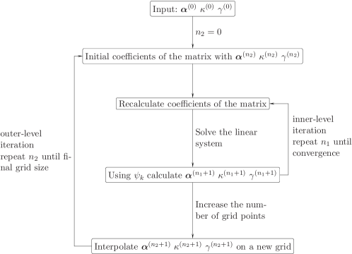
The reconstruction is performed in a two-level iteration process, outlined in Fig. 1. We will refer to the iteration process mentioned above for solving the linear system of equations as inner-level, where steps $n_{1}$ are repeated until convergence of $\kappa$. The outer-level iteration is performed for the purpose of regularisation (as described in detail in Sect. 3.3). In order to penalise small-scale fluctuations in the surface mass density, we start the reconstruction with a coarse grid (large cell size). Then for each $n_{2}$ step we increase the number of grid points in the field and compare the new reconstructed $\kappa^{(n_{2})}$ with the one from the previous iteration $\kappa^{(n_{2}-1)}$ (or with the initial input value $\kappa^{(0)}$ for $n_{2}=0$). The second-level iterations are performed until the final grid size is reached and convergence is achieved.

Figure 1: The outline of the two-level iteration process.

3.2 Technical aspects

In this section we will briefly describe some technical aspects of how we calculate the lensing quantities $\kappa$, $\gamma$, and $\@vec{\alpha}$ at an arbitrary position within the field from the potential $\psi_{k}$ on a grid.

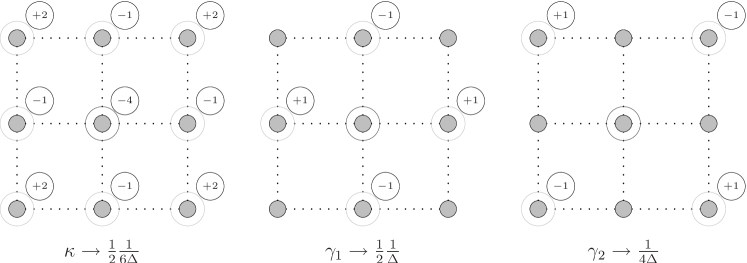
We use the finite differencing method with 9 grid points to calculate $\kappa$, 5 points for $\gamma$, and 4 points for $\@vec{\alpha}$ (see Abramowitz & Stegun 1972). The coefficients used for $\kappa$ and $\gamma$ are given in Fig. 2, the case of $\@vec{\alpha}$ is discussed in Appendix A.2. To evaluate $\kappa(\@vec{\theta})$, $\gamma(\@vec{\theta})$, and $\@vec{\alpha}(\@vec{\theta})$ at a position $\@vec{\theta}$ within the field, bilinear interpolation is used.

Note, that the dimensionality of the problem is not $(N_{\mathrm{x}}+2)\times(N_{\mathrm{y}}+2)$. Because the transformation $\psi(\@vec{\theta})\to\psi(\@vec{\theta})+\psi_{0}+\@vec{a}\cdot\@vec{\theta}$ leaves $\kappa$ and $\gamma$ invariant, the potential needs to be fixed at three points (see Seitz et al. 1998, Bartelmann et al. 1996). These thus fix the constant and linear term in the invariance transformation. If this is not the case, a minimum in $\chi^{2}$ would correspond to a three-dimensional subspace of possible solutions. The choice of the three points, and the corresponding values of the potential are arbitrary. Although the transformation $\psi(\@vec{\theta})\to\psi(\@vec{\theta})+\@vec{a}\cdot\@vec{\theta}$ changes the deflection angle $\@vec{\alpha}$, it only causes a translation of the source plane, which is not an observable. Therefore, even in the presence of strong lensing, three points of the potential need to be held fixed.

The mass-sheet degeneracy transformation of the potential is given by $\psi\to\psi^{\prime}=(1-\lambda)\@vec{\theta}^{2}/2+\lambda\psi$. However since we aim at lifting this degeneracy, in contrast to Seitz et al. (1998) the potential $\psi_{k}$, is not held fixed at an additional, fourth point. The dimensionality of the problem is thus $N_{\rm dim}=(N_{\mathrm{x}}+2)(N_{\mathrm{y}}+2)-3$.

Figure 2: The finite differencing coefficients for $\kappa$ (left), $\gamma_{1}$ (middle) and $\gamma_{2}$ (right). E.g. for $\kappa$ we use a formula including 9 points, the multiplicative factor is given at the bottom, the individual coefficients in the circle. Thus for the middle point $(0,0)$ we get $\kappa(0,0)=\frac{1}{2}\frac{1}{6\Delta}\big{[}2\left[\psi(-1,1)+\psi(1,1)+\psi(-1,-1)+\psi(1,-1)\right]-$ $\left[\psi(0,1)+\psi(-1,0)+\psi(1,0)+\psi(0,-1)\right]-4\psi(0,0)\big{]}$.

3.3 The $\chi^{2}$-function

In this section we will describe contributions to the $\chi^{2}$-function, starting with the statistical weak lensing.

For $N_{\mathrm{g}}$ galaxies with measured ellipticities $\epsilon_{i}$ we define the $\chi_{\epsilon}^{2}$ as

$$\chi_{\epsilon}^{2}(\psi_{k})=\sum_{i=1}^{N_{\mathrm{g}}}\frac{\left|\epsilon_{i}-\langle\epsilon\rangle\right|^{2}}{\sigma_{i}^{2}}\;,$$ (13)

where

$$\sigma_{i}^{2}=\left(1-\bigl{\lvert}\langle\epsilon\rangle\bigr{\rvert}^{2}\right)^{2}\sigma^{2}_{\epsilon^{\rm s}}+\sigma^{2}_{\rm err}\;.$$ (14)

Note that $\langle\epsilon\rangle$ refers to the expectation value of the ellipticity over redshift space, not to an ensemble average over different galaxies and is derived from (10).

In Bradač et al. (2004b) we argue that $\chi_{\epsilon}^{2}$ can give biased results for lenses for which many galaxies have $\left|g\right|\simeq 1$. It would be better to work with a log-likelihood function with a probability distribution that properly describes the distribution of observed ellipticities. Unfortunately, such an approach is not viable here (as will become obvious later on). However, in general clusters do not have a large fraction of galaxies with $\left|g\right|\simeq 1$ and we show in Bradač et al. (2004b) that for these lenses the $\chi^{2}$-minimisation is sufficient.

One of the major strengths of this statistical weak lensing reconstruction technique is the possibility to simultaneously include constraints from multiple image systems to the weak lensing data in a relatively straightforward manner. The simplest approach to strong lensing is to perform the so-called “source plane” modelling; i.e. to minimise the projected source position difference. Consider a multiple image system with the source at redshift $z_{\rm s}$ and with $N_{\rm M}$ images located at $\@vec{\theta}_{m}$. We define $\@vec{b}_{m}=\@vec{\theta}_{m}-Z(z_{\rm s})\@vec{\alpha}(\@vec{\theta}_{m})-\@vec{\beta}_{\rm s}$ and the corresponding $\chi^{2}$-function is given by

$$\chi_{\rm M}^{2}=\sum_{m=1}^{N_{\rm M}}\@vec{b}_{m}^{\rm T}\mathcal{S}^{-1}\@vec{b}_{m}\;,$$ (15)

where $\mathcal{S}$ is the covariance matrix. $\@vec{\beta}_{\rm s}$ is the average source position and for simplicity we calculate it using the deflection angle information from the previous iteration $n_{1}-1$. If the measurement errors on image positions are distributed isotropically, $\mathcal{S}$ reduces to a diagonal matrix given by $\mathcal{S}={\rm diag}(\sigma_{\rm s,1}^{2},\sigma_{\rm s,2}^{2})$ with $\sigma_{\rm s,1}^{2}=\sigma_{\rm s,2}^{2}$. $\sigma_{{\rm s},1}$ and $\sigma_{{\rm s},2}$ are the errors on image positions, projected onto the source plane. For simplicity, however, we do not perform a projection of the error ellipse from the image plane onto the source plane. Instead, we keep $\mathcal{S}$ constant throughout the reconstruction. Therefore we avoided the numerical problem of a diverging $\chi_{\rm M}^{2}$ function if one of the images lies at the position of the critical curve for the corresponding redshift.

We are aware of the fact that the approach we use is not optimal (see e.g. Kochanek 2004). If only multiple imaging is used, the resulting best-fit model is biased towards high magnification factors, since errors on the source plane are magnified when projected back to the image plane (this information we do not use). In our case, however, the model also needs to take into account the constraints from statistical (weak) lensing and therefore the high magnification models are in fact discarded. In addition, if e.g. one considers the errors matrix in the image plane to be diagonal, the corresponding matrix in the source plane would have large off-diagonal terms. Throughout this paper we therefore consider the errors in the source plane to be isotropic, since this may in fact be a better approximation, as sources are on average more circular than their lensed images. In practice the location of the multiple images are usually known very accurately, leading to a very narrow minimum of $\chi_{\rm M}^{2}$ in the parameter space. In practice, multiple image constraints are satisfied nearly perfectly and exact values of errors on image positions are of lesser importance.

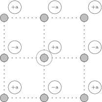
Since the minimisation of $\chi_{\epsilon}^{2}$ can lead to a potential that reconstructs the noise in the data, the solution needs to be regularised. Even without measurement errors, the intrinsic ellipticities would still produce pronounced small-scale noise peaks in the final reconstruction. In addition, the method presented here has an intrinsic invariance if no multiple imaging information is used and the weak lensing approximation $g\simeq\gamma$ applies. Namely, we can alternately add/subtract a constant $a$ along diagonals of the potential (chess-board like structure, as sketched in Fig. 3). This transformation would on the one hand not affect $\gamma$, but on the other it would cause a similar change (with a constant $2a/3$) in $\kappa$ – compare with Fig. 2. Thus in the $\left|g\right|\ll 1$ regime, where $\left\langle\epsilon\right\rangle=g\simeq\gamma$ these stripes would show up in the resulting $\kappa$-map. This problem can, however, be very efficiently cured with regularisation.

Figure 3: The intrinsic invariance of the method. If we alternately add/subtract a constant $a$ along the diagonals the shear $\gamma$ does not change (cf. Fig. 2), but $\kappa$ changes in the similar way with a constant now being $2a/3$ .

Since we want to measure the cluster mass, the regularisation should not influence breaking the mass-sheet degeneracy. For example, one of the possibilities considered by Seitz et al. (1998) for regularisation function was $R=\sum_{i,j=1}^{N_{\mathrm{x}},N_{\mathrm{y}}}\left|\nabla\kappa\right|^{2}$. However, as the authors mentioned, such regularisation would tend to flatten the profile and therefore affect the mass-sheet degeneracy breaking. Their maximum-entropy regularisation with moving prior (i.e. the prior in the regularisation is not kept constant, but adapted in the process of minimisation) does not flatten the profile, however it is very cumbersome to express its derivative in linear terms of $\psi_{k}$. Motivated by the success of moving prior in maximum-entropy regularisation, we choose a very simple prescription for the regularisation function. We start off by a relatively coarse grid, since if the number of grid points $N_{\rm dim}$ is much smaller than the number of galaxies, the resulting reconstruction is not able to follow the noise pattern. In each second-level iteration step we gradually increase the number of grid points and compare the resulting $\kappa$ map $\kappa^{(n_{2})}$ with that from the previous iteration $\kappa^{(n_{2}-1)}$ linearly interpolated on a finer grid, thus

$$R=\sum_{i,j=1}^{N_{\mathrm{x}},N_{\mathrm{y}}}\left(\kappa_{ij}^{(n_{2})}-\kappa_{ij}^{(n_{2}-1)}\right)^{2}\;.$$ (16)

For the case of $n_{2}=0$ we use an initial guess for $\kappa$ which can in practice be obtained from strong lensing, direct finite-field reconstruction, parametrised model fitting to weak lensing data, or simply set to $\kappa_{ij}^{(0)}=0$. This form of regularisation is relatively easy to implement and is in addition very efficient in removing the stripes (mentioned above) in the final reconstruction. If enough $n_{2}$ iteration steps are used this form of regularisation also does not substantially affect the ability to break the mass-sheet degeneracy, since the information of initial $\kappa^{(0)}$ is lost and different initial conditions do not bias the results (if the signal from lensing is high enough).

Finally a word on the regularisation constant $\eta$. This parameter should, in theory, be set such to ensure $\chi^{2}/N_{\rm dof}\sim 1$. In practice, however, it is difficult to determine its optimal value (in the critical lensing regime). As outlined in Geiger & Schneider (1998) the probability distribution of measured ellipticities is not a Gaussian and therefore the minimum value of $\chi^{2}$ has no particular meaning. In practice, setting $\eta$ such that the resulting $\chi^{2}/N_{\rm dof}\sim 1$ (where $N_{\rm dof}$ is in our case the number of galaxies used for strong and weak lensing) is valid is a good guess for this parameter. In addition, one adjusts $\eta$ low enough for the method to have enough freedom to adapt to the information in the data and large enough for not allowing the solutions that follow the noise pattern. As a rule of thumb it is usually better to set $\eta$ high and increase the number of iterations and hence allowing $\kappa$ to change only slowly. Since the reconstruction is done in a two-level iteration and in addition multiple-image information is included, the method can successfully adapt to the data and the results are not very sensitive to the precise value of $\eta$. The resulting smoothness level of the mass maps should reflect the quality of data. The “smoothing scale” depends upon the combination of the grid size and regularisation. The final potential map should be void of any structures on scales smaller than the mean separation between galaxies used for weak lensing. We will shortly return to this point in Sect. 4.3.

3.4 Initial conditions

For the purpose of the regularisation, given by (16), we need to employ the initial conditions. In addition, if a realistic model is used for the initial conditions (and as trial solution), it is very helpful to break the internal degeneracy, i.e. to distinguish galaxies that have $\left|g\right|\leq 1$ from those with $\left|g\right|>1$ in the first step, and thus allow for a faster convergence. Breaking this degeneracy is desirable, since otherwise the method has difficulties in “climbing” over the $\left|g\right|=1$ region (especially if no multiple-image systems are included). Since we use individual redshifts of background galaxies we do not have well-defined critical curves (i.e. positions in the source plane where $\left|g\right|=1$), as their position depends on the source redshift. In spite of this fact, the transition still poses a difficulty.

In our case different initial conditions are employed. For the initial model $\kappa^{(0)}$ we use three different scenarios: $\kappa^{(0)}=0$ (and $\@vec{\alpha}^{(0)}=\@vec{0}$, $\gamma^{(0)}=0$) across the whole field (hereafter I0), $\kappa^{(0)}$ taken from the best fit non-singular isothermal ellipsoid model NIE for the multiple image system described in Sect. 4.2 (hereafter IM) and a non-singular isothermal sphere model NIS with scaling and core radius being the same as in IM (hereafter IC). The same models are used also to obtain the initial coefficients of the linear system (see Appendix) (for I0 we use $\gamma_{1,2}=0$). These different initial models help us to explore the effects of regularisation and the capability of the reconstruction method to adapt to the data.

4 Cluster mass reconstruction from simulated data

4.1 Mock catalogues

(a)

(b)

Figure 4: The gravitational lensing properties of a simulated cluster used for generating mock catalogues for statistical weak lensing and for the multiple image system. a) The surface mass density $\kappa$, b) the absolute value of the reduced shear $\left|g\right|$, both for a source at $z_{\rm s}\to\infty$, are given in gray-scale and contours. The stars in a) denote the image positions of a four-image system at $z_{\rm s}=1.76$ which we use for the reconstruction.

We generate mock catalogues using a cluster from the high-resolution N-body simulation by Springel et al. (2001). The cluster is taken from the S4 simulation (for details see the aforementioned paper) and was simulated in the framework of the $\Lambda$CDM cosmology with density parameters $\Omega_{\rm m}=0.3$ and $\Omega_{\Lambda}=0.7$, shape parameter $\Gamma=0.21$, the normalisation of the power spectrum $\sigma_{8}=0.9$, and Hubble constant $H_{0}=70\;{\rm km\>s^{-1}\>Mpc^{-1}}$. The cluster simulation consists of almost 20 million particles, each with a mass of $4.68\times 10^{7}\;M_{\odot}$ and a gravitational softening length of $0.7\>h^{-1}\>{\rm kpc}$. Due to the high mass resolution, the surface mass density $\kappa$-map can be obtained by directly projecting the particles (in our case along the $z$-axis) onto a $1024^{2}$ grid (of a side length $4\mbox{ Mpc}$) using the NGP (nearest gridpoint) assignment.

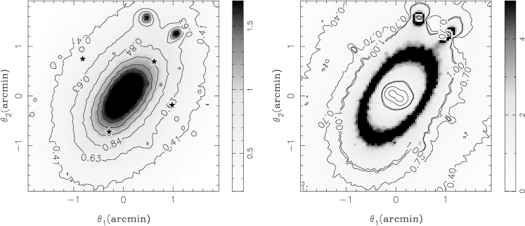
In what follows we try to generate the weak and strong lensing data to resemble as close as possible the data on the cluster RX J1347.5$-$1145 we will use in Paper II. The surface mass density of the cluster is therefore scaled to have a sizeable region where multiple imaging is possible within a $3.8\times 3.8\mbox{ arcmin}^{2}$ field, for sources at redshifts $z\gtrsim 1$ and a cluster at $z_{\rm d}=0.4$. The Einstein radius for a fiducial source at $z\to\infty$ is roughly $\theta_{\rm E}\sim 1^{\prime}$, giving a line-of-sight integrated mass within this radius of $\sim 5\times 10^{14}M_{\odot}$. The cut-out of the resulting $\kappa$ map (for $z\to\infty$, thus $Z(z)=1$) we use can be seen in Fig. 4a.

The lensing properties are calculated as described in detail in Bradač et al. (2004c). The Poisson equation for the lens potential $\psi$ – c.f. Eq. (3) – is solved on the grid in Fourier space with a DFT (Discrete Fourier Transformation) method using the FFTW library written by Frigo & Johnson (1998). The two components of the shear $\gamma_{1,2}$ and the deflection angle $\@vec{\alpha}$ are obtained by finite differencing methods applied to the potential $\psi$. These data are then used to generate the weak lensing catalogues as well as the multiple image systems. The absolute value of the reduced shear (again for a source with $z\to\infty$) is shown in Fig. 4b.

The weak lensing data are obtained by placing $N_{\rm g}$ galaxies on a $3.8\times 3.8\mbox{ arcmin}^{2}$ field. We have simulated two different catalogues, one with $N_{\rm g}=148$ galaxies with positions corresponding to those from R-band weak lensing data of the cluster RX J1347.5$-$1145 and one with $N_{\rm g}=210$ galaxies corresponding to the I-band data used in Paper II. In this way we simulate the effects of “holes”, resulting from cluster obscuration and bright stars in the field.

The intrinsic ellipticities $\epsilon_{\rm s}$ are drawn from a Gaussian distribution, each component is characterised by $\sigma=\sigma_{\epsilon^{\mathrm{s}}}=0.2$. We use the same redshifts as those measured in the R and I-band data, respectively. The catalogues have average redshifts for background sources of $\left\langle z_{\rm I}\right\rangle=1.18$ and $\left\langle z_{\rm R}\right\rangle=1.14$. The corresponding cosmological weights are evaluated assuming the $\Lambda$CDM cosmology (the same parameters are used as for the cluster simulations).

The measurement errors $\epsilon^{\rm err}$ on the observed ellipticities are drawn from a Gaussian distribution with $\sigma=\sigma_{\mathrm{err}}=0.1$ (each component) and added to the lensed ellipticities. We considered also the measurement errors on the redshifts of the galaxies to simulate the use of photometric redshifts. These have $\sigma_{\mathrm{zerr}}=0.1\left(1+z_{i}\right)$ (see Bolzonella et al. 2000); in adding the errors we ensured that the resulting redshifts are always positive. We have also simulated the presence of outliers in the redshift distribution, $10\%$ of our background sources (chosen at random) are considered outliers, for these we randomly add/subtract $\Delta z=1$ to their redshifts (which already include random errors). The lensed ellipticities are obtained using (9) and interpolating the quantities $\kappa$, and $\gamma$ at the galaxy position using bilinear interpolation, considering the redshifts including errors. In contrast, for the purpose of reconstruction we then consider galaxies to be at their ”original” redshifts (thus equal to the observed redshifts in the data of RX J1347.5$-$1145).

4.2 Multiple imaging

To obtain a four-image system from the simulation we use the method described in detail in Bradač et al. (2004c). With the MNEWT routine from Press et al. (1992) we solve the lens equation for a given source position inside the asteroid caustic. The source is assumed at a redshift of $z_{\rm s}=1.76$. Once we have the image positions, their magnifications are calculated and the fifth image is eliminated, since it is usually too dim and would not be observable.

The errors on image positions can be conservatively estimated (for the data we use in Paper II) to $\sim 0.\!\!^{\prime\prime}3$. Since we need errors in the source plane, we set them by a factor of five smaller (in agreement with the average magnification factor for this system), i.e. $\sigma_{{\rm s},m}=0.\!\!^{\prime\prime}06$ for both coordinates (see discussion in Sect. 3.3).

We also use this system to obtain one of the $\kappa^{(0)}$ models, needed for the purpose of strong and weak lensing reconstruction. We perform image plane minimisation and fit an NIE model (Kormann et al. 1994), given by

$$\kappa(\@vec{\theta}^{\prime})=\frac{b_{0}}{2\sqrt{\frac{1+\left|\epsilon_{\rm g}\right|}{1-\left|\epsilon_{\rm g}\right|}\left(r_{\rm c,nis}^{2}+(\theta^{\prime}_{1})^{2}\right)+(\theta^{\prime}_{2})^{2}}}\;,$$ (17)

where $\theta^{\prime}$ is calculated w.r.t. the semi-major axis of the cluster surface mass density. We allow the scaling $b_{0}$, ellipticity $\left|\epsilon_{\rm g}\right|$ and position angle $\phi_{g}$ to vary. The best fit model for this system has values of $\{b_{0},\left|\epsilon_{\rm g}\right|,\phi_{g}\}=\{0.\!\!^{\prime}97,0.30,1.01\}$. We fix the core radius $r_{\rm c}$ to $0.\!\!^{\prime}1$. For model fitting we use C-minuit (James & Roos 1975), a routine which is part of the CERN Program Library.

(a1)

(b1)

(c1)

(a2)

(b2)

(c2)

Figure 5: $\kappa$-maps obtained from combined strong and weak lensing reconstruction of the simulated data. Left panels show the reconstructions using $N_{\rm g}=210$ galaxies distributed in the same manner as the I-band, while for the right panels we use $N_{\rm g}=148$ galaxies distributed in the same manner as the R-band weak lensing data for RX J1347.5$-$1145 (see Paper II). The galaxies have been lensed by an N-body simulated cluster. Different initial conditions are used for the reconstruction. In a1-a2) we use best fit model from the multiple image system IM (see Sect. 4.2) in b1-b2) we use the IC model, an NIS model with the same scaling and core radius as IM and in c1-c2) we use I0, i.e. $\kappa^{(0)}=0$ on all grid points. The positions of the cluster centre and two major subclumps are plotted as white circles.

4.3 Weak lensing mass-reconstruction using simulated data

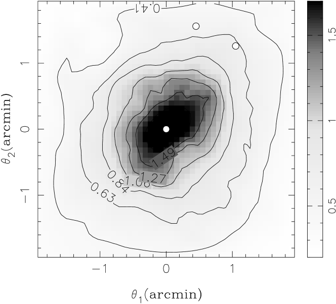
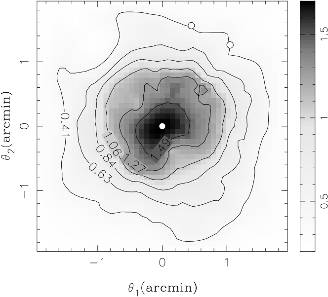
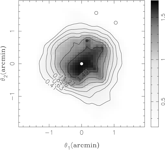
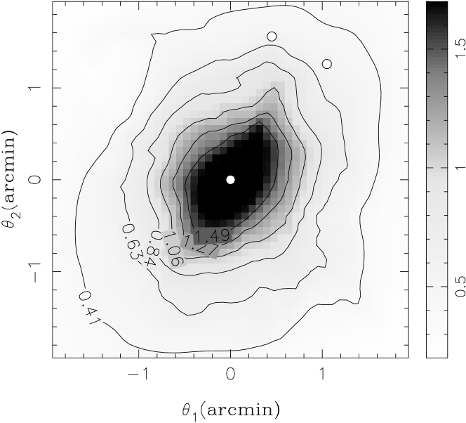
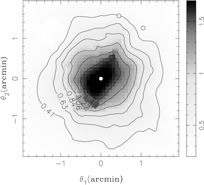
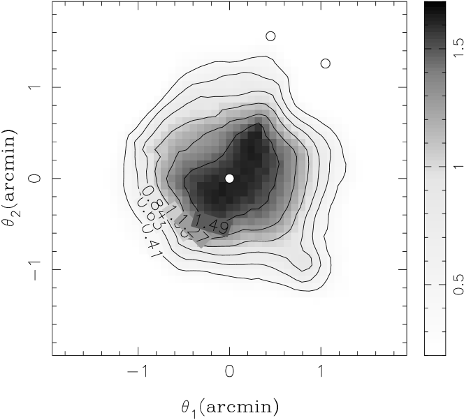
The mock catalogues are used to test the performance of the reconstruction method. We obtain the solution of the linear system with the UMFPACK routine for solving asymmetric sparse linear systems (Davis & Duff 1999). We perform 30 second-level iterations, each time increasing $N_{\mathrm{x}}$ and $N_{\mathrm{y}}$ by one, starting with an initial $20\times 20$ grid (since we use regularisation from the first iteration, we do not need to start the reconstruction with a very course grid, where the resulting matrix is not sparse and a different routine should be applied to find a good solution). The results of the reconstructions are shown in Fig. 5 for $N_{\rm g}=210$ galaxies distributed in the same manner as the I-band data and $N_{\rm g}=148$ galaxies distributed as the R-band data of the cluster described in Paper II. The initial regularisation parameter was set to $\eta=400$ for I-band $\eta=200$ for R-band data and adapted in each step to ensure $\chi^{2}/N_{\rm dof}\sim 1$. Two different initial values for the regularisation parameter are used since the numbers of galaxies in the two bands are different. It is very comforting to observe that the reconstructed maps do not depend crucially on the initial $\kappa$-model we use.

From the reconstructed maps we estimate the mass within the $1.\!\!^{\prime}5$ radius from the centre of the cluster (for a redshift $z_{\rm d}=0.4$ this corresponds to $340{h^{-1}}\mbox{ kpc}$) projected along the line-of-sight. For this purpose we generate 10 mock catalogues for each band and did the reconstruction again with the three different initial models. We list the resulting average mass obtained from the catalogues in Table 1 for both the I- and R-band mock catalogues. All the mass estimates are similar; note, however, that the galaxy catalogues following the I- and R-band data have galaxies partly in common and the errors are therefore correlated. We find the enclosed mass of the simulated cluster to be $(1.0\pm 0.1)\times 10^{15}M_{\odot}$, which is very close to the input value of $M_{\rm s}(<340{h^{-1}}\mbox{ kpc})=0.99\times 10^{15}M_{\odot}$. The 1-$\sigma$ error is estimated from the variance of mass determinations from different mock catalogues.

The results show that our method is effectively able to break the mass-sheet degeneracy and is, as a consequence, very efficient in reproducing the cluster mass also at radii significantly larger than the Einstein radius of the cluster. It is also very encouraging that the results are nearly independent of the initial $\kappa^{(0)}$ used for the regularisation. Note that a single multiple-image system does not by itself break this degeneracy, we would need at least two different redshift multiple image systems to break the mass-sheet degeneracy with strong lensing data alone. In such a case the strong lensing gives constraints on the mass enclosed within the Einstein radius for a given source redshift and since the critical curves depend on the source redshift, we can constrain mass at two different radii and the degeneracy is broken. The combiniation of weak and strong lensing is the more powerful, the more different the redshift of the source of the multiple images is from the median redshift of the galaxies from which the weak lensing measurements are obtained, and the less symmetric the arrangement of multiple images is w.r.t. the center of the cluster.

Unfortunately we can not resolve both clumps present in the simulations. This is due to the fact that the number density of background sources is low and the internal smoothing scale (i.e. the average distance between two source galaxies) is large; with a number density of $\sim 100\mbox{ arcmin}^{-2}$ the clumps can be easily resolved.

We have also performed additional reconstructions in which we multiplied the original values of $\kappa$ of the simulated cluster by $0.75$ and $1.25$. This enables us to confirm that the agreement between input mass and reconstructed mass is not just accidental. We have generated new multiple image systems and new mock catalogues as before. We do not, however, perform a new strong-lensing reconstruction, for $\kappa^{(0)}$ we intentionally use the same (i.e. in this case “wrong”) initial conditions as before. The old IM model would not fit the image positions any longer, since they have changed with the scaling of $\kappa$. The reconstructed masses of the increased $\kappa$ simulation are in good agreement with the input values. The differences between different models are comparable (slightly smaller) to the ones shown in Table 1. For the lower $\kappa$ simulation, the reconstructed values are on average the same as the input value, however the scatter is larger. This is expected, since the lens in this case is weaker and the breaking of the mass-sheet degeneracy is difficult in this case (with the quality of data used here).

As an additional test we also consider a redshift distribution with $\left\langle z\right\rangle=1.6$ for the sources used for weak lensing and regenerate the mock catalogues. The accuracy of the determination of the enclosed mass increases. However, more importantly, we also better reconstruct the shape of the mass distribution, since high-redshift galaxies (when their shape is measured reliably) contribute most to the signal and improve the accuracy of the reconstruction.

Table 1: Reconstructed cluster mass within a cylinder of $340{h^{-1}}\mbox{ kpc}$ radius around the cluster centre from simulations of mock catalogues resembling I-band (left) and R-band (right) weak lensing data and one 4-image system. Three different initial conditions are used. We use the best fit model from the multiple image system IM (see Sect. 4.2), the IC model (NIS with same scaling and core radius as IM) and I0 with $\kappa^{(0)}=0$ on all grid points. In the last line the input mass $M_{\rm s}$ from the simulation is given. The variance of the mass estimate is given and in brackets we give for comparison the velocity dispersion of an SIS having the same enclosed mass within $340{h^{-1}}\mbox{ kpc}$.

	$M_{I,\rm s}$	$[\sigma_{\rm I,SIS}]$	$M_{R,\rm s}$	$[\sigma_{\rm R,SIS}]$
	$[10^{15}M_{\odot}]$	$[{\rm kms^{-1}}]$	$[10^{15}M_{\odot}]$	$[{\rm kms^{-1}}]$
IM	$1.07\pm 0.02$	[1720]	$1.04\pm 0.02$	[1710]
IC	$1.04\pm 0.02$	[1700]	$1.00\pm 0.02$	[1670]
I0	$0.88\pm 0.03$	[1560]	$0.82\pm 0.03$	[1510]
$M_{\rm s}(<340{h^{-1}}\mbox{ kpc})$			0.99	[1670]

5 Conclusions

In this paper we develop a new method based on Bartelmann et al. (1996) to perform a combined weak and strong lensing cluster mass reconstruction. The particular strength of this method is that we extend the weak lensing analysis to the critical parts of the cluster. In turn, this enables us to directly include multiple imaging information to the reconstruction. Strong and weak lensing reconstructions are performed on the same scales, in contrast to similar methods proposed in the past where weak lensing information on much larger radii than the Einstein radius $\theta_{\rm E}$ was combined with strong lensing information (see e.g. Kneib et al. 2003).

We test the performance of the method on simulated data and conclude that if a quadruply imaged system combined with weak lensing data and individual photometric redshifts is used, the method can very successfully reconstruct the cluster mass distribution. With a relatively low number density of background galaxies, $15\mbox{ arcmin}^{-2}$, we are effectively able to reproduce the main properties of the simulated cluster. In addition, with larger number densities $\sim 100\mbox{ arcmin}^{-2}$ of background sources, accessible by HST, the substructures in the cluster can be resolved and the mass determination further improved.

We determine the enclosed mass within $340{h^{-1}}\mbox{ kpc}$ of the simulated cluster to be $(1.0\pm 0.1)\times 10^{15}M_{\odot}$, which is very close to the input value of $M_{\rm s}(<340{h^{-1}}\mbox{ kpc})=0.99\times 10^{15}M_{\odot}$. We have shown, that with the data quality we use we are effectively able to break the mass-sheet degeneracy and therefore obtain the mass and mass-distribution estimates without prior assumptions on the lensing potential.

In addition, the reconstruction algorithm can be improved in many ways. First, we use for the multiply imaged system only the information of the image positions. The reconstruction method can, however, be modified to include the morphological information of each extended source. Instead of using a regular grid, one would have to use adaptive grids and decrease the cell sizes around each of these images. This will be a subject of a future work. Second, the photometric redshift determination does not only give the most likely redshift given the magnitudes in different filters, but also the probability distribution for the redshift. This information can be included in the reconstruction. In addition, source galaxies without redshift information can be included and different regularisation schemes can be considered.

Finally, the slight dependence on the initial conditions is getting weaker the higher the number density of background galaxies and/or multiple image systems are. In addition, it is of advantage to have a large spread in the redshift efficiency factors $Z$ of the background galaxies. For example, deep ACS images of clusters with a usable number density of $n\sim 120\mbox{ arcmin}^{-2}$, or future observations with the James Webb Space Telescope will most likely make the dependence on the initial conditions negligible.

In Paper II we will show the application of this method on the cluster RX J1347.5$-$1145 and confirm that a combination of strong and weak lensing offers a unique tool to pin down the masses of galaxy-clusters as well as their mass distributions.

Appendix A The linear problem for $\psi_{k}$

In this section we present details of the method outlined in Sect. 3.

We aim to solve the equation

$$\frac{\partial\chi_{\epsilon}^{2}(\psi_{k})}{\partial\psi_{k}}+\frac{\partial\chi_{\rm M}^{2}(\psi_{k})}{\partial\psi_{k}}+\eta\frac{\partial R(\psi_{k})}{\partial\psi_{k}}=0\;.$$ (18)

This is in general a non-linear system of equations. We try to solve it in an iterative way by linearising the equation in terms of $\psi_{k}$ and keeping the non-linear terms fixed at each iteration step. The resulting system is then written in the form

$$\mathcal{B}_{jk}\psi_{k}=V_{j}\;,$$ (19)

where the matrix $\mathcal{B}_{jk}$ and vector $V_{j}$ contain the contributions from the non-linear part. In the following sections we will describe the contributions to (18) in turn.

A.1 The weak lensing analysis

The $\chi_{\epsilon}^{2}$ for the weak lensing case is given in (13). From now on we consider in detail only the $\left|g\right|\leq 1$ case; for $\left|g\right|>1$, the calculations are done in the same fashion. First we plug into (13) the expectation value of observed ellipticities (i.e. the reduced shear $g$) obtaining

$$\chi_{\epsilon}^{2}(\psi_{k})=\sum_{i=1}^{N_{\mathrm{g}}}\frac{\left|\epsilon-\frac{Z\gamma}{1-Z\kappa}\right|^{2}}{\sigma^{2}}=\sum_{i=1}^{N_{\mathrm{g}}}\frac{\left|\epsilon-Z\epsilon\kappa-Z\gamma\right|^{2}}{\left(1-Z\kappa\right)^{2}\sigma^{2}}\;,$$ (20)

where $\kappa$, $\gamma$, and $\sigma$ depend on $\@vec{\theta}_{i}$ only and $Z$ depends on the redshift of the $i$-th source. Note that for simplicity we omit the index $i$ to $\epsilon$, $\kappa$, $\gamma$, $\sigma$ and $Z$, although these quantities are different for every galaxy. As described in Sect. 3.2 using finite differencing and bilinear interpolation, we can write $\kappa$ and $\gamma$ at each galaxy position as a linear combination of $\psi_{k}$. This is expressed in the following matrix notation

$$\gamma_{1}(\@vec{\theta}_{i})=\mathcal{G}^{(1)}_{ik}\psi_{k}\;,\;\;\;\gamma_{2}(\@vec{\theta}_{i})=\mathcal{G}^{(2)}_{ik}\psi_{k}\;,\;\;\;\kappa(\@vec{\theta}_{i})=\mathcal{K}_{ik}\psi_{k}\;,$$ (21)

where the matrices $\mathcal{G}^{(1)}_{ik}$, $\mathcal{G}^{(2)}_{ik}$, and $\mathcal{K}_{ik}$ are composed of numerical factors described in Sect. 3.2. Now we consider the denominator of (20) $\hat{\sigma}_{\leq}^{2}=\left(1-Z\kappa\right)^{2}\sigma^{2}$ fixed at each iteration step (the subscript $\leq$ denotes the $\left|g\right|\leq 1$ case) and differentiate the following term of (20)

$$\;\frac{1}{2}\frac{\partial}{\partial\psi_{k}}\frac{\left|\epsilon-Z\epsilon\kappa-Z\gamma\right|^{2}}{\hat{\sigma}_{\leq}^{2}}=$$ (22)

$$-\;\frac{Z}{\hat{\sigma}_{\leq}^{2}}\left[\left(\epsilon_{1}-Z\epsilon_{1}\kappa-Z\gamma_{1}\right)\left(\epsilon_{1}\frac{\partial\kappa}{\partial\psi_{k}}+\frac{\partial\gamma_{1}}{\partial\psi_{k}}\right)\right.$$

$$+\;\left.\left(\epsilon_{2}-Z\epsilon_{2}\kappa-Z\gamma_{2}\right)\left(\epsilon_{2}\frac{\partial\kappa}{\partial\psi_{k}}+\frac{\partial\gamma_{2}}{\partial\psi_{k}}\right)\right]=$$

$$\phantom{-}\;\;\frac{Z^{2}}{\hat{\sigma}_{\leq}^{2}}\Big{[}\mathcal{G}^{(1)}_{ij}\mathcal{G}^{(1)}_{ik}+\mathcal{G}^{(2)}_{ij}\mathcal{G}^{(2)}_{ik}+\epsilon_{1}\left(\mathcal{G}^{(1)}_{ij}\mathcal{K}_{ik}+\mathcal{K}_{ij}\mathcal{G}^{(1)}_{ik}\right)$$

$$+\;\;\epsilon_{2}\left(\mathcal{G}^{(2)}_{ij}\mathcal{K}_{ik}+\mathcal{K}_{ij}\mathcal{G}^{(2)}_{ik}\right)+\left(\epsilon_{1}^{2}+\epsilon_{2}^{2}\right)\mathcal{K}_{ij}\mathcal{K}_{ik}\Big{]}\psi_{k}$$

$$-\;\;\frac{Z^{2}}{\hat{\sigma}_{\leq}^{2}}\left[\epsilon_{1}\mathcal{G}^{(1)}_{ij}+\epsilon_{2}\mathcal{G}^{(2)}_{ij}+\left(\epsilon_{1}^{2}+\epsilon_{2}^{2}\right)\mathcal{K}_{ij}\right]$$

where $\epsilon_{1}$ and $\epsilon_{2}$ are the two components of the measured ellipticity of galaxy $i$ (again omitting the index and we divided Eq. (18) by two for simplicity). We sum over all galaxies used for the weak lensing analysis and obtain a linear problem for $\psi_{k}$ at each iteration step. The same approach can be used for the $\left|g\right|>1$ case, where $\hat{\sigma}_{>}^{2}$ is kept constant and is given by $\hat{\sigma}_{>}^{2}=Z_{i}^{2}\left|\gamma\right|^{2}\sigma_{i}^{2}$.

A.2 The strong-lensing term

Following the prescription from the previous section we now write the deflection angle in a matrix form

$$\alpha_{1}(\@vec{\theta}_{m})=\mathcal{D}^{(1)}_{ik}\psi_{k}\;,\;\;\;\alpha_{2}(\@vec{\theta}_{m})=\mathcal{D}^{(2)}_{ik}\psi_{k}\;.$$ (23)

Both matrices give the finite differencing form for the gradient of the potential, in particular we use the central differencing formula, i.e. $\alpha_{1}(0,0)=\frac{1}{2\Delta}\left(\psi(1,0)-\psi(-1,0)\right)$ and $\alpha_{2}(0,0)=\frac{1}{2\Delta}\left(\psi(0,1)-\psi(0,-1)\right)$.

The $\chi^{2}$ contribution to strong lensing is given in (15). The source position $\@vec{\beta}_{\rm s}$ is kept constant at every iteration step, and is evaluated using the deflection angle information $\@vec{\alpha}^{(n_{1}-1)}$ from the previous iteration

$$\@vec{\beta}_{\rm s}=\frac{1}{N_{\rm M}}\sum_{m=1}^{N_{\rm M}}\left(\@vec{\theta}_{\rm m}-Z(z_{\rm s})\@vec{\alpha}^{(n_{1}-1)}(\@vec{\theta}_{m})\right)\;.$$ (24)

We differentiate the following term in $\chi^{2}_{\rm M}$ (for the $x_{1}$-coordinate)

$$\frac{1}{2}\frac{\partial}{\partial\psi_{k}}\frac{\left(\theta_{\rm m,1}-Z(z_{\rm s})\alpha_{1}(\@vec{\theta}_{m})-\beta_{\rm s,1}\right)^{2}}{\sigma_{{\rm s},m(1)}^{2}}=$$ (25)

$$-\frac{\left(\theta_{m,1}-\beta_{\rm s,1}\right)\mathcal{D}^{(1)}_{ij}-Z(z_{\rm s})\mathcal{D}^{(1)}_{ij}\mathcal{D}^{(1)}_{ik}\psi_{k}}{\sigma_{{\rm s},m(1)}^{2}}\;.$$

The expression for the $x_{2}$-coordinate is obtained by exchanging $1\rightarrow 2$. After summation of both terms over all images $m$ we get a set of equations which are linear in $\psi_{k}$ and can be readily included in (19). In principle we could also use $\@vec{\alpha}(\psi_{k})$ in (24), the expression $\partial\chi_{\rm M}^{2}/\partial\psi_{k}$ would remain linear in $\psi_{k}$. However since the first approach is computationally much simpler, we use the former.

A.3 The final result

In the previous section we describe how we linearise the contributions of weak and strong lensing, now we can write the coefficients in the equation (19). Note that the contribution of the regularisation term (with $\chi^{2}$-contribution given in (16)) is already linear in $\psi_{k}$ and therefore the full matrix $\mathcal{B}_{jk}$ is given in the form

$$\mathcal{B}_{jk} = \sum_{i=1}^{N_{\rm gal}}\left[a_{11}(i)\mathcal{G}^{(1)}_{ij}\mathcal{G}^{(1)}_{ik}+a_{22}(i)\mathcal{G}^{(2)}_{ij}\mathcal{G}^{(2)}_{ik}\right.$$ (26)

$$\qquad+a_{13}(i)\left(\mathcal{G}^{(1)}_{ij}\mathcal{K}_{ik}+\mathcal{G}^{(1)}_{ik}\mathcal{K}_{ij}\right)$$

$$\qquad+a_{23}(i)\left(\mathcal{G}^{(2)}_{ij}\mathcal{K}_{ik}+\mathcal{G}^{(2)}_{ik}\mathcal{K}_{ij}\right)$$

$$\qquad\left.+a_{33}(i)\left(\mathcal{K}_{ij}\mathcal{K}_{ik}\right)\right]$$

$$+ \sum_{m=1}^{N_{\rm M}}b_{11}(m)\mathcal{D}^{(1)}_{mj}\mathcal{D}^{(1)}_{mk}+b_{22}(m)\mathcal{D}^{(2)}_{mj}\mathcal{D}^{(2)}_{mk}$$

$$+ \eta\sum_{g}\mathcal{K}_{gj}\mathcal{K}_{gk}\;,$$

where the sums over $i$, $g$ and $m$ denote summation over all galaxies with ellipticity measurements, all grid points, and all images in the multiple imaged system, respectively. The $V_{j}$ vector carries the information of all constant terms in (18)

$$V_{j} = \sum_{i=1}^{N_{\rm gal}}a_{1}(i)\mathcal{G}^{(1)}_{ij}+a_{2}(i)\;\mathcal{G}^{(2)}_{ij}+a_{3}(i)\;\mathcal{K}_{ij}$$ (27)

$$+ \eta\sum_{g}\kappa^{(n_{2}-1)}\mathcal{K}_{gj}$$

$$+ \sum_{m=1}^{N_{\rm M}}b_{1}(m)\mathcal{D}^{(1)}_{mj}+b_{2}(m)\;\mathcal{D}^{(2)}_{mj}\;.$$

The coefficients $a$ now differ depending on whether we are in the $\left|g\right|\leq 1$ or $\left|g\right|>1$ regime. For $\left|g\right|\leq 1$ the coefficients are given by

$$a_{11}(i) = a_{22}(i)=\frac{Z^{2}}{\hat{\sigma}_{\leq}^{2}}\;;\;\;\;a_{13}(i)=\frac{Z^{2}}{\hat{\sigma}_{\leq}^{2}}\epsilon_{1}\;;$$

$$a_{23}(i) = \frac{Z^{2}}{\hat{\sigma}_{\leq}^{2}}\epsilon_{2}\;;\;\;\;a_{33}(i)=\frac{Z^{2}}{\hat{\sigma}_{\leq}^{2}}\left|\epsilon\right|^{2}\;;$$

$$a_{1}(i) = \frac{Z}{\hat{\sigma}_{\leq}^{2}}\epsilon_{1}\;;\;a_{2}(i)=\frac{Z}{\hat{\sigma}_{\leq}^{2}}\epsilon_{2}\;;\;a_{3}(i)=\frac{Z}{\hat{\sigma}_{\leq}^{2}}\left|\epsilon\right|^{2}\;.$$ (28)

For $\left|g\right|>1$ case we get

$$a_{11}(i) = a_{22}(i)=\frac{Z^{2}}{\hat{\sigma}_{>}^{2}}\left|\epsilon\right|^{2}\;;\;\;\;a_{13}(i)=\frac{Z^{2}}{\hat{\sigma}_{>}^{2}}\epsilon_{1}\;;$$

$$a_{23}(i) = \frac{Z^{2}}{\hat{\sigma}_{>}^{2}}\epsilon_{2}\;;\;\;\;a_{33}(i)=\frac{Z^{2}}{\hat{\sigma}_{>}^{2}}\;;$$

$$a_{1}(i) = \frac{Z}{\hat{\sigma}_{>}^{2}}\epsilon_{1}\;;\;a_{2}(i)=\frac{Z}{\hat{\sigma}_{>}^{2}}\epsilon_{2}\;;\;a_{3}(i)=\frac{Z}{\hat{\sigma}_{>}^{2}}\;.$$ (29)

The coefficients $b$ are carrying the information about the multiple imaged system:

$$b_{11}(m) = \frac{Z^{2}(z_{\rm s})}{\sigma_{{\rm s},m(1)}^{2}}\;;\;\;\;b_{22}(m)=\frac{Z^{2}(z_{\rm s})}{\sigma_{{\rm s},m(2)}^{2}}\;;$$

$$b_{1}(m) = \frac{Z(z_{\rm s})\left(\theta_{m,1}-\beta_{{\rm s},1}\right)}{\sigma_{{\rm s},m(1)}^{2}}\;;$$

$$b_{2}(m) = \frac{Z(z_{\rm s})\left(\theta_{m,2}-\beta_{{\rm s},2}\right)}{\sigma_{{\rm s},m(2)}^{2}}\;,$$ (30)

where $\theta_{m,1}$, $\theta_{m,2}$, and $\sigma_{{\rm s},m(1,2)}$ are defined in Sect. 3.3. For the reasons mentioned in Sect. 3.3 we consider the measurement errors projected to the source plane isotropic, we set $\sigma_{{\rm s},m(1,2)}$ equal for the purpose of the reconstruction.

References

- Abdelsalam et al. (1998) Abdelsalam, H. M., Saha, P., & Williams, L. L. R. 1998, AJ, 116, 1541
- Abramowitz & Stegun (1972) Abramowitz, M. & Stegun, I. A. 1972, Handbook of Mathematical Functions (Handbook of Mathematical Functions, New York: Dover, 1972)
- Allen (1998) Allen, S. W. 1998, MNRAS, 296, 392
- Bartelmann & Meneghetti (2004) Bartelmann, M. & Meneghetti, M. 2004, A&A, 418, 413
- Bartelmann et al. (1996) Bartelmann, M., Narayan, R., Seitz, S., & Schneider, P. 1996, ApJ, 464, L115
- Bartelmann & Schneider (2001) Bartelmann, M. & Schneider, P. 2001, Phys. Rep, 340, 291
- Bolzonella et al. (2000) Bolzonella, M., Miralles, J.-M., & Pelló, R. 2000, A&A, 363, 476
- Bradač et al. (2004a) Bradač, M., Erben, T., Schneider, P., et al. 2004a, astro-ph/0410642
- Bradač et al. (2004b) Bradač, M., Lombardi, M., & Schneider, P. 2004b, A&A, 424, 13
- Bradač et al. (2004c) Bradač, M., Schneider, P., Lombardi, M., et al. 2004c, A&A, 423, 797
- Broadhurst et al. (2005) Broadhurst, T., Takada, M., Umetsu, K., et al. 2005, ApJ, 619, L143
- Broadhurst et al. (1995) Broadhurst, T. J., Taylor, A. N., & Peacock, J. A. 1995, ApJ, 438, 49
- Clowe & Schneider (2001) Clowe, D. & Schneider, P. 2001, A&A, 379, 384
- Clowe & Schneider (2002) Clowe, D. & Schneider, P. 2002, A&A, 395, 385
- Dalal & Keeton (2003) Dalal, N. & Keeton, C. R. 2003, astro-ph/0312072
- Davis & Duff (1999) Davis, T. A. & Duff, I. S. 1999, ACM Trans. Math. Softw., 25, 1
- Diego et al. (2004) Diego, J. M., Protopapas, P., Sandvik, H. B., & Tegmark, M. 2004, astro-ph/0408418
- Ettori & Lombardi (2003) Ettori, S. & Lombardi, M. 2003, A&A, 398, L5
- Frigo & Johnson (1998) Frigo, M. & Johnson, S. 1998, in 1998 ICASSP conference proceedings, Vol. 3, 1381
- Gavazzi et al. (2004) Gavazzi, R., Mellier, Y., Fort, B., Cuillandre, J.-C., & Dantel-Fort, M. 2004, A&A, 422, 407
- Geiger & Schneider (1998) Geiger, B. & Schneider, P. 1998, MNRAS, 295, 497
- James & Roos (1975) James, F. & Roos, M. 1975, Computer Physics Communications, 10, 343
- Kaiser & Squires (1993) Kaiser, N. & Squires, G. 1993, ApJ, 404, 441
- Kneib et al. (2003) Kneib, J., Hudelot, P., Ellis, R. S., et al. 2003, ApJ, 598, 804
- Kochanek (2004) Kochanek, C. S. 2004, astro-ph/0407232
- Kormann et al. (1994) Kormann, R., Schneider, P., & Bartelmann, M. 1994, A&A, 284, 285
- Lombardi et al. (2005) Lombardi, M., Rosati, P., Blakeslee, J. P., et al. 2005, astro-ph/0501150
- Navarro et al. (1997) Navarro, J. F., Frenk, C. S., & White, S. D. M. 1997, ApJ, 490, 493
- Press et al. (1992) Press, W. H., Teukolsky, S. A., Vetterling, W. T., & Flannery, B. P. 1992, Numerical recipes in C. The art of scientific computing (Cambridge: University Press, 1992, 2nd ed.)
- Sand et al. (2004) Sand, D. J., Treu, T., Smith, G. P., & Ellis, R. S. 2004, ApJ, 604, 88
- Schneider et al. (2000) Schneider, P., King, L., & Erben, T. 2000, A&A, 353, 41
- Schneider & Seitz (1995) Schneider, P. & Seitz, C. 1995, A&A, 294, 411
- Seitz & Schneider (1997) Seitz, C. & Schneider, P. 1997, A&A, 318, 687
- Seitz et al. (1998) Seitz, S., Schneider, P., & Bartelmann, M. 1998, A&A, 337, 325
- Smith et al. (2004) Smith, G. P., Kneib, J., Smail, I., et al. 2004, astro-ph/0403588
- Springel et al. (2001) Springel, V., White, S. D. M., Tormen, G., & Kauffmann, G. 2001, MNRAS, 328, 726
- Tyson et al. (1990) Tyson, J. A., Wenk, R. A., & Valdes, F. 1990, ApJ, 349, L1