Multivariate Monte Carlo Methods for the Reflection Grating Spectrometers on XMM-Newton

Abstract

We propose a novel multivariate Monte Carlo method as an efficient and flexible approach to analyzing extended X-ray sources with the Reflection Grating Spectrometer (RGS) on XMM Newton. A multi-dimensional interpolation method is used to efficiently calculate the response function for the RGS in conjunction with an arbitrary spatially-varying spectral model. Several methods of event comparison that effectively compare the multivariate RGS data are discussed. The use of a multi-dimensional instrument Monte Carlo also creates many opportunities for the use of complex astrophysical Monte Carlo calculations in diffuse X-ray spectroscopy. The methods presented here could be generalized to other X-ray instruments as well.

1 The General Problem of Diffuse X-ray Spectroscopy

Diffuse sources, such as clusters of galaxies, supernova remnants, and the interstellar hot haloes of elliptical galaxies, comprise some of the most interesting targets for astrophysical X-ray spectroscopy. Photons from these sources are focused and dispersed by optics and recorded in detectors designed to measure three interesting quantities: two related to the position on the detector ($x$, $y$) and one related to an intrinsic photon energy measurement ($p$). These quantities are indirectly related to the sky coordinates ($\theta,\phi$) and the energy of the incident photon ($e$) that can be predicted from an astrophysical model with parameters, {$\eta_{1}$, $\eta_{2}$, $\eta_{3}$, …} $\equiv$ $\eta_{i}$.

The fundamental goal of data analysis for diffuse X-ray spectroscopy is to calculate the probability of a given distribution of photons in the ($x$, $y$, $p$) data-space given the parameters of a particular astrophysical model. Prior to the launch of the Chandra (Weisskopf et al. 2000) and XMM-Newton (Jansen et al. 2001) observatories, available instruments were characterized by sufficiently poor spatial and/or spectral resolution that simple one-dimensional spectral fitting techniques applied to data extracted from the image were sufficient for most applications. However, the grating experiments and non-dispersive CCD experiments on these two new observatories both have significant imaging and spectral capabilities, making it warranted to develop new techniques that utilize the full dimensionality of the data. In particular, the Reflection Grating Spectrometers (RGS) on XMM-Newton have a number of unique characteristics that make them powerful X-ray spectrometers for arcminute-size X-ray sources. In this paper, we demonstrate that the complex nature of the response function for the RGS requires new analysis methods that utilize the full dimensionality of the data. We also demonstrate how these methods might be useful for other X-ray instruments.

The techniques for analyzing an X-ray spectrum of an unresolved source are well-developed and have been essentially unchanged since the analysis of early X-ray spectra (Gorenstein, Gursky, & Garmire 1968). For that case, there is only one interesting measured quantity that is related to the energy of the photon. For non-dispersive spectrometers (e.g. CCDs, calorimeters, and proportional counters), the photon energy measurement ($p$) is the useful quantity. For dispersive spectrometers (e.g. gratings and crystals), the dispersion coordinate, $x$, or the position along the detector parallel to the dispersion axis, is the useful measured value. In either case, the detection probability, $D$, of finding a photon at a given $x$ or $p$ is then given by

$$D(x~{}\mbox{or}~{}p~{}|~{}\eta_{i})=\int de~{}R(x~{}\mbox{or}~{}p~{}|~{}e)~{}S(e~{}|~{}\eta_{i})$$ (1)

which is an integral over all energies, $e$. Here, R is the response kernel and S is the input spectral model, which is a function of both the energy and the input parameters. The response kernel describes the probability of obtaining a distribution of measured values given a photon with incident energy, $e$. The integral is computed numerically by converting the expression into a sum of discrete energies in well-developed software packages, such as XSPEC (Arnaud 1996) or SPEX (Kaastra et al. 1996).

For an extended source, the probability distribution is described by a three-dimensional function and its calculation requires an integration over both the sky coordinates ($\theta,~{}\phi$) and the intrinsic energy ($e$). The three-dimensional detection probability, D, is then given by

$$D(x,y,p~{}|~{}\eta_{i})=\int de~{}d\theta~{}d\phi~{}R(x,y,p~{}|~{}\theta,\phi,e)~{}S(\theta,\phi,e~{}|~{}\eta_{i})$$ (2)

Computing this entire integral directly is often impractical. Nevertheless, some approximations can be made that are useful in restricted situations. In particular, one can assume: 1) the source spectrum is independent of spatial position, and 2) the response does not vary as function of the off-axis angle. The problem can then be reduced to a one-dimensional integral, as for a point source. The former assumption is sometimes justified, but has become untenable in many recent analyses. For example, modeling an X-ray cluster of galaxies as a thermal plasma whose temperature varies spatially already violates this assumption. The second assumption depends on the nature of the X-ray instrument as well as the angular scale of the problem being investigated. Attempts to circumvent this problem by weighting the response matrix for Chandra ACIS-S observations can be found in Markevitch & Vikhlinin (2001) and in Arnaud et al. (2001) for XMM-Newton EPIC data. We demonstrate in §2 that the complex nature of the response function, $R$, for the Reflection Grating Spectrometer makes this approximation impossible to implement without assuming that there is no spectral variation over the entire field of view. Instead, we are forced to consider new methods that consider the full multi-dimensionality of Equation 2.

Equation 2 can be evaluated directly through a Monte Carlo calculation as we will demonstrate in §3. It has been known for some time that Monte Carlo methods are efficient for the evaluation of multi-dimensional integrals (Metropolis & Ulam 1949). Few photons are typically detected in X-ray observations, so the exact calculation of the full integral is superfluous. After constructing an efficient Monte Carlo algorithm, we outline a generic approach for the analysis of diffuse X-ray sources with Monte Carlo calculations in §4. In §5, we discuss several methods of event comparison that can be used with the photons simulated with the RGS Monte Carlo and real data. In §6, we discuss several straightforward extensions to these methods.

2 Structure of the RGS Response Function

The Reflection Grating Spectrometers consist of three instrumental components: the mirror module, the RGS grating array (RGA), and the RGS focal plane cameras (RFC). There are two nearly identical sets of each of the three components. The full description and calibration of these components has been covered in den Herder et al. (2001) and is also documented in the XMM Users Handbook. We briefly discuss some of the important characteristics of each of the three components for the purpose of data analysis.

The mirror module consists of 58 concentrically-aligned gold-coated mirrors shells. Photons hit each Wolter Type I shell twice. The angular resolution is set by surface deformations of the mirrors and the relative alignment of the shells. The X-rays then arrive at the reflection grating array (RGA) after exiting the mirror module. The RGA consists of 182 coaligned rectangular reflection gratings. Each grating has many triangular replicated grooves spaced at 645.6 lines per millimeter. On-axis X-rays hit the grating at 1.57 degrees and are dispersed between 2 and 5 degrees depending on their wavelength. The gratings are precisely arranged in an array, which is aligned so that all light hits the gratings at the same incidence angle (Kahn et al. 1996). If $\alpha$ is the angle of incidence of a photon, then the exit angle, $\beta$, is determined by the dispersion equation:

$$\frac{m\lambda}{d}=\cos{\beta}-\cos{\alpha}$$ (3)

where $d$ is the grating spacing and $m$ is the integer diffraction order. The derivation of this relation is straightforward through Fraunhofer diffraction theory. The deviation from this ideal relation is not simple, however, because it depends on the alignment of the array, the surface imperfections of the gratings, and the achromatic blurring already induced by the mirror module. The angle of incidence on the grating, $\alpha$, is related to the off-axis angle relative to the boresight axis, $\theta$, by

$$\theta=\frac{F}{L}\left(\alpha-\alpha_{0}\right)$$ (4)

where $F$ is the distance between the RGA and the RFC (6.7m) and $L$ is the focal length of the telescope (7.5m). For directions perpendicular to the grooves of the gratings, photons that enter at an angle, $\phi$, will exit at the same angle, which we will call cross-dispersion and designate by the angle, $y$. The cross-dispersion equation is then simply,

$$y=-\phi$$ (5)

The photons are detected by the RFC. Each RFC consists of 9 back-illuminated CCDs placed in a row that detect individual X-rays. Each CCD measures 1024 by 384 pixels, which are 27 microns on a side. Each CCD consists of two nodes where the charge is clocked separately for each. The intrinsic CCD energy resolution, which is set by the ability to fully sample the energy deposited in the charge cloud, is sufficient to separate the spectral orders for sets of photons. We would otherwise be left with an ambiguity between wavelength and spectral order. The gain-corrected pulseheight, $p$, is roughly proportional to the energy,

$$p=e$$ (6)

The CCD array is approximately aligned along the Roland circle in the RGS design so that the position along the detector array, $x$, is approximately equal to the exit angle for the grating, $\beta$, after correcting for the relative locations of the individual CCDs. For that reason, we will use $\beta$ and $x$ interchangeably.

The Reflection Grating Spectrometers were designed to have relatively high dispersion (i.e., large dispersion angles from the focus) in order to compensate for the fact that the mirrors would blur X-ray sources by 10 arcseconds (Kahn & Hettrick 1985). The soft X-ray spectrum gets dispersed over an angular range of about 3 degrees. Thus, in principle if the spectral resolution is set mostly by the blurring of the mirror, spectral resolving powers ($\frac{\lambda}{\Delta\lambda}$) near 3 degrees/10 arcseconds $\approx$ 1000 are possible. An important aspect of the high dispersion angle capabilities is that X-ray sources with angular sizes of order the 10 arcsecond blurring also benefit from the high spectral resolution. If an X-ray source is larger than the mirror point-spread-function (PSF), then the resolution is obtained by differentiating Equation 3 with respect to the off-axis angle,

$$\Delta\lambda = \frac{d}{m}~{}\sin{\left(\alpha_{0}\right)}~{}\frac{L}{F}\Delta\phi$$ (7)

$$\approx 0.12\mbox{\AA}~{}~{}\Delta\phi\left(\mbox{in arcminutes}\right)$$

The RGS dispersion therefore has resolving powers 10 times higher than the energy resolution of a typical CCD in the Fe L wavelength band for a source of arcminute size.

Equation 3, 4, 5, and 6 form the basic first-order behaviour of the response function for the RGS and Equation 7 clearly justifies our use of the RGS with extended sources. The full response function, however, is far from this simple. We will later use Equations 3-6 to interpolate between elements of the complete response function. The complete response function is composed of a series of two and three dimensional functions. These functions take into account the relative alignment of the system, the optical scattering properties of the gratings and mirrors, and a model for the conversion and diffusion of charge in the CCDs. The response probability function for the RGS system, $R$, is given by

$$D(\beta,y,p|~{}\theta,\phi,\lambda) = [f_{SA}(\beta|\phi,\lambda)\times g_{SA}(y|\theta,\beta)+$$ (8)

$$f_{LA}(\beta|\phi,\lambda)\times g_{LA}(y|\theta,\lambda)]\times$$

$$h(p|\lambda,\rm{CCD~{}node})\times i(\beta,\phi)$$

This probability function predicts the distribution of photons with a given $\beta$, $y$, and $p$ given a model that predicts the wavelength, $\lambda$, and angular distribution ($\theta$, $\phi$). Here $\beta$, $y$, and $p$ are compared with the event values after they have been corrected for the relative geometry of the CCD locations and the standard gain, offset, and charge transfer inefficiency corrections. The six functions, $f_{SA}$, $g_{SA}$, $f_{LA}$, $g_{LA}$, $h$, and $i$, are all either two or three dimensional and have one output variable for either one or two input variables. The reasons for the particular construction of the RGS response functions is the result of extensive calibration efforts both before and after the launch of the XMM-Newton observatory. A full discussion of the physical theory that is used for the formulation and calibration of the response function is beyond the scope of this paper (see e.g. Rasmussen et al. 1998 or documentation at http://xmm.astro.columbia.edu), but we will briefly describe the purpose and general properties of the six functions below.

$f$ and $g$ represent the convolution of the instrument response of the mirror shells and gratings together. $f$ encapsulates the dependence of the function perpendicular to the dispersion direction and $g$ represents the cross-dispersion dependence. They are divided in two parts: the small-angle (SA) and large-angle (LA) response. The small-angle functions represent the unscattered (coherent) X-rays. Its width in both the dispersion and cross-dispersion directions is therefore dominated by misalignments of the gratings and mirror shells as well as correlated errors in the grating’s groove structure. The large-angle functions represent the scattered light that exits the gratings at large (degree-scale) angles. The relative normalization between the small-angle and large-angle terms is both wavelength and off-axis angle dependent. Generally, the small-angle term is two or three times larger that of the large-angle term.

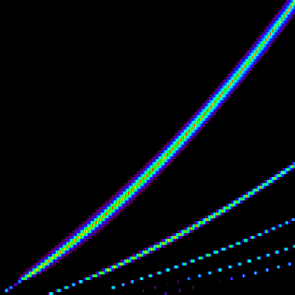
Figure 1: Response for the small-angle part of the RGS dispersion response. The plot shows input wavelengths (vertical axis) and $\beta$ (horizontal axis). Each line corresponds to a spectral order (first through fifth), the brightest one being the first order response. This plot is only the on-axis response. It varies as a function of off-axis position. The red region is where the response function is the highest, whereas the black regions are where the response function is low.

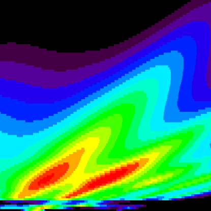
Figure 2: Response for the large-angle part of the RGS dispersion response. The plot shows input wavelengths (vertical axis with wavelength increasing) and $\beta$ (horizontal axis). Each peak corresponds to a spectral order (first through fifth), the brightest one being the first order response. Contrast this with the previous plot. This plot is only the on-axis response. It varies as a function of off-axis angle. The red region is where the response function is the highest, whereas the black regions are where the response function is low. The complex nature of the response function at the bottom of the plot is due to the gold M shell edge, which affects the reflectivity dramatically.

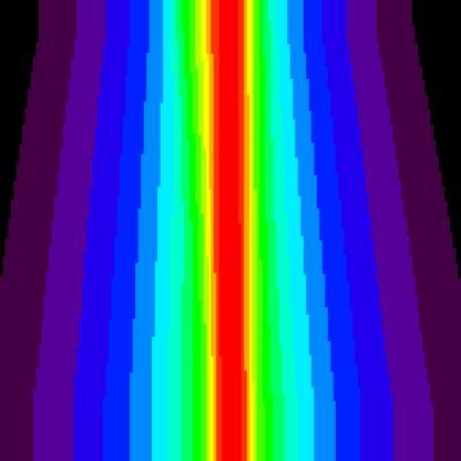
Figure 3: Response for the small-angle part of the RGS cross-dispersion response. The plot shows input $\beta$ (vertical axis with $\beta$ increasing) and cross-dispersion, $y$ (horizontal axis). This plot is only the on-axis response. It varies as a function of off-axis angle. The red region is where the response function is the highest, whereas the black regions are where the response function is low.

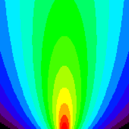
Figure 4: Response for the large-angle part of the RGS cross-dispersion response. The plot shows input wavelength (vertical axis with wavelength increasing) and cross-dispersion, $y$ (horizontal axis). This plot is only the on-axis response. It varies as a function of off-axis angle. The red region is where the response function is the highest, whereas the black regions are where the response function is low.

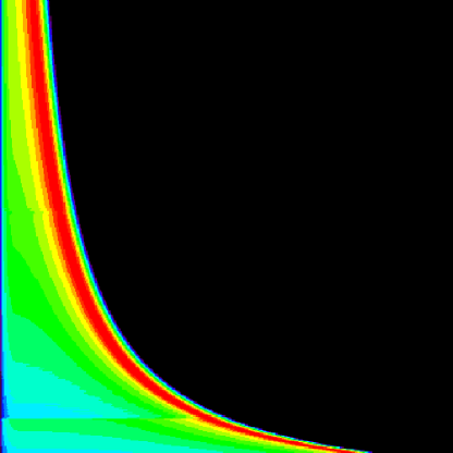
Figure 5: Response for the CCD pulseheight redistribution for a particular CCD node. The plot shows input wavelength (vertical axis with wavelength increasing) and pulseheight (horizontal axis). The red region is where the response function is the highest, whereas the black regions are where the response function is low. The horizontal shift in the response near the bottom of the plot corresponds with the silicon K shell edge.

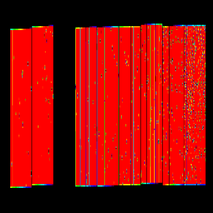
Figure 6: CCD exposure map showing the positions of the 9 CCDs. Unexposed areas included areas where there are hot pixels (points), hot columns(lines), and a failed CCD (missing area three from the left). The exposure map does not have sharp edges due to the correction of the small aspect drifts of the telescope. The exposure map is close to 1 in the red regions, whereas the exposure map is close to 0 in the black regions.

The pulseheight function, $h$, is the response of the various CCDs in the RFC. A separate response function is calibrated for each CCD as well as for each node of the CCD. The exposure map, $i$, is used to keep track of where the CCDs are located relative to one another as well as to remove locations of the angular space where there are bad pixels or columns. Aspect drift is included in its calculation. Its value is usually either close to one or zero depending on whether there is an active pixel at a given angular position. In addition to the six functions there is an overall normalization of the total effective area (units of $\mbox{cm}^{2}$) and a total exposure time of a given observation. The combination of these normalizations, the six functions, and a model spectrum in units of photons per $\mbox{cm}^{2}$ that can vary spatially, can be used to predict a given number of photons at a value of $\beta$, $y$, and $p$. We plot two-dimensional slices of these six functions in Figures 1-6. These can be calculated from the Science Analysis System (SAS) task rgsmcrgen (a task we designed explicitly for these Monte Carlo calculations) for the first five functions and rgsproc (the standard analysis pipeline) for the exposure map.

For an observation of an unresolved source, the calculations of the response function is straightforward. The substitution of equation 8 into equation 2 results in a integral relation like that of Equation 1. This is obtained after integrating over a given pulseheight and cross-dispersion selection. This integration only has to be performed once during an analysis. This is routinely done in the Science Analysis System (SAS) in the construction of response matrices in the task rgsrmfgen (the standard response generator). Then Equation 1 can be used in standard response matrix manipulations in software packages, such as XSPEC.

For a spatially-resolved X-ray source, complete integration of Equation 2 is unfeasible. Furthermore, additional approximations to reduce the dimensionality of Equation 8 are not possible without assuming that the source spectrum does not change as a function of spatial position, the response function does not change significantly at off-axis angles, and the lost events outside of a given pulseheight and cross-dispersion data selection is not significantly different than that of a point source, as we have discussed in §1. Although those three approximations can been applied in some global analyses of extended sources with the RGS (see either Rasmussen et al. 2001 (XSPEC model RGSXSRC) or Kaastra et al. 2001 (SPEX function)), we wish to avoid these assumptions in order to allow the spectral model to vary spatially. This will later give us much more flexibility in astrophysical modeling. The solution to the general problem presented here is the direct Monte Carlo integration of Equation 2 while using a novel scheme for interpolating between elements of the expression in Equation 8. We outline this technique as applied to the RGS below.

3 RGS Monte Carlo Response Calculation

Monte Carlo codes have always played an important role in the calibration of X-ray space observatories and in the simulation of complex observations. However, they have not achieved widespread use in data analysis applications, primarily because of slow computation speeds. Here we describe a method that generates events at rates of $10^{4}$ to $10^{5}$ photons per second per GHz of processor speed and apply it to the RGS response functions.

A photon can be generated through probability density functions, like the six functions described in section 2, in the following way. Let the probability of a photon being detected with an output value, $a$, given some input variable, $b$, be represented by a probability density function, $P(a~{}|~{}b)$, normalized to unity. We want to sample this distribution by obtaining a set of events with various values of $a$. First we calculate the cumulative distribution: $C(a)=\int_{-\infty}^{a}~{}da^{\prime}~{}P(a^{\prime}~{}|~{}b)$. Drawing a random number, $u$, between 0 and 1 then gives us a photon with a value of $a$ where $C(a)=u$. Photons can also be thrown away in order to maintain the proper normalization if the probability varies as a function of $b$.

We incorporate the above method in a two step process to compute the integral in Equation 2. First, photons are chosen using the model function, $S$, where the input variables, $b$, are the model parameters and the output variables, $a$, are the photon energy and sky coordinates ($e$, $\theta$, $\phi$). We then use a second Monte Carlo to predict sets of detector coordinates ($x$, $y$, $p$), using the sets of photon energies and sky coordinates as the input variables, $b$, and involving the response function, $R$, as the multi-dimensional probability distribution. The detailed implementation of the first step depends greatly on the type of astrophysical model, so we do not attempt to cover all cases here. The second step involves only the RGS instrument response, however, and is used in the same way for all observations and analyses. In the remainder of this section, we concentrate on ways of maximizing the efficiency of this second step.

The calculation of a single element of the response kernel, $R$, is computationally intensive, since $R$ is not described by simple analytic functions as we have discussed in §2. The response kernel can be pre-calculated, however, and stored at various grid points. This improves the speed of photon generation by several orders of magnitude over recalculating the response function for every photon. The RGS response function, however, contains many three dimensional functions requiring billions of elements at full resolution.

3.1 Interpolation Scheme

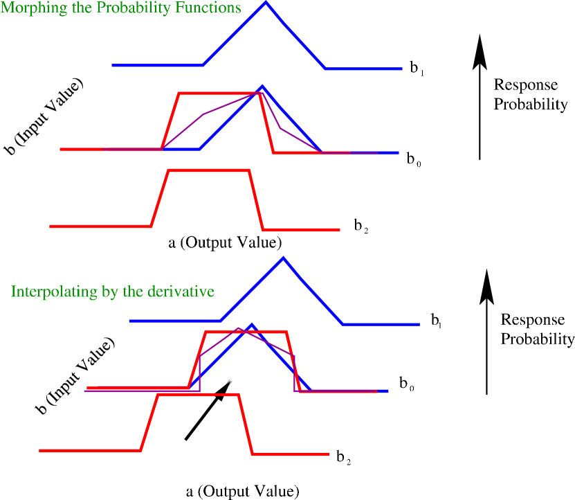
Figure 7: Schematic of the Monte Carlo interpolation method outlined in the text. In each of the two panels, we show a hypothetical response probability for a variable, a, that is dependent on some input variable, b. Instead of calculating the response probability for all possible values of b, we assume we have only calculated the response probability at $b_{1}$ and $b_{2}$ and then use an interpolation scheme to approximate the response probability at $b_{0}$. If the response peaks line up, we can simply use the probability distribution at $b_{1}$ and $b_{2}$ some fraction of the time as shown in the top panel and get a combined probability curve shown by the purple curve. The probability distributions can also be shifted if the response probability peaks do not have a common value as shown in the second panel.

Instead of saving the functions in Equation 8 in fine grids, we save the response kernel on coarse grids and then interpolate between grid points to obtain the intermediate values. Consider first the one-dimensional case, where we want to know the probability response function, $P(a~{}|~{}b)$, of some variable $a$, at some point, $b$. Assume that the response has been pre-calculated at positions $b_{1}$ and $b_{2}$ such that $b_{1}<b<b_{2}$. The response at position $b_{1}$ can be used as an approximation for the response at $b$ some fraction of the time and the response function at $b_{2}$ can be used the other fraction of the time. These fractions are determined by the distance that $b$ is from $b_{1}$ and $b_{2}$. A random number, $r$, is generated to determine which function to use. The response at $b_{1}$ is used if $r$ is greater than $\left(b-b_{1}\right)/\left(b_{2}-b_{1}\right)$. In this way, the intermediate probability function becomes a linear combination of the probability function at the two grid points after many photons are generated. This procedure is illustrated schematically in the top panel in Figure 7.

An additional step is needed if the response functions have sharp peaks that shift as a function of $b$. This is clearly the case for the dispersion function in Figure 1. The response peaks, however, can be shifted by interpolating by the derivative of the response function (i.e., the derivative of Equations 3-6). Say we choose to use the response at position $b_{1}$ by the random number $r$. Then after choosing a value of $a$ from that response function, we shift $a$ by $a\rightarrow a+\frac{da}{db}(b-b_{1})$. This shifts the response function as illustrated in the bottom panel in Figure 7. These two interpolation steps are, in general, much faster than the steps needed to calculate the response function. Such Monte Carlo interpolation methods are also easily generalized to more dimensions by drawing several random numbers, $r$, for each dimension and then shifting by each of the partial derivatives in each dimension. We will repeat this interpolation scheme several times using the specific RGS response functions in the following section.

3.2 Detailed Response Calculation Procedure

There are several steps in the Monte Carlo calculation that involve manipulating the functions described in §2 by the method outlined in §3.2. The goal of this calculation is to start with a set of sky angles ($\theta$, $\phi$) and wavelength, $\lambda$, for a given photon and end with a set of detected event coordinates, ($\beta$, $y$, and $p$). The first step of the RGS Monte Carlo is to choose one of the two instruments. This is accomplished by taking the sum of the normalization for $f_{SA}$ and $f_{LA}$ for RGS 1 and 2 separately. Then we draw a random number between 0 and 1 and choose the instrument based on the relative values of the two normalizations.

The second step is the correction for the instrument boresight. The RGS instruments are misaligned with respect to one another, so the sky coordinates, $\theta$ and $\phi$, are not trivially related to the $\theta$ and $\phi$ that we use in the instrument response functions. We therefore define $\theta_{ST}$, $\phi_{ST}$ as the sky angles relative to the star tracker and then convert these coordinates to a set of coordinates ($\theta$, $\phi$) for each RGS instrument. This is accomplished by a standard Euler transformation, such that the rotated coordinates, $r^{\prime}$, are related to the input vector, $r$, by

$$r^{\prime}_{i}=M_{ij}r_{j}$$ (9)

where $M$ is an approximately diagonal rotation matrix specified for each RGS. More details of this transformation can be found in Peterson (2003).

A third step chooses whether the photon follows the small-angle or large-angle response distribution. This is simply accomplished by taking the relative normalization of the $f_{SA}$ and $f_{LA}$ distribution and choosing based on that distribution. Assume first that we have chosen the large-angle distribution. Then, we find a $\beta$ for that photon by the following procedure. First, find the closest wavelength on the wavelength grid that defines $f_{SA}$. Define the difference between the closest wavelength, $\lambda_{1}$, and the desired input wavelength, $\lambda_{0}$, as $\Delta\lambda_{10}$ and the difference between the second closest wavelength, $\lambda_{2}$, and $\lambda_{0}$ as $\Delta\lambda_{20}$. Then we will use the reference wavelength, $\lambda_{1}$, if a random number is less than $\frac{\Delta\lambda_{20}}{\Delta\lambda_{10}+\Delta\lambda_{20}}$. Otherwise, we will use the reference wavelength $\lambda_{2}$. Define the reference wavelength that we have chosen as $\lambda_{i}$.

We repeat the same procedure for finding a reference $\theta$, which we define as $\theta_{i}$. Then we look up the cumulative probability distribution, $f_{SA}$, which is a function of $\beta$, for a given $\theta_{i}$ and $\lambda_{i}$. It will have a monotonically increasing value between 0 and 1 at each $\beta$. Note that the maximum value might be less than 1 because at a given $\lambda$ and $\theta$ since its value might be lower than at another $\lambda$ and $\theta$ where the response is higher. Then another random number, $r$, is chosen and we find the value of $\beta$ where $r=f_{SA}(\beta~{}\vline~{}\lambda_{i},\theta_{i})$. If the value of $r$ is greater than the maximum value for $f_{SA}$ then the photon is thrown away and we start the procedure over again. We, however, keep track of the number of photons that have been discarded.

Assume now that we have successfully chosen a value of $\beta$=$\beta_{0}$. Then, the final value of $\beta$ that will be output by the Monte Carlo is defined by

$$\beta=\beta_{0}-\frac{\cos{(\beta_{0})}-\cos{(\alpha_{0}+\theta_{0}\frac{L}{F})}}{\sin{\beta_{0}}}\frac{\lambda-\lambda_{0}}{\lambda_{0}}+\frac{\sin{(\alpha_{0}+\theta_{0}\frac{L}{F})}}{\sin{(\beta_{0})}}(\theta-\theta_{0})\frac{L}{F}$$ (10)

This equation is derived by differentiating the dispersion equation. A final step that avoids some aliasing is to shift that value of $\beta$ on to a uniform $\beta$ grid according to the same procedure where we found the reference $\theta$ and $\lambda$.

The fourth step consists of choosing the cross-dispersion value, $y$, based on the function, $g_{SA}$. We first choose the reference $\phi_{i}$ based on the same procedure we used to get the reference $\lambda$ or $\theta$ in the previous step. We also use the value of $\beta$ we obtained from the previous step. Then a random number, $r$, is chosen between 0 and 1 where we will find a value $y$ such that $r=g_{SA}(y~{}\vline~{}\phi_{i},\beta)$. There is some possibility that we will throw out this photon for sufficiently high values of $r$. Otherwise, we will end up with a value $y_{0}$. This value is shifted according to the equation,

$$y=y_{0}+\left(\phi-\phi_{i}\right)$$ (11)

Finally, we align $y$ according to a predefined reference grid according to the same procedure we have used to find our reference $\theta_{i}$. We now have a prediction for both the dispersion variable, $\beta$, and the cross-dispersion variable, $y$.

If we had chosen the large-angle distribution instead of the small-angle distribution at the beginning of step 3 the procedure is nearly identical. We first use the distribution $f_{LA}$ instead of $f_{SA}$ to get the value of $\beta$. Then we use $g_{LA}$ instead $g_{SA}$ to get the value of $y$. $f_{LA}$ depends on wavelength, however, rather than $\beta$. We then have a prediction for the values of $\beta$ and $y$ for the photons that are produced from the large angle part of the response as well.

The fifth step consists of using the exposure map to determine if the particular value of $\beta$ and $y$ corresponds with an active region of one of the CCDs. Each value of the exposure map, $e$ will have a value between 0 and 1. We then simply find the value of $i(\beta,y)$ and throw the photon away if the value of the exposure is less than a given random number chosen between 0 and 1. Otherwise, the photon is considered detected and we proceed to the final step.

The last step consists of choosing the CCD pulseheight distribution. The distribution is different for each of the two nodes for each CCD. Therefore using the chosen value of $\beta$ we determine which CCD node for the photon using a simple linear function. This is correct in the limit that the CCDs are approximately aligned in $\beta$, which is a good approximation although they are slightly rotated. Then, we choose a reference wavelength, $\lambda_{i}$, based on the wavelength grid for the function $h$ using the same procedure used in step 3 and 4. A random number, $r$, is chosen between 0 and 1. The predicted CCD pulseheight is then chosen by finding the value of the pulseheight distribution such that $r=h(p~{}\vline~{}\lambda_{i},\mbox{CCD~{}node})$. We then shift the value of the pulseheight by

$$p=p_{0}-\frac{hc}{\lambda}+\frac{hc}{\lambda_{i}}$$ (12)

If $r$ is greater than the value of $h$ then we throw the photon away. Otherwise, we have successfully predicted a value of $\beta$, $y$, and $p$.

The overall normalization is achieved by using the total number of photons we attempted to simulate, $N$, the maximum value of the effective area, $A$, the maximum value of the exposure map, $T$, and the relative normalization, $Q$, of the model in units of photons $\mbox{cm}^{-2}~{}\mbox{s}^{-1}$. If we simulate $m$ photons and there are $n$ photons in the data set, then the normalization of the spectral model is given by

$$\mbox{Normalization}=\frac{N}{Q~{}A~{}T}\times\frac{n}{m}.$$ (13)

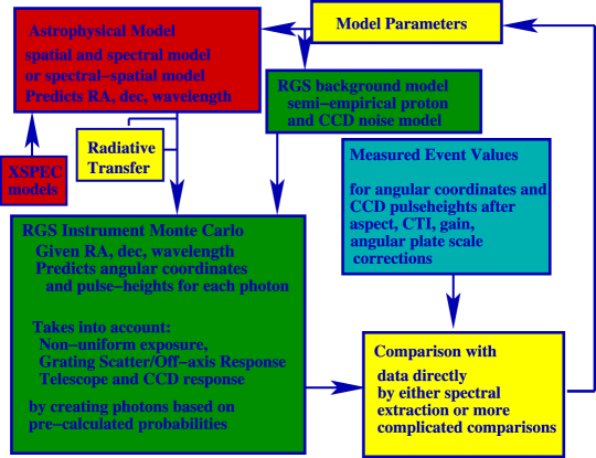
Figure 8: Flowchart of the Monte Carlo method used in this paper. See section 4 for a detailed explanation of each step.

The Monte Carlo generates photons at rates of $5000$ photons per second per GHz of processor speed. An example of a simulation of monochromatic light from a point source is shown in Figure 8 and 9. A public version of this code is currently being prepared.

4 Towards a General Method for Diffuse X-ray Spectroscopy

Given an efficient instrument response Monte Carlo, how can it be used with the measured data to constrain an astrophysical model? Schematically, the following steps are required:

• Models are formulated in terms of a set of parameters. These parameters predict probability distributions for the spectral and spatial distributions.

• Photons are then drawn from these probability distributions and assigned an energy and two sky coordinates ($\theta$, $\phi$).

• The detector coordinate and pulseheight values ($x$, $y$, $p$) are predicted from the instrument Monte Carlo.

• The simulated events are compared with the measured photon events via a comparison statistic.

• Finally, an iteration is performed to optimize this statistic subject to variation of the input parameters. When the iteration converges, the best fit has been found.

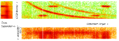
Figure 11: Raw RGS data for the galaxy cluster, Sérsic 159-03. The plot consists of three panels for each of the two-dimensional projections of the three dimensional data. The dispersion coordinate vs. cross-dispersion coordinate shows the dispersed spectral image. It is blurred in the cross-dispersion direction due to the size of the source. The three curved lines in the dispersion coordinate vs. CCD energy plot show the first, second, and third order dispersed spectra. The four horizontal lines are the Al K and F K calibration sources. Most of the photons in this image are due to Bremsstrahlung. A darker region in the first order curved line is due to Fe L lines. The red regions are high intensity regions, and the green regions is low intensity regions.

These steps are also outlined in Figure 10 and are similar to standard analysis methods practiced in high energy astrophysics. An example of a simulation and an actual data set for a galaxy cluster is in Figure 11 and 12.

5 RGS Event Comparison

Following, we discuss several useful methods of comparing the raw RGS data and the simulated photons from the Monte Carlo calculation like that in Figure 11 and 12. The obvious advantage of using a Monte Carlo is that we can manipulate and select the data in any way since we can perform the same operations to the simulated photons. For this reason there are a variety of approaches to event comparison. We have found that some are more useful depending on the situation.

5.1 Wavelength, Order, and Cross-dispersion Assignment

After simulating a set of photons with a set of values of $\beta$, $y$, and $p$, it is more convenient to convert those coordinates into a corrected wavelength, $\lambda^{\prime}$, cross-dispersion value, $\phi^{\prime}$, and spectral order (the $\prime$ designates that this may not be the true wavelength but the one measured by the RGS). This is accomplished by using Equation 3 with the value of $\beta$ and cross-dispersion relation with the value of $y$ after using the pulseheight $p$ to determine whether the photon falls into first, second, or third order. We assume a nominal dispersion coordinate, $\theta$, for all of the photons even though for an extended source we may not have the same input $\theta$ for every event. We can do this because we can perform the same operations the simulated data. We can interpret a shift in wavelength from a spectral line as either an actual wavelength shift or a shift caused by the finite extent of the source.

5.2 Data Selection: Order selection and cross-dispersion cuts

A simple yet important step of a Monte Carlo is the selection of data. We can perform the same data selection cuts that are normally performed on point source observations. A selection in cross-dispersion is achieved by requiring all values of $\phi^{\prime}$ between an arbitrary $\phi_{1}$ and $\phi_{2}$ such that $\phi_{1}<\phi^{\prime}<\phi_{2}$. Similarly, a joint pulseheight-dispersion cut is achieved by requiring that the pulseheight, $p$, falls within the window $\frac{hc}{\lambda^{\prime}}\pm\sqrt{a+b\frac{hc}{\lambda^{\prime}}}$ for some arbitrary constants $a$ and $b$. With extended sources, the joint dispersion-pulseheight cut is also broadened by calculating the above formula based on two values of $\theta$ and then making sure the pulseheight value in within in the window for both values of $\theta$. These selection cuts are important to reduce the number of background events. The advantage of using the Monte Carlo is that events can quickly be sorted and removed if they do not satisfy the selection criteria. The selection can be changed arbitrarily without re-running the simulation. Cross-dispersion cuts, in particular, can be used to compare different spatial regions.

5.3 Two-Sample $\chi^{2}$

Various statistics can be constructed to determine the quality of the model used in the simulation. In particular, a useful specific form of the $\chi^{2}$ statistic for two samples of data can be computed. This is given below for binned data where the number of events in the $j$th bin for the data photons is $V_{1j}$ and for the model photons is $V_{2j}$. If there are $n$ total events in the data and $m$ simulated events in the model then the $\chi^{2}$ statistic is given by

$$\chi^{2}=\sum_{j}\frac{~{}|~{}V_{1j}-\frac{n}{m}V_{2j}~{}|~{}^{2}}{\frac{n}{m}(V_{1j}+V_{2j})}.$$ (14)

Note that the two sample $\chi^{2}$ value approaches the familiar continuous form of $\chi^{2}$ when $V_{2j}$ is replaced with $mP$ where P is the probability model and $m\rightarrow\infty$.

The two-sample $\chi^{2}$ is used to compare both the extracted spectra (a binned histogram of $\lambda^{\prime}$) and the cross-dispersion distribution (a binned histogram of $\phi^{\prime}$). They are both extremely useful in comparing the spectrum to the model spectrum and the cross-dispersion distribution compared to the predicted one. In Peterson et al. (2001) and Peterson et al. (2003) this method was employed to compare several spectra and the cross-dispersion distribution iteratively. It is also possible to compute a two-dimensional $\chi^{2}$ statistic on the binned wavelength-cross-dispersion data space. This is only possible with extremely bright sources, however, since there are usually a few counts per bin.

5.4 Two-Sample Cramér von Mises

We have also found an alternative statistic useful when using comparing RGS data. The Cramér-von Mises statistic, $W^{2}$ (Anderson and Darling 1952), which is a more robust version of the Kolmogorov-Smirnov statistic (Smirnov 1948), is determined by computing the cumulative distribution of the data values, $C_{1}$, and the model values, $C_{2}$, and then evaluating the following sum at each of the model and data values,

$$W^{2}=\frac{mn}{{\left(m+n\right)}^{2}}\sum_{{\rm{data~{}and~{}model~{}values}}}{|C_{1}-C_{2}|}^{2}.$$ (15)

The statistic is most easily computed by sorting the data and model values. The statistic can be extended to multi-dimensional distributions by comparing values that are a linear combination of the value in each dimension. If we compute the Cramér-von Mises statistic of $v$ where $v=a_{1}\beta+a_{2}y+a_{3}p$, then we can compare the multi-dimensional distribution. The Cramér-von Mises statistic is computed for a set of several $(a_{1},a_{2},a_{3})$ so that the value in one-dimension is emphasized more than other dimensions in each computation. If enough combinations are used, the statistic is relatively insensitive to our choice of $a_{i}$. We have used this method to compare the multi-dimensional distribution of the background. It works well for this purpose since few photons fill each bin of the three-dimensional ($\beta$, $y$, $p$) space. It may be possible to construct other useful two-sample multi-dimensional statistics as well and clearly there is more progress to be made in this area.

6 Extensions of the Method

Below we discuss several extensions to the method.

6.1 Iteration Scheme

We have not yet discussed methods for iterating the model parameters after the photons have been simulated and the statistics have been calculated. One method involves changing the parameters of the model after all the photons have been simulated. The standard techniques for the iteration of a set of model parameters without using a Monte Carlo are applicable here as well. Simplex (O’Neill 1971), simulated annealing, Markov chain Monte Carlo techniques, or robust grid searches may be the best methods since they all avoid using derivatives of the fitting statistic and therefore avoid the statistical $\sqrt{m}$ fluctuations of the Monte Carlo.

A more advanced form of iteration involves selecting individual photons produced from a set of parameters that improve the statistic. The statistic is evaluated after every photon is produced instead of after the entire set is simulated. This is then the Monte Carlo analog to deconvolution as opposed to model fitting. Further discussion of this technique is described in Jernigan and Vezie (1996) and Jernigan, Peterson, & Kahn (2004).

6.2 Error Analysis

Systematic errors dominate over statistical errors in many of the multi-dimensional global fits we have considered here. Additionally, the statistics we have discussed in §5.1 usually have a non-universal distribution. Our focus in using these statistics is merely for model iteration and not for hypothesis testing or for constructing parameter confidence regions.

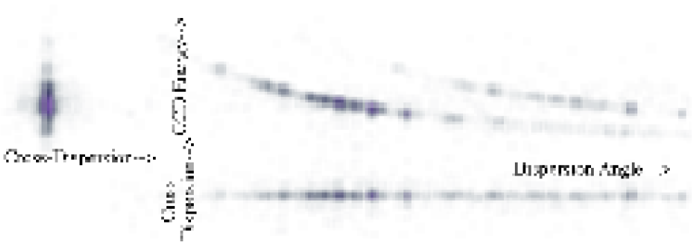
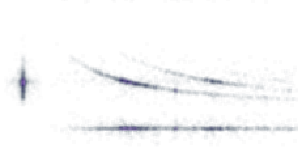
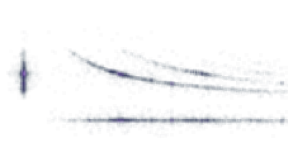
Figure 13: (Three panels) Three simulations of a thermal plasmas at electron temperatures of 0.5, 1.0, and 1.5 keV emitted from an unresolved source using the RGS Monte Carlo. Each plot is segmented in the same way as in Figure 11 and 12. The bright spots represent photons from strong emission lines. The simulations are compared in Figure 14. Each simulation has approximately 30,000 photons.

Standard parameter estimation techniques, however, can still be applied when dealing with the one-dimensional spectrum or a specific feature in the data. For example, one can first calculate $\chi^{2}$ on the one-dimensional extracted spectrum of both the data and simulation as in §4.2. Then the difference in $\chi^{2}$ when a parameter is varied can be estimated. This method is identical to standard parameter estimation techniques in X-ray astronomy (Lampton, Margon, & Bowyer 1976). A simple example of this is shown in Figure 13 and 14. In some other circumstances, however, bootstrapping techniques (Efron 1979) could be used to construct the distribution of these multivariate statistics when statistical errors dominate.

6.3 Other Instruments and Background

Although we have focused on a number of multivariate Monte Carlo methods for the Reflection Grating Spectrometer, there is little in our discussion that could not be generalized to analysis of data from other instruments as well. The three dimensional structure of the response calculation is not unlike the structure of a non-dispersive instrument response that has an energy-dependent point-spread function, vignetting function, CCD response function, and an exposure map. The flexibility in astrophysical modeling of this approach may outweigh the advantages of the simplicity of traditional one-dimensional spectral extraction techniques at least in some situations. We have also applied this method to a Monte Carlo of the RGS background induced by charged particles and other instrumental sources. The background Monte Carlo has its own response function that differs from equation 8. For more details about this Monte Carlo see Peterson (2003).

6.4 Further Astrophysical Modeling

After the instrument response is formulated as a Monte Carlo it is reasonable to consider more complicated astrophysical modeling that could involve a Monte Carlo approach. A flexible method is to formulate the astrophysical models always in three dimensions and then project the photon velocity shifts and spatial positions to the two dimensional sky coordinates. Radiative transfer also becomes a straight-forward problem since individual photons can have their frequency shifted or trajectory altered. Monte Carlo techniques for this are well-developed, but these techniques can be used naturally in conjunction with a Monte Carlo treatment of the instrument model as in Xu et al. (2001). We expect that many of the methods discussed here could allow a closer connection between future observational and theoretical work.

6.5 Acknowledgements

We thank an anonymous referee for many important comments that greatly improved this manuscript. JRP acknowledges many helpful discussions and technical improvements to the Monte Carlo code and methods by Jean Cottam, Maurice Leutenegger, Frits Paerels, Andy Rasmussen, Doug Reynolds, Masao Sako, Cor de Vries, and Haiguang Xu, as well as additional support from the XMM-RGS team and the XMM collaboration. SMK acknowledges partial support for this work under SAO Chandra grant GO2-3178X.

Figure 9: Simulation of a set of 10 Å photons. The plot shows the cross-dispersion vs. dispersion histogram. The left peak is the first order spot and the right peak is the second order spot. Large scattering wings are present off a sharply peaked core. Red shows the high intensity regions, and green shows the low intensity regions.

Figure 10: Simulation of a set of 10 Å photons. The plot shows the pulseheight vs. dispersion histogram. The left peak is the first order spot and the right peak is the second order spot. Large scattering wings are present off a sharply peaked core along the dispersion direction and the partial event tails of the pulseheight distribution extend vertically. Red represents the high intensity regions, and green represents the low intensity regions.

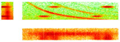
Figure 12: The same plot as Figure 11 except the photons are simulated by a model using a Monte Carlo. Details of the simulation can be found in Peterson et al. (2003a). The green represents low intensity regions, and the red represents high intensity regions.

Figure 14: The two-sample $\chi^{2}$ and the Cramér-von Mises statistic, $W^{2}$, (see text) calculated on the one-dimensional extracted spectrum by comparing the 1 keV simulation in Figure 13 with various other simulations at other temperatures. The statistics correctly achieve the minimum at 1 keV and fluctuate around their 50th percentile values (1.0 for $\chi^{2}$ and 0.12 for $W^{2}$). The fluctuations can be diminished if more events are simulated.

References

- Arnaud (1996) Arnaud, K. A. 1996, Astronomical Data Analysis Software and Systems V ASP Conference Series, Vol. 101, George H. Jacoby and Jeannette Barnes, eds.
- Arnaud et al. (2001) Arnaud, M., Neumann, D. M., Aghanim, N., Gastaud, R., Majerowicz, S., and Hughes, J. P. 2001, A & A 365, L80-86.
- Anderson and Darling (1952) Anderson, T. W. and Darling, D. A., Annals of Mathematical Statistics, Volume 23, Issue 2, Jun. 1952, 193-212.
- den Herder et al. (2001) den Herder, J. W. et al. 2001, A & A 365, 7.
- Gorenstein, Gursky, & Garmire (1968) Gorenstein, P., Gursky, H., & Garmire, G. 1968, ApJ 153, 885.
- Efron (1979) Efron, B., Annal. Stat. 1979, 7, 1.
- Jansen et al. (2001) Jansen, F. et al. 2001, A&A 365, 1.
- Jernigan and Vezie (1996) Jernigan, J. G. & Vezie, M., Astronom. Data Analysis Software and Systems V, ASP Conference Series, Vol 101. 1996.
- Jernigan, Peterson, & Kahn (2004) Jernigan, J. G., Peterson, J. R., & Kahn, S. M., in preparation.
- Kaastra et al. (2001) Kaastra, J. S. et al.. 2001, A & A 365, 99.
- Kaastra et al. (1996) Kaastra, J. S., Mewe, R., & Nieuwenhuijzen, H. 1996, in “UV and X-ray Spectroscopy of Astrophysical and Laboratory Plasmas”, Tokyo: Universal Academy Press.
- Kahn et al. (1996) Kahn, S. M., Cottam, J., Decker, T. A. et al. 1996, Proc. SPIE 2808, 450.
- Kahn & Hettrick (1985) Kahn, S. M. & Hettrick, M. C. 1985, in ESA Proceedings of a ESA Workshop for a Cosmic X-ray Spectroscopy Mission, Paris: ESA, 237.
- Lampton, Margon, & Bowyer (1976) Lampton, M., Margon B., & Bowyer, S. 1976, ApJ 208, 177.
- Markevitch & Vikhlinin (2001) Markevitch, M. & Vikhlinin, A. 2001, ApJ 563, 95.
- Metropolis & Ulam (1949) Metropolis, N. & Ulam, S. 1949, J. A. S. A. Vol 44, 335.
- O’Neill (1971) O’Neill R., Applied Statistics, Vol 20, Issue 3, 1971, 338-345.
- Peterson et al. (2001) Peterson, J. R. et al. 2001, A&A 365.
- Peterson et al. (2003) Peterson, J. R. et al. 2003, ApJ 590, 207.
- Peterson (2003) Peterson, J. R. 2003, PhD Thesis, Columbia University.
- Rasmussen et al. (1998) Rasmussen, A. et al. 1998, SPIE 3444, 327.
- Rasmussen et al. (2001) Rasmussen, A. et al. 2001, A & A 365, 231.
- Smirnov (1948) Smirnov, N., Annals of Mathematical Statistics, Vol 19, Issue 2, 279-281, June 1948.
- Weisskopf et al. (2000) Weisskopf, M., Tannenbaum, T., Van Speybroeck, L., O’Dell, S. L. 2000, Proc. SPIE Vol. 4012, 2-16.
- Xu et al. (2001) Xu, H. et al., 2002, ApJ 576, 600.