Magnetic Field Generation in Fully Convective Rotating Spheres

Abstract

Magnetohydrodynamic simulations of fully convective, rotating spheres with volume heating near the center and cooling at the surface are presented. The dynamo-generated magnetic field saturates at equipartition field strength near the surface. In the interior, the field is dominated by small-scale structures, but outside the sphere by the global scale. Azimuthal averages of the field reveal a large-scale field of smaller amplitude also inside the star. The internal angular velocity shows some tendency to be constant along cylinders and is “anti-solar” (fastest at the poles and slowest at the equator).

1. Introduction

The Hayashi track in the Hertzsprung–Russell diagram characterizes young stars in hydrostatic equilibrium that are fully convective. Other fully convective stars are low-mass main sequence stars (M dwarfs), and some cool giants. These stars show strong magnetic activity as is evidenced by chromospheric emission in H$\alpha$ (e.g. Hawley, 1993; Hawley et al., 1999) and by Zeeman broadening of classical T Tauri stars (e.g. Johns-Krull et al., 1999b). In the latter case, the stars are generally rapidly rotating with rotation periods of just a few days, and it is known that the magnetic field shows strong departures from axisymmetry (Johns-Krull et al., 1999a). However, for less massive stars (M9 dwarfs and beyond) there is a sharp decline in chromospheric magnetic activity (e.g. Gizis et al., 2000), which may be connected with dust formation and the almost fully neutral photospheres (Mohanty & Basri, 2003).

Despite some progress in low-resolution Doppler imaging (e.g. Joncourt et al., 1994), not much is known about the surface differential rotation of these stars, and even less is known about their internal angular and meridional velocities. Theory suggests that the absolute differential rotation in fully convective stars decreases with increasing overall angular velocity due to rotational quenching of the turbulent transport effect that causes the differential rotation (Küker et al., 1993; Kitchatinov et al., 1994; Küker & Rüdiger, 1997, 1999). As in the solar case, the equator is still predicted to rotate more rapidly than the poles. However, some observations of rapidly rotating stars support what is sometimes referred to as “anti-solar” differential rotation, where the equator spins less rapidly than the poles (Barnes et al., 2004; Kitchatinov & Rüdiger, 2004; Weber et al., 2005). Since differential rotation enters as an important ingredient in dynamo theory, it is important to develop self-consistent models of the large-scale velocity field in fully convective stars.

Magnetic field generation in fully convective stars is also interesting from a dynamo theoretical point of view. With the realization that the magnetic field inside stars might be highly intermittent and concentrated in thin flux tubes, the question of storing such intermittent and strongly buoyant magnetic fields over the course of the 11 year cycle became a growing concern (e.g. Moreno-Insertis, 1983). This led to the proposal that dynamos in convective shells (as in the case of the Sun) might operate at or below the bottom of the convection zone. This scenario would not be applicable to fully convective stars, because they lack the overshoot layer where strong flux tubes could be stored. However, it is known that the chromospheric activity does not disappear for later spectral types, i.e. towards fully convective stars (Vilhu, 1984; Vilhu et al., 1989; Berger et al., 2005). It has therefore been claimed (Durney et al., 1993; Hawley et al., 2000) that fully convective stars lack large-scale magnetic fields, but can still have small-scale fields generated by non-helical near-surface turbulent dynamo processes.

Attempts to model such small-scale dynamo action (Dorch & Ludwig, 2002) have however led to the conclusion that the photospheric conductivities of M-dwarfs are most probably too low to allow for local small-scale dynamo action This would imply that the observed magnetic activity must be due to dynamo action in deeper layers.

From a kinematic mean-field $\alpha^{2}$ dynamo model, Küker & Rüdiger (1999) predicted that rapidly rotating (Coriolis number of 3 or larger) fully convective stars generate a non-axisymmetric steady magnetic field of quadrupolar symmetry and azimuthal order $m=1$ that looks roughly like a dipole field with the dipole axis lying in the equatorial plane.

Global models of convective dynamos are still in their infancy, even though some tremendous progress was made some 20 years ago when Gilman (1983) and Glatzmaier (1985) presented the first simulations of dynamos in a spherical shell representing a solar-like convection zone. These models predicted cyclic magnetic fields propagating toward the poles, in contrast to the solar case. The reason for this discrepancy remains a matter of debate even today, when much higher numerical resolution is available. Recent simulations still predict angular velocity to be roughly constant on cylinders, although some simulations show at least a tendency toward solar-like angular velocity contours (Miesch et al., 2000; Brun & Toomre, 2002). Recent simulations of dynamo action in spherical shells now begin to produce useful models of global turbulent dynamos (Brun, 2004; Brun et al., 2004). Meanwhile, such global models have also been applied to core convection (Browning et al., 2004) and to dynamo action in these cases (Brun et al., 2005).

In this paper, we present global dynamo simulations in spheres using a Cartesian grid, i.e. the sphere is embedded in a cubic box. This may seem to be an unnatural approach to spherical geometry, but it has distinct practical advantages. First, it avoids the coordinate singularity at the center when using spherical coordinates, without invoking expensive transformations from and to spherical harmonics. Second, this approach has proven useful in view of computational simplicity and numerical parallelization efficiency; it has recently been applied by a number of groups to purely hydrodynamic simulations (Porter et al., 2000; Freytag et al., 2002; Woodward et al., 2003), and attempts have already been made to model dynamo action in this approach (Dorch, 2004).

2. The Model

2.1. Basic setup

In our model the star is described as a spherical subregion of radius $R$ of a cubic box of size $L_{\rm box}^{3}$. The gas in the box is governed by the usual equations of magnetohydrodynamics (see below) with impenetrable boundaries on the box faces such that the mass $M_{\rm box}$ in the box is conserved. If the gravitational well $\Phi(r)$ is sufficiently deep, most of the mass $M$ of the star is concentrated near the center, so $M\approx M_{\rm box}$. Using a Newtonian cooling term in the energy equation, the temperature outside the star is kept close to the nominal surface temperature of the star, $T_{\rm surf}$. An entropy gradient is maintained by prescribing a distributed energy source $\mathcal{H}(r)$ at the center (here $r$ is the spherical radius). The total luminosity is then given by $L=4\pi\int_{0}^{R}\mathcal{H}(r)r^{2}{\rm d}{}r$, and corresponds to the energy produced by nuclear burning. We recall however, that some young stars on the Hayashi track have not ignited yet, and are sustaining their energy losses by contraction, which results in a less localized energy source than nuclear fusion reactions. Although the mass distribution can change during the evolution of our model, we have chosen to ignore self-gravity.

The model is governed by five main input parameters: mass $M$, radius $R$, luminosity $L$, surface temperature $T_{\rm surf}$, and average angular velocity $\Omega_{0}$. We choose parameters that are typical of M dwarfs, but we limit the degree of stratification to values that are numerically more feasible by choosing a surface temperature that is much higher than for real M dwarfs. We also keep the Kelvin-Helmholtz time scale at a much smaller multiple of the dynamical time scale than what is realistic. As is common in deep convection simulations (e.g., Chan & Sofia, 1986; Brandenburg et al., 2005), we do this by choosing a luminosity that is much larger than the stellar value, and at the same time we keep the radiative diffusivity much larger than in reality. Since the Rayleigh number is, for a given Prandtl number, inversely proportional to the square of the radiative diffusivity, a large luminosity translates to a small Rayleigh number. The restriction to moderate values of the Rayleigh number is a common problem of all astrophysically meaningful convection simulations.

Our initial state is derived from a spherically symmetric, isentropic reference model; for details see Appendix A. This state is perturbed by adding weak velocity and magnetic fields that are both random.

2.2. Equations

In the computational domain, $-L_{\rm box}/2\leq x,y,z\leq L_{\rm box}/2$, we solve the equations of compressible magnetohydrodynamics,

$$\frac{\mathrm{D}\ln\varrho}{\mathrm{D}t} = -\mbox{\boldmath{$\nabla$}}\cdot\mathbf{u}\;,$$ (1)

$$\frac{\mathrm{D}\mathbf{u}}{\mathrm{D}t} = -\frac{\mbox{\boldmath{$\nabla$}}p}{\varrho}+\frac{\mathbf{j}\times\mathbf{B}}{\varrho}+\frac{2}{\varrho}\mbox{\boldmath{$\nabla$}}\cdot\left(\varrho\nu\mbox{\boldmath{$\mathsf{S}$}}\right)$$ (2)

$$\mbox{}-\mbox{\boldmath{$\nabla$}}\Phi-2\mbox{\boldmath{$\Omega$}}_{0}\times\mathbf{u}+\mathbf{f}_{\rm d}\;,$$

$$\frac{\partial\mathbf{A}}{\partial t} = \mathbf{u}\times\mathbf{B}-\eta\mu_{0}\mathbf{j}\;,$$ (3)

$$\varrho T\frac{\mathrm{D}s}{\mathrm{D}t} = \mathcal{H}-\mathcal{C}+\mbox{\boldmath{$\nabla$}}\cdot(K\mbox{\boldmath{$\nabla$}}T)$$ (4)

$$\mbox{}+\mu_{0}\eta\mathbf{j}^{2}+2\varrho\nu\mbox{\boldmath{$\mathsf{S}$}}^{2}\;,$$

where $\varrho$ and $p$ denote mass density and pressure of the fluid, $s$ and $T$ are specific entropy and temperature, $\mathbf{u}$ is the fluid velocity, $\nu$ the kinematic viscosity, $\Phi$ the gravity potential, $\mbox{\boldmath{$\Omega$}}_{0}$ the angular velocity of the reference frame, $\mathbf{f}_{\rm d}$ is an artificial damping force discussed in Sec. 2.3, and

$$\mathsf{S}_{ik}=\frac{1}{2}\left(\frac{\partial u_{i}}{\partial x_{k}}+\frac{\partial u_{k}}{\partial x_{i}}-\frac{2}{3}\delta_{ik}\mbox{\boldmath{$\nabla$}}\cdot\mathbf{u}\right)$$ (5)

is the traceless rate-of-strain tensor. The magnetic vector potential $\mathbf{A}$ is related to the flux density $\mathbf{B}=\mbox{\boldmath{$\nabla$}}\times\mathbf{A}$ and the current density $\mathbf{j}=\mbox{\boldmath{$\nabla$}}\times\mathbf{B}/\mu_{0}$, and $\eta$ denotes the magnetic diffusivity. Volume heating $\mathcal{H}$ and cooling $\mathcal{C}$ are described in Sec. 2.3 below. The radiative conductivity $K$ is related to the thermal diffusivity $\chi\equiv K/(c_{p}\varrho)$. In the numerical calculations shown below, we assume $\chi$, $\nu$, and $\eta$ to be constant across the whole box. Our equation of state is that of a perfect gas with adiabatic index $\gamma=5/3$.

For the gravity potential $\Phi(r)$ we choose a Padé approximation obtained from our isentropic reference model (see Appendix A),

$$\Phi(r)=-\frac{GM}{R}\frac{a_{0}+a_{2}r^{\prime 2}+a_{3}r^{\prime 3}}{1+b_{2}r^{\prime 2}+b_{3}r^{\prime 3}+a_{3}r^{\prime 4}}\;,$$ (6)

with $r^{\prime}\equiv r/R$; we find that the coefficients, $a_{0}=2.34$, $a_{2}=0.44$, $a_{3}=2.60$, $b_{2}=1.60$, $b_{3}=0.21$, yield a good approximation both inside and outside the star.

Note that, while retaining the Coriolis force term, we neglect the centrifugal force. This is necessary for practical reasons, since together with the luminosity our turbulent velocities $u_{\rm rms}$ are exaggerated and we thus need far too large angular velocities in order to reach realistic Coriolis numbers [see Eq. (13) below]. It would therefore be unrealistic to include the strongly exaggerated centrifugal force in the expression for the inertial forces. We emphasize that this kind of restricted mechanics does not violate the balance of angular momentum $\mathbf{L}$ in any significant manner: The component $L_{z}$ parallel to the rotation axis is strictly conserved (the centrifugal force is a central force for that axis), while the other two components are small for a nearly axisymmetric system.

Our boundary conditions on the faces of the cubic box are impenetrable free-slip conditions for velocity ($u_{n}=0$, $\partial_{n}\mathbf{u}_{\rm tan}=\mathbf{0}$), and normal-field conditions for the magnetic field ($\partial_{n}B_{n}=0$, $\mathbf{B}_{\rm tan}=\mathbf{0}$).

All numerical calculations were done using the Pencil Code, a high-order centered finite-difference code (sixth order in space and third order in time) for solving the compressible hydromagnetic equations. Weak shock-capturing viscosities were used to cope with localized, transient events of supersonic flow. A high-order upwind scheme is used for the advection operators for density and entropy; see Appendix B.

2.3. Profile functions

As outlined in Sec. 2.1, the thermal structure of the star is maintained by prescribing a certain distribution of heating and cooling functions inside and outside the star, respectively. The profile functions depend on spherical radius $r\equiv(x^{2}{+}y^{2}{+}z^{2})^{1/2}$. In the exterior, $r>R$, we add a velocity damping term in order to prevent excessive velocities outside the star, which are not directly relevant to the dynamics inside the star.

Figure 1.— Comparison of luminosity function $L_{r}(r)\equiv\int_{0}^{r}\mathcal{H}(r^{\prime})\,4\pi r^{\prime 2}\,dr^{\prime}$ according to Eq. (A4) (dashed line) with our Gaussian parameterization (7). The choice $w_{\rm L}=0.162\,R$ gives an excellent fit, while the narrower profile would be more appropriate for a heavier star.

The central parts of the sphere are heated according to a normalized Gaussian profile,

$$\mathcal{H}(r)=\frac{L}{(2\pi w_{L}^{2})^{3/2}}e^{-r^{2}/(2w_{L}^{2})}\;,$$ (7)

which gives an excellent fit to the heating rate calculated according to Eq. (A4) for our isentropic reference model if the width $w_{L}$ of the nuclear burning region is chosen as $w_{L}=0.162\,R$. Fig. 1 shows a comparison of the resulting luminosity from the two parameterizations. Most of our simulations use that value of $w_{\rm L}$, while some runs have been carried out with $w_{\rm L}=0.1\,R$, which would be more appropriate for a more massive star.

For $r>R$, we apply a Newtonian cooling term of the form

$$-\mathcal{C}(r)=-\varrho c_{p}\,\frac{T{-}T_{\rm surf}}{\tau_{\rm cool}}\,f_{\rm ext}(r)$$ (8)

to keep the temperature close to the surface value $T_{\rm surf}$. Here, $f_{\rm ext}(r)$ is a profile function that smoothly interpolates between $0$ for $r\ll R$ and $1$ for $r\gg R$. Our profile function is a $\tanh$ profile,

$$f_{\rm ext}(r)=\frac{1}{2}\Bigl{(}1+\tanh\frac{r{-}R_{\rm cool}}{w_{\rm cool}}\Bigr{)}\;,$$ (9)

where $R_{\rm cool}$ and $w_{\rm cool}$ denote the position and width of the transition. We have chosen $w_{\rm cool}=0.05\,R$, and $R_{\rm cool}=1.05\,R$, i.e. slightly larger than the stellar radius, in order to reduce the influence of the cooling term (8) inside the star. In the present model, the exterior has practically constant temperature ($=T_{\rm surf}$), i.e. no attempt is made to model the hot corona of the star. In fact, since we have to restrict ourselves to moderate stratification, the temperature ratio between the center and the surface of the model is less than 10.

Table 1Summary of runs discussed in the paper.

Run	resol.	$\nu$	$\chi$	$\eta$	$\mathcal{L}$	$\Omega_{0}$	$\lambda$	$u_{\rm rms}^{\rm kin\,/\,sat}$	$B_{\rm rms}^{\rm sat}$	$\frac{B_{\rm rms}}{u_{\rm rms}}$	$\mathrm{Re}$	$\mathrm{Rm}$
1a	$128^{3}$	$6\times 10^{-4}$	$4\times 10^{-4}$	$3\times 10^{-4}$	$0.02$	$0.2$	$0.017$	$0.173$ / $0.164$	$0.020$	$0.12$	$273$	$547$
1b	$256^{3}$	$4\times 10^{-4}$	$3\times 10^{-4}$	$2\times 10^{-4}$	$0.02$	$0.2$	$0.043$	$0.184$ /	$0.028$	$0.18$	$388$	$775$
1c	$256^{3}$	$4\times 10^{-4}$	$3\times 10^{-4}$	$2\times 10^{-4}$	$0.01$	$0.2$		/ $0.130$	$0.023$	$0.18$	$325$	$650$
2a	$128^{3}$	$8\times 10^{-4}$	$8\times 10^{-4}$	$4\times 10^{-4}$	$0.02$	$0.0$	$0.009$	$0.239$ / $0.233$	$0.018$	$0.08$	$291$	$583$
2b	$128^{3}$	$8\times 10^{-4}$	$8\times 10^{-4}$	$4\times 10^{-4}$	$0.02$	$0.5$	$0.017$	$0.213$ / $0.185$	$0.046$	$0.25$	$231$	$463$
2c	$128^{3}$	$8\times 10^{-4}$	$8\times 10^{-4}$	$4\times 10^{-4}$	$0.02$	$2.0$	$0.021$	$0.158$ / $0.129$	$0.068$	$0.53$	$161$	$323$
2d	$128^{3}$	$8\times 10^{-4}$	$8\times 10^{-4}$	$4\times 10^{-4}$	$0.02$	$5.0$	$0.036$	$0.112$ / $0.087$	$0.099$	$1.14$	$109$	$218$
2e	$128^{3}$	$8\times 10^{-4}$	$8\times 10^{-4}$	$4\times 10^{-4}$	$0.02$	$10.0$	$0.038$	$0.086$ / $0.068$	$0.105$	$1.54$	$85$	$170$

Note. — Diagnostic quantities listed are: kinematic growth rate $\lambda$ of the magnetic field; root-mean-square values of velocity and magnetic flux density $u_{\rm rms}$, $B_{\rm rms}$; ratio $B_{\rm rms}/u_{\rm rms}$ for the saturated state; kinetic Reynolds number $\mathrm{Re}$ (based on $u_{\rm rms}$); and magnetic Reynolds number $\mathrm{Rm}$ (based on $u_{\rm rms}$). For all runs shown here, the star is embedded in a cubic box of size $L_{\rm box}=3\,R$. The gaps for Runs 1b and 1c are due to the fact that we have not extended Run 1b into the final saturated regime, but rather lowered the value of $\mathcal{L}$ and continued it as Run 1c.

Outside the star, a damping term

$$\mathbf{f}_{\rm d}=-\frac{\mathbf{u}}{\tau_{\rm d}}f_{\rm ext}(r)$$ (10)

is applied in the equation of motion to limit flow speeds to moderate values while still allowing the exterior to react to sudden disturbances from the stellar surface with sufficient flexibility; the profile $f_{\rm ext}(r)$ is the same as for the cooling term, i.e. Eq.(9) with $w_{\rm d}=0.05\,R$, and $R_{\rm d}=1.05\,R$. By imposing fixed radial profile functions for surface cooling and velocity damping, we suppress the possibility of irregular surfaces that would develop, e.g. in red giants (Freytag et al., 2002), but this would not apply to real M dwarfs.

2.4. Dimensionless parameters

As mentioned in the beginning, our model is governed by the five basic input parameters: $M$, $R$, $L$, $T_{\rm surf}$, and $\Omega_{0}$. From these, we can construct three dimensionless quantities that characterize our model: the stratification parameter

$$\xi\equiv\frac{c_{\rm s,surf}^{2}/\gamma}{GM/R}\;,$$ (11)

(where $c_{\rm s,surf}$ is the sound speed at the surface and $G$ is Newton’s gravity constant), the dimensionless luminosity

$$\mathcal{L}\equiv\frac{L}{\sqrt{G^{3}M^{5}/R^{5}}}\;,$$ (12)

and the Coriolis number (or inverse Rossby number)

$$\mathrm{Co}=2\Omega_{0}R/u_{\rm rms}\;,$$ (13)

where $u_{\rm rms}$ is the root-mean-square velocity based on a volume average over the full sphere. The remaining degrees of freedom determine the natural units of our system. In particular, length will be measured in units of the stellar radius $[x]=R$, velocity in units of $[u]=\sqrt{GM/R}$, density in units of $[\varrho]=M/R^{3}$, and specific entropy in units of $[s]=c_{p}$. This implies that time is measured in units of the dynamical time $[t]=(GM/R^{3})^{-1/2}$ and the magnetic field is measured in units of $[B]=\sqrt{\mu_{0}[\varrho]}\;[u]\equiv\sqrt{\mu_{0}G}\;M/R^{2}$.

Note that $\xi$ is the ratio of the pressure scale height at the stellar surface to the stellar radius, so $\xi$ controls the amount of stratification. The second dimensionless parameter, $\mathcal{L}$, is the ratio of acoustic (or free-fall, or dynamic) time scale to the Kelvin-Helmholtz time. For realistic models, both $\xi$ and $\mathcal{L}$ are much less than unity. Using typical values for an M5 dwarf ($M=0.21\,M_{\odot}$, $R=0.27\,R_{\odot}$, $L=0.008\,L_{\odot}$, and $T_{\rm surf}=4000\,{\rm K})$, we find $\xi=2.2\times 10^{-4}$ and $\mathcal{L}=2.4\times 10^{-14}$. In the simulations presented below, we are only able to reach values of $\xi$ and $\mathcal{L}$ that are somewhat below unity. In all models presented here, we have $\xi=0.19$; for most models we choose $\mathcal{L}=0.02$ (i.e. $\approx 10^{12}$ times higher than for a real M5 dwarf), while we have $\mathcal{L}=0.01$ in one of the higher resolution runs. The necessity of exaggerated luminosities in numerical simulations of convection was first pointed out by Chan & Sofia (1986). For lower values of $\mathcal{L}$, yet higher numerical resolution would be required to get sufficiently vigorous convection and dynamo action.

Other important dimensionless parameters are the kinematic and magnetic Reynolds numbers,

$$\mathrm{Re}\equiv\frac{UR}{\nu}\quad\mbox{and}\quad\mathrm{Rm}\equiv\frac{UR}{\eta}\;,$$ (14)

where $U$ is the root-mean-square (rms) velocity within the sphere of radius $R$. In the present simulations, $\mathrm{Re}$ and $\mathrm{Rm}$ are in the range 100–780 (see Table 1). Realistic values of the fluid and magnetic Reynolds numbers are much larger than what can be achieved in this type of simulation.

3. Results

The parameters for the runs discussed and presented in this paper are summarized in Table 1. Throughout this paper, overbars denote azimuthal averages. The rms values listed here are also averaged in time. In Runs 1a–1c, luminosity and resolution have been varied, while in Runs 2a–2e we have varied the angular velocity $\Omega_{0}$.

The simulations were typically run for about $8\,\tau_{\rm Ohm}$, where $\tau_{\rm Ohm}\equiv R^{2}/(\pi^{2}\eta)$ is the diffusive time scale for a structure of wave length $2\,R$. One exception was the higher-resolution runs 1b and 1c, which were only run for about $0.3\,\tau_{\rm Ohm}$ each. In all cases, the saturated state of the magnetic field was well established (with the exception of Run 1b, which we did not run long enough) and quasi-stationary behavior was reached. To ensure that we are not missing any slow trends, we continued Run 2c until $12\,\tau_{\rm Ohm}$, but found nothing new during this somewhat prolonged saturated calculation.

For all runs listed in Table 1 the box size was $L_{\rm box}=3\,R$. To investigate the role of the boundaries of the numerical box, we did a reference run in a larger box ($L_{\rm box}=5\,R$) at comparable resolution. The results were fully compatible with $L_{\rm box}=3\,R$.

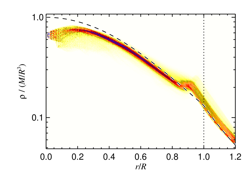
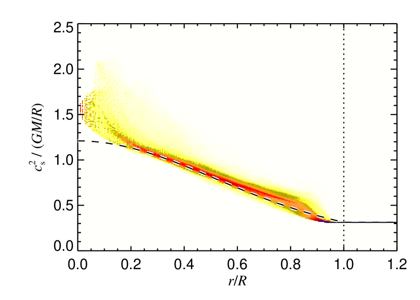
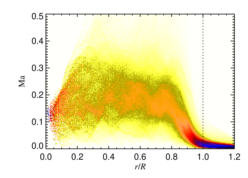
Figure 2.— “Histograms” of density $\varrho$, squared sound speed $c_{\rm s}^{2}$, Mach number $\mathrm{Ma}=|\mathbf{u}|/c_{\rm s}$, and specific entropy $s$ as a function of radius for the saturated state of Run 1c. Dark shades indicate a high probability of the corresponding value at a given radius. The dashed lines represent the initial profiles.

3.1. Radial stratification

Figure 2 shows density, squared sound speed (proportional to temperature), Mach number and specific entropy as function of radius for Run 1c. Density and squared sound speed vary by a factor of about $5$ from the center to the stellar surface. Apart from a few localized transients, the maximum Mach number is below unity and there is no evidence for shocks. The total variation in specific entropy is about $0.6\,c_{p}$. Even in the bulk of the convection zone ($0.15<r/R<0.85$) the specific entropy has a standard deviation of about $0.05\,c_{p}$, which is still much larger than what mixing-length theory predicts for this type of star. This is related to the high value of $\mathcal{L}$ that we are using, which is also the reason for the enhanced entropy values in the core. The location of the specific entropy minimum is at $r/R\approx 0.93$, i.e. somewhat below the nominal surface of the star. This is primarily a consequence of the rather large width of the profile functions for cooling and velocity damping, which affect the interior already inside $r=R$. At that effective radius, we naturally get a thin overshoot layer (as found in real stellar chromospheres).

3.2. Hydrodynamic flow patterns

Since the initial magnetic field is weak (several orders of magnitude below saturation), the kinematic phase of the dynamo represents the hydrodynamic flow pattern in a nonmagnetic scenario. Figure 3 shows an equatorial section of entropy and density for Run 1b. One can clearly distinguish narrow cool structures (downdrafts) that are familiar from box simulations of compressible convection (e.g. Hurlburt et al., 1986; Nordlund et al., 1992) The flows are far from being laminar, as can also be seen in the inset to Fig. 4. However, given the numerical resolution, only a limited range of scales can be resolved, as can be seen from the magnetic energy spectrum during the kinematic dynamo phase (see next section).

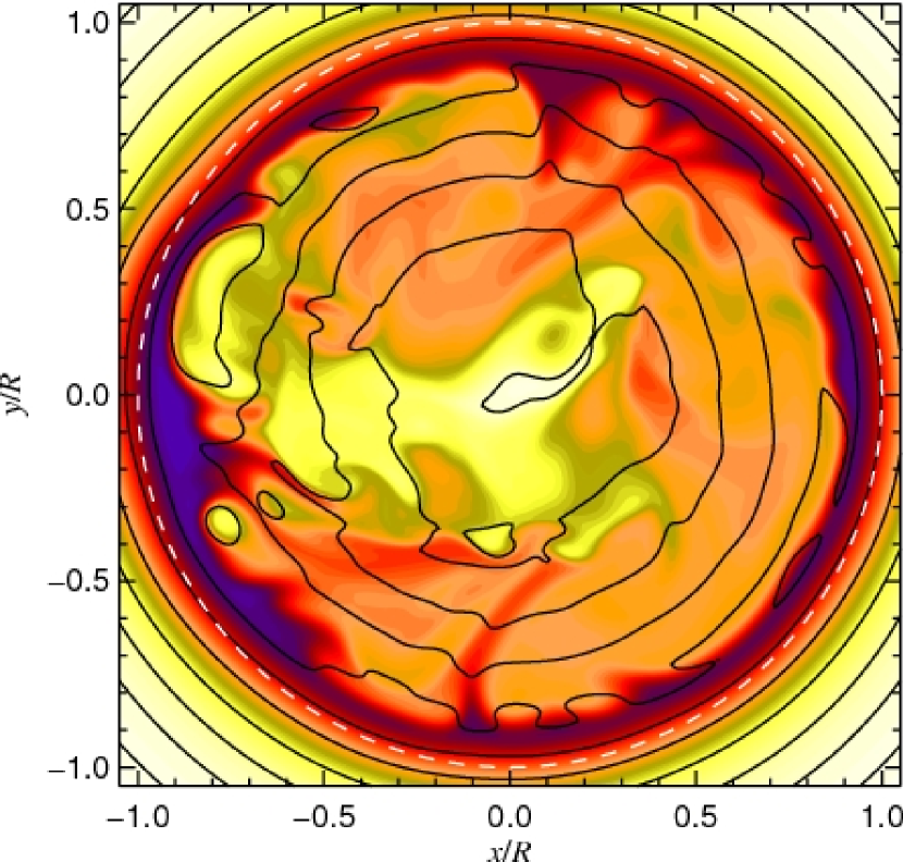
Figure 3.— Equatorial section of entropy (color coded: dark for low, bright for high entropy) and density (isolines) during the kinematic stage of Run 1b (at $t=300\,[t]$), where the magnetic field does not affect the dynamics.

Figure 5 shows a $t$-$\varphi$ average of kinetic helicity $\mathbf{u}\cdot\mbox{\boldmath{$\nabla$}}\times\mathbf{u}$ for the kinematic dynamo phase. As expected from the action of the Coriolis force on expanding upflows and contracting downflows, the helicity is predominantly negative in the northern and positive in the southern hemisphere. If kinetic helicity is connected to a turbulent electromotive force, we find a distribution of the $\alpha$ effect that is reminiscent of classical mean-field dynamo models (e.g. Roberts, 1972). It should hence not be surprising if the flow generates a large-scale magnetic field.

Figure 4.— Evolution of root-mean-square velocity $u_{\rm rms}$ and magnetic field $B_{\rm rms}$ (represented as an Alfvén speed using $\overline{\varrho}=0.4\,[\varrho]$ to make the two curves comparable) for Run 1b. Time is measured in units $[t]$ and velocities in units $[u]$ (see Sec. 2.4). The inset shows the maximum velocity $u_{\rm max}(t)$ during the onset of convection — note the irregular time-behavior.

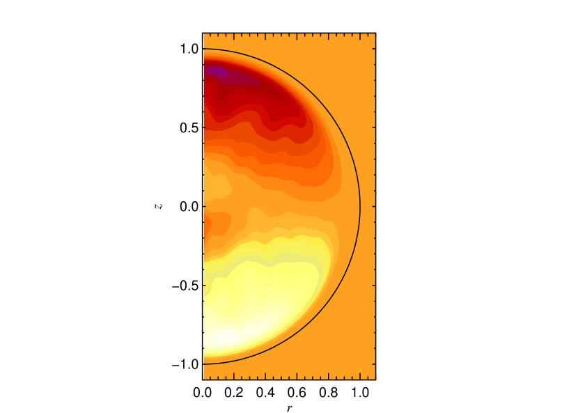
Figure 5.— Average of kinetic helicity for Run 2c during the kinematic phase. Shown is the azimuthal average of $\mathbf{u}\cdot\mbox{\boldmath{$\nabla$}}\times\mathbf{u}$, averaged in time from $t=100\mbox{--}300\,[t]$.

3.3. Dynamo action

The turbulent kinetic energy quickly reaches a statistically steady state after about 5 dynamical times ($t\approx 5\,[t]$), while the energy of the initially random magnetic field decays at first; see Fig. 4. This is because most of the magnetic energy of the random field is in the small scales and thus gets quickly dissipated. The magnetic field then grows exponentially with a growth rate $\lambda={\rm d}{}\ln B_{\rm rms}/{\rm d}{}t$ of about $0.04/[t]$ (for Run 1b).

Figure 6.— Spectra of the magnetic field for times $t=(300,600,900,1200,1500,2100)\,[t]$ of Run 2c (for this run, exponential field growth levels off around $t\approx 700\,[t]$). Magnetic energy increases with time and eventually reaches saturation. At late times the largest scales dominate.

Figure 7.— Magnetic (solid line) and kinetic (dashed line) power spectra for the saturated phase of Run 2c. While the velocity spectrum peaks around $k\approx 2\pi/R$, magnetic energy is distributed more flatly around the largest scales. For comparison, the dotted line shows the kinetic spectrum during the kinematic dynamo phase.

During the kinematic stage of the dynamo, the magnetic field grows exponentially with the same rate at all wavenumbers, so the spectrum remains shape-invariant, as can be seen in Fig. 6. The maximum of the magnetic spectrum is around $k\approx 3\times 2\pi/R$. The growth time $1/\lambda$ is about one order of magnitude shorter than the global diffusive time scale $\tau_{\rm Ohm}$, which is a manifestation of turbulent magnetic diffusion.

At later times, magnetic energy saturates first at the smallest scales, while the large scales still accumulate energy. Eventually all scales are saturated, but now the magnetic spectrum peaks at a larger scale than during the kinematic stage. As the magnetic field reaches saturation, the kinetic energy of the flow is decreased by a certain amount that depends on the relative importance of rotation (see Table 1). For slowly rotating spheres the kinetic energy decreases by only about 10–20% (Runs 1a and 2b), but for more rapidly rotating spheres, where the magnetic energy is also much larger, the suppression of the kinetic energy is about 50–60% (Runs 2c–2e). The strong dependence of the kinetic energy on the magnetic field strength suggests that the flows are probably not strongly turbulent and still governed by a large scale more laminar flow pattern.

Increasing the resolution by a factor of 2, while at the same time decreasing dissipative effects (cf. Runs 1a, 1b), we see that the growth rate increases significantly (by a factor of 2.5, see Table 1), but in the saturated state the rms velocity changes insignificantly. The rms magnetic field increases by about 40%, which is rather large and may be a consequence of the dynamo not being strongly supercritical. Decreasing the luminosity by a factor of 2 (cf. Runs 1b, 1c) decreases rms velocity and magnetic field only by about 20%.

Figure 7 shows spatial spectra of kinetic and magnetic energy. Kinetic energy peaks at a wavenumber of about $k_{\rm p}\approx 1\times 2\pi/R\approx 6\,[x]^{-1}$, which corresponds to the energy-carrying scale [smaller scales have a negligible contribution to the total kinetic energy $\int E(k){\rm d}{}k$]. The corresponding turnover time is $\tau=(u_{\rm rms}k_{\rm p})^{-1}\approx 2\,[t]$. This results in a normalized growth rate $\lambda\tau=0.08$, which is comparable to the values for both helically and nonhelically forced turbulence simulations where $\lambda\tau=0.03\mbox{--}0.1$, see Brandenburg (2001) and Haugen et al. (2004), respectively. The saturation value of magnetic energy is typically an order of magnitude below the kinetic energy of the turbulence for the slowly rotating models. This is quite similar to the ratio found in earlier simulations of convection driven dynamos in Cartesian and spherical geometries (Meneguzzi & Pouquet, 1989; Nordlund et al., 1992; Brun, 2004). For the faster rotating Runs 2c–2e, however, magnetic energy is comparable to kinetic energy.

Theoretically, there is always the possibility of different solutions to a nonlinear problem, depending on the initial conditions. This possibility has been anticipated in connection with the geodynamo (Roberts & Soward, 1992), but it has so far not been seen in any turbulent dynamo simulation (e.g. Glatzmaier & Roberts, 1995). In principle there is even the possibility of so-called self-killing dynamos that decay after full saturation has been reached, but such behavior has so far only been found under rather artificial conditions and in the absence of turbulence (Fuchs et al., 1999). In some cases we have restarted our simulations from a snapshot that has been obtained for different parameters. In such cases we always recovered statistically the same solution that was obtained in the standard way by starting from a weak seed magnetic field and a non-convecting initial state. This was further confirmed by restarting Run 2c with a $10^{10}$ times weaker initial field, which led to an indistinguishable time history of $u_{\rm max}$ for $t<5\,[t]$, and to statistically equivalent behavior for larger times.

The saturation appears to happen on a dynamical time scale, i.e. we see no evidence for resistively limited saturation, as it was found in helically forced simulations in a triply periodic domain (Brandenburg, 2001). In Run 1b, the total simulated time $t\approx 700\,[t]$ corresponds to about $2\,\tau_{\rm Ohm}$. The nonresistive saturation behavior could be due to the fact that in the present simulations the boundaries are open and permit a magnetic helicity flux across the equatorial plane and out of the box (Brandenburg & Dobler, 2001; Brandenburg, 2005). Another possibility is that the magnetic Reynolds number is still too small for magnetic helicity conservation to have an effect.

3.4. Dependence on rotation rate

In Runs 2a–2e, we vary the rotation rate $\Omega_{0}$, while keeping all other parameters fixed. As the rotation rate is increased, the root-mean-square velocity of the turbulence decreases. This is to be expected, because the presence of rotation is known to delay the onset of convection (e.g. Chandrasekhar, 1961). The rms magnetic field strength increases monotonically with the Coriolis number (or the rotation rate $\Omega_{0}$) for the runs shown.

In the absence of rotation (Run 2a), there is no net helicity or net shear and hence no reason for the generation of a large-scale magnetic field. However, we still find that the magnetic energy increases, albeit more slowly and to a lower value than for the rotating runs. This is a manifestation of the ‘fluctuating’ or ‘small-scale’ dynamo (Kazantsev, 1968; Meneguzzi et al., 1981; Cattaneo, 1999), which requires a considerably larger value of the magnetic Reynolds number than the helical dynamo, and there are indications that Run 2a is only mildly supercritical.

Figure 8.— Magnetic energy spectra for the saturated states of Runs 2a, 2b, 2c, 2d, and 2e.

Comparing the magnetic energy spectra for runs with different rotation rates (Fig. 8), we find that the magnetic energy at the large scales increases with $\Omega_{0}$ at least up to $\Omega_{0}\approx 5$ (corresponding to $\mbox{Co}\approx 100$), while the small scales are only weakly affected by rotation. The saturation for rapid rotation has been predicted by mean-field dynamo theory, (Rüdiger & Kichatinov, 1993; Ossendrijver et al., 2001), and for even larger $\Omega_{0}$, one expects a reduction of large-scale dynamo efficiency. However, for our models the peak dynamo efficiency occurs for rather large values of Co. Another surprise is that dynamo activity at small scales ($kR/2\pi\gtrsim 10$) is not quenched for ‘superfast’ rotation, although the Coriolis force should play a significant role until $k$ reaches significantly larger values.

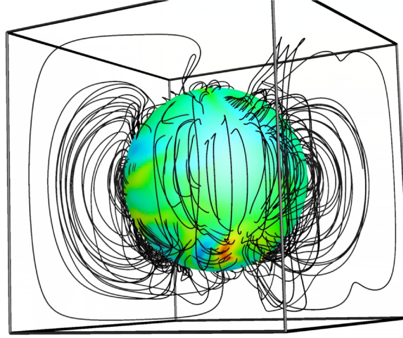
Figure 9.— Three-dimensional visualization of the magnetic field for Run 2c at $t=2600\,[t]$ (saturated phase). Magnetic field lines are shown, together with the surface of the sphere.

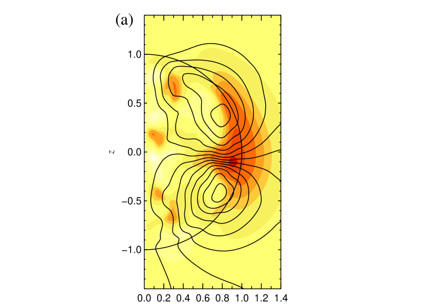
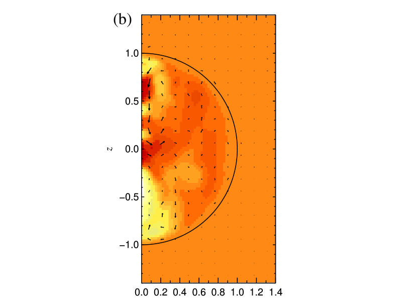
Figure 10.— Azimuthal averages of magnetic field (a) and velocity (b) for Run 2c at time $t=2100\,[t]$ (saturated phase). Panel (a) shows poloidal field lines of the $\varphi$-averaged magnetic field (orientation of the field lines in the top half is predominantly counter-clockwise), superimposed on a color/gray-scale representation of the azimuthal mean field, $\overline{B_{\varphi}}$, with bright colors representing $\overline{B_{\varphi}}>0$ and dark colors representing $\overline{B_{\varphi}}<0$. Note the mixed parity of the structure of the mean field with a strong quadrupolar contribution. Panel (b) shows vectors of the mean poloidal velocity superimposed on a color/gray scale representation of the mean angular velocity $\delta\overline{\Omega}(r,z)\equiv\overline{u_{\varphi}}/(r\sin\theta)$ with bright colors for $\delta\overline{\Omega}>0$ and dark colors for $\delta\overline{\Omega}<0$. Note that for different snapshots in time the velocity field $\overline{\mathbf{u}}$ looks very different.

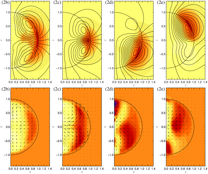
Figure 11.— Azimuthal averages for Runs 2b–2e as in Fig. 10, but now the fields are additionally averaged over $1000$–$2000$ time units [$t$] (about $150$–$300$ turbulent turnover times, or $4$–$8$ $\tau_{\rm Ohm}$) during the saturated state. Angular velocity $\Omega_{0}$ increases from left to right; the panels are labeled by the names of the individual runs. Top row: magnetic field. Orientation of the field lines is predominantly counterclockwise in the top hemisphere and clockwise in the bottom hemisphere in all four panels. Bottom row: velocity. Note that the angular velocity shows some tendency to be constant along cylinders for Runs 2b and 2c, while magnetic and velocity field are asymmetric for Runs 2d and 2e. The amplitudes of magnetic and velocity fields have been scaled individually for each image; absolute values of $B_{\rm rms}$ and $u_{\rm rms}$ are given in Table 1.

3.5. Large-scale field structure

Although a lot of the magnetic energy is due to the small-scale structures, as can be seen in the magnetic energy spectra, outside the star the field shows features of a dipole-like structure with a noticeable contribution from the first few multipoles; see Fig. 9 where we show a visualization of the three-dimensional magnetic field lines.

A more quantitative presentation of the large-scale magnetic and velocity fields is obtained by considering azimuthal averages, as shown in Fig. 10 for one snapshot of Run 2c. The magnetic field shows a clear large-scale component with predominantly quadrupolar symmetry with respect to the midplane, but still including dipolar contributions. The velocity field shows little large-scale structure and varies strongly in time.

We find a considerably more regular structure when applying time averaging to the azimuthally averaged data. In Fig. 11 we show, for the saturated states, the correspondingly averaged magnetic fields (top row) and velocity fields (bottom row) for four different runs with rotation rate $\Omega_{0}$ increasing from left to right. We note that for all runs the averaged velocity field changes very little from the kinematic to the saturated stage of the dynamo.

Table 2Additional diagnostic quantities for Runs 2a–2e.

Run	$\Omega_{0}$	$q_{\mathbf{u}}$	$q_{\mathbf{B}}$	$p_{\mathbf{u}}$	$p_{\mathbf{B}}$	$\Delta\omega^{\rm kin\,/\,sat}$	$\sigma_{\mathbf{u}}^{\rm kin\,/\,sat}$	$\sigma_{\mathbf{B}}^{\rm kin\,/\,sat}$	$P$
2a	$0.0$	$0.30$	$0.02$	$0.04$	$1.10$	$0.53$ / $0.24$	$0.240$ / $0.214$	$0.071$ / $0.079$	$-0.12$
2b	$0.5$	$0.38$	$0.19$	$1.44$	$2.95$	$1.23$ / $0.97$	$0.222$ / $0.221$	$0.077$ / $0.147$	$+0.99$
2c	$2.0$	$0.14$	$0.39$	$1.80$	$2.36$	$0.56$ / $0.22$	$0.062$ / $0.079$	$0.124$ / $0.271$	$+0.91$
2d	$5.0$	$0.14$	$0.40$	$1.59$	$1.32$	$0.82$ / $0.26$	$0.054$ / $0.064$	$0.046$ / $0.271$	$+0.28$
2e	$10.0$	$0.14$	$0.46$	$1.27$	$1.17$	$0.50$/ $\,0.14$	$0.080$ / $0.063$	$0.047$ / $0.326$	$-0.28$

Note. — All quantities refer to the saturated state, unless explicitly labeled with ‘kin’.

With this averaging, we find almost perfect quadrupolar symmetry for $\mathbf{B}$ in Runs 2b and (slightly less pronounced) 2c. On the other hand, Runs 2d and 2e show very pronounced hemispheric asymmetry that appears to be relatively long-lived. For Runs 2b and 2c, the velocity field shows a meridional circulation pattern that is directed outwards at the equator, and surfaces of constant angular velocity $\omega$ are approximately cylindrical. For the rapidly spinning Runs 2d and 2e, the asymmetry in the magnetic structure is reflected in differential rotation and meridional circulation.

An explicit measure for the efficiency of large-scale field generation is the ratio

$$q_{\mathbf{B}}\equiv\frac{\bigl{<}\bigl{<}\overline{\mathbf{B}}\bigr{>}_{t}^{\,2}\bigr{>}_{rz}^{\,1/2}}{B_{\rm rms}}\;,$$ (15)

which is given in Table 2. A similar quantity $q_{\mathbf{u}}$ is also defined for the velocity. Here the overbar denotes azimuthal averaging, $\left<\cdot\right>_{t}$ represents time averaging, while $\left<\cdot\right>_{rz}$ denotes spatial averaging over the sphere, and $B_{\rm rms}=\langle\langle\overline{\mathbf{B}^{2}}\rangle_{t}\rangle_{rz}$. This ratio is $q_{\mathbf{B}}=0.19$ for Run 2b and increases further with the rotation rate. These values are quite large, suggesting that large-scale field generation is quite efficient. However, in forced turbulence simulations with open boundaries and no shear (Brandenburg & Dobler, 2001), $q_{\mathbf{B}}$ decreases with increasing magnetic Reynolds number. On the other hand, simulations of forced turbulence suggest that the presence of shear is critical for allowing the dynamo amplitude to be independent of the magnetic Reynolds number (Brandenburg, 2005). Further numerical simulations are necessary to see whether the same behavior occurs here as well.

The ratios

$$p_{\mathbf{u}}\equiv\frac{\bigl{<}\bigl{<}\overline{u_{\varphi}}\bigr{>}_{t}^{\,2}\bigr{>}_{rz}^{\,1/2}}{\bigl{<}\bigl{<}\overline{u_{\rm pol}}\bigr{>}_{t}^{\,2}\bigr{>}_{rz}^{\,1/2}}\;,\qquad p_{\mathbf{B}}\equiv\frac{\bigl{<}\bigl{<}\overline{B_{\varphi}}\bigr{>}_{t}^{\,2}\bigr{>}_{rz}^{\,1/2}}{\bigl{<}\bigl{<}\overline{B_{\rm pol}}\bigr{>}_{t}^{\,2}\bigr{>}_{rz}^{\,1/2}}$$ (16)

quantify the importance of the azimuthal components in the $\varphi$- and $t$-averaged fields. In the non-rotating case, $p_{\mathbf{u}}$ is very small, indicating that systematic azimuthal flows are weak. With increasing angular velocity, however, $p_{\mathbf{u}}$ at first increases as systematic differential rotation evolves. The slight decline of $p_{\mathbf{u}}$ in Runs 2d and 2e is connected with the stronger magnetic field in those cases. In fact, both the azimuthal component $\langle\langle\overline{u_{\varphi}}\rangle_{t}^{\,2}\rangle_{rz}^{\,1/2}$ and the poloidal component $\langle\langle\overline{u_{\rm pol}}\rangle_{t}^{\,2}\rangle_{rz}^{\,1/2}$ decrease monotonically from Runs 2b to 2e because of the increasing large-scale magnetic field.

The ratio $p_{\mathbf{B}}$ is 1.1 in the nonrotating case, it has a maximum already for $\Omega_{0}=0.5$ (Run 2b) and then declines. The total magnetic energy continues to grow with higher rotation rates (see Table 1), indicating that with increasing rotation rate the poloidal field continues to grow, while the toroidal field remains roughly unchanged. This seems to be in qualitative agreement with the simulations by Brun et al. (2004) for dynamos in convective shells without tachocline. On the other hand, this ratio is in all cases small compared to what is expected for the Sun, where the tachocline can be expected to have a strong effect.

With the exception of Run 2b, the absolute amplitude $\Delta\omega$ of the differential rotation for kinematic and saturated states is similar. This is consistent both with theory (Kitchatinov & Rüdiger, 1999) and with observations showing only a weak dependence of surface differential rotation on stellar rotation for late type stars (Barnes et al., 2005), which are however not fully convective.

Next, we show the energy ratios

$$\sigma_{\mathbf{u}}\equiv\frac{\langle\langle\overline{\mathbf{u}}^{2}\rangle_{t}\rangle_{rz}}{u_{\rm rms}^{2}}\;,\qquad\sigma_{\mathbf{B}}\equiv\frac{\langle\langle\overline{\mathbf{B}}^{2}\rangle_{t}\rangle_{rz}}{B_{\rm rms}^{2}}\;,$$ (17)

quantifying the fraction of energy contained in the axisymmetric part of $\mathbf{u}$ and $\mathbf{B}$. For most of the rotating runs, $\sigma_{\mathbf{B}}$ increases drastically from the kinematic stage to saturation. This is another manifestation of the trend towards large-scale fields once the small scales are saturated (see Fig. 6). On the other hand, $\sigma_{\mathbf{u}}$, which is strongly reduced by rotation, is not severely affected by the magnetic field saturation.

Finally, we consider the parity of the mean field with respect to the equatorial plane. Earlier work on mean-field dynamos in full spheres (Brandenburg et al., 1989) has shown that for weakly supercritical dynamos the parity is dipolar (antisymmetry with respect to the equator). However, as the dynamo becomes more supercritical, the parity can become quadrupolar (symmetric with respect to the equator), but mixed and chaotic behaviors are also possible (Covas et al., 1999). Parity of the mean field can be quantified as

$$P=\frac{E_{\rm S}-E_{\rm A}}{E_{\rm S}+E_{\rm A}}\;,$$ (18)

where $E_{\rm S}$ and $E_{\rm A}$ denote the energies contained in the symmetric and antisymmetric parts of $\overline{\mathbf{B}}$. The values of $P$ are listed in Table 2 for the saturated stage of the dynamo. For Runs 2b and 2c the mean field is nearly quadrupolar $P\approx+1$, as is also evident from Fig. 11. Both in the absence of rotation and for strong rotation the mean fields are of more mixed parity character. Comparison with mean-field dynamos would suggest that our Runs 2b and 2c are in the “more supercritical” regime. However, we have not found a case that would clearly belong to the weakly supercritical regime, where dipolar fields are expected. In addition, mean-field theory would suggest cyclic mean fields, that have also not been seen. It is possible that such features would emerge in a direct simulation only after many more turnover times than what has been possible here.

The ratios $q$ and $p$ allow us primarily to assess the mode of operation of the dynamo found in the simulations. In particular, they provide a sensitive tool to assess the possible dependence of the magnitude of large-scale fields on the magnetic Reynolds number. Observationally, of course, only the limit of very large magnetic Reynolds numbers is relevant. More detailed comparison of the $q$ and $p$ ratios with observations is hampered by the fact that the magnetic field in the star’s interior cannot be measured with current techniques. The interpretation of proxies such as filling factors and the appearance of magnetic fields at the stellar surface may be premature as long as we do not fully understand the connection between magnetic fields at the surface and the interior. For example, the interpretation of bipolar spots in terms of distinct flux tubes may not be valid and hence the presence of spots may not necessarily indicate a high degree of intermittency in the interior (Brandenburg, 2005). However, once the physics of the stellar surface is modeled more realistically (e.g., without imposing an artificial cooling layer to model radiation) it would be useful to produce synthetic surface maps and light curves that can be compared with observations.

4. Conclusions

The present work suggests that fully convective stars are capable of generating not only turbulent magnetic fields, but also strong large-scale fields that dominate the magnetic energy spectrum. In most of our models, the large-scale field has a strong quadrupolar component, in contrast to what is expected from mean-field theory for dynamo action in thick shells and in full spheres (Roberts, 1972). We have so far not seen evidence of magnetic cycles. The resolution of our models is still too low to be able to tell whether this type of magnetic field generation will continue to operate at much larger magnetic Reynolds numbers, but our results disprove the claim that a strong shear layer or a stably stratified core are necessary ingredients for the generation of large-scale magnetic fields. As one would expect in the absence of strong shear layers, the toroidal and poloidal components of the mean magnetic field are roughly comparable.

Another important result concerns the self-consistently produced differential rotation. In our simulations, the angular velocity shows some tendency to be constant along cylinders, which is plausible for rapidly rotating stars. Whether or not this is realistic is difficult to say. Asteroseismology may in the future be able to reveal the internal angular velocity of stars, but at present the time coverage is still too short and incomplete. There is at least some hope of observing the surface differential rotation, at least of sufficiently rapidly rotating fully convective stars such as T Tauri stars, using surface imaging (Collier Cameron et al., 2004). This would be particularly interesting, given that our simulations predict a more slowly rotating equator. This behavior is opposite to that in the solar case. Thus far, theory in terms of the $\Lambda$ effect (e.g. Rüdiger & Hollerbach, 2004) also tends to produce a faster equator, unless the turbulent motions possess a predominantly radial structure ($u_{r,{\rm rms}}\gg u_{\varphi,{\rm rms}}$). In our case, however, there is strong meridional circulation, which, due to conservation of angular momentum, causes the outer layers to rotate more slowly; see Kitchatinov & Rüdiger (2004). Again, this result may no longer hold in real stars, because in our model the degree of stratification is far too low and the luminosity too high, so the convective velocities and meridional circulation tend to be exaggerated.

Another reason for the slowly rotating equator could be connected with the outer boundary condition. In connection with geodynamo simulations there are indications that a no-slip outer boundary condition (with respect to a rigidly rotating sphere) tends to produce a more slowly rotating equator (Christensen et al., 1999). In the limit of a short damping time, our effective outer boundary condition at $r=R$ should indeed be closer to a no-slip condition than to a free-slip condition. On the other hand, in strongly magnetized stars the coronal magnetic field may enforce a rigidly rotating exterior, and hence produce conditions close to what is represented by our model.

Appendix A Reference model

In order to specify the initial conditions and the gravity potential, we use a simple spherically symmetric, hydrostatic, self-gravitating, isentropic model. The equations for this reference model are

$$\frac{dm_{r}}{dr} = 4\pi r^{2}\varrho\;,$$ (A1)

$$\frac{d\varrho}{dr} = -\frac{G\,m_{r}\varrho^{2-\gamma}}{\gamma Kr^{2}}\;,$$ (A2)

where $m_{r}$ denotes the total mass inside the sphere of radius $r$, together with the boundary conditions

$$m_{r}(0)=0\;,\qquad\varrho(0)=\varrho_{\rm c}\;.$$ (A3)

Here $K=e^{\gamma s_{0}/c_{p}}=\mathrm{const}$ is the polytropic constant, relating pressure $p$ and density $\varrho$ via $p=K\varrho^{\gamma}$, and $s_{0}$ is the constant value of entropy. The adiabatic exponent is $\gamma=5/3$, and thus our reference model is a polytropic model with polytropic index $m=3/2$.

Equations (A1) and (A2) are integrated outwards, starting with certain values $(\varrho_{\rm c},s_{0})$ for central density and entropy. As is common with polytropic models, the solution can have a surface (where $\varrho=p=T=0$) at some finite radius $R_{\rm surf}$, which must not be smaller than the desired stellar radius $R$.

Varying the central values $(\varrho_{\rm c},s_{0})$, we can tune the reference model to match a given reference stellar radius $R$ and total mass $M$. We choose the values $R=0.27\,R_{\odot}=1.9\times 10^{8}\,\mathrm{m}$, and $M=0.21\,M_{\odot}=4.2\times 10^{29}\,\mathrm{kg}$, which correspond to an M5 dwarf with a luminosity of $L=0.008\,L_{\odot}=3\times 10^{24}\,\mathrm{W}$.

Once the temperature and density profiles are known, one can calculate the approximate volume heating rate according to the formula

$$\mathcal{H}(\varrho,T)\approx 4.9\times 10^{-4}\left(\frac{\varrho}{10^{5}\,\mathrm{kg\,m^{-3}}}\right)^{2}\left(\frac{T}{10^{6}\,\mathrm{K}}\right)^{5.3}{\rm W\,m^{-3}}\;.$$ (A4)

The $T^{5.3}$ dependence is an approximation for the $pp1$ chain of hydrogen burning near $T_{\rm c}\approx 6\times 10^{6}\,\mathrm{K}$; see Sec. 18.5.1 of Kippenhahn & Weigert (1990). We have used a Gaussian approximation to this (time-independent) radial dependence of $\mathcal{H}(r)$ for all simulations presented here, while adjusting the total luminosity by a multiplicative factor. Figure 1 shows the luminosity $L_{r}(r)$ as a function of radius.

Appendix B High-order upwind derivatives

Convection simulations with high-order centered finite-difference schemes sometimes show a tendency to develop ‘wiggles’ (Nyquist zigzag) in $\ln\varrho$. This can be avoided by using a high-order upwind derivative operator, where the point furthest downstream is excluded from the stencil. We apply this technique only to the terms $\mathbf{u}\cdot\mbox{\boldmath{$\nabla$}}\ln\varrho$ and $\mathbf{u}\cdot\mbox{\boldmath{$\nabla$}}s$. In the following we discuss the treatment in the $x$ direction, but the treatment for the other directions is analogous. For $u_{x}>0$, we replace

$$D_{\rm cent,6}\,f_{0}=\frac{-f_{-3}+9f_{-2}-45f_{-1}+45f_{1}-9f_{2}+f_{3}}{60\,\delta x}=f^{\prime}_{0}+\frac{\delta x^{6}\,f^{(7)}(\xi_{6})}{140}\;,\qquad x_{-3}<\xi_{6}<x_{3}\;,$$ (B1)

by

$$D_{\rm up,5}\,f_{0}=\frac{-2f_{-3}+15f_{-2}-60f_{-1}+20f_{0}+30f_{1}-3f_{2}}{60\,\delta x}=f^{\prime}_{0}-\frac{\delta x^{5}\,f^{(6)}(\xi_{5})}{60}\;,\qquad x_{-3}<\xi_{5}<x_{2}\;.$$ (B2)

Both formulæ follow from Markoff’s formula (Abramowitz & Stegun, 1984, §25.3.7).

The difference between the sixth-order central and fifth-order upwind derivative is proportional to the sixth derivative operator

$$D^{6}_{\rm cent,2}\,f_{0}=\frac{f_{-3}-6f_{-2}+15f_{-1}-20f_{0}+15f_{1}-6f_{2}+f_{3}}{\delta x^{6}}=f^{(6)}_{0}+\frac{\delta x^{2}f^{(8)}(x_{0})}{4}+O(\delta x^{4})\;,$$ (B3)

namely

$$D_{\rm up,5}\,f_{0}=D_{\rm cent,6}\,f_{0}-\alpha\,\delta x^{5}D^{6}_{\rm cent,2}\;,$$ (B4)

with $\alpha=1/60$. This allows us to represent the fifth-order upwind scheme in the advection term (for both signs of $u_{x}$) by sixth-order hyper-diffusion:

$$-u_{x}f^{\prime}_{\rm up,5}=-u_{x}f^{\prime}_{\rm cent,6}+\alpha|u_{x}|\,\delta x^{5}f^{(6)}_{\rm cent,2}\;.$$ (B5)

References

- Abramowitz & Stegun (1984) Abramowitz, M., & Stegun, I. A. 1984, Pocketbook of Mathematical Functions (Thun, Frankfurt: Harri Deutsch)
- Barnes et al. (2005) Barnes, J. R., Collier Cameron, A., Donati, J.-F., James, D. J., Marsden, S. C., & Petit, P. 2005, MNRAS, 357, L1
- Barnes et al. (2004) Barnes, J. R., James, D. J., & Collier Cameron, A. 2004, MNRAS, 352, 589
- Berger et al. (2005) Berger, E. et al. 2005, ApJ, 627, 960
- Brandenburg (2001) Brandenburg, A. 2001, ApJ, 550, 824
- Brandenburg (2005) —. 2005, ApJ, 625, 539
- Brandenburg et al. (2005) Brandenburg, A., Chan, K. L., Nordlund, Å., & Stein, R. F. 2005, AN, 326, 681
- Brandenburg & Dobler (2001) Brandenburg, A., & Dobler, W. 2001, A&A, 369, 329
- Brandenburg et al. (1989) Brandenburg, A., Tuominen, I., Krause, F., Meinel, R., & Moss, D. 1989, A&A, 213, 411
- Browning et al. (2004) Browning, M. K., Brun, A. S., & Toomre, J. 2004, ApJ, 601, 512
- Brun (2004) Brun, A. S. 2004, SoPh, 220, 333
- Brun et al. (2005) Brun, A. S., Browning, M. K., J., & Toomre. 2005, ApJ, 629, 461
- Brun et al. (2004) Brun, A. S., Miesch, M. S., & Toomre, J. 2004, ApJ, 614, 1073
- Brun & Toomre (2002) Brun, A. S., & Toomre, J. 2002, ApJ, 570, 865
- Cattaneo (1999) Cattaneo, F. 1999, ApJ, 515, L39
- Chan & Sofia (1986) Chan, K. L., & Sofia, S. 1986, ApJ, 307, 222
- Chandrasekhar (1961) Chandrasekhar, S. 1961, Hydrodynamic and Hydromagnetic Stability (Oxford: Clarendon)
- Christensen et al. (1999) Christensen, U., Olson, P., & Glatzmaier, G. A. 1999, Geophys. J. Int., 138, 393
- Collier Cameron et al. (2004) Collier Cameron, A., Schwope, A., & Vrielmann, S. 2004, AN, 325, 179
- Covas et al. (1999) Covas, E., Tavakol, R., Tworkowski, A., Brandenburg, A., Brooke, J., & Moss, D. 1999, A&A, 345, 669
- Dorch (2004) Dorch, S. B. F. 2004, A&A, 423, 1101
- Dorch & Ludwig (2002) Dorch, S. B. F., & Ludwig, H.-G. 2002, AN, 323, 402
- Durney et al. (1993) Durney, B. R., DeYoung, D. S., & Roxburgh, I. W. 1993, SoPh, 145, 207
- Freytag et al. (2002) Freytag, B., Steffen, M., & Dorch, B. 2002, AN, 323, 213
- Fuchs et al. (1999) Fuchs, H., Rädler, K.-H., & Rheinhardt, M. 1999, AN, 320, 129
- Gilman (1983) Gilman, P. A. 1983, ApJS, 53, 243
- Gizis et al. (2000) Gizis, J. E., Monet, D. G., Reid, I. N., Kirkpatrick, J. D., Liebert, J., & Williams, R. J. 2000, AJ, 120, 1085
- Glatzmaier (1985) Glatzmaier, G. A. 1985, ApJ, 291, 300
- Glatzmaier & Roberts (1995) Glatzmaier, G. A., & Roberts, P. H. 1995, Nature, 377, 203
- Haugen et al. (2004) Haugen, N. E. L., Brandenburg, A., & Dobler, W. 2004, PRE, 70, 016308
- Hawley (1993) Hawley, S. L. 1993, PASP, 105, 955
- Hawley et al. (2000) Hawley, S. L., Reid, I. N., & Gizis, J. 2000, in ASP Conference Series, Vol. 212, From Giant Planets to Cool Stars, ed. C. A. Griffith & M. S. Marley, 252–261
- Hawley et al. (1999) Hawley, S. L., Reid, I. N., Gizis, J. E., & Byrne, P. B. 1999, in Solar and Stellar Activity: Similarities and Differences, ed. C. J. Butler & J. G. Doyle, ASP Conf. Ser. No. 158, 63–74
- Hurlburt et al. (1986) Hurlburt, N. E., Toomre, J., & Massaguer, J. M. 1986, ApJ, 311, 563
- Johns-Krull et al. (1999a) Johns-Krull, C. M., Valenti, J. A., Hatzes, A. P., & Kanaan, A. 1999a, ApJ, 510, L41
- Johns-Krull et al. (1999b) Johns-Krull, C. M., Valenti, J. A., & Koresko, C. 1999b, ApJ, 516, 900
- Joncourt et al. (1994) Joncourt, I., Bertout, C., & Ménard, F. 1994, A&A, 285, L25
- Kazantsev (1968) Kazantsev, A. P. 1968, Zh. Eksp. Teor. Fiz., 26, 1031
- Kippenhahn & Weigert (1990) Kippenhahn, R., & Weigert, A. 1990, Stellar Structrue and Evolution, 1st edn. (Berlin & New York: Springer)
- Kitchatinov & Rüdiger (1999) Kitchatinov, L. L., & Rüdiger, G. 1999, A&A, 344, 911
- Kitchatinov & Rüdiger (2004) —. 2004, AN, 325, 496
- Kitchatinov et al. (1994) Kitchatinov, L. L., Rüdiger, G., & Küker, M. 1994, A&A, 292, 125
- Küker & Rüdiger (1997) Küker, M., & Rüdiger, G. 1997, A&A, 328, 253
- Küker & Rüdiger (1999) —. 1999, A&A, 346, 922
- Küker et al. (1993) Küker, M., Rüdiger, G., & Kitchatinov, L. L. 1993, A&A, 279, L1
- Meneguzzi et al. (1981) Meneguzzi, M., Frisch, U., & Pouquet, A. 1981, PRL, 47, 1060
- Meneguzzi & Pouquet (1989) Meneguzzi, M., & Pouquet, A. 1989, JFM, 205, 297
- Miesch et al. (2000) Miesch, M. S., Elliott, J. R., Toomre, J., Clune, T. L., Glatzmaier, G. A., & Gilman, P. A. 2000, ApJ, 532, 593
- Mohanty & Basri (2003) Mohanty, S., & Basri, G. 2003, ApJ, 583, 451
- Moreno-Insertis (1983) Moreno-Insertis, F. 1983, A&A, 122, 241
- Nordlund et al. (1992) Nordlund, Å., Brandenburg, A., Jennings, R. L., Rieutord, M., Ruokolainen, J., Stein, R. F., & Tuominen, I. 1992, ApJ, 392, 647
- Ossendrijver et al. (2001) Ossendrijver, M., Stix, M., & Brandenburg, A. 2001, A&A, 376, 713
- Porter et al. (2000) Porter, D. H., Woodward, P. R., & Jacobs, M. L. 2000, Ann. N.Y. Acad. Sci., 898, 1
- Roberts (1972) Roberts, P. H. 1972, Philos. Trans. R. Soc. London, A272, 663
- Roberts & Soward (1992) Roberts, P. H., & Soward, A. M. 1992, Annu. Rev. Fluid Dyn., 24, 459
- Rüdiger & Hollerbach (2004) Rüdiger, G., & Hollerbach, R. 2004, The Magnetic Universe: Geophysical and Astrophysical Dynamo Theory (Weinheim: Wiley-VCH)
- Rüdiger & Kichatinov (1993) Rüdiger, G., & Kichatinov, L. L. 1993, A&A, 269, 581
- Vilhu (1984) Vilhu, O. 1984, A&A, 133, 117
- Vilhu et al. (1989) Vilhu, O., Ambruster, C. W., Neff, J. E., Linsky, J. L., Brandenburg, A., Ilyin, I. V., & Shakhovskaya, N. I. 1989, A&A, 222, 179
- Weber et al. (2005) Weber, M., Strassmeier, K. G., & Washuettl, A. 2005, AN, 326, 287
- Woodward et al. (2003) Woodward, P. R., Porter, D. H., & Jacobs, M. 2003, in ASP Conference Series, Vol. 293, 3D Stellar Evolution, ed. S. Turcotte, S. C. Keller, & R. M. Cavallo, 45–63