Investigating The Possible Anomaly Between Nebular and Stellar
Oxygen Abundances in the Dwarf Irregular Galaxy WLM 

Abstract

We obtained new optical spectra of 13 H II regions in WLM with EFOSC2; oxygen abundances are derived for nine H II regions. The temperature-sensitive [O III]$\lambda 4363$ emission line was measured in two bright H II regions HM 7 and HM 9. The direct oxygen abundances for HM 7 and HM 9 are 12$+$log(O/H) = $7.72\pm 0.04$ and $7.91\pm 0.04$, respectively. We adopt a mean oxygen abundance of 12$+$log(O/H) = $7.83\pm 0.06$. This corresponds to [O/H] = $-0.83$ dex, or 15% of the solar value. In H II regions where [O III]$\lambda 4363$ was not measured, oxygen abundances derived with bright-line methods are in general agreement with direct values of the oxygen abundance to an accuracy of about 0.2 dex. In general, the present measurements show that the H II region oxygen abundances agree with previous values in the literature. The nebular oxygen abundances are marginally consistent with the mean stellar magnesium abundance ([Mg/H] = $-0.62$). However, there is still a 0.62 dex discrepancy in oxygen abundance between the nebular result and the A-type supergiant star WLM 15 ([O/H] = $-0.21$). Non-zero reddening values derived from Balmer line ratios were found in H II regions near a second H I peak. There may be a connection between the location of the second H I peak, regions of higher extinction, and the position of WLM 15 on the eastern side of the galaxy.

1. Introduction

Dwarf galaxies are thought to be the building blocks in the assembly of more massive galaxies within the hierarchical picture of structure formation. These galaxies are also very important venues in which questions about cosmology, galaxy evolution, and star formation may be answered. Dwarf irregular galaxies are relatively low-mass, gas-rich, metal-poor, and are presently forming stars as shown by their H II regions, whereas low-mass dwarf spheroidal galaxies are gas-poor and no longer host present-day star-forming events. The properties of these galaxies may be similar to those found in the early universe, and dwarf irregulars may possibly be sites out of which damped Lyman-$\alpha$ absorber systems form at high redshift (e.g., Calura et al., 2003; Prochaska et al., 2003). An important question which has yet to be fully explained is the relationship between dwarf irregular and dwarf spheroidal galaxies (e.g., Grebel et al., 2003; Skillman et al., 2003a, b; van Zee et al., 2004, and references therein). That streams have been observed within the Galaxy and M 31 (e.g., Yanny et al., 2003; Martin et al., 2004; Zucker et al., 2004a, b) has been taken as evidence of ongoing accretion and of representing past merging of dwarfs by the more massive galaxies. However, work presented by Tolstoy et al. (2003) and Venn et al. (2004a) have shown that stars in present-day dwarf spheroidals cannot make up the dominant stellar populations in the halo, bulge, or the thick disk of the Galaxy, although the merging of dwarf galaxies at very early times cannot be ruled out.

The measurements of element abundances provide important clues to understanding the chemical history and evolution of galaxies. In star-forming dwarf galaxies, the analysis of bright nebular emission lines from the spectra of H II regions is used to derive abundances of $\alpha$-elements (i.e., oxygen) in the ionized gas (see e.g., Dinerstein, 1990; Skillman, 1998; Garnett, 2004). However, a limited number of elements can be studied by comparison to the number of elements found in the absorption spectra of stars. For a more complete picture, additional elements should be included, since various elements arise from different sites and involve different timescales. Oxygen and other $\alpha$-elements are created in very massive progenitor stars before being returned to the interstellar medium (ISM) on short timescales, when these stars explode as Type II supernovae. Iron is an element produced by explosive nucleosynthesis in Type I supernovae from low-mass progenitor stars on longer timescales, and is also produced in Type II supernovae. Because of the varying timescales for stars of different masses, the $\alpha$ element-to-iron abundance ratio, [$\alpha$/Fe], is tied very strongly with the star formation history (e.g., Gilmore & Wyse, 1991; Matteucci, 2003). Interestingly, [$\alpha$/Fe] values for three dwarf irregular galaxies are near or at solar, which indicates that stars have been forming at a very low rate and/or the last burst of star formation occurred long ago (Venn et al., 2001, 2003; Kaufer et al., 2004). Izotov & Thuan (1999) claim that O/Fe is elevated in low metallicity blue compact dwarf galaxies ([O/Fe] = $+0.32\pm 0.11$). However, their analysis does not account for potential depletion of Fe onto dust grains, and the Fe abundance is only measured in Fe⁺², requiring very large and uncertain ionization correction factors (ICFs). Rodríguez (2003) finds that the adopted ICFs underestimate the total Fe abundance by factors larger than the elevated abundance ratio claimed by Izotov & Thuan (1999). Thus, it is prudent to assume that the nebular Fe abundances in these galaxies, and thus the nebular O/Fe ratios, are quite uncertain (Garnett, 2004). At present, reliable O/Fe ratios will need to be obtained from stellar abundances. While a complete discussion of $\alpha$/Fe values is beyond the scope of the present work, brief reviews of stellar abundances in external galaxies have recently been presented by Tolstoy & Venn (2004) and Venn et al. (2004b).

High efficiency spectrographs on 8- and 10-m telescopes have made possible the spectroscopic measurements of individual stars in extragalactic systems. In particular, bright blue supergiants have been observed in galaxies at distances of about 1 Mpc. These hot young massive stars allow us to measure simultaneously present-day $\alpha$- and iron-group elements. The important advantage of these measurements also allow for the direct comparison of stellar $\alpha$-element abundances with nebular measurements, as massive stars and nebulae are similar in age and have similar formation sites. Oxygen abundances derived from the spectroscopy of blue supergiants have been obtained in nearby dwarf irregular galaxies NGC 6822, WLM, and Sextans A (Venn et al., 2001, 2003; Kaufer et al., 2004).

The relative ease with which spectra of H II regions have been obtained in dwarf irregular galaxies has led to establishing: (1) the metallicity-luminosity relation, thought to be representative of a mass-metallicity relation for dwarf irregular galaxies (e.g., Skillman et al., 1989a; Richer & McCall, 1995; Lee et al., 2003b); and (2) the metallicity-gas fraction relation, which represents the relative conversion of gas into stars, and may be strongly affected by the galaxies’ surrounding environment (e.g., Lee et al., 2003b, c; Skillman et al., 2003a). It is assumed that nebular oxygen abundances are representative of the present-day ISM metallicity for an entire dwarf galaxy, where there is often only a single H II region present. In fact, spatial inhomogeneities or radial gradients in oxygen abundances have been found to be very small or negligible in nearby dwarf irregular galaxies (e.g., Kobulnicky & Skillman, 1996, 1997), although recent observations have cast uncertainty about the assumption in NGC 6822 and WLM (Venn et al., 2001, 2003). Here we will focus on oxygen abundances, and the comparison between stellar and nebular determinations. For the remainder of this paper, we adopt 12$+$log(O/H) = 8.66 as the solar value for the oxygen abundance (Asplund et al., 2004).

1.1. WLM

WLM (Wolf-Lundmark-Melotte) is a dwarf irregular galaxy at a distance of 0.95 Mpc (Dolphin, 2000) and is located in the Local Group. The galaxy was discovered by Wolf (1910), and independently rediscovered by Lundmark and Melotte (Melotte, 1926). WLM is relatively isolated, as the nearest neighbor about 175 kpc distant is the recently discovered Cetus dwarf spheroidal galaxy (Whiting et al., 1999). Basic properties of the galaxy are listed in Table 1.

A number of observations are summarized here. Jacoby & Lesser (1981) identified two planetary nebulae in the galaxy, and Sandage & Carlson (1985) identified the brightest blue and red supergiant stars, including over 30 variable stars. Ground-based optical photometry of stars were obtained by Ferraro et al. (1989), and Minniti & Zijlstra (1996, 1997). The presence of a single globular cluster was established, and Hodge et al. (1999) showed that the properties of the globular cluster are similar to those of Galactic globular clusters. In independent H$\alpha$ imaging programs, Hunter et al. (1993) detected two small shell-like features, and Hodge & Miller (1995) cataloged and measured H$\alpha$ fluxes for 21 H II regions in the galaxy. Tomita et al. (1998) presented H$\alpha$ velocity fields for the brightest H II regions in WLM, and showed that the southern H II ring is expanding at a speed of 20 km s^-1 and that the kinetic age of the bubble is 4.5 Myr. Recent studies of the resolved stellar populations with the Hubble Space Telescope (HST) have been carried out by Dolphin (2000) with the Wide Field Planetary Camera 2 and by Rejkuba et al. (2000) with the Space Telescope Imaging Spectrograph. Dolphin (2000) found that over half of the stars were formed about 9 Gyr ago, and that a recent burst of star formation has mostly occurred in the central bar of the galaxy. Rejkuba et al. (2000) identified the horizontal branch, also confirming the presence of a very old stellar population. In the carbon star survey by Battinelli & Demers (2004), they found that WLM contained the largest fraction of carbon-to-M stars for the dwarf galaxies surveyed, and showed that WLM is an inclined disk galaxy with no evidence of an extended spherical stellar halo. Taylor & Klein (2001) searched for molecular gas in WLM, but only upper limits to the CO intensity and subsequent H₂ column densities were determined. Recent 21-cm measurements with the Australia Telescope Compact Array have shown that there are two peaks in the H I distribution, and that the measured H I rotation curve is typical for a disk (Jackson et al., 2004).

The spectroscopy of the brightest H II regions were reported by Skillman et al. (1989b) and Hodge & Miller (1995). The resulting nebular oxygen abundances were found to be 12$+$log(O/H) $\simeq 7.74$, or [O/H] $\simeq-0.92$. Venn et al. (2003) measured the chemical composition of two A-type supergiant stars in WLM, and showed that the mean stellar magnesium abundance was [Mg/H] = $-0.62$. However, the oxygen abundance in one of the stars was [O/H] = $-0.21$, which is about 0.7 dex or almost five times larger than the nebular abundance. This presents a vexing question: how can the young supergiant be significantly more metal-rich than the surrounding ISM from which the star was born?

The research reported here is part of a program to understand the chemical evolution from the youngest stellar populations in the nearest dwarf irregular galaxies (e.g., Venn et al., 2001, 2003; Kaufer et al., 2004). The motivations are: (1) to obtain a homogeneous sample of abundance measurements for H II regions presently known in WLM; (2) to measure the temperature-sensitive [O III]$\lambda 4363$ emission line, derive direct oxygen abundances, and compare the present set of measurements with those in the literature; and (3) to examine whether the present measurements show any inhomogeneities in oxygen abundances across the galaxy. This is the first of two papers of our study; the measurements and analyses for H II regions in NGC 6822 will be discussed in the next paper (H. Lee et al., in preparation). The outline of this paper is as follows. Observations and reductions of the data are presented in Sect. 2. Measurements and analyses are discussed in Sect. 3, and nebular abundances are presented in Sect. 4. Our results are discussed in Sect. 5, and a summary is given in Sect. 6.

2. Observations and Reductions

Long-slit spectroscopic observations of H II regions in WLM were carried out on 2003 Aug. 26–28 and 31 (UT) with the ESO Faint Object Spectrograph and Camera (EFOSC2) instrument on the 3.6-m telescope at ESO La Silla Observatory. Details of the instrumentation employed and the log of observations are listed in Tables 2 and 3, respectively. Observing conditions were obtained during new moon phase. Conditions varied from photometric (26 Aug UT) to cloudy (31 Aug UT). Two-minute H$\alpha$ acquisition images were obtained in order to set an optimal position angle of the slit, so that the slit could cover as many H II regions possible. Thirteen H II regions for which spectra were obtained are listed in Table 3 and shown in Fig. 1. Identifications for the H II regions follow from the H$\alpha$ imaging compiled by Hodge & Miller (1995). For completeness, we provide here coordinates (Epoch J2000) for H II regions which were “newly” resolved in images obtained by the Local Group Survey. HM 16 was resolved into two separate H II regions, which we have called HM 16 NW ($\alpha=$ 00^h01^m59$\fs$4; $\delta=-15\arcdeg 27\arcmin 24\farcs 9$), and HM 16 SE ($\alpha=$ 00^h01^m59$\fs$6; $\delta=-15\arcdeg 27\arcmin 29\farcs 1$). To the east of H II region HM 18, we took spectra of two additional compact H II regions: HM 18a ($\alpha=$ 00^h01^m59$\fs$7; $\delta=-15\arcdeg 29\arcmin 30\farcs 1$) and HM 18b ($\alpha=$ 00^h01^m59$\fs$9; $\delta=-15\arcdeg 29\arcmin 45\farcs 5$).

Data reductions were carried out in the standard manner using IRAF routines. Data obtained for a given night were reduced independently. The raw two-dimensional images were trimmed and the bias level was subtracted. Dome flat exposures were used to remove pixel-to-pixel variations in response. Twilight flats were acquired at dusk each night to correct for variations over larger spatial scales. To correct for the “slit function” in the spatial direction, the variation of illumination along the slit was taken into account using dome and twilight flats. Cosmic rays were removed in the addition of multiple exposures for a given H II region. Wavelength calibration was obtained using helium-argon (He-Ar) arc lamp exposures taken throughout each night. Exposures of standard stars Feige 110, G138$-$31, LTT 1788, LTT 7379, and LTT 9491 were used for flux calibration. The flux accuracy is listed in Table 3. Final one-dimensional spectra for each H II region were obtained via unweighted summed extractions.

3. Measurements and Analysis

Emission-line strengths were measured using software developed by M. L. McCall and L. Mundy; see Lee (2001); Lee et al. (2003b, c). [O III]$\lambda 4363$ was detected in H II regions HM 7 and HM 9; these spectra are shown in Fig. 2a.

Corrections for reddening and for underlying absorption and abundance analyses were performed with SNAP (Spreadsheet Nebular Analysis Package, Krawchuk et al., 1997). Balmer fluxes were first corrected for underlying Balmer absorption with an equivalent width 2 Å (McCall et al., 1985; Lee et al., 2003c). H$\alpha$ and H$\beta$ fluxes were used to derive reddening values, $E(B-V$), using the equation

$$\log\frac{I(\lambda)}{I(\hbox{H$\beta$})}=\log\frac{F(\lambda)}{F(\hbox{H$\beta$})}+0.4\,E(B-V)\,\left[A_{1}(\lambda)-A_{1}(\hbox{H$\beta$})\right]$$ (1)

(Lee et al., 2003b). $F$ and $I$ are the observed flux and corrected intensity ratios, respectively. Intrinsic case-B Balmer line ratios determined by Storey & Hummer (1995) were assumed. $A_{1}(\lambda)$ is the extinction in magnitudes for $E(B-V)=1$, i.e., $A_{1}(\lambda)=A(\lambda)/E(B-V)$, where $A(\lambda)$ is the monochromatic extinction in magnitudes. Values of $A_{1}$ were obtained from the Cardelli et al. (1989) reddening law as defined by a ratio of the total to selective extinction, $R_{V}$ = $A_{V}/E(B-V)$ = 3.07, which in the limit of zero reddening is the value for an A0V star (e.g., Vega) with intrinsic color $(B-V)^{0}=0$. Because [S II]$\lambda\lambda 6716,6731$ lines were generally unresolved, $n_{e}$ = 100 cm^-3 was adopted for the electron density. Errors in the derived $E(B-V)$ were computed from the maximum and minimum values of the reddening based upon $2\sigma$ errors in the fits to emission lines.

Observed flux $(F)$ and corrected intensity $(I)$ ratios are listed in Tables 4a to 4d inclusive. The listed errors for the observed flux ratios at each wavelength $\lambda$ account for the errors in the fits to the line profiles, their surrounding continua, and the relative error in the sensitivity function stated in Table 3. Errors in the corrected intensity ratios account for maximum and minimum errors in the flux of the specified line and of the H$\beta$ reference line. At the H$\beta$ reference line, errors for both observed and corrected ratios do not include the error in the flux. Also given for each H II region are: the observed H$\beta$ flux, the equivalent width of the H$\beta$ line in emission, and the derived reddening from SNAP.

Where [O III]$\lambda 4363$ is measured, we also have performed the additional computations to check the consistency of our results. Equation (1) can be generalized and rewritten as

$$\log\frac{I(\lambda)}{I(\hbox{H$\beta$})}=\log\frac{F(\lambda)}{F(\hbox{H$\beta$})}+c(\hbox{H$\beta$})\,f(\lambda),$$ (2)

where $c(\hbox{H$\beta$})$ is the logarithmic extinction at H$\beta$, and $f(\lambda)$ is the wavelength-dependent reddening function (Aller, 1984; Osterbrock, 1989). From Equations (1) and (2), we obtain

$$c(\hbox{H$\beta$})=1.43\,E(B-V)=0.47\,A_{V}.$$ (3)

The reddening function normalized to H$\beta$ is derived from the Cardelli et al. (1989) reddening law, assuming $R_{V}$ = 3.07. As described in Skillman et al. (2003a), values of $c(\hbox{H$\beta$})$ were derived from the error weighted average of values for $F(\hbox{H$\alpha$})/F(\hbox{H$\beta$})$, $F(\hbox{H$\gamma$})/F(\hbox{H$\beta$})$, and $F(\hbox{H$\delta$})/F(\hbox{H$\beta$})$ ratios, while simultaneously solving for the effects of underlying Balmer absorption with equivalent width EW_abs. We assumed that EW_abs was the same for H$\alpha$, H$\beta$, H$\gamma$, and H$\delta$. Uncertainties in $c(\hbox{H$\beta$})$ and EW_abs were determined from Monte Carlo simulations (Olive & Skillman, 2001; Skillman et al., 2003a). Errors derived from these simulations are larger than errors quoted in the literature by either assuming a constant value for the underlying absorption or derived from a $\chi^{2}$ analysis in the absence of Monte Carlo simulations for the errors; Fig. 3 shows an example of these simulations for H II region HM 9. In Tables 4a to 4c, we included the logarithmic reddening and the equivalent width of the underlying Balmer absorption, which were solved simultaneously. Values for the logarithmic reddening are consistent with values of the reddening determined with SNAP. Where negative values were derived, the reddening was set to zero in correcting line ratios and in abundance calculations.

4. Nebular Abundances

Oxygen abundances in H II regions were derived using three methods: (1) the direct method (e.g., Dinerstein, 1990; Skillman, 1998; Garnett, 2004); and two bright-line methods discussed by (2) McGaugh (1991), which is based on photoionization models; and (3) Pilyugin (2000), which is purely empirical.

4.1. Oxygen Abundances: [O III]$\lambda 4363$ Temperatures

For the “direct” conversion of emission-line intensities into ionic abundances, a reliable estimate of the electron temperature in the ionized gas is required. To describe the ionization structure of H II regions, we adopt a two-zone model, with a low- and a high-ionization zone characterized by temperatures $T_{e}($O${}^{+})$ and $T_{e}($O${}^{+2})$, respectively. The temperature in the O⁺² zone is measured with the emission-line ratio $I$([O III]$\lambda 5007$)/$I$([O III]$\lambda 4363$) (Osterbrock, 1989). The temperature in the O⁺ zone is given by

$$t_{e}([{\rm O\;II}])=0.7\,t_{e}([{\rm O\;III}])+0.3,$$ (4)

where $t_{e}=T_{e}/10^{4}$ K (Campbell et al., 1986; Garnett, 1992). The uncertainty in $T_{e}($O${}^{+2})$ is computed from the maximum and minimum values derived from the uncertainties in corrected emission line ratios. The computation does not include uncertainties in the reddening (if any), the uncertainties in the atomic data, or the presence of temperature fluctuations. The uncertainty in $T_{e}$(O⁺) is assumed to be the same as the uncertainty in $T_{e}$(O⁺²). These temperature uncertainties are conservative estimates, and are likely overestimates of the actual uncertainties. For subsequent calculations of ionic abundances, we assume the following electron temperatures for specific ions (Garnett, 1992): $t_{e}$(N⁺) = $t_{e}$(O⁺), $t_{e}$(Ne⁺²) = $t_{e}$(O⁺²), $t_{e}$(Ar⁺²) = 0.83 $t_{e}$(O⁺²) $+$ 0.17, and $t_{e}$(Ar⁺³) = $t_{e}$(O⁺²).

The total oxygen abundance by number is given by O/H = O⁰/H $+$ O⁺/H $+$ O⁺²/H $+$ O⁺³/H. For conditions found in typical H II regions and those presented here, very little oxygen in the form of O⁰ is expected, and is not included here. In the absence of He II emission, the O⁺³ contribution is considered to be negligible. Ionic abundances for O⁺/H and O⁺²/H were computed using O⁺ and O⁺² temperatures, respectively, as described above.

Measurements of the [O III]$\lambda 4363$ line were obtained and subsequent electron temperatures were derived in HM 7 and HM 9. Ionic abundances and total abundances are computed using the method described by Lee et al. (2003b). With SNAP, oxygen abundances were derived using the five-level atom approximation (DeRobertis et al., 1987), and transition probabilities and collision strengths for oxygen from Pradhan (1976), McLaughlin & Bell (1993), Lennon & Burke (1994), and Wiese et al. (1996); Balmer line emissivities from Storey & Hummer (1995) were used. Derived ionic and total abundances are listed in Tables 5a and 5b. These tables include derived O⁺ and O⁺² electron temperatures, O⁺ and O⁺² ionic abundances, and the total oxygen abundances. Errors in direct oxygen abundances computed with SNAP have two contributions: the maximum and minimum values for abundances from errors in the temperature, and the maximum and minimum possible values for the abundances from propagated errors in the intensity ratios. These uncertainties in oxygen abundances are also conservative estimates.

Using the method described by Skillman et al. (2003a), we recompute oxygen abundances in H II regions with [O III]$\lambda 4363$ detections. Abundances are computed using the emissivities from the five-level atom program by Shaw & Dufour (1995). As described above, we use the same two-temperature zone model and temperatures for the remaining ions. The error in $T_{e}$(O⁺²) is derived from the uncertainties in the corrected emission-line ratios, and does not include any uncertainties in the atomic data, or the possibility of temperature variations within the O⁺² zone. The fractional error in $T_{e}$(O⁺²) is applied similarly to $T_{e}$(O⁺) to compute the uncertainty in the latter. Uncertainties in the resulting ionic abundances are combined in quadrature for the final uncertainty in the total linear (summed) abundance. The adopted [O III]$\lambda 4363$ abundances and their uncertainties computed in this manner are listed in Tables 5a and 5b. Direct oxygen abundances computed with SNAP are in excellent agreement with direct oxygen abundances computed with the method described by Skillman et al. (2003a); abundances from the two methods agree to within 0.02 dex.

Direct oxygen abundances for H II regions HM 7 and HM 9 are 12$+$log(O/H) = $7.72\pm 0.04$, and $7.91\pm 0.04$, respectively; the latter is a weighted mean of the three measured values shown in Table 5b. The mean oxygen abundance for these two H II regions is (O/H) = $(6.69\pm 0.93)\times 10^{-5}$, or 12$+$log(O/H) = $7.83\pm 0.06$. This value corresponds to [O/H] = $-0.83$, or 15% of the solar value. For historical completeness, we note that our derived nebular oxygen abundance would correspond to [O/H] = $-1.10$ for the Anders & Grevesse (1989) value of the solar oxygen abundance.

4.2. Oxygen Abundances: Bright-Line Methods

For H II regions without [O III]$\lambda 4363$ measurements, secondary methods are necessary to derive oxygen abundances. The bright-line method is so called because the oxygen abundance is given in terms of the bright [O II] and [O III] lines. Pagel et al. (1979) suggested using

$$R_{23}=\frac{I({\hbox{[{O~{}II}]$\lambda 3727$}})+I({\hbox{[{O~{}III}]$\lambda\lambda 4959,5007$}})}{I({\hbox{H$\beta$}})}$$ (5)

as an abundance indicator. Using photoionization models, Skillman (1989) showed that bright [O II] and [O III] line intensities can be combined to determine uniquely the ionization parameter and an “empirical” oxygen abundance in low-metallicity H II regions. McGaugh (1991) developed a grid of photoionization models and suggested using $R_{23}$ and $O_{32}$ = $I$([O III]$\lambda\lambda 4959,5007$)/$I$([O II]$\lambda 3727$) to estimate the oxygen abundance. However, the calibration is degenerate such that for a given value of $R_{23}$, two values of the oxygen abundance are possible. The [N II]/[O II] ratio was suggested (e.g., McCall et al., 1985; McGaugh, 1994; van Zee et al., 1998) as the discriminant to choose between the “upper branch” (high oxygen abundance) or the “lower branch” (low oxygen abundance). In the present set of spectra, [N II] line strengths are generally small, and [N II]/[O II] has been found to be less than the threshold value of 0.1. Pilyugin (2000) proposed a new calibration of the oxygen abundances using bright oxygen lines. At low abundances (12$+$log(O/H) $\lesssim$ 8.2), his calibration is expressed as

$$12+\log({\rm O/H})=6.35+3.19\log R_{23}-1.74\log R_{3},$$ (6)

where $R_{23}$ is given by Equation (5) and $R_{3}$ = $I$([O III]$\lambda\lambda 4959,5007$)/$I$(H$\beta$). In some instances, oxygen abundances with the McGaugh method could not be computed, because the $R_{23}$ values were outside of the effective range for the models. Skillman et al. (2003a) have shown that the Pilyugin calibration covers the highest values of $R_{23}$.

Oxygen abundances derived using the McGaugh and Pilyugin bright-line calibrations are listed in Tables 5a and 5b. For each H II region, differences between direct and bright-line abundances are shown as a function of $O_{32}$ and $R_{23}$ in Fig. 4. The difference between the McGaugh and Pilyugin calibrations (indicated by asterisks) appears to correlate with log $O_{32}$, which has been previously noticed by Skillman et al. (2003a), Lee et al. (2003a), and Lee & Skillman (2004). Despite the small number of [O III]$\lambda 4363$ detections, we find that bright-line abundances with the McGaugh and the Pilyugin calibrations are $\approx$ 0.10 to 0.15 dex larger and $\approx$ 0.05 to 0.10 dex smaller, respectively, than the corresponding direct abundances. We note also that H II region HM 19 exhibits the lowest values of $R_{23}$ and $O_{32}$ (log $R_{23}$ = 0.357, log $O_{32}$ = $-0.629$), and is the outlier in the lower left corner of both panels in Fig. 4. Generally, in the absence of [O III]$\lambda 4363$, an estimate of the oxygen abundance from the bright-line calibration is good to within $\approx$ 0.2 dex.

4.3. Element Ratios

We consider next argon-to-oxygen, nitrogen-to-oxygen, and neon-to-oxygen ratios, which are listed in Tables 5a and 5b. For metal-poor galaxies, it is assumed that N/O $\approx$ N⁺/O⁺ (Garnett, 1990) and N⁺/O⁺ values were derived. Nitrogen abundances were computed as N/H = ICF(N) $\times$ (N⁺/H). The ionization correction factor, ICF(N) = O/O⁺, accounts for missing ions. The resulting nitrogen-to-oxygen abundance ratios were found to be the same as the N⁺/O⁺ values. The mean value of log(N/O) = $-1.55\pm 0.08$ is in agreement with the average for metal-poor blue compact dwarf galaxies (Izotov & Thuan, 1999).

Neon abundances are derived as Ne/H = ICF(Ne) $\times$ (Ne⁺²/H). The ionization correction factor for neon is ICF(Ne) = O/O⁺². The mean log(Ne/O) is $-0.56\pm 0.04$, which is marginally consistent with the range of Ne/O values at this metallicity found by Izotov & Thuan (1999) and Garnett (2004). However, it is 0.16 dex higher than the mean value of $-0.72\pm 0.06$ found for blue compact galaxies by Izotov & Thuan (1999). Since the [Ne III]$\lambda 3869$/[O III]$\lambda 5007$ ratio is sensitive to the reddening correction, and our reddening corrections are only based on the H$\alpha$/H$\beta$ ratio, we revisited this correction. In the spectrum for H II region HM 7, higher-order Balmer lines (H9, H10, and H11) were detected (Table 4a). Their intensity ratios with respect to H$\beta$ were found to be consistent with expected values for H II regions at a temperature of $T_{e}({\rm O}^{+2})$ = 15000 K. In the spectra (grating #11) for H II region HM 9, the closest unblended Balmer line to [Ne III]$\lambda 3869$ is H$\delta$, because H8 is blended with an adjacent helium line, and H$\epsilon$ is blended with adjacent [Ne III] and helium lines. We find that corrected H$\delta$/H$\beta$ and H$\gamma$/H$\beta$ ratios are consistent with expected Balmer ratios for $T_{e}({\rm O}^{+2})$ between 13000 and 14000 K.

Argon is more complex, because the dominant ion is not found in just one zone. Ar⁺² is likely to be found in an intermediate area between the O⁺ and O⁺² zones. Following the prescription by Izotov et al. (1994), the argon abundance, was derived as Ar/H = ICF(Ar) $\times$ Ar⁺²/H. The ionization correction factor is given by ICF(Ar) = Ar/Ar⁺² = $[0.15+x(2.39-2.64x)]^{-1}$, where $x$ = O⁺/O. Our mean value of log(Ar/O) = $-2.12\pm 0.12$ is in agreement with the average for metal-poor blue compact dwarf galaxies (Izotov & Thuan, 1999).

We note here the recent work by Moore et al. (2004), who suggested that the direct modeling of photoionized nebulae should be used to infer elemental abundances with accuracies similar to the observations. They showed that abundances derived from model-based ionization correction factors exceeded the range of expected errors from the original data.

5. Discussion

A comparison of the present data with published spectroscopy ([O III]$\lambda 4363$ detections) is shown in Table 6. Skillman et al. (1989b) obtained spectra of HM 9 and HM 2 (their H II regions “#1” and “#2”, respectively), while Hodge & Miller (1995) reported spectra for H II regions HM 7 and HM 9. We have recomputed and added uncertainties to their published abundances in Table 6. From our measurements presented above, [O III]$\lambda 4363$ was detected in H II regions HM 7 and HM 9 at a signal-to-noise of about $10\sigma$ and $5\sigma$, respectively. Our derived direct oxygen abundance for HM 7 is in agreement with the value reported by Hodge & Miller (1995). The direct oxygen abundance for HM 9 is about 0.1 dex higher but consistent within errors with the values reported by Skillman et al. (1989b) and Hodge & Miller (1995). When other measurements of H II regions are included, oxygen abundances derived with bright-line methods agree with the direct values to within 0.2 dex (see Fig. 4). The present set of measurements have shown that the nebular oxygen abundances are in agreement with values published in the literature.

Fig. 5 shows the metallicity-luminosity relation for dwarf irregular galaxies. We have followed Fig. 10 from Venn et al. (2003) and plotted the present nebular result, the mean magnesium abundance from the two A-type supergiant stars, and the derived oxygen abundance for the supergiant WLM 15. The upper end of the range of nebular oxygen abundances derived in the present work ([O/H] between $-0.98$ and $-0.71$) is consistent with the mean stellar magnesium abundance [Mg/H] = $-0.62$. However, the mean nebular oxygen abundance is 0.62 dex lower than the oxygen abundance ([O/H] = $-0.21$) in WLM 15. We note that the mean stellar [Mg/H] in supergiant stars agrees with the nebular [O/H] in both NGC 6822 (Venn et al., 2001) and Sextans A (Kaufer et al., 2004). Measurements of additional supergiants in WLM will be crucial in confirming the result in WLM 15, and whether there are any spatial inhomogeneities in metallicity among stars.

Jackson et al. (2004) reported two peaks in the H I distribution; the west maximum lies just north of HM 9, whereas the second maximum lies approximately 1′ east of HM 7. Figure 6 shows that H II regions along the eastern edge of the galaxy in the vicinity of the east H I peak have nonzero reddening values derived from observed Balmer emission-line ratios. This agrees with the discovery of small regions or patches found to have redder $U-B$ and $B-V$ colors than the rest of the galaxy (Jackson et al., 2004). This is thought to be extinction internal to WLM, because the foreground extinction is known to be small (see Table 1). We note that the bright H II regions (i.e., HM 7 and HM 9) on the western side of the galaxy do not exhibit any appreciable reddening. A comparison of Figs. 1 and 6 shows that the two supergiant stars measured by Venn et al. (2003) are located next to the eastern H I peak. In fact, the supergiant WLM 15 with the high oxygen abundance is located (in projection) near H II region HM 18, where the average reddening was found to be $E(B-V)\gtrsim$ 0.5 mag.

We have shown that the present nebular oxygen abundance agrees with previous measurements, and additional explanations are required to explain the discrepancy between the nebular and stellar oxygen abundances. Venn et al. (2003) reasoned that large changes in stellar parameters would not reconcile the stellar abundance with the nebular abundance. Three alternative scenarios were considered to explain the discrepancy: lowering the nebular abundance through dilution by the infall of metal-poor H I gas, the depletion of ISM oxygen onto dust grains, and the possibility of large spatial inhomogeneities in the metallicity. The first two possibilities were shown to be unlikely. The third possibility may be possible with the discovery of the second H I peak. However, we have shown that there are no significant variations in the nebular oxygen abundance.

Nevertheless, two questions arise. Are the nonzero reddenings measured in H II regions along the eastern side of the galaxy related to the second H I peak seen by Jackson et al. (2004)?

Because of their proximity, is there any relationship between the the metallicity of WLM 15 and the highly reddened H II regions in the southeast? We note that determining the oxygen abundance for the supergiant is not sensitive to internal reddening (Venn et al., 2003). Based on the apparent spatial correlation of the H I peak with regions of redder color, nonzero (internal) extinctions in H II regions to the east and southeast, and the location of the supergiant WLM 15, these suggest that something unusual may be happening in this more metal-rich part of the galaxy. Unfortunately, H II regions HM 18, 18a, and 18b are underluminous and exhibit very weak nebular emission; there are few additional bright H II regions in the area. Deeper spectroscopy of these H II regions may prove illuminating. However, measurements of additional blue supergiants in the center and the eastern side of the galaxy (e.g., WLM 30; Venn et al., 2003) could show whether the stellar abundances remain high with respect to the nebular values and whether the stellar abundances are also spatially homogeneous. A new search for molecular gas along the east and southeast sides of the galaxy (especially in the vicinity of WLM 15) would also be timely. While Taylor & Klein (2001) did not detect CO, their pointings missed regions of interest on the eastern side of the galaxy.

6. Conclusions

Optical spectra of 13 H II regions were obtained in WLM, and oxygen abundances were derived in nine H II regions. [O III]$\lambda 4363$ was measured in bright H II regions HM 7 and HM 9. The resulting direct oxygen abundance for HM 7 is in agreement with previously published values. Our $\simeq 5\sigma$ detection of [O III]$\lambda 4363$ in HM 9 confirms the lower signal-to-noise measurements reported by Skillman et al. (1989b) and Hodge & Miller (1995). For the remaining H II regions, oxygen abundances derived with bright-line methods are accurate to about 0.2 dex. We adopt for WLM a mean nebular oxygen abundance 12$+$log(O/H) = $7.83\pm 0.06$, which corresponds to [O/H] = $-0.83$, or 15% of the solar value. The upper end of the range of derived nebular oxygen abundances just agrees with the mean stellar magnesium abundance reported by Venn et al. (2003), but the present mean nebular result is still 0.62 dex lower than the oxygen abundance derived for the A-type supergiant WLM 15. Significant reddening values derived from observed Balmer emission-line ratios were found in H II regions on the eastern side of the galaxy near one of the H I peaks discovered by Jackson et al. (2004). There may be a relationship between the location of the east H I peak, regions of redder color (higher extinction), large reddenings derived from Balmer emission-line ratios in H II regions along the eastern side of the galaxy, and the location of WLM 15.

Figure 1.— Locations in WLM of H II regions for which spectra were taken. This is an unsubtracted H$\alpha$ image from the Local Group Survey (Massey et al., 2002). North is at the top, and east is to the left. Black objects on the image indicate bright sources. The field of view shown is approximately 3$\farcm$2 by 3$\farcm$6. Labels for H II regions are from Hodge & Miller (1995), except for two compact sources HM 18a and HM 18b. Also marked are two supergiant stars, WLM 15 and WLM 31, for which spectra were measured and analyzed by Venn et al. (2003). The horizontal bar at the bottom right marks an angular scale of 30″ on the sky.

Figure 2a.— Emission-line spectra between 3600 and 7300 Å with grating #11. The observed flux per unit wavelength is plotted versus wavelength. The bottom panel is expanded to highlight [O III]$\lambda 4363$. (a) H II region HM 7. (b) H II region HM 9.

Figure 3.— Monte Carlo simulations of solutions for the reddening, $c(\hbox{H$\beta$})$, and the underlying Balmer absorption with equivalent width, EW_abs, from hydrogen Balmer flux ratios. Dotted lines mark zero values for each quantity. The results here are shown for the H II region HM 9. Each small point is a solution derived from a different realization of the same input spectrum. The large filled circle with error bars shows the mean result with $1\sigma$ errors derived from the dispersion in the solutions.

Figure 4.— Difference in oxygen abundance from various methods versus log $O_{32}$ (top panel), and versus log $R_{23}$ (bottom panel). Each symbol represents an H II region. “Direct” denotes oxygen abundances derived from [O III]$\lambda 4363$ measurements, “M91” denotes oxygen abundances derived using the bright-line method by McGaugh (1991), and “P00” denotes oxygen abundances derived using the bright-line method by Pilyugin (2000). Vertical dotted lines in both panels mark zero differences in oxygen abundance. Dispersions in abundance differences are indicated in the legend of the bottom panel. In the absence of [O III]$\lambda 4363$, oxygen abundances derived with the bright-line method are accurate to within $\approx$ 0.2 dex.

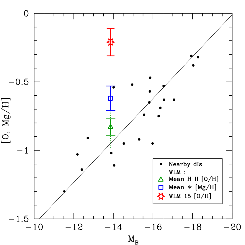
Figure 5.— Metallicity-luminosity relationship for dwarf irregular galaxies. The filled circles represent nebular oxygen abundances for the sample of nearby dwarfs, and the solid line is the best fit (Lee et al., 2003a, b). The open triangle indicates the mean nebular oxygen abundance derived in the present work; the vertical dotted line above and below the triangle marks the maximum ($-0.71$) and minimum ($-0.98$) derived values of the nebular oxygen abundance. The open square and the open star indicate the mean [Mg/H] for the two WLM supergiants and the stellar oxygen abundance for WLM 15, respectively (Venn et al., 2003, see also their Fig. 10).

Figure 6.— WLM in $U$, H$\alpha$, and H I. Dark objects on the image indicate bright sources. Left panel: H I contours superposed on a $U$-band image (Local Group Survey, Massey et al., 2002). Right panel: H I contours superposed on a continuum-subtracted H$\alpha$ image (Local Group Survey, Massey et al., 2002). Open circles surround H II regions where the reddening, $E(B-V)$, was found to be non-zero. In both panels, north is to the top and east is to the left, and the field of view shown is 6$\farcm$9 by 15$\farcm$3. The central rectangle in the right panel encompasses the 3$\farcm$2 by 3$\farcm$6 area shown in Fig. 1. The figures are adapted from Jackson et al. (2004).

Table 1 Basic data for WLM.

Property	Value	References
Type	IB(s)m	$\cdots$
Alternate Names	00DDO 221, UGCA 444 00	$\cdots$
Distance	$0.95\pm 0.04$ Mpc	1
Linear to angular scale at this distance	4.6 pc arsec-1	2
$B_{T}\,$	$11.03\pm 0.08$	3
$E(B-V)\,$	0.037	4
$F_{21}\,$	$299.8\pm 24.5$ Jy km s-1	5
$v_{\rm max}\,$	$38\pm 5$ km s-1	6
$[<{\rm Mg/H}>]$	$-0.62\pm 0.09$ ($\pm$ 0.26)	7
$[{\rm O/H}]$, WLM 15	$-0.21\pm 0.10$ ($\pm$ 0.05)	7
$[<{\rm O/H}>]$, H II	$-0.83\pm 0.06$	2

Table 2 Properties of EFOSC2 spectrograph employed at the ESO La Silla 3.6-m telescope.

Loral CCD (#40)
Total area	2048 $\times$ 2048 pix2
Field of view	5$\farcm$2 $\times$ 5$\farcm$2
Pixel size	15 $\mu$m
Image scale	0$\farcs$16 pixel-1
Gain	1.3 $e^{-}$ ADU-1
Read-noise (rms)	9 $e^{-}$
Long slit
Length	$\simeq 5$′
Width	1$\farcs$5
	Grating #11	Grating #7
Groove density	0300 lines mm-1 0	600 lines mm-1
Blaze $\lambda$ (1st order)	4000 Å	3800 Å
Dispersion	2.04 Å pixel-1	0.96 Å pixel-1
Effective $\lambda$ range	3380–7520 Å	3270–5240 Å

Table 3 Log of Observations.

H II	Date			00$t_{\rm total}$ 00			RMS
Region	(UT 2003)	Grating	$N_{\rm exp}$	(s)	$\langle X\rangle$	0[O III]$\lambda 4363$0	(mag)
(1)	(2)	(3)	(4)	(5)	(6)	(7)	(8)
HM 02	28 Aug	#11	1 $\times$ 1200	1200	1.24	no	0.034
HM 02	31 Aug	#7	3 $\times$ 1200	3600	1.21	no	0.025
HM 07	26 Aug	#11	3 $\times$ 1200	3600	1.06	yes	0.030
HM 08	26 Aug	#11	7 $\times$ 1200	8400	1.20	no	0.030
HM 09	26 Aug	#11	7 $\times$ 1200	8400	1.20	yes	0.030
HM 09	31 Aug	#7	3 $\times$ 1200	3600	1.21	no	0.025
HM 12	26 Aug	#11	3 $\times$ 1200	3600	1.06	no	0.030
HM 12	28 Aug	#11	3 $\times$ 1200	3600	1.08	no	0.034
HM 16 NW	27 Aug	#11	3 $\times$ 1200	3600	1.04	no	0.029
HM 16 SE	27 Aug	#11	3 $\times$ 1200	3600	1.04	no	0.029
HM 17	28 Aug	#11	3 $\times$ 1200	3600	1.03	no	0.034
HM 18	28 Aug	#11	3 $\times$ 1200	3600	1.03	no	0.034
HM 18a	28 Aug	#11	1 $\times$ 1200	1200	1.06	no	0.034
HM 18b	28 Aug	#11	1 $\times$ 1200	1200	1.06	no	0.034
HM 19	27 Aug	#11	3 $\times$ 1200	3600	1.04	no	0.029
HM 19	28 Aug	#11	3 $\times$ 1200	3600	1.08	no	0.034
HM 21	28 Aug	#11	3 $\times$ 1200	3600	1.08	no	0.034

Table 4a Line ratios and properties for H II regions HM 2 and HM 7.

		HM 2 (gr#7)		HM 2 (gr #11)		HM 7 (gr #11)
Wavelength (Å)	$f(\lambda)$	$F$	$I$	$F$	$I$	$F$	$I$
$[\rm{O\;II}]\;3727$	$+0.325$	$173\pm 13$	$198\pm 29$	$139.0\pm 8.9$	$136\pm 27$	$116.7\pm 1.9$	$116.1\pm 1.9$
${\rm H}11\;3772$	$+0.316$	$\cdots$	$\cdots$	$\cdots$	$\cdots$	$3.4\pm 1.4$	$4.2\pm 1.4$
${\rm H}10\;3799$	$+0.310$	$\cdots$	$\cdots$	$\cdots$	$\cdots$	$5.3\pm 1.6$	$6.2\pm 1.5$
${\rm H}9\;3835$	$+0.302$	$\cdots$	$\cdots$	$\cdots$	$\cdots$	$7.65\pm 0.91$	$8.77\pm 0.91$
$[{\rm Ne\;III}]\;3869$	$+0.294$	$55.3\pm 7.6$	$60\pm 13$	$48.8\pm 5.2$	$48\pm 11$	$39.25\pm 0.95$	$39.06\pm 0.95$
${\rm H}8+{\rm He\;I}\;3889$	$+0.289$	$\cdots$	$\cdots$	$\cdots$	$\cdots$	$22.33\pm 0.87$	$23.54\pm 0.87$
${\rm H}\epsilon+{\rm He\;I}\;3970$	$+0.269$	$36.1\pm 5.6$	$42\pm 10$	$21.2\pm 4.4$	$25.2\pm 9.5$	$27.84\pm 0.66$	$28.92\pm 0.66$
${\rm He\;I}\;4027$	$+0.253$	$\cdots$	$\cdots$	$\cdots$	$\cdots$	$1.96\pm 0.48$	$1.95\pm 0.48$
$[{\rm S\;II}]\;4068$	$+0.241$	$\cdots$	$\cdots$	$\cdots$	$\cdots$	$1.00\pm 0.59$	$1.00\pm 0.59$
${\rm H}\delta\;4101$	$+0.232$	$38.1\pm 6.1$	$43\pm 11$	$18.4\pm 2.5$	$21.6\pm 6.2$	$27.49\pm 0.77$	$28.43\pm 0.77$
${\rm H}\gamma\;4340$	$+0.158$	$42.9\pm 5.3$	$46.8\pm 9.6$	$48.6\pm 3.7$	$51\pm 11$	$47.2\pm 1.0$	$47.8\pm 1.0$
$[{\rm O\;III}]\;4363$	$+0.151$	$\cdots$	$\cdots$	$<12.3$	$<12.0$	$7.95\pm 0.80$	$7.91\pm 0.80$
${\rm He\;I}\;4388$	$+0.143$	$\cdots$	$\cdots$	$\cdots$	$\cdots$	$0.63\pm 0.81$	$0.63\pm 0.81$
${\rm He\;I}\;4471$	$+0.116$	$\cdots$	$\cdots$	$\cdots$	$\cdots$	$3.56\pm 0.25$	$3.54\pm 0.25$
$[{\rm Ar\;IV}]+{\rm He\;I}\;4713$	$+0.042$	$\cdots$	$\cdots$	$\cdots$	$\cdots$	$0.98\pm 0.17$	$0.98\pm 0.17$
$[{\rm Ar\;IV}]\;4740$	$+0.034$	$\cdots$	$\cdots$	$\cdots$	$\cdots$	$0.34\pm 0.14$	$0.34\pm 0.14$
${\rm H}\beta\;4861$	+0.000	$100.0\pm 5.7$	$100.0\pm 6.8$	$100\pm 11$	$100\pm 12$	$100.0\pm 3.7$	$100.0\pm 3.6$
$[{\rm O\;III}]\;4959$	$-0.026$	$187.9\pm 5.3$	$183\pm 20$	$213\pm 12$	$209\pm 39$	$133.9\pm 9.1$	$133.2\pm 9.1$
$[{\rm O\;III}]\;5007$	$-0.038$	$529.7\pm 6.4$	$516\pm 52$	$568\pm 15$	$556\pm 92$	$390\pm 12$	$388\pm 12$
${\rm He\;I}\;5876$	$-0.204$	$\cdots$	$\cdots$	$\cdots$	$\cdots$	$10.45\pm 0.38$	$10.40\pm 0.38$
$[{\rm O\;I}]\;6300$	$-0.264$	$\cdots$	$\cdots$	$\cdots$	$\cdots$	$2.89\pm 0.31$	$2.88\pm 0.31$
$[{\rm O\;I}]\;6363$	$-0.272$	$\cdots$	$\cdots$	$\cdots$	$\cdots$	$0.52\pm 0.24$	$0.51\pm 0.24$
${\rm H}\alpha\;6563$	$-0.299$	$\cdots$	$\cdots$	$280.0\pm 8.7$	$276\pm 47$	$270.5\pm 7.2$	$269.4\pm 7.2$
$[{\rm N\;II}]\;6583$	$-0.301$	$\cdots$	$\cdots$	$\cdots$	$\cdots$	$4.84\pm 0.59$	$4.81\pm 0.59$
${\rm He\;I}\;6678$	$-0.314$	$\cdots$	$\cdots$	$\cdots$	$\cdots$	$3.11\pm 0.30$	$3.09\pm 0.30$
$[{\rm S\;II}]\;6716$	$-0.319$	$\cdots$	$\cdots$	$\cdots$	$\cdots$	$7.57\pm 0.44$	$7.53\pm 0.44$
$[{\rm S\;II}]\;6731$	$-0.321$	$\cdots$	$\cdots$	$\cdots$	$\cdots$	$4.91\pm 0.38$	$4.89\pm 0.38$
${\rm He\;I}\;7065$	$-0.366$	$\cdots$	$\cdots$	$\cdots$	$\cdots$	$2.95\pm 0.21$	$2.94\pm 0.21$
$[{\rm Ar\;III}]\;7136$	$-0.375$	$\cdots$	$\cdots$	$\cdots$	$\cdots$	$5.87\pm 0.23$	$5.84\pm 0.23$
$[{\rm O\;II}]\;7320$	$-0.400$	$\cdots$	$\cdots$	$\cdots$	$\cdots$	$1.51\pm 0.22$	$1.50\pm 0.22$
$[{\rm O\;II}]\;7330$	$-0.401$	$\cdots$	$\cdots$	$\cdots$	$\cdots$	$1.84\pm 0.23$	$1.83\pm 0.23$
$F(\hbox{H$\beta$})$ (ergs s-1 cm-2)		$(4.54\pm 0.26)\times 10^{-16}$		$(2.47\pm 0.27)\times 10^{-15}$		$(4.63\pm 0.17)\times 10^{-15}$
EWe(H$\beta$) (Å)		$121\pm 20$		$98\pm 22$		$403\pm 114$
Derived $E(B-V)$ (mag)		$+0.087\pm 0.395$		$-0.038\pm 0.165$		$-0.061\pm 0.049$
$c(\hbox{H$\beta$})$		$\cdots$		$\cdots$		0
Adopted $A_{V}$ (mag)		$+0.28$		0		0
EWabs (Å)		2		2		2

Table 4b Line ratios and properties for H II region HM 9.

		HM 9 ap1 (gr#7)		HM 9 ap2 (gr #7)		HM 9 ap3 (gr #7)
Wavelength (Å)	$f(\lambda)$	$F$	$I$	$F$	$I$	$F$	$I$
$[\rm{O\;II}]\;3727$	$+0.325$	$264.5\pm 6.2$	$261\pm 20$	$301.6\pm 6.7$	$296\pm 22$	$407\pm 16$	$397\pm 47$
$[{\rm Ne\;III}]\;3869$	$+0.294$	$34.8\pm 3.7$	$34.3\pm 5.1$	$34.0\pm 4.4$	$33.4\pm 5.7$	$46\pm 11$	$45\pm 14$
${\rm H}\epsilon+{\rm He\;I}\;3970$	$+0.269$	$23.8\pm 2.5$	$26.6\pm 4.3$	$23.1\pm 2.5$	$26.4\pm 4.4$	$44.6\pm 8.1$	$48\pm 13$
${\rm H}\delta\;4101$	$+0.232$	$25.1\pm 2.2$	$27.8\pm 4.0$	$24.5\pm 2.2$	$27.5\pm 4.0$	$26.5\pm 6.5$	$30\pm 11$
${\rm H}\gamma\;4340$	$+0.158$	$45.7\pm 2.3$	$47.4\pm 4.8$	$47.8\pm 2.5$	$49.5\pm 5.0$	$54.7\pm 6.9$	$56\pm 12$
$[{\rm O\;III}]\;4363$	$+0.151$	$<7.3$	$<7.2$	$<8.3$	$<8.1$	$\cdots$	$\cdots$
${\rm H}\beta\;4861$	+0.000	$100.0\pm 2.2$	$100.0\pm 3.8$	$100.0\pm 2.2$	$100.0\pm 3.8$	$100.0\pm 5.8$	$100.0\pm 6.9$
$[{\rm O\;III}]\;4959$	$-0.026$	$102.6\pm 2.9$	$101.1\pm 8.0$	$93.9\pm 2.7$	$92.3\pm 7.4$	$70.7\pm 5.3$	$69\pm 10$
$[{\rm O\;III}]\;5007$	$-0.038$	$305.0\pm 3.5$	$300\pm 21$	$279.5\pm 3.3$	$275\pm 19$	$203.1\pm 6.4$	$198\pm 22$
$F(\hbox{H$\beta$})$ (ergs s-1 cm-2)		$(9.70\pm 0.21)\times 10^{-16}$		$(1.608\pm 0.036)\times 10^{-15}$		$(2.87\pm 0.17)\times 10^{-16}$
EWe(H$\beta$) (Å)		$132.5\pm 9.4$		$114.3\pm 7.2$		$80\pm 10$
Derived $E(B-V)$ (mag)		$-0.025\pm 0.195$		$-0.108\pm 0.197$		$-0.338\pm 0.409$
$c(\hbox{H$\beta$})$		$\cdots$		$\cdots$		$\cdots$
Adopted $A_{V}$ (mag)		0		0		0
EWabs (Å)		2		2		2
		HM 9 ap1 (gr#11)		HM 9 ap2 (gr #11)		HM 9 ap3 (gr #11)
Wavelength (Å)	$f(\lambda)$	$F$	$I$	$F$	$I$	$F$	$I$
$[\rm{O\;II}]\;3727$	$+0.325$	$208.7\pm 4.2$	$202\pm 11$	$215.9\pm 4.2$	$209\pm 12$	$213.4\pm 4.8$	$204\pm 12$
$[{\rm Ne\;III}]\;3869$	$+0.294$	$40.4\pm 1.7$	$39.1\pm 2.5$	$42.7\pm 1.2$	$41.3\pm 2.3$	$48.0\pm 2.3$	$45.9\pm 3.1$
${\rm H}8+{\rm He\;I}\;3889$	$+0.289$	$15.7\pm 1.4$	$23.0\pm 1.7$	$16.5\pm 1.0$	$24.3\pm 1.5$	$13.2\pm 1.8$	$24.5\pm 2.1$
${\rm H}\epsilon+{\rm He\;I}\;3970$	$+0.269$	$22.7\pm 1.5$	$29.1\pm 1.9$	$20.1\pm 1.1$	$27.2\pm 1.6$	$17.0\pm 2.0$	$27.4\pm 2.3$
${\rm H}\delta\;4101$	$+0.232$	$20.4\pm 1.5$	$26.3\pm 1.8$	$19.9\pm 1.1$	$26.1\pm 1.4$	$16.8\pm 1.6$	$25.8\pm 1.8$
${\rm H}\gamma\;4340$	$+0.158$	$45.6\pm 1.5$	$49.1\pm 1.9$	$45.3\pm 1.4$	$48.9\pm 1.8$	$43.5\pm 2.2$	$48.6\pm 2.5$
$[{\rm O\;III}]\;4363$	$+0.151$	$7.1\pm 1.1$	$6.9\pm 1.1$	$6.5\pm 1.1$	$6.3\pm 1.1$	$5.7\pm 1.7$	$5.4\pm 1.6$
${\rm He\;I}\;4471$	$+0.116$	$\cdots$	$\cdots$	$3.36\pm 0.67$	$3.25\pm 0.65$	$3.67\pm 0.90$	$3.50\pm 0.86$
${\rm H}\beta\;4861$	+0.000	$100.0\pm 3.9$	$100.0\pm 3.8$	$100.0\pm 3.8$	$100.0\pm 3.7$	$100.0\pm 4.2$	$100.0\pm 4.0$
$[{\rm O\;III}]\;4959$	$-0.026$	$143\pm 11$	$138\pm 11$	$140\pm 11$	$135\pm 11$	$135.1\pm 9.7$	$128.9\pm 9.3$
$[{\rm O\;III}]\;5007$	$-0.038$	$420\pm 14$	$406\pm 14$	$407\pm 14$	$394\pm 14$	$392\pm 12$	$374\pm 12$
${\rm He\;I}\;5876$	$-0.204$	$10.6\pm 1.1$	$10.3\pm 1.1$	$10.39\pm 0.78$	$10.05\pm 0.82$	$10.9\pm 1.5$	$10.4\pm 1.5$
${\rm H}\alpha\;6563$	$-0.299$	$279.9\pm 8.7$	$272\pm 16$	$287.3\pm 9.4$	$279\pm 16$	$295.0\pm 9.2$	$282\pm 16$
$[{\rm N\;II}]\;6583$	$-0.301$	$<4.6$	$<4.5$	$7.7\pm 2.3$	$7.5\pm 2.3$	$8.7\pm 1.8$	$8.3\pm 1.8$
$[{\rm S\;II}]\;6716,6731$	$-0.320$	$29.8\pm 1.8$	$28.8\pm 2.3$	$35.2\pm 1.7$	$34.0\pm 2.4$	$41.9\pm 2.6$	$39.9\pm 3.2$
$[{\rm Ar\;III}]\;7136$	$-0.375$	$8.7\pm 1.1$	$8.6\pm 1.6$	$8.00\pm 0.89$	$7.9\pm 1.3$	$8.9\pm 2.4$	$8.7\pm 2.8$
$F(\hbox{H$\beta$})$ (ergs s-1 cm-2)		$(2.67\pm 0.11)\times 10^{-16}$		$(6.52\pm 0.25)\times 10^{-16}$		$(1.942\pm 0.082)\times 10^{-16}$
EWe(H$\beta$) (Å)		$123\pm 11$		$111.0\pm 8.7$		$84.4\pm 6.1$
Derived $E(B-V)$ (mag)		$-0.036\pm 0.096$		$-0.012\pm 0.096$		$+0.009\pm 0.099$
$c(\hbox{H$\beta$})$		$-0.04\pm 0.07$		$-0.01\pm 0.07$		$+0.00\pm 0.07$
Adopted $A_{V}$ (mag)		0		0		0
EWabs (Å)		$4.1\pm 2.0$		$3.8\pm 1.4$		$4.1\pm 1.3$

Table 4c Line ratios and properties for H II regions HM 8, 12, 16, and 17.

		HM 8 (gr#11)		HM 12 (gr #11)		HM 12 (gr #11)
Wavelength (Å)	$f(\lambda)$	$F$	$I$	$F$	$I$	$F$	$I$
$[\rm{O\;II}]\;3727$	$+0.325$	$350\pm 15$	$339\pm 43$	$445\pm 12$	$432\pm 42$	$289.9\pm 9.9$	$281\pm 34$
$[{\rm Ne\;III}]\;3869$	$+0.294$	$\cdots$	$\cdots$	$\cdots$	$\cdots$	$37.1\pm 5.7$	$36.0\pm 8.3$
${\rm H}\delta\;4101$	$+0.232$	$\cdots$	$\cdots$	$\cdots$	$\cdots$	$22.2\pm 6.0$	$25\pm 10$
${\rm H}\gamma\;4340$	$+0.158$	$39.7\pm 4.9$	$40.7\pm 8.6$	$33.6\pm 3.3$	$36.9\pm 6.3$	$49.2\pm 5.6$	$51\pm 10$
${\rm H}\beta\;4861$	+0.000	$100.0\pm 6.5$	$100.0\pm 7.5$	$100.0\pm 4.5$	$100.0\pm 5.6$	$100.0\pm 6.1$	$100.0\pm 7.3$
$[{\rm O\;III}]\;4959$	$-0.026$	$46.9\pm 5.6$	$45.4\pm 9.0$	$40.1\pm 4.0$	$38.9\pm 6.2$	$75.6\pm 6.0$	$73\pm 12$
$[{\rm O\;III}]\;5007$	$-0.038$	$144.1\pm 7.0$	$140\pm 18$	$114.8\pm 4.8$	$111\pm 12$	$257.0\pm 8.0$	$249\pm 30$
${\rm He\;I}\;5876$	$-0.204$	$\cdots$	$\cdots$	$\cdots$	$\cdots$	$15.0\pm 3.3$	$14.6\pm 4.4$
${\rm H}\alpha\;6563$	$-0.299$	$266\pm 10$	$264\pm 33$	$284\pm 10$	$277\pm 29$	$288.5\pm 9.1$	$282\pm 34$
$[{\rm N\;II}]\;6583$	$-0.301$	$\cdots$	$\cdots$	$<7.7$	$<7.5$	$\cdots$	$\cdots$
$[{\rm S\;II}]\;6716,6731$	$-0.320$	$29.6\pm 5.1$	$28.7\pm 7.2$	$69.2\pm 7.2$	$67\pm 11$	$37.0\pm 4.6$	$36.0\pm 7.3$
$F(\hbox{H$\beta$})$ (ergs s-1 cm-2)		$(4.50\pm 0.29)\times 10^{-17}$		$(1.85\pm 0.08)\times 10^{-16}$		$(3.43\pm 0.21)\times 10^{-16}$
EWe(H$\beta$) (Å)		$62.2\pm 5.8$		$64.9\pm 4.3$		$66.5\pm 6.2$
Derived $E(B-V)$ (mag)		$-0.083\pm 0.124$		$-0.035\pm 0.106$		$-0.016\pm 0.121$
$c(\hbox{H$\beta$})$		$\cdots$		$\cdots$		$\cdots$
Adopted $A_{V}$ (mag)		0		0		0
EWabs (Å)		2		2		2
		HM 16 NW (gr#11)		HM 16 SE (gr #11)		HM 17 (gr #11)
Wavelength (Å)	$f(\lambda)$	$F$	$I$	$F$	$I$	$F$	$I$
$[\rm{O\;II}]\;3727$	$+0.325$	$309.0\pm 6.0$	$431\pm 33$	$470\pm 19$	$700\pm 94$	$448\pm 16$	$428\pm 55$
${\rm H}\epsilon+{\rm He\;I}\;3970$	$+0.269$	$13.2\pm 1.5$	$19.9\pm 3.6$	$\cdots$	$\cdots$	$\cdots$	$\cdots$
${\rm H}\delta\;4101$	$+0.232$	$17.1\pm 1.5$	$23.4\pm 3.4$	$\cdots$	$\cdots$	$\cdots$	$\cdots$
${\rm H}\gamma\;4340$	$+0.158$	$41.8\pm 1.6$	$48.9\pm 4.5$	$46.5\pm 7.6$	$60\pm 17$	$35.7\pm 6.1$	$39\pm 11$
$[{\rm O\;III}]\;4363$	$+0.151$	$<4.8$	$<5.3$	$\cdots$	$\cdots$	$\cdots$	$\cdots$
${\rm H}\beta\;4861$	+0.000	$100.0\pm 2.8$	$100.0\pm 4.1$	$100.0\pm 7.2$	$100.0\pm 8.3$	$100.0\pm 6.7$	$100.0\pm 7.9$
$[{\rm O\;III}]\;4959$	$-0.026$	$71.1\pm 4.6$	$68.8\pm 7.7$	$10.8\pm 5.5$	$9.9\pm 5.9$	$\cdots$	$\cdots$
$[{\rm O\;III}]\;5007$	$-0.038$	$214.2\pm 6.0$	$205\pm 17$	$13.2\pm 5.6$	$12.0\pm 6.2$	$56.6\pm 5.2$	$54.0\pm 9.6$
${\rm He\;I}\;5876$	$-0.204$	$10.6\pm 1.6$	$8.8\pm 1.7$	$\cdots$	$\cdots$	$\cdots$	$\cdots$
${\rm H}\alpha\;6563$	$-0.299$	$370.5\pm 8.3$	$286\pm 23$	$416\pm 13$	$286\pm 36$	$256.6\pm 9.8$	$248\pm 33$
$[{\rm N\;II}]\;6583$	$-0.301$	$14.2\pm 3.2$	$10.9\pm 3.0$	$\cdots$	$\cdots$	$\cdots$	$\cdots$
$[{\rm S\;II}]\;6716,6731$	$-0.320$	$26.5\pm 3.2$	$20.1\pm 3.3$	$64.8\pm 9.2$	$43.3\pm 9.9$	$42.6\pm 5.7$	$40.6\pm 8.9$
$F(\hbox{H$\beta$})$ (ergs s-1 cm-2)		$(6.86\pm 0.19)\times 10^{-16}$		$(1.38\pm 0.10)\times 10^{-16}$		$(2.39\pm 0.16)\times 10^{-16}$
EWe(H$\beta$) (Å)		$156\pm 13$		$34.6\pm 2.9$		$41.7\pm 3.3$
Derived $E(B-V)$ (mag)		$+0.251\pm 0.080$		$+0.332\pm 0.128$		$-0.145\pm 0.133$
$c(\hbox{H$\beta$})$		$\cdots$		$\cdots$		$\cdots$
Adopted $A_{V}$ (mag)		$+0.77$		$+1.0$		0
EWabs (Å)		2		2		2

Table 4d Line ratios and properties for H II regions HM 18, 18a, 18b, 19, and 21.

		HM 18 (gr#11)		HM 18a (gr #11)		HM 18b (gr #11)
Wavelength (Å)	$f(\lambda)$	$F$	$I$	$F$		$F$
$[\rm{O\;II}]\;3727$	$+0.325$	$790\pm 41$	$1000\pm 200$	$\cdots$		$\cdots$
${\rm H}\beta\;4861$	+0.000	$100\pm 10$	$100\pm 14$	$100\pm 19$		$100\pm 17$
${\rm H}\alpha\;6563$	$-0.299$	$618\pm 18$	$286\pm 54$	$554\pm 37$		$881\pm 50$
$[{\rm S\;II}]\;6716,6731$	$-0.320$	$92\pm 14$	$40\pm 12$	$\cdots$		$\cdots$
$F(\hbox{H$\beta$})$ (ergs s-1 cm-2)		$(9.50\pm 0.99)\times 10^{-17}$		$(1.47\pm.27)\times 10^{-16}$		$(7.6\pm 1.3)\times 10^{-17}$
EWe(H$\beta$) (Å)		$4.61\pm 0.48$		$8.8\pm 1.6$		$10.7\pm 1.9$
Derived $E(B-V)$ (mag)		$+0.445\pm 0.190$		$+0.481\pm 0.308$		$+0.982\pm 0.277$
$c(\hbox{H$\beta$})$		$\cdots$		$\cdots$		$\cdots$
Adopted $A_{V}$ (mag)		$+1.37$		$+1.48$		$+3.01$
EWabs (Å)		2		2		2
		HM 19 (gr#11)		HM 19 (gr #11)		HM 21 (gr #11)
Wavelength (Å)	$f(\lambda)$	$F$	$I$	$F$	$I$	$F$	$I$
$[\rm{O\;II}]\;3727$	$+0.325$	$350.2\pm 9.0$	$467\pm 48$	$131.6\pm 4.6$	$184\pm 16$	$387.0\pm 7.9$	$404\pm 38$
$[{\rm Ne\;III}]\;3869$	$+0.294$	$\cdots$	$\cdots$	$17.1\pm 3.0$	$22.4\pm 4.9$	$\cdots$	$\cdots$
${\rm H}\epsilon+{\rm He\;I}\;3970$	$+0.269$	$\cdots$	$\cdots$	$\cdots$	$\cdots$	$12.9\pm 2.4$	$18.5\pm 5.7$
${\rm H}\delta\;4101$	$+0.232$	$\cdots$	$\cdots$	$10.6\pm 1.6$	$24.0\pm 6.6$	$20.9\pm 2.2$	$26.1\pm 4.8$
${\rm H}\gamma\;4340$	$+0.158$	$39.2\pm 3.3$	$46.7\pm 7.5$	$30.0\pm 1.5$	$41.7\pm 4.7$	$43.6\pm 2.0$	$47.3\pm 5.5$
${\rm H}\beta\;4861$	+0.000	$100.0\pm 5.4$	$100.0\pm 6.3$	$100.0\pm 1.9$	$100.0\pm 4.0$	$100.0\pm 4.0$	$100.0\pm 5.4$
$[{\rm O\;III}]\;4959$	$-0.026$	$67.6\pm 5.0$	$65.0\pm 9.3$	$10.7\pm 1.4$	$9.9\pm 1.8$	$56.9\pm 3.8$	$55.2\pm 7.1$
$[{\rm O\;III}]\;5007$	$-0.038$	$177.7\pm 6.1$	$170\pm 18$	$36.4\pm 1.6$	$33.3\pm 3.2$	$175.7\pm 4.9$	$170\pm 17$
${\rm H}\alpha\;6563$	$-0.299$	$363\pm 14$	$286\pm 32$	$397.1\pm 4.0$	$286\pm 22$	$308.1\pm 7.6$	$286\pm 28$
$[{\rm N\;II}]\;6583$	$-0.301$	$\cdots$	$\cdots$	$6.7\pm 3.3$	$4.8\pm 2.6$	$<13$	$<12$
$[{\rm S\;II}]\;6716,6731$	$-0.320$	$\cdots$	$\cdots$	$8.4\pm 1.3$	$5.9\pm 1.1$	$35.3\pm 3.9$	$32.6\pm 5.6$
$F(\hbox{H$\beta$})$ (ergs s-1 cm-2)		$(3.78\pm 0.20)\times 10^{-16}$		$(9.24\pm 0.17)\times 10^{-16}$		$(6.70\pm 0.27)\times 10^{-16}$
EWe(H$\beta$) (Å)		$100\pm 11$		$35.54\pm 0.75$		$71.8\pm 4.6$
Derived $E(B-V)$ (mag)		$+0.223\pm 0.113$		$+0.285\pm 0.077$		$+0.050\pm 0.098$
$c(\hbox{H$\beta$})$		$\cdots$		$\cdots$		$\cdots$
Adopted $A_{V}$ (mag)		$+0.68$		$+0.87$		$+0.15$
EWabs (Å)		2		2		2

Table 5a Ionic and total abundances.

Property	HM 2	HM 2	HM 7	HM 8	HM 9 ap1	HM 9 ap2	HM 9 ap3
	(gr #7)	(gr #11)	(gr #11)	(gr #11)	(gr #7)	(gr #7)	(gr #7)
$T_{e}$(O+2) (K)	$\cdots$	0$<15800$ 0	$15350\pm 760$	$\cdots$	00$<16500$ 00	00$<18500$ 00	$\cdots$
$T_{e}$(O+) (K)	$\cdots$	$<14100$	$13750\pm 680$	$\cdots$	$<14600$	$<16000$	$\cdots$
O+/H $(\times 10^{5})$	$\cdots$	$>1.4$	$1.30\pm 0.21$	$\cdots$	$>2.4$	$>2.0$	$\cdots$
O+2/H $(\times 10^{5})$	$\cdots$	$>5.3$	$3.92\pm 0.45$	$\cdots$	$>2.5$	$>1.7$	$\cdots$
O/H $(\times 10^{5})$	$\cdots$	$>6.7$	$5.22\pm 0.50$	$\cdots$	$>4.9$	$>3.8$	$\cdots$
12$+$log(O/H)	$\cdots$	$>7.83$	00$7.72\pm 0.04\,(^{+0.05}_{-0.06})$ 00	$\cdots$	$>7.69$	$>7.58$	$\cdots$
12$+$log(O/H) M91	8.17	8.11	7.84	8.01	8.03	8.06	8.15
12$+$log(O/H) P00	7.92	7.85	7.67	8.18	7.92	7.99	8.23
Ar+2/H $(\times 10^{7})$	$\cdots$	$\cdots$	$2.47\pm 0.56$	$\cdots$	$\cdots$	$\cdots$	$\cdots$
Ar+3/H $(\times 10^{7})$	$\cdots$	$\cdots$	$0.25\pm 0.15$	$\cdots$	$\cdots$	$\cdots$	$\cdots$
ICF(Ar)	$\cdots$	$\cdots$	1.06	$\cdots$	$\cdots$	$\cdots$	$\cdots$
Ar/H $(\times 10^{7})$	$\cdots$	$\cdots$	$2.88\pm 0.61$	$\cdots$	$\cdots$	$\cdots$	$\cdots$
log(Ar/O)	$\cdots$	$\cdots$	$-2.25\pm 0.10$	$\cdots$	$\cdots$	$\cdots$	$\cdots$
N+/O+	$\cdots$	$\cdots$	$0.034\pm 0.004$	$\cdots$	$\cdots$	$\cdots$	$\cdots$
log(N/O)	$\cdots$	$\cdots$	$-1.46\pm 0.05$	$\cdots$	$\cdots$	$\cdots$	$\cdots$
Ne+2/O+2	$\cdots$	$\cdots$	$0.255\pm 0.027$	$\cdots$	$\cdots$	$\cdots$	$\cdots$
log(Ne/O)	$\cdots$	$\cdots$	$-0.594\pm 0.046$	$\cdots$	$\cdots$	$\cdots$	$\cdots$

Table 5b Ionic and total abundances (continued).

Property	HM 9 ap1	HM 9 ap2	HM 9 ap3	HM 12	HM 12	HM 16 NW
	(gr #11)	(gr #11)	(gr #11)	(gr #11)	(gr #11)	(gr #11)
$T_{e}$(O+2) (K)	$14100\pm 1000$	$13800\pm 1000$	$13300\pm 1800$	$\cdots$	$\cdots$	$<17300$
$T_{e}$(O+) (K)	$12890\pm 910$	$12650\pm 950$	$12300\pm 1600$	$\cdots$	$\cdots$	$<15100$
O+/H ($\times 10^{5}$)	$2.80\pm 0.68$	$3.10\pm 0.82$	$3.4\pm 1.6$	$\cdots$	$\cdots$	$>3.5$
O+2/H ($\times 10^{5}$)	$5.05\pm 0.87$	$5.24\pm 0.98$	$5.5\pm 1.9$	$\cdots$	$\cdots$	$>1.5$
O/H ($\times 10^{5}$)	$7.9\pm 1.1$	$8.3\pm 1.3$	$8.9\pm 2.4$	$\cdots$	$\cdots$	$>5.0$
12$+$log(O/H)	00$7.90\pm 0.06\,(^{+0.07}_{-0.09})$ 0	0$7.92\pm 0.06\,(^{+0.08}_{-0.09})$ 0	0$7.95\pm 0.11\,(^{+0.12}_{-0.18})$ 00	$\cdots$	$\cdots$	$>7.70$
12$+$log(O/H) M91	8.04	8.04	8.01	8.16	8.00	8.21
12$+$log(O/H) P00	7.85	7.86	7.84	8.48	7.96	8.29
Ar+2/H $(\times 10^{7})$	$4.2\pm 1.6$	$4.0\pm 1.4$	$4.7\pm 3.1$	$\cdots$	$\cdots$	$\cdots$
ICF(Ar)	1.50	1.48	1.48	$\cdots$	$\cdots$	$\cdots$
Ar/H $(\times 10^{7})$	$6.3\pm 2.4$	$5.9\pm 2.1$	$6.9\pm 4.5$	$\cdots$	$\cdots$	$\cdots$
log(Ar/O)	$-2.09\pm 0.19$	$-2.14\pm 0.18$	$-2.10\pm 0.36$	$\cdots$	$\cdots$	$\cdots$
N+/O+	$\cdots$	$0.027\pm 0.008$	$0.029\pm 0.007$	$\cdots$	$\cdots$	$\cdots$
log(N/O)	$\cdots$	$-1.57\pm 0.12$	$-1.53\pm 0.09$	$\cdots$	$\cdots$	$\cdots$
Ne+2/O+2	$0.251\pm 0.034$	$0.276\pm 0.034$	$0.327\pm 0.054$	$\cdots$	$\cdots$	$\cdots$
log(Ne/O)	$-0.600\pm 0.058$	$-0.558\pm 0.053$	$-0.485\pm 0.070$	$\cdots$	$\cdots$	$\cdots$
Property	HM 17	HM 19	HM 19	HM 21
	(gr #11)	(gr #11)	(gr #11)	(gr #11)
12$+$log(O/H) M91	8.17	8.24	7.64	8.14
12$+$log(O/H) P00	$\cdots$	8.40	8.12	8.28

Table 6 Comparison with previous spectroscopic data.

	STM89		HM95		Present work
Property	HM 2	HM 9	HM 7	HM 9	HM 7	HM 9
O/H ($\times 10^{5}$)	+$5\pm 3$	+$6\pm 3$	+$5.2\pm 0.8$	+$6.5\pm 1.1$	+$5.22\pm 0.50$	+$8.16\pm 0.79$
12$+$log(O/H)	+$7.70\pm 0.30$	+$7.78\pm 0.24$	+$7.72\pm 0.07$	+$7.81\pm 0.08$	+$7.72\pm 0.04$	+$7.91\pm 0.04$
log(N/O)	$\cdots$	$-1.3\pm 0.2$	$-1.60\pm 0.15$	$-1.00\pm 0.24$	$-1.46\pm 0.05$	$-1.55\pm 0.08$
log(Ne/O)	0$-0.8\pm 0.2$ 0	0$-0.6\pm 0.2$ 0	0$-0.87\pm 0.15$ 0	0$-0.94\pm 0.18$ 0	0$-0.594\pm 0.046$ 0	0$-0.562\pm 0.035$ 0
log(Ar/O)	$\cdots$	$-2.4\pm 0.2$	$-2.37\pm 0.14$	$-2.22\pm 0.18$	$-2.25\pm 0.10$	$-2.12\pm 0.12$

References

- Aller (1984) Aller, L. H. 1984, Physics of Thermal Gaseous Nebulae (Dordrecht: Reidel)
- Anders & Grevesse (1989) Anders, E., & Grevesse, N. 1989, Geochim. Cosmochim. Acta, 53, 197
- Asplund et al. (2004) Asplund, M., Grevesse, N., Sauval, A. J., Allende Prieto, C., & Kiselman, D. 2004, A&A, 417, 751
- Barnes & de Blok (2004) Barnes, D. G., & de Blok, W. J. G. 2004, MNRAS, 351, 333
- Battinelli & Demers (2004) Battinelli, P., & Demers, S. 2004, A&A, 416, 111
- Calura et al. (2003) Calura, F., Matteucci, F., & Vladilo, G. 2003, MNRAS, 340, 59
- Campbell et al. (1986) Campbell, A., Terlevich, R. J., & Melnick, J. 1986, MNRAS, 223, 811
- Cardelli et al. (1989) Cardelli, J. A., Clayton, G. C., & Mathis, J. S. 1989, ApJ, 345, 245
- DeRobertis et al. (1987) DeRobertis, M. M., Dufour, R. J., & Hunt, R. W. 1987, JRASC, 81, 195
- de Vaucouleurs et al. (1991) de Vaucouleurs, G., de Vaucouleurs, A., Corwin, H. G., Buta, R. J., Paturel, G., & Fouqué, P. 1991, Third Reference Catalog of Bright Galaxies (Berlin: Springer-Verlag)
- Dinerstein (1990) Dinerstein, H. L. 1990, in The Interstellar Medium in Galaxies, ed. H. A. Thronson & J. M. Shull (Dordrecht: Kluwer), 257
- Dolphin (2000) Dolphin, A. E. 2000, ApJ, 531, 804
- Ferraro et al. (1989) Ferraro, F. R., Fusi Pecci, F., Tosi, M., & Buonanno, R. 1989, MNRAS, 241, 433
- Garnett (1990) Garnett, D. R. 1990, ApJ, 363, 142
- Garnett (1992) Garnett, D. R. 1992, AJ, 103, 1330
- Garnett (2004) Garnett, D. R. 2004, in Cosmochemistry: The Melting Pot of the Elements, XIII Canary Islands Winter School of Astrophysics, eds. C. Esteban, R. J. García-López, A. Herrero, & F. Sánchez (Cambridge: Cambridge University Press), 171
- Gilmore & Wyse (1991) Gilmore, G., & Wyse, R. F. G. 1991, ApJ, 367, L55
- Grebel et al. (2003) Grebel, E. K., Gallagher, J. S., & Harbeck, D. 2003, AJ, 125, 1926
- Grevesse & Sauval (1996) Grevesse, N., & Sauval, A. J. 1998, Space Sci. Rev., 85, 161
- Hodge & Miller (1995) Hodge, P. W., & Miller, B. W. 1995, ApJ, 451, 176 (HM95)
- Hodge et al. (1999) Hodge, P. W., Dolphin, A. E., Smith, T. R., & Mateo, M. 1999, ApJ, 521, 577
- Hunter et al. (1993) Hunter, D. A., Hawley, W. N., & Gallagher, J. S. 1993, AJ, 106, 1797
- Izotov & Thuan (1999) Izotov, Y. I., & Thuan, T. X. 1999, ApJ, 511, 639
- Izotov et al. (1994) Izotov, Y. I., Thuan, T. X., & Lipovetsky, V. A. 1994, ApJ, 435, 647
- Jackson et al. (2004) Jackson, D. C., Skillman, E. D., Cannon, J. M., & Côté, S. 2004, AJ, 128, 1219
- Jacoby & Lesser (1981) Jacoby, G. H., & Lesser, M. P. 1981, AJ, 86, 185
- Kaufer et al. (2004) Kaufer, A., Venn, K. A., Tolstoy, E., Pinte, C., & Kudritzki, R. P. 2004, AJ, 127, 2723
- Kobulnicky & Skillman (1996) Kobulnicky, H. A., & Skillman, E. D. 1996, ApJ, 471, 211
- Kobulnicky & Skillman (1997) Kobulnicky, H. A., & Skillman, E. D. 1997, ApJ, 489, 636
- Kobulnicky et al. (1999) Kobulnicky, H. A., Kennicutt, R. C. Jr., & Pizagno, J. L. 1999, ApJ, 514, 544
- Krawchuk et al. (1997) Krawchuk, C. A. P., McCall, M. L., Komljenovic, M., Kingsburgh, R., Richer, M. G., & Stevenson, C. 1997, in IAU Symp. 180, Planetary Nebulae, ed. H. J. Habing and H. J. G. L. M. Lamers (Dordrecht: Kluwer), 116
- Lee (2001) Lee, H. 2001, Ph.D. thesis, York University
- Lee et al. (2003a) Lee, H., Grebel, E. K., & Hodge, P. W. 2003a, A&A, 401, 141
- Lee et al. (2003b) Lee, H., McCall, M. L., Kingsburgh, R., Ross, R., & Stevenson, C. C. 2003b, AJ, 125, 146
- Lee et al. (2003c) Lee, H., McCall, M. L., & Richer, M. G. 2003c, AJ, 125, 2975
- Lee & Skillman (2004) Lee, H., & Skillman, E. D. 2004, ApJ, 614, in press (astro-ph/0406571)
- Lennon & Burke (1994) Lennon, D. J. & Burke, V. M. 1994, A&AS, 103, 273
- Martin et al. (2004) Martin, N. F., Ibata, R. A., Bellazzini, M., Irwin, M. J., Lewis, G. F., & Dehnen, W. 2004, MNRAS, 348, 12
- Massey et al. (2002) Massey, P., Hodge, P. W., Holmes, S., Jacoby, G., King, N. L., Olsen, K., Smith, C., & Saha, A. 2002, BAAS, 34, 1272
- Matteucci (2003) Matteucci, F., 2003, Ap&SS, 284, 539
- McCall et al. (1985) McCall, M. L., Rybski, P. M., & Shields, G. A. 1985, ApJS, 57, 1
- McGaugh (1991) McGaugh, S. S. 1991, ApJ, 380, 140
- McGaugh (1994) McGaugh, S. S. 1994, ApJ, 426, 135
- McLaughlin & Bell (1993) McLaughlin, B. M., & Bell, K. L. 1993, ApJ, 408, 753
- Melotte (1926) Melotte, P. J., 1926, MNRAS, 86, 636
- Minniti & Zijlstra (1996) Minniti, D., & Zijlstra, A. A. 1996, ApJ, 467, L13
- Minniti & Zijlstra (1997) Minniti, D., & Zijlstra, A. A. 1997, AJ, 114, 147
- Moore et al. (2004) Moore, B. D., Hester, J. J., & Dufour, R. J. 2004, AJ, 127, 3484
- Olive & Skillman (2001) Olive, K. A., & Skillman, E. D. 2001, New Astronomy, 6, 119
- Osterbrock (1989) Osterbrock, D. E. 1989, Astrophysics of Gaseous Nebulae and Active Galactic Nuclei (Mill Valley: University Science Books)
- Pagel et al. (1979) Pagel, B. E. J., Edmunds, M. G., Blackwell, D. E., Chen, M. S., & Smith, G. 1979, MNRAS, 189, 95
- Pilyugin (2000) Pilyugin, L. S. 2000, A&A, 362, 325
- Pradhan (1976) Pradhan, A. K. 1976, MNRAS, 177, 31
- Prochaska et al. (2003) Prochaska, J. X., Gawiser, E., Wolfe, A. M., Castro, S., & Djorgovski, S. G. 2003, ApJ, 595, L9
- Rejkuba et al. (2000) Rejkuba, M., Minniti, D., Gregg, M. D., Zijlstra, A. A., Victoria Alonso, M., & Goudfrooij, P. 2000, AJ, 120, 801
- Richer & McCall (1995) Richer, M. G., & McCall, M. L. 1995, ApJ, 445, 642
- Rodríguez (2003) Rodríguez, M. 2003, ApJ, 590, 296
- Sandage & Carlson (1985) Sandage, A., & Carlson, G. 1985, AJ, 90, 1464
- Schlegel et al. (1998) Schlegel, D. J., Finkbeiner, D. P., & Davis, M. 1998, ApJ, 500, 525
- Shaw & Dufour (1995) Shaw, R. A., & Dufour, R. J. 1995, PASP, 107, 896
- Skillman (1989) Skillman, E. D. 1989, ApJ, 347, 883
- Skillman (1998) Skillman, E. D. 1998, in Stellar Astrophysics of the Local Group: VIII Canary Islands Winter School of Astrophysics, ed. A. Aparicio, A. Herrero, & F. Sánchez (Cambridge: Cambridge Univ. Press), 457
- Skillman et al. (1989a) Skillman, E. D., Kennicutt, R. C., Jr., & Hodge, P. 1989a, ApJ, 347, 875
- Skillman et al. (1989b) Skillman, E. D., Terlevich, R., & Melnick, J. 1989b, MNRAS, 240, 563 (STM89)
- Skillman et al. (2003a) Skillman, E. D., Côté, S., & Miller, B. W. 2003a, AJ, 125, 610
- Skillman et al. (2003b) Skillman, E. D., Tolstoy, E., Cole, A. A., Dolphin, A. E., Saha, A., Gallagher, J. S., Dohm-Palmer, R. C., & Mateo, M. 2003b, ApJ, 596, 253
- Storey & Hummer (1995) Storey, P. J., & Hummer, P. J. 1995, MNRAS, 272, 41
- Taylor & Klein (2001) Taylor, C. L., & Klein, U. 2001, A&A, 366, 811
- Tolstoy & Venn (2004) Tolstoy, E., & Venn, K. A. 2004, in Highlights of Astronomy, Vol. 13, as presented at the XXVth General Assembly of the IAU, Sydney, Australia, 14–25 August 2003, ed. O. Engvold, (San Francisco: Astron. Soc. Pacific), in press (astro-ph/0402295)
- Tolstoy et al. (2003) Tolstoy, E., Venn, K. A., Shetrone, M. D., Primas, F., Hill, V., Kaufer, A., & Szeifert, T. 2003, AJ, 125, 707
- Tomita et al. (1998) Tomita, A., Ohta, K., Nakanishi, K., Takeuchi, T. & Saito, M. 1998, AJ, 116, 131
- van Zee et al. (1998) van Zee, L., Salzer, J. J., Haynes, M. P., O’Donoghue, A. A., & Balonek, T. J. 1998, AJ, 116, 2805
- van Zee et al. (2004) van Zee, L., Skillman, E. D., & Haynes, M. P. 2004, AJ, 128, 121
- Venn et al. (2001) Venn, K. A., Lennon, D. J., Kaufer, A., McCarthy, J. K., Przybilla, N., Kudritzki, R. P., Lemke, M., Skillman, E. D., & Smartt, S. J. 2001, ApJ, 547, 765
- Venn et al. (2003) Venn, K. A., Tolstoy, E., Kaufer, A., Skillman, E. D., Clarkson, S. M., Smartt, S. J., Lennon, D. J., & Kudritzki, R. P. 2003, AJ, 126, 1326
- Venn et al. (2004a) Venn, K. A., Irwin, M., Shetrone, M. D., Tout, C. A., Hill, V., & Tolstoy, E. 2004a, AJ, 128, 1177
-
Venn et al. (2004b)
Venn, K. A., Tolstoy, E., Kaufer, A., & Kudritzki, R. P.
2004b, in Carnegie Observatories Astrophysics Series, Vol. 4:
Origin and Evolution of the Elements,
ed. A. McWilliam & M. Rauch (Pasadena: Carnegie Observatories,
http://www.ociw.edu/ociw/symposia/series/
symposium4/proceedings.html; also astro-ph/0305188) - Whiting et al. (1999) Whiting, A. B., Hau, G. K. T., & Irwin, M. 1999, AJ, 118, 2767
- Wiese et al. (1996) Wiese, W. L., Fuhr, J. R., & Deters, T. M. 1996, Atomic transition probabilities of carbon, nitrogen, and oxygen : a critical data compilation (American Chemical Society for the National Institute of Standards and Technology)
- Wolf (1910) Wolf, M. 1910, Astron. Nachr., 183, 187
- Yanny et al. (2003) Yanny, B. et al. 2003, ApJ, 588, 824 (erratum: 2004, ApJ, 605, 575)
- Zucker et al. (2004a) Zucker, D. B. et al. 2004a, ApJ, 612, L117
- Zucker et al. (2004b) Zucker, D. B. et al. 2004b, ApJ, 612, L121