On the Generation, Propagation, and Reflection of Alfvén Waves from the Solar Photosphere to the Distant Heliosphere

Abstract

We present a comprehensive model of the global properties of Alfvén waves in the solar atmosphere and the fast solar wind. Linear non-WKB wave transport equations are solved from the photosphere to a distance past the orbit of the Earth, and for wave periods ranging from 3 seconds to 3 days. We derive a radially varying power spectrum of kinetic and magnetic energy fluctuations for waves propagating in both directions along a superradially expanding magnetic flux tube. This work differs from previous models in three major ways. (1) In the chromosphere and low corona, the successive merging of flux tubes on granular and supergranular scales is described using a two-dimensional magnetostatic model of a network element. Below a critical flux-tube merging height the waves are modeled as thin-tube kink modes, and we assume that all of the kink-mode wave energy is transformed into volume-filling Alfvén waves above the merging height. (2) The frequency power spectrum of horizontal motions is specified only at the photosphere, based on prior analyses of G-band bright point kinematics. Everywhere else in the model the amplitudes of outward and inward propagating waves are computed with no free parameters. We find that the wave amplitudes in the corona agree well with off-limb nonthermal line-width constraints. (3) Nonlinear turbulent damping is applied to the results of the linear model using a phenomenological energy loss term. A single choice for the normalization of the turbulent outer-scale length produces both the right amount of damping at large distances (to agree with in situ measurements) and the right amount of heating in the extended corona (to agree with empirically constrained solar wind acceleration models). In the corona, the modeled heating rate differs by more than an order of magnitude from a rate based on isotropic Kolmogorov turbulence.

1 Introduction

Magnetic fields are known to play a significant role in determining the equilibrium state of the plasma in the solar atmosphere and solar wind (e.g., Parker 1975, 1991; Narain and Ulmschneider, 1990, 1996; Priest 1999). Much of the magnetic flux in the “quiet” photosphere seems to be concentrated into small (100–200 km) intergranular flux tubes. The physical processes that heat the chromosphere and corona have not yet been identified definitively, but there is little doubt that magnetohydrodynamic (MHD) effects are prevalent. Even many proposed nonmagnetic mechanisms depend on the underlying properties of the magnetically structured atmosphere. The outflowing solar wind is fed by open magnetic flux tubes, and many MHD processes have been proposed to deposit heat and momentum at locations ranging from the extended corona to interplanetary space.

The continually evolving convection below the photosphere gives rise to a wide spectrum of MHD fluctuations in the magnetic atmosphere and wind. The propagation of waves through the solar atmosphere has been studied for more than a half century (Alfvén 1947; Schwarzschild 1948; Biermann 1948). Although compressible (e.g., acoustic and magnetoacoustic) MHD waves are likely to be dynamically and energetically important in some regions of the atmosphere, it is the mainly incompressible Alfvén mode that has been believed for many years to be dominant in regions that are open to the heliosphere (e.g., Osterbrock 1961; Kuperus, Ionson, & Spicer 1981). Indeed, the MHD fluctuations measured by spacecraft in the solar wind have a strongly Alfvénic character (Belcher & Davis 1971; Hollweg 1975; Tu & Marsch 1995; Goldstein, Roberts, & Matthaeus 1995).

Even though much has been learned about the generation, propagation, reflection, and damping of Alfvén waves in the solar atmosphere, most earlier studies have focused on only a finite range of heights and treated the interactions with regions above or below as boundary conditions. This necessarily involved the approximation that the relevant phenomena are mainly local, i.e., that they do not depend on the conditions very far away from the region being modeled. There are circumstances, however, for which this approximation breaks down. For example, the properties of reflecting Alfvén waves with long periods (i.e., of order 1 day) in the solar wind depend formally on the conditions “at infinity,” since they behave asymptotically as standing waves (e.g., Heinemann & Olbert 1980).

In this paper we construct a comprehensive model of the radially evolving properties of Alfvénic fluctuations in a representative open magnetic region of the solar atmosphere and fast solar wind. The model takes account of nonlocal interactions by tracing the waves from their origin as transverse flux-tube oscillations in the photosphere all the way out to the interplanetary medium (truncated for convenience at 4 AU). This is done with the smallest possible number of free parameters. There are two overall aims of this paper:

1. We wish to understand better the global “energy budget” of Alfvén waves, including relative amplitudes of inward and outward propagating waves, along the open flux tubes that feed the solar wind.

2. In order to determine how MHD turbulence contributes to the heating of the extended solar corona, we need to pin down precisely how Alfvén waves provide the natural preconditions for a turbulent cascade.

The second aim above was motivated by a recent study of the small-scale dissipation of MHD turbulence in the extended corona (Cranmer & van Ballegooijen 2003). This kinetic dissipation depends strongly on how the turbulence is excited at its largest scales, and in this paper we attempt to put the “outer scale” wave dynamics on firmer footing so that the resulting “inner scale” can be better understood. The work described by this paper builds on prior studies by Hollweg (1973, 1978a, 1981, 1990), Heinemann & Olbert (1980), Spruit (1981, 1984), An et al.  (1990), Barkhudarov (1991), Velli (1993), Lou (1993, 1994), Lou & Rosner (1994), MacGregor & Charbonneau (1994), Kudoh & Shibata (1999), Matthaeus et al.  (1999), Hasan et al.  (2003), and many others.

One unique aspect of this paper is that the photospheric spectrum of transverse fluctuations—which constrains the Alfvén wave amplitudes at all larger radii—is specified directly from detailed observations of magnetic bright point (MBP) motions and is not (as in many other models) given as an arbitrary boundary amplitude. However, a complete physical description of the fluctuations in the photosphere (e.g., the relative inward/outward amplitudes and the kinetic/magnetic energy partition) is obtained only after the fully nonlocal wave reflection has been computed for all radii. Another way this work differs from many previous models is that the expansion and successive merging of flux tubes on granular and supergranular scales is described using a two-dimensional model of a magnetic network element in the inhomogeneous solar atmosphere.

Despite the attempted comprehensiveness of this model, we needed to make three specific approximations in order to render the calculations tractable. These approximations are summarized here, but they are also discussed further below and justified for certain regimes of applicability. First, we ignore all effects of compressible fluctuations (e.g., acoustic waves; fast and slow magnetosonic waves) despite their importance in understanding observed intensity oscillations and chromospheric heating. This is done in order to fairly assess the relative importance of the incompressible Alfvén mode before resorting to more involved models. Second, the Alfvén wave model is mainly linear, which limits its applicability in regions where the wave amplitudes become large in comparison to background field strengths and characteristic speeds. (Some effects of nonlinearity are examined, though, in § 6.) Third, we do not model explicitly the back-reaction of the waves on the mean properties of the solar atmosphere and solar wind. We do, however, compute quantities such as the wave pressure acceleration and turbulent heating rate for use in future models of this back-reaction.

The remainder of this paper is organized as follows. In § 2 we give an overview of the physical processes to be incorporated in the wave models together with a “cartoon” description of the steady-state magnetic field topology. In § 3 we describe the adopted steady-state (i.e., zero-order) plasma conditions in detail. The specification of the photospheric frequency spectrum of transverse fluctuations is given in § 4, and the wave equations to be solved are given in § 5. Solutions of these equations, including some with various prescriptions for damping, are presented in § 6. We conclude with a summary of major results (§ 7) and a discussion of remaining issues (§ 8). Appendix A contains supplementary equations describing analytic solutions of the kink-mode wave equations for isolated flux tubes in an isothermal atmosphere. Appendix B compares various published formalisms for the non-WKB transport equations for Alfvén waves in an accelerating wind. Appendix C summarizes the properties of the fully developed anisotropic MHD turbulence spectrum discussed by, e.g., Cranmer & van Ballegooijen (2003).

2 Overall Picture of Open Field Regions

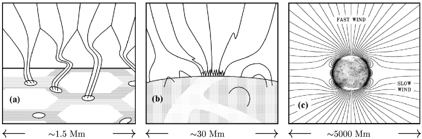
Figure 1: Summary sketch of the magnetic field structure discussed in this paper, with the fields of view successively widening from (a) to (b) to (c). (a) Intergranular lanes host G-band bright points that are shaken transversely to generate kink-mode waves. (b) Above the height where individual flux tubes merge, the coronal-hole network field is mainly open (with a funnel/canopy structure), and kink-mode waves are transformed into Alfvén waves. (c) Non-WKB waves in the solar wind propagate and reflect depending on their frequencies, and MHD turbulent cascade can occur where outward and inward waves interact nonlinearly. The inverted solar image was obtained by EIT (Extreme-ultraviolet Imaging Telescope) on SOHO (e.g., Moses et al.  1997). Field lines in (c) are plotted at 2.1° intervals at the solar surface, and thus each pair of lines encompasses $\sim$1–2 network funnels.

Figure 1 illustrates the basic magnetic field geometry that we believe is representative of flux tubes that feed the high-speed solar wind. A key feature of the adopted configuration is the successive merging of strong-field magnetic flux tubes between granules (Figure 1a) and supergranules (Figure 1b). On the largest scales, Figure 1c shows the more or less axisymmetric magnetic field that is characteristic of solar minimum (using the field model of Banaszkiewicz, Axford, & McKenzie 1998), but nearly all of the work presented in this paper can also be applied straightforwardly to open-field regions at other phases of the solar cycle.

We assert that most of the plasma that eventually becomes the time-steady solar wind originates in intergranular magnetic flux tubes known observationally as G-band bright points, network bright points, or in groups as “solar filigree.” This assertion is seemingly uncontroversial (knowing what we do about solar magnetic fields), though it is seldom stated. Adopting a ripening convention in nomenclature, we refer to these 100–200 km size photospheric features as magnetic bright points (MBPs). High-resolution observations reveal the presence of MBPs in the dark lanes between granules, and these features are associated with regions of strong (1–2 kG) magnetic field believed to be contained within nearly vertical flux tubes (e.g., Sheeley 1967; Dunn & Zirker 1973; Muller 1983, 1985; Piddington 1978; Rabin 1992; Solanki 1993; Berger & Title 2001). There is increasing evidence for magnetic structures on even smaller scales than 100–200 km, but we leave the study of these structures to future work (see, e.g., Stein & Nordlund 2002; Sánchez Almeida, Emonet, & Cattaneo 2003; Trujillo Bueno, Shchukina, & Asensio Ramos 2004).

As magnetic flux rises stochastically from the convection zone to the photosphere (e.g., Priest, Heyvaerts, & Title 2002), field lines are simultaneously jostled horizontally by fluid motions on granular (1–2 Mm) scales. Magnetic flux is concentrated into thin tubes by some combination of “flux expulsion” from the upflowing granule centers to the downflowing lanes (Parker 1963), the rapid evacuation of these downflowing superadiabatic regions (i.e., convective collapse; Parker 1978; Spruit 1979), and enhanced radiative cooling leading to thermal relaxation (Sánchez Almeida 2001). MBPs are observed frequently to merge with neighboring flux elements and to spontaneously fragment into several pieces (e.g., Berger et al.  1998). Once formed, MBPs continue to be shaken back and forth by the underlying convective motions (Kulsrud 1955; Osterbrock 1961; van Ballegooijen 1986; Huang, Musielak, & Ulmschneider 1995), which results in various kinds of wavelike fluctuations describable in the “thin-tube” MHD limit (Spruit 1981, 1982, 1984; see further references in § 5.1 below). Oscillatory motions can also be induced by impulsive reconnection events (e.g., Moore et al.  1991) or, conversely, the random wave trains may display observational time signatures that could be misinterpreted as small-scale flaring (Moriyasu et al.  2004).

There is a great variety of MHD wave activity expected and observed in the inhomogeneous solar atmosphere. In addition to isolated MBP fluctuations, there is ambient acoustic wave energy excited by convection, shock steepening in the chromosphere and transition region, and both driven and free oscillations in sunspots and coronal loops (see recent reviews by Axford et al.  1999; Roberts 2000; Bogdan 2000; Hirzberger 2003). A significant fraction of the Sun’s magnetic flux may also be distributed outside the MBPs, network, and active regions (e.g., Schrijver & Title 2003), and acoustic waves in “field-free” regions may in fact be magnetoacoustic. Damping of MHD waves and turbulence has been a key ingredient in many proposed models of chromospheric and coronal heating. Our main focus, though, is on the incompressible waves that eventually escape from the atmosphere into the solar wind.

Magnetic flux tubes rooted in MBPs undergo both transverse (kink-mode) and longitudinal (sausage-mode) oscillations that can propagate upward from the photosphere. Because the strong-field flux tubes are in horizontal pressure equilibrium with the surrounding weak-field material, they have a lower density and thus are susceptible to buoyancy effects and evanescence for long enough periods. Like acoustic waves, the compressible longitudinal modes steepen into shocks and damp over a few scale heights, while the incompressible kink modes can propagate into the corona relatively undamped. Nonlinear effects can lead to mode conversion between kink and longitudinal modes (e.g., Ulmschneider, Zähringer, & Musielak 1991).

Somewhere in the low chromosphere, the thin flux tubes are believed to expand laterally to the point where they merge with one another into a homogeneous network field distribution (Spruit 1984; Pneuman, Solanki, & Stenflo 1986; Gu et al.  1997). At this point, the thin-tube description breaks down and standard MHD wave theory becomes more applicable (i.e., kink modes become transverse Alfvén waves). The merged network flux bundles have horizontal scale lengths of 2 to 6 Mm and are probably maintained by large-scale convective flows that push the field to the edges of supergranular cells. At a larger height—still below the chromosphere-corona transition region—the network magnetic field expands laterally to 10–30 Mm scales and is thought to merge again into a large-scale “canopy” (e.g., Kopp & Kuperus 1968; Gabriel 1976; Giovanelli 1980; Anzer & Galloway 1983; Dowdy, Rabin, & Moore 1986). The spatial scale of the canopy is set by the typical distance between network flux bundles (i.e., the size of supergranulation cells) in the chromosphere. Observational evidence for preferential wind acceleration in the rapidly expanding network “funnels” is growing (Rottman, Orrall, & Klimchuk 1982; Hassler et al.  1999; Peter & Judge 1999; Aiouaz et al.  2004; see also Martínez-Galarce et al.  2003) but is still not definitive (e.g., Dupree, Penn, & Jones 1996).

As waves propagate upward into the corona, the radially varying Alfvén speed allows for gradual linear reflection (Ferraro & Plumpton 1958). The transition region can also act a sharp “reflection barrier” to Alfvén waves with wavelengths exceeding the local scale length of the Alfvén speed in that thin zone (see § 6). It is thus possible for a time-steady superposition of upward and downward propagating Alfvén waves to be maintained (e.g., Hollweg 1981, 1984). Strong reflection is not necessarily an impediment to there being a substantial upward wave flux; one merely needs more power in the upward modes than in the downward modes. Somewhere in the solar atmosphere the MHD fluctuations become turbulent, but it is unclear whether the turbulent cascade becomes energetically important in the photosphere (Petrovay 2001), in the chromosphere and transition region (Chae, Schühle, & Lemaire 1998), or in the corona (e.g., Dmitruk & Matthaeus 2003).

In the extended corona, the high-speed solar wind begins to accelerate supersonically above a heliocentric distance of 2 to 3 solar radii ($R_{\odot}$). In the radially inhomogeneous wind, the dissipationless propagation of MHD waves does work on the mean fluid and provides an added wave-pressure acceleration (e.g., Belcher 1971; Jacques 1977; Leer, Holzer, & Flå 1982). The presence of the wind also modifies how waves propagate, and above the Alfvén critical point—where the wind speed equals the local Alfvén speed at about 10 $R_{\odot}$—both the inward and outward modes are advected outward with the wind. Large coronal holes are the most probable source regions for the fast solar wind (for a review of observations and theoretical models, see Cranmer 2002). Some flux tubes in coronal holes have a higher density than the surrounding open-field plasma; these “polar plumes” seem to trace out the superradial expansion of the merged-canopy magnetic field in the corona (e.g., DeForest, Lamy, & Llebaria 2001).

In addition to Alfvén waves, there is some evidence for both fast-mode and slow-mode magnetosonic waves in the corona (Ofman, Nakariakov, & DeForest 1999; Nakariakov et al.  2004), but they have been observed only in relatively confined regions such as loops and plumes. Fast and slow modes are believed to be more attenuated by collisional damping processes than Alfvén waves before they reach the corona. However, once some fraction of the energy flux of Alfvén (and possibly fast-mode) waves escapes into the solar wind, the classical transport theory of collisional damping begins to break down and collisionless wave-particle interactions should dominate the damping (e.g., Hollweg & Isenberg 2002; Marsch, Axford, & McKenzie 2003; Cranmer 2000, 2001, 2002, 2004; and many references therein). Studies of wave-particle resonance damping have seen a recent resurgence of interest because of their potential importance in producing the preferential ion heating and acceleration seen both in the extended corona (Kohl et al.  1997, 1998, 1999) and in situ (Marsch 1999).

As Alfvén waves propagate into interplanetary space, their velocity and magnetic-field amplitudes grow to nonlinear magnitudes (i.e., $\delta B/B_{0}$ becomes of order unity). Higher order ponderomotive effects begin to dominate the wave propagation equations (Lau & Siregar 1996) and collisionless wave-wave resonances can create additional mode coupling and damping (Lee & Völk 1973; Lacombe & Mangeney 1980; Lou 1993). At some point it may even be inappropriate to use a “wavelike” paradigm to discuss the increasingly turbulent fluctuations (e.g., Goldstein et al.  1995). In the outer heliosphere, the description of magnetic flux tubes as relatively closed systems—implicit in the above discussion—breaks down as well, since processes such as stream-stream interactions, interstellar pickup ion injection, and cosmic ray transport increasingly dominate the physics.

In this paper we purposefully examine only a subset of the many processes listed above. This is done mainly to keep the modeling tractable, but it also helps clarify the extent to which the specific wave modes that we study can account for various observations.

3 Steady-State Plasma Conditions

Models of linear waves depend sensitively on the assumed background zero-order plasma properties (e.g., density, flow speed, magnetic field strength, flux tube geometry). In this section we describe the empirically constrained time-steady plasma along the central axis of a radially pointed (but superradially expanding) magnetic flux tube, from the photosphere to a distance of 4 AU. The empirical description consists of two parts: a two-dimensional magnetostatic model of thin MBP flux tubes that expand into the supergranular network canopy (§ 3.1) and a one-dimensional analytic continuation of the plasma parameters in the extended corona, assumed here to be along the axis of symmetry of a polar coronal hole at solar minimum (§ 3.2).

3.1 Network Magnetic Structure

We first develop a two-dimensional numerical model of a supergranular network element as a collection of thin flux tubes. The gas pressure in the atmosphere decreases with increasing height, causing a lateral expansion of the flux tubes. Neighboring MBP flux tubes within the network element merge into a monolithic structure at some height $z_{m}$. (Heights $z$ are measured from the optical-depth-unity photosphere; radii $r$ are measured from Sun center.) For a thin, isothermal flux tube in pressure equilibrium with its surroundings, the interior magnetic field strength varies with height as $e^{-z/2H}$, where $H$ is the pressure scale height (e.g., Spruit 1981, 1984). Thus we determine the so-called merging height by solving for

$$z_{m}\,\approx\,2H\ln(B_{\odot}/\bar{B})\,\,\,,$$ (1)

where $B_{\odot}$ is the field strength inside the flux tube at the base of the photosphere ($z=0$) and $\bar{B}$ is the average flux density in the network patch. Observations of the MBP flux-tube field strength range between 1000 and 2000 G, and the network-averaged field strength varies between about 20 and 300 G (e.g., Gabriel 1976; Giovanelli 1980). In order to determine a representative value for the merging height we use $H=120$ km, $B_{\odot}=1500$ G, and $\bar{B}=100$ G to obtain $z_{m}\approx 600$ km, a height in the low chromosphere (see also Pneuman et al.  1986). Above the merging height the network element consists of a single thick flux tube that further expands with height. The outer edge of this tube forms a magnetic canopy that overlies the neighboring supergranular cells. A second merging occurs when neighboring network elements come together at a “canopy height” $z_{c}$ above the supergranular cell centers; we set $z_{c}=1$ Mm (see also Hasan et al.  2003). Figure 2 shows the three-part structure of the network element:

1. The region below the merging height ($0<z<0.6$ Mm) is described as a collection of thin flux tubes embedded in a field-free medium. The field strength $B(z)$ is assumed to be the same for all flux tubes, and their cross sections and other plasma properties are consistent with the thin-tube approximation.

2. Between heights of 0.6 and 1 Mm, the merged network flux element expands laterally to the edges of the supergranular cell, which overlies a field-free cell-center chromosphere.

3. Between 1 and 12 Mm, the “fully merged” magnetic field fills the supergranular cell volume and expands primarily in the vertical direction.

In the remainder of this paper, the term “merging height” refers specifically to the merging of the thin flux tubes at $z_{m}=0.6$ Mm.

The total magnetic flux $\Phi$ of the network element is constrained empirically to be $3.7\times 10^{19}$ Mx. The MBP field strengths at the photosphere and at the merging height are 1430 G and 120.4 G, respectively. The upper, monolithic part of the magnetic structure ($z>z_{m}$) is assumed to be cylindrically symmetric and is described by a modified version of the magnetostatic flux tube model of Hasan et al.  (2003). In the present case, the flux tube is contained within a cylinder of transverse radius $s_{0}=10$ Mm, which simulates the effect of neighboring network elements. The internal and external gas pressures are taken from semiempirical VAL/FAL models by Vernazza, Avrett, & Loeser (1981) and Fontenla, Avrett, & Loeser (1990, 1991, 1993, 2002). The magnetic field components $B_{s}(s,z)$ and $B_{z}(s,z)$ in cylindrical geometry (using $s$ as the perpendicular distance from the central flux tube axis) are computed by varying the shapes of the field lines until a minimum-energy state is obtained (for details see Hasan et al.  2003). The horizontal distribution of $B_{z}(s,z_{m})$ at the merging height is adjusted iteratively such that the magnitude of the field $B(s,z_{m})$ is independent of $s$. This is needed for consistency with the constant field strength of the thin flux tubes just below the merging height.

Figure 2 shows the final iterated magnetic structure. The cross sections of the flux tubes below the merging height ($z<0.6$ Mm) were computed by matching $B_{s}$ and $B_{z}$ at the merging height and assuming that $B_{s}$ is independent of height within each flux tube (different tubes have different $B_{s}$). The transverse radius of the “network patch” in the photosphere is about 3 Mm. We can estimate the number $N$ of MBPs inside the approximately circular patch, but we note that the wave analysis below does not depend on the value of $N$. From the conservation of magnetic flux, we know that the filling factor of MBP flux tubes at the photosphere is given by $B(z_{m})/B_{\odot}\approx 0.08$. Observationally, the transverse radii of MBPs at the photosphere are 50 to 100 km. The number of flux tubes required to fill an area that is 8% of the total patch area ($A=\pi s_{\odot}^{2}$, with $s_{\odot}=3$ Mm) ranges between $N\approx 75$ (for the upper limit on MBP radius) and $N\approx 300$ (for the lower limit). We can also define a mean distance between nearest neighbors $d_{nn}$ by dividing up up the network patch into $N$ equal-area circles and defining $d_{nn}$ as twice their radii. Thus, $d_{nn}=2s_{\odot}N^{-1/2}$, which gives values of 350 and 700 km for the above limiting cases.

Before continuing, it is worthwhile to ask the question: “Why is it not possible to extend the ‘monolithic’ flux-tube model all the way down to the photosphere?” Observationally, the photosphere is far from monolithic in its distribution of magnetic fields. Granulation causes both the formation of thin MBP flux tubes and their spreading out (via random walk). The larger-scale supergranulation pushes the magnetic elements back together into network lanes and vertices. This competition between MBP spreading and convergence leads to a dynamical equilibrium described by the different assumptions applied above and below the merging height. A more complete model must contain physics that naturally captures this equilibrium state, but hopefully without the abrupt transition assumed here at $z_{m}$.

3.2 Superradial Expansion in the Solar Wind

Here we describe the plasma parameters along the central axis of the modeled network element at heights ranging from 12 Mm (the top of the magnetostatic model) to interplanetary space. We adopt a slightly modified version of the polar magnetic field configuration of Banaszkiewicz et al.  (1998):

$$\frac{B_{0}}{1.789\mbox{\, G}}\,=\,\frac{2}{x^{3}}+\frac{4.281}{x^{5}}+\frac{1}{a_{c}(x+a_{c})^{2}}+\frac{0.67}{\exp[384(x-x_{0})]}$$ (2)

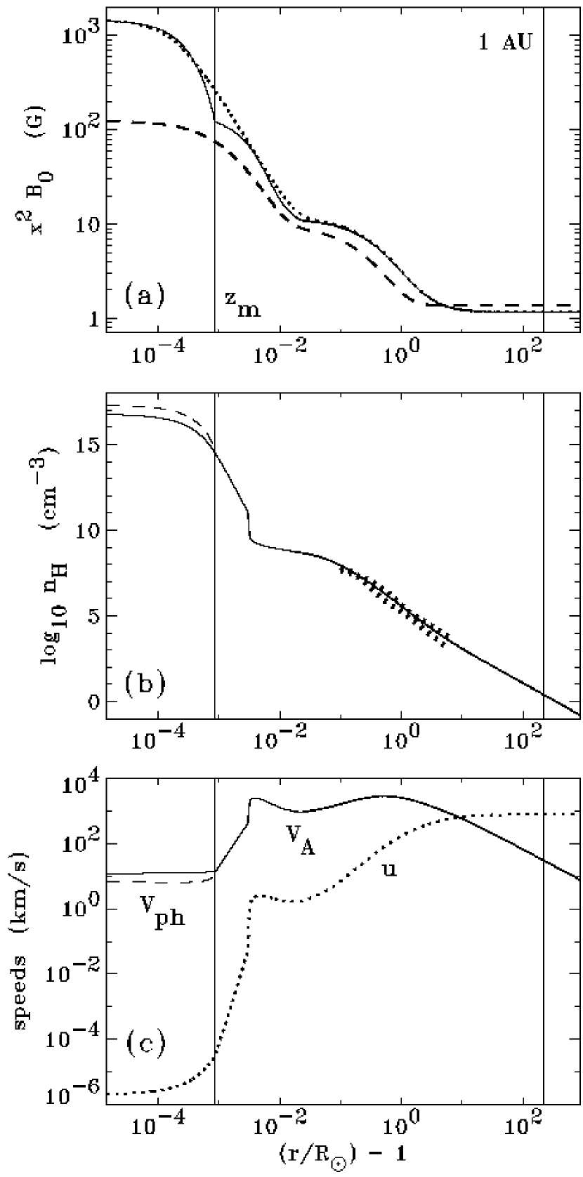
Figure 3: Steady-state plasma conditions along the central axis of the network flux tube. (a) Magnetic field strength, multiplied by $x^{2}$, for the adopted model (solid line), the model of Hackenberg et al.  (2000) (dotted line), and the model of Li (2003) (dashed line). (b) Adopted model of the hydrogen number density (solid line), empirical limits taken from the minima and maxima of observations by Guhathakurta & Holzer (1994), Fisher & Guhathakurta (1995), and Doyle et al.  (1999) (dotted lines), and the quantity $\rho_{\rm tot}/1.2/m_{\rm H}$ (dashed line). (c) Alfvén speed $V_{A}$ (solid line), outflow speed $u$ (dotted line), and flux tube phase speed $V_{\rm ph}$ (dashed line).

where $B_{0}$ is now defined as the radial component of the field along the axis of symmetry, $x=r/R_{\odot}$, and the above description applies only for $x\geq x_{0}$, with $x_{0}\equiv 1.0172$ (i.e., the top height [12 Mm] of the magnetostatic grid). The model above uses the same current-sheet constant ($a_{c}=1.538$) used by Banaszkiewicz et al.  (1998), but with a 5% modification to their preferred quadrupole constant. We also add an exponential correction term (which drops rapidly to nearly zero for $x\gtrsim 1.03$) to ensure that the value and slope of $B_{0}$ match those of the magnetostatic model at $x_{0}$. Figure 3a plots the product $x^{2}B_{0}$ versus height both below and above $x_{0}$. This quantity is proportional to the inverse of the traditional superradial divergence factor $f$, and it shows the outer monopolar expansion region ($B_{0}\propto r^{-2}$) as a constant. For comparison we also plot the analytic functions used in the funnel models of Hackenberg, Marsch, & Mann (2000) and Li (2003).

For the radial dependence of the electron density, we use a function motivated by fits to white-light polarization brightness measurements in the extended corona:

$$\frac{n_{e}}{1.3\times 10^{5}\mbox{\, cm}^{-3}}\,=\,\frac{1}{x^{2}}+\frac{25}{x^{4}}+\frac{300}{x^{8}}+\frac{1500}{x^{16}}+\frac{5796}{x^{33.9}}$$ (3)

which applies only for $x\geq x_{0}$. The overall scale set by the inverse square term was adjusted to match in situ density measurements at 1 AU (i.e., $x=215$). The middle three terms above were adjusted to produce agreement with measurements by, e.g., Guhathakurta & Holzer (1994), Fisher & Guhathakurta (1995), Doyle, Teriaca, & Banerjee (1999), Esser & Sasselov (1999), and Figure 10 of Lie-Svendsen, Hansteen, & Leer (2003). The last term was set to match the value and slope of the magnetostatic model density at $x_{0}$. Figure 3b plots the hydrogen number density $n_{\rm H}$, computed assuming a helium-to-hydrogen number density ratio of 0.05 (i.e., $n_{e}=1.1\,n_{\rm H}$, with the total mass density $\rho$ given by $1.2\,n_{\rm H}m_{\rm H}$).

Figure 3c shows several velocity quantities along the central axis of the flux tube. The hydrogen outflow speed $u$ was computed by mass flux conservation (i.e., $\rho u/B_{0}=$ constant), with the mass loss rate set by Ulysses measurements in interplanetary space (Goldstein et al.  1996). At 1 AU, the product $un_{\rm H}=2\times 10^{8}$ cm^-2 s^-1, and thus we compute $u=781.2$ km s^-1 at 1 AU. At an infinite distance, $u$ approaches a constant value of 781.9 km s^-1. The Alfvén speed, defined as

$$V_{A}\,\equiv\,B_{0}/\sqrt{4\pi\rho}\,\,\,,$$ (4)

is nearly constant below the merging height (and would be precisely constant for an isothermal atmosphere) and rises to two successive maxima: 2530 km s^-1 at $r=1.004\,R_{\odot}$, and 2890 km s^-1 at $r=1.53\,R_{\odot}$. The Alfvén speed drops to 31.3 km s^-1 at 1 AU and decreases nearly exactly as $1/r$ after that. The Alfvén critical point, where $u=V_{A}$, is at $r_{A}=9.70\,R_{\odot}$.

4 Photospheric Fluctuation Spectrum

The lower boundary condition for our model of Alfvénic fluctuations is the power spectrum of transverse MBP motions in the photosphere. The dynamical behavior of G-band bright points has been studied observationally by a number of groups (see, e.g., Muller et al.  1994; Berger & Title 1996; van Ballegooijen et al.  1998; Berger et al.  1998; Krishnakumar & Venkatakrishnan 1999; Nisenson et al.  2003). In this section we present an empirical description of MBP dynamics as a linear superposition of two types of motion: (1) the “random walk” undertaken by isolated flux tubes, and (2) a series of rapid “jumps” that occur when individual flux tubes merge, fragment, or reconnect with surrounding magnetic field.

The general procedure for specifying the power spectrum of horizontal MBP kinetic energy (as a function of frequency) is illustrated in Figure 4. The primary measured quantity is a time series of discrete position measurements for the MBPs which can be differentiated to obtain horizontal velocity components $v_{x}(t)$ and $v_{y}(t)$, with the $z$ direction being normal to the solar surface. (Observations support the rational assumption that there is no preferred global direction on granular scales, so below we discuss just the $v_{x}$ component and assume that $v_{y}$ is statistically equivalent.) The timescale dependence of MBP fluctuations is encapsulated in the velocity autocorrelation function, which we define for a time sequence of $N$ measured velocities $v_{x,n}$ as

$$C_{xx,m}\,=\,\frac{1}{N-m}\sum_{n=1}^{N-m}v_{x,n}\,v_{x,n+m}$$ (5)

for the time index $n$ between 1 and $N$ and an arbitrary delay time represented by index $m$. This expression is the discrete version of the more general definition

$$C_{xx}(\tau)\,=\,\lim_{\Delta t\rightarrow\infty}\frac{1}{\Delta t}\int_{-\Delta t/2}^{+\Delta t/2}dt\,v_{x}(t)\,v_{x}(t+\tau)$$ (6)

for delay time $\tau$. The unidirectional power spectrum $P_{x}$ (i.e., $|v_{x}|^{2}$ per unit interval of frequency $\omega$) is the Fourier transform of the autocorrelation function, with

$$P_{x}(\omega)\,\equiv\,\frac{1}{2\pi}\int_{-\infty}^{+\infty}d\tau\,C_{xx}(\tau)\,e^{i\omega\tau}$$ (7)

(e.g., the Wiener-Khinchin theorem; see also van Ballegooijen et al.  1998). Note that $P_{x}$ is defined for both positive and negative $\omega$. For the present applications, all functions are symmetric about zero frequency, and we will thus consider only positive frequencies (simultaneously doubling the normalization of $P_{x}$ to conserve total energy). In general, we specify the kinetic energy power spectrum $P_{K}$, which is defined in such a way as to integrate to the total kinetic energy density $U_{K}$ in transverse motions:

$$U_{K}\,\equiv\,\frac{\rho\langle\delta V\rangle^{2}}{2}\,=\,\int_{0}^{\infty}d\omega\,P_{K}(\omega)\,\,\,,$$ (8)

with

$$P_{K}(\omega)\,\equiv\,\frac{\rho}{2}\left[2P_{x}(\omega)+2P_{y}(\omega)\right]\,=\,2\rho P_{x}(\omega)\,\,\,.$$ (9)

The factors of two inside the square brackets take account of the negative frequencies, and the last expression assumes $P_{x}=P_{y}$.

In the analysis below we derive power spectrum components for the two assumed phases of the MBP motion: the random walk (subscript $w$) of isolated flux tubes, and the occasional discrete jumps (subscript $j$) caused by merging, fragmenting, or reconnecting. Specifying the power separately for these two phases is not the ideal solution, but it is all that can be done at present. Ideally, the proper observational procedure would be to determine the complete time series $v_{x}(t)$ for the walk and jump phases taken together, then compute the autocorrelation function and total power spectrum consistently. Unfortunately, because MBPs fragment or merge during the jump phases, it is extremely difficult to “follow” a single feature during these times to determine the complete time series.

The random-walk component of MBPs, during the times they exist as separate entities, was studied by van Ballegooijen et al.  (1998) and Nisenson et al.  (2003). These observations yielded the result that the discretely derived autocorrelation functions can be fit well by Lorentzian functions (see Figure 4e), with

$$C_{xx,w}(\tau)\,=\,\frac{\sigma_{w}^{2}}{1+(\tau/\tau_{w})^{2}}$$ (10)

and the more precise observations of Nisenson et al.  (2003) gave values of $\sigma_{w}^{2}\approx 0.8$ km² s^-2 and $\tau_{w}\approx 60$ s. We adopt these values in the models below. Thus, the walk-component of the kinetic energy spectrum is given by

$$P_{K,w}(\omega)\,=\,\rho\sigma_{w}^{2}\tau_{w}e^{-\tau_{w}\omega}\,\,\,.$$ (11)

This is plotted in Figure 4g, but note that all power spectra are plotted as the product $\omega P(\omega)$ because this denotes the power per decade of frequency (i.e., the energy density per unit $\log\omega$). Maxima in this quantity highlight the frequencies that contribute most to the total wave energy.

The impulsive “jump” phase of MBP motions is described by Choudhuri, Dikpati, & Banerjee (1993), Berger et al.  (1998), Hasan, Kalkofen, & van Ballegooijen (2000), and others. The potential for rapid transitions in the locations of thin flux tubes is also indicated in empirical models of the quasi-equilibrium evolution of granular magnetic fields (van Ballegooijen & Hasan 2003), in which slow motions of separatrix surfaces in the photosphere are amplified at larger heights due to flux-tube expansion. We model an impulsive MBP event as narrow Gaussian enhancement in $v_{x}(t)$ centered on an arbitrary $t=0$. A series of these events is assumed to occur with a mean time interval $\Delta t$ between events. The Gaussian jump, with velocity amplitude $\sigma_{j}$ and $1/e$ half-life $\tau_{j}$, is described by

$$v_{x}(t)\,=\,\sigma_{j}e^{-(t/\tau_{j})^{2}}$$ (12)

between times $-\Delta t/2$ and $+\Delta t/2$, and the limit $\Delta t\rightarrow\infty$ in eq. (6) is not taken. The autocorrelation function is thus

$$C_{xx,j}(\tau)\,=\,\sqrt{\frac{\pi}{2}}\,\frac{\sigma_{j}^{2}\tau_{j}}{\Delta t}\exp\left(-\frac{\tau^{2}}{2\tau_{j}^{2}}\right)$$ (13)

(see Figure 4f) and the resulting kinetic energy spectrum is given by

$$P_{K,j}(\omega)\,=\,\frac{\rho\sigma_{j}^{2}\tau_{j}^{2}}{\Delta t}\exp\left(-\frac{\omega^{2}\tau_{j}^{2}}{2}\right)$$ (14)

(see Figure 4h). In the models below we adopt $\Delta t=360$ s and $\tau_{j}=20$ s, which are consistent with the observations of Berger et al.  (1998). The velocity amplitude of the jump $\sigma_{j}$ is known with much less certainty because it represents the “tail” of the observed distribution of speeds. Berger & Title (1996) found speeds up to 5 km s^-1, so this seems to be a rough upper limit to $\sigma_{j}$. This is our only true free parameter.

Because the walk and jump phases of MBP motion seem to be statistically uncorrelated, we compute the full kinetic energy spectrum $P_{K}$ as the simple sum of $P_{K,w}$ and $P_{K,j}$ (see Figure 4i). It is then possible to integrate this spectrum over frequency (see eq. [8]) to obtain the transverse velocity variance of MBP motions in the photosphere:

$$\langle\delta V\rangle^{2}_{\odot} = 2\sigma_{w}^{2}+\sqrt{2\pi}\,\sigma_{j}^{2}\tau_{j}/\Delta t$$ (15)

$$= \left[1.6\,+\,0.139\left(\frac{\sigma_{j}}{1\,\mbox{km}\,\mbox{s}^{-1}}\right)^{2}\right]\,\mbox{km}^{2}\,\mbox{s}^{-2}$$ (16)

where the latter expression uses the values adopted above for $\sigma_{w}$, $\tau_{j}$, and $\Delta t$. Note that even for a large impulsive velocity of $\sigma_{j}\approx 6$ km s^-1, the root-mean-squared velocity is significantly smaller than this value ($\langle\delta V\rangle_{\odot}\approx 2.5$ km s^-1) because the jumps occur infrequently.

Finally, we also compute the total energy spectrum $P_{\rm tot}$ (i.e., including contributions from both kinetic and magnetic energy) at the photosphere using the analytic relations for isothermal thin flux tubes given in Appendix A (specifically, eq. [A8]). For very high frequencies the kinetic and magnetic energy components are in equipartition, and $P_{\rm tot}$ is just twice $P_{K}$. For very low frequencies the kink-mode waves are evanescent and the physically realistic solution contains much more kinetic energy than magnetic energy (thus, $P_{\rm tot}\approx P_{K}$). The resulting total energy spectrum, plotted as a solid line in Figure 4i, is essentially our lower boundary condition on the amplitudes of Alfvén waves of various frequencies. We describe how this information is folded into the global solutions in § 5.3.

5 Non-WKB Wave Analysis

We model the transverse wave properties in the open magnetic regions described in § 3 as purely linear perturbations to the assumed zero-order background plasma state. The basic MHD equations that need to be solved are the mass and momentum conservation equations and the magnetic induction equation, given by

$$\frac{\partial\rho}{\partial t}+\nabla\cdot(\rho{\bf v})\,=\,0$$ (17)

$$\frac{\partial{\bf v}}{\partial t}+({\bf v}\cdot\nabla){\bf v}\,=\,-\frac{1}{\rho}\nabla p+{\bf g}+\frac{1}{4\pi\rho}\left[(\nabla\times{\bf B})\times{\bf B}\right]$$ (18)

$$\frac{\partial{\bf B}}{\partial t}\,=\,\nabla\times\left({\bf v}\times{\bf B}\right)$$ (19)

where the velocity ${\bf v}$ and magnetic field ${\bf B}$ are not yet separated into zero-order and first-order parts, $p$ is the gas pressure, and ${\bf g}$ is the gravitational acceleration.

We apply these equations in two regions with very different physics:

1. Below the merging height (§ 5.1) we model the waves as incompressible Lagrangian perturbations of the central axis of a thin, strong-field flux tube that expands superradially and is surrounded by a field-free region. In this region we assume the outflow speed of the solar wind is negligibly small. In addition to the properties within the thin tube, we also specify the density external to the tube $\rho_{e}$ in the field-free region.

2. Above the merging height (§ 5.2) we model the waves as incompressible Eulerian perturbations filling the volume of the expanding flux tube, which is assumed to be surrounded by similar tubes. All background properties, including a nonzero solar wind speed, vary only in the radial direction.

For both regions we transform the MHD equations above into wave equations with an assumed $e^{i\omega t}$ time dependence. The equations are then solved “monochromatically” for a grid of frequencies, also assuming that in each solution the frequency remains constant as a function of height. We do not make the WKB (i.e., eikonal) approximation that wavelengths are small compared to background scale lengths; indeed we do not even need to define the concept of wavelength because the complete spatial oscillation pattern is computed numerically as a function of height. The solutions for individual frequencies are subsequently assembled into a full radially varying power spectrum, normalized by the empirically derived power spectrum at the photosphere (§ 4).

The following subsections present the specific equations that we solve in the two regions outlined above.

5.1 Thin Flux Tubes

Below the merging height, the MBP flux tubes are shaken transversely and kink-mode waves are excited (see also Wilson 1979; Spruit 1981; Ulmschneider et al.  1991). For incompressible perturbations about the equilibrium state, the density $\rho$ is a zero-order quantity, the velocity ${\bf v}$ is horizontal and a first-order quantity, and the magnetic field ${\bf B}$ has a zero-order vertical component and a first-order horizontal component. Following the motion of the thin tubes, we write the Lagrangian forms of the momentum and induction equations as follows:

$$\rho\frac{d{\bf v}}{dt}\,=\,\rho{\bf g}-\nabla\left(p+\frac{B^{2}}{8\pi}\right)+\frac{({\bf B}\cdot\nabla){\bf B}}{4\pi}$$ (20)

$$\frac{d{\bf B}}{dt}\,=\,\left({\bf B}\cdot\nabla\right){\bf v}$$ (21)

where the advective derivative

$$\frac{d}{dt}\,=\,\frac{\partial}{\partial t}+{\bf v}\cdot\nabla$$ (22)

follows the motion of the tube’s central axis. Above we have assumed that $\nabla\cdot{\bf v}=0$ as a statement of mass conservation for incompressible flows.

We write the scalar horizontal perturbations in velocity and magnetic field as $v_{\perp}$ and $B_{\perp}$, and we implicitly assume linear polarization of the waves in a single transverse dimension. In many ways, though, the equations to be derived are degenerate with toroidal Alfvén waves at larger heights (e.g., Heinemann & Olbert 1980) and our assumption should not appreciably limit the generality of the results. (Other polarization modes have been studied by, e.g., Spruit 1982, 1984; Lou 1993; Roberts 2000; Noble, Musielak, & Ulmschneider 2003; Ruderman 2003.)

In order to derive the wave equations we note three aspects of thin tubes in the solar atmosphere:

1. For an oscillating flux tube, the direction perpendicular to its instantaneous axis will, generally, be inclined with respect to the radial direction away from the Sun. The components of the above equations parallel to the flux tube axis are uninteresting, and will be considered to be “solved” by the zero-order background state described in § 3.

2. We assume transverse total pressure balance between the flux tube and the surrounding field-free region, and that the field-free region is in simple hydrostatic equilibrium. Thus,

   $$\nabla\left(p+\frac{B^{2}}{8\pi}\right)\,=\,\nabla p_{e}\,=\,\rho_{e}{\bf g}\,\,\,.$$ (23)

3. The motion of the tube induces motions in the surrounding field-free region, which in turn must have a back-reaction on the tube’s original motion. Spruit (1981) took this into account by increasing the apparent inertia of the tube. Thus, for the perpendicular component of eq. (20), the factor of $\rho$ in the advection term on the left-hand side must be replaced by $(\rho+\rho_{e})$. This is equivalent to the assumption that the tube “carries along” a parcel of the surrounding fluid with equal kinetic energy density to that of the tube itself. Osin, Volin, & Ulmschneider (1999) reviewed different approaches to the inclusion of this back-reaction effect and found that Spruit’s (1981) approach adequately describes the physics for transverse oscillations of a nearly vertical flux tube.

With the above considerations, Spruit (1981) showed that the perpendicular component of eq. (20) can be expressed as a linearized wave equation

$$\frac{\partial^{2}v_{\perp}}{\partial t^{2}}\,=\,\frac{g\,\Delta\rho}{\rho_{\rm tot}}\,\frac{\partial v_{\perp}}{\partial r}\,+\,V_{\rm ph}^{2}\frac{\partial^{2}v_{\perp}}{\partial r^{2}}$$ (24)

where the magnitude of the gravitational acceleration $g=GM_{\odot}/r^{2}$ is nearly constant over the heights we consider. In Spruit’s (1981) ideal limit that the flux tubes are completely isolated from one another, the density quantities introduced above are defined as

$$\rho_{\rm tot}\,=\,\rho+\rho_{e}$$ (25)

$$\Delta\rho\,=\,\rho-\rho_{e}$$ (26)

and $V_{\rm ph}\equiv B_{0}/\sqrt{4\pi\rho_{\rm tot}}$ is a modified kink-mode phase speed that takes the surrounding inertia into account. Note that in the Lagrangian picture, $v_{\perp}$ is the time derivative of the horizontal displacement $\xi$. The first term on the right-hand-side of eq. (24) is due to the buoyancy of the low-density flux tube. The second term on the right-hand-side is the magnetic tension restoring force due to the curvature of the flux tube. The Lagrangian induction equation is given simply by

$$\frac{\partial B_{\perp}}{\partial t}\,=\,B_{0}\,\frac{\partial v_{\perp}}{\partial r}\,\,\,.$$ (27)

Analytic solutions to the above equations are possible when the radial derivative terms have constant coefficients; this occurs in an exponential isothermal atmosphere (see Appendix A for details). Traditionally, the solutions to these equations display evanescence for frequencies below a critical cutoff value $\omega_{c}$. For the adopted background state at the photosphere ($z=0$), $\rho_{e}/\rho=2.35$ and $V_{\rm ph}=6.672$ km s^-1, and Appendix A gives an analytic estimate for the corresponding critical period ($2\pi/\omega_{c}$) of about 12.5 minutes. This period is significantly longer than the acoustic cutoff frequency of 3–6 minutes in the photosphere and chromosphere. Thus, the kink mode has been suspected for several decades as being able to transport more convective wave energy up to the corona than acoustic waves.

Before discussing our numerical solutions to eqs. (24)–(27) between $z=0$ and $z_{m}$, one simplification assumed above must be reexamined. Just below the merging height, the flux tubes cannot be considered truly isolated from one another. The enhanced inertia assumed by Spruit (1981) assumed that the surrounding fluid carried along by a given tube is all field-free, but near the merging height this is not the case. Spruit (1982) gave the equations for selected kink-mode wave properties for the general case where the surrounding medium has a nonzero field strength, but here we deal with the encroachment of neighboring flux tubes in a simpler manner. In the above equations we express $\rho_{\rm tot}$ and $\Delta\rho$ by

$$\rho_{\rm tot}\,=\,\rho+(1-\phi)\rho_{e}$$ (28)

$$\Delta\rho\,=\,(\rho-\rho_{e})(1-\phi)$$ (29)

where $\phi$ is essentially a statistical filling factor of neighbor tubes within the near-tube region that gets carried along with a tube’s oscillatory motion. The isolated tube limit is $\phi=0$, but at the merging height (and above), $\phi=1$. The specific form of the modifications above were constrained by the need for both $V_{\rm ph}=V_{A}$ and for the buoyancy term in eq. (24) to vanish in the “merged” limit of $\phi=1$. The reduction of $\Delta\rho$ also reduces the critical frequency for evanescence (see eq. [A2]), and at the merging height $\omega_{c}\rightarrow 0$. We derive $\phi(z)$ by using magnetic flux conservation together with the assumption that the overall area subtended by the full network patch is constant between the photosphere and the merging height. Thus,

$$\phi(z)\,=\,\left\{\begin{array}[]{ll}B_{0}(z_{m})/B_{0}(z)\,\,\,,&z<z_{m}\\ 1\,\,\,,&z\geq z_{m}\\ \end{array}\right.$$ (30)

where $B_{0}(z_{m})=120.4$ G. Because $B_{0}$ increases rapidly with decreasing height below $z_{m}$, $\phi$ rapidly drops from 1 (at $z_{m}=600$ km) to 0.5 at $z=450$ km, then more slowly down to 0.08 at $z=0$. In Figure 3 we plot the resulting values of $\rho_{\rm tot}$ (as a hydrogen number density) and $V_{\rm ph}$ below the merging height.

The wave equation (eq. [24]) is simplified by assuming an $e^{i\omega t}$ time dependence with a real frequency $\omega$. We solve numerically for the radial dependence of $v_{\perp}$ by expressing the second-order wave equation as two coupled first-order ordinary differential equations in $v_{\perp}$ and $\partial v_{\perp}/\partial r$ (with both quantities assumed to be complex), and using fourth-order Runge-Kutta integration (e.g., Press et al.  1992). The upper boundary conditions at $z_{m}$ are specified by the solutions of the wave equations above $z_{m}$ (see next section), and the numerical integration proceeds from $z_{m}$ down to the photosphere. The coupling of solutions below and above the merging height is discussed in § 5.3.

5.2 Wave Reflection in the Solar Wind

Above the merging height, the transverse incompressible fluctuations act as MHD Alfvén waves, and our solution procedure largely follows that of Heinemann & Olbert (1980) and Barkhudarov (1991). Formally, the mechanisms of WKB theory can be extended to describe linear wave reflection (e.g., Hollweg 1990), but we follow the usual non-WKB formalism in order to solve for the radial dependence of the transmitted and reflected wave properties from the merging height all the way to a distance of 4 AU.

The monochromatic non-WKB wave transport equations are derived from the mass, momentum, and induction equations listed above (eqs. [17]–[19]) in the limits that all background quantities vary only in radius and that the velocity and magnetic field perturbations are perpendicular to the zero-order field direction. Khabibrakhmanov & Summers (1997) showed how to treat general vector operations in a superradially expanding flux tube. We express the wave properties in terms of Elsasser (1950) variables, defined here as

$$z_{\pm}\,\equiv\,v_{\perp}\pm\frac{B_{\perp}}{\sqrt{4\pi\rho}}$$ (31)

(see also Tu & Marsch 1995), with $z_{-}$ representing outward propagating waves and $z_{+}$ representing inward propagating waves. In terms of these variables, the incompressible first-order equations are expressed as two coupled transport equations:

$$\frac{\partial z_{\pm}}{\partial t}+(u\mp V_{A})\frac{\partial z_{\pm}}{\partial r}\,=\,(u\pm V_{A})\left(\frac{z_{\pm}}{4H_{D}}+\frac{z_{\mp}}{2H_{A}}\right)$$ (32)

where the (signed) scale heights are $H_{D}\equiv\rho/(\partial\rho/\partial r)$ and $H_{A}\equiv V_{A}/(\partial V_{A}/\partial r)$. These equations are valid for superradial divergence and for all values of the zero-order outflow speed $u$. Note that linear reflection arises because of the $z_{\mp}$ term on the right-hand side.

In Appendix B we discuss additional details about these equations and how they are equivalent to other versions given in earlier work. To our knowledge, the “compact” form of eq. (32) has not been recognized fully, although the expressions of Heinemann & Olbert (1980) and Khabibrakhmanov & Summers (1997) were closely related. The above form of eq. (32) is particularly useful in showing the large-scale density dependence of the wave amplitude in two limiting cases when the outward propagating waves are dominant (i.e., $|z_{-}|\gg|z_{+}|$). Near the Sun, where $u\ll V_{A}$, we can approximate the lower-sign version of the above equation as

$$\frac{\partial z_{-}}{\partial r}\,\approx\,-\frac{z_{-}}{4\rho}\frac{\partial\rho}{\partial r}\,\,\,,$$ (33)

and thus $z_{-}$ is proportional to $\rho^{-1/4}$ as predicted by WKB theory (see also Moran 2001). Similarly, far from the Sun, where $u\gg V_{A}$, $z_{-}$ is seen to be proportional to $\rho^{+1/4}$. More general properties of the non-WKB solutions of eq. (32) are discussed in § 6, and also by MacGregor & Charbonneau (1994) and Krogulec et al.  (1994).

As with the solutions below the merging height, we assume an oscillatory time dependence of the Elsasser variables (i.e., $e^{i\omega t}$ with a real, constant frequency), and we solve for their radial dependence numerically. We restrict our solutions to positive frequencies and note that taking the negative of a given frequency produces solutions to eq. (32) that are the complex conjugates of the analogous solutions obtained with $\omega>0$. Thus, the radial evolution of physical quantities (i.e., real wave amplitudes) is unaffected by the sign of $\omega$. The existence of the Alfvén critical point complicates the numerical solution of eq. (32), but we follow the general solution procedure outlined by Barkhudarov (1991). Once the oscillatory time dependence has been assumed, the complex amplitudes $z_{+}$ and $z_{-}$ are expressed as the products of real amplitudes and phase factors of unit magnitude. There are then four ordinary differential equations for these quantities that are solved first at the Alfvén critical point $r_{A}$ (analytically, using certain physicality constraints such as the requirement that the outward wave energy always exceed the inward wave energy), then we integrate numerically using the fourth-order Runge-Kutta method both upwards and downwards from $r_{A}$. Some of Barkhudarov’s (1991) expressions had to be modified to take account of the superradial divergence of the magnetic field. The linear amplitudes $|z_{\pm}|$ are specified only to within an arbitrary normalization factor, although both the phase factors and all relative quantities (such as ratios of Elsasser amplitudes at different radii) do not depend on this normalization.

5.3 Solution of the Coupled Wave Equations

Our baseline model consists of a grid of 300 frequencies, evenly spaced in $\log\omega$ over five orders of magnitude with periods ranging from 3 to 300,000 s. The discrete radial grid extends from just above the photosphere ($z=10$ km) to 4 AU ($z=859\,R_{\odot}$) and contains 11809 grid points distributed mainly logarithmically, but with some regions (like the transition region) sampled more finely. In the photosphere, chromosphere, and low corona (below $x_{0}$), the relative grid separation $\Delta z/z$ is 0.00064. Within the most rapidly changing 20 km of the transition region, $\Delta z/z$ is decreased to 0.0001. In the extended corona and solar wind, $\Delta z/z$ is made to gradually increase to 0.016 at the outer boundary. The Runge-Kutta algorithm also has an adaptive stepsize that subdivides the above grid zones until a relative accuracy of $10^{-9}$ is achieved in the integration variables. This degree of accuracy is needed to follow the oscillatory behavior of the waves.

The non-WKB wave equations are solved first for each frequency in the upper corona/wind region as described in § 5.2, and the resulting Elsasser variables at the lower boundary (i.e., the merging height) are used to compute the complex values of $v_{\perp}$ and $B_{\perp}$ at that height. These quantities, still with an arbitrary degree of normalization, are used as the upper boundary conditions for the numerical solution of the flux-tube wave equations given in § 5.1. The induction equation, eq. (27), is used only to convert the boundary condition for $B_{\perp}$ into a condition for $\partial v_{\perp}/\partial r$. We make the assumption that all of the Alfvénic wave energy in the upper region is converted smoothly into kink-mode wave energy in the lower region. After the transport equations are solved in both regions, the photospheric MBP power spectrum (derived in § 4) is used to renormalize the wave power quantities at all heights. To show how this is done we must first define the kinetic and magnetic energy densities for each monochromatic model:

$$E_{K}\,\equiv\,\frac{\rho\,v_{\perp}^{\ast}v_{\perp}}{2}\,\,\,,\,\,\,\,\,\,\,E_{B}\,\equiv\,\frac{B_{\perp}^{\ast}B_{\perp}}{8\pi}$$ (34)

and also the supplementary quantities

$$E_{\pm}\,\equiv\,\frac{\rho\,z_{\pm}^{\ast}z_{\pm}}{4}\,\,\,,\,\,\,\,\,\,\,E_{\times}\,\equiv\,\frac{\rho\,\mbox{Re}(v_{\perp}^{\ast}B_{\perp})}{\sqrt{4\pi\rho}}\,=\,E_{+}-E_{-}$$ (35)

where below the merging height we use $\rho_{\rm tot}$ for the above densities. The energy densities defined above do not depend on time $t$ since they contain products of $e^{i\omega t}$ and its complex conjugate. These definitions also ensure that the total fluctuation energy for each frequency satisfies $E_{\rm tot}=E_{K}+E_{B}=E_{+}+E_{-}$. In the simple WKB theory (i.e., all outward propagating waves), $E_{+}=0$, $E_{K}=E_{B}$, and $E_{\rm tot}=E_{-}=-E_{\times}$, and the departure from WKB theory can be assessed roughly by departures from these ideal energy identities.

In § 4 we derived the total power $P_{\rm tot}(\omega,R_{\odot})$ at the photosphere. The numerical integrations described above gave us the various $E$ quantities on a two-dimensional grid in $\omega$ and radius (with the energies for each frequency known up to an arbitrary multiplicative constant). We thus compute “renormalized” power spectra on the discrete grid as

$$\left\{\begin{array}[]{c}P_{K}(\omega,r)\\ P_{B}(\omega,r)\\ P_{\pm}(\omega,r)\\ P_{\rm tot}(\omega,r)\end{array}\right\}\,=\,\frac{P_{\rm tot}(\omega,R_{\odot})}{E_{\rm tot}(\omega,R_{\odot})}\times\left\{\begin{array}[]{c}E_{K}(\omega,r)\\ E_{B}(\omega,r)\\ E_{\pm}(\omega,r)\\ E_{\rm tot}(\omega,r)\end{array}\right\}\,\,.$$ (36)

Once the power spectra have been defined we can then specify various frequency-averaged energy densities. In general, we define

$$U_{\rm tot}\,\equiv\,\int_{0}^{\infty}d\omega\,P_{\rm tot}(\omega)$$ (37)

with analogous definitions for $U_{K}$, $U_{B}$, and $U_{\pm}$ (see also eq. [8]). For ease of interpretation we also define the frequency-averaged velocity, magnetic, and Elsasser amplitudes as the quantities in angle brackets below:

$$U_{K}\,=\,\frac{\rho\langle\delta V\rangle^{2}}{2}\,\,\,,\,\,\,\,\,\,\,U_{B}\,=\,\frac{\langle\delta B\rangle^{2}}{8\pi}$$ (38)

$$U_{\pm}\,=\,\frac{\rho\langle Z_{\pm}\rangle^{2}}{4}\,\,\,.$$ (39)

6 Results and Observational Implications

6.1 Linear Wave Properties

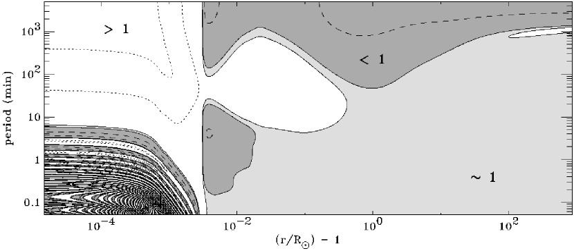
Figure 6: Contour/grayscale plot of the ratio $E_{K}/E_{B}$ as a function of height and wave period. The MHD-like regime of energy equipartition (i.e., a ratio of nearly 1) is shown in light gray, bounded by solid contours at values of 0.8 and 1.2. The kinetic-dominated regime is in white with dotted contours at values of $10^{2}$ and $10^{4}$. The magnetic-dominated regime is in dark gray with dashed contours at a value of 0.1.

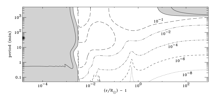
Figure 7: Contour/grayscale plot of the ratio $E_{+}/E_{-}$ as a function of height and wave period. The region of “strong” reflection is in gray, bounded by solid contours at values of 0.5 and 0.75. The location of the maximum value (0.99825) is denoted by a star. Other contours range between values of 10^-8 and 10^-1 and are labeled by their values. The transition region is clearly seen at $z\approx 0.003\,R_{\odot}$.

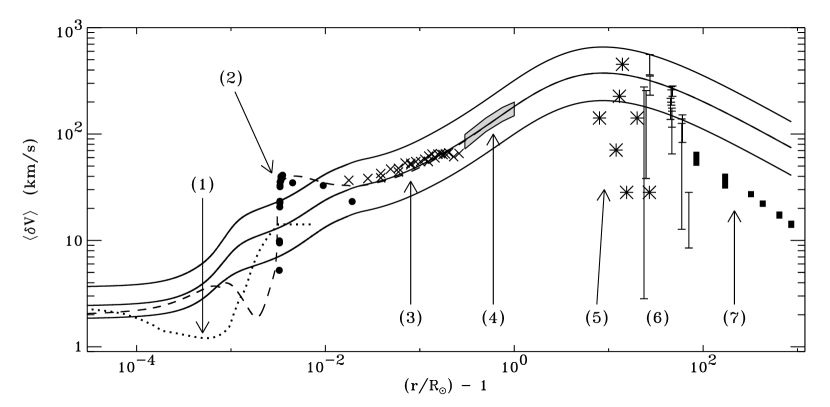
Figure 9: Height dependence of the frequency-integrated velocity amplitude. Solid lines give the undamped value of $\langle\delta V\rangle$ for three choices of $\sigma_{j}$: 0, 3, and 6 km s^-1 (from bottom to top). The dashed line is $\langle\delta V\rangle_{B}$ for the $\sigma_{j}=3$ km s^-1 case. Other lines and symbols correspond to observations discussed in detail in § 6.1.

The procedures outlined above resulted in a large amount of numerical data ($\sim$350 megabytes) describing the behavior of non-WKB kink-mode and Alfvén waves as a function of frequency and radius. In this section we attempt to distill and present the salient results in three gradual steps: (1) in Figures 5–7 we present frequency-dependent wave properties that have not yet been renormalized to the photospheric power spectrum (and thus are plotted as dimensionless ratios), (2) in Figure 8 we show the total power spectrum as a function of frequency for selected radii, and (3) in Figures 9–18 we present various frequency-integrated quantities that depend on the photospheric power normalization.

In order to determine to what degree the waves in various regions depart from ideal WKB theory, we show in Figure 5 the outward propagating wave action flux $f^{2}$ (defined in Appendix B) for a selection of periods, each normalized to the value of $f^{2}$ in the photosphere. For fluctuations having wavelengths so small that the local plasma parameters are approximately constant over several wavelengths, wave action is conserved and the quantity $f$ is constant. Note from Figure 5 that in the extended corona and solar wind (e.g., $z\gtrsim 1\,R_{\odot}$) Alfvén waves with periods shorter than a few hours obey wave action conservation, but for periods exceeding $\sim$10 hours this breaks down. Note that for all computed periods the wave action is not conserved below the transition region ($z\approx 0.003\,R_{\odot}$); this region acts as a sufficiently sharp “barrier” to induce significant reflection in the chromosphere (see also Wentzel 1978; Hollweg 1981; Campos & Gil 1999).

In much of the previous work on non-WKB Alfvén wave reflection, the departures from WKB theory have been characterized as a function of frequency. For frequencies exceeding a critical value $\omega_{A}$, the resulting wavelengths are so short that the wave propagates as if it were in a homogeneous medium and there is negligible reflection. For frequencies lower than $\omega_{A}$ there is significant reflection, and as $\omega\rightarrow 0$ the oscillation approaches the properties of a standing wave with equal inward and outward power. In a magnetized hydrostatic atmosphere, the critical frequency is given by the local value of $|\partial V_{A}/\partial r|$, or more precisely for arbitrary expansion factors, $|\nabla\cdot{\bf V}_{A}|$ (e.g., Ferraro & Plumpton 1958; An et al.  1990). In a supersonic wind, though, the radial dependence of the Alfvén speed is no longer the dominant factor in determining how much reflection takes place. At large distances from the Sun, Heinemann & Olbert (1980) and Barkhudarov (1991) showed that $\omega_{A}$ is given approximately by $u_{\infty}/2r_{A}$, where $u_{\infty}$ is the asymptotic outflow speed and $r_{A}$ is the Alfvén radius. (We use this expression as a fiducial definition of $\omega_{A}$, but we also note that it neglects several order-unity correction factors that depend on the flow tube geometry.) For the zero-order solar wind model defined in § 3.2 we find an associated critical period $2\pi/\omega_{A}$ of about 30 hours, or 1.25 days.

Figure 6 shows contours of the Alfvén ratio—i.e., the ratio of kinetic to magnetic energy density $E_{K}/E_{B}$ as a function of period and height. For ideal MHD Alfvén waves in a homogeneous medium this ratio is 1 and the waves are in energy equipartition (Walén 1944). Figure 6 can be broken up into four “quadrants” that have the following limiting properties:

1. Upper left: For long periods below the transition region, most of the wave energy is kinetic with only a negligible magnetic energy density. This is consistent with the predictions of kink-mode wave theory for the so-called “shallow” evanescent solution. In Appendix A we discuss several reasons why the solar atmosphere is suspected to naturally prefer this solution.

2. Lower left: For short periods below the transition region, the Alfvén ratio rapidly fluctuates above and below 1. This occurs because the wavelengths are small compared to the photospheric and chromospheric scale heights, but they are large compared to the scale heights in the transition region. Thus significant reflection occurred and there is a superposition of upward and downward waves. The fluctuations are well described by standing waves having fixed nodes in $v_{\perp}$ and $B_{\perp}$ (Hollweg 1981, 1984). If one could separate the solutions into the component upward and downward waves, their individual Alfvén ratios would be $\sim$1 as predicted by the kink-mode theory in Appendix A. (This can also be seen roughly by averaging over several nodes.)

3. Upper right: For long periods above the transition region, most of the wave energy is magnetic as was found by other non-WKB solar wind models (e.g., Heinemann & Olbert 1980). These long periods correspond to “quasi-static” motions of the field lines and have a similarity to the motions invoked in DC theories of coronal heating (e.g., Kuperus et al.  1981; van Ballegooijen 1986; Milano, Gómez, & Martens 1997).

4. Lower right: For short periods above the transition region, the plasma appears homogeneous to the relatively small-wavelength fluctuations and the ideal MHD equipartition holds.

Figure 7 shows contours of the ratio $E_{+}/E_{-}$ which can be thought of as an effective local reflection coefficient. The ideal WKB theory corresponds to a ratio of zero (i.e., all outward propagation). There is significant reflection below the transition region, with a maximum value of this ratio of 0.99825 at the photosphere for a period of $\sim$40 minutes. As discussed in § 5.2, we chose regularity conditions at the Alfvén critical point that ensured more outward than inward power at all heights, and thus $E_{+}/E_{-}$ must always be less than one. Below the transition region, the behavior of $E_{+}/E_{-}$ versus frequency resembles analytic solutions that take account of the chromospheric stratification and the strong reflection at the transition region (e.g., Hollweg 1978a; Schwartz, Cally, & Bel 1984). Because of the finite size of the atmosphere below the transition region, a mild resonance structure is seen in the amount of reflected wave flux (not apparent in Figure 7). The resonances are not as sharp as in the isothermal models of Schwartz et al.  (1984), though, because the nonzero temperature gradient results in a “smearing” of the preferred resonance frequencies.

Above the transition region, the solutions plotted in Figure 7 are very similar to those of Heinemann & Olbert (1980) and Barkhudarov (1991); there is significant reflection when $\omega\lesssim\omega_{A}$ and much less reflection for higher frequencies (lower periods). For frequencies above $\omega_{A}$—which we see below encompasses most of the dominant part of the power spectrum—we can use the analytic regularity conditions presented in § 4 of Barkhudarov (1991) to estimate the ratio $E_{+}/E_{-}$ at the Alfvén critical point:

$$\frac{E_{+}(\omega,r_{A})}{E_{-}(\omega,r_{A})}\,\approx\,\frac{1}{\omega^{2}}\left|\frac{\partial V_{A}}{\partial r}\right|_{r=r_{A}}^{2}\,\,\,\,\,\,\,\,\mbox{for}\,\,\omega\gg\omega_{A}\,\,\,.$$ (40)

By comparing to the numerical results in Figure 7 we verify that this relation is accurate for periods less than $\sim$200 minutes. It may be possible to also estimate the radial dependence of this ratio using similar analytic formulae. We defer this to future work, but note that this would be useful to models of coronal heating via turbulent cascade (see § 6.2.2).

Figure 8 shows the result of convolving the above results with the photospheric power spectrum derived in § 4. In this figure we plot the total power $P_{\rm tot}(\omega)$ for selected heights, and with a specific choice for the parameter $\sigma_{j}$ of 3 km s^-1 (see below). The amount of power loss between the photosphere and the merging height is consistent with the analytic predictions of isothermal kink-mode theory. For high frequencies (i.e., periods less than 3–5 minutes), $P_{\rm tot}$ decreases from $z=0$ to $z_{m}$ by a factor of 15 to 20; this is approximately the level of the decrease of the background magnetic field between those heights, implying that the propagating kink-mode relation $\rho v_{\perp}^{2}\propto B_{0}$ applies. For low frequencies (presumably evanescent), $P_{\rm tot}$ decreases by a factor of 190, which is very nearly equal to the drop in density from $z=0$ to $z_{m}$. This is consistent with the prediction of nearly constant $v_{\perp}$ for the shallow evanescent solution discussed in Appendix A (and thus $\rho v_{\perp}^{2}\propto\rho$). The somewhat irregular structure that develops in the spectrum between the photosphere and the merging height (and is passively advected outwards above $z_{m}$) is not numerical noise. Because of the nonisothermal temperature structure of the low chromosphere and the use of a radially varying filling factor $\phi$, the properties of the waves below the merging height depend on frequency in a more complicated way than in the ideal case described in Appendix A. If the upward and downward propagating waves had identical strengths and dispersive properties, the standing-wave nodes in $E_{K}$ and $E_{B}$ would cancel out exactly in $E_{\rm tot}$. However, $E_{\rm tot}$ exhibits a weak nodal structure because of incomplete cancellation and thus contributes to the irregularity in the power spectrum (see also Schwartz et al.  1984).

As in Figure 4, we plot in Figure 8 the product $\omega P_{\rm tot}$ versus wave period to more clearly show the periods that make the greatest contribution to the overall wave energy. We quantify this concept by defining the averaged, or first-moment frequency as

$$\langle\omega\rangle\,\equiv\,\frac{1}{U_{\rm tot}}\int_{0}^{\infty}d\omega\,\omega\,P_{\rm tot}(\omega)\,\,\,.$$ (41)

We plot this quantity versus height in Figure 14 below, but here we just note that the effective period $2\pi/\langle\omega\rangle$ is about 3.5 minutes in the photosphere, then it decreases to about 1.8 minutes above the merging height. Periods of a few minutes are natural to expect in the photosphere and chromosphere, and possibly in the corona as well (e.g., Chashei et al.  1999). However, it is reasonable to ask if these periods are expected to dominate in interplanetary space. In situ spacecraft generally measure fluctuations in velocity, density, and the magnetic field with the most power at periods of a few hours (e.g., Goldstein et al.  1995). However, a spacecraft sitting still in the ecliptic plane at 1 AU would see our model network flux tube rotate past in about 4 to 5 hours, with its component flux tubes (each originating in a different MBP) rotating by in substantially less than one hour. Thus it is possible that if the in situ power spectra actually do sample a “fossil” spectrum from the Sun, the dominant periods of order 1 hour could be due to the passage of many uncorrelated flux bundles past the spacecraft, and not the waves within any one flux bundle. (The ideal test would be to see if a spacecraft corotating with the solar rotation period measures a significantly different fluctuation spectrum than has already been observed.)

Figure 9, a key condensation of results for this paper, plots the frequency-integrated velocity amplitude $\langle\delta V\rangle$ as a function of height for a selection of $\sigma_{j}$ parameters and compares it to several different measurements of wave amplitudes. We discuss each set of measurements briefly, by number, below:

1. The dotted line shows a best-fit height dependence for the microturbulence needed to match photospheric and chromospheric line widths in the semiempirical VAL/FAL models (E.  Avrett, 2003, personal communication; see also Fontenla et al.  1993, 2002).

2. The filled circles show similar “nonthermal” line-broadening velocities measured (on the solar disk) in the transition region and low corona by the SUMER (Solar Ultraviolet Measurements of Emitted Radiation; Wilhelm et al.  1995) instrument on SOHO (the Solar and Heliospheric Observatory). The height of each point has been estimated by matching the height-dependence of temperature in the VAL/FAL model with the assumed formation temperatures of the ions that correspond to each point (Chae et al.  1998).

3. The crosses show nonthermal velocities inferred by SUMER measurements made above the solar limb (Banerjee et al.  1998). Off-limb Doppler broadening observations are better suited for measuring the properties of transverse Alfvén waves than observations on the solar disk.

4. The gray region shows lower and upper limits on the nonthermal velocity (Esser et al.  1999) as computed from off-limb measurements made by the UVCS (Ultraviolet Coronagraph Spectrometer) instrument on SOHO (Kohl et al.  1995, 1997).

5. The stars show early measurements (Armstrong & Woo 1981) of the random wavelike component of the solar wind velocity from interplanetary scintillation observations of radio signals passing through the corona, with the advecting diffraction pattern being measured by more than one receiver.

6. The error bars show a more recent determination of velocity fluctuations—specifically transverse to the radial direction—from radio scintillations (Canals et al.  2002) in the fast solar wind.

7. The Helios and Ulysses probes measured time-averaged Elsasser amplitudes that we converted to a representative velocity amplitude using eqs. (38)–(39) and assuming $U_{K}=U_{B}$ in the heliosphere. The data from both spacecraft were summarized by Bavassano, Pietropaolo, & Bruno (2000).

Measured line-of-sight (one-dimensional) velocities have been multiplied by $\sqrt{2}$ to take account of equivalent fluctuations in both transverse dimensions (e.g., eq. [9]).

Because measurements (1) and (2) above refer to motions mainly in the radial direction, we do not expect them to correspond to transverse kink-mode or Alfvén waves; they are plotted mainly for heuristic comparison. Note, though, that in Figure 9 we also plot (for the $\sigma_{j}=3$ km s^-1 case) a dashed curve that shows the frequency-averaged amplitude of the magnetic fluctuations in velocity units:

$$\langle\delta V\rangle_{B}\,\equiv\,\frac{\langle\delta B\rangle}{\sqrt{4\pi\rho}}$$ (42)

which for ideal MHD equipartition would be exactly equal to $\langle\delta V\rangle$. It is possibly a coincidence that this quantity so closely matches the Chae et al.  (1998) observations, but this agreement may contain information about the mode coupling between transverse and longitudinal waves in the transition region.

The three choices for the MBP-jump velocity amplitude $\sigma_{j}$ used in Figure 9 are 0, 3, and 6 km s^-1. The middle value seems to best match the off-limb nonthermal line broadening measurements, and we will use this as a baseline value in most subsequent calculations and plots. Note that the in situ measurements fall well below all of the reasonable choices for $\sigma_{j}$ (even the lower limit assuming no jumps whatsoever) and they exhibit a steeper gradient than the undamped models. The heliospheric “deficit” of wave power, compared to most prior assumptions about the wave power in the solar atmosphere, is well known (see, e.g., Roberts 1989; Lou 1993; Mancuso & Spangler 1999). In § 6.2.2 we propose a potential solution of these discrepancies based on a particular theory of turbulent wave damping in the solar wind.

Figure 10 shows additional details about the height dependence of the frequency-integrated wave properties. The ratio $U_{K}/U_{B}$ shows the region of strong departure from energy equipartition around the transition region, and that kinetic energy exceeds magnetic energy by a slight amount even down to the photosphere. The dimensionless magnetic amplitude $\langle\delta B\rangle/B_{0}$ is less then 1 over most of the computed range of heights (thus justifying the linear approximation), but exceeds 1 above $r\approx 19\,R_{\odot}$. Nonlinear calculations (e.g., Lau & Siregar 1996) find that $\langle\delta B\rangle/B_{0}$ does not grow so high in the heliosphere and may saturate at values close to 1.

Figure 11 shows the height dependence of the two Elsasser amplitudes. Above the transition region, the frequency-integrated outward propagating amplitude $\langle Z_{-}\rangle$ is much larger than the inward amplitude $\langle Z_{+}\rangle$. Below the transition region, the amplitudes approach a constant ratio $\langle Z_{-}\rangle/\langle Z_{+}\rangle\approx 1.027$. We also plot the height dependence of $Z_{-}$ that would be expected for ideal WKB wave action conservation (i.e., $f=\mbox{constant}$) and we scale it to the computed value of $\langle Z_{-}\rangle$ at 4 AU. The WKB value departs slightly from the non-WKB value between the transition region and a height of $\sim$0.01 $R_{\odot}$ and is substantially smaller below the transition region where there is strong inward wave power. The undamped linear curves all disagree markedly with the in situ measurements of the Elsasser amplitudes (see, however, § 6.2.2).

Lastly, in Figure 12 we plot the frequency-integrated energy flux density $F$ for the baseline $\sigma_{j}=3$ km s^-1 case. Below the merging height this quantity applies to the energy flux carried upward by the MBP kink modes, and above the merging height it applies to the volume-filling Alfvén waves. The wave flux is defined generally as

$$F\,\equiv\,u(U_{K}+2U_{B})+V_{A}(U_{-}-U_{+})\,\,,$$ (43)

which is based on the monochromatic definition given by Heinemann & Olbert (1980). For outward propagating waves obeying wave action conservation, one can write $F=U_{\rm tot}(1.5u+V_{A})$. In the lowest layers of the atmosphere one can also ignore the factors above that depend on $u$ and thus the net flux depends mainly on the difference between $U_{-}$ and $U_{+}$. Because of the strong reflection below the transition region there is strong cancellation; i.e., the magnitude of the purely outward wave flux $V_{A}U_{-}$ exceeds the net flux by a factor of about 20. This means that $\sim$95% of the kink-mode wave energy below the transition region is “trapped,” with only 5% escaping.

Analysis of a series of models having a range of $\sigma_{j}$ values yields a potentially useful explicit expression for the photospheric wave flux in the MBPs. Recalling that the random-walk and impulsive parts of the power spectrum are assumed to be linearly independent (e.g., eq. [16]), we have fit the numerically computed photospheric fluxes with the following function:

$$\frac{F_{\odot}}{10^{7}\,\mbox{erg}\,\mbox{cm}^{-2}\,\mbox{s}^{-1}}\,\approx\,9.75\,+\,2.48\left(\frac{\sigma_{j}}{1\,\mbox{km}\,\mbox{s}^{-1}}\right)^{2}$$ (44)

with less than 0.1% uncertainty in the fit (mainly due to roundoff error in the above expression having only three significant figures). Thus, for the reasonable range of $\sigma_{j}$ between 0 and 6 km s^-1, $F_{\odot}$ ranges between about 10⁸ and 10⁹ erg cm^-2 s^-1 (see also Musielak & Ulmschneider 2001). Note that for any given value of $\sigma_{j}$ the jump-term in the above expression has a greater relative contribution to the total flux than the corresponding jump-term in eq. (16) has to the photospheric velocity variance. This occurs because the bulk of the power in the jump motions is at higher frequencies than the walk motions and is less susceptible to evanescent decay. The flux is a frequency-integrated quantity that incorporates this aspect of the solutions, whereas the velocity variance does not.

We also plot in Figure 12 several other flux quantities. The “granule-averaged” wave flux is given by the quantity $\phi F$ (for the flux tube filling factor $\phi$, see eq. [30]), and it differs from $F$ itself only below the merging height. The quantity $\phi F$ spreads the wave energy out evenly within the modeled network patch, and thus is a more relevant quantity to compare with observations and predictions of wave fluxes that arise in the network from the convection. Note that the photospheric value of $\phi F=2.7\times 10^{7}$ erg cm^-2 s^-1 is of similar magnitude as the acoustic wave flux of $5\times 10^{7}$ erg cm^-2 s^-1 predicted by Musielak et al.  (1994). We also plot a “supergranule-averaged” flux $\phi_{c}F$, where $\phi_{c}$ is a filling factor for the large-scale funnel/canopy magnetic structure shown in Figure 2. (We define $\phi_{c}$ only below the top height [12 Mm] of the magnetostatic grid, as the ratio of the field strength at that top height [11.8 G] to the field strength along the central axis of the flux tube at lower heights.) The quantity $\phi_{c}F$ is what one would use in order to compute the total wave power (in erg s^-1) integrated over the entire coronal hole.

6.2 Wave Dissipation

In this section we discuss two separate mechanisms that have been proposed to damp Alfvén waves in the solar atmosphere and solar wind: viscosity (§ 6.2.1) and MHD turbulent cascade (§ 6.2.2). For clarity we do not treat these mechanisms together, though in a completely self-consistent model all damping mechanisms should be included and allowed to interact with one another.

6.2.1 Linear Viscous Dissipation

The first damping mechanisms proposed for MHD waves in the solar corona were collisional in nature (Alfvén 1947; Osterbrock 1961). In the high-density plasma near the Sun, MHD waves can be damped by viscosity, thermal conductivity, electrical resistivity (i.e., Joule/Ohmic heating), and ion-neutral friction. For Alfvén and fast-mode waves propagating parallel to the magnetic field, though, the dominant collisional dissipation channel in the corona is believed to be proton viscosity. Here we estimate the viscous damping expected for the background plasma conditions described above and find it to be negligible.

We compute a collisional damping length $L_{c}$ as a function of height $z$, and there should be appreciable damping only where $L_{c}\lesssim z$. Generally, the product of the damping length and a linear damping rate $\gamma$ (i.e., the imaginary part of the frequency) is the wave group velocity $V_{\rm gr}$ in the inertial frame, given here for dispersionless Alfvén waves as $u+V_{A}$. For viscous damping, $\gamma=\nu_{p}k^{2}$, where $\nu_{p}$ is the proton kinematic viscosity and $k$ is the radial wavenumber (van de Hulst 1951; Osterbrock 1961). Thus, for Alfvén waves propagating upward and parallel to the background magnetic field, this leads to the general expression

$$L_{c}\,\approx\,\frac{(u+V_{A})^{3}}{\nu_{p}\omega^{2}}$$ (45)

(Tu 1984; Whang 1980, 1997). In a strongly collisional plasma the kinematic viscosity is given by the classical Braginskii (1965) formalism (see also Hollweg 1986a). In the collisionless solar wind, though, there is no clear prescription for the effective viscosity. We thus define the proton kinematic viscosity phenomenologically as

$$\nu_{p}\,=\,w_{p}^{2}\tau_{\rm eff}\,=\,\frac{k_{\rm B}T_{p}\tau_{\rm eff}}{m_{p}}$$ (46)

where $w_{p}$ is the proton most-probable speed, $k_{B}$ is Boltzmann’s constant, $T_{p}$ is the proton temperature, $m_{p}$ is the proton mass, and $\tau_{\rm eff}$ is an effective viscous timescale. We adopt a fiducial proton temperature law for this analysis that comes from the semiempirical VAL/FAL model (used for the magnetostatic flux tube model) below $x=1.0172$, and we use

$$T_{p}\,=\,\frac{5\times 10^{5}\,\mbox{K}}{0.2+0.02x^{0.8}+0.21x^{-33}}$$ (47)

above 1.0172 $R_{\odot}$. This expression reasonably reproduces the proton temperatures measured by Helios and Ulysses in the highest-speed solar wind (Tu, Freeman & Lopez 1989; Goldstein et al.  1996) and it has a peak in the extended corona of $\sim$2.2 MK in general agreement with UVCS/SOHO H I Ly$\alpha$ measurements (e.g., Kohl et al.  1998; Esser et al.  1999).

For strong collisional coupling, the effective viscous time scale $\tau_{\rm eff}$ is given by the mean time between collisions (Braginskii 1965),

$$\tau_{\rm coll}\,=\,\frac{3}{4}\sqrt{\frac{m_{p}}{\pi}}\frac{(k_{\rm B}T_{p})^{3/2}}{n_{\rm H}\,e^{4}\ln\Lambda_{c}}$$ (48)

where $e$ is the proton/electron charge and $\ln\Lambda_{c}$ is the Coulomb logarithm, taken here to be 21. The above timescale applies to the viscous damping of motions along the magnetic field. For shear motions transverse to the field, though, the appropriate viscous time (even in the limit of strong collisions) is reduced. The off-diagonal Braginskii coefficients in the stress tensor are obtained approximately by dividing $\tau_{\rm coll}$ by dimensionless factors that take account of the magnetic field. Thus,

$$\tau_{\rm eff}\,\approx\,\frac{\tau_{\rm coll}}{(\Omega_{p}\tau_{\rm coll})^{m}}\,\,,$$ (49)

where $m$ is either 1 or 2, and $\Omega_{p}$ is the proton Larmor frequency $eB_{0}/m_{p}c$. The $m=0,1,2$ terms are roughly analogous to the direct, Hall, and Pedersen components of the MHD conductivity in an ionized plasma.

In the low-density collisionless limit, the classical $m=0$ case cannot apply because it would imply the viscosity becomes infinitely large as the mean time between collisions becomes infinite (the “molasses” limit). Williams (1995) argued essentially that the general viscosity in a collisional or collisionless plasma is found by taking the shorter of either the $m=0$ or the $m=1$ timescales. We assert, though, that the $m=2$ case seems to be the most appropriate for the viscous damping of transverse Alfvén waves in the collisionless solar wind. Consider the viscosity as an effective diffusion coefficient ($\ell^{2}/t$) describing scattering events with mean-free-path length and time scales of $\ell$ and $t$, respectively. The actual energy losses arise from the interparticle collisions with timescale $t\approx\tau_{\rm coll}$, but spatially the transverse structure would be dominated by features with sizes of order the proton thermal Larmor radius, and thus $\ell\approx w_{p}/\Omega_{p}$. For these values the viscosity reproduces the $m=2$ case.

Figure 13 shows the radial dependence of the linear damping length $L_{c}$ for the three cases, $m=0$, 1, and 2, computed for a wave period of 1 minute. For heights below about 0.3 $R_{\odot}$ above the photosphere, it is unlikely that any damping would take place because all three cases have damping lengths much longer than the local height. This mid-corona distance ($r\approx 1.3$ to 2 $R_{\odot}$) is approximately where collisions start to become unimportant in coupling together electron, proton, and heavy ion plasma properties (e.g., Cranmer, Field, & Kohl 1999). Above this height, then, the appropriate damping length should transition to either the $m=1$ or the $m=2$ case, both of which are substantially longer than the local height in the corona. In the far solar wind, we believe the $m=2$ case is the most realistic, and it always remains several orders of magnitude larger than the local height. Thus, our preliminary conclusion is that for both waves near the peak of the power spectrum (periods of a one to a few minutes), and for longer periods, linear viscous damping is unimportant as a significant attenuation mechanism for Alfvén waves in the corona and fast solar wind. For periods much shorter than 1 minute, though, this kind of damping could be important—and may have already been responsible for the sharp drop in power inferred from photospheric MBP motions between 0.1 and 1 minute.

6.2.2 Nonlinear Turbulent Dissipation

The second type of wave damping we consider is turbulent dissipation; i.e., a nonlinear cascade of energy from large to small scales that terminates in an irreversible conversion of wave energy into heat. The need to include some kind of nonlinear damping or saturation can be seen in Figure 10, where above a distance of $\sim$20 $R_{\odot}$ the magnetic fluctuation amplitude begins to exceed the background field strength (in opposition to in situ observations) and the linear assumption breaks down. Addressing the full problem of anisotropic MHD turbulence in the solar corona and solar wind, though, is well beyond the scope of this paper (see, though, Cranmer & van Ballegooijen 2003 for a summary of many related issues). Here we include only one specific aspect of this theory: a phenomenological damping rate that depends on the properties of the largest scales in the turbulence and not on the details of the cascade.

The presence of both outward and inward propagating Alfvén waves is a necessary prerequisite for the nonlinear coupling to higher wavenumber that drives the cascade (see, e.g., Matthaeus et al.  1999; Dmitruk, Milano, & Matthaeus 2001). Any expression for the turbulent energy decay must then depend on both the $z_{-}$ and $z_{+}$ Elsasser amplitudes, and thus the inclusion of turbulence introduces further coupling between these two modes. A straightforward phenomenological form for the nonlinear transport has been suggested by Zhou & Matthaeus (1990) from the standpoint of “reduced MHD” (RMHD; see also Strauss 1976; Montgomery 1982). Effectively, the transport equation is the same as eq. (32), but with the following term added to the right-hand side:

$$-\frac{z_{\pm}|z_{\mp}|}{2L_{\perp}}$$ (50)

where $L_{\perp}$ is a transverse length scale representing an effective correlation length of the turbulence—i.e., a similarity length scale associated with the energy transport from large to small eddies. (It may be imprecise to refer to this length scale as an “outer scale,” but for simplicity we treat this as a synonym.) We assume that $L_{\perp}$ scales with the transverse width of the open flux tube; i.e., that it remains proportional to $B_{0}^{-1/2}$. Specifically, we normalize $L_{\perp}$ by specifying its value at the merging height $z_{m}$. We also define the constant $\Lambda$ as the ratio of $L_{\perp}$ at the merging height to the transverse radius of the network flux bundle at that height: 3 Mm (see Figure 2). Equivalently, we can express

$$L_{\perp}(r)\,\approx\,\frac{33\,\Lambda}{\sqrt{B_{0}(r)}}\,\,\mbox{Mm}$$ (51)

if $B_{0}$ is measured in Gauss (see also Hollweg 1986b).

In order to know how best to implement the nonlinear term given above, we need to understand over what range of heights this term acts to appreciably damp the waves. We do not expect a strong RMHD cascade to develop in the region below the merging height because—despite the stochastic nature of the fluctuation spectrum—the flux tubes do not strongly interact with one another. For heights above $z_{m}$ we can compare the effective damping length $L_{\perp}$ to the local height $z$ above the photosphere. For $\Lambda=1$, we find that $L_{\perp}<z$ only above a height of $z\approx 0.01\,R_{\odot}$. It makes sense that the chromosphere and transition region are not expected to undergo much damping from this RMHD mechanism; there seems to be insufficient time for the turbulent cascade to develop in such small volumes. Dmitruk & Matthaeus (2003) discussed a hierarchy of timescales that should be satisfied in order for this turbulent damping process to be strong. A simplified version of this hierarchy is as follows:

$$t_{0}\,<\,t_{R}\,<\,t_{f}\,\,\,,$$ (52)

where $t_{0}$ is a nonlinear outer-scale eddy cascade time, $t_{R}$ is a timescale for Alfvén wave reflection, and $t_{f}$ is representative of the main driving period of the waves. In Figure 14 we compare several of these quantities to see where these conditions are met.

In Figure 14 we plot a representative reflection time $t_{R}$ which we define as $1/|\nabla\cdot{\bf V}_{A}|$. This is probably of the same order of magnitude as the Dmitruk & Matthaeus (2003) “Alfvén wave crossing time” $t_{A}$, since the latter can be defined as $H_{A}/V_{A}$, or the wave travel time over a representative Alfvén-speed scale height $H_{A}$. Thus, $t_{R}\approx t_{A}$. For reference we also show the total wave travel time from the photosphere to a given height, defined as

$$t_{\rm trav}(r)\,\equiv\,\int_{R_{\odot}}^{r}\frac{dr^{\prime}}{u(r^{\prime})+V_{\rm ph}(r^{\prime})}\,\,\,.$$ (53)

We equate the driving period $t_{f}$ to the spectrum-integrated first-moment period $2\pi/\langle\omega\rangle$ (see eq. [41]) and we plot its value for the baseline $\sigma_{j}=3$ km s^-1 model. Interestingly, $t_{f}>t_{R}$ only below $z\approx 0.5\,R_{\odot}$, and the hierarchy is not satisfied at large distances where the damping length is relatively small. Note, though, that the demand in the above hierarchy for $t_{f}$ to be the largest of the three timescales comes only from the well-known non-WKB result that long periods are the easiest to reflect, and thus they provide the most turbulent mixing between inward and outward modes. However, the amount of reflection in our model is a known quantity (see, e.g., Figures 7 and 11), and it is irrelevant whether it could have been maximized with longer-period waves. Therefore we do not need to consider the last inequality in eq. (52) as a precondition for turbulent damping.

The key piece of the Dmitruk & Matthaeus (2003) timescale hierarchy is that the nonlinear driving time $t_{0}$ must be short compared to the reflection time $t_{R}$. Only when this condition is satisfied can the turbulent cascade develop to the point where the wave damping can occur efficiently. In Appendix C we describe one way of using a model for the anisotropic turbulent power spectrum to derive $t_{0}$ (see also Oughton, Dmitruk, & Matthaeus 2004). This timescale depends inversely on the outer-scale length $L_{\perp}$, and in Figure 14 we plot the radial dependence of $t_{0}$ for two extreme values of the normalizing constant $\Lambda$. An upper limit to the outer-scale length is given by $\Lambda=1$ (i.e., that the “stirring” takes place on the spatial scale of the entire network element). A reasonable lower limit for $L_{\perp}$ at the merging height is the radius of the smallest expected MBP flux tube. At the merging height, the flux tubes have expanded to fill the volume of the network patch, and thus the MBP radius is given by half the nearest-neighbor distance $d_{nn}$. For the lower-limit value of $d_{nn}\approx 350$ km (see § 3.1) we obtain a lower limit of $\Lambda=0.06$.

We find in Figure 14 that $t_{R}$ begins to exceed $t_{0}$ somewhere above a height of 0.1 to 1 $R_{\odot}$. We thus solve the nonlinearly modified wave transport equation only above 0.1 $R_{\odot}$. This restriction allows us to make a useful simplifying assumption. As seen in Figure 11, above this height there is only relatively weak inward wave power; i.e., $\langle Z_{-}\rangle\gg\langle Z_{+}\rangle$. We solve a modified time-steady wave action conservation equation in the limit of pure outward propagation. Note also that turbulence does not act in a straightforward “monochromatic” way, as was assumed in the constant-frequency linear solutions to eq. (32). We thus ignore any frequency (and wavenumber) transport and compute the overall effects of the turbulent damping on the frequency-integrated wave energy (see, however, Verdini & Velli 2003). Thus, we solve the following modified spectrum-averaged wave action conservation equation in the limits of no time dependence and dominant outward propagation:

$$\frac{uV_{A}}{u+V_{A}}\frac{\partial}{\partial r}\left[\frac{(u+V_{A})^{2}\langle Z_{-}\rangle^{2}}{uV_{A}}\right]\,=\,-\frac{\langle Z_{-}\rangle^{2}\langle Z_{+}\rangle}{L_{\perp}}$$ (54)

(see Appendix B). We use the linear solution for $\langle Z_{+}\rangle$ obtained above in order to solve for the nonlinearly damped value of $\langle Z_{-}\rangle$:

$$\frac{\langle Z_{-}\rangle^{2}}{\langle Z_{-}\rangle_{0}^{2}}\,=\,\frac{(u_{0}+V_{A,0})^{2}\,uV_{A}}{(u+V_{A})^{2}\,u_{0}V_{A,0}}\,\exp\left\{-\int_{r_{0}}^{r}\frac{dr^{\prime}\,\langle Z_{+}(r^{\prime})\rangle}{[u(r^{\prime})+V_{A}(r^{\prime})]L_{\perp}(r^{\prime})}\right\}\,\,,$$ (55)

where all quantities with subscript ‘0’ are given at the effective lower boundary $z=0.1\,R_{\odot}$. This is not a completely self-consistent method of obtaining the damped wave power, since no back-reaction on $\langle Z_{+}\rangle$ is computed, but it gives an adequate order-of-magnitude result for the total power in the regions dominated by outward propagating waves.

Figure 15 shows the result of integrating eq. (55) for three choices of $\Lambda$ (0.1, 0.35, and 1), as well as the solution for no damping ($\Lambda\rightarrow\infty$). We plot these solutions as velocity amplitudes in order to facilitate comparison with the observational data, which are also plotted as in Figure 9. For each value of $\Lambda$, the resulting damped $U_{-}$ energy density was added to $U_{+}$ (which remains undamped) to obtain $U_{\rm tot}$, and this total energy density was split into kinetic and magnetic parts assuming that the linear undamped ratio $U_{K}/U_{B}$ remains the same for the damped models. The resulting $U_{K}$ was then used to compute $\langle\delta V\rangle$ as in eq. (38).

The value of $\Lambda$ that produces the best agreement with the in situ measurements is approximately 0.35, implying a transverse outer scale at the merging height of about 1100 km. This value seems appropriate and consistent for motions excited between granules of the same spatial scale. If $\Lambda$ were much smaller than this value, it would imply that the turbulence was dominated by internal motions in the MBP flux tubes, which we essentially ignore in the thin-tube models. Furthermore, note from Figure 15 that for $\Lambda\leq 0.1$ there is so much damping that the approximation $\langle Z_{-}\rangle\gg\langle Z_{+}\rangle$ breaks down above $\sim$100 $R_{\odot}$ and we would have needed to solve a more complicated set of damping equations. The observational constraints which imply $\Lambda=0.35$ allow us to avoid both of the above consistency problems that arise for smaller values.

Properties of the $\Lambda=0.35$ solutions were also plotted in several other figures in order to compare with the linear results. Figure 10 shows that the damped magnetic amplitude ratio $\langle\delta B\rangle/B_{0}$ is smaller in interplanetary space than the undamped ratio. For the damped model, $\langle\delta B\rangle/B_{0}$ exceeds 1 only above 135 $R_{\odot}$ and does not exceed a value of 1.7 within the computed range of distances (see also Lau & Sireger 1996). Figure 11 shows the better agreement between the damped Elsasser amplitude $\langle Z_{-}\rangle$ and the measured outward Elsasser energy. The inward amplitude $\langle Z_{+}\rangle$ still does not agree with the measured inward Elsasser energy (see also Hollweg 1990), but note that the linear value was not modified in the damping calculations done here. Full simulations of the turbulence would probably see an enhancement of $\langle Z_{+}\rangle$ and possibly even an approach to inward/outward energy equipartition (e.g., Oughton & Matthaeus 1995).

6.3 Impact on the Steady-State Plasma

A self-consistent treatment of waves in the solar atmosphere and solar wind would consider the impact of fluctuations on the mean, time-steady plasma properties. Incorporating this back-reaction into the model steady state is beyond the scope of this paper, but below we compute a subset of the necessary source terms (e.g., the heating rate and the wave pressure acceleration) for use in future models.

6.3.1 Heating due to Turbulent Dissipation

The nonlinear wave damping discussed in § 6.2.2 produces gradual heat deposition along an open magnetic flux tube. The rate of energy conversion is derivable essentially from eq. (54), and here we give a slightly more general version of the energy conversion rate based on a comparison between phenomenological turbulence models and numerical simulations. The time rate of change in the general Elsasser variance $\langle Z_{\pm}\rangle^{2}$ is given by

$$\frac{d\langle Z_{\pm}\rangle^{2}}{dt}\,=\,-\alpha_{\pm}\frac{\langle Z_{\pm}\rangle^{2}\langle Z_{\mp}\rangle}{L_{\perp}}$$ (56)

(e.g., Hossain et al.  1995; Matthaeus et al.  1999; Dmitruk et al. 2001, 2002). Comparison with numerical simulations found that the dimensionless parameter $\alpha_{\pm}$ is of order unity. We thus assume $\alpha_{\pm}=1$ and define the total heating rate $Q$ as

$$Q\,\equiv\,-\frac{dU_{\rm tot}}{dt}=\,\rho\,\frac{\langle Z_{-}\rangle^{2}\langle Z_{+}\rangle+\langle Z_{+}\rangle^{2}\langle Z_{-}\rangle}{4L_{\perp}}\,\,\,.$$ (57)

In our models this quantity is defined consistently only above $z=0.1\,R_{\odot}$, where the damping is applied, but below we calculate $Q$ for all heights along the flux tube. We caution that the heating rates below 0.1 $R_{\odot}$ are only estimates based on the undamped Elsasser amplitudes at those heights.

Figure 16 plots the heating rate per unit mass ($Q/\rho$) for the range of $\Lambda$ values shown in Figure 15 in addition to an even weaker-damping case of $\Lambda=3$. For the regions where the nonlinear damping does not change the radial profiles of $\langle Z_{\pm}\rangle$ from their undamped values, $Q$ scales with $\Lambda^{-1}$ as expected. However, for heights where damping occurs the heating rate is lowered because of the cumulative loss of wave power up to that height. Thus, for each height, there is a maximum heating rate that defines a critical value $\Lambda_{\rm crit}$. For $\Lambda>\Lambda_{\rm crit}$ the cumulative damping grows weaker, and the decrease in $Q$ comes from the increase in the denominator of eq. (57). For $\Lambda<\Lambda_{\rm crit}$, there is more cumulative damping and the decrease in $Q$ comes from the loss of local wave power in the numerator of eq. (57). For a distance of $r=2\,R_{\odot}$ in the extended corona, $\Lambda_{\rm crit}$ is about 0.07, and the maximum heating rate per unit mass at that value is $\sim 3.9\times 10^{11}$ erg s^-1 g^-1.

We also plot in Figure 16 an empirical heating rate (summed from proton and electron contributions) that was derived in order to reproduce a large number of remote-sensing and in situ measurements of fast solar wind conditions. We use the heating rates from the SW2 model of Allen, Habbal, & Hu (1998). For comparison with the above numbers, the empirically constrained heating rate at $r=2\,R_{\odot}$ is about $1.2\times 10^{11}$ erg s^-1 g^-1 (see also Dmitruk et al.  2002; Cranmer 2002). In the extended corona ($r\approx 2$–3 $R_{\odot}$), Figure 16 shows that the empirical heating rate agrees best with the $\Lambda=0.35$ case that also produces the right amount of in situ damping (Figure 15). This rough agreement provides additional support for the outer-scale normalization specified by this value.

It is worthwhile also to compare the heating rates computed above with those computed using a damping rate appropriate for isotropic Kolmogorov (1941) turbulence (see, e.g., Hollweg 1986b; Chae et al.  1998; Li et al.  1999; Chen & Hu 2001). In order to derive a Kolmogorov heating rate appropriate for quantitative comparison with the above results, we make both the quasi-isotropic approximation $U_{-}=U_{+}$ and we assume MHD energy equipartition $U_{K}=U_{B}$. Thus, eq. (57) becomes

$$Q_{\rm kol}\,=\,\frac{\rho\,\langle\delta V\rangle^{3}\,\sqrt{2}}{L_{\perp}}$$ (58)

where we use the damped velocity amplitude $\langle\delta V\rangle$ as plotted in Figure 15. The above expression differs by a factor of $\sqrt{2}$ from the simpler formulae given in many other papers; this factor is required in order to remain consistent with the isotropic/equipartition limit of eq. (57). Removing this factor would be equivalent to specifying $\alpha_{\pm}=1/\sqrt{2}$ in eq. (56), but we note that the relative comparison between eqs. (57) and (58) does not depend on the value of $\alpha_{\pm}$.

In Figure 17 we plot the comparison between the complete heating rate $Q$ and the Kolmogorov approximation $Q_{\rm kol}$. For simplicity we show only the case having the preferred $\Lambda=0.35$ outer-scale normalization. The curves are substantially different from one another nearly everywhere, which indicates that the inward/outward imbalance generated by non-WKB reflection is probably a very important ingredient in Alfvén wave heating models of the solar wind. The differences are small in the photosphere and low chromosphere, where strong reflection leads to nearly equal inward and outward wave power. In the extended corona, though, the Kolmogorov heating rate begins to exceed the anisotropic turbulent heating rate by as much as a factor of 30. The isotropic Kolmogorov assumption assumes the maximal amount of possible mixing between inward and outward modes, which is inconsistent with the relatively weak reflection computed for the corona in our models.

Figure 17 also shows the radial dependence of an analytic scaling relation for the turbulent heating rate given by Dmitruk et al.  (2002) for the region above the coronal maximum in $V_{A}$. This scaling relation gives $Q\propto B_{0}|\partial V_{A}/\partial r|$, and we show it for an arbitrary normalization. The analytic heating rate per unit mass has a radial gradient less steep than the other curves in Figure 17, but it has a general shape that is similar.

6.3.2 Wave Pressure Acceleration

Waves that propagate radially through an inhomogeneous medium exert a nondissipative net force on the gas. This net momentum deposition has been studied for several decades for both acoustic and MHD waves and is generally called either “wave pressure” or the ponderomotive force (e.g., Bretherton and Garrett 1968; Dewar 1970; Belcher 1971; Alazraki and Couturier 1971; Jacques 1977). Initial computations of the net work done on the bulk fluid have been augmented by calculations of the acceleration imparted to individual ion species (e.g., Isenberg & Hollweg 1982; McKenzie 1994; Li et al.  1999), estimates of the departures from Maxwellian velocity distributions induced by the waves (Goodrich 1978; Hollweg 1978b), and extensions to nonlinearly steepened wave trains (Gail, Ulmschneider, & Cuntz 1990; Pijpers 1995).

For non-WKB Alfvén waves propagating in a radial flux tube, Heinemann & Olbert (1980) gave the general second-order expression for the wave pressure acceleration:

$${\bf a}_{\rm wp}\,=\,-({\bf v}_{\perp}\cdot\nabla){\bf v}_{\perp}+\frac{1}{4\pi\rho}\left[(\nabla\times{\bf B}_{\perp})\times{\bf B}_{\perp}\right]$$ (59)

which has the radial component

$$a_{\rm wp}\,=\,-\frac{1}{8\pi\rho}\frac{\partial|B_{\perp}|^{2}}{\partial r}\,+\,\left(\frac{|B_{\perp}|^{2}}{8\pi\rho}-\frac{|v_{\perp}|^{2}}{2}\right)\frac{\partial}{\partial r}(\ln B_{0})\,\,.$$ (60)

In the limit of equipartition between the kinetic and magnetic wave energy densities, the term in parentheses is zero. For a spherical geometry (e.g., MacGregor & Charbonneau 1994), we note that the quantity $\partial(\ln B_{0})/\partial r$ can be written simply as $-2/r$.

In our non-WKB model we have computed the frequency-integrated kinetic and magnetic energy densities $U_{K}$ and $U_{B}$. We find that the spectrum-weighted wave pressure acceleration can be expressed in terms of these variables as

$$\rho\langle a_{\rm wp}\rangle\,=\,-\frac{\partial U_{B}}{\partial r}+\left(U_{B}-U_{K}\right)\frac{\partial}{\partial r}(\ln B_{0})\,\,\,.$$ (61)

Figure 18 compares the computed values of $\langle a_{\rm wp}\rangle$ for the undamped ($\sigma_{j}=3$ km s^-1) and damped ($\Lambda=0.35$) cases, as well as an effective WKB wave pressure computed using just the first term on the right-hand side of eq. (61). There is some numerical noise in the plots that comes from the necessity to take numerical derivatives. Departures from the idealized WKB form arise only below $z\approx 0.03\,R_{\odot}$ and thus may not be important for the acceleration of the solar wind. In the photosphere, though, the non-WKB wave pressure acceleration exceeds the approximate WKB acceleration by a factor of 100. The WKB approximation also gives an unrealistically large spike in $\langle a_{\rm wp}\rangle$ at the transition region that does not appear in the exact non-WKB solution. It remains to be seen if these differences would significantly affect various observational constraints placed on the properties of the transition region (e.g., Woods, Holzer, & MacGregor 1990a, 1990b).

Figure 18 also shows the magnitude of the Sun’s gravitational acceleration $g$ as a function of height. Presumably, the wave pressure acceleration has little net effect on the corona and solar wind in regions where $|\langle a_{\rm wp}\rangle|\ll g$. For closed coronal loops, though, Laming (2004) computed a similar non-WKB wave pressure acceleration and found that its strength can rival that of gravity even in the chromosphere. The Alfvén wave reflection in these models is strong enough to produce ion abundance variations that may explain the observed dependence on First Ionization Potential (FIP).

7 Summary of Major Results

The goal of this work was to produce a detailed and self-consistent description of the global energy budget of transverse incompressible waves in open magnetic regions of the solar atmosphere. Here we list the unique features of the model, key results, and some of the insights gained about the overall wave-plasma system.

1. Measurements of G-band bright points in the photosphere were used to set the power spectrum of transverse waves as the lower boundary condition of our model. The observationally inferred power spectrum was summed from two phases of MBP motion assumed to be statistically independent: isolated random walks and occasional rapid jumps due to MBP merging, fragmenting, or magnetic reconnection.

2. The steady-state plasma density, magnetic field, and flow velocity were constrained empirically from the photosphere to a distance of 4 AU. The successive merging of flux tubes on granular and supergranular scales in the atmosphere was described using a two-dimensional magnetostatic model of the magnetic network element.

3. Non-WKB wave transport equations, incorporating linear reflection terms, were solved for a grid of wave periods between 3 and $3\times 10^{5}$ s over the range of heights given above. Below a mid-chromospheric merging height the waves were modeled as modified kink-mode flux tube waves, and above this height they were modeled as Alfvén waves propagating parallel to the background magnetic field.

4. The waves are reflected strongly at the transition region, with only about 5% of the wave energy transmitted and 95% reflected. Above the transition region, most periods are reflected only weakly by the large-scale radial gradient of the Alfvén speed, but periods exceeding 1 day are reflected strongly in interplanetary space. The period-averaged reflection coefficient from the extended corona ($r=2\,R_{\odot}$) to 1 AU ranges between $10^{-4}$ and $10^{-3}$.

5. At the photosphere, the wave periods containing the most power are between 1 and 30 minutes, but the kink-mode waves with periods greater than about 12 minutes are evanescent below the merging height. Only the shorter periods propagate to larger distances, and above the merging height the power spectrum is dominated by wave periods between about 1 and 6 minutes. In situ observations of power spectra that are strongest at periods of several hours may be explained by many uncorrelated flux tubes rotating past spacecraft in the solar wind on these longer timescales.

6. The period-averaged transverse velocity amplitude of the waves agrees with observed off-limb nonthermal line widths from SUMER and UVCS when the MBP jump amplitude $\sigma_{j}$ is taken to be $\sim$3 km s^-1. For all reasonable values of $\sigma_{j}$ between 0 and 6 km s^-1 the modeled wave amplitudes at heights greater than 0.3 AU are significantly larger than the in situ measurements, implying that large-scale damping is needed.

7. We investigated the potential impact of the linear viscous damping of Alfvén waves. If the effective viscous stress timescale undergoes a transition from its collisionally dominated form to either of the possible collisionless forms (given by the $m=1$ or 2 cases of § 6.2.1), the resulting damping lengths are always much longer than the local height from the photosphere, and viscosity thus cannot damp the waves.

8. We also considered nonlinear turbulent damping using a phenomenological model of the energy loss terms in the wave transport equations. The one free parameter is the normalization of the outer-scale correlation length $L_{\perp}$ of the turbulence, which scales with height as $B_{0}^{-1/2}$. Interestingly, a single choice for the constant $\Lambda=0.35$, which specifies the value of $L_{\perp}$ at the merging height to be about 1100 km, produces both the right amount of damping above 0.3 AU to agree with the in situ measurements and the right amount of heating in the extended corona to agree with empirically constrained solar wind acceleration models.

9. Because of the relatively weak degree of reflection in the corona, non-WKB effects are probably not important for computing the wave pressure acceleration in regions that contribute to the overall solar wind acceleration. However, non-WKB effects produce order-of-magnitude differences (from the WKB approximation) in the wave pressure acceleration at and below the transition region. The inclusion of damping also affects the total amount of wave pressure acceleration imparted to the solar wind.

8 Discussion

The model presented in this paper contains a great deal of the relevant physics of Alfvén waves in the solar atmosphere and solar wind, but it is incomplete in several ways. In this section we discuss various ways to extend the model to improve its physical realism.

Our cylindrically symmetric magnetostatic model of the network flux tube is highly idealized. A fully three-dimensional model of a network “patch,” possibly using a high-resolution magnetogram image as the lower boundary condition, would have a more realistic geometry (see, e.g., van Ballegooijen & Hasan 2003). Such a model would contain a distribution of flux tube strengths, merging heights, and canopy heights. The resonant node structure seen in the power spectra (e.g., Figure 8) would likely disappear in such a heterogeneous model.

Our adopted photospheric boundary condition for transverse flux-tube motions is also an idealized approximation. First, the observations used to derive the velocity autocorrelation functions are limited in time resolution. Extremely high-frequency acoustic modes—e.g., with periods below 1 minute—have been seen in the photosphere and chromosphere (Deubner 1976; Wunnenberg, Kneer, & Hirzberger 2002; DeForest, DePontieu, & Hassler 2003), and the kink-mode spectrum may extend to these frequencies as well. Second, much more needs to be learned about the statistics of the “jumps” that we modeled as identical Gaussians. A well-defined algorithm for measuring the combined power spectrum of both isolated MBP motions and their mergings and fragmentings should be developed. It is possible that the transient nature of the motions may be better represented by waves having both complex frequency and complex wavenumber (e.g., Wang, Ulrich, & Coroniti 1995), or perhaps by suitably defined wavelet functions. Also, new diagnostics such as polarization variability within line profiles may add better constraints to our understanding of flux-tube motions (Ploner & Solanki 1997).

Compressible MHD waves and shocks must also be considered alongside the incompressible waves modeled in this paper (for recent work, see Rosenthal et al.  2002; Bogdan et al.  2002, 2003; Hasan et al.  2003; Hasan & Ulmschneider 2004; Wedemeyer et al.  2004; Bloomfield et al.  2004; Suzuki 2004). Longitudinal flux-tube waves are likely to be excited at or below the photosphere, and these motions can provide additional heating (via collisional damping) and, in some regions, they can transfer some of their energy into new Alfvénic fluctuations that were not taken into account in our models. In the solar wind, additional linear and nonlinear couplings need to be included to understand better the relatively large measured values of $\langle Z_{+}\rangle$ (see Figure 11).

The energy and momentum deposition terms computed in § 6.3 need to be included in self-consistent solar wind models. Extensive modeling has been done using isotropic Kolmogorov turbulent heating terms (effectively, eq. [58]) and the impact of a more realistic treatment of wave reflection is likely to be significant. Models including these effects can also be extended to the slow solar wind associated with streamers, to coronal holes at other phases of the solar cycle (e.g., Miralles, Cranmer, & Kohl 2002), and possibly to quasi-steady structures like spicules and prominences.

A substantial unresolved issue is how the wave-related heating and acceleration is apportioned to electrons, protons, and heavy ions in regions where these species become decoupled. Our original motivation for this work was the determination of “outer-scale” (i.e., low-frequency) Alfvén wave properties in the corona and solar wind, for use as initial conditions in models of MHD turbulent cascade. The kinetic consequences of this turbulence have been studied recently by, e.g., Leamon et al.  (1999, 2000), Cranmer & van Ballegooijen (2003), Voitenko & Goossens (2003, 2004), Gary & Nishimura (2004), and Gary & Borovsky (2004). The ultimate goal of this work is to model the spatial evolution of a reflecting, cascading, and dissipating power spectrum of fluctuations as a function of $k_{\parallel}$ and $k_{\perp}$. Observations of preferential ion heating and acceleration, as well as departures from isotropic Maxwellian distributions, are key discriminators between competing models.

Appendix A Isothermal Kink-Mode Wave Properties

In this Appendix we discuss a class of analytic solutions to the incompressible thin-tube wave equations given in § 5.1. For constant coefficients in eq. (24), we assume that $v_{\perp}$ depends on time and height as $e^{i\omega t-ikz}$. For nonzero velocity amplitudes, this wave equation becomes a simple quadratic equation in $k$ that is equivalent in many ways to the acoustic-gravity wave equation for an isothermal hydrostatic atmosphere (e.g., Lamb 1932; Mihalas & Mihalas 1984; Wang et al.  1995). For a real frequency $\omega$, this equation is satisfied only for a complex $k$, with

$$k\,=\,\frac{\omega_{c}}{V_{\rm ph}}\left(i\pm\sqrt{\frac{\omega^{2}}{\omega_{c}^{2}}-1}\right)$$ (A1)

where

$$\omega_{c}\,\equiv\,\frac{g|\Delta\rho|}{2V_{\rm ph}\,\rho_{\rm tot}}\,=\,\sqrt{\frac{g}{8H(2\beta+1)}}$$ (A2)

is the critical kink-mode cutoff frequency. The second expression above applies for an isolated flux tube in an isothermal atmosphere with scale height $H=a^{2}/g$, where $a$ is the isothermal sound speed and $\beta$ is the ratio of gas pressure to magnetic pressure (e.g,. Spruit 1981). In this case, the identity $V_{\rm ph}/\omega_{c}=4H$ yields the standard form of eq. (A1). Other useful identities in the isothermal limit, all derivable from transverse pressure balance, are

$$\frac{\rho_{e}}{\rho}=\frac{\beta+1}{\beta}\,\,,\,\,\,\,\,\beta V_{A}^{2}=2gH\,\,,\,\,\,\,\,B_{0}=\sqrt{8\pi a^{2}|\Delta\rho|}\,\,.$$ (A3)

Only for $\omega>\omega_{c}$ can there be a real component of $k$, and thus a propagating wave. A purely imaginary $k$ corresponds to evanescence.

For the background plasma state described in § 3, $\rho_{e}/\rho=2.35$ and $V_{\rm ph}=6.672$ km s^-1 at the photosphere. With these values, the critical period ($2\pi/\omega_{c}$) is found to be 12.49 minutes. Above the photosphere, the critical period computed with eq. (A2) decreases to a minimum of 9.53 minutes at a height of $\sim$200 km, then begins to increase, formally diverging to infinity at the merging height where $\Delta\rho\rightarrow 0$ (see eq. [29]). This range of periods compares favorably with the chromospheric estimates of 11.7 minutes given by Spruit (1981), derived for $\beta=1$, and 9 minutes given by Hasan & Kalkofen (1999), derived for $\beta=0.3$. For reference to other isothermal models, we use the above relations to derive effective isothermal values of the plasma beta and scale height at the photosphere; these are $\beta=0.74$ and $H=195$ km, although the latter is about 20% larger than the actual density scale height at $z=0$.

The imaginary part of $k$ gives the time-averaged radial dependence of the velocity amplitude. For high frequencies corresponding to propagating kink-mode waves, $|v_{\perp}|$ is proportional to $e^{z/4H}$. (Because $\rho\propto e^{-z/H}$, this implies that $|v_{\perp}|\propto\rho^{-1/4}$ as expected from WKB Alfvén wave theory.) Thus, the kinetic energy density of the waves integrated over the cross-section of the tube (i.e., $\rho|v_{\perp}|^{2}/B_{0}$) is constant. For low frequencies in the evanescent domain, let us define $q\equiv(\omega/\omega_{c})<1$, and there are two solutions for the radial dependence of the amplitude:

$$|v_{\perp}|\,\propto\,\exp\left[\frac{z}{4H}\left(1\pm\sqrt{1-q^{2}}\right)\right]\,\,\,.$$ (A4)

The upper-sign solution is steeper than the propagating solution, and the lower-sign solution is shallower. In the limit $q\rightarrow 0$, the steep solution goes as $\rho^{-1/2}$ and the shallow solution is constant. Thus, for the steep [shallow] solution, the wave energy density integrated over the tube area grows [decays] with increasing height. In § 6 we see that non-WKB low-frequency waves naturally “find” the shallow solution, probably because it is the more physical solution with decaying—not diverging—energy density (see also Wang et al.  1995).

An additional reason that a stellar atmosphere may “choose” the shallow evanescent solution instead of the steep solution was given by Cranmer (1996) for acoustic-gravity waves in a nonmagnetized atmosphere. Despite the fact that the solar wind is extremely subsonic in the deep photospheric and chromospheric layers we study here, the existence of a nonzero gradient of the outflow speed leads to additional terms in the wave dispersion relation. Cranmer (1996) showed that these terms yield a nonzero real part of $k$ for all frequencies, even those below the evanescent cutoff. For a subsonic flow ($\epsilon\equiv u/a\ll 1$) in the evanescent regime ($q\ll 1$) the real part of the radial wavenumber is given by

$$k_{r}\,\approx\,\left\{\begin{array}[]{rl}-3\epsilon q/H\,\,\,,&\mbox{steep}\\ +\epsilon q/H\,\,\,,&\mbox{shallow}\end{array}\right.$$ (A5)

and the shallow solution is the one with a positive (i.e., upward) phase speed $\omega/k_{r}$ corresponding to the physically relevant situation of more upward then downward wave power.

Lastly we compute the frequency-dependent partition between kinetic energy density ($E_{K}=\rho|v_{\perp}|^{2}/2$) and magnetic energy density ($E_{B}=|B_{\perp}|^{2}/8\pi$). The linearized induction equation (eq. [27]) is written in the isothermal limit as

$$\omega B_{\perp}\,=\,-kB_{0}v_{\perp}$$ (A6)

and thus the ratio of energies is

$$\frac{E_{B}}{E_{K}}\,=\,\frac{V_{\rm ph}^{2}|k|^{2}}{\omega^{2}}\,\,\,.$$ (A7)

Using the analytic solution for $k$ above, the total energy density is given by

$$E_{\rm tot}(\omega)\,=\,E_{K}(\omega)\times\left\{\begin{array}[]{ll}2&,\,\,\,q\geq 1\\ 1+\left(1\pm\sqrt{1-q^{2}}\right)^{2}/q^{2}&,\,\,\,q<1\end{array}\right.$$ (A8)

where the upper [lower] sign gives the steep [shallow] evanescent solution as defined above. Note that in the limit $q\rightarrow 0$, the shallow solution is dominated by kinetic fluctuations and the steep solution is dominated by magnetic fluctuations.

Appendix B Non-WKB Alfvén Wave Transport Equations

Over the years there have been several versions of the the non-WKB Alfvén wave equations published in the literature that superficially do not resemble one another. This introduces a potential difficulty in comparing the results of these past efforts. In this Appendix we collect several of these differently appearing equations and confirm that they are essentially equivalent.

The transport equations of Heinemann & Olbert (1980) are expressible in terms of our Elsasser variables (eq. [31]) as

$$\left[\frac{\partial}{\partial t}+({\bf u}\mp{\bf V}_{A})\cdot\nabla\right]z_{\pm}\,=\,z_{\pm}\left[({\bf u}\pm{\bf V}_{A})\cdot\nabla\right]\ln\left(\rho^{1/4}\right)-z_{\mp}\left[({\bf u}\pm{\bf V}_{A})\cdot\nabla\right]\ln\left(\rho^{1/4}B_{0}^{-1/2}\right)$$ (B1)

where we have specified that the transverse length scale of the flux tube is proportional to $B_{0}^{-1/2}$. It is relatively easy to see the correspondence between the above form and our eq. (32) when we assume that the vectors ${\bf u}$ and ${\bf V}_{A}$ are purely radial and that ${\bf z}_{\pm}$ is perpendicular to the radial direction. For mass conservation in a flux tube, the quantity $\rho^{1/4}B_{0}^{-1/2}$ is proportional to $V_{A}^{-1/2}$, and thus the above logarithmic derivatives yield the scale heights defined in § 5.2. Khabibrakhmanov & Summers (1997) gave essentially the same equations, but allowing for more general wave polarization states and pressure anisotropy.

The Alfvénic transport equations of Zhou & Matthaeus (1990) contain nonlinear terms, and thus in some ways are more general than the equations discussed in this paper. However, when looking only at their linear terms, one obtains

$$\frac{\partial{\bf z}_{\pm}}{\partial t}+({\bf u}\mp{\bf V}_{A})\cdot\nabla{\bf z}_{\pm}\,=\,\left(\frac{{\bf z}_{\mp}-{\bf z}_{\pm}}{2}\right)\nabla\cdot\left(\frac{\bf u}{2}\pm{\bf V}_{A}\right)-{\bf z}_{\mp}\cdot\left(\nabla{\bf u}\pm\frac{\nabla{\bf B}_{0}}{\sqrt{4\pi\rho}}\right)$$ (B2)

(see also Dmitruk, Milano, & Matthaeus 2001). The above equation is exactly equivalent to eq. (32), but some algebraic manipulation is required in order to demonstrate this. Among other steps, one needs to apply the auxiliary conditions given by Zhou & Matthaeus (1990),

$${\bf u}\cdot\nabla\left(\frac{1}{\sqrt{4\pi\rho}}\right)\,=\,\frac{1}{\sqrt{4\pi\rho}}\nabla\cdot\left(\frac{\bf u}{2}\right)\,\,\,,$$ (B3)

together with the fact that $\nabla\cdot{\bf B}_{0}=0$.

The non-WKB equations given by Velli (1993) are similar to those of Zhou & Matthaeus (1990). Recasting Velli’s (1993) differently-defined Elsasser variables into our conventional form, one obtains

$$\frac{\partial{\bf z}_{\pm}}{\partial t}+({\bf u}\mp{\bf V}_{A})\cdot\nabla{\bf z}_{\pm}\,=\,\left(\frac{{\bf z}_{\mp}-{\bf z}_{\pm}}{2}\right)\nabla\cdot\left(\frac{\bf u}{2}\pm{\bf V}_{A}\right)-{\bf z}_{\mp}\cdot\nabla\left({\bf u}\pm{\bf V}_{A}\right)\,\,\,.$$ (B4)

Only the last term differs from eq. (B2) above, but—at least for the incompressible transverse waves we study here—they are equivalent. This can be shown by noting that, for an arbitrary scalar function $\psi(r)$, one can state that

$${\bf z}\cdot\nabla(\psi{\bf B})\,=\,\psi\,{\bf z}\cdot\nabla{\bf B}$$ (B5)

only when two conditions are met: (1) the field is divergence-free ($\nabla\cdot{\bf B}=0$), and (2) the fluctuations are purely transverse (i.e., when ${\bf z}\cdot\nabla\psi=0$). In the above comparison, this condition is satisfied because $\psi=1/\sqrt{4\pi\rho}$ depends only on the radius $r$ and the incompressible ${\bf z}$ amplitudes have a zero $r$-component.

Barkhudarov (1991) derived the non-WKB transport equations in terms of nonstandard Elsasser-like variables $I_{\pm}\equiv(B_{\perp}\pm v_{\perp}\sqrt{4\pi\rho})$. Also, in that paper the equations were given only for spherical symmetry. For a more general superradially expanding flux tube, the equations of Barkhudarov (1991) become

$$\frac{\partial I_{\pm}}{\partial t}+(u\mp V_{A})\frac{\partial I_{\pm}}{\partial r}\,=\,-I_{\pm}\left(\frac{\partial u}{\partial r}-\frac{u\mp V_{A}}{2B_{\rm o}}\frac{\partial B_{\rm 0}}{\partial r}\right)\mp\frac{u\pm V_{A}}{2V_{A}}\frac{\partial V_{A}}{\partial r}(I_{+}-I_{-})$$ (B6)

and these are the specific equations solved by the numerical Runge-Kutta code described in § 5.2.

For completeness, we also give the full equation of wave action conservation (i.e., wave energy conservation measured in the comoving wind frame). We use the variable naming convention of Barkhudarov (1991), where $f$ and $g$ correspond to outward and inward waves, respectively, but we follow Heinemann & Olbert (1980) in defining these quantities in velocity units and for general superradial expansion:

$$f^{2}\,\equiv\,\frac{|z_{-}|^{2}(u+V_{A})^{2}}{uV_{A}}\,\,\,,\,\,\,\,\,\,\,g^{2}\,\equiv\,\frac{|z_{+}|^{2}(u-V_{A})^{2}}{uV_{A}}\,\,\,.$$ (B7)

The wave action conservation equation is obtained by writing the four real transport equations (for the real and imaginary parts of $z_{+}$ and $z_{-}$) and multiplying each term in the equations by their corresponding real or imaginary Elsasser component. The sum of all four equations yields the wave action equation:

$$\frac{\partial}{\partial t}\left[\rho u\left(\frac{f^{2}}{u+V_{A}}-\frac{g^{2}}{u-V_{A}}\right)\right]+\nabla\cdot\left[\rho{\bf u}(f^{2}-g^{2})\right]\,=\,0\,\,\,.$$ (B8)

In regions dominated by outward propagating waves ($|z_{-}|\gg|z_{+}|$), where both the background properties and wave amplitudes are time-steady, this reduces to simply

$$\frac{\partial f^{2}}{\partial r}\,=\,0$$ (B9)

and the assumption of wave action conservation is equivalent to the assumption that $f$ is constant (see also Jacques 1977; Barkhudarov 1991). This is not necessarily a WKB result, but it applies only in regions of negligible reflection.

Appendix C Issues Relating to Anisotropic MHD Turbulence

In the wave transport models presented in this paper we have not been overly concerned with the direction of the Alfvén wavevector ${\bf k}$ relative to the background magnetic field ${\bf B}_{0}$. Mainly this is because the dispersion relation of the waves in the MHD limit depends only on $k_{\parallel}$, the parallel component of the wavevector,

$$\omega\,=\,(u\mp V_{A})k_{\parallel}$$ (C1)

for the $z_{\pm}$ modes, and not on the component $k_{\perp}$ perpendicular to the field. Thus the monochromatic wave transport equations “know” about $k_{\parallel}$ via their dependence on wave frequency $\omega$ but are independent of $k_{\perp}$. In this Appendix we investigate several issues concerning the expected distribution of propagation directions and its evolution as MHD turbulent cascade develops.

From a linear standpoint, an initial distribution of propagation directions $\theta$ (i.e., the angle between ${\bf k}$ and ${\bf B}_{0}$) will evolve with heliocentric distance due to several physical processes. The radial variations of the inertial-frame phase speeds $u\mp V_{A}$ induce a radial “stretching” in wavelength and thus a large-scale decrease in $k_{\parallel}$ with increasing height. The transverse spreading of the open flux tube should also cause the perpendicular wavenumber $k_{\perp}$ to decrease with increasing height as well. The overall sense of increase or decrease in $\theta$ depends on the time-steady properties of the magnetic field and outflow. Other effects can contribute to a radial variation in $\theta$. First, any transverse gradients of the Alfvén speed can refract oblique waves toward the center of the flux tube, thus decreasing $\theta$ (Wentzel 1989). Second, viscous damping of high-frequency waves preferentially dissipates oblique fluctuations, since $L_{c}\propto\cos^{2}\theta$. The analysis in § 6.2.1 assumed $\theta=0$, but the impact of viscous damping can be enhanced significantly if the waves are sufficiently oblique. All of the above effects should be included if the radial variation of $\theta$ (or $\langle\theta\rangle$ averaged over the power spectrum) is to be computed.

As the turbulent cascade develops in the corona, an additional nonlinear evolution of the wave energy within “wavenumber space” ($k_{\parallel},k_{\perp}$) occurs. It has been known for several decades that MHD turbulence in the presence of a steady-state magnetic field develops a strong anisotropy in wavenumber. Both numerical simulations and RMHD analytic descriptions indicate that the spectral transport from large to small spatial scales proceeds mainly in the two-dimensional plane perpendicular to ${\bf B}_{0}$ (see, e.g., Higdon 1984; Shebalin, Matthaeus, & Montgomery 1983; Goldreich & Sridhar 1995, 1997; Bhattacharjee & Ng 2001; Cho, Lazarian, & Vishniac 2002; Oughton et al.  2004). That is, the cascade spreads out the power to successively larger values of $k_{\perp}$ while leaving $k_{\parallel}$ relatively unchanged.

Here we follow Cranmer & van Ballegooijen (2003) and give an analytic solution for the turbulent power spectrum in the limit that the cascade is allowed to proceed to its final “driven” steady state in a small homogeneous volume of plasma. We then compare the frequency dependence of this power spectrum to the empirically constrained (linear) frequency spectrum as presented in Figure 8. Let us define the three-dimensional total power spectrum as

$$U_{\rm tot}\,=\,\int d^{3}{\bf k}\,P_{\rm 3D}({\bf k})$$ (C2)

where we write the volume element $d^{3}{\bf k}$ in cylindrical coordinates as $2\pi k_{\perp}\,dk_{\perp}dk_{\parallel}$ and thus assume symmetry in the two directions transverse to the background field. Cranmer & Ballegooijen (2003), following the general development of RMHD anisotropic cascade theory, assumed that the turbulence eventually leads to a state of complete mixing between the inward and outward modes, and thus $U_{+}=U_{-}=U_{\rm tot}/2$. This assumption is incompatible with the non-WKB wave reflection models computed in this paper, but we follow the earlier analysis in order to compare the shapes of the relevant power spectra and to obtain insight about how to better model the turbulent cascade.

For fully developed anisotropic MHD turbulence, we assume the power spectrum to be a separable function of two variables: $k_{\perp}$ and a nonlinearity parameter $y$ defined as the ratio of the local wind-frame frequency $V_{A}k_{\parallel}$ to an assumed nonlinear eddy turnover rate $\langle\delta V\rangle k_{\perp}$ (see, e.g., Goldreich & Sridhar 1995). We use the notation of § 2.3 of Cranmer & van Ballegooijen (2003) and define

$$P_{\rm 3D}(k_{\parallel},k_{\perp})\,=\,\frac{\rho V_{A}W_{\perp}^{1/2}}{k_{\perp}^{3}}\,g(y)$$ (C3)

where $W_{\perp}(k_{\perp})$ is a reduced power spectrum, scaled to velocity-squared units and defined as

$$W_{\perp}(k_{\perp})\,=\,\frac{k_{\perp}^{2}}{\rho}\int_{-\infty}^{+\infty}dk_{\parallel}\,P_{\rm 3D}(k_{\parallel},k_{\perp})\,\,\,.$$ (C4)

For the MHD inertial range, $W_{\perp}$ is proportional to $k_{\perp}^{-2/3}$. For simplicity, let us define

$$W_{\perp}(k_{\perp})\,=\,\left\{\begin{array}[]{ll}0\,\,,&k_{\perp}<k_{\rm out}\\ U_{\rm tot}(k_{\perp}/k_{\rm out})^{-2/3}(3\pi\rho)^{-1}\,\,,&k_{\perp}\geq k_{\rm out}\end{array}\right.$$ (C5)

for a given outer-scale perpendicular wavenumber $k_{\rm out}$. The factor of $3\pi\rho$ above is needed to normalize the full power spectrum as defined in eq. (C2).

The $k_{\parallel}$ dependence of the power spectrum is contained in the dimensionless $g(y)$ function in eq. (C3). The condition $y=1$ is defined as “critical balance” by Goldreich & Sridhar (1995), and their analysis only constrains the general form of $g(y)$, not its exact value. The bulk of the wave power is believed to reside at low values of $y$ (e.g., $g$ is nonzero only for $|y|\lesssim 1$), where we define

$$y\,=\,\frac{k_{\parallel}V_{A}}{k_{\perp}W_{\perp}^{1/2}}\,\,\,.$$ (C6)

This condition captures the highly nonlinear state of turbulence, for which a coherent wave survives for no more than about one period before nonlinear processes transfer its energy to smaller scales. One reasonable possibility for the parametric dependence of this function is a normalized Gaussian,

$$g(y)\,\approx\,\frac{1}{\sqrt{\pi}}\,e^{-y^{2}}\,\,\,.$$ (C7)

Cho et al.  (2002) analyzed numerical simulations of MHD turbulence and found that $g(y)$ can be fit reasonably well by decaying exponential or Castaing functions. Cranmer & van Ballegooijen (2003) solved a simple wavenumber diffusion equation to obtain the analytic form

$$g(y)\,=\,\frac{\Gamma(n)}{\Gamma(n-0.5)}\sqrt{\frac{\gamma(1-\zeta)^{2}}{\pi\alpha}}\left[1+\frac{\gamma(1-\zeta)^{2}y^{2}}{\alpha}\right]^{-n}$$ (C8)

which is normalized to unity when integrated over all $y$, and with

$$n\,=\,\frac{(\beta/\gamma)+\zeta+1}{2(1-\zeta)}\,\,\,.$$ (C9)

For the MHD inertial range, $\zeta=1/3$, and the three constants $\alpha$, $\beta$, and $\gamma$ describe the relative strengths of $k_{\parallel}$ diffusion, $k_{\perp}$ advection, and $k_{\perp}$ diffusion, respectively. We assume $\alpha=\gamma$, thus leaving the only “free” parameter to be the ratio $\beta/\gamma$. Cranmer & van Ballegooijen (2003) discussed the most realistic values of this ratio; earlier models implied that $\beta/\gamma\approx 1$, but one would need this ratio to be smaller than about 0.25 in order to produce enough parallel cascade in the corona to heat protons and heavy ions via cyclotron resonance.

With the above definitions it becomes possible to derive the effective frequency power spectra $\widetilde{P}_{\pm}(\omega)$ that are consistent with fully developed anisotropic turbulence. Noting that we define $\omega$ as the frequency measured in the inertial frame centered on the Sun, we define

$$\widetilde{P}_{\pm}(\omega)\,=\,\frac{1}{2}\int d^{3}{\bf k}\,P_{\rm 3D}({\bf k})\,\,\delta\left[\omega-(u\mp V_{A})k_{\parallel}\right]$$ (C10)

where the Dirac delta function collapses the three-dimensional wavenumber spectrum into a one-dimensional frequency spectrum. This “translation” must be done differently for the inward and outward mode spectra, as indicated by the difference between the inertial-frame phase speeds of the two modes. The above expression is defined formally for both positive and negative frequencies; below we multiply by 2 in order to consider only positive frequencies. For the purposes of this Appendix, let us use the simpler form of eq. (C7) for $g(y)$ that gives the straightforward analytic solution

$$\widetilde{P}_{\pm}(\omega)\,=\,\frac{U_{\rm tot}\,\omega_{{\rm out,}\pm}}{2\pi^{1/2}\omega^{2}}\left\{1-\exp\left[-\left(\frac{\omega}{\omega_{{\rm out,}\pm}}\right)^{2}\right]\right\}$$ (C11)

where we define the effective outer-scale frequency

$$\omega_{{\rm out,}\pm}\,=\,\frac{|u\mp V_{A}|k_{\rm out}}{V_{A}}\sqrt{\frac{U_{\rm tot}}{3\pi\rho}}$$ (C12)

and we assume $k_{\rm out}=2\pi/L_{\perp}$. We note that the use of eq. (C8) for $g(y)$ would have yielded a solution similar to the above form of $\widetilde{P}_{\pm}$, only differing slightly in a small region of frequency near $\omega_{{\rm out,}\pm}$. This frequency sets the scale for the spectrum. We use the effective outer-scale frequency for outward propagating waves to define the nonlinear “driving time” $t_{0}=2\pi/\omega_{{\rm out,}-}$ plotted in Figure 14.

Figure 19 compares the above turbulent frequency power spectra $\widetilde{P}_{\pm}(\omega)$ with the empirically constrained linear frequency spectra $P_{\pm}(\omega)$ as derived in § 5 above. For simplicity we plot the spectra at only one heliocentric distance ($r=2\,R_{\odot}$) and note that one can use the radial dependences of the various timescales plotted in Figure 14 in order to extend these results to other heights. The above assumption of full mixing for the nonlinear cascade (i.e., $U_{-}=U_{+}$) is far from the linear non-WKB result of $U_{-}\gg U_{+}$ in the extended corona. The inability of the analytic RMHD anisotropic cascade theory to take account of the strong imbalance between inward and outward wave amplitudes is a major shortcoming of this kind of model. We need a better understanding of the detailed wavenumber dependence of the inward-to-outward power ratio for MHD turbulence.

In Figure 19 we use the preferred normalization $\Lambda=0.35$ to set the scale of $L_{\perp}$. With this normalization at $r=2\,R_{\odot}$, the outer-scale driving timescales $2\pi/\omega_{{\rm out,}\pm}$ are 5.7 and 4.1 minutes for the $+$ and $-$ signs, respectively. The peaks of the scaled power spectra $\omega\widetilde{P}_{\pm}$ occur at frequencies of $\sim 1.12\omega_{{\rm out,}\pm}$, but the empirically constrained linear spectra $\omega P_{\pm}$ contain most of their power at slightly higher frequencies (i.e., shorter periods). The fact that the two spectra exhibit maxima within the same order of magnitude of frequency, though, may be just a result of choosing the radius of $r=2\,R_{\odot}$. Figure 14 shows that if the curves in Figure 19 were computed instead at 1 AU, the peaks of the linear $P_{\pm}$ curves would be in the same range of periods (1 to 5 minutes), but the peaks of the $\widetilde{P}_{\pm}$ curves would be at periods between 30 and 40 minutes. At 1 AU the bulk of the power in the linear frequency spectrum would be at an extremely high local frequency from the standpoint of the cascade (i.e., $y\gg 1$). This suggests that the Sun emits a “fossil” frequency spectrum that eventually can advect into a region of the three-dimensional wavenumber spectrum that was previously believed to be strongly depleted due to the anisotropic cascade. The implications of this result will be investigated in future work.

Figure 2: Magnetic field lines in a cross section of the magnetostatic model of a network element. Dotted lines at $z=0.6$ and 1 Mm denote the merging height $z_{m}$ and the canopy height $z_{c}$. Above $z_{m}$ the model has cylindrical symmetry about the left axis of the plot; below $z_{m}$ we model the flux tubes as evenly distributed throughout the circular network patch of radius $\sim$3 Mm, and the plotted cross sections are shown only for illustrative purposes.

Figure 4: Outline of the empirical procedure used to derive the photospheric power spectrum of MBP kink-mode wave energy. Horizontal MBP positions (a) are differentiated to obtain velocities (b), which are separated into “walk” and “jump” phases (c,d). The autocorrelation functions (e,f) of these velocity time series are computed and Fourier transformed to obtain power spectra (g,h) as a function of frequency $\omega$, here plotted versus period ($2\pi/\omega$) in minutes. The kinetic energy power spectra from the statistically independent walk (dashed lines) and jump (dotted lines) phases are summed (i) and used to compute the total energy spectrum (solid line).

Figure 5: Height dependence of the outward propagating wave action flux for a selection of periods, each normalized to its value in the photosphere. (See labels for values of the wave period.) The merging height $z_{m}$ and the transition region (T.R.) are labeled with arrows.

Figure 8: Period and height dependence of the scaled total power spectrum $\omega P_{\rm tot}(\omega,r)$ for six heights (top to bottom): $z=0$, 0.6 Mm (merging height), 2.15 Mm (transition region), 1 $R_{\odot}$, 9 $R_{\odot}$, and 214 $R_{\odot}$. The latter 3 heights are labeled with their heliocentric radii. The MBP jump amplitude was assumed to be $\sigma_{j}=3$ km s^-1.

Figure 10: Frequency-integrated ratios for the baseline $\sigma_{j}=3$ km s^-1 model: kinetic-to-magnetic energy density ratio (dotted line), dimensionless magnetic amplitude for the undamped linear model (solid line) and for the nonlinearly damped $\Lambda=0.35$ model (dashed line). The merging height, transition region and 1 AU are labeled with thin vertical lines.

Figure 11: Height dependence of the frequency-integrated Elsasser variables for the $\sigma_{j}=3$ km s^-1 model: linear undamped $\langle Z_{-}\rangle$ (solid line), nonlinearly damped $\langle Z_{-}\rangle$ (dashed line), WKB height dependence of $Z_{-}$ (dot-dashed line), and the linear value of $\langle Z_{+}\rangle$ (dotted line). In situ measurements from Helios and Ulysses are shown as solid bars (Bavassano et al.  2000), with the upper set corresponding to $Z_{-}$ and the lower set to $Z_{+}$.

Figure 12: Energy flux density of frequency-integrated waves for the $\sigma_{j}=3$ km s^-1 model: flux within the MBP tubes (solid line), averaged over granular spatial scales (dashed line), and averaged over the supergranule funnel/canopy structure (dotted line). The slope discontinuities at $z_{m}$ (i.e., $r/R_{\odot}-1=8.6\times 10^{-4}$) are due to the discontinuity in $dB_{0}/dr$ at the merging height.

Figure 13: Viscous damping length scales plotted versus height for three assumptions about the effective viscous timescale: classical $m=0$ viscosity (dot-dashed line), Williams’ (1995) $m=1$ viscosity (dashed line), and our transverse diffusion $m=2$ viscosity (solid line). Also plotted is the local height $z$ (dotted line).

Figure 14: Comparison of approximate timescales important for nonlinear damping: $t_{R}$ is the wave reflection time (thick solid line), $t_{f}$ is the spectrum-weighted wave period (thin solid line), $t_{\rm trav}$ is the total wave travel time from the photosphere (dashed line), and $t_{0}$ (gray region) is a nonlinear turbulent driving time computed for $\Lambda=0.06$ (bottom dotted line) and $\Lambda=1$ (top dotted line).

Figure 15: Height dependence of the frequency-integrated velocity amplitude for $\sigma_{j}=3$ km s^-1 and a range of values of the dimensionless outer-scale length-scale normalization constant $\Lambda$: 0.1 (dashed line), 0.35 (dash-dotted line), 1 (dash-triple-dotted line), and no damping (solid line). Other lines and symbols correspond to observations discussed in detail in § 6.1.

Figure 16: Turbulent heating rate per unit mass for the models shown in Figure 15. The same line-styles are used for $\Lambda=0.1$, 0.35, and 1, and we also show the weaker damping case $\Lambda=3$ (solid line). The diamonds illustrate the empirically constrained heating rate used by Allen et al.  (1998).

Figure 17: Turbulent heating rate per unit mass for the $\Lambda=0.35$ model (solid line) and for the analogous isotropic Kolmogorov heating rate (dashed line). The radial dependence of the Dmitruk et al.  (2002) analytic formula is also shown with an arbitrary normalization (dotted line).

Figure 18: Wave pressure acceleration versus height for the undamped $\sigma_{j}=3$ km s^-1 model (solid line), for the $\Lambda=0.35$ damped model (dashed line), and for the undamped model computed using the WKB approximation for the acceleration (dot-dashed line). The magnitude of the Sun’s gravitational acceleration is also plotted (dotted line).

Figure 19: Comparison of scaled fluctuation power spectra at 2 $R_{\odot}$. The linear, empirically constrained frequency spectra $\omega P_{-}$ (solid line) and $\omega P_{+}$ (dashed line) are plotted alongside the nonlinear cascade frequency spectra projected from 3D wavenumber space at the same height: $\omega\widetilde{P}_{-}$ (dotted line) and $\omega\widetilde{P}_{+}$ (dash-dotted line).

References

- (1) Aiouaz, T., Peter, H., Lemaire, P., & Keppens, R. 2004, in SOHO-13: Waves, Oscillations, and Small-scale Events in the Solar Atmosphere, ed. H. Lacoste (Noordwijk, The Netherlands: ESA), ESA SP-547, 375
- (2) Alazraki, G., & Couturier, P. 1971, A&A, 13, 380
- (3) Alfvén, H. 1947, MNRAS, 107, 211
- (4) Allen, L. A., Habbal, S. R., & Hu, Y. Q. 1998, J. Geophys. Res., 103, 6551
- (5) An, C.-H., Suess, S. T., Moore, R. L., & Musielak, Z. E. 1990, ApJ, 350, 309
- (6) Anzer, U., & Galloway, D. J. 1983, MNRAS, 203, 637
- (7) Armstrong, J. W., & Woo. R. 1981, A&A, 103, 415
- (8) Axford, W. I., McKenzie, J. F., Sukhorukova, G. V., Banaszkiewicz, M., Czechowski, A., & Ratkiewicz, R. 1999, Space Sci. Rev., 87, 25
- (9) Banaszkiewicz, M., Axford, W. I., & McKenzie, J. F. 1998, A&A, 337, 940
- (10) Banerjee, D., Teriaca, L., Doyle, J. G., & Wilhelm, K. 1998, A&A, 339, 208
- (11) Barkhudarov, M. R. 1991, Sol. Phys., 135, 131
- (12) Bavassano, B., Pietropaolo, E., & Bruno, R. 2000, J. Geophys. Res., 105, 15959
- (13) Belcher, J. W. 1971, ApJ, 168, 509
- (14) Belcher, J. W., & Davis, L., Jr. 1971, J. Geophys. Res., 76, 3534
- (15) Berger, T. E., Löfdahl, M. G., Shine, R. S., & Title, A. M. 1998, ApJ, 495, 973
- (16) Berger, T. E., & Title, A. M. 1996, ApJ, 463, 365
- (17) Berger, T. E., & Title, A. M. 2001, ApJ, 553, 449
- (18) Bhattacharjee, A., & Ng, C. S. 2001, ApJ, 548, 318
- (19) Biermann, L. 1948, ZAp, 25, 161
- (20) Bloomfield, D. S., McAteer, R. T. J., Mathioudakis, M., Williams, D. R., & Keenan, F. P. 2004, ApJ, 604, 936
- (21) Bogdan, T. J. 2000, Sol. Phys., 192, 373
- (22) Bogdan, T. J., et al. 2002, Astron. Nachr., 323, 196
- (23) Bogdan, T. J., et al. 2003, ApJ, 599, 626
- (24) Braginskii, S. I. 1965, Rev. Plasma Phys., 1, 205
- (25) Bretherton, F. P., & Garrett, C. J. R. 1968, Proc. Roy. Soc. A, 302, 529
- (26) Campos, L. M. B. C., & Gil, P. J. S. 1999, Phys. Plasmas, 6, 3345
- (27) Canals, A., Breen, A. R., Ofman, L., Moran, P. J., & Fallows, R. A. 2002, Ann. Geophys., 20, 1265
- (28) Chae, J., Schühle, U., & Lemaire, P. 1998, ApJ, 505, 957
- (29) Chashei, I. V., Bird, M. K., Efimov, A. I., Andreev, V. E., & Samoznaev, L. N. 1999, Sol. Phys., 189, 399
- (30) Chen, Y., & Hu, Y. Q. 2001, Sol. Phys., 199, 371
- (31) Cho, J., Lazarian, A., & Vishniac, E. T. 2002, ApJ, 564, 291
- (32) Choudhuri, A. R., Dikpati, M., & Banerjee, D. 1993, ApJ, 413, 811
- (33) Cranmer, S. R. 1996, Ph.D. Dissertation, University of Delaware
- (34) Cranmer, S. R. 2000, ApJ, 532, 1197
- (35) Cranmer, S. R. 2001, J. Geophys. Res., 106, 24937
- (36) Cranmer, S. R. 2002, Space Sci. Rev., 101, 229
- (37) Cranmer, S. R. 2004, in SOHO-13: Waves, Oscillations, and Small-scale Events in the Solar Atmosphere, ed. H. Lacoste (Noordwijk, The Netherlands: ESA), ESA SP-547, 353 (arXiv astro-ph/0309676)
- (38) Cranmer, S. R., Field, G. B., & Kohl, J. L. 1999, ApJ, 518, 937
- (39) Cranmer, S. R., & van Ballegooijen, A. A. 2003, ApJ, 594, 573
- (40) DeForest, C. E., DePontieu, B. D., & Hassler, D. M. 2003, BAAS, 35, 807 (abstract 1.11)
- (41) DeForest, C. E., Lamy, P. L., & Llebaria, A. 2001, ApJ, 560, 490
- (42) Deubner, F.-L. 1976, A&A, 51, 189
- (43) Dewar, R. L. 1970, Phys. Fluids, 13, 2710
- (44) Dmitruk, P., & Matthaeus, W. H. 2003, ApJ, 597, 1097
- (45) Dmitruk, P., Matthaeus, W. H., Milano, L. J., Oughton, S., Zank, G. P., & Mullan, D. J. 2002, ApJ, 575, 571
- (46) Dmitruk, P., Milano, L. J., & Matthaeus, W. H. 2001, ApJ, 548, 482
- (47) Dowdy, J. F., Jr., Rabin, D., & Moore, R. L. 1986, Sol. Phys., 105, 35
- (48) Doyle, J. G., Teriaca, L., & Banerjee, D. 1999, A&A, 349, 956
- (49) Dunn, R. B., & Zirker, J. B. 1973, Sol. Phys., 33, 281
- (50) Dupree, A. K., Penn, M. J., & Jones, H. P. 1996, ApJ, 467, L121
- (51) Elsasser, W. M. 1950, Phys. Rev., 79, 183
- (52) Esser, R., Fineschi, S., Dobrzycka, D., Habbal, S. R., Edgar, R. J., Raymond, J. C., Kohl, J. L., & Guhathakurta, M. 1999, ApJ, 510, L63
- (53) Esser, R., & Sasselov, D. 1999, ApJ, 521, L145
- (54) Ferraro, C. A., & Plumpton, C. 1958, ApJ, 127, 459
- (55) Fisher, R. R., & Guhathakurta, M. 1995, ApJ, 447, L139
- (56) Fontenla, J. M., Avrett, E. H., & Loeser, R. 1990, ApJ, 355, 700
- (57) Fontenla, J. M., Avrett, E. H., & Loeser, R. 1991, ApJ, 377, 712
- (58) Fontenla, J. M., Avrett, E. H., & Loeser, R. 1993, ApJ, 406, 319
- (59) Fontenla, J. M., Avrett, E. H., & Loeser, R. 2002, ApJ, 572, 636
- (60) Gabriel, A. H. 1976, Phil. Trans. Roy. Soc., A281, 339
- (61) Gail, H.-P., Ulmschneider, P., & Cuntz, M. 1990, A&A, 234, 359
- (62) Gary, S. P., & Borovsky, J. E. 2004, J. Geophys. Res., 109 (A6), A06105, doi:10.1029/2004JA010399
- (63) Gary, S. P., & Nishimura, K. 2004, J. Geophys. Res., 109 (A2), A02109, doi:10.1029/2003JA010239
- (64) Giovanelli, R. G. 1080, Sol. Phys., 68, 49
- (65) Goldreich, P., & Sridhar, S. 1995, ApJ, 438, 763
- (66) Goldreich, P., & Sridhar, S. 1997, ApJ, 485, 680
- (67) Goldstein, B. E., et al. 1996, A&A, 316, 296
- (68) Goldstein, M. L., Roberts, D. A., & Matthaeus, W. H. 1995, ARA&A, 33, 283
- (69) Golub, L., Krieger, A. S., Harvey, J. W., & Vaiana, G. S. 1977, Sol. Phys., 53, 111
- (70) Goodrich, C. C. 1978, Ph.D. Dissertation, Massachusetts Institute of Technology
- (71) Gu, Y., Jefferies, J. T., Lindsey, C., & Avrett, E. H. 1997, ApJ, 484, 960
- (72) Guhathakurta, M., & Holzer, T. E. 1994, ApJ, 426, 782
- (73) Hackenberg, P., Marsch, E., & Mann, G. 2000, A&A, 360, 1139
- (74) Hasan, S. S., & Kalkofen, W. 1999, ApJ, 519, 899
- (75) Hasan, S. S., Kalkofen, W., & van Ballegooijen, A. A. 2000, ApJ, 535, L67
- (76) Hasan, S. S., Kalkofen, W., van Ballegooijen, A. A., & Ulmschneider, P. 2003, ApJ, 585, 1138
- (77) Hasan, S. S., & Ulmschneider, P. 2004, A&A, 422, 1085
- (78) Hassler, D. M., Dammasch, I. E., Lemaire, P., Brekke, P., Curdt, W., Mason, H. E., Vial, J.-C., & Wilhelm, K. 1999, Science, 283, 810
- (79) Heinemann, M., & Olbert, S. 1980, J. Geophys. Res., 85, 1311
- (80) Higdon, J. C. 1984, ApJ, 285, 109
- (81) Hirzberger, J. 2003, Astron. Nachr., 324, 344
- (82) Hollweg, J. V. 1973, ApJ, 181, 547
- (83) Hollweg, J. V. 1975, Rev. Geophys. Space Phys., 13, 263
- (84) Hollweg, J. V. 1978a, Sol. Phys., 56, 305
- (85) Hollweg, J. V. 1978b, J. Geophys. Res., 83, 563
- (86) Hollweg, J. V. 1981, Sol. Phys., 70, 25
- (87) Hollweg, J. V. 1984, ApJ, 277, 392
- (88) Hollweg, J. V. 1986a, ApJ, 306, 730
- (89) Hollweg, J. V. 1986b, J. Geophys. Res., 91, 4111
- (90) Hollweg, J. V. 1990, J. Geophys. Res., 95, 14873
- (91) Hollweg, J. V., & Isenberg, P. A. 2002, J. Geophys. Res., 107 (A7), 1147, doi:10.1029/2001JA000270
- (92) Hossain, M., Gray, P. C., Pontius, D. H., Jr., Matthaeus, W. H., & Oughton, S. 1995, Phys. Fluids, 7, 2886
- (93) Huang, P., Musielak, Z. E., & Ulmschneider, P. 1995, A&A, 297, 579
- (94) Isenberg, P. A., & Hollweg, J. V. 1982, J. Geophys. Res., 87, 5023
- (95) Jacques, S. A. 1977, ApJ, 215, 942
- (96) Khabibrakhmanov, I. K., & Summers, D. 1997, ApJ, 488, 473
- (97) Kohl, J. L., et al. 1995, Sol. Phys., 162, 313
- (98) Kohl, J. L., et al. 1997, Sol. Phys., 175, 613
- (99) Kohl, J. L., et al. 1998, ApJ, 501, L127
- (100) Kohl, J. L., et al. 1999, ApJ, 510, L59
- (101) Kolmogorov, A. N. 1941, Dokl. Akad. Nauk SSSR, 30, 301
- (102) Kopp, R. A., & Kuperus, M. 1968, Sol. Phys., 4, 212
- (103) Krishnakumar, V., & Venkatakrishnan, P. 1999, Sol. Phys., 186, 43
- (104) Krogulec, M., Musielak, Z. E., Suess, S. T., Nerney, S. F., & Moore, R. L. 1994, J. Geophys. Res., 99, 23489
- (105) Kudoh, T., & Shibata, K. 1999, ApJ, 514, 493
- (106) Kulsrud, R. M. 1955, ApJ, 121, 461
- (107) Kuperus, M., Ionson, J. A., & Spicer, D. S. 1981, ARA&A, 19, 7
- (108) Lacombe, C., & Mangeney, A. 1980, A&A, 88, 277
- (109) Lamb, H. 1932, Hydrodynamics (New York: Dover)
- (110) Laming, J. M. 2004, ApJ, in press (arXiv astro-ph/0405230)
- (111) Lau, Y.-T., & Siregar, E. 1996, ApJ, 465, 451
- (112) Leamon, R. J., Matthaeus, W. H., Smith, C. W., Zank, G. P., Mullan, D. J., & Oughton, S. 2000, ApJ, 537, 1054
- (113) Leamon, R. J., Smith, C. W., Ness, N. F., & Wong, H. K. 1999, J. Geophys. Res., 104, 22331
- (114) Lee, M. A., & Völk, H. J. 1973, Ap&SS, 24, 31
- (115) Leer, E., Holzer, T. E., & Flå, T. 1982, Space Sci. Rev., 33, 161
- (116) Li, X. 2003, A&A, 406, 345
- (117) Li, X., Habbal, S. R., Hollweg, J. V., & Esser, R. 1999, J. Geophys. Res., 104, 2521
- (118) Lie-Svendsen, Ø., Hansteen, V. H., & Leer, E. 2003, ApJ, 596, 621
- (119) Lou, Y.-Q. 1993, J. Geophys. Res., 98, 3563
- (120) Lou, Y.-Q. 1994, J. Geophys. Res., 99, 14747
- (121) Lou, Y.-Q., & Rosner, R. 1994, ApJ, 424, 429
- (122) MacGregor, K. B., & Charbonneau, P. 1994, ApJ, 430, 387
- (123) Mancuso, S., & Spangler, S. R. 1999, ApJ, 525, 195
- (124) Marsch, E. 1999, Space Sci. Rev., 87, 1
- (125) Marsch, E., Axford, W. I., & McKenzie, J. F. 2003, in Dynamic Sun, ed. B. N. Dwivedi (Cambridge: Cambridge Univ. Press), 374
- (126) Martínez-Galarce, D. S., Walker, A. B. C., Barbee, T. W., & Hoover, R. B. 2003, ApJ, 585, 1095
- (127) Matthaeus, W. H., Zank, G. P., Oughton, S., Mullan, D. J., & Dmitruk, P. 1999, ApJ, 523, L93
- (128) McKenzie, J. F.. 1994, J. Geophys. Res., 99, 4193
- (129) Mihalas, D., & Mihalas, B. W. 1984, Foundations of Radiation Hydrodynamics (Oxford: Oxford U. Press)
- (130) Milano, L. J., Gómez, D. O., & Martens, P. C. H. 1997, ApJ, 490, 442
- (131) Miralles, M. P., Cranmer, S. R., & Kohl, J. L. 2002, in SOHO-11: From Solar Minimum to Solar Maximum, ed. A. Wilson (Noordwijk, The Netherlands: ESA), ESA SP-508, 351
- (132) Montgomery, D. 1982, Phys. Scr, T2/1, 83
- (133) Moore, R. L., Musielak, Z. E., Suess, S. T., & An, C.-H. 1991, ApJ, 278, 347
- (134) Moran, T. G., 2001, A&A, 374, L9
- (135) Moriyasu, S., Kudoh, T., Yokoyama, T., & Shibata, K. 2004, ApJ, 601, L107
- (136) Moses, D., et al. 1997, Sol. Phys., 175, 571
- (137) Muller, R. 1983, Sol. Phys., 85, 113
- (138) Muller, R. 1985, Sol. Phys., 100, 237
- (139) Muller, R., Roudier, T., Vigneau, J., & Auffret, H. 1994, A&A, 283, 232
- (140) Musielak, Z. E., Rosner, R., Stein, R. F., & Ulmschneider, P. 1994, ApJ, 423, 474
- (141) Musielak, Z. E., & Ulmschneider, P. 2001, A&A, 370, 541
- (142) Nakariakov, V. M., Arber, T. D., Ault, C. E., Katsiyannis, A. C., Williams, D. R., & Keenan, F. P. 2004, MNRAS, 349, 705
- (143) Narain, U., & Ulmschneider, P. 1990, Space Sci. Rev., 54, 377
- (144) Narain, U., & Ulmschneider, P. 1996, Space Sci. Rev., 75, 453
- (145) Nisenson, P., van Ballegooijen, A. A., de Wijn, A. G., & Sütterlin, P. 2003, ApJ, 587, 458
- (146) Noble, M. W., Musielak, Z. E., & Ulmschneider, P. 2003, A&A, 409, 1085
- (147) Ofman, L., Nakariakov, V. M., & DeForest, C. E. 1999, ApJ, 514, 441
- (148) Osin, A., Volin, S., & Ulmschneider, P. 1999, A&A, 351, 359
- (149) Osterbrock, D. E. 1961, ApJ, 134, 347
- (150) Oughton, S., Dmitruk, P., & Matthaeus, W. H. 2004, Phys. Plasmas, 11, 2214
- (151) Oughton, S., & Matthaeus, W. H. 1995, J. Geophys. Res., 100, 14783
- (152) Parker, E. N. 1963, ApJ, 138, 552
- (153) Parker, E. N. 1975, ApJ, 198, 205
- (154) Parker, E. N. 1978, ApJ, 221, 368
- (155) Parker, E. N. 1991, ApJ, 372, 719
- (156) Parnell, C. E. 2002, in Multi-Wavelength Observations of Coronal Structure and Dynamics, ed. P. C. H. Martens & D. P. Cauffman (Amsterdam: Pergamon), 47
- (157) Peter, H., & Judge, P. G. 1999, ApJ, 522, 1148
- (158) Petrovay, K. 2001, Space Sci. Rev., 95, 9
- (159) Piddington, J. H. 1978, Ap&SS, 55, 401
- (160) Pijpers, F. P. 1995, A&A, 295, 435
- (161) Ploner, S. R. O., & Solanki, S. K. 1997, A&A, 325, 1199
- (162) Pneuman, G. W., Solanki, S. K., & Stenflo, J. O. 1986, A&A, 154, 231
- (163) Press, W. H., Teukolsky, S. A., Vetterling, W. T., & Flannery, B. P. 1992, Numerical Recipes in Fortran: The Art of Scientific Computing (Cambridge: Cambridge Univ. Press)
- (164) Priest, E. R. 1999, Ap&SS, 264, 77
- (165) Priest, E. R., Heyvaerts, J. F., & Title, A. M. 2002, ApJ, 576, 533
- (166) Rabin, D. 1992, ApJ, 390, L103
- (167) Roberts, B. 2000, Sol. Phys., 193, 139
- (168) Roberts, D. A. 1989, J. Geophys. Res., 94, 6899
- (169) Rosenthal, C. S., et al. 2002, ApJ, 564, 508
- (170) Rottman, G. J., Orrall, F. Q., & Klimchuk, J. A. 1982, ApJ, 260, 326
- (171) Ruderman, M. S. 2003, A&A, 409, 287
- (172) Rutten, R. J., & Uitenbroek, H. 1991, Sol. Phys., 134, 15
- (173) Sánchez Almeida, J. 2001, ApJ, 556, 928
- (174) Sánchez Almeida, J., Emonet, T., & Cattaneo, F. 2003, ApJ, 585, 536
- (175) Schrijver, C. J., & Title, A. M. 2003, ApJ, 597, L165
- (176) Schwartz, S. J., Cally, P. S., & Bel, N. 1984, Sol. Phys., 92, 81
- (177) Schwarzschild, M. 1948, ApJ, 107, 1
- (178) Shebalin, J. V., Matthaeus, W. H., & Montgomery, D. 1983, J. Plasma Phys., 29, 525
- (179) Sheeley, N. R., Jr. 1967, Sol. Phys., 1, 171
- (180) Solanki, S. K. 1993, Space Sci. Rev., 63, 1
- (181) Spruit, H. C. 1979, Sol. Phys., 61, 363
- (182) Spruit, H. C. 1981, A&A, 98, 155
- (183) Spruit, H. C. 1982, Sol. Phys., 75, 3
- (184) Spruit, H. C. 1984, in Small-scale Dynamical Processes in Quiet Stellar Atmospheres, ed. S. L. Keil (Sunspot, NM: National Solar Obs.), 249
- (185) Stein, R. F., & Nordlund Å. 2002, in SOLMAG 2002: Proceedings of the Magnetic Coupling of the Solar Atmosphere Euroconference, IAU Colloq. 188, ed. H. Lacoste (Noordwijk, The Netherlands: ESA), ESA SP-505, 83
- (186) Strauss, H. R. 1976, Phys. Fluids, 19, 134
- (187) Suzuki, T. K. 2004, MNRAS, 349, 1227
- (188) Trujillo Bueno, J., Shchukina, N., & Asensio Ramos, A. 2004, Nature, 430, 326
- (189) Tu, C.-Y. 1984, Chinese Astron. Astrophys., 8, 162
- (190) Tu, C.-Y., Freeman, J. W., & Lopez, R. E. 1989, Sol. Phys., 119, 197
- (191) Tu, C.-Y., & Marsch, E. 1995, Space Sci. Rev., 73, 1
- (192) Ulmschneider, P., Zähringer, K., & Musielak, Z. E. 1991, A&A, 241, 625
- (193) van Ballegooijen, A. A. 1986, ApJ, 311, 1001
- (194) van Ballegooijen, A. A., & Hasan, S. S. 2003, in Current Theoretical Models and Future High Resolution Solar Observations: Preparing for ATST, ed. A. Pevtsov & H. Uitenbroek, ASP Conf. Ser. 286, 155
- (195) van Ballegooijen, A. A., Nisenson, P., Noyes, R. W., Löfdahl, M. G., Stein, R. F., Nordlund, Å., & Krishnakumar, V. 1998, ApJ, 509, 435
- (196) van de Hulst, H. C. 1951, in Problems of Cosmical Aerodynamics (Dayton, OH: Central Air Documents Office), 45
- (197) Velli, M. 1993, A&A, 270, 304
- (198) Verdini, A., & Velli, M. 2003, Eos Trans. AGU, 84 (46), Fall Meet. Suppl., F1204 (abstract SH21B-0157)
- (199) Vernazza, J. E., Avrett, E. H., & Loeser, R. 1981, ApJS, 45, 635
- (200) Voitenko, Y., & Goossens, M. 2003, Space Sci. Rev., 107, 387
- (201) Voitenko, Y., & Goossens, M. 2004, ApJ, 605, L149
- (202) Walén, C. 1944, Arkiv f. Mat. Astron. o. Fysik, 30A (15), 1
- (203) Wang, Z., Ulrich, R. K., & Coroniti, F. V. 1995, ApJ, 444, 879
- (204) Wedemeyer, S., Freytag, B., Steffen, M., Ludwig, H.-G., & Holweger, H. 2004, A&A, 414, 1121
- (205) Wentzel, D. G. 1978, Sol. Phys., 58, 307
- (206) Wentzel, D. G. 1989, ApJ, 336, 1073
- (207) Whang, Y. C. 1980, J. Geophys. Res., 85, 2285
- (208) Whang, Y. C. 1997, ApJ, 485, 389
- (209) Wilhelm, K., et al. 1995, Sol. Phys., 162, 189
- (210) Williams, L. L. 1995, ApJ, 453, 953
- (211) Wilson, P. R. 1979, A&A, 71, 9
- (212) Woods, D. T., Holzer, T. E., & MacGregor, K. B. 1990a, ApJS, 73, 489
- (213) Woods, D. T., Holzer, T. E., & MacGregor, K. B. 1990b, ApJ, 355, 309
- (214) Wunnenberg, M., Kneer, F., & Hirzberger, J. 2002, A&A, 395, L51
- (215) Zhou, Y., & Matthaeus, W. H. 1990, J. Geophys. Res., 95, 10291