Think outside the color box: probabilistic target selection and the SDSS-XDQSO quasar targeting catalog
Abstract
We present the SDSS-XDQSO quasar targeting catalog for efficient flux-based quasar target selection down to the faint limit of the Sloan Digital Sky Survey (SDSS) catalog, even at medium redshifts () where the stellar contamination is significant. We build models of the distributions of stars and quasars in flux space down to the flux limit by applying the extreme-deconvolution method to estimate the underlying density. We convolve this density with the flux uncertainties when evaluating the probability that an object is a quasar. This approach results in a targeting algorithm that is more principled, more efficient, and faster than other similar methods. We apply the algorithm to derive low- (), medium- (), and high-redshift () quasar probabilities for all 160,904,060 point-sources with dereddened -band magnitude between 17.75 and 22.45 mag in the 14,555 deg2 of imaging from SDSS Data Release 8. The catalog can be used to define a uniformly selected and efficient low- or medium-redshift quasar survey, such as that needed for the SDSS-III’s Baryon Oscillation Spectroscopic Survey project. We show that the XDQSO technique performs as well as the current best photometric quasar selection technique at low redshift, and outperforms all other flux-based methods for selecting the medium-redshift quasars of our primary interest. We make code to reproduce the XDQSO quasar target selection publicly available.
Section 1 Introduction
Large samples of quasars are important tools in astrophysics and cosmology for several reasons. They can be used to study the properties of quasars and their co-evolution with galaxies, e.g., through measurements of quasar clustering (e.g., Arp, 1970; Hawkins & Reddish, 1975; Osmer, 1981; Shen et al., 2007; Ross et al., 2009), or they can be used to study the intervening intergalactic medium (e.g., Chelouche et al., 2007; Ménard et al., 2010). Recently, it has been shown that the Lyman- forest at as revealed by background quasars can be used to detect the baryon acoustic feature at this redshift and thus provide an important measurement of the angular diameter distance at a distance that cannot currently be studied with galaxies (McDonald & Eisenstein, 2007). SDSS-III’s Baryon Oscillation Spectroscopic Survey (BOSS; Schlegel et al. 2007; Eisenstein et al. 2011) aims to do just that by obtaining spectra for 160,000 quasars ( 20 deg-2) in the redshift range. However, only about 40 fibers deg-2 are available to the quasar survey such that BOSS quasar target selection must approach an efficiency of 50 percent.
Quasar target selection in this redshift range is notoriously inefficient (e.g., Fan, 1999; Richards et al., 2002) because at 2.8 the quasar and stellar loci cross in color space. This problem is exacerbated by the fact that medium-redshift 2.2 quasars are relatively rare, such that to reach a density of 20 deg-2, objects must be targeted down to mag, where photometric uncertainties in the relatively shallow Sloan Digital Sky Survey (SDSS) imaging can become substantial. Fortunately, since the BOSS quasars’ primary use is to provide lines of sight through the intervening intergalactic medium, they do not have to be selected in a uniform manner. However, in order to allow for ancillary quasar science such as the measurement of the quasar luminosity function at the peak of quasar activity, the BOSS has decided to select half of the targets in a uniform manner. Therefore, a quasar target-selection technique that is 50 percent efficient down to mag at 20 targets deg-2 is required.
The last decade has seen the advent of statistical studies with quasars using purely photometric samples. The 95 percent efficient photometric UVX catalog of Richards et al. (2004) was used to measure the integrated Sachs-Wolfe effect (Giannantonio et al., 2006, 2008) and cosmic magnification bias (Scranton et al., 2005a), and to study the clustering of quasars on large (Myers et al., 2006, 2007a) and small scales (Hennawi et al., 2006; Myers et al., 2007b, 2008). However, with the latest catalog of 1,000,000 photometric quasars in SDSS Data Release 6 (Adelman-McCarthy et al., 2008) brighter than mag (Richards et al., 2009a), the kernel-density-estimation (KDE) technique has reached its limit, since it does not take into account the photometric uncertainties when evaluating quasar probabilities. It is already the case that ignoring the photometric uncertainties results in an incompleteness of the KDE-selected catalog that is not currently understood. This makes statistical studies and follow-up of interesting sources (e.g., binary quasars; Hennawi et al., 2010; Shen et al., 2010) difficult. The technique described in this paper for quasar target selection can also be used to construct a photometric quasar catalog down to faint magnitudes that does take photometric uncertainties into account.
Since the first attempts at optical selection of quasars (Sandage & Wyndham, 1965), broad-band quasar target selection has mostly relied on the “UV excess” that characterizes low-redshift quasars (Schmidt & Green, 1983; Marshall et al., 1984). However, this selection technique cannot be used by the BOSS, precisely because of the Lyman- absorption in the optical that the BOSS aims to study at these redshifts, which reddens the quasars so that they are no longer UV excess objects. Quasar target selection in SDSS-I and SDSS-II consisted essentially of two color-selection algorithms using and for low- and high-redshift quasars, respectively (Richards et al., 2002). This color-selection algorithm aimed to avoid the stellar locus and therefore it cannot be used to efficiently target the to 3 range that is of interest to the BOSS: The SDSS-I/II quasar target selection in this range is 25 percent efficient and this is at relatively bright magnitudes, viz., mag (Richards et al., 2002, 2006).
In this Article we describe a probabilistic target selection technique that uses density estimation in flux space to assign quasar probabilities to all SDSS point sources. As our density-estimation tool we use extreme-deconvolution (XD; Bovy et al., 2009), which uses the photometric uncertainties of the data and can therefore be used to obtain reliable target probabilities down to mag. By targeting the highest probability quasars, an efficient and uniform medium-redshift quasar survey such as the BOSS can be performed. We show, using early BOSS data, that this approach achieves approximately 50 percent efficiency, as required for the BOSS’s uniform quasar target-selection algorithm.
We apply this target selection technique to all SDSS point sources and construct the SDSS-XDQSO quasar targeting catalog. This catalog can be used to define star, low-redshift (), medium-redshift, and high-redshift () target classes. We show that this selection algorithm performs well at low redshift and that it outperforms all other flux-based methods for medium-redshift quasar targeting.
We describe the general density-estimation-based target-selection technique in Section 2. In Section 3 we discuss the data used to train our probabilistic classifier, and in Section 4 we present the specific implementation of the general method that we use for BOSS target selection. In Section 5 we describe the targeting catalog, and in Section 6 we discuss its basic properties. In Section 7, we show results for medium-redshift targets based on early BOSS data. In Section 8, we compare our target selection technique to other methods and describe various extensions to the basic method described in this Article. We conclude in Section 9.
Section 2 General considerations
Target selection is essentially a classification problem: Based on a set of attributes, we must classify an object into one of a discrete set of classes. This set of classes can be as simple as target/non-target, but more classes might be beneficial in circumstances in which different targets are assigned different priorities (see below). We assume that we have a set of objects with class assignments available on which we can train the classification algorithm. This is a classical problem in data analysis/machine learning, and many classification methods are available (e.g., neural networks, NNs, Bishop 1995; support vector machines, Schölkopf & Smola 2002; Gaussian process classification, Rasmussen & Williams 2006). However, object attributes in astronomy are rarely measured without substantial and heterogeneous measurement uncertainties, and the training sets are rarely as noisy as the test sets that are to be classified. Most classification algorithms are poorly equipped to deal with these complications in a statistically well-posed manner. They do not naturally degrade the probability of an object being in a certain class if the measurement uncertainties imply that the object overlaps several classes.
A simple way to think about classification is to compare the number densities of the various classes in attribute space: If the number density of class is higher than that of class evaluated at an object’s attributes, then the probability that the object belongs to class is higher than that it belongs to class , with probabilities proportional to the number densities (e.g., Richards et al., 2004). The advantage of this density view of classification is that general density-estimation techniques exist that can handle all of the complications that necessarily arise with astronomical data, e.g., very noisy attribute measurements or missing attributes (Bovy et al., 2009). It also provides a clean probabilistic interpretation of the class assignments.
Consider an object with attributes that we wish to classify into class or class , and that these classes are an exhaustive set. In the context of quasar target selection, the attributes could be the fluxes of a point-like object and the classes ‘quasar’ and ‘star’. We use Bayes’ theorem to relate the probability that object belongs to class to the density in attribute space
| (1) |
where
| (2) |
since contains all of the possibilities. Note that we distinguish between discrete probabilities and continuous probabilities . The first factor in the numerator of the right-hand side of equation (1) is the density in attribute space evaluated at the object’s attributes , the second factor is the total number of objects in an unbiased sample, and the denominator is a normalization factor. It is easy to see that this probability is a true probability in the sense that it always lies between zero and one and that it sums to one.
The common situation in which the attributes of object are measured with substantial measurement uncertainty is easily handled in this framework through marginalization over the “true” attributes based on the observed attributes and measurement-uncertainty distribution (which can be as simple as a Gaussian distribution for Gaussian uncertainties)
| (3) |
where the first factor in the integral is given by equation (1). This is again a well-defined probability.
The target-selection problem then becomes the task of training good number-density models for both the target population and the contaminants population to maximize the efficiency and completeness of the survey. In regions of attribute space where the efficiency is low, for example, quasars where the quasar and stellar loci cross, the challenge is to develop the best possible density models for the most efficient target selection.
Section 3 Training data
For the purpose of the SDSS-XDQSO quasar targeting catalog we need to classify point-like objects into classes ‘star’ and ‘quasar’. This assumes that star–galaxy separation is perfect for extended galaxies, such that the additional class ‘galaxy’ can be ignored. If this were not the case then the class ‘galaxy’ would be included and morphological attributes relevant to star–galaxy separation would be added to the attribute list . Contamination from point-like galaxies, which is small in the apparent magnitude range of interest, is automatically handled in what follows since the training set for the ‘star’ class consists of non-varying sources, which includes both stars and point-like galaxies.
The SDSS (York et al. 2000) has obtained u,g,r,i and z CCD imaging of 104 deg2 of the northern and southern Galactic sky (Gunn et al., 1998; Stoughton et al., 2002; Gunn et al., 2006). SDSS-III has extended this area by approximately 2,500 deg2 in the southern Galactic cap (Aihara et al., 2011). All the data processing, including astrometry (Pier et al., 2003), source identification, deblending and photometry (Lupton et al., 2001), and calibration (Fukugita et al., 1996; Hogg et al., 2001; Smith et al., 2002; Ivezić et al., 2004; Padmanabhan et al., 2008) are performed with automated SDSS software.
This Section describes the data used to train the density classification model. The data used to create the SDSS-XDQSO catalog are presented in Section 5.
3.1 Stellar data
The stellar training set is generated using the co-added photometry of
objects in 150 deg2 (- and -)
of SDSS Stripe-82 (Abazajian et al., 2009). We use those primary objects
with image processing flags111See
http://sdss3.org/dr8/algorithms/bitmask_flags1.php and
http://sdss3.org/dr8/algorithms/bitmask_flags2.php for a
description of these flags. satisfying
!deblend_too_many_peaks && !moved && stationary && binned1 && !satur_center && !bad_counts_error && !notchecked_center
See Stoughton et al. (2002) for a description of the SDSS photometric flags. Objects with a high variability––where the per degree of freedom of the distribution of -band flux over successive calibration runs is greater than 1.4––are removed as many of these objects are quasars (see J. A. Kirkpatrick et al., 2011, in preparation).
The training set contains 701,215 objects. We identified 23,540 objects with existing spectra in this set. Only 221 of these are quasars (120 ; 84 2.2 ; 17 ) indicating that the contamination of the stellar training set with quasars is small. Because of this, we do not remove these known quasars from the stellar training set.
The fluxes obtained during a single SDSS imaging run have typical uncertainties of mag () and mag () at mag. The co-added photometry in Stripe-82 has uncertainties that are three to five times smaller, depending on the number of imaging epochs available for an object. These multi-epoch observations also show that the single-epoch uncertainties are correct in that they explain the scatter in multiple observations of non-variable objects (Ivezić et al., 2003; Scranton et al., 2005b; Ivezić et al., 2007).
3.2 Quasar data
We use a sample of 103,601 quasars from the SDSS DR7 quasar catalog (Schneider et al., 2010). This sample includes 14,063 quasars with and 3,519 with .
Below we model the densities of relative fluxes in a large number of narrow bins in -band magnitude. Because the number of currently known quasars is too small to provide sufficient data in each magnitude bin, we assume that the colors of quasars are independent of their absolute magnitude. Although there are well-known correlations between quasar spectral properties and luminosity (e.g., Baldwin, 1977; Yip et al., 2004), these trends are very subtle and they mostly affect emission line shapes. These weak luminosity trends are thus washed out in broad band colors, especially in comparison to the very large intrinsic scatter. When fitting for the relative-flux distributions, this approximation allows us to re-scale the fluxes of all 103,601 quasars to the central -band apparent magnitude of the bin in question, which is a sufficient number to obtain good fits. However, the redshift distribution at this magnitude is different from what would be observed in nature for two reasons. First, we have taken quasars selected from a broad magnitude range to be representative of the redshift distribution at the center of the bin in question. Second, the redshift distribution of these 103,601 quasars is not the true quasar redshift distribution because it has the SDSS quasar selection function imprinted on it (e.g., Richards et al., 2006).
The luminosity function dictates how the redshift distribution in a given bin depends on apparent magnitude. To correct the redshift distributions, we use a model of the quasar luminosity function (Hopkins, Richards, & Hernquist, 2007) to compute a set of relative weights such that the weighted histogram of the quasars results in the redshift distribution predicted by the luminosity function for that apparent magnitude bin. Thus in each magnitude bin, we fit all 103,601 quasars in the training set, re-weighted to produce the right mix of low- and high-redshift quasars according to the luminosity function.
Section 4 Extreme-deconvolution density model
To estimate the density of stars and quasars in flux space we use XD222Code available at http://code.google.com/p/extreme-deconvolution/ . (Bovy et al., 2009). At the faint end ( mag) of the magnitude range of interest here the flux uncertainties in the training set are substantial, even though they are much smaller than the single-epoch uncertainties used to evaluate quasar probabilities for the ‘star’ class (see below). Deconvolution is therefore necessary to avoid adding in uncertainties twice at the density-evaluation phase. While XD can handle missing data as well, we do not need this feature here. However, this capability of XD is crucial when we want to extend the current framework to include near-infrared (NIR), ultraviolet (UV), or variability information, since these data will not be available for every object in the training set (see Section 8.2).
XD models the underlying, deconvolved, distribution as a sum of Gaussian distributions, where is a free parameter that needs to be set using an external objective. It assumes that the flux uncertainties are known, as is the case for point-spread function (PSF) fluxes for point sources in SDSS (Ivezić et al., 2003; Scranton et al., 2005b; Ivezić et al., 2007). XD consists of a fast and robust algorithm to estimate the best-fit parameters of the Gaussian mixture. For example, we were able to fit the color distribution of the full stellar catalog of 701,215 objects in only a few hours using 30 four-dimensional Gaussians. It is robust in the sense that even a poor initialization quickly leads to an acceptable solution. We are interested not so much in the true underlying distribution function as in finding a good fit to the observed density (after convolving the model with the data uncertainties) without overfitting, so it is not absolutely necessary to find the exact best fit in the complicated likelihood surface. Therefore, we use the simplest version of XD that does not use the heuristic search extension or priors on the parameters (Bovy et al., 2009).
The XD method works by iteratively increasing the likelihood of the underlying, Gaussian model given the data. It is an extension of the Expectation Maximization (EM) algorithm for fitting mixtures of Gaussians in the absence of noise (Dempster et al., 1977) to the case where noise is significant or there are missing data. The algorithm basically iterates through an expectation (E) and a maximization (M) step. During the expectation step the data and the current estimate of the underlying density are used to calculate the expected value of (a) indicator variables that for each data point indicate which Gaussian it was drawn from and (b) the true, noiseless value of each data point and its second moment. In the maximization step, these expected values are used to optimize the amplitude, mean, and variance of each of the Gaussians. The E and M steps are iterated until the likelihood ceases to change substantially. The algorithm has the property that after each EM iteration the likelihood of the model is increased.
4.1 Construction of the model
The full model consists of fitting the flux density in a number of bins in -band magnitude for the various classes of objects. We describe the model in a single bin first for a single example class. Throughout we will use the ‘star’ class as the example.
We opted for a binning approach because the true five-dimensional distribution of fluxes has a dominant power-law shape corresponding to the number counts as a function of apparent magnitude. However, most of the information for discriminating between quasars and stars is not in this power-law behavior, but in the behavior of colors or relative fluxes. While the latter can be represented well by mixtures of Gaussian distributions (see below), the power-law behavior cannot without using large numbers of Gaussians. For this reason we chose to take out the power-law degree of freedom, i.e., the overall behavior of the density as a function of apparent magnitude. Neither the color distributions of quasars or that of stars is a strong function of apparent magnitude, such that the binning described below does not introduce strong assumptions about the behavior of the color distributions. Any weak magnitude dependence of the color distributions is captured in our model since we use narrow bins in -band magnitude (see below).
The model only includes the fluxes of an object and not its position on the sky. Since quasars are uniformly distributed on the sky, while stars are concentrated near the Galactic plane, the position on the sky of an object is a potential discriminant. Because the fluxes are much more informative about an object’s type than its position, we do not include the position in the model. We discuss below how the model could be extended to include the position of an object as part of the model.
In a single bin in -band magnitude, we separate the absolute flux from the flux relative to in the likelihood in equation (1) as follows
| (4) |
where we now specify that the attributes are the fluxes , are the fluxes relative to , and is the -band flux. We model these two factors separately.
We model the first factor using XD in narrow bins in -band magnitude described in detail below. We use relative fluxes rather than colors—logarithms of relative fluxes—since the observational uncertainties are closer to Gaussian for relative fluxes than they are for colors. Except for the absence of a logarithm, relative fluxes are similar to colors and have the same number of degrees of freedom, viz., four. The fact that fluxes must be larger than zero while the Gaussian mixture model does not contain any such constraints, which is one reason to model the logarithm of the fluxes rather than the fluxes themselves, does not matter greatly here because most of the objects in the training set are at least five-sigma detections. However, for quasars the -band has zero flux and the flux measurement can be negative, in which case magnitudes are badly behaved; relative fluxes remain well-behaved in this case. To evaluate the XD probabilities during training, we always convolve the underlying model with the objects’ uncertainties. We assume that the relative-flux uncertainties are Gaussian—which is a good assumption because the -band magnitude is always measured at a reasonably signal–to–noise ratio—such that the convolution of the Gaussian mixture with the uncertainties results in a Gaussian mixture, with an object’s uncertainty variance added to the model variance for each of the components.
We model the four-dimensional relative fluxes , which each come with an individual, non-diagonal, four by four uncertainty covariance, using 20 Gaussian components. The number 20 was decided upon as follows. For a few bins we performed XD fits with 5, 10, 15, 20, 25, and 30 components. While fits with less than 20 components overly smoothed the observed distribution, models with more than 20 components used the extra components to fit extremely low significance features in the observed distribution. Because of the scale of the full model (see below) no bin-by-bin objective method for setting the number of components was pursued, although we did verify that all of the resulting fits were reasonable.
We model the second factor, , by first combining it with the number factor . This combined factor becomes the number density as a function of apparent magnitude. This quantity will always be expressed in units of deg-2. For the ‘star’ class we model the number density directly using the number counts of the training data, by spline interpolating the histogram of -band magnitude number counts per square degree. For the ‘quasar’ class we use a model for the quasar luminosity function (Hopkins, Richards, & Hernquist, 2007) to calculate the number density of quasars as a function of apparent -band magnitude; we multiply these theoretical number densities with a simple model for the SDSS incompleteness of point sources
| (5) |
designed to reproduce the incompleteness as given in Abazajian et al. (2003). The factors for the various target classes are shown in Figure 1. The total number densities for the various classes are given in Table 1.
The full model consists of 47 bins of width 0.2 mag between and , spaced 0.1 mag apart such that adjacent bins overlap. We further divide the ‘quasar’ class into three subclasses corresponding to low-redshift (), medium-redshift (; the BOSS quasar redshift range), and high-redshift () quasars. The XD fits for all but the brightest bin for a given class are initialized using the best-fit parameters for the previous bin. There are typically objects in each bin for the stellar training data; for the quasars there are 85,998 low-redshift, 14,060 medium-redshift, and 3,519 high-redshift quasars in each bin.
In each of 4 47 bins we fit 20 four-dimensional Gaussians, yielding a total of parameters.
4.2 Comparison of the model and observations
In this Section we assess the performance of the XD technique for modeling the relative flux distributions of stars and quasars, and provide examples which demonstrate that the algorithm produces excellent fits to the data.
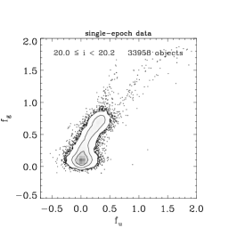
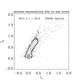
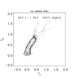
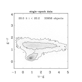
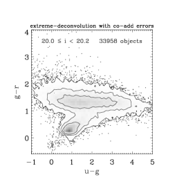
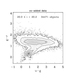
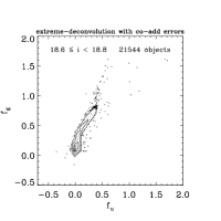
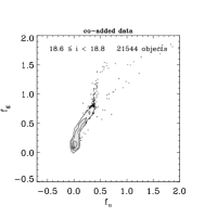
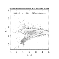
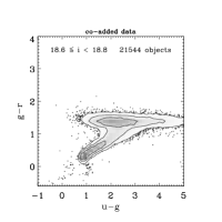
The XD method implicitly produces an error-deconvolved model of the relative-flux distribution, which would correspond to the true parent distribution of our training set in the limit of infinite signal-to-noise ratio. We refer to this as the ‘underlying’ model of the data. An important test of our approach is to apply the XD technique to the noisier single-epoch data of the stars in Stripe-82, and compare our determination of the underlying model to the much higher signal-to-noise ratio Stripe-82 co-added photometry of the same sources. This is a stringent test since the underlying model fit is based on much noisier single-epoch data than the co-added photometry.
If the co-added photometry were perfect, then the co-added data would represent samples of the underlying model with zero noise. In practice, even the Stripe-82 co-adds are noisy at the faint end, thus the relative-flux distribution of the co-adds will be correspondingly smoothed. To make a sensible comparison we sample the underlying model at the same number of points as are in the co-added catalog in a given magnitude bin, and convolve these samples with uncertainties of the co-added data. As we do not have a model for the noise in the co-added data, and our samples are in general at different locations in relative flux space, we simply match each sample from the underlying distribution to the closest object in the co-added catalog and use that co-add object’s uncertainties.
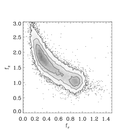
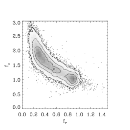
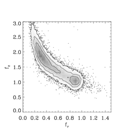
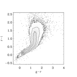
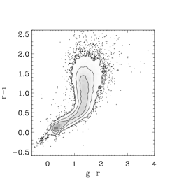
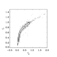
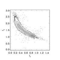
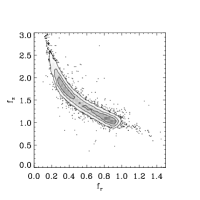
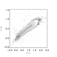
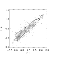
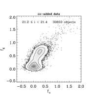
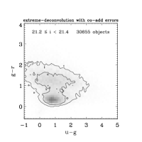
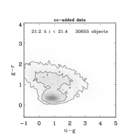
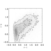
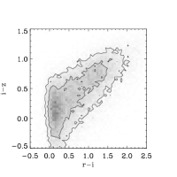
The results for this exercise for a single bin are shown in Figures 2 and 3. We see that the agreement between the model and the co-add truth is excellent.
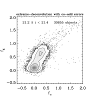
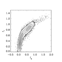
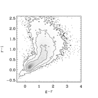
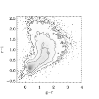
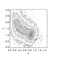
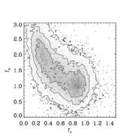
After fitting the relative flux distribution of the training data we can also compare the best-fit model with the training data by convolving the model with the data uncertainties. This uncertainty-convolution is again performed by matching a sampled point to the nearest object in the training set and drawing from that object’s uncertainty distribution. Some results of these tests are shown in Figures 4 to 6.
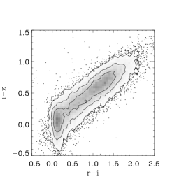
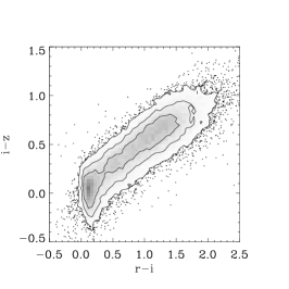
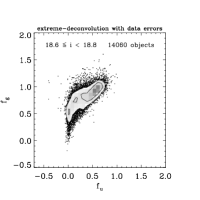
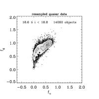
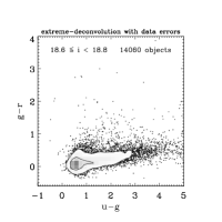
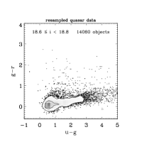
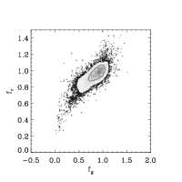
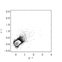
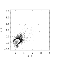
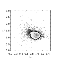
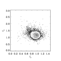
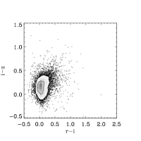
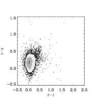
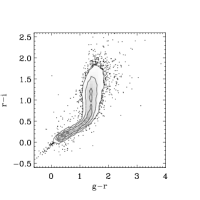
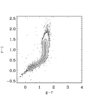
Figure 4 shows flux-flux and color-color diagrams in one of the bins in -band magnitude for medium-redshift quasars. The first and third columns show a sampling from the best-fit XD model to the relative fluxes. The second and fourth columns show the data that these fits were based on: These data are quasars from the SDSS DR7 quasar catalog resampled according to the quasar luminosity function as explained in Section 3.2. Similar figures for the other apparent magnitude bins are very similar as the distribution of quasar colors does not vary much with apparent magnitude. The same comparison for low- and high-redshift quasars was performed for quality assurance, but these figures are not shown here.
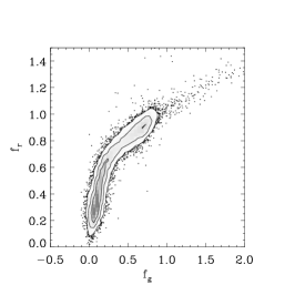
Figure 5 shows the comparison between the XD fit to the co-added point-source data from SDSS Stripe-82 and the data itself for a relatively bright apparent magnitude bin. Figure 6 shows the same for a fainter bin in -band apparent magnitude. In this bin the photometric uncertainties are significant such that the stellar locus is severely smoothed. We see that the underlying deconvolved XD model is good in the sense that after convolution with the data uncertainties it reproduces the observed distribution.
The resampled error-convolved fits to the data in all of these cases are essentially indistinguishable from the real data.
Section 5 The SDSS-XDQSO quasar targeting catalog
Using the models of quasar and stellar fluxes described in the previous Section we create a quasar targeting catalog. For every point source (objc_type = 6) in the SDSS Data Release 8 (DR8) with a reasonable detection333Defined to be those point sources for which the PSF magnitude in at least one of is brighter than (22.5, 22.5, 22.5, 22, 21.5) after correction for Galactic extinction following Schlegel et al. (1998) (Aihara et al., 2011). in at least one band that is primary and has a dereddened -band magnitude 17.75 we calculate the probability that the object is a quasar or star using equation (1). Specifically, we use the models from the previous Section as follows. For an object with dereddened -band magnitude we first find the bin for which this magnitude is contained within the central 0.1 mag of the bin (this is always possible since neighboring bins overlap by 0.1 mag). We use this bin to evaluate the relative-flux density for this object’s dereddened fluxes. We convolve the underlying 20 Gaussian mixture model with the object’s uncertainties as in equation (3). This uncertainty convolution is simply adding the object’s uncertainty variance to the intrinsic model variance for each component.
We further evaluate the number density as a function of apparent magnitude for the object’s -band flux. We do this for each of the classes (‘star’, and the three ‘quasar’ classes) and normalize the probabilities as in equation (2). Code that can be used to reproduce this information is made publicly available and is described in Appendix B.
For each object we also calculate the bitmask used for BOSS quasar target selection. This bitmask is calculated using version bosstarget v2_0_10 of the BOSS quasar target selection code. For the convenience of the user, we summarize this bitmask into a simple good flag. When this flag is zero the object passes all of the BOSS flag cuts; when the flag is one, the object fails one of the basic BOSS targeting flag criteria (interp_problems, deblend_problems, or moved). An object with a good flag equal to two fails one of the more esoteric BOSS quasar selection cuts. No objects with a good flag would be targeted by the BOSS. These flag cuts are discussed in more detail in Appendix A.
In addition to the quasar and star probabilities and flag-logic described above, we also report each of the factors in equation (4) for all of the target-classes for each object in the catalog. This allows the user of the catalog to substitute different number-count or relative-flux density models for any of the components.
A description of the catalog is given in Table 2. The full catalog contains 160,904,060 objects. Summing the probabilities, we expect this catalog to contain about 5,058,716 quasars, 2,551,146 of which are low-redshift, 1,410,405 are mid-redshift, and 1,097,165 are high-redshift. However, as we show below, this is probably a slight overestimate, especially for the high-redshift class.
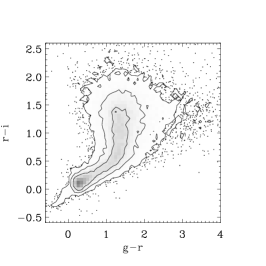
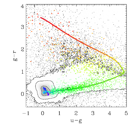
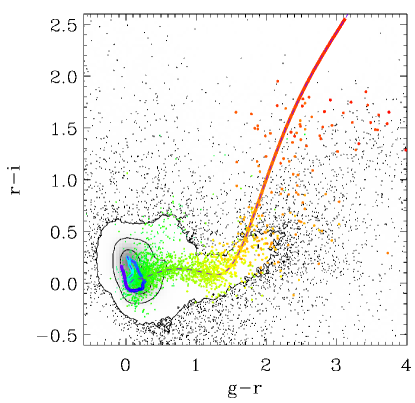
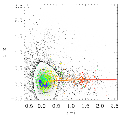
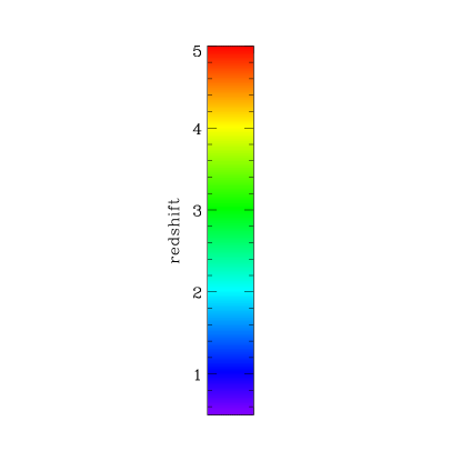
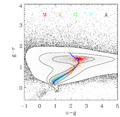
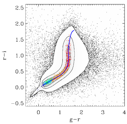
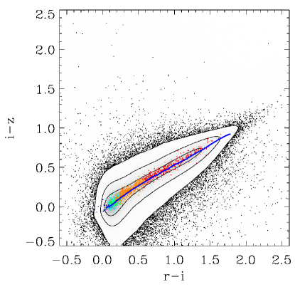
We stress that this quasar targeting catalog is entirely probabilistic and that the majority of objects are certainly stars. To create high-confidence quasar samples it is necessary to select those objects with the largest . As an example, we show in Figures 7 and 8 color–color plots of those objects in the SDSS-XDQSO catalog with and . For the photometric quasars in Figure 7 a sparse sampling of quasars from the SDSS DR7 quasar catalog (Schneider et al., 2010) and a model for the quasar locus from Hennawi et al. (2010) is shown for comparison. For the photometric stars in Figure 8 a model for the stellar locus from Hennawi et al. (2010) and some representative classes of stars along the stellar locus are shown. While we cannot be sure for any of the objects in either of these photometric samples whether they are truly quasars or stars, the color distribution of the ensemble does resemble that of a set of quasars and stars, respectively.
5.1 Catalog availability
The SDSS-XDQSO catalog is available through the SDSS-III DR8 Science Archive Server at
http://data.sdss3.org/sas/dr8/groups/boss/photoObj/xdqso/xdcore/ .
The catalog consists of a single fits file for each imaging run in the DR8 release (Aihara et al., 2011); filenames have the form xdcore_RUN6.fits, where RUN6 is the six-digit imaging run number. The catalog entries are described in Table 2, as well as in the SDSS-III datamodel at
http://data.sdss3.org/datamodel/files/BOSS_PHOTOOBJ/xdqso/xdcore/xdcore_RUN6.html
Section 6 Testing the catalog
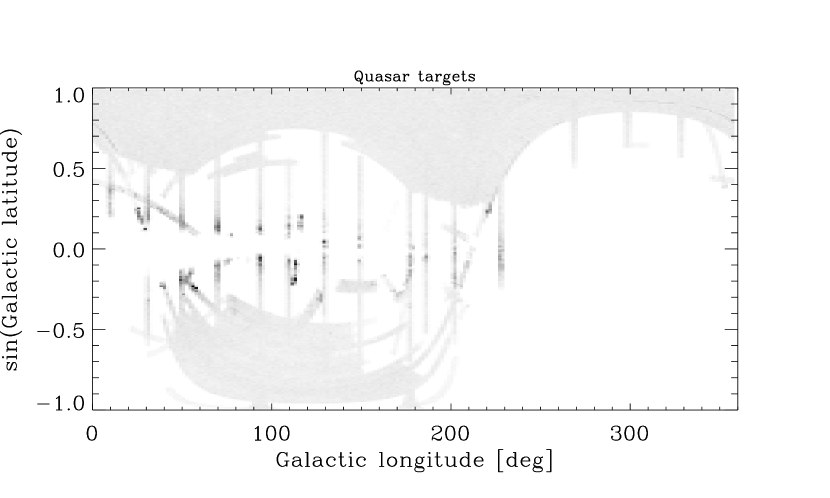
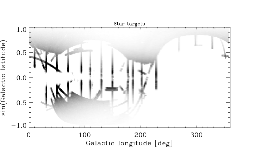
While there are many detailed considerations in constructing a specific quasar sample from the SDSS-XDQSO catalog, for the purposes of testing we use an arbitrarily chosen cut of to define a ‘quasar’ sample and to define a ‘star’ sample. We show the sky distribution of quasars and stars in Figure 9. As expected for a quasar catalog, the distribution is mostly flat, with only minor increases in density near the Galactic plane where the density of stars and hence potential contaminants is extremely high. This expected behavior is satisfying since our model did not include a prior depending on Galactic longitude and latitude. The stars selected by the star cut do show the expected strong dependence on Galactic latitude. If we had included a better prior depending on the Galactic latitude and longitude of targets, there would have been less quasar targets in regions closer to the Galactic plane, since objects would then get a higher probability of being stars. Quasar are targeted predominantly at high Galactic latitude, such that the inclusion of such a prior does not lead to great improvements to the targeting efficiency; therefore, we have not pursued this here.
In Figure 10 we show the XDQSO probabilities of known, i.e., spectroscopically confirmed, quasars and stars. These come from a compilation of known quasars and stars from various surveys, including some early BOSS data. We split the sample of known quasars into our three redshift bins. We see that both known low-redshift quasars and known stars are assigned very high probabilities for the correct class, with no significant populations of low-probability objects for a given class. The distribution of mid-redshift probabilities for known mid-redshift quasars shows that most of these quasars have high correct probabilities, but that there is a population of objects around . Inspection of the probabilities of being stars for these objects shows that not all of them get high star probabilities, such that at least some of these are ‘misclassified’ into the wrong redshift range. Most of the known high-redshift quasars are assigned high high-redshift probabilities, with only a small population being ‘misclassified’ as stars. The color-color distributions of ‘misclassified’ quasars show that many of these are quasars that overlap the stellar locus, such that it is unsurprising that color selection fails. The sky distribution of ‘misclassified’ quasars shows that many of these objects lie in SDSS Stripe-82, where deeper photometry for quasar selection is available than the single-epoch fluxes used in this comparison. These Stripe-82 quasars were probably targeted based on higher signal-to-noise co-added photometry, whereby they could be better distinguished from stars.
We have cross-correlated our catalog with the FIRST point-source catalog (Becker et al., 1995) with a matching radius of 0′′.5 (McGreer et al., 2009). We expect that most of these objects—optically unresolved point sources with compact radio morphology—are quasars, with only a small fraction being compact radio galaxies (McGreer et al., 2009). In Figure 11, we show the quasar probabilities for the matching FIRST objects. The majority of these sources have high quasar probabilities. Those that do not have high quasar probabilities either overlap with the stellar locus or have very unusual colors. An inspection of FIRST sources targeted as quasars by the BOSS shows that FIRST-selected quasars with small XDQSO quasar probabilities are significantly redder than quasars with high XDQSO probabilities; they are missed by the XDQSO method because it is trained on optically-selected quasars which are typically bluer than radio-selected quasars.
Finally, we show in Figure 12 the quasar probabilities for the uvx objects in the Richards et al. (2009a) photometric quasar catalog. We expect percent of these objects to be quasars. Only a small fraction of objects are assigned low quasar probabilities, which is unsurprising given the 95 percent efficiency of the photometric catalog. We discuss the Richards et al. (2009a) technique further in Section 8.1.1 in the specific context of target selection.
Section 7 BOSS quasar target selection
As discussed in the introduction, the BOSS aims to obtain spectra of quasars in the redshift range to observe the baryon acoustic feature in the Lyman- forest and obtain a percent-level measurement of the angular diameter distance to redshift 2.5. This requires observing at least 15 quasars deg-2 over the BOSS survey area. Since only about 40 targets deg-2 will be allocated for quasar targets, target selection must reach 50 percent efficiency to achieve this goal. Achieving this efficiency is complicated by the substantial overlap between the quasar and stellar loci in color-space in the BOSS redshift range and the need to target to mag where photometric uncertainties are significant.
While a uniform target selection of the BOSS quasars is unnecessary for the cosmological distance measurement because the quasars are only used to reveal the intervening Lyman- forest, the BOSS quasar target selection reserves 20 targets deg-2 for a “CORE” sample of objects that is selected by a single method over the course of the survey, to allow statistical studies of quasar properties. Since only single-epoch SDSS fluxes are available for the bulk of the BOSS survey footprint, this CORE sample must be based on these single-epoch fluxes alone.
The SDSS-XDQSO catalog presented in Section 5 allows such a uniform sample to be defined while maintaining a high target efficiency. In practice we use the medium-redshift quasar probabilities pqsomidz (see Table 2) and target all good objects with dereddened ( mag or mag) and mag—the BOSS flux limits—with pqsomidz larger than a threshold set to give 20 or 40 targets deg-2 over a certain region (e.g., a part of the survey such as Stripe-82 or the entire survey footprint).
Even though the XDQSO targeting technique was not used during the first year of BOSS data acquisition, we can nevertheless evaluate the XDQSO performance by determining how many of the XDQSO quasar targets are spectroscopically confirmed BOSS quasars. This is a conservative test as it presumes that the BOSS quasar sample is highly complete; any incompleteness would lead us to underestimate our efficiency since there would then be real quasars selected by XDQSO but which did not receive a BOSS fiber. In Figure 13 we show the XDQSO targeting efficiency in an area from the BOSS. This area consists of BOSS observations of Stripe-82. Since over eight epochs are available for most sources in Stripe-82, BOSS quasar target selection was based on deeper co-added data and included variability selection (Palanque-Delabrouille et al. 2011). Therefore, it is highly complete and it is therefore the best test of the XDQSO technique. We only use the deg2 region of Stripe-82 where at least 15 2.2 quasars deg-2 were observed by the BOSS; on average 27 quasars deg-2 are available. This is close to the total number of quasars in this redshift range expected based on various quasar luminosity functions (Richards et al., 2006; Jiang et al., 2006; Hopkins, Richards, & Hernquist, 2007). We see that at 20 targets deg-2 the efficiency is about 50 percent; the efficiency drops rapidly at higher target densities.
A further test of the XDQSO technique was performed during the Fall of 2010. Approximately 20 medium-redshift quasar targets (catalog tag pqsomidz) per square degree were observed as part of the BOSS in a region of deg2 just north of SDSS Stripe-82. As of 2010 November 22, 4,593 objects were targeted and 2,194 of these were classified as 2.2 quasars, corresponding to an efficiency of 48 percent. In Section 8.1 we compare the XDQSO selection to other targeting algorithms which were tested during the first year of BOSS commissioning.
We can also use the early BOSS data to evaluate whether the XDQSO probabilities given to objects are correct in the ensemble sense. That is, we can bin objects in and evaluate the fraction of these objects that are quasars. This test again assumes that the test sample of quasars is highly complete. The results from this exercise are shown in Figure 14. We see that the quasar probabilities appear to be overestimated. Several shortcomings of the model for the quasar and stellar populations could be responsible for this result. Since we used relatively small samples of stars in each bin compared to the number of quasars—the proportion being around one to one rather than reflecting the true number densities according to which stars outnumber quasars by a factor of down to mag—we probe much lower density regions for the quasars than we can for the stars. Thus, in low stellar-density regions, the stellar density is likely to be underestimated with respect to the quasar densities, leading to overestimated quasar probabilities in these regions. This is unlikely to change the ranking of quasar targets significantly—most targets will be affected in the same way. Thus, quasar targeting using the SDSS-XDQSO catalog is robust with respect to this modeling problem. However, this aspect of our analysis does merit caution when taking the specific value of the quasar probabilities serious in an analysis of quasar properties. Our model also does not include variations in the stellar number density with Galactic latitude and longitude, so the stellar density will be underestimated in regions closer to the Galactic plane. Several of the extensions described in Section 8.2 can be used to mitigate these problems with the catalog.
Section 8 Discussion
8.1 Comparison with other target selection methods
Several sophisticated methods already exist to select quasars from photometric SDSS data, especially for the mid-redshift range targeted in the BOSS.
8.1.1 Richards et al. (2009a) NBC-KDE
The NBC-KDE photometric quasar catalog of Richards et al. (2009a) also uses density estimation to calculate relative number densities of stars and quasars to determine quasar probabilities. It differs from the technique described in this paper in that it (a) uses colors rather than relative fluxes in equation (4), (b) assumes a flat probability distribution for , (c) uses a simple kernel density estimation technique of the observed distribution of colors, thus ignoring the flux uncertainties of the training data, and (d) ignores the flux uncertainties of the data at evaluation. Since the catalog is limited to mag, ignoring the flux uncertainties is mostly harmless, although medium and high redshift quasars have very low - and -band fluxes with large associated uncertainties. This assumption also makes it harder to extend the catalog to fainter magnitudes. The NBC-KDE catalog also does not compute exact kernel-density likelihoods for all of the SDSS data because of computational limitations. The XD technique permits these likelihoods to be computed for all of the data (see above).
We compare the XDQSO catalog with the NBC-KDE catalog by (a) limiting the XDQSO catalog to the SDSS DR6 footprint, since the NBC-KDE catalog only covers this area, (b) limiting the XDQSO catalog to mag, and (c) limiting the NBC-KDE catalog to , the bright limit of the XDQSO catalog. We select those targets in the NBC-KDE catalog with good and then select equal numbers of targets from the good entries in the XDQSO catalog in the three shared target classes of the two catalogs: lowz, midz, and highz. Note that the good flags in the two catalogs are different. The results of this comparison are given in Table 3. The confirmed quasars in this Table come from a compilation of all spectroscopically confirmed quasars. The bulk of these are SDSS quasars that were selected to be brighter than mag.
We stress that this comparison is significantly biased in favor of the NBC-KDE catalog: the NBC-catalog was allowed to set the target threshold and its good flag includes cuts on Galactic latitude that we did not apply to the XDQSO catalog. Nevertheless, we see that the two catalogs perform similarly for low-redshift quasars, and that the XDQSO technique performs better in the mid-redshift range where the quasar and stellar loci overlap and photometric target selection is difficult.
The NBC-KDE catalog performs better at high-redshift than the XDQSO catalog. This is not unexpected as we only used 150 deg2 of stellar data to train the XDQSO algorithm. The red-star stellar-locus outliers that contaminate quasar selection are very rare on the sky: If we assume that they are ten times more abundant than quasars we expect our stellar training set to only contain about 2,000 of these. This is not enough to model their color distribution since they are spread over all magnitude bins. In the following Section we discuss improvements to the XDQSO technique that can improve high-redshift quasar selection.
8.1.2 Yeche et al. 2009’s neural network
The quasar-selection technique of Yeche et al. (2009) uses a neural network (NN) to select quasars in the BOSS mid-redshift range. This technique uses as the input variables the four colors , , , and , the -band magnitude, and the five magnitude uncertainties. These 10 variables are propagated through a simple NN that is trained on sets of known quasars and point-like objects from SDSS DR7 to obtain an output parameter xnn on which potential targets can be ranked. A similar NN is used to find a photometric redshift znn for the quasar targets. To select targets in the mid-redshift range they recommend the cuts znn , , and . While this technique uses the photometric uncertainties, it does this in a black-box manner that is quite different from the probabilistic way in which XD treats the uncertainties; the NN approach cannot work well when the test set is noisier than the training set.
We use the version of the NN technique that is part of the official BOSS quasar selection framework to compare the XDQSO technique and the NN technique at different target densities using early BOSS data. For the NN we first make the cuts listed above and then rank the targets on xnn until we reach the desired target density. For XDQSO we rank the good targets based on pqsomidz (see Table 2). The results from this comparison for BOSS year-one observations of Stripe-82 are shown in Figure 13. We see that the neural network performs significantly worse than XDQSO at all target densities.
8.1.3 Kirkpatrick et al.’s Likelihood
The Likelihood technique of J. A. Kirkpatrick et al. (2011, in preparation) uses an approach similar to the NBC-KDE catalog. Rather than colors it uses fluxes, such that the apparent magnitude factor also used by XDQSO is automatically taken into account, and rather than a kernel with an optimized bandwidth, Likelihood uses a delta function—corresponding to a model of the underlying density consisting of delta functions centered at the location of each object in the respective training set. These delta functions are convolved with the flux-uncertainties at evaluation such that a smooth density is obtained nevertheless. The Likelihood technique uses a similar stellar training data as the XDQSO catalog. The quasar training set is also modeled by re-sampling the quasar luminosity function, but these are essentially the same set of quasars used to train the XDQSO technique. Rather than simulating relative fluxes only, a full quasar catalog with five-dimensional fluxes in the relevant magnitude range is simulated.
The Likelihood technique uses the flux uncertainties to smooth the discrete underlying delta-function distribution of its training sets. However, since it does not use an optimized bandwidth, there is the danger that the density might be undersmoothed in certain regions. At the faint end, where the training set has a significant contribution from the uncertainties, the Likelihood method also effectively convolves with the uncertainties twice. This follows because the training set is a sample from the observed distribution of fluxes, rather than the true underlying distribution; the former is the latter convolved with the uncertainty distribution. Finally, as with the NBC-KDE catalog, the calculation of the quasar and star probabilities is extremely slow compared to XDQSO. In our comparison below we use cached versions of the Likelihood catalog created by the BOSS target selection team.
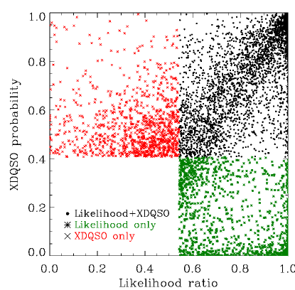
In Figure 15 we first compare the XDQSO quasar probabilities in the BOSS mid-redshift range with the probabilities calculated using the Likelihood method for sources in Stripe-82. We select targets at 20 targets deg-2 and show those targets selected by both techniques or by only one of the techniques. While many of the targets cluster around the one-to-one line, there is a distinct population of targets that receive high Likelihood probabilities, yet low XDQSO probabilities. A similar population of high XDQSO-only targets is absent, indicating that the Likelihood method indeed has problems with undersmoothing.
In Figure 13 we compare the XDQSO catalog with the Likelihood technique at different target densities. The two methods perform similarly, with a slightly better performance for the XDQSO catalog over the whole range.
A further comparison between the XDQSO and the Likelihood methods for medium-redshift quasar selection was performed during the Fall of 2010 using BOSS observations of an deg2 region just north of Stripe-82 (see Section 7). Both methods were given similar target densities to allow for a direct comparison. As of 2010 November 22, XDQSO was given 4,593 targets, while Likelihood received 4,853 targets. Of the 4,593 XDQSO targets 2,194 were classified as 2.2 quasars, while of the 4,853 Likelihood targets only 2,056 turned out to be medium-redshift quasars. From this test and that in Figure 13 we conclude that the XDQSO technique’s performance is about 10 percent better than that of the Likelihood method for the selection of medium-redshift quasars.
8.2 Extensions
One of the main advantages of the general target selection technique and in particular of the specific XDQSO implementation described in this Article is that it can easily be extended in a variety of ways. These extensions can be changes to the model—such as different number count priors, the addition to the model of other data such as NIR or UV observations—or the combination of the flux-based selection described here with target selection based on variability information. All of these extensions are described briefly here.
Most of these extensions involve only some of the factors in equations (1) and (4). Since we provide all of these factors separately in the SDSS-XDQSO catalog, extensions that do not change all of the factors can use some of the information in the catalog. For example, extensions that only change the number count priors, e.g., or , will not need to re-calculate the relative-flux likelihoods—the most expensive of the factors in equation (4)–but can instead re-use the catalog values.
8.2.1 Additional NIR or UV data
Quasar selection from broad-band fluxes can be improved by the addition of NIR or UV fluxes to the optical fluxes used to create the SDSS-XDQSO catalog (e.g., Warren et al., 2000; Maddox et al., 2008; Richards et al., 2009b; Jimenez et al., 2009; Worseck & Prochaska, 2010). For example, the Galaxy Evolution Explorer (GALEX; Martin et al. 2005) has completed a near full-sky survey in the ultraviolet (UV) and the UKIRT Infrared Deep Sky Survey (UKIDSS; Lawrence et al. 2007) is observing a large part of the SDSS footprint in the NIR. However, this situation is complicated by the fact that these surveys are generally shallower than the optical fluxes available from SDSS, such that most of the objects in the SDSS catalog are not detected at high significance in these surveys.
Since these surveys have point-spread functions that are worse than that of the SDSS, low signal-to-noise measurements of the NIR and UV fluxes of many of the objects in the SDSS catalog can be obtained by forced photometry of the GALEX or UKIDSS images at the SDSS positions, which can be regarded as truth because of the difference in resolution. Because there are gaps in these surveys, it will still be the case that some objects in both the training set and the evaluation set will not have measured NIR or UV fluxes.
To use these low signal-to-noise or non-existent fluxes, it is necessary to employ a classifier than can handle the data uncertainties correctly and that can handle missing data, both for training and for evaluation of the quasar probabilities. The XDQSO method described in this Article is the only technique to date that can do this task naturally and it is therefore the only method available that—in a straightforward way—can use all of the available information for an object to classify it as a star or quasar.
The procedure to use the NIR or UV data is the following: We combine the optical fluxes in our training sets of quasars and stars with the available NIR or UV data. We then train the XD model for the relative fluxes on the combined relative optical plus NIR or UV fluxes, using missing relative fluxes—e.g., by using a very large uncertainty variance for these—where NIR or UV fluxes do not exist. Then for those objects in the evaluation set (e.g., the SDSS DR8 catalog) with measured NIR or UV fluxes, we replace the relative-flux likelihoods based on fluxes in the SDSS-XDQSO catalog with those likelihoods calculated using optical plus NIR or UV fluxes. The apparent -band magnitude factors do not change, as these are functions of alone.
This selection can then be used to select targets based on combined GALEX and SDSS data, or to use GALEX fluxes instead of the highly discriminating -band fluxes for surveys such as Pan-STARRS that do not have a band (Jimenez et al. 2009; J. Bovy et al., 2011, in preparation). It can also be used to select targets based on SDSS and UKIDSS fluxes where the SDSS and UKIDSS overlap, or to use only some of the redder optical bands plus NIR data to avoid potential biases due to the inclusion of bluer optical bands (Worseck & Prochaska, 2010).
8.2.2 Variability
With the opening of the time-domain in the near-future with surveys such as Pan-STARRS (Kaiser et al., 2002; Morgan et al., 2008), LSST (Ivezić et al., 2008; Abell et al., 2009), Skymapper (Keller et al., 2007), and WFIRST, the selection of quasars based on their variability has recently received some attention (Kozłowski et al., 2010; Schmidt et al., 2010; Butler & Bloom, 2010; MacLeod et al., 2010). Some of these techniques currently amount to drawing the equivalent of “color-boxes” in variability space to select quasars (Schmidt et al., 2010; MacLeod et al., 2010), while others perform more sophisticated model selection (Butler & Bloom, 2010). However, it is clear that the variability technique could be brought under the umbrella of probabilistic target selection by doing density estimation in the space of variability attributes (such as parameters of the structure function) in a similar manner as we did in flux space in this Article.
The variability data can be used to form a variability-likelihood similar to the relative-flux likelihood used in equation (4). If we assume that the variability of a quasar is independent of its (relative) flux—not necessarily a good assumption—we can combine the relative-flux and variability likelihoods by simply multiplying the quantities. Alternatively, we can perform density estimation in the combined space of relative fluxes and variability parameters, and use the combined likelihood instead of the relative-flux likelihood in equation (4)—this will capture any (relative) flux dependence of the variability of quasars. Combining variability and flux information is our best hope to create extremely efficient quasars surveys in the future that are free from the biases associated with color or variability selection alone.
8.2.3 Other extensions
All of the factors in equation (4) can be improved upon using existing data and the XDQSO target selection technique. For example, we used a star count model that is not a function of Galactic coordinates, but we know that the number density of stars is a strong function of Galactic latitude and Galactic longitude. Both the total stellar number counts in Table 1 and the stellar number counts as a function of apparent magnitude in Figure 1 could be re-calculated using models for the stars counts in different directions. However, this will not lead to significant changes in the calculated quasar and star probabilities, as the distribution on the celestial sphere of photometrically selected quasars and stars already follows the expected celestial distributions of quasars and stars quite well (see above and Figure 9).
We also used relative-flux distributions for the stars that do not depend on the celestial location of an object. However, the colors of stars do change with proximity to the plane of the Galaxy. Therefore, we could have used a model that reconstructs the relative flux distribution of stars as a function of the position on the sky. Such a model is hard to produce from the current data, if we do not want to rely on theoretical models for this dependence, since we have no way a priori to separate quasars from stars all over the sky. What we can do is model the relative-flux distribution of all point sources as a function of position on the sky, from the single-epoch SDSS fluxes available on the SDSS footprint. In order to use the noisy single-epoch fluxes properly, it is again necessary to use a technique such as XDQSO that uses the uncertainties correctly. Using the model for the quasar fluxes that we have been using in this Article we can calculate quasar probabilities by using the quasar model in the numerator of equation (2) and the model for all point sources in the denominator. However, it is then possible for the probability to exceed one, since the probability is not explicitly normalized.
We could also use a training set consisting of point sources over the entire SDSS footprint rather than the 150 deg2 area of Stripe-82 to increase our sampling of rare stellar-locus outliers. As mentioned above, red stellar-locus outliers outnumber high-redshift quasars and are a significant contaminant for high-redshift quasar selection. Our current training set does not contain enough of these red stellar outliers to model their relative flux distribution. By extending our stellar training sample to the full deg2 SDSS footprint we would have about 100 times more stellar outliers and we could model their color distribution. This would significantly improve high-redshift quasar target selection.
8.3 Decision theory
Inference (Bayesian or frequentist) only assigns relative probabilities on outcomes or models. It does not tell you what to do; this also involves your capability, e.g., the number of fibers you can use per square degree and their minimal spacing, and your utility, e.g., signal-to-noise in the Lyman- forest for the BOSS quasar baryon-acoustic-feature detection. The decision to cut metal in the spectroscopic plate (in the case of the BOSS) is a hard decision that cannot, in the end, be probabilistic. The probabilistic results permit calculations of expected utility, which can be used to set decisions, such as whether to prefer quasar targets to luminous-red-galaxy targets in the case of fiber collisions in the BOSS. The BOSS targeting decisions are unlikely to be made this way, but in situations in which inference is accurate, and (this is rarer) utility can be calculated, it should improve overall efficiency and capability.
To be more specific, different quasars with different properties will have different value for any individual scientific project. For example, for the Lyman- baryon acoustic feature analysis the BOSS is expected to obtain more information from quasars that are brighter, and quasars in certain redshift ranges. At the same time, different quasars with different properties will be easier and harder to select, because of their photometric differences and similarities with stellar sources or other contaminants. It will usually be a frequent occurrence that one will decide, when comparing two sources, to target the object less likely to be a quasar because the lower probability is compensated by greater value to the survey if the object is indeed a quasar.
Additionally, some classes of contaminants can have higher utility than others, and one might decide to preferentially target quasars that are more likely to be confused with useful contaminants. For example, some contaminants for the BOSS quasar target selection are BHB stars, which are very useful for studies of Galactic structure (e.g., Xue et al., 2008), and hypervelocity stars. Future surveys might decide to combine different science goals with different classes of targets, and probability-based utilities are then essential to most efficiently achieve all of the science goals.
Section 9 Conclusion
The XDQSO method described in this Article is a new general target selection technique that can be used to design highly efficient surveys for faint objects that are hard to distinguish from contaminants based on their measured attributes. This high efficiency is achieved through the use of the extreme-deconvolution density-estimation to classify objects based on the number densities of desired objects and contaminants in attribute space. We used this approach to create an input catalog for BOSS quasar target selection, which aims to target quasars over deg2 at 50-percent efficiency down to mag. Quasar colors in this redshift range overlap strongly with stellar colors and classification is made even more difficult by the large photometric uncertainties at these faint magnitudes. We demonstrated that at the 20 targets deg-2 required for the BOSS ‘CORE’ sample the XDQSO technique is indeed approximately 50 percent efficient and that it outperforms all other medium-redshift quasar target selection techniques.
We release the full 160,904,060-object SDSS-XDQSO quasar targeting catalog containing star and low-, medium- and high-redshift quasar probabilities for all primary objects in the dereddened -band magnitude range in SDSS DR8. We also release code to reproduce the catalog from the SDSS point-source catalog.
The XDQSO target selection technique can be extended to include low signal-to-noise data in NIR and UV filters and to include other information such as quasar variability. It is the low signal-to-noise ratio regime at the faint edge of surveys that often contains the most interesting objects. XDQSO is the only target selection technique currently available that can calculate robust quasar probabilities taking the data-uncertainties fully into account. Since the most successful photometric quasar catalogs are based on calculating good photometric quasar probabilities (Richards et al., 2009a), the XDQSO technique or similar will be essential to create the best and largest photometric quasar catalogs in upcoming surveys such as Pan-STARRS and LSST.
Appendix A Flag Cuts
As part of the information in our catalog, we include an entry good that facilitates two different sets of useful flag cuts. One set is the BOSS flag cuts, which are appropriate when attempting to use the information in the catalog directly for statistical studies. For objects that do not pass this set of flag cuts, good . The second set of flag cuts is less restrictive, and is more appropriate for follow-up observations where high completeness is required (such as, for instance, a search for high redshift quasars). For objects that do not pass this less restrictive set of flag cuts, good = 1. Objects that pass these cuts but fail other BOSS flag cuts have good = 2.
We also provide a flag photometric, which is not bitwise—it is either True or False—and can be utilized at the user’s discretion. This is a standard SDSS flag: photometric refers to objects that were observed under good imaging conditions. Restricting to photometric affects the coverage of the catalog and should only be considered when constructing a highly restrictive sample.
A.1 good = 1
Our less restrictive set of flag cuts (good = 1) slightly
differs from the standard BOSS quasar targeting flags. They use
broader magnitude limits of (extincted PSF
luptitudes) and only adopt a subset of the raw flag cuts. We adopt the
raw flag cut definitions detailed in Stoughton et al. (2002), except
for gerr, rerr and ierr, which denote errors on extincted PSF
luptitudes in the , and bands, and for the column and row
movement information. First, two sets of flag cuts are defined from
the raw flag cuts, denoting whether the photometric pipeline had
difficulty deblending or interpolating a source:
interp_problems = (psf_flux_interp && ()) bad_counts_error (interp_center && cr)
deblend_problems = peakcenter notchecked (deblend_nopeak && ())
where symbols (&&, , !) denote standard Boolean logic. moved is set if the raw flag deblended_as_moving is set and if the value and error on the row or column position in the SDSS imaging pipeline (rowv, colv, rowverr, colverr) suggest a move across a row or a column. Then, if (interp_problems deblend_problems moved) we set good = 1.
A.2 good =
The flag cuts leading to good = 1 are less restrictive than the BOSS quasar survey flags. Additional flag cuts to mimic the BOSS flags use magnitude limits of where magnitudes are extincted PSF luptitudes. Then for objects passing the good = 1 flag cuts we have:
IF ((!binned1 bright saturated edge blended nodeblend noprofile) && !(interp_problems deblend_problems moved)) THEN (good = 2)
All of our individual flag cuts are also recorded as a mask of bits (called bitmask). For most users, we recommend a cut at good != 1 for follow-up observations and good = 0 for direct statistical analyses or to mimic BOSS targeting. For users brave enough to use our catalog beyond this level of sophistication, bitmask can be used to back out individual flag cuts. bitmask conforms to the values listed in the BOSS Target Selection Framework paper (E. S. Sheldon et al., 2011, in preparation).
Appendix B Target selection code
The XDQSO target-selection technique described in Section 4 is made publicly available at
http://data.sdss3.org/sas/dr8/groups/boss/photoObj/xdqso/xdqso-code.tar.gz
as a set of data files containing the parameters of the model and code that calculates the XDQSO likelihoods and probabilities. The data files need to be saved in a directory given by an environment variable $XDQSODATA. The data files consist of text files containing the number count priors of Table 1 and Figure 1 and FITS files containing the XD models for all of the bins with one file for each target class. Each FITS file contains 47 extensions, where extension contains a structure with the amplitudes (tag xamp), means (tag xmean), and covariance matrices (tag xcovar) for bin in -band magnitude.
In the IDL implementation the procedure xdqso_calculate_prob takes as input a structure containing tags psfflux, psfflux_ivar, and, if the option /dereddened is not set, extinction containing the fluxes, inverse flux-variances, and extinction values in the five SDSS bands. This is the structure of the SDSS ‘sweeps’ calibobj444See http://data.sdss3.org/datamodel/files/PHOTO_SWEEP/RERUN/calibObj.html . files. The output is a structure that mirrors the input structure and contains all of the XDQSO likelihoods, number count priors, and probabilities as given in the catalog description in Table 2. It is more efficient to run the code on arrays of objects rather than on objects individually, as each data file is read only once.
References
- Abazajian et al. (2003) Abazajian, K. N., et al., 2003, AJ, 126, 2081
- Abazajian et al. (2009) Abazajian, K. N., et al., 2009, ApJS, 182, 543
- Abell et al. (2009) Abell, P. A., et al., 2009, The LSST Science Book, arXiv:0912.0201v1 [astro-ph]
- Adelman-McCarthy et al. (2006) Adelman-McCarthy, J. K., et al., 2006, ApJS, 162, 38
- Adelman-McCarthy et al. (2008) Adelman-McCarthy, J. K., et al., 2008, ApJS, 175, 297
- Aihara et al. (2011) Aihara, H., et al., 2011, ApJS, submitted, arXiv:1101:1559
- Arp (1970) Arp, H., 1970, AJ, 75, 1
- Baldwin (1977) Baldwin, J. A., 1977, ApJ, 214, 679
- Becker et al. (1995) Becker, R. H., White, R. L., & Helfand, D. J., 1995, ApJ, 450, 559
- Bishop (1995) Bishop, C. M., 1995, Neural Networks for Pattern Recognition (Oxford University Press)
- Bovy et al. (2009) Bovy, J., Hogg, D. W., & Roweis, S. T. 2009, AOAS, in press, arXiv:0905.2979v1 [stat.ME]
- Butler & Bloom (2010) Butler, N. R. & Bloom, J. S., 2010, AJ, submitted, arXiv:1008.3143v1 [astro-ph]
- Chelouche et al. (2007) Chelouche, D., Koester, B. P., & Bowen, D. V., 2007, ApJ, 671, L97
- Dempster et al. (1977) Dempster, A. P., Laird, N. M., & Rubin, D. B., 1977, J. R. Stat. Soc. B, 39, 1
- Eisenstein et al. (2011) Eisenstein, D. J, et al., 2011, AJ, submitted, arXiv:1101:1529
- Fan (1999) Fan, X., 1999, AJ, 117, 2528
- Fukugita et al. (1996) Fukugita, M., Ichikawa, T., Gunn, J. E., Doi, M., Shimasaku, K., & Schneider, D. P., 1996, AJ, 111, 1748
- Giannantonio et al. (2008) Giannantonio, T., Scranton, R., Crittenden, R. G., Nichol, R. C., Boughn, S. P., Myers, A. D., & Richards, G. T., 2008, Phys. Rev. D, 77, 123520
- Giannantonio et al. (2006) Giannantonio, T., et al., 2006, Phys. Rev. D, 74, 063520
- Gunn et al. (1998) Gunn, J. E., et al., 1998, AJ, 116, 3040
- Gunn et al. (2006) Gunn, J. E., et al., 2006, AJ, 131, 2332
- Hawkins & Reddish (1975) Hawkins, M. R. S. & Reddish, V. C., 1975, Nature, 257, 772
- Hennawi et al. (2006) Hennawi, J. F., et al., 2006, AJ, 131, 1
- Hennawi et al. (2010) Hennawi, J. F. , et al., 2010, ApJ, 719, 1672
- Hogg et al. (2001) Hogg, D. W., Finkbeiner, D. P., Schlegel, D. J., & Gunn, J. E., 2001, AJ, 122, 2129
- Hopkins, Richards, & Hernquist (2007) Hopkins, P. F., Richards, G. T., & Hernquist, L., 2007, ApJ, 654, 731
- Ivezić et al. (2003) Ivezić, Ž., et al., 2003, Mem. Soc. Astron. Italiana, 74, 978
- Ivezić et al. (2004) Ivezić, Ž., et al., 2004, AN, 325, 583
- Ivezić et al. (2007) Ivezić, Ž., et al., 2007, AJ, 134, 973
- Ivezić et al. (2008) Ivezić, Ž., et al., 2008, arXiv:0805.2366v1 [astro-ph]
- Jiang et al. (2006) Jiang, L., et al., 2006, AJ, 131, 2788
- Jimenez et al. (2009) Jimenez, R., Spergel, D. N., Niemack, M. D., Menanteau, F., Hughes, J. P., Verde, L., & Kosowsky, A., 2009, ApJS, 181, 439
- Kaiser et al. (2002) Kaiser, N., et al., 2002, Proc. SPIE, 4836, 154
- Keller et al. (2007) Keller, S. C., et al., 2007, PASA, 24, 1
- Kozłowski et al. (2010) Kozłowski, S., et al., 2010, ApJ, 708, 927
- Lawrence et al. (2007) Lawrence, A., et al., 2007, MNRAS, 379, 1599
- Lupton et al. (2001) Lupton, R., et al., 2001, ASPC, 238, 269
- MacLeod et al. (2010) MacLeod, C. L., et al., 2011, ApJ, 728, 26
- Maddox et al. (2008) Maddox, N., Hewett, P. C., Warren, S. J., & Croom, S. M., 2008, MNRAS, 386, 1605
- Marshall et al. (1984) Marshall, H., et al., 1984, ApJ, 283, 50
- Martin et al. (2005) Martin, D. C., et al., 2005, ApJ, 619, L1
- McDonald & Eisenstein (2007) McDonald, P. & Eisenstein, D. J., 2007, Phys. Rev. D, 76, 063009
- McGreer et al. (2009) McGreer, I. D., Helfand, D. J., & White, R. L., 2009, AJ, 138, 1925
- Ménard et al. (2010) Ménard, B., Scranton, R., Fukugita, M., & Richards, G., 2010, MNRAS, 405, 1025
- Morgan et al. (2008) Morgan, J. S., et al., 2008, Proc. SPIE, 7012, 70122R
- Myers et al. (2006) Myers, A. D., Brunner, R. J., Richards, G. T., Nichol, R. C., Schneider, D. P., Vanden Berk, D. E., Scranton, R., Gray, A. G., & Brinkmann, Jon, 2006, ApJ, 638, 622
- Myers et al. (2007a) Myers, A. D., Brunner, R. J., Nichol, R. C., Richards, G. T., Schneider, D. P. & Bahcall, N. A., 2007a, ApJ, 658, 85
- Myers et al. (2007b) Myers, A. D., Brunner, R. J., Nichol, R. C., Richards, G. T., Schneider, D. P. & Bahcall, N. A., 2007b, ApJ, 658, 99
- Myers et al. (2008) Myers, A. D., Richards, G. T., Brunner, R. J., Schneider, D. P., Strand, N. E., Hall, P. B., Blomquist, J. A., & York, D. G., 2008, ApJ, 678, 635
- Oke & Gunn (1983) Oke, J. B. & Gunn, J. E., 1983, ApJ, 266, 713
- Osmer (1981) Osmer, P. S., 1981, ApJ, 247, 762
- Padmanabhan et al. (2008) Padmanabhan, N., et al., 2008, ApJ, 674, 1217
- Palanque-Delabrouille et al. (2011) Palanque-Delabrouille, et al., 2010, A&A, submitted, arXiv:1012.2391
- Pier et al. (2003) Pier, J. R., et al., 2003, AJ, 125, 1559
- Rasmussen & Williams (2006) Rasmussen, C. E. & Williams, C., 2006, Gaussian Processes for Machine Learning (MIT Press)
- Richards et al. (2002) Richards, G. T., et al., 2002, AJ, 123, 2945
- Richards et al. (2004) Richards, G. T., et al., 2004, ApJS, 155, 257
- Richards et al. (2006) Richards, G. T., et al., 2006, AJ, 131, 2766
- Richards et al. (2009a) Richards, G. T., et al., 2009a, ApJS, 180, 67
- Richards et al. (2009b) Richards, G. T., et al., 2009b, AJ, 137, 3884
- Ross et al. (2009) Ross, N. P., et al., 2009, ApJ, 697, 1634
- Sandage & Wyndham (1965) Sandage, A. & Wyndham, J. D., 1965, ApJ, 141, 328
- Schlegel et al. (2007) Schlegel, D. J., et al., 2007, in Bulletin of the American Astronomical Society, Vol. 38, 966
- Schlegel et al. (1998) Schlegel, D. J., Finkbeiner, D. P., & Davis, M., 1998, ApJ, 500, 525
- Schmidt et al. (2010) Schmidt, K. B., et al., 2010, ApJ, 714, 1194
- Schmidt & Green (1983) Schmidt, M. & Green, R. F., 1983, ApJ, 269, 352
- Schneider et al. (2010) Schneider, D. P., et al., 2010, AJ, 139, 2360
- Schölkopf & Smola (2002) Schölkopf, B. & Smola, A. J., 2002, Learning with Kernels: Support Vector Machines, Regularization, Optimization, and Beyond (MIT Press)
- Scranton et al. (2005a) Scranton, R., et al., 2005a, ApJ, 633, 589
- Scranton et al. (2005b) Scranton, R., et al., 2005b, arXiv:astro-ph/0508564
- Shen et al. (2007) Shen, Y., et al., 2007, AJ, 133, 2222
- Shen et al. (2010) Shen, Y., et al., 2010, ApJ, 719, 1693
- Smith et al. (2002) Smith, J. A., et al., 2002, AJ, 123, 2121
- Stoughton et al. (2002) Stoughton, C., et al., 2002, AJ, 123, 485
- Warren et al. (2000) Warren, S. J., Hewett, P. C., & Foltz, C. B., 2000, MNRAS, 312, 827
- Worseck & Prochaska (2010) Worseck, G. & Prochaska, J. X., 2011, ApJ, 728, 23
- Xue et al. (2008) Xue, X. X., et al., 2008, ApJ, 684, 1143
- Yeche et al. (2009) Yeche, C., et al., 2009, A&A, 523, A14
- Yip et al. (2004) Yip, C. W., et al., 2004, AJ, 128, 2603
- York et al. (2000) York, D. G., et al., 2000, AJ, 120, 1579
| Star | ||||||||
|---|---|---|---|---|---|---|---|---|
| Quasar | Quasar | Quasar | ||||||
| Number counts (deg-2) | 140. | 72 | 50. | 70 | 6. | 13 | 5209. | 38 |
| Column | Description |
|---|---|
| objId | Unique SDSS identifier\ref{objid}\ref{objid}footnotemark: |
| run | SDSS imaging run number |
| rerun | SDSS processing rerun number |
| camcol | Camera column |
| field | Field number |
| id | The object id within a field |
| RA | Right ascension in decimal degrees (J2000.0) |
| Dec | Declination in decimal degrees (J2000.0) |
| photometric | Indicates whether this object was observed under good imaging conditions (True/False) |
| psfMag | PSF übercalibrated asinh magnitude (corrected for Galactic extinction) |
| psfMagErr | Error in PSF asinh magnitude |
| extinction_u | Extinction in band; |
| qsolowzlike | Relative-flux density factor |
| qsomidzlike | Same as previous, but for the quasar class |
| qsohizlike | Same as previous, but for the quasar class |
| starlike | Same as previous, but for the ‘star’ class |
| qsolowznumber | Number density as a function of apparent magnitude for this object for the |
| quasar class (in deg-2 mag-1; =) | |
| qsomidznumber | Same as previous, but for the quasar class |
| qsohiznumber | Same as previous, but for the quasar class |
| starnumber | Same as previous, but for the ‘star’ class |
| pqsolowz | Probability that the object is a quasar |
| pqsomidz | Probability that the object is a quasar |
| pqsohiz | Probability that the object is a quasar |
| pqso | Probability that the object is a quasar (sum of previous three) |
| pstar | Probability that the object is a star |
| bitmask | BOSS quasar target selection bitmask |
| good | good flag: 0: passes all BOSS cuts, 1: fails basic BOSS cut (see text), |
| 2: fails other BOSS cuts (see Appendix A) |
| confirmed | confirmed | confirmed | |
|---|---|---|---|
| quasar | quasar | quasar | |
| NBC-KDE | 77144 | 11485 | 2802 |
| XDQSO | 77517 | 12711 | 2338 |
| total # targets | 569785 | 151860 | 9086 |

