SDSS Data Management and Photometric Quality Assessment

Abstract

We summarize the Sloan Digital Sky Survey data acquisition and processing steps, and describe runQA, a pipeline designed for automated data quality assessment. In particular, we show how the position of the stellar locus in color-color diagrams can be used to estimate the accuracy of photometric zeropoint calibration to better than 0.01 mag in 0.03 deg² patches. Using this method, we estimate that typical photometric zeropoint calibration errors for SDSS imaging data are not larger than $\sim 0.01$ mag in the $g$, $r$, and $i$ bands, 0.02 mag in the $z$ band, and 0.03 mag in the $u$ band (root-mean-scatter for zeropoint offsets).

1 Introduction

Modern large-scale digital sky surveys, such as SDSS, 2MASS, and FIRST, are opening new frontiers in astronomy. Due to large data rates, they require sophisticated data acquisition, processing and distribution systems. The quality of data is of paramount importance for their scientific impact, but its quantitative assessment is a difficult problem – mainly because it is not known very precisely what measurement values to expect. In the majority of large surveys to date, data quality assessment has not been fully automated and has required substantial human intervention – a significant shortcoming and resource sink when the data rate and volume are large.

The SDSS (Sloan Digital Sky Survey, York et al. 2000, Abazajian et al. 2003) is an optical imaging and spectroscopic survey, which aims to cover one quarter of the sky, and obtain high-quality spectra for 100,000 quasars, a similar number of stars, and a million galaxies. The SDSS observing, data processing, and data dissemination are highly automated operations – occasionally, SDSS is referred to as a science factory (to date, over a thousand journal papers are based on, or refer to, SDSS). We provide a brief summary of these operations in Section 2.

As has been the case for other surveys with large data rates, the data quality assessment and assurance has been a hard problem for SDSS. Recently, we have developed a set of tools, organized in the runQA pipeline, that are used to automatically assess the quality of SDSS imaging data products, and report all instances where it is substandard. The main ideas and results are described in Section 3, and further discussed in Section 4.

2 SDSS data flow and processing

2.1 Overview of SDSS imaging data

SDSS is providing homogeneous and deep ($r<22.5$) photometry in five pass-bands ($u$, $g$, $r$, $i$, and $z$, Fukugita et al. 1996; Gunn et al. 1998; Smith et al. 2002; Hogg et al. 2002) accurate to 0.02 mag (rms, for sources not limited by photon statistics, Ivezić et al. 2003). The survey sky coverage of 10,000 deg² in the Northern Galactic Cap, and $\sim 200$ deg² in the Southern Galactic Hemisphere, will result in photometric measurements for over 100 million stars and a similar number of galaxies. Astrometric positions are accurate to better than 0.1 arcsec per coordinate (rms) for sources with $r<20.5^{m}$ (Pier et al. 2003), and the morphological information from the images allows reliable star-galaxy separation to $r\sim$ 21.5^m (Lupton et al. 2002).

2.2 Data acquisition

The data acquisition system (Petravick et al. 1994) records information from the imaging camera, spectrographs, and photometric telescope (used to obtain photometric calibration data). The imaging camera produces the highest data rate ($\sim$ 20 GB/hour). Each system uses report files to track the observations.

Data from the imaging camera (thirty photometric, twelve astrometric, and two focus CCDs, Gunn et al. 1998) are collected in the drift scan mode. The images that correspond to the same sky location in each of the five photometric filters (these five images are collected over $\sim$5 minutes, with 54 sec per individual exposure) are grouped together for processing as a field. Frames from the astrometric and focus CCDs are not saved, but rather, stars from them are detected and measured in real time to provide feedback on telescope tracking and focus. This same analysis is done for the photometric CCDs, and we save these results along with the actual frames.

Data from the spectrographs are read from the four CCDs (one red channel and one blue channel in each of the two spectrographs) after each exposure. A complete set of exposures includes bias, flat, arc, and science exposures taken through the fibers, as well as a uniformly illuminated flat to take out pixel-to-pixel variations.

Data from the photometric telescope (PT) include bias frames, dome and twilight flats for each filter, measurements of primary standards in each filter, and measurements of secondary calibration patches (calibrated using primary standards, and sufficiently faint to be unsaturated in the main survey data) in each filter.

All of these systems are supported by a common set of observers’ programs, with observer interfaces customized for each system to optimize the observing efficiency.

2.3 Data processing factory

Data from Apache Point Observatory (APO) are transferred to Fermilab for processing and calibration via magnetic tape (using a commercial carrier), with critical, low-volume samples sent over the Internet. Imaging data are processed with the imaging pipelines: the astrometric pipeline (astrom) performs the astrometric calibration (Pier et al. 2003); the postage-stamp pipeline (psp) characterizes the behavior of the point-spread function (PSF) as a function of time and location in the focal plane; the frames pipeline (frames) finds, deblends, and measures the properties of objects; and the final calibration pipeline (nfcalib) applies the photometric calibration to the objects. This calibration uses the results of the PT data processed with the monitor telescope pipeline (mtpipe). The combination of the psp and frames pipelines is sometimes referred to as photo (Lupton et al. 2002).

Individual imaging runs that interleave are prepared for spectroscopy with the following steps: resolve selects a primary detection for objects that fall in an overlap area; the target selection pipeline (target) selects objects for spectroscopic observation (for galaxies see Strauss et al. 2002, for quasars Richards et al. 2002, and for luminous red galaxies Eisenstein et al. 2002); and the plate pipeline (plate) specifies the locations of the plates on the sky and the location of holes to be drilled in each plate (Blanton et al. 2003). Spectroscopic data are first extracted and calibrated with the two-dimensional pipeline (spectro2d) and then classified and measured with the one-dimensional pipeline (spectro1d).

A compendium of technical details about individual pipelines and data processing can be found in Stoughton et al. (2002), Abazajian et al. (2003, 2004), and on the SDSS web site (www.sdss.org).

2.4 Data dissemination

There are three database servers that can be used to access the public imaging and spectroscopic SDSS data. The searchable Catalog Archive Server and Skyserver contain the measured and calibrated parameters from all objects in the imaging survey and the spectroscopic survey. The Data Archive Server contains the rest of the data products, such as the corrected imaging frames and the calibrated spectra. More details about user interfaces can be found on the SDSS web site (www.sdss.org).

3 Photometric quality assurance

SDSS imaging data are photometrically calibrated using a network of calibration stars obtained in $\sim$2 degree large patches by the Photometric Telescope (Smith et al. 2002). The quality of SDSS photometry stands out among available large-area optical sky surveys (Ivezić et al. 2003, Sesar et al. 2004). Nevertheless, the achieved accuracy is occasionally worse than the nominal 0.02 mag (root-mean-square for sources not limited by photon statistics). Typical causes of substandard photometry include an incorrectly modeled PSF (usually due to fast changing atmospheric seeing, or lack of a sufficient number of the isolated bright stars needed for modeling), unrecognized changes in atmospheric transparency, errors in photometric zeropoint calibration, effects of crowded fields at low Galactic latitudes, undersampled PSF in excellent seeing conditions ($\la 0.8$ arcsec; the pixel size is 0.4 arcsec), incorrect flatfield, or bias vectors, scattered light etc. Such effects can conspire to increase the photometric errors to levels as high as 0.05 mag.

It is desirable to recognize and record all instances of substandard photometry, as well as to routinely track the overall data integrity. Due to the high data volume, such procedures need to be fully automated. In this Section we describe such procedures, implemented in the runQA pipeline, for tracking the accuracy of PSF photometry and photometric zeropoint calibration.

3.1 Point spread function photometry

The PSF flux is computed using the PSF as a weighting function. While this flux is optimal for faint point sources (in particular, it is vastly superior to aperture photometry at the faint end), it is also sensitive to inaccurate PSF modeling, which attempts to capture the complex PSF behavior. Even in the absence of atmospheric inhomogeneities, the SDSS telescope delivers images whose FWHMs vary by up to 15% from one side of a CCD to the other; the worst effects are seen in the chips farthest from the optical axis. Moreover, since the atmospheric seeing varies with time, the delivered image quality is a complex two-dimensional function even on the scale of a single frame. Without an accurate model, the PSF photometry would have errors up to 0.10-0.15 mag. The description of the point-spread function is also critical for star-galaxy separation and for unbiased measures of the shapes of nonstellar objects.

The SDSS imaging PSF is modeled heuristically in each band using a Karhunen-Loeve (K-L) transform (Lupton et al. 2002). Using stars brighter than roughly 20^th magnitude, the PSF from a series of five frames is expanded into eigenimages and the first three terms are retained. The variation of these coefficients is then fit up to a second order polynomial in each chip coordinate.

The success of this K-L expansion (a part of the psp pipeline) is gauged by comparing PSF photometry based on the modeled K-L PSFs with large-aperture photometry for the same (bright) stars. In addition to initial comparison implemented in psp, the quality assurance pipeline runQA performs the same analysis using outputs from the frames pipeline, which have more accurately measured object parameters and more robust star/galaxy separation.

Typical behavior of the difference between aperture and PSF magnitudes as a function of time is shown in Fig. 1. The low-order statistics of medians, evaluated for each field and band, are used to recognize and flag all fields with substandard PSF photometry. Such “bad” fields usually also have substandard star-galaxy separation and other measurements that critically depend on the accurate PSF model.

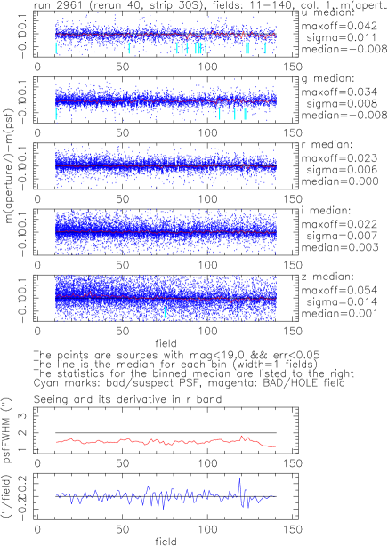
Figure 1: An example of output from the SDSS photometric assurance pipeline runQA. The top five panels show the difference between aperture and PSF magnitudes of stars brighter than $m\sim$19, as a function of time (1 field = 36 sec), for five SDSS bands. The statistics for medians, evaluated for each field, are shown next to each panel (maxoff is the maximum deviation from zero, sigma is the rms scatter). The vertical lines in each panel mark bad fields. The bottom two panels show the image quality in the $r$ band (FWHM and its time derivative) as a function of time.

3.2 Photometric zeropoint calibration

Data from each camera column, and for a given run, are independently calibrated. The calibration pipeline nfcalib reports the rms (dis)agreement, which is typically $\sim$0.02 mag (the core width, but the distribution is not necessarily Gaussian). There are usually several calibration patches for a given run, which are separated by of order an hour of scanning time. Thus, any changes in atmospheric transparency, or other conditions affecting the photometric sensitivity, may not be recognized on shorter timescales. In addition, the stability of photometric calibration across the sky is sensitive to systematic errors in the calibration star network. Hence, it is desirable to have an independent estimate of the stability of photometric calibration across the sky, as well as of its behavior on short time scales (say, a few minutes).

A dense network of calibration stars ($\ga$100 stars per deg²) across the sky, accurate to $\sim$0.01 mag, in five SDSS bands, which could be used for an independent verification of SDSS photometric calibration, does not yet exist. Fortunately, the distribution of stars in SDSS color-color diagrams seems fairly stable across the sky ($<$0.01 mag), and offers an indirect but powerful test of photometric zeropoint calibration.

3.2.1 Definition of the stellar locus in the SDSS photometric system

The majority of stars detected by SDSS are on the main sequence ($>$98%, Finlator et al. 2001, Helmi et al. 2002). They form a well defined sequence, usually referred to as a “stellar locus”, in color-color diagrams (Lenz et al, 1998, Fan 1999, Smolčić et al. 2004). The particular morphology displayed by the stellar locus can be used to measure whether it is “in the same place” for independently calibrated data.

The methodology used to derive the principal colors which track the position of the stellar locus is described in Helmi et al. (2002). Briefly, two principal axes, $P_{1}$ and $P_{2}$, are defined along the locus and perpendicular to the locus, for the appropriately chosen parts of the locus, and in three color-color planes spanned by SDSS photometric system. The color perpendicular to the locus, $P_{2}$, is adjusted for a small dependence on apparent magnitude ($<$0.01 mag/mag), to obtain $P^{\prime}_{2}$, which is then used for high-precision tracking of the locus position.

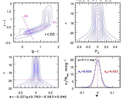
Figure 2: An example of the definition of principal color axes in color-color diagrams. The top left panel shows the $r-i$ vs. $g-r$ color-color diagram, with the $P_{1}$ axis along the blue part of the locus, and $P_{2}$ perpendicular to the locus. The top right panel shows the $P_{2}$ color as a function of $r$ magnitude. The $w$ principal color, shown as a function of $r$ magnitude in the bottom left panel, is obtained by correcting $P_{2}$ for its small dependence on $r$, and renormalizing it such that $w$ error (random, not systematic) is comparable to the mean error in the $g$, $r$, and $i$ bands. The solid histogram in the bottom right panel shows the distribution of $w$ color for stars with $r<20$. The dashed histogram shows the distribution of $w$ color constructed with the mean of five measurements (i.e. five passes over a given region of sky). The distribution rms width decreases from 0.025 mag to 0.022 mag, which implies that single measurement error for the $w$ color is $\sim$0.01 mag, and that the intrinsic locus width in the $w$ direction is $\sim$0.02 mag.

There are four principal colors used by runQA: $s$ (the blue part of the locus in the $g$-$r$ vs. $u$-$g$ plane), $w$ (blue part in $r$-$i$ vs. $g$-$r$), $x$ (red part in $r$-$i$ vs. $g$-$r$), and $y$ (red part in $i$-$z$ vs. $r$-$i$). As an example, the definition and properties of the $w$ color are shown in Fig. 2. The principal colors are defined by the following linear combinations of magnitudes in the five SDSS bands:

$$P^{\prime}_{2}=A\,u+B\,g+C\,r+D\,i+E\,z+F,$$ (1)

and

$$P_{1}=A^{\prime}\,u+B^{\prime}\,g+C^{\prime}\,r+D^{\prime}\,i+E^{\prime}\,z+F^{\prime},$$ (2)

where $P^{\prime}_{2}=s,w,x,y$ are the principal colors perpendicular to the locus in a particular color-color diagram, and $P_{1}$ (for each $P^{\prime}_{2}$) are the corresponding principal axes along the locus. All the measurements are corrected for interstellar extinction using the Schlegel, Finkbeiner & Davis (1998) map (SFD). The adopted coefficients $A-F$ and $A^{\prime}-F^{\prime}$ are listed in Tables 1 and 2. Stars used for estimating the position of the stellar locus must not have processing flags BRIGHT, SATUR, and BLENDED set (see Stoughton et al. 2002 for more details about photo processing flags), and must also satisfy $r<r_{max}$ and $P_{1}^{min}<P_{1}<P_{1}^{max}$, with $r_{max}$, $P_{1}^{min}$ and $P_{1}^{max}$ for each principal color listed in Table 3. The typical width of the stellar locus (the rms distribution width for each principal color) is listed in the last column in Table 3.

Even at high galactic latitudes ($|b|>30$), the surface density of stars satisfying these criteria is sufficient for evaluating the mean of the principal colors with an error of $\sim 0.01$ mag per SDSS field (area of 0.032 deg²). The mean error values per SDSS field for each principal color are listed in Table 3 ($\sigma$). The principal colors are evaluated by runQA in four field wide bins, yielding errors twice as small as those listed in Table 3.

The achievable accuracy in the determination of the position of the stellar locus depends on the number of stars in the sample and the intrinsic locus width. While the measured locus width is broadened by photometric errors, its value is, nevertheless, dominated by the intrinsic distribution of stellar properties such as metallicity and surface gravity. This conclusion is based on a comparison of the locus width for a set of single measurements, and using the mean values for five measurements of the same stars (see the bottom right panel in Fig. 2). Although the latter data have much smaller measurement errors, the width of the distribution is not significantly decreased, showing that most of the observed width is intrinsic.

Table 1: The $P^{\prime}_{2}$=$s,w,x,y$ Principal Color Definitions

$P^{\prime}_{2}$	A	B	C	D	E	F
s	-0.249	0.794	-0.555	0.0	0.0	0.234
w	0.0	-0.227	0.792	-0.567	0.0	0.050
x	0.0	0.707	-0.707	0.0	0.0	-0.988
y	0.0	0.0	-0.270	0.800	-0.534	0.054

Table 2: The $P_{1}$ Principal Color Definitions for each $P^{\prime}_{2}$

$P^{\prime}_{2}$	A’	B’	C’	D’	E’	F’
s	0.910	-0.495	-0.415	0.0	0.0	-1.28
w	0.0	0.928	-0.556	-0.372	0.0	-0.425
x	0.0	0.0	1.0	-1.0	0.0	0.0
y	0.0	0.0	0.895	-0.448	-0.447	-0.600

Table 3: Additional Constraints for the Principal Color Definitions

$P^{\prime}_{2}$	$r_{max}$	$P_{1}^{min}$	$P_{1}^{max}$	$\sigma$ (mag)	width (mag)
s	19.0	-0.2	0.8	0.011	0.031
w	20.0	-0.2	0.6	0.006	0.025
x	19.0	0.8	1.6	0.021	0.042
y	19.5	0.1	1.2	0.008	0.023

3.2.2 The measurements of the position of the stellar locus

For each of the four principal colors, the runQA pipeline computes and reports the low-order distribution statistics (such as median, rms, and the fraction of 3$\sigma$ outliers), in graphical and tabular form. These statistics are used to evaluate the accuracy of photometric zeropoint calibration for each run/camera column combination, as well as to track photometric accuracy as a function of time. For example, in case of unrecognized non-gray atmospheric extinction variations, the position of the locus (the principal color medians) changes, too. When the PSF model is incorrect, the locus width (and typically the fraction of 3$\sigma$ outliers) increases. As an example, the behavior of the $w$ color as a function of time in one run is shown in Fig. 3. All instances where the median principal color, or principal color distribution width, are outside adopted boundaries are interpreted as fields with substandard photometry, and reported in a “field quality” table. The distributions of the median principal colors for 291 SDSS runs processed to date are shown in the left two panels in Fig. 4. The mean distribution widths are listed in the last column in Table 3.

In principle, the median principal colors could vary across the sky due to galactic structure and stellar population effects. In order to estimate the magnitude of such variations, we consider the rms scatter of the mean stellar locus position for six camera columns in a given run, and its distribution for all runs. This scatter should be insensitive to the exact position of the stellar locus because stellar population variations should not be significant on the camera’s angular scale of $\sim$2 degree. If the position of the stellar locus does not vary appreciably across the sky, then the median value of this rms scatter should be similar to the rms scatter of the median position of the stellar locus. We find this to be the case for all four principal colors (see the right two panels in Fig. 4). This agreement suggests that the variations in the median principal colors are dominated by the errors in photometric zeropoint calibration, although we can not exclude the possibility that the observed variations are at least partly due to galactic structure effects. Hence, the estimates of photometric zeropoint calibration errors presented here are upper limits, and the true calibration errors could be indeed somewhat smaller.

While SDSS is by design a high galactic latitude survey, there are imaging data that probe low galactic latitudes. We find that the method for tracking the position of the stellar locus described here starts to fail at latitudes below $|b|=10-15$ deg. The main reason is that nearby M dwarfs are not behind all the dust implied by the SFD extinction map. As the extinction increases towards the Galactic plane, this fact becomes increasingly important, and induces a shift in the position of the stellar locus. While it may be possible to account for this effect by adopting a photometric parallax relation for M dwarfs, and assuming a dust distribution model, this possibility has not yet been quantitatively investigated.

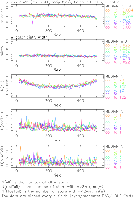
Figure 3: An example of the stellar locus position (top), rms width (second panel from top), and tail behavior (the bottom two panels) as a function of time, for the six camera columns. The “tails” are defined as 2$\sigma$ outliers.

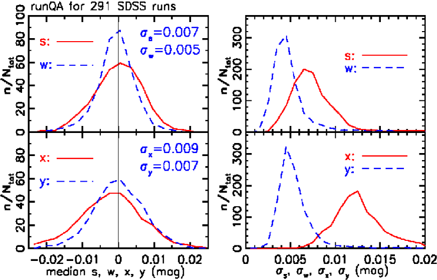
Figure 4: The two left panels show the distributions of the median for the four principal colors (which measure the position of the stellar locus position), evaluated for 291 SDSS runs processed to date ($\sigma$ values are the distribution rms widths). The two right panels show the distributions of the rms scatter of the mean stellar locus position for six camera columns in a given run. The fact that the median values of this rms scatter are similar to the widths of the distributions shown in the two left panels demonstrates that the observed variations in the locus position are dominated by the errors in photometric zeropoint calibration.

3.2.3 The distributions of SDSS photometric calibration errors

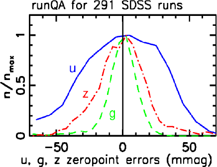
Figure 5: The distribution of the systematic errors in photometric zeropoint for the $u$, $g$, and $z$ bands (the distributions for the $r$ and $i$ bands are similar to the $g$ band distribution). The distribution widths are $\sim 0.01$ mag in the $g$, $r$, and $i$ bands, 0.02 mag in the $z$ band, and 0.03 mag in the $u$ band.

The principal colors are insensitive to “gray” calibration errors (i.e. the same offset in all bands). In order to estimate the photometric zeropoint errors in each SDSS band, we use an ansatz motivated by the fact that these errors are typically the smallest in $g$, $r$ and $i$ bands, as indicated by the direct comparison with calibration stars. With an assumption that the errors in the $g$, $r$ and $i$ bands sum to zero, we compute the photometric zeropoint errors in each SDSS band by inverting the equations that define principal colors (by assuming that, instead, the $r$ band calibration errors are zero, one gets practically the same solutions, in particular, the $u$ band calibration error is about four times the offset in $s$ color).

Fig. 5 shows the distribution of inferred photometric zeropoint errors in three representative bands for 291 SDSS runs. The rms widths of these distributions are $\sim 0.01$ mag in the $g$, $r$, and $i$ bands, 0.02 mag in the $z$ band, and 0.03 mag in the $u$ band. We emphasize that these values apply to all processed SDSS runs – those with the worst calibration errors are excluded from the public data releases (the rms widths remain similar to the above listed values).

4 Astrometric calibration, star/galaxy classification, flatfield vectors, etc.

Additional tasks performed by the runQA pipeline include an analysis of the accuracy of relative astrometric calibration (transformations between positions measurements in the five SDSS bands), and analysis of median principal colors as a function of chip position to track the flatfield vector accuracy. For example, the latter was used to discover that (and to derive appropriate corrections for) the shapes of the flatfield vectors vary with time (on a scale of several dark runs), up to 20% in some $u$ band chips.

A similar pipeline, matchQA, compares two observations of the same area on the sky. It quantifies the repeatability of SDSS measurements, and provides a handle on the sensitivity of measured parameters to varying observing conditions (such as seeing and sky brightness). For example, its outputs demonstrate that the star/galaxy classification is typically repeatable at the $>99\%$ level at the bright end ($r<20$), and at the $>95\%$ level for sources as faint as $r=21.5$. Furthermore, a direct comparison of photometry for multiply observed sources demonstrates that not only are the (random) photometric errors small ($\sim$0.02 mag), but they themselves are accurately determined by the photometric pipeline (see Fig. 2 in Ivezić et al. 2003). Furthermore, the tails of the photometric error distribution are well controlled and practically Gaussian (see Fig. 3 in Ivezić et al. 2003).

5 Discussion

SDSS is an excellent example of a modern astronomical survey – it produces unprecedentedly accurate data ($\sim$10 times more accurate than previous large-scale optical sky surveys, such as POSS, see Sesar et al. 2004), with a large peak data rate (20 GB/hr), and is built upon sophisticated data acquisition, processing and distribution systems ($\sim$million lines of code), that were developed by a large number of collaborators ($\sim$50). The success of SDSS provides encouragement that even more ambitious surveys, such as LSST (Tyson 2002), which is expected to produce and immediately process 20 TB of data per observing night, may also be successful endeavors.

SDSS also demonstrated, as described in this contribution, that a quantitative and efficient data quality assessment can be designed and implemented even when the “true answers” are not known for individual measurements. However, the method described here is not universal – it applies only to the wavelength range accessed by SDSS (0.3–1 $\mu$m), and to Galactic latitudes more than $\sim$15 degree from the galactic plane. Despite these shortcomings, it is a robust automated method that tracks the accuracy of SDSS photometric zeropoint calibration to better than 0.01 mag. We estimated, using this method, that typical photometric zeropoint calibration errors for SDSS imaging data are not larger than $\sim 0.01$ mag in the $g$, $r$, and $i$ bands, 0.02 mag in the $z$ band, and 0.03 mag in the $u$ band.