Relativistic magnetohydrodynamics in the early Universe

Abstract

We review the conservation laws of magnetohydrodynamics (MHD) in an expanding homogeneous and isotropic Universe that can be applied to the study of early Universe physics during the epoch of radiation domination. The conservation laws for a conducting perfect fluid with relativistic bulk velocities in an expanding background are presented, extending previous results that apply in the limit of subrelativistic bulk motion. Furthermore, it is shown that the subrelativistic limit presents new corrections that have not been considered in previous work. Imperfect relativistic fluids are briefly described but their detailed study is not included in this work. We review the propagation of sound waves, Alfvén waves, and magnetosonic waves, as well as the Boris correction for relativistic Alfvén speeds. This review is an extension, including new results, of part of the lectures presented at the minicourse “Simulations of Early Universe Magnetohydrodynamics” lectured by A. Roper Pol and J. Schober at EPFL, as part of the six-week program “Generation, evolution, and observations of cosmological magnetic fields” at the Bernoulli Center in May 2024.

Keywords: magnetohydrodynamics, early universe, cosmology

Relativistic magnetohydrodynamics in the early Universe

1 Introduction

In this work, magnetohydrodynamic (MHD) perturbations in the early Universe are reviewed, described in general relativity over the Friedmann–Lemaître–Robertson–Walker (FLRW) background metric for a homogeneous and isotropic expanding Universe, according to the cosmological principle. As the focus is on the relativistic MHD description, only a minimal review on cosmology is given in section 2. We refer the reader to textbook references on cosmology, for example [1, 2], or [3] for a recent textbook. For extended work on perfect fluids and electromagnetism in general relativity, the literature is extensive; we recommend the reader the following textbook references [4, 5, 6, 7, 8, 9].

The MHD equations in a cosmological expanding background have been studied following the pioneering work of [10, 11, 12]. In particular, the MHD equations during the radiation-dominated era in the early Universe have been considered, for example, to study the evolution of primordial magnetic fields [10, 13, 14, 15, 16, 17, 18, 19, 20, 21, 22, 23, 24, 25, 26, 27, 28, 29, 30], the production of gravitational waves (GWs) from MHD turbulence [31, 32, 33, 34, 35, 36, 37, 38, 39, 40], and the chiral magnetic effect [41, 42, 43, 44, 45, 46, 47]. Excellent reviews on the generation, evolution, and observational signatures of primordial magnetic fields exist in the literature (cf. [20, 23, 48]). The aim of the present work is to review the MHD equations in an expanding background, extending previous work to relativistic bulk motion and presenting new results on the fully relativistic description of perfect fluids and resistive MHD. In particular, we also show that previous work assuming the $\gamma^{2}=(1-u^{2})^{-1}\approx 1$ limit in the subrelativistic regime (see, e.g., [10, 20, 23] and references therein) ignores time derivatives of $\gamma$, which can lead to terms of order $u^{2}/\ell$, being $\ell$ a characteristic fluid length scale, similar to the convective derivative term $(\mathchoice{\mbox{\boldmath$\displaystyle u$}}{\mbox{\boldmath$\textstyle u$}}{\mbox{\boldmath$\scriptstyle u$}}{\mbox{\boldmath$\scriptscriptstyle u$}}{}\cdot\mathchoice{\mbox{\boldmath$\displaystyle\nabla$}}{\mbox{\boldmath$\textstyle\nabla$}}{\mbox{\boldmath$\scriptstyle\nabla$}}{\mbox{\boldmath$\scriptscriptstyle\nabla$}}{})\mathchoice{\mbox{\boldmath$\displaystyle u$}}{\mbox{\boldmath$\textstyle u$}}{\mbox{\boldmath$\scriptstyle u$}}{\mbox{\boldmath$\scriptscriptstyle u$}}{}$. Therefore, some of these terms should not be ignored in a non-linear description of subrelativistic hydrodynamics or MHD.

Some of the results in this review were covered in the lectures presented during the EPFL course “Simulations of Early Universe Magnetohydrodynamics,” in particular the theory lectures on “MHD in an expanding Universe,” lectured by one of the authors, as a part of the six-week program “Generation, evolution, and observations of cosmological magnetic fields” at the Bernoulli Center.

With the growing interest in studying the evolution of primordial magnetic fields, fluid perturbations, and GWs, among others, in the early Universe, the results presented in this review can be used for a broad range of cosmological applications. Many of these studies have been performed in the subrelativistic limit using the open-source Pencil Code [49], adapted to a radiation-dominated fluid with an equation of state $p=c_{\rm s}^{2}\rho$, where $p$ is the pressure, $\rho$ is the total energy density, and $c_{\rm s}^{2}=1/3$ the speed of sound, following the pioneer work of [10]. Current developments for including relativistic MHD in an expanding background in Pencil Code are in progress by the authors and collaborators. In addition, the open-source ${\cal C}$osmo${\cal L}$attice [50, 51] is also being developed to include an MHD description for early Universe studies [52, 53]. In the current review, we present the theoretical framework for MHD studies in the early Universe going beyond the currently studied subrelativisitc limit of bulk fluid motion, and present new results that also lead to some corrections in the subrelativistic limit that should be addressed in future studies.

In section 2, the FLRW geometry of an isotropic and homogeneous expanding Universe is reviewed. This is considered to describe the metric tensor over which the MHD conservation laws are studied. The perturbations on the metric tensor induced by the velocity and magnetic fields are assumed to be subdominant, such that we can ignore backreaction of the metric tensor perturbations in the MHD equations. In section 3, the conservation laws of a fully relativistic perfect fluid in the absence of electromagnetic fields in an expanding Universe are presented, briefly describing imperfect fluids (with viscous and heat transfer contributions) in section 3.6. Sound waves are studied in section 3.5. In section 4, Maxwell equations in an expanding background are reviewed, introducing the definitions of comoving electromagnetic fields and current density (section 4.2), together with the covariant formulation of the generalized Ohm’s law (section 4.3), required to describe the current density in relativistic fluids. In section 5, the MHD conservation laws for a relativistic charged fluid are described. Linear MHD perturbations in an expanding Universe are studied in sections 5.5–5.7. In section 5.6, the Boris correction is introduced, which allows to correct the Alfvén speed when it becomes relativistic, even in the subrelativistic limit of bulk flow velocities. We conclude in section 6.

In the present work, contributions from neutrino and electron free streaming below the Silk damping scales are ignored. They have been studied in the literature (see [11, 12] for pioneering work). The Silk damping scale becomes larger towards the onset of matter domination in the early Universe and, hence, it needs to be taken into account to study the correct evolution of large-scale primordial magnetic fields across the early Universe, especially through the epoch of recombination. The effect of viscosity in this work is only presented using the Navier-Stokes covariant description [1, 11, 12]. It is known that this description leads to acausal fluid perturbations and a relativistic description of viscous hydrodynamics is an active field of research (see, e.g., the review in [54]). For the sake of simplicity, a fully relativistic causal description is not included in the present review. At high energies, asymmetries between left and right-handed particles would lead to a chiral induced current [55] that can produce vorticity and drive magnetic fields in processes known as the chiral vortical and magnetic effects. The latter effect has been studied in the context of primordial magnetic fields using MHD simulations (see [41, 42, 43] for pioneering work). Chiral effects are also ignored in this work.

Conventions and notation

Natural units with $c=1$ and Heaviside-Lorentz units for electromagnetic fields are considered along the text. In these units, the Maxwell equations are

$$\partial_{t}\mathchoice{\mbox{\boldmath$\displaystyle E$}}{\mbox{\boldmath$\textstyle E$}}{\mbox{\boldmath$\scriptstyle E$}}{\mbox{\boldmath$\scriptscriptstyle E$}}{}=\mathchoice{\mbox{\boldmath$\displaystyle\nabla$}}{\mbox{\boldmath$\textstyle\nabla$}}{\mbox{\boldmath$\scriptstyle\nabla$}}{\mbox{\boldmath$\scriptscriptstyle\nabla$}}{}\times\mathchoice{\mbox{\boldmath$\displaystyle B$}}{\mbox{\boldmath$\textstyle B$}}{\mbox{\boldmath$\scriptstyle B$}}{\mbox{\boldmath$\scriptscriptstyle B$}}{}-\mathchoice{\mbox{\boldmath$\displaystyle J$}}{\mbox{\boldmath$\textstyle J$}}{\mbox{\boldmath$\scriptstyle J$}}{\mbox{\boldmath$\scriptscriptstyle J$}}{}\,,\quad\mathchoice{\mbox{\boldmath$\displaystyle\nabla$}}{\mbox{\boldmath$\textstyle\nabla$}}{\mbox{\boldmath$\scriptstyle\nabla$}}{\mbox{\boldmath$\scriptscriptstyle\nabla$}}{}\cdot\mathchoice{\mbox{\boldmath$\displaystyle E$}}{\mbox{\boldmath$\textstyle E$}}{\mbox{\boldmath$\scriptstyle E$}}{\mbox{\boldmath$\scriptscriptstyle E$}}{}=\rho_{e}\,,\quad\partial_{t}\mathchoice{\mbox{\boldmath$\displaystyle B$}}{\mbox{\boldmath$\textstyle B$}}{\mbox{\boldmath$\scriptstyle B$}}{\mbox{\boldmath$\scriptscriptstyle B$}}{}=-\mathchoice{\mbox{\boldmath$\displaystyle\nabla$}}{\mbox{\boldmath$\textstyle\nabla$}}{\mbox{\boldmath$\scriptstyle\nabla$}}{\mbox{\boldmath$\scriptscriptstyle\nabla$}}{}\times\mathchoice{\mbox{\boldmath$\displaystyle E$}}{\mbox{\boldmath$\textstyle E$}}{\mbox{\boldmath$\scriptstyle E$}}{\mbox{\boldmath$\scriptscriptstyle E$}}{}\,,\quad\mathchoice{\mbox{\boldmath$\displaystyle\nabla$}}{\mbox{\boldmath$\textstyle\nabla$}}{\mbox{\boldmath$\scriptstyle\nabla$}}{\mbox{\boldmath$\scriptscriptstyle\nabla$}}{}\cdot\mathchoice{\mbox{\boldmath$\displaystyle B$}}{\mbox{\boldmath$\textstyle B$}}{\mbox{\boldmath$\scriptstyle B$}}{\mbox{\boldmath$\scriptscriptstyle B$}}{}=0\,.$$ (1.1)

In general, $t$ and $\tau$ are used for cosmic and conformal time, respectively. Derivatives with respect to $t$ and $\tau$ are denoted by a dot (e.g., $\dot{a}$) and a prime (e.g., $a^{\prime}$), respectively. The early Universe geometry is described by the homogeneous, isotropic, and spatially flat Friedmann-Lemaître-Robertson-Walker (FLRW) metric tensor, $g_{\mu\nu}=a^{2}\eta_{\mu\nu}$ with $\eta_{\mu\nu}=m\,{\rm diag}\{-1,1,1,1\}$ being the Minkowski space-metric tensor. We will assume that the MHD perturbations are small compared to the background, such that their effect on the metric does not feedback into the MHD equations. The signature is $m\,(-\,+\,+\,+)$, such that $m=\pm 1$ allows to keep track of the signature-dependent quantities. Taking $m=1$, space-time intervals are spacelike and it is more commonly used in general relativity, for example in [4, 5, 8], while $m=-1$ yields timelike intervals and it is more common in particle physics and cosmology, for example in [56, 3]. In section 2, a generic signature will be considered, while in the remaining of the text, when the equations of motion are computed, $m=1$ will be used for compactness of the calculations as the resulting equations of motion are not affected by the signature choice.

In most of the text, the coordinates are $X^{0}=\tau$ and $X^{i}=x^{i}$ with $x^{i}$ being the comoving space coordinates. Only in section 2, $X^{0}$ is allowed to be a generic $\alpha$-time, such that $a^{\alpha}{\rm\,d}\tau_{\alpha}={\rm\,d}t$, which reduces to cosmic or conformal when $\alpha=0$ or 1, respectively.

Relativistic MHD equations in an expanding Universe

For the impatient reader, let us present the set of relativistic MHD equations describing the evolution of the total energy density $\rho$ and the velocity field $\textstyle u$, found in the present work (see section 5), which, up to our knowledge, has not been considered in previous work:

$$\partial_{\tau}\ln\tilde{\rho}=-\frac{1+c_{\rm s}^{2}}{1-c_{\rm s}^{2}u^{2}}\biggl{[}\mathchoice{\mbox{\boldmath$\displaystyle\nabla$}}{\mbox{\boldmath$\textstyle\nabla$}}{\mbox{\boldmath$\scriptstyle\nabla$}}{\mbox{\boldmath$\scriptscriptstyle\nabla$}}{}\cdot\mathchoice{\mbox{\boldmath$\displaystyle u$}}{\mbox{\boldmath$\textstyle u$}}{\mbox{\boldmath$\scriptstyle u$}}{\mbox{\boldmath$\scriptscriptstyle u$}}{}+\frac{1-c_{\rm s}^{2}}{1+c_{\rm s}^{2}}\,\bigl{(}\mathchoice{\mbox{\boldmath$\displaystyle u$}}{\mbox{\boldmath$\textstyle u$}}{\mbox{\boldmath$\scriptstyle u$}}{\mbox{\boldmath$\scriptscriptstyle u$}}{}\cdot\mathchoice{\mbox{\boldmath$\displaystyle\nabla$}}{\mbox{\boldmath$\textstyle\nabla$}}{\mbox{\boldmath$\scriptstyle\nabla$}}{\mbox{\boldmath$\scriptscriptstyle\nabla$}}{}\bigr{)}\ln\tilde{\rho}+{\cal H}\,\frac{3c_{\rm s}^{2}-1}{1+c_{\rm s}^{2}}(1+u^{2})\biggr{]}$$

$$+\frac{1}{1-c_{\rm s}^{2}u^{2}}\biggl{[}\frac{\tilde{f}_{\rm tot}^{0}}{\tilde{\rho}}(1+u^{2})-2\,\frac{\mathchoice{\mbox{\boldmath$\displaystyle u$}}{\mbox{\boldmath$\textstyle u$}}{\mbox{\boldmath$\scriptstyle u$}}{\mbox{\boldmath$\scriptscriptstyle u$}}{}\cdot\mathchoice{\mbox{\boldmath$\displaystyle\tilde{f}$}}{\mbox{\boldmath$\textstyle\tilde{f}$}}{\mbox{\boldmath$\scriptstyle\tilde{f}$}}{\mbox{\boldmath$\scriptscriptstyle\tilde{f}$}}{}_{\rm tot}}{\tilde{\rho}}\biggr{]}\,,$$ (1.2a)

$$\partial_{\tau}\mathchoice{\mbox{\boldmath$\displaystyle u$}}{\mbox{\boldmath$\textstyle u$}}{\mbox{\boldmath$\scriptstyle u$}}{\mbox{\boldmath$\scriptscriptstyle u$}}{}+\bigl{(}\mathchoice{\mbox{\boldmath$\displaystyle u$}}{\mbox{\boldmath$\textstyle u$}}{\mbox{\boldmath$\scriptstyle u$}}{\mbox{\boldmath$\scriptscriptstyle u$}}{}\cdot\mathchoice{\mbox{\boldmath$\displaystyle\nabla$}}{\mbox{\boldmath$\textstyle\nabla$}}{\mbox{\boldmath$\scriptstyle\nabla$}}{\mbox{\boldmath$\scriptscriptstyle\nabla$}}{}\bigr{)}\mathchoice{\mbox{\boldmath$\displaystyle u$}}{\mbox{\boldmath$\textstyle u$}}{\mbox{\boldmath$\scriptstyle u$}}{\mbox{\boldmath$\scriptscriptstyle u$}}{}=\frac{\mathchoice{\mbox{\boldmath$\displaystyle u$}}{\mbox{\boldmath$\textstyle u$}}{\mbox{\boldmath$\scriptstyle u$}}{\mbox{\boldmath$\scriptscriptstyle u$}}{}}{(1-c_{\rm s}^{2}u^{2})\gamma^{2}}\biggl{[}c_{\rm s}^{2}\,\mathchoice{\mbox{\boldmath$\displaystyle\nabla$}}{\mbox{\boldmath$\textstyle\nabla$}}{\mbox{\boldmath$\scriptstyle\nabla$}}{\mbox{\boldmath$\scriptscriptstyle\nabla$}}{}\cdot\mathchoice{\mbox{\boldmath$\displaystyle u$}}{\mbox{\boldmath$\textstyle u$}}{\mbox{\boldmath$\scriptstyle u$}}{\mbox{\boldmath$\scriptscriptstyle u$}}{}+c_{\rm s}^{2}\frac{1-c_{\rm s}^{2}}{1+c_{\rm s}^{2}}(\mathchoice{\mbox{\boldmath$\displaystyle u$}}{\mbox{\boldmath$\textstyle u$}}{\mbox{\boldmath$\scriptstyle u$}}{\mbox{\boldmath$\scriptscriptstyle u$}}{}\cdot\mathchoice{\mbox{\boldmath$\displaystyle\nabla$}}{\mbox{\boldmath$\textstyle\nabla$}}{\mbox{\boldmath$\scriptstyle\nabla$}}{\mbox{\boldmath$\scriptscriptstyle\nabla$}}{})\ln\tilde{\rho}+{\cal H}(3c_{\rm s}^{2}-1)-\frac{\tilde{f}_{\rm tot}^{0}}{\tilde{\rho}}\biggr{]}$$

$$+\frac{2\,\mathchoice{\mbox{\boldmath$\displaystyle u$}}{\mbox{\boldmath$\textstyle u$}}{\mbox{\boldmath$\scriptstyle u$}}{\mbox{\boldmath$\scriptscriptstyle u$}}{}\,c_{\rm s}^{2}}{(1+c_{\rm s}^{2})(1-c_{\rm s}^{2}u^{2})}\,\frac{\mathchoice{\mbox{\boldmath$\displaystyle u$}}{\mbox{\boldmath$\textstyle u$}}{\mbox{\boldmath$\scriptstyle u$}}{\mbox{\boldmath$\scriptscriptstyle u$}}{}\cdot\mathchoice{\mbox{\boldmath$\displaystyle\tilde{f}$}}{\mbox{\boldmath$\textstyle\tilde{f}$}}{\mbox{\boldmath$\scriptstyle\tilde{f}$}}{\mbox{\boldmath$\scriptscriptstyle\tilde{f}$}}{}_{\rm tot}}{\tilde{\rho}\gamma^{2}}-\frac{c_{\rm s}^{2}}{1+c_{\rm s}^{2}}\frac{\mathchoice{\mbox{\boldmath$\displaystyle\nabla$}}{\mbox{\boldmath$\textstyle\nabla$}}{\mbox{\boldmath$\scriptstyle\nabla$}}{\mbox{\boldmath$\scriptscriptstyle\nabla$}}{}\ln\tilde{\rho}}{\gamma^{2}}+\frac{1}{1+c_{\rm s}^{2}}\,\frac{\mathchoice{\mbox{\boldmath$\displaystyle\tilde{f}$}}{\mbox{\boldmath$\textstyle\tilde{f}$}}{\mbox{\boldmath$\scriptstyle\tilde{f}$}}{\mbox{\boldmath$\scriptscriptstyle\tilde{f}$}}{}_{\rm tot}}{\tilde{\rho}\gamma^{2}}\,,$$ (1.2b)

where $\tau$ corresponds to conformal time, $a$ is the scale factor, and ${\cal H}=a^{\prime}/a$ is the conformal Hubble rate. The velocity field $\textstyle u$ corresponds to the peculiar velocity with respect to the Hubble observer $\mathchoice{\mbox{\boldmath$\displaystyle u$}}{\mbox{\boldmath$\textstyle u$}}{\mbox{\boldmath$\scriptstyle u$}}{\mbox{\boldmath$\scriptscriptstyle u$}}{}={\rm\,d}\mathchoice{\mbox{\boldmath$\displaystyle x$}}{\mbox{\boldmath$\textstyle x$}}{\mbox{\boldmath$\scriptstyle x$}}{\mbox{\boldmath$\scriptscriptstyle x$}}{}/{\rm\,d}\tau$, i.e., comoving with the Universe expansion (see section 2.4). The comoving energy density and pressure are $\tilde{\rho}=a^{4}\rho$ and $\tilde{p}=a^{4}p$, respectively, where a constant equation of state is considered to describe the comoving pressure $\tilde{p}=c_{\rm s}^{2}\tilde{\rho}$. Comoving variables and spatial coordinates $\textstyle x$, together with conformal time, are chosen to exploit the conformal invariance of the equations for a radiation-dominated fluid with $c_{\rm s}^{2}=1/3$ [10] (see section 3 and, in particular, section 3.2), as can be seen by the fact that no dependence on $a$ is left in (1.2a) and (1.2b) when $c_{\rm s}^{2}=1/3$. Even though the equations become conformally flat, the inclusion of a relativistic equation of state $c_{\rm s}^{2}\sim{\cal O}(1)$ requires to modify the MHD equations with respect to a fluid composed by dust particles $c_{\rm s}^{2}\ll 1$, even in the limit of subrelativistic bulk velocities, $u^{2}\ll 1$ [10]. Hence, the usual results for classical MHD systems, with $c_{\rm s}^{2}\ll 1$ and ignoring the Universe expansion, need to be adapted to take these modifications into account.

The comoving four-force $\tilde{f}^{\mu}_{\rm tot}=a^{6}f^{\mu}_{\rm tot}$ can correspond to any force applied to the fluid and it appears from additional contributions to the stress-energy tensor than those corresponding to a perfect fluid $T^{\mu\nu}_{\rm pf}$. In particular, we study in section 3.6 the inclusion of out-of-local-thermal-equilibrium effects like viscosity or heat transfer by incorporating a deviatoric tensor $\Pi^{\mu\nu}$, such that $T^{\mu\nu}=T^{\mu\nu}_{\rm pf}-\Pi^{\mu\nu}$, yielding, for example, a viscous force $f^{\nu}_{\rm visc}=\partial_{\mu}\Pi^{\mu\nu}$. The inclusion of electromagnetic forces to the fluid is required for the study of MHD (see section 5). It can be described by incorporating the electromagnetic stress-energy tensor, $T^{\mu\nu}\to T^{\mu\nu}+T^{\mu\nu}_{\rm EM}$, which yields the Lorentz force $f^{\nu}_{\rm EM}=-\partial_{\mu}T^{\mu\nu}_{\rm EM}$ (see section 5.2). When electromagnetic fields are included, (1.2a) and (1.2b) have to be solved together with Maxwell equations in an expanding background, which can be expressed for the Hubble observer in the following way (using the temporal or Weyl gauge $A_{0}=0$),

$$\partial_{\tau}\mathchoice{\mbox{\boldmath$\displaystyle A$}}{\mbox{\boldmath$\textstyle A$}}{\mbox{\boldmath$\scriptstyle A$}}{\mbox{\boldmath$\scriptscriptstyle A$}}{}=-\mathchoice{\mbox{\boldmath$\displaystyle\tilde{E}$}}{\mbox{\boldmath$\textstyle\tilde{E}$}}{\mbox{\boldmath$\scriptstyle\tilde{E}$}}{\mbox{\boldmath$\scriptscriptstyle\tilde{E}$}}{}\,,\quad\partial_{\tau}\mathchoice{\mbox{\boldmath$\displaystyle\tilde{E}$}}{\mbox{\boldmath$\textstyle\tilde{E}$}}{\mbox{\boldmath$\scriptstyle\tilde{E}$}}{\mbox{\boldmath$\scriptscriptstyle\tilde{E}$}}{}=\mathchoice{\mbox{\boldmath$\displaystyle\nabla$}}{\mbox{\boldmath$\textstyle\nabla$}}{\mbox{\boldmath$\scriptstyle\nabla$}}{\mbox{\boldmath$\scriptscriptstyle\nabla$}}{}\times\mathchoice{\mbox{\boldmath$\displaystyle\tilde{B}$}}{\mbox{\boldmath$\textstyle\tilde{B}$}}{\mbox{\boldmath$\scriptstyle\tilde{B}$}}{\mbox{\boldmath$\scriptscriptstyle\tilde{B}$}}{}-\mathchoice{\mbox{\boldmath$\displaystyle\tilde{J}$}}{\mbox{\boldmath$\textstyle\tilde{J}$}}{\mbox{\boldmath$\scriptstyle\tilde{J}$}}{\mbox{\boldmath$\scriptscriptstyle\tilde{J}$}}{}\,,\quad\mathchoice{\mbox{\boldmath$\displaystyle\nabla$}}{\mbox{\boldmath$\textstyle\nabla$}}{\mbox{\boldmath$\scriptstyle\nabla$}}{\mbox{\boldmath$\scriptscriptstyle\nabla$}}{}\cdot\mathchoice{\mbox{\boldmath$\displaystyle\tilde{E}$}}{\mbox{\boldmath$\textstyle\tilde{E}$}}{\mbox{\boldmath$\scriptstyle\tilde{E}$}}{\mbox{\boldmath$\scriptscriptstyle\tilde{E}$}}{}=\tilde{J}^{0}\,,$$ (1.2c)

where $\textstyle\tilde{E}$, $\textstyle\tilde{B}$, and $\textstyle\tilde{J}$ correspond to the comoving electric, magnetic, and current density fields, and $\tilde{J}^{0}$ is the temporal component of the four-current (see section 4).

MHD equations in the limit of subrelativistic bulk motion

In the limit of subrelativistic bulk motion, $u^{2}\ll 1$, which has been considered in previous literature, (1.2a) and (1.2b) reduce to

$$\partial_{\tau}\ln\tilde{\rho}\,=-(1+c_{\rm s}^{2})\,\mathchoice{\mbox{\boldmath$\displaystyle\nabla$}}{\mbox{\boldmath$\textstyle\nabla$}}{\mbox{\boldmath$\scriptstyle\nabla$}}{\mbox{\boldmath$\scriptscriptstyle\nabla$}}{}\cdot\mathchoice{\mbox{\boldmath$\displaystyle u$}}{\mbox{\boldmath$\textstyle u$}}{\mbox{\boldmath$\scriptstyle u$}}{\mbox{\boldmath$\scriptscriptstyle u$}}{}-(1-c_{\rm s}^{2})(\mathchoice{\mbox{\boldmath$\displaystyle u$}}{\mbox{\boldmath$\textstyle u$}}{\mbox{\boldmath$\scriptstyle u$}}{\mbox{\boldmath$\scriptscriptstyle u$}}{}\cdot\mathchoice{\mbox{\boldmath$\displaystyle\nabla$}}{\mbox{\boldmath$\textstyle\nabla$}}{\mbox{\boldmath$\scriptstyle\nabla$}}{\mbox{\boldmath$\scriptscriptstyle\nabla$}}{})\ln\tilde{\rho}+\frac{\tilde{f}_{0}}{\tilde{\rho}}-\frac{2\,\mathchoice{\mbox{\boldmath$\displaystyle u$}}{\mbox{\boldmath$\textstyle u$}}{\mbox{\boldmath$\scriptstyle u$}}{\mbox{\boldmath$\scriptscriptstyle u$}}{}\cdot\mathchoice{\mbox{\boldmath$\displaystyle\tilde{f}$}}{\mbox{\boldmath$\textstyle\tilde{f}$}}{\mbox{\boldmath$\scriptstyle\tilde{f}$}}{\mbox{\boldmath$\scriptscriptstyle\tilde{f}$}}{}_{\rm tot}}{\tilde{\rho}}-{\cal H}\,(3c_{\rm s}^{2}-1)\,,$$ (1.2da)

$$\partial_{\tau}\mathchoice{\mbox{\boldmath$\displaystyle u$}}{\mbox{\boldmath$\textstyle u$}}{\mbox{\boldmath$\scriptstyle u$}}{\mbox{\boldmath$\scriptscriptstyle u$}}{}+(\mathchoice{\mbox{\boldmath$\displaystyle u$}}{\mbox{\boldmath$\textstyle u$}}{\mbox{\boldmath$\scriptstyle u$}}{\mbox{\boldmath$\scriptscriptstyle u$}}{}\cdot\mathchoice{\mbox{\boldmath$\displaystyle\nabla$}}{\mbox{\boldmath$\textstyle\nabla$}}{\mbox{\boldmath$\scriptstyle\nabla$}}{\mbox{\boldmath$\scriptscriptstyle\nabla$}}{})\,\mathchoice{\mbox{\boldmath$\displaystyle u$}}{\mbox{\boldmath$\textstyle u$}}{\mbox{\boldmath$\scriptstyle u$}}{\mbox{\boldmath$\scriptscriptstyle u$}}{}=\mathchoice{\mbox{\boldmath$\displaystyle u$}}{\mbox{\boldmath$\textstyle u$}}{\mbox{\boldmath$\scriptstyle u$}}{\mbox{\boldmath$\scriptscriptstyle u$}}{}\,\biggl{[}c_{\rm s}^{2}\,\mathchoice{\mbox{\boldmath$\displaystyle\nabla$}}{\mbox{\boldmath$\textstyle\nabla$}}{\mbox{\boldmath$\scriptstyle\nabla$}}{\mbox{\boldmath$\scriptscriptstyle\nabla$}}{}\cdot\mathchoice{\mbox{\boldmath$\displaystyle u$}}{\mbox{\boldmath$\textstyle u$}}{\mbox{\boldmath$\scriptstyle u$}}{\mbox{\boldmath$\scriptscriptstyle u$}}{}+c_{\rm s}^{2}\,\frac{1-c_{\rm s}^{2}}{1+c_{\rm s}^{2}}(\mathchoice{\mbox{\boldmath$\displaystyle u$}}{\mbox{\boldmath$\textstyle u$}}{\mbox{\boldmath$\scriptstyle u$}}{\mbox{\boldmath$\scriptscriptstyle u$}}{}\cdot\mathchoice{\mbox{\boldmath$\displaystyle\nabla$}}{\mbox{\boldmath$\textstyle\nabla$}}{\mbox{\boldmath$\scriptstyle\nabla$}}{\mbox{\boldmath$\scriptscriptstyle\nabla$}}{})\ln\tilde{\rho}-\frac{\tilde{f}_{0}}{\tilde{\rho}}+\frac{2c_{\rm s}^{2}}{(1+c_{\rm s}^{2})\tilde{\rho}}\,\mathchoice{\mbox{\boldmath$\displaystyle u$}}{\mbox{\boldmath$\textstyle u$}}{\mbox{\boldmath$\scriptstyle u$}}{\mbox{\boldmath$\scriptscriptstyle u$}}{}\cdot\mathchoice{\mbox{\boldmath$\displaystyle\tilde{f}$}}{\mbox{\boldmath$\textstyle\tilde{f}$}}{\mbox{\boldmath$\scriptstyle\tilde{f}$}}{\mbox{\boldmath$\scriptscriptstyle\tilde{f}$}}{}_{\rm tot}\biggr{]}$$

$$+\mathchoice{\mbox{\boldmath$\displaystyle u$}}{\mbox{\boldmath$\textstyle u$}}{\mbox{\boldmath$\scriptstyle u$}}{\mbox{\boldmath$\scriptscriptstyle u$}}{}\,{\cal H}\,(3c_{\rm s}^{2}-1)-\frac{c_{\rm s}^{2}}{1+c_{\rm s}^{2}}\mathchoice{\mbox{\boldmath$\displaystyle\nabla$}}{\mbox{\boldmath$\textstyle\nabla$}}{\mbox{\boldmath$\scriptstyle\nabla$}}{\mbox{\boldmath$\scriptscriptstyle\nabla$}}{}\ln\tilde{\rho}+\frac{\mathchoice{\mbox{\boldmath$\displaystyle\tilde{f}$}}{\mbox{\boldmath$\textstyle\tilde{f}$}}{\mbox{\boldmath$\scriptstyle\tilde{f}$}}{\mbox{\boldmath$\scriptscriptstyle\tilde{f}$}}{}_{\rm tot}}{(1+c_{\rm s}^{2})\tilde{\rho}}\,.$$ (1.2db)

We note that when $c_{\rm s}^{2}\sim{\cal O}(1)$, an additional term proportional to $\mathchoice{\mbox{\boldmath$\displaystyle u$}}{\mbox{\boldmath$\textstyle u$}}{\mbox{\boldmath$\scriptstyle u$}}{\mbox{\boldmath$\scriptscriptstyle u$}}{}\,c_{\rm s}^{2}$ appears in the momentum equation, which does not appear in the usual MHD (i.e., in fluids predominantly composed by massive particles, with $c_{\rm s}^{2}\ll 1$), as well as modifications in some coefficients of the different terms that depend on $c_{\rm s}^{2}$. We note that this additional term can lead to the production of vorticity when $c_{\rm s}^{2}\sim{\cal O}(1)$, even in the absence of external forcing (i.e., for the modified Euler equations). Therefore, vorticity is no longer a topological invariant, as for the usual Euler equations when $c_{\rm s}^{2}\ll 1$ [9]. This has recently been pointed out in [57, 58] in Minkowski space-time, and extended to the relativistic regime in [59]. Therefore, even when $c_{\rm s}^{2}=1/3$ and the MHD equations are conformally flat, one needs to incorporate the additional terms that appear as a consequence of $c_{\rm s}^{2}\sim{\cal O}(1)$ in the system, leading to minor (but potentially relevant) deviations with respect to usual MHD. A Hubble friction term proportional to ${\cal H}\,(3c_{\rm s}^{2}-1)$ appears when $c_{\rm s}^{2}\neq 1/3$ in both the momentum and energy conservation equations as a consequence of the Universe expansion, breaking the conformal invariance of the equations. Note that in the subrelativistic limit, the Hubble-dependent term in the energy equation vanishes if one rescales $\tilde{\rho}=a^{3\,(1+c_{\rm s}^{2})}$, as it is shown in section 3. The terms $\tilde{f}_{0}$ and $\mathchoice{\mbox{\boldmath$\displaystyle u$}}{\mbox{\boldmath$\textstyle u$}}{\mbox{\boldmath$\scriptstyle u$}}{\mbox{\boldmath$\scriptscriptstyle u$}}{}\cdot\mathchoice{\mbox{\boldmath$\displaystyle\tilde{f}$}}{\mbox{\boldmath$\textstyle\tilde{f}$}}{\mbox{\boldmath$\scriptstyle\tilde{f}$}}{\mbox{\boldmath$\scriptscriptstyle\tilde{f}$}}{}_{\rm tot}$ correspond to energy dissipation and power exerted by the different forces to the fluid. In addition, we find that $\partial_{\tau}\gamma^{2}$, omitted in previous work (see, e.g., [10, 25, 32]), presents terms that are non-negligible even in the subrelativistic limit (see section 3 and, in particular, section 3.4), yielding a modification in the coefficient of $(\mathchoice{\mbox{\boldmath$\displaystyle u$}}{\mbox{\boldmath$\textstyle u$}}{\mbox{\boldmath$\scriptstyle u$}}{\mbox{\boldmath$\scriptscriptstyle u$}}{}\cdot\mathchoice{\mbox{\boldmath$\displaystyle\nabla$}}{\mbox{\boldmath$\textstyle\nabla$}}{\mbox{\boldmath$\scriptstyle\nabla$}}{\mbox{\boldmath$\scriptscriptstyle\nabla$}}{})\ln\tilde{\rho}$ in the energy equation [see (1.2da)] and in the coefficient of $\mathchoice{\mbox{\boldmath$\displaystyle u$}}{\mbox{\boldmath$\textstyle u$}}{\mbox{\boldmath$\scriptstyle u$}}{\mbox{\boldmath$\scriptscriptstyle u$}}{}\,(\mathchoice{\mbox{\boldmath$\displaystyle u$}}{\mbox{\boldmath$\textstyle u$}}{\mbox{\boldmath$\scriptstyle u$}}{\mbox{\boldmath$\scriptscriptstyle u$}}{}\cdot\mathchoice{\mbox{\boldmath$\displaystyle\nabla$}}{\mbox{\boldmath$\textstyle\nabla$}}{\mbox{\boldmath$\scriptstyle\nabla$}}{\mbox{\boldmath$\scriptscriptstyle\nabla$}}{})\ln\tilde{\rho}$ in the momentum equation [see (1.2db)].

2 Friedmann–Lemaître–Robertson–Walker background

At large distances in our universe, the distribution of galaxies becomes homogeneous and isotropic as we look farther away from us. This is known as the cosmological principle and its strongest observation evidence is the uniformity of the cosmic microwave background (CMB), with observed anisotropies in the CMB temperature being only of a few parts in $10^{5}$ [60]. Under the assumptions of homogeneity and isotropy, Einstein field equations have an exact solution, corresponding to the Friedmann–Lemaître–Robertson–Walker (FLRW) metric tensor.

In this section, we give a brief review of the FLRW model that will be used in the rest of this work to describe the background metric over which the equations of motion for fluids and electromagnetic fields are described in an expanding Universe. For further details on cosmology and general relativity, the reader is referred to the extensive textbook literature in these fields, for example [4, 1, 2, 5, 8, 6, 3, 7, 9].

2.1 Geometry with cosmic time as $X^{0}$

We can start choosing our space-time coordinates as $X^{\mu}=(t,x^{i})$ being $t$ the cosmic time and $\mathchoice{\mbox{\boldmath$\displaystyle x$}}{\mbox{\boldmath$\textstyle x$}}{\mbox{\boldmath$\scriptstyle x$}}{\mbox{\boldmath$\scriptscriptstyle x$}}{}=x^{i}$ the comoving spatial coordinates. The line element is described by the metric tensor $g^{\mu\nu}$,

$${\rm\,d}s^{2}=g_{\mu\nu}{\rm\,d}X^{\mu}{\rm\,d}X^{\nu}\,,$$ (1.2da)

where $g_{\mu\nu}$ reduces to the Minkowski metric tensor $\eta_{\mu\nu}=m\,{\rm diag}\{-1,1,1,1\}$ in special relativity. In general relativity, the metric tensor is a dynamical variable, coupled to the distribution of matter and energy via the Einstein equations that relate the space-time geometry and the stress-energy distribution. However, exploiting the homogeneous and isotropic geometry of the Universe at large scales, the dependence of $g_{\mu\nu}$ is reduced to the time dependence of a scale factor $a$. Space-time can then be foliated in spatial hypersurfaces that can have positive, negative, or zero curvature, depending on whether the space line element can be given as a 3-sphere embedded in 4-dimensional Euclidean space, as a hyperboloid embedded in 4-dimensional Lorentzian space, or directly as the 3-dimensional Euclidean space. Unifying all cases, the spatial contribution to the line element is

$${\rm\,d}{\ell}^{2}=g_{ij}{\rm\,d}x^{i}{\rm\,d}x^{j}=a^{2}\,\gamma_{ij}{\rm\,d}x^{i}{\rm\,d}x^{j}\,,\qquad{\rm with\ }\gamma_{ij}=\delta_{ij}+k\frac{x_{i}x_{j}}{1-kx^{2}}\,,$$ (1.2db)

where $k=0$ (flat), $-1$ (negative curvature), or $1$ (positive curvature). Note that spatial homogeneity and isotropy allow us to reduce the ten independent components of $g_{\mu\nu}$ to the scale factor $a(t)$ and the curvature $k$. Based on CMB observations, the curvature is very close to zero [61]. We will show in section 2.6 how this justifies to assume zero curvature of the FLRW geometry in the early Universe. Then, the line element can be expressed as

$${\rm\,d}s^{2}=-m({\rm\,d}t^{2}+\delta_{ij}\,a^{2}{\rm\,d}x^{i}{\rm\,d}x^{j})=-m\,a^{2}({\rm\,d}\tau^{2}+\delta_{ij}\,{\rm\,d}x^{i}{\rm\,d}x^{j})\,,$$ (1.2dc)

where $\tau$ is the conformal time, defined such that $a{\rm\,d}\tau={\rm\,d}t$, and $a\,x^{i}=r^{i}$, being respectively $x^{i}$ comoving and $r^{i}$ physical spatial coordinates. The physical velocity of an object in an FLRW Universe is

$$u^{i}_{\rm phys}\equiv\frac{{\rm\,d}r^{i}}{{\rm\,d}t}=a\frac{{\rm\,d}x^{i}}{{\rm\,d}t}+r^{i}H=\frac{{\rm\,d}x^{i}}{{\rm\,d}\tau}+x^{i}\,{\cal H}\,,$$ (1.2dd)

where $H\equiv\dot{a}/a$ and ${\cal H}=a^{\prime}/a$ are the Hubble and conformal Hubble rates and determine the rate of expansion of the Universe. The first term $a\dot{\mathchoice{\mbox{\boldmath$\displaystyle x$}}{\mbox{\boldmath$\textstyle x$}}{\mbox{\boldmath$\scriptstyle x$}}{\mbox{\boldmath$\scriptscriptstyle x$}}}{}=\mathchoice{\mbox{\boldmath$\displaystyle x$}}{\mbox{\boldmath$\textstyle x$}}{\mbox{\boldmath$\scriptstyle x$}}{\mbox{\boldmath$\scriptscriptstyle x$}}{}^{\prime}$ is the peculiar velocity $\textstyle u$, measured by a comoving observer, and $\mathchoice{\mbox{\boldmath$\displaystyle r$}}{\mbox{\boldmath$\textstyle r$}}{\mbox{\boldmath$\scriptstyle r$}}{\mbox{\boldmath$\scriptscriptstyle r$}}{}H=\mathchoice{\mbox{\boldmath$\displaystyle x$}}{\mbox{\boldmath$\textstyle x$}}{\mbox{\boldmath$\scriptstyle x$}}{\mbox{\boldmath$\scriptscriptstyle x$}}{}{\cal H}$ is the Hubble flow. In general, a dot is used to denote derivatives with respect to cosmic time and a prime for derivatives with respect to conformal time in the following.

Then, the FLRW metric tensor and its inverse when one chooses $X^{0}=t$ are

$$g_{\mu\nu}=m\,{\rm diag}\{-1,a^{2},a^{2},a^{2}\}\,,\qquad g^{\mu\nu}=m\,{\rm diag}\{-1,a^{-2},a^{-2},a^{-2}\}\,,$$ (1.2de)

with determinant $g={\rm det}\,g_{\mu\nu}=-a^{6}$. We can use $g_{\mu\nu}$ to lower indices, such that $X_{\mu}=g_{\mu\nu}X^{\nu}=m(-t,a^{2}\mathchoice{\mbox{\boldmath$\displaystyle x$}}{\mbox{\boldmath$\textstyle x$}}{\mbox{\boldmath$\scriptstyle x$}}{\mbox{\boldmath$\scriptscriptstyle x$}}{})$. The non-vanishing Christoffel symbols in the Levi-Civita connection are

$$\Gamma^{i}_{0j}=H\delta^{i}_{j}=\frac{{\cal H}}{a}\delta^{i}_{j},\qquad\Gamma^{0}_{ij}=a^{2}\,H\delta_{ij}=a\,{\cal H}\delta_{ij}\,.$$ (1.2df)

As a reminder, the connection coefficients can be computed from the metric tensor as

$$\Gamma^{\mu}_{\ \nu\sigma}={\textstyle{1\over 2}}\,g^{\mu\lambda}\bigl{(}\partial_{\sigma}g_{\lambda\nu}+\partial_{\nu}g_{\lambda\sigma}-\partial_{\lambda}g_{\nu\sigma}\bigr{)}\,.$$ (1.2dg)

2.2 Conformal time as $X^{0}$

Alternatively, one can consider conformal time as the $X^{0}$ variable (this will be the usual choice in the following sections), such that $X^{\mu}=(\tau,\mathchoice{\mbox{\boldmath$\displaystyle x$}}{\mbox{\boldmath$\textstyle x$}}{\mbox{\boldmath$\scriptstyle x$}}{\mbox{\boldmath$\scriptscriptstyle x$}}{})$, $X_{\mu}=m\,a^{2}(-\tau,\mathchoice{\mbox{\boldmath$\displaystyle x$}}{\mbox{\boldmath$\textstyle x$}}{\mbox{\boldmath$\scriptstyle x$}}{\mbox{\boldmath$\scriptscriptstyle x$}}{})$, and the metric tensor components are

$$g_{\mu\nu}=a^{2}\,m\,{\rm diag}\{-1,1,1,1\}\,=a^{2}\,\eta_{\mu\nu}\,.$$ (1.2dh)

Using conformal time as $X^{0}$, the non-zero Christoffel symbols are

$$\Gamma^{0}_{\ 00}={\cal H}\,,\qquad\Gamma^{0}_{\ ij}={\cal H}\,\delta_{ij}\,,\qquad\Gamma^{i}_{\ j0}={\cal H}\,\delta^{i}_{\ j}\,.$$ (1.2di)

One can indistinguishably use cosmic or conformal time to find the conservations laws. However, note that the metric and connection tensors depend on this choice and, hence, it is crucial to be consistent with modifications of the choice of geometric variables.

Equation (1.2dh) shows explicitly that $g_{\mu\nu}$ under FLRW geometry can be expressed as a Weyl transformation of the Minkowski metric tensor,

$$g^{\mu\nu}=a^{-2}\eta^{\mu\nu}\,,\qquad g_{\mu\nu}=a^{2}\eta_{\mu\nu}\,.$$ (1.2dj)

This property will be helpful to show how conservation laws are invariant under conformal transformations in section 3 for a radiation-dominated perfect fluid, and in section 4 for electromagnetism.

2.3 Generic $\alpha$-time $\tau_{\alpha}$ as $X^{0}$

In specific situations, it might be useful to allow for a flexible definition of the time variable, for example, the $\alpha$-time used in ${\cal C}$osmo${\cal L}$attice [50, 51], which is defined such that $a^{\alpha}{\rm\,d}\tau_{\alpha}={\rm\,d}t$, corresponding to cosmic and conformal time when $\alpha=0$ and $1$, respectively. For the choice $X^{0}=\tau_{\alpha}$, $g^{00}=a^{2\alpha}$ and $g_{00}=1/a^{2\alpha}$, and the line element is

$${\rm\,d}s^{2}=-m\bigl{(}a^{2\alpha}{\rm\,d}\tau^{2}_{\alpha}-a^{2}{\rm\,d}\mathchoice{\mbox{\boldmath$\displaystyle x$}}{\mbox{\boldmath$\textstyle x$}}{\mbox{\boldmath$\scriptstyle x$}}{\mbox{\boldmath$\scriptscriptstyle x$}}{}^{2}\bigr{)}\,.$$ (1.2dk)

In the present work, the equations of motion will be described as dynamic evolutions in a generic $\alpha$-time. However, we will keep $X^{0}=\tau$ in most of the text and will then transform the equations of motion to the generic $\tau_{\alpha}$. Of course, the different choices of $X^{0}$ do not affect the resulting equations of motion. When one chooses $X^{0}=\tau_{\alpha}$, the Christoffel symbols are [50]

$$\Gamma^{0}_{00}=\alpha{\cal H}_{\alpha},\qquad\Gamma_{ij}^{0}=a^{-2(\alpha-1)}{\cal H}_{\alpha}\,\delta_{ij},\qquad\Gamma^{i}_{0j}={\cal H}_{\alpha}\,\delta^{i}_{j}\,,$$ (1.2dl)

where ${\cal H}_{\alpha}=(\partial_{\tau_{\alpha}}a)/a=a^{\alpha-1}{\cal H}$.

2.4 Four-velocity

The four-velocity of a particle following a path $X^{\mu}(s)$ is

$$U^{\mu}=\frac{{\rm\,d}X^{\mu}}{{\rm\,d}s}\,.$$ (1.2dm)

To find its exact form in units of the peculiar velocity $u^{i}\equiv{\rm\,d}x^{i}/{\rm\,d}\tau$, we note that the line element can be expressed in the following way

$${\rm\,d}s^{2}=g_{{\mu\nu}}{\rm\,d}X^{\mu}{\rm\,d}X^{\nu}=-a^{2}\bigl{(}{\rm\,d}\tau^{2}-\delta_{ij}{\rm\,d}x^{i}{\rm\,d}x^{j}\bigr{)}=-a^{2}{\rm\,d}\tau^{2}\,(1-\mathchoice{\mbox{\boldmath$\displaystyle u$}}{\mbox{\boldmath$\textstyle u$}}{\mbox{\boldmath$\scriptstyle u$}}{\mbox{\boldmath$\scriptscriptstyle u$}}{}^{2})=-\frac{a^{2}{\rm\,d}\tau^{2}}{\gamma^{2}}\,,$$ (1.2dn)

being $\mathchoice{\mbox{\boldmath$\displaystyle u$}}{\mbox{\boldmath$\textstyle u$}}{\mbox{\boldmath$\scriptstyle u$}}{\mbox{\boldmath$\scriptscriptstyle u$}}{}={\rm\,d}\mathchoice{\mbox{\boldmath$\displaystyle x$}}{\mbox{\boldmath$\textstyle x$}}{\mbox{\boldmath$\scriptstyle x$}}{\mbox{\boldmath$\scriptscriptstyle x$}}{}/{\rm\,d}\tau$ the peculiar velocity and $\gamma^{2}=-(\!{\rm\,d}t/{\rm\,d}s)^{2}=(1-u^{2})^{-1}$ the usual Lorentz factor in special relativity. Hence, the four-velocity can be expressed as [10, 9]

$$U^{\mu}=\frac{{\rm\,d}X^{\mu}}{{\rm\,d}s}=\frac{{\rm\,d}X^{\mu}}{{\rm\,d}\tau}\frac{{\rm\,d}\tau}{{\rm\,d}s}=\gamma(1,u_{i})/a\,,$$ (1.2do)

where $X^{0}=\tau$ is chosen to define the four-velocity. We will work with these components of the four-velocity $U^{\mu}$ in the following sections. Using the peculiar velocity $\textstyle u$ but choosing $X^{0}=t$, the four-velocity is $U^{\mu}=\gamma(1,\mathchoice{\mbox{\boldmath$\displaystyle u$}}{\mbox{\boldmath$\textstyle u$}}{\mbox{\boldmath$\scriptstyle u$}}{\mbox{\boldmath$\scriptscriptstyle u$}}{}/a)$ [10, 12]. For any choice $X^{0}=\tau_{\alpha}$, the four-velocity is expressed as $U^{\mu}=\gamma\,(a^{-\alpha},\mathchoice{\mbox{\boldmath$\displaystyle u$}}{\mbox{\boldmath$\textstyle u$}}{\mbox{\boldmath$\scriptstyle u$}}{\mbox{\boldmath$\scriptscriptstyle u$}}{}/a)$. In general, for any choice of coordinates, one can express the four-velocity as

$$U^{\mu}=\frac{{\rm\,d}X^{\mu}}{{\rm\,d}s}=\frac{{\rm\,d}X^{\mu}}{{\rm\,d}\tau_{\alpha}}\frac{{\rm\,d}\tau_{\alpha}}{{\rm\,d}t}\frac{{\rm\,d}t}{{\rm\,d}s}=\gamma\,a^{-\alpha}\frac{{\rm\,d}X^{\mu}}{{\rm\,d}\tau_{\alpha}}\,,$$ (1.2dp)

and define a velocity field $\mathchoice{\mbox{\boldmath$\displaystyle u$}}{\mbox{\boldmath$\textstyle u$}}{\mbox{\boldmath$\scriptstyle u$}}{\mbox{\boldmath$\scriptscriptstyle u$}}{}_{\alpha}={\rm\,d}\mathchoice{\mbox{\boldmath$\displaystyle x$}}{\mbox{\boldmath$\textstyle x$}}{\mbox{\boldmath$\scriptstyle x$}}{\mbox{\boldmath$\scriptscriptstyle x$}}{}_{\alpha}/{\rm\,d}\tau_{\alpha}$, with $a^{\alpha}\mathchoice{\mbox{\boldmath$\displaystyle x$}}{\mbox{\boldmath$\textstyle x$}}{\mbox{\boldmath$\scriptstyle x$}}{\mbox{\boldmath$\scriptscriptstyle x$}}{}_{\alpha}=\mathchoice{\mbox{\boldmath$\displaystyle r$}}{\mbox{\boldmath$\textstyle r$}}{\mbox{\boldmath$\scriptstyle r$}}{\mbox{\boldmath$\scriptscriptstyle r$}}{}$, where $\alpha=0$ yields the physical spatial coordinates $r^{i}$ and the physical velocity $\mathchoice{\mbox{\boldmath$\displaystyle u$}}{\mbox{\boldmath$\textstyle u$}}{\mbox{\boldmath$\scriptstyle u$}}{\mbox{\boldmath$\scriptscriptstyle u$}}{}_{\rm phys}$ [see (1.2dd)]. However, such a choice of the velocity and space-time coordinates would require a redefinition of the Lorentz factor in FLRW, $\gamma^{2}=(1-u^{2})^{-1}$, as the peculiar velocity $\textstyle u$ becomes

$$\mathchoice{\mbox{\boldmath$\displaystyle u$}}{\mbox{\boldmath$\textstyle u$}}{\mbox{\boldmath$\scriptstyle u$}}{\mbox{\boldmath$\scriptscriptstyle u$}}{}=\mathchoice{\mbox{\boldmath$\displaystyle u$}}{\mbox{\boldmath$\textstyle u$}}{\mbox{\boldmath$\scriptstyle u$}}{\mbox{\boldmath$\scriptscriptstyle u$}}{}_{\alpha}+(\alpha-1)\,{\cal H}_{\alpha}\,\mathchoice{\mbox{\boldmath$\displaystyle x$}}{\mbox{\boldmath$\textstyle x$}}{\mbox{\boldmath$\scriptstyle x$}}{\mbox{\boldmath$\scriptscriptstyle x$}}{}_{\alpha}\,,$$ (1.2dq)

which reduces to the relation between the peculiar and physical velocities in (1.2dd) when choosing $\alpha=0$. Therefore, only the choice $\alpha=1$ to define $\textstyle u$ allows to maintain the special-relativity definition of the Lorentz factor.

Noting that the line element can be expressed as

$${\rm\,d}s^{2}=g^{\mu}_{\ \,\nu}{\rm\,d}X_{\mu}{\rm\,d}X^{\nu}=-m\,{\rm\,d}X_{\mu}{\rm\,d}X^{\mu}\,,$$ (1.2dr)

the normalization condition of $U^{\mu}$ is

$$U^{\mu}U_{\mu}=\frac{{\rm\,d}X^{\mu}{\rm\,d}X_{\mu}}{(\!{\rm\,d}s)^{2}}=-m\,.$$ (1.2ds)

The four-acceleration is computed by parallel transport of the derivative of the four-velocity along itself,

$$A^{\mu}=U^{\nu}D_{\nu}U^{\mu}\,,$$ (1.2dt)

where $D_{\mu}$ defines the gravitational covariant derivative. Particles in free fall follow trajectories that are determined by $A^{\mu}=0$ (in analogy to no acceleration in the absence of forces in Newtonian physics), yielding the geodesic equation

$$\frac{{\rm\,d}U^{\mu}}{{\rm\,d}s}+\Gamma^{\mu}_{\ \nu\lambda}U^{\nu}U^{\lambda}=0\,.$$ (1.2du)

2.5 Covariant derivative

The covariant derivative has been introduced to define the four-acceleration, which can be obtained by parallel transport of a vector along the curvature of space-time. The reader is referred to excellent textbooks on general relativity that are available in the literature, for a geometrical description of covariant derivatives [1, 3, 6, 4, 5, 8, 9], and we directly provide useful expressions of the covariant derivative that will be used to find the conservation laws in the following sections.

The covariant derivative of a rank-1 $U^{\nu}$ tensor can be computed as

$$D_{\mu}U^{\nu}=\partial_{\mu}U^{\nu}+U^{\lambda}\Gamma^{\nu}_{\ \lambda\,\mu}=\frac{1}{\sqrt{-g}}\partial_{\mu}\bigl{(}\sqrt{-g}\,U^{\nu}\bigr{)}\,,$$ (1.2dv)

while the covariant derivative of a rank-2 $T^{\mu\nu}$ tensor is

$$D_{\mu}T^{\mu\nu}= \,\partial_{\mu}T^{\mu\nu}+\Gamma^{\nu}_{\ \sigma\mu}T^{\sigma\mu}+\Gamma^{\mu}_{\ \mu\sigma}T^{\nu\sigma}=\frac{1}{\sqrt{-g}}\partial_{\mu}\bigl{(}\sqrt{-g}\,T^{\mu\nu}\bigr{)}+\Gamma^{\nu}_{\ \mu\sigma}T^{\mu\sigma}\,,$$ (1.2dw)

where $\Gamma^{\mu}_{\ \nu\sigma}$ are the Christoffel symbols, given in (1.2di) for the FLRW metric tensor using conformal time as the $X^{0}$ coordinate. We can directly find that for an antisymmetric tensor $F^{\mu\nu}$ (for example, the electromagnetic Faraday tensor), the term $\Gamma^{\nu}_{\ \nu\sigma}F^{\nu\sigma}$ vanishes due to the symmetry of the connection coefficients in the lower indices.

2.6 Friedmann equations

The dynamics of the metric tensor and the stress-energy distribution is determined by the Einstein field equation in general relativity,

$$G_{\mu\nu}+\Lambda g_{\mu\nu}=\frac{T_{\mu\nu}}{m_{p}^{2}}\,,$$ (1.2dx)

where the reduced Planck mass is $m_{p}^{2}=1/(8\pi G)\simeq 2.4\times 10^{18}$ GeV. The cosmological constant $\Lambda$ can alternatively be included as a vacuum energy density $\rho_{\rm vac}$ contributing to the stress-energy tensor $T_{\mu\nu}$. Let us start focusing on the Einstein tensor,

$$G_{\mu\nu}=R_{\mu\nu}-{\textstyle{1\over 2}}Rg_{\mu\nu}\,,$$ (1.2dy)

where $R_{\mu\nu}$ is the Ricci tensor and its trace $R=R^{\mu}_{\ \mu}$ is the Ricci scalar,

$$R_{\mu\nu}=\partial_{\lambda}\Gamma^{\lambda}_{\ {\mu\nu}}-\partial_{\nu}\Gamma^{\lambda}_{\ \mu\lambda}+\Gamma^{\lambda}_{\ \lambda\rho}\Gamma^{\rho}_{\ {\mu\nu}}-\Gamma^{\rho}_{\ \mu\lambda}\Gamma^{\lambda}_{\ \nu\rho}\,.$$ (1.2dz)

From this expression and using the Christoffel symbols of the FLRW metric tensor (see (1.2df) or (1.2di) for $X^{0}=t$ or $\tau$), one finds the non-zero components of the Ricci tensor,

$$R^{0}_{\ \,0}=3m\,\frac{\ddot{a}}{a}=\frac{3m}{a^{2}}\biggl{(}\frac{a^{\prime\prime}}{a}-{\cal H}^{2}\biggr{)}\,,$$ (1.2daaa)

$$R^{i}_{\ \,j}=m\,\biggl{(}\frac{\ddot{a}}{a}+2H^{2}+2\frac{k}{a^{2}}\biggr{)}\delta^{i}_{\ j}=\frac{m}{a^{2}}\biggl{(}\frac{a^{\prime\prime}}{a}+{\cal H}^{2}+2k\biggr{)}\delta^{i}_{\ j}\,,$$ (1.2daab)

where we have recovered the curvature $k$ in the metric tensor (see, e.g., [1, 2, 9, 3], for details). The Ricci scalar is

$$R=R^{0}_{\ 0}+R^{i}_{\ i}=6m\,\biggl{(}\frac{\ddot{a}}{a}+H^{2}+\frac{k}{a^{2}}\biggr{)}=\frac{6m}{a^{2}}\,\biggl{(}\frac{a^{\prime\prime}}{a}+k\biggr{)}\,.$$ (1.2daaab)

We note that $R_{ij}\propto g_{ij}$ and $R_{i0}=0$ are expected based on homogeneity and isotropy. The non-zero terms of the Einstein tensor are

$$G^{0}_{\ 0}=-3m\biggl{(}H^{2}+\frac{k}{a^{2}}\biggr{)}=-\frac{3m}{a^{2}}({\cal H}^{2}+k)\,,$$ (1.2daaaca)

$$G^{i}_{\ j}=-m\biggl{(}2\frac{\ddot{a}}{a}+H^{2}+\frac{k}{a^{2}}\biggr{)}=-\frac{m}{a^{2}}\biggl{(}2\frac{a^{\prime\prime}}{a}-{\cal H}^{2}+k\biggr{)}\,.$$ (1.2daaacb)

Finally, the stress-energy tensor of the Universe can be obtained taking into account homogeneity and isotropy at large scales. Hence, $T_{0i}=0$, and $T_{ij}\propto g_{ij}=m\,\bar{p}\,g_{ij}$ is the isotropic pressure tensor. Furthermore, $T_{00}=\bar{\rho}$ is the background energy density. In the reference frame of the Hubble observer $U^{\mu}=(1,0,0,0)/a$, the covariant stress-energy tensor is

$$T^{\mu}_{\ \ \nu}=(\bar{p}+\bar{\rho})\,U^{\mu}U_{\nu}+m\,\bar{p}\,g^{\mu}_{\ \,\nu}=m\,{\rm diag}\{-\bar{\rho},\bar{p},\bar{p},\bar{p}\}\,.$$ (1.2daaacad)

This stress-energy tensor corresponds to the one for a perfect fluid with $\bar{p}$ and $\bar{\rho}$ denoting the average pressure and energy density in the Universe as a function of time, which will be determined by the particle content at each time. For an equation of state with a constant ratio of pressure to density, $\bar{p}=w\bar{\rho}$, we can model a Universe dominated by dust particles (matter domination) with $w=0$, by massless particles (radiation domination) with $w={\textstyle{1\over 3}}$, or by dark energy with $w=-1$, which is equivalent to introducing a cosmological constant $\Lambda$ to explain the accelerated rate of expansion of the Universe at present time. The latter corresponds to a constant stress-energy tensor $T^{\mu\nu}=-m\,\rho_{\rm vac}\,g^{\mu\nu}$. The order of magnitude estimate for the vacuum energy in quantum field theory, however, differs by many orders of magnitude with respect to the critical energy density of the Universe at present time, $\rho_{\rm vac}^{\rm qft}/\rho_{\rm crit}\sim 10^{56}$ [62].

Einstein field equations automatically imply the conservation of the stress-energy tensor as, by construction, $D_{\mu}G^{\mu\nu}=0$ and, hence,

$$D_{\mu}T^{\mu\nu}=0\,.$$ (1.2daaacae)

For the perfect fluid description and a comoving observer $U^{\mu}=(1,0,0,0)/a$, the energy equation is found setting $\nu=0$

$$D_{\mu}T^{\mu 0}=a^{-4}\partial_{\mu}(a^{4}T^{\mu 0})+{\cal H}(T^{00}+\delta_{ij}T^{ij})=0\Rightarrow\boxed{\partial_{\tau}\bar{\rho}+3\,(1+w)\,{\cal H}\bar{\rho}=0}\,.$$ (1.2daaacaf)

This equation can be integrated to find

$$\int\frac{{\rm\,d}\bar{\rho}}{\bar{\rho}}=-3\int\frac{{\rm\,d}a}{a}(1+w)\,,$$ (1.2daaacag)

which, for a constant $w$, gives $\bar{\rho}\sim a^{-3(1+w)}$, such that $\bar{\rho}\sim a^{-3}$, $a^{-4}$, $a^{0}$ for matter, radiation, and vacuum dominations. We note that the introduction of a cosmological constant does not modify the energy equation as $D_{\mu}(\Lambda g^{\mu\nu})=0$.

Finally, Friedmann equations are obtained introducing (1.2daaaca)–(1.2daaacad) into (1.2dx).

$${\cal H}^{2}=a^{2}\frac{\bar{\rho}}{3m_{p}^{2}}-k\,,$$ (1.2daaacaha)

$$\frac{a^{\prime\prime}}{a}=-\frac{a^{2}}{6m_{p}^{2}}\bar{\rho}\,(1+3w)+{\cal H}^{2}=\frac{a^{2}}{6m_{p}^{2}}\bar{\rho}\,(1-3w)-k\,.$$ (1.2daaacahb)

Note that the curvature can be absorbed in the total energy density defining $\rho_{k}=-3m_{p}^{2}k/a^{2}$,

$$a^{2}H^{2}={\cal H}^{2}=\frac{a^{2}}{3m_{p}^{2}}\bar{\rho}\,,\qquad\frac{a^{\prime\prime}}{a}=\frac{a^{2}}{6m_{p}^{2}}(\bar{\rho}-3\bar{p})\,.$$ (1.2daaacahai)

These equations allow us to evolve the scale factor $a$ as a function of $\tau$ once that the background $\bar{\rho}$ and $\bar{p}$ are known. Each of the energy contributions can be normalized to the present-day critical energy density $\rho_{\rm crit}=3m_{p}^{2}H_{0}^{2}$, corresponding to a closed universe with $k=0$,

$$\Omega_{\rm rad}=\frac{\rho_{\rm rad}}{\rho_{\rm crit}}=\Omega_{r,0}\,(a/a_{0})^{-4}\,,\qquad\Omega_{\rm mat}=\Omega_{m,0}\,(a/a_{0})^{-3}\,,\qquad\Omega_{k}=\Omega_{k,0}\,(a/a_{0})^{-2}\,,$$ (1.2daaacahaj)

where the values at present time have been inferred from CMB observations as described by the $\Lambda$CDM model (with a cosmological constant $\Lambda$ and cold dark matter, CDM, and baryons contributing to the matter content of the Universe) [61, 63, 64],

$$|\Omega_{k,0}|\leq 0.01,\qquad\Omega_{r,0}\simeq 9.4\times 10^{-5}\,,\qquad\Omega_{m,0}\simeq 0.32\,,\qquad\Omega_{\Lambda}=0.68\,.$$ (1.2daaacahak)

Then, the Hubble rate as a function of the scale factor $a$ can be expressed as a ratio to its value at present time,

$$H^{2}(a)=H_{0}^{2}\,\bigl{[}\Omega_{r,0}\,(a/a_{0})^{-4}+\Omega_{m,0}\,(a/a_{0})^{-3}+\Omega_{k,0}\,(a/a_{0})^{-2}+\Omega_{\Lambda}\bigr{]}=H_{0}^{2}\,\Omega(a)\,.$$ (1.2daaacahal)

As curvature decreases slower than matter with a ratio $\Omega_{k}/\Omega_{m}\sim a/a_{0}$, the relevance of curvature in the total energy budget decreases at earlier times. Hence, it is safe to set $\Omega_{k}=0$ in the early Universe. We note that going back in time, we find an era of matter domination before $\Lambda$ would become the dominant contribution, and an even earlier period of radiation domination, since radiation decreases faster than matter, prior to matter-radiation equality. The latter corresponds to the era of the Universe history that we focus on in the present work.

Assuming that at any time, the Universe is dominated by a single component, (1.2daaacahb) can be solved to find the evolution of the scale factor with conformal time to be $a\sim\tau^{2/(1+3w)}$, i.e., $a\sim\tau^{2}$, $\sim\tau$, and $\sim-1/\tau$ for matter, radiation, and vacuum (dark-energy) dominations. In terms of cosmic time, we find $a\sim t^{2/[3(1+w)]}$, i.e., $a\sim t^{2/3}$, $\sim t^{1/2}$, and $\sim e^{Ht}$, where we find the exponential expansion in vacuum domination, corresponding to a de Sitter Universe, observed at present time, and considered during the period of inflation in the early Universe.

Considering both matter and radiation near equality, such that $\bar{\rho}=\bar{\rho}_{m}+\bar{\rho}_{r}={\textstyle{1\over 2}}\bar{\rho}_{\rm eq}[(a_{\rm eq}/a)^{3}+(a_{\rm eq}/a)^{4}]$, we can find a solution

$$a(\tau)=a_{\rm eq}\bigl{[}(\tau/\tau_{\ast})^{2}+2(\tau/\tau_{\ast})\bigr{]}\,,\qquad\tau_{\ast}=\frac{\tau_{\rm eq}}{\sqrt{2}-1}\,,$$ (1.2daaacaham)

valid at epochs when mass and radiation contributions are almost equal, like, for example, around the epoch of recombination, $a_{\rm rec}\sim 9\times 10^{-4}$, which is close to $a_{\rm eq}\sim 3\times 10^{-4}$.

3 Relativistic hydrodynamics in an expanding Universe

In this section, the equations of motion describing the energy density $\rho$ and the velocity field $\textstyle u$ in an expanding background are computed under the assumption that the fluid is in local thermal equilibrium (LTE), i.e., for perfect fluids. Deviations with respect to the LTE distribution will be considered in section 3.6 to include viscous effects and heat fluxes, corresponding to the first-order description of imperfect fluids. In first-order hydrodynamics, the viscous terms follow a Navier-Stokes description and heat fluxes correspond to those described by Fourier’s law of heat conduction. As both corrections lead to acausal fluids, they are not a satisfactory theory for relativistic imperfect fluids. We briefly discuss this issue in section 3.6 and defer the reader to the review [54] and the textbook [9].

We will then extend the conservation laws to charged fluids in section 5, leading to the equations of motion for magnetohydrodynamics (MHD). We are in general interested in the situations when the Universe is dominated by radiation, such that $c_{\rm s}^{2}\sim{\cal O}(1)$, e.g., $c_{\rm s}^{2}=1/3$ when all the fluid content corresponds to radiation particles. For generality, we allow for a generic evolution of the scale factor $a$ and a generic equation of state of the fluid perturbations $p=c_{\rm s}^{2}\rho$.

The fluid energy density can be decomposed into the energy density of massive and massless radiation particles

$$\rho=\rho_{\rm mat}+\rho_{\rm rad}\,,$$ (1.2daaacaha)

where $\rho_{\rm mat}=\rho_{m}(1+\varepsilon)$, being $\rho_{m}$ the rest-mass density and $\rho_{m}\,\varepsilon$ the internal energy density, and $\rho_{\rm rad}$ is the radiation energy density.

When $\rho_{\rm mat}\ll\rho_{\rm rad}$, then the fluid is dominated by radiation $\rho\simeq\rho_{\rm rad}$, and the pressure is described by the ultrarelativistic equation of state $p_{\rm rad}=c_{\rm s}^{2}\rho_{\rm rad}\simeq\rho_{\rm rad}/3$. For the intermediate cases, when the fluid is composed by massive and relativistic particles, the relation between the total pressure $p=p_{\rm mat}+p_{\rm rad}$ and the total energy density can be assumed to be described by a constant $c_{\rm s}^{2}$, $p=\rho c_{\rm s}^{2}$. For such an equation of state, and under the assumption that the particles in the fluid are coupled, such that the fluid can be described with a common four-velocity $U^{\mu}$ (for interacting multifluid systems, see [9] and references therein), the system of momentum and energy conservation equations, $D_{\mu}T^{\mu\nu}=0$, is closed, providing evolution equations for the peculiar velocity $\textstyle u$ and the total energy density $\rho$, respectively. In this case, one can approximate the speed of sound in the following way

$$c_{\rm s}^{2}=\frac{p_{\rm mat}+p_{\rm rad}}{\rho}\simeq\frac{{\textstyle{1\over 3}}\rho_{\rm rad}}{\rho}=\frac{1/3}{1+\rho_{\rm mat}/\rho_{\rm rad}}\,.$$ (1.2daaacahb)

On the other hand, when $\rho_{\rm rad}\ll\rho_{\rm mat}$, the fluid is dominated by massive particles, and $p\ll\rho_{\rm mat}$. In this case, the ideal gas equation of state relates the pressure and the internal energy density, $p=c_{\rm s}^{2}\,\rho_{\rm mat}\,\varepsilon$ with a constant $c_{\rm s}^{2}$ when one ignores entropy variations. Therefore, as the equation of state does not directly relate $p$ to the total $\rho$, the system obtained from $D_{\mu}T^{\mu\nu}=0$ is no longer closed. Hence, it is needed to introduce the rest-mass conservation law for coupled fluids, $D_{\mu}J^{\mu}_{\rm mat}=0$, with $J^{\mu}_{\rm mat}=\rho_{\rm mat}U^{\mu}$. In the subrelativistic regime and ignoring the expansion of the Universe, the system of equations reduces to the usual Newtonian limit of mass, momentum, and energy conservation equations (Euler equations)

$$D_{t}\rho_{m}+\rho_{m}\mathchoice{\mbox{\boldmath$\displaystyle\nabla$}}{\mbox{\boldmath$\textstyle\nabla$}}{\mbox{\boldmath$\scriptstyle\nabla$}}{\mbox{\boldmath$\scriptscriptstyle\nabla$}}{}\cdot\mathchoice{\mbox{\boldmath$\displaystyle u$}}{\mbox{\boldmath$\textstyle u$}}{\mbox{\boldmath$\scriptstyle u$}}{\mbox{\boldmath$\scriptscriptstyle u$}}{}=0\,,\qquad\rho_{m}D_{t}\mathchoice{\mbox{\boldmath$\displaystyle u$}}{\mbox{\boldmath$\textstyle u$}}{\mbox{\boldmath$\scriptstyle u$}}{\mbox{\boldmath$\scriptscriptstyle u$}}{}+\mathchoice{\mbox{\boldmath$\displaystyle\nabla$}}{\mbox{\boldmath$\textstyle\nabla$}}{\mbox{\boldmath$\scriptstyle\nabla$}}{\mbox{\boldmath$\scriptscriptstyle\nabla$}}{}p=0\,,\qquad\rho_{m}D_{t}\varepsilon+p\mathchoice{\mbox{\boldmath$\displaystyle\nabla$}}{\mbox{\boldmath$\textstyle\nabla$}}{\mbox{\boldmath$\scriptstyle\nabla$}}{\mbox{\boldmath$\scriptscriptstyle\nabla$}}{}\cdot\mathchoice{\mbox{\boldmath$\displaystyle u$}}{\mbox{\boldmath$\textstyle u$}}{\mbox{\boldmath$\scriptstyle u$}}{\mbox{\boldmath$\scriptscriptstyle u$}}{}=0\,,$$ (1.2daaacahc)

where $D_{t}=\partial_{t}+(\mathchoice{\mbox{\boldmath$\displaystyle u$}}{\mbox{\boldmath$\textstyle u$}}{\mbox{\boldmath$\scriptstyle u$}}{\mbox{\boldmath$\scriptscriptstyle u$}}{}\cdot\mathchoice{\mbox{\boldmath$\displaystyle\nabla$}}{\mbox{\boldmath$\textstyle\nabla$}}{\mbox{\boldmath$\scriptstyle\nabla$}}{\mbox{\boldmath$\scriptscriptstyle\nabla$}}{})$ is the material derivative.

In the following, we will always assume that the pressure and total energy density can be described by an equation of state $p=c_{\rm s}^{2}\rho$, i.e., that the radiation pressure is the dominant contribution to the total one, such that the $D_{\mu}T^{\mu\nu}=0$ conservation laws and the equation of state already represent a closed system. Furthermore, we will assume that the fluid perturbations are smaller than the background, such that they do not feedback on the metric tensor. Hence, we will describe the fluid perturbations over the FLRW background metric tensor described in previous section. For generality, we allow the background energy density and pressure, $\bar{\rho}$ and $\bar{p}$, to contain contributions in addition to those from the fluid, $\rho$ and $p$, such that the background equation of state $w$ does not need to be equal to $c_{\rm s}^{2}$.

Simulations in the early Universe describing the dynamics of a radiation-dominated fluid have been performed in the subrelativistic regime, e.g., in [10, 25, 32]. In these works, the energy and momentum conservation equations used for a perfect fluid are

$$\partial_{\tau}\ln\tilde{\rho}=-\frac{4}{3}\bigl{[}\mathchoice{\mbox{\boldmath$\displaystyle\nabla$}}{\mbox{\boldmath$\textstyle\nabla$}}{\mbox{\boldmath$\scriptstyle\nabla$}}{\mbox{\boldmath$\scriptscriptstyle\nabla$}}{}\cdot\mathchoice{\mbox{\boldmath$\displaystyle u$}}{\mbox{\boldmath$\textstyle u$}}{\mbox{\boldmath$\scriptstyle u$}}{\mbox{\boldmath$\scriptscriptstyle u$}}{}+(\mathchoice{\mbox{\boldmath$\displaystyle u$}}{\mbox{\boldmath$\textstyle u$}}{\mbox{\boldmath$\scriptstyle u$}}{\mbox{\boldmath$\scriptscriptstyle u$}}{}\cdot\mathchoice{\mbox{\boldmath$\displaystyle\nabla$}}{\mbox{\boldmath$\textstyle\nabla$}}{\mbox{\boldmath$\scriptstyle\nabla$}}{\mbox{\boldmath$\scriptscriptstyle\nabla$}}{})\ln\tilde{\rho}\bigr{]}\,,$$ (1.2daaacahda)

$$\partial_{\tau}\mathchoice{\mbox{\boldmath$\displaystyle u$}}{\mbox{\boldmath$\textstyle u$}}{\mbox{\boldmath$\scriptstyle u$}}{\mbox{\boldmath$\scriptscriptstyle u$}}{}+(\mathchoice{\mbox{\boldmath$\displaystyle u$}}{\mbox{\boldmath$\textstyle u$}}{\mbox{\boldmath$\scriptstyle u$}}{\mbox{\boldmath$\scriptscriptstyle u$}}{}\cdot\mathchoice{\mbox{\boldmath$\displaystyle\nabla$}}{\mbox{\boldmath$\textstyle\nabla$}}{\mbox{\boldmath$\scriptstyle\nabla$}}{\mbox{\boldmath$\scriptscriptstyle\nabla$}}{})\,\mathchoice{\mbox{\boldmath$\displaystyle u$}}{\mbox{\boldmath$\textstyle u$}}{\mbox{\boldmath$\scriptstyle u$}}{\mbox{\boldmath$\scriptscriptstyle u$}}{}=\frac{\mathchoice{\mbox{\boldmath$\displaystyle u$}}{\mbox{\boldmath$\textstyle u$}}{\mbox{\boldmath$\scriptstyle u$}}{\mbox{\boldmath$\scriptscriptstyle u$}}{}}{3}\bigl{[}\mathchoice{\mbox{\boldmath$\displaystyle\nabla$}}{\mbox{\boldmath$\textstyle\nabla$}}{\mbox{\boldmath$\scriptstyle\nabla$}}{\mbox{\boldmath$\scriptscriptstyle\nabla$}}{}\cdot\mathchoice{\mbox{\boldmath$\displaystyle u$}}{\mbox{\boldmath$\textstyle u$}}{\mbox{\boldmath$\scriptstyle u$}}{\mbox{\boldmath$\scriptscriptstyle u$}}{}+(\mathchoice{\mbox{\boldmath$\displaystyle u$}}{\mbox{\boldmath$\textstyle u$}}{\mbox{\boldmath$\scriptstyle u$}}{\mbox{\boldmath$\scriptscriptstyle u$}}{}\cdot\mathchoice{\mbox{\boldmath$\displaystyle\nabla$}}{\mbox{\boldmath$\textstyle\nabla$}}{\mbox{\boldmath$\scriptstyle\nabla$}}{\mbox{\boldmath$\scriptscriptstyle\nabla$}}{})\ln\tilde{\rho}\bigr{]}-\frac{1}{4}\mathchoice{\mbox{\boldmath$\displaystyle\nabla$}}{\mbox{\boldmath$\textstyle\nabla$}}{\mbox{\boldmath$\scriptstyle\nabla$}}{\mbox{\boldmath$\scriptscriptstyle\nabla$}}{}\ln\tilde{\rho}\,,$$ (1.2daaacahdb)

where $\tilde{\rho}=a^{4}\rho$ is the comoving energy density, and the comoving pressure is described using the ultrarelativistic equation of state, $\tilde{p}=c_{\rm s}^{2}\tilde{\rho}$ with $c_{\rm s}^{2}=1/3$. In this case, the fluid-conservation laws are conformally invariant [10] (see section 3.2). In the following, we will present the derivation of these equations for a generic equation of state and will extend them to include relativistic effects, as already presented in (1.2a) and (1.2b). Furthermore, we will show that these equations are required to be corrected (by the terms indicated below in red) to [see (1.2daaacahdeftvwacaeauaxa) and (1.2daaacahdeftvwacaeauaxb)],

$$\partial_{\tau}\ln\tilde{\rho}=-\frac{4}{3}\bigl{[}\mathchoice{\mbox{\boldmath$\displaystyle\nabla$}}{\mbox{\boldmath$\textstyle\nabla$}}{\mbox{\boldmath$\scriptstyle\nabla$}}{\mbox{\boldmath$\scriptscriptstyle\nabla$}}{}\cdot\mathchoice{\mbox{\boldmath$\displaystyle u$}}{\mbox{\boldmath$\textstyle u$}}{\mbox{\boldmath$\scriptstyle u$}}{\mbox{\boldmath$\scriptscriptstyle u$}}{}+{\color[rgb]{1,0,0}\bf{\textstyle{1\over 2}}}(\mathchoice{\mbox{\boldmath$\displaystyle u$}}{\mbox{\boldmath$\textstyle u$}}{\mbox{\boldmath$\scriptstyle u$}}{\mbox{\boldmath$\scriptscriptstyle u$}}{}\cdot\mathchoice{\mbox{\boldmath$\displaystyle\nabla$}}{\mbox{\boldmath$\textstyle\nabla$}}{\mbox{\boldmath$\scriptstyle\nabla$}}{\mbox{\boldmath$\scriptscriptstyle\nabla$}}{})\ln\tilde{\rho}\bigr{]}\,,$$ (1.2daaacahdea)

$$\partial_{\tau}\mathchoice{\mbox{\boldmath$\displaystyle u$}}{\mbox{\boldmath$\textstyle u$}}{\mbox{\boldmath$\scriptstyle u$}}{\mbox{\boldmath$\scriptscriptstyle u$}}{}+(\mathchoice{\mbox{\boldmath$\displaystyle u$}}{\mbox{\boldmath$\textstyle u$}}{\mbox{\boldmath$\scriptstyle u$}}{\mbox{\boldmath$\scriptscriptstyle u$}}{}\cdot\mathchoice{\mbox{\boldmath$\displaystyle\nabla$}}{\mbox{\boldmath$\textstyle\nabla$}}{\mbox{\boldmath$\scriptstyle\nabla$}}{\mbox{\boldmath$\scriptscriptstyle\nabla$}}{})\,\mathchoice{\mbox{\boldmath$\displaystyle u$}}{\mbox{\boldmath$\textstyle u$}}{\mbox{\boldmath$\scriptstyle u$}}{\mbox{\boldmath$\scriptscriptstyle u$}}{}=\frac{\mathchoice{\mbox{\boldmath$\displaystyle u$}}{\mbox{\boldmath$\textstyle u$}}{\mbox{\boldmath$\scriptstyle u$}}{\mbox{\boldmath$\scriptscriptstyle u$}}{}}{3}\bigl{[}\mathchoice{\mbox{\boldmath$\displaystyle\nabla$}}{\mbox{\boldmath$\textstyle\nabla$}}{\mbox{\boldmath$\scriptstyle\nabla$}}{\mbox{\boldmath$\scriptscriptstyle\nabla$}}{}\cdot\mathchoice{\mbox{\boldmath$\displaystyle u$}}{\mbox{\boldmath$\textstyle u$}}{\mbox{\boldmath$\scriptstyle u$}}{\mbox{\boldmath$\scriptscriptstyle u$}}{}+{\color[rgb]{1,0,0}\bf{\textstyle{1\over 2}}}(\mathchoice{\mbox{\boldmath$\displaystyle u$}}{\mbox{\boldmath$\textstyle u$}}{\mbox{\boldmath$\scriptstyle u$}}{\mbox{\boldmath$\scriptscriptstyle u$}}{}\cdot\mathchoice{\mbox{\boldmath$\displaystyle\nabla$}}{\mbox{\boldmath$\textstyle\nabla$}}{\mbox{\boldmath$\scriptstyle\nabla$}}{\mbox{\boldmath$\scriptscriptstyle\nabla$}}{})\ln\tilde{\rho}\bigr{]}-\frac{1}{4}\mathchoice{\mbox{\boldmath$\displaystyle\nabla$}}{\mbox{\boldmath$\textstyle\nabla$}}{\mbox{\boldmath$\scriptstyle\nabla$}}{\mbox{\boldmath$\scriptscriptstyle\nabla$}}{}\ln\tilde{\rho}\,,$$ (1.2daaacahdeb)

due to the fact that the term $\partial_{\tau}u^{2}$ presents non-negligible contributions in the subrelativistic limit, which had been previously ignored, as a consequence of setting $\gamma\to 1$ [10]. Note that $\partial_{\tau}\gamma^{2}=\gamma^{4}\partial_{\tau}u^{2}$ is related to the conservation of the fluid (kinetic) contribution to the energy density $T^{00}$, $\rho_{\rm kin}=(\tilde{p}+\tilde{\rho})\gamma^{2}u^{2}$ (see section 3.1). Therefore, it is proportional to the power exerted by the forces to the fluid, $\mathchoice{\mbox{\boldmath$\displaystyle u$}}{\mbox{\boldmath$\textstyle u$}}{\mbox{\boldmath$\scriptstyle u$}}{\mbox{\boldmath$\scriptscriptstyle u$}}{}\cdot\mathchoice{\mbox{\boldmath$\displaystyle\nabla$}}{\mbox{\boldmath$\textstyle\nabla$}}{\mbox{\boldmath$\scriptstyle\nabla$}}{\mbox{\boldmath$\scriptscriptstyle\nabla$}}{}\tilde{p}+\mathchoice{\mbox{\boldmath$\displaystyle u$}}{\mbox{\boldmath$\textstyle u$}}{\mbox{\boldmath$\scriptstyle u$}}{\mbox{\boldmath$\scriptscriptstyle u$}}{}\cdot\mathchoice{\mbox{\boldmath$\displaystyle\tilde{f}$}}{\mbox{\boldmath$\textstyle\tilde{f}$}}{\mbox{\boldmath$\scriptstyle\tilde{f}$}}{\mbox{\boldmath$\scriptscriptstyle\tilde{f}$}}{}$, which yield terms of leading order also in the subrelativistic limit.

3.1 Stress-energy tensor of a perfect fluid

The stress-energy tensor of a perfect fluid has already been presented for the background in (1.2daaacad),

$$T^{\mu\nu}=(p+\rho)\,U^{\mu}U^{\nu}+pg^{\mu\nu}\,,$$ (1.2daaacahdefa)

where we note that $T^{\mu\nu}$ now corresponds to the stress-energy tensor of the fluid perturbations. In the following, we consider $m=1$ and $X^{0}=\tau$ for compactness. The stress-energy tensor can also be expressed in terms of the projection tensor $h^{\mu\nu}=g^{\mu\nu}+U^{\mu}U^{\nu}$,

$$T^{\mu\nu}=\rho\,U^{\mu}U^{\nu}+ph^{\mu\nu}\,,$$ (1.2daaacahdefg)

where $h^{\mu\nu}$ satisfies $h^{\mu\nu}U_{\nu}=0$. The different components of the stress-energy tensor are:

$$a^{2}T^{00}=(p+\rho)\,\gamma^{2}-p\,,\qquad a^{2}T^{0i}=(p+\rho)\,\gamma^{2}\,u^{i}\,,\qquad a^{2}T^{ij}=(p+\rho)\,\gamma^{2}\,u^{i}u^{j}+p\delta^{ij}\,.$$ (1.2daaacahdefh)

In particular, the $T^{00}$ component can be expressed as

$$a^{2}T^{00}=(p+\rho)\,\gamma^{2}u^{2}+\rho=\rho_{\rm kin}+\rho\,,$$ (1.2daaacahdefi)

where we have used the relation $\gamma^{2}u^{2}=\gamma^{2}-1$. We note that the first term corresponds to the relativistic kinetic energy density $\rho_{\rm kin}=(p+\rho)\gamma^{2}u^{2}$.

The trace of the stress-energy tensor plays an important role in the conservation laws, as we will see in the following. We first express the trace of the spatial components as

$$T^{i}_{\ \,i}=a^{2}T^{ij}\delta_{ij}=(p+\rho)\gamma^{2}u^{2}+3p\,,$$ (1.2daaacahdefj)

such that the trace of the stress-energy tensor becomes

$$T=T^{\mu}_{\ \mu}=T^{0}_{\ 0}+T^{i}_{\ i}=-(p+\rho)\gamma^{2}u^{2}-\rho+(p+\rho)\gamma^{2}u^{2}+3p=3p-\rho\,.$$ (1.2daaacahdefk)

When $p=c_{\rm s}^{2}\rho$ with $c_{\rm s}^{2}=1/3$, which corresponds to the ultrarelativistic equation of state that describes a radiation-dominated fluid, the trace of the stress-energy tensor vanishes. This condition implies that the equations of motion are conformally invariant, i.e., they reduce to those in flat Minkowski space-time after a conformal transformation [10].

3.2 Conservation laws of a perfect fluid

The conservation laws are obtained from (1.2daaacae),

$$D_{\mu}T^{\mu\nu}=\frac{1}{\sqrt{-g}}\partial_{\mu}\bigl{(}\sqrt{-g}\,T^{\mu\nu}\bigr{)}+\Gamma^{\nu}_{\ \mu\sigma}T^{\mu\sigma}=0\,,$$ (1.2daaacahdefl)

where $D_{\mu}$ is the covariant derivative [see (1.2dw)], $\partial_{\mu}$ the partial derivative, $\sqrt{-g}=a^{4}$ for the FLRW metric tensor using $X^{0}=\tau$, and $\Gamma^{\nu}_{\ \,{\mu\sigma}}$ are the FLRW Christoffel symbols, given in (1.2di). The conservation laws correspond to the conservation of energy and momentum when $\mu=0$ and $i$, respectively, and they characterize a closed system of equations (for the energy density $\rho$ and the peculiar velocity $\textstyle u$) when the equation of state relating the total energy density and the pressure is known, e.g., $p=c_{\rm s}^{2}\rho$ with a constant $c_{\rm s}^{2}$. This allows us to study coupled fluids composed by radiation and massive particles.

Conformal invariance and conservation laws

An important aspect of the conservation laws of perfect fluids is that they are conformally invariant when the trace of the stress-energy tensor vanishes [10, 12]. To show this result, let us consider two metrics that are related by a conformal transformation as $g^{{\mu\nu}}=\Omega^{2}(x^{\mu})\,\tilde{g}^{\mu\nu}$. This corresponds, for example, to the FLRW metric tensor $g^{\mu\nu}$ when we express the time coordinate as conformal time, where $\tilde{g}^{\mu\nu}=\eta^{\mu\nu}$ would correspond to flat Minkowskian space-time and $\Omega=a^{-1}(\tau)$ is the inverse scale factor. The conservation laws for a symmetric $T^{\mu\nu}$ given in a metric tensor $g^{\mu\nu}$ are

$$D_{\mu}T^{\mu\nu}=\frac{1}{\sqrt{-g}}\partial_{\mu}\bigl{(}\sqrt{-g}\,T^{\mu\nu}\bigr{)}+\Gamma^{\nu}_{\ \,{\mu\sigma}}T^{\mu\sigma}$$

$$=\frac{\Omega^{4}}{\sqrt{-\tilde{g}}}\partial_{\mu}\bigl{(}\sqrt{-\tilde{g}}\,\Omega^{-4}\,T^{\mu\nu}\bigr{)}+\tilde{\Gamma}^{\nu}_{\ \,{\mu\sigma}}T^{\mu\sigma}-2\,T^{{\mu\nu}}\partial_{\mu}\ln\Omega+T^{\mu}_{\ \mu}\,\partial^{\nu}\ln\Omega\,,$$ (1.2daaacahdefm)

where $\tilde{\Gamma}^{\nu}_{\ \,{\mu\sigma}}$ are the Christoffel symbols of the metric tensor $\tilde{g}^{\mu\nu}$. Introducing the comoving stress-energy tensor $\tilde{T}^{\mu\nu}=\Omega^{-6}\,T^{\mu\nu}$, we find

$$D_{\nu}T^{\mu\nu}=0\Leftrightarrow D_{\tilde{\nu}}\tilde{T}^{\mu\nu}+\Omega^{-2}\,\tilde{T}^{\nu}_{\ \,\nu}\,\partial^{\mu}\ln\Omega=0\,,$$ (1.2daaacahdefn)

where $D_{\tilde{\nu}}$ is the covariant derivative in the metric tensor $\tilde{g}^{\mu\nu}$.

As we have shown in (1.2daaacahdefk), the stress-energy tensor of a perfect fluid is traceless when $p=\rho/3$. Then, the equations of motion become invariant under conformal transformations for this case [10, 12, 65],

$$D_{\nu}T^{{\mu\nu}}=0\Leftrightarrow D_{\tilde{\nu}}\tilde{T}^{{\mu\nu}}=0\,.$$ (1.2daaacahdefo)

In particular, for a homogeneous and isotropic expanding Universe, $\tilde{g}^{\mu\nu}=\eta^{\mu\nu}$ is the Minkowski metric tensor, such that equations of motion are conformally flat, $\partial_{\nu}\tilde{T}^{\mu\nu}=0$.

For a generic speed of sound $c_{\rm s}^{2}$, the conservation laws become

$$\partial_{\mu}\tilde{T}^{\mu 0}+{\cal H}\,\tilde{T}=0\,,\qquad\partial_{\mu}\tilde{T}^{\mu i}=0\,,$$ (1.2daaacahdefp)

where we have used $\Omega=a^{-1}(\tau)$. The trace is $\tilde{T}=3\tilde{p}-\tilde{\rho}$ [see (1.2daaacahdefk)], where we have also defined $\tilde{\rho}=a^{4}\,\rho$ and $\tilde{p}=a^{4}p$ as the comoving energy density and pressure. Therefore, the energy and momentum equations are directly found in conformal time using (1.2daaacahdefp),

$$\partial_{\tau}\tilde{T}^{00}+\partial_{i}\tilde{T}^{0i}={\cal H}\,(\tilde{\rho}-3\tilde{p})\,,\qquad\partial_{\tau}\tilde{T}^{0i}+\partial_{j}\tilde{T}^{ij}=0\,.$$ (1.2daaacahdefq)

This system of equations can be generalized to different geometries in general relativity, following the so-called Valencia formulation (see [9] and references therein), where the ${\cal H}\,(3\tilde{p}-\tilde{\rho})$ term in the energy equation corresponds to the extrinsic curvature $K_{ij}$ contracted with the perfect fluid stress-energy tensor $\tilde{T}^{ij}_{\rm pf}$ in FLRW geometry [9].

Note that these equations can be described for a generic $\alpha$-time, by rescaling $\partial_{\tau}\to a^{1-\alpha}\partial_{\tau_{\alpha}}$ (see footnote 6). Similarly, we can also rescale ${\cal H}\to a^{1-\alpha}{\cal H}_{\alpha}$ with ${\cal H}_{\alpha}=(\partial_{\tau_{\alpha}}a)/a$, such that the equations of motion become

$$\partial_{\tau_{\alpha}}\tilde{T}^{00}+a^{\alpha-1}\partial_{i}\tilde{T}^{0i}={\cal H}_{\alpha}(\tilde{\rho}-3\tilde{p})\,,\qquad\partial_{\tau_{\alpha}}\tilde{T}^{0i}+a^{\alpha-1}\partial_{j}\tilde{T}^{ij}=0\,.$$ (1.2daaacahdefr)

Note that for cosmic time, $a^{-1}\partial_{j}$ corresponds to a derivative with respect to the physical coordinate $r_{i}=a\,x_{i}$ and ${\cal H}/a=H$. In general, the factor $a^{\alpha-1}$ can be absorbed in a space-coordinate $\mathchoice{\mbox{\boldmath$\displaystyle x$}}{\mbox{\boldmath$\textstyle x$}}{\mbox{\boldmath$\scriptstyle x$}}{\mbox{\boldmath$\scriptscriptstyle x$}}{}_{\lambda}=a^{-\lambda}\,\mathchoice{\mbox{\boldmath$\displaystyle x$}}{\mbox{\boldmath$\textstyle x$}}{\mbox{\boldmath$\scriptstyle x$}}{\mbox{\boldmath$\scriptscriptstyle x$}}{}$ with $\lambda=\alpha-1$, which reduces to the physical coordinates when $\alpha=0$. From now on, unless otherwise stated, we will always consider $\alpha=1$ for compactness of the resulting equations. To recover the expression for any $\alpha$-time, it is enough to recover the $a^{\alpha-1}$ term in the divergence term $\partial_{i}\tilde{T}^{i\mu}$ and to substitute ${\cal H}\to{\cal H}_{\alpha}$.

On the other hand, the rest-mass conservation law, given as $D_{\mu}J^{\mu}_{\rm mat}=0$, becomes conformally invariant when $\tilde{J}^{\mu}_{\rm mat}=a^{4}J^{\mu}_{\rm mat}=a^{3}\rho_{\rm mat}\gamma(1,\mathchoice{\mbox{\boldmath$\displaystyle u$}}{\mbox{\boldmath$\textstyle u$}}{\mbox{\boldmath$\scriptstyle u$}}{\mbox{\boldmath$\scriptscriptstyle u$}}{})$, as it can be directly inferred from the covariant derivative. Then, $\tilde{\rho}_{\rm mat}=a^{3}\rho_{\rm mat}$, and the comoving mass conservation equation becomes

$$\partial_{\tau_{\alpha}}(\gamma\tilde{\rho}_{\rm mat})+a^{\alpha-1}\,\gamma\tilde{\rho}_{\rm mat}\,\mathchoice{\mbox{\boldmath$\displaystyle\nabla$}}{\mbox{\boldmath$\textstyle\nabla$}}{\mbox{\boldmath$\scriptstyle\nabla$}}{\mbox{\boldmath$\scriptscriptstyle\nabla$}}{}\cdot\mathchoice{\mbox{\boldmath$\displaystyle u$}}{\mbox{\boldmath$\textstyle u$}}{\mbox{\boldmath$\scriptstyle u$}}{\mbox{\boldmath$\scriptscriptstyle u$}}{}+a^{\alpha-1}\,(\mathchoice{\mbox{\boldmath$\displaystyle u$}}{\mbox{\boldmath$\textstyle u$}}{\mbox{\boldmath$\scriptstyle u$}}{\mbox{\boldmath$\scriptscriptstyle u$}}{}\cdot\mathchoice{\mbox{\boldmath$\displaystyle\nabla$}}{\mbox{\boldmath$\textstyle\nabla$}}{\mbox{\boldmath$\scriptstyle\nabla$}}{\mbox{\boldmath$\scriptscriptstyle\nabla$}}{})(\gamma\tilde{\rho}_{\rm mat})=0\,.$$ (1.2daaacahdefs)

Conservation laws for the physical (non-comoving) variables

We have found that the relevant rescaling of the stress-energy tensor components that allows to find conformally flat fluid conservation laws when $\rho=3p$ is $\tilde{T}^{\mu\nu}=a^{6}T^{\mu\nu}$ and we consider conformal time as the $X^{0}$ variable, such that the FLRW metric tensor maps to the Minkowski one as $g^{\mu\nu}=a^{-2}\eta^{\mu\nu}$. Let us now consider the conservation laws for the physical (non-comoving) covariant stress-energy components $T^{0}_{\ \,\mu}=T^{0\nu}g_{\mu\nu}=a^{2}\,T^{0\nu}\eta_{\mu\nu}$ (see (1.2daaacahdefh), where the $a^{2}$ is due to the convention used, $X^{0}=\tau$) in an expanding background

$$\partial_{\tau_{\alpha}}T^{0}_{\ \,0}-a^{\alpha-1}\partial_{i}T^{i}_{\ \,0}=f_{H,0}=-{\cal H}_{\alpha}(3T^{0}_{\ \,0}-T^{i}_{\ \,i})\,,$$ (1.2daaacahdefta)

$$\partial_{\tau_{\alpha}}T^{0}_{\ \,i}+a^{\alpha-1}\partial_{j}T^{j}_{\ \,i}=f_{H,i}=-4{\cal H}_{\alpha}\,T^{0}_{\ \,i}\,,$$ (1.2daaacahdeftb)

where $f_{H}^{\mu}$ corresponds to “effective” forcing terms that appear due to the expansion of the Universe,

$$f_{H,0}={\cal H}_{\alpha}\bigl{[}4(p+\rho)\gamma^{2}-p-\rho\bigr{]}\,,\qquad f_{H,i}=-4\,{\cal H}_{\alpha}(p+\rho)\gamma^{2}u_{i}\,.$$ (1.2daaacahdeftu)

Note that we do not distinguish between $u^{i}$ and $u_{i}$, as $\textstyle u$ corresponds to the peculiar velocity, and not to the spatial components of the four-velocity. The term that appears in the momentum equation, proportional to ${\cal H}_{\alpha}\mathchoice{\mbox{\boldmath$\displaystyle u$}}{\mbox{\boldmath$\textstyle u$}}{\mbox{\boldmath$\scriptstyle u$}}{\mbox{\boldmath$\scriptscriptstyle u$}}{}$ is usually denoted as the Hubble friction; see, for example, [11].

In the subrelativistic regime, when $\gamma^{2}\simeq 1$, the stress-energy terms in the trace simplify to $T^{0}_{\ \,0}=-\rho$ and $T^{i}_{\ \,i}=3p$, such that the equations of motion in (1.2daaacahdefta) and (1.2daaacahdeftb) become

$$\partial_{\tau_{\alpha}}(\rho\gamma^{2})+a^{\alpha-1}\partial_{i}\bigl{[}(p+\rho)u^{i}\bigr{]}=-3\,{\cal H}_{\alpha}(p+\rho)\,,$$ (1.2daaacahdeftva)

$$\partial_{\tau_{\alpha}}\bigl{[}(p+\rho)\gamma^{2}\,u^{i}\bigr{]}+a^{\alpha-1}\partial_{j}\bigl{[}(p+\rho)\,u^{i}u^{j}+p\delta^{ij}\bigr{]}=-4\,{\cal H}_{\alpha}\,(p+\rho)\,u^{i}\,.$$ (1.2daaacahdeftvb)

We have kept the $\gamma^{2}$ terms in the derivatives of $T^{0}_{\ \,0}$ and $T^{0}_{\ \,i}$ because, as discussed at the beginning of the section, $\partial_{\tau}\gamma^{2}$ leads to additional subrelativistic terms for a generic value of $p/\rho=c_{\rm s}^{2}$ that is only negligible for dust, $p\ll\rho$.

Generic scaling and super-comoving coordinates

We have shown in section 3 that the equations of motion of a perfect fluid are conformally flat under the transformation $\tilde{T}^{\mu\nu}=a^{6}T^{\mu\nu}$ only when $\alpha=1$ (conformal time) and $p=\rho/3$ (radiation-dominated fluid), and we have shown in section 3 the explicit form of the equations of motion for the physical covariant components $T^{0}_{\ \,\mu}$ for any $\alpha$-time, $\tau_{\alpha}$. In the following, we will allow for a generic scaling and explicitly show which choice yields conformally flat equations.

Let us then consider a generic scaling of the fluid variables $\tilde{p}=a^{\beta}p$, $\tilde{\rho}=a^{\beta}\rho$, and $\tilde{u}^{i}=a^{\delta}u^{i}$, such that $\tilde{T}^{00}=a^{\beta}a^{2}T^{00}$ and $\tilde{T}^{0i}=a^{\beta+\delta}a^{2}T^{0i}$. Due to the rescaling of $\tilde{u}^{i}$, we need to split the spatial stress tensor in two components with different scaling, $\tilde{T}^{ij}=\tilde{T}^{ij}_{u}+\tilde{p}\,\delta^{ij}$, such that $\tilde{T}^{ij}_{u}=a^{\beta+2\delta}T^{ij}_{u}=a^{\beta+2\delta}(p+\rho)\gamma^{2}u^{i}u^{j}$. The energy and momentum conservation equations for this generic scaling become

$$\partial_{\tau_{\alpha}}\tilde{T}^{00}+a^{\alpha-1-\delta}\partial_{i}\tilde{T}^{0i}=\tilde{f}^{0}_{H}\,,$$ (1.2daaacahdeftvwa)

$$\partial_{\tau_{\alpha}}\tilde{T}^{0i}+a^{\alpha-1-\delta}\partial_{j}\bigl{[}(\tilde{p}+\tilde{\rho})\gamma^{2}\tilde{u}^{i}\tilde{u}^{j}+a^{2\delta}\tilde{p}\delta^{ij}\bigr{]}=\tilde{f}^{i}_{H}\,,$$ (1.2daaacahdeftvwb)

where we find Hubble-dependent terms in both the energy and momentum equations, that can be expressed as a Hubble forcing $\tilde{f}^{\mu}_{H}$, proportional to ${\cal H}_{\alpha}$,

$$\tilde{f}^{0}_{H}=-{\cal H}_{\alpha}\bigl{[}(3-\beta+a^{-2\delta}u^{2})(\tilde{p}+\tilde{\rho})\gamma^{2}+\beta\,\tilde{p}\bigr{]}\,,\qquad\tilde{f}^{i}_{H}=-{\cal H}_{\alpha}\,(4-\beta-\delta)\,\tilde{T}^{0i}\,.$$ (1.2daaacahdeftvwx)

To get rid of $\tilde{f}^{0}_{H}$ for a relativistic bulk velocity with $u^{2}\sim{\cal O}(1)$, the only possible choice is $\delta=0$, reducing to

$$\tilde{f}_{H}^{0}=-{\cal H}_{\alpha}\bigl{[}(4-\beta)(\tilde{p}+\tilde{\rho})\gamma^{2}+(\beta-1)\tilde{p}-\tilde{\rho}\bigr{]}\,.$$ (1.2daaacahdeftvwy)

We further see that only for $\beta=4$, the dependence on $\gamma^{2}$ vanishes, yielding

$$\tilde{f}_{H}^{0}={\cal H}_{\alpha}(\tilde{\rho}-3\tilde{p})=-{\cal H}_{\alpha}\tilde{T}\,.$$ (1.2daaacahdeftvwz)

For this choice ($\beta=4$ and $\delta=0$), the Hubble term in the momentum equation also vanishes, $\tilde{f}_{H}^{i}=0$. Furthermore, choosing $\alpha=1$, we get rid of all the dependence on the scale factor and recover (1.2daaacahdefq), as expected from the discussion in section 3, where this corresponds to the choice that allows us to find conformally flat equations when the trace of the stress-energy tensor vanishes. On the other hand, the conservation laws reduce to those in (1.2daaacahdeftva) and (1.2daaacahdeftvb) when no scaling is introduced, i.e., $\beta=\delta=0$.

In the following, we will in general choose $\beta=4$, $\alpha=1$, and $\delta=0$ when we deal with the relativistic conservation laws to exploit the conformal invariance of the equations when $c_{\rm s}^{2}=1/3$ and track the Hubble dependence when $c_{\rm s}^{2}\neq 1/3$.

Subrelativistic limit

Alternatively, a different scaling that gets rid of the Hubble term in the energy equation, $\tilde{f}_{H}^{0}$, can be found when the fluid bulk motion is subrelativistic. This is a useful choice when $3\tilde{p}\neq\tilde{\rho}$ in the subrelativistic regime, as it minimizes the appearance of Hubble-dependent terms in the non-conservation form of the equations, and it is due to the fact that a non-vanishing $\tilde{f}_{H}^{0}$ in the energy equation will propagate to the evolution equation for $\textstyle u$ because $\partial_{\tau}\tilde{\rho}$ terms also appear in the momentum equation, as we will see in section 3.4. We remind the reader that a choice yielding a vanishing $\tilde{f}_{H}^{0}$ was not possible for relativistic flows.

Going back to (1.2daaacahdeftvwa), if the fluid is taken to be subrelativistic, such that $\gamma^{2}\simeq 1$, the Hubble-dependent term in the energy equation, $\tilde{f}_{H}^{0}$, becomes

$$\tilde{f}_{H}^{0}=-{\cal H}_{\alpha}\bigl{[}3\tilde{p}+(3-\beta)\tilde{\rho}\bigr{]}\,.$$ (1.2daaacahdeftvwaa)

Taking a constant equation of state $\tilde{p}=c_{\rm s}^{2}\tilde{\rho}$, this term can vanish when $\beta=3\,(1+c_{\rm s}^{2})$ for any value of $c_{\rm s}^{2}$, and the remaining Hubble term in the momentum equation, $\tilde{f}_{H}^{i}$, becomes

$$\tilde{f}_{H}^{i}=-{\cal H}_{\alpha}(1-3c_{\rm s}^{2}-\delta)\,\tilde{\rho}\tilde{u}^{i}\,.$$ (1.2daaacahdeftvwab)

The energy equation becomes then conformally flat as long as $\alpha-1-\delta=0$, which allows to get rid of the scale-factor dependent term in (1.2daaacahdeftvwa), for example when $\alpha=1$ and $\delta=0$, as discussed in previous section, which leads to

$$\partial_{\tau}(\tilde{\rho}\gamma^{2})+(1+c_{\rm s}^{2})\,\partial_{i}(\tilde{\rho}u^{i})=0\,,$$ (1.2daaacahdeftvwaca)

$$\partial_{\tau}(\tilde{\rho}\gamma^{2}u^{i})+\partial_{j}(\tilde{\rho}u^{i}u^{j})+\frac{\partial_{i}\tilde{p}}{1+c_{\rm s}^{2}}=\frac{\tilde{f}_{H}^{i}}{1+c_{\rm s}^{2}}=-{\cal H}_{\alpha}\,\frac{1-3c_{\rm s}^{2}}{1+c_{\rm s}^{2}}\,\tilde{\rho}u^{i}\,,$$ (1.2daaacahdeftvwacb)

where we are only left with a dependence on ${\cal H}_{\alpha}$ in the momentum equation, corresponding to a Hubble friction term that will affect the velocity field evolution.

Super-comoving coordinates when $c_{\rm s}^{2}\ll 1$

In the previous section, we have chosen $\alpha=1$ and $\delta=0$, which is a useful scaling for subrelativistic bulk flows. Another choice that has been used in the literature corresponds to the so-called super-comoving coordinates [11, 16, 67], and it is useful to describe dust fluids with $c_{\rm s}^{2}\ll 1$.

The super-comoving coordinates are found for the choice $\alpha=3/2$, which allows to absorb the Universe expansion in the time coordinate when the Universe is matter-dominated, $a\sim t^{2/3}\sim\tau_{\alpha}^{0}$. Then, keeping $\beta=3\,(1+c_{\rm s}^{2})$, $\tilde{f}_{H}^{0}$ vanishes when $\delta=\alpha-1=1/2$. We note that the relation between the Lorentz factor and $\tilde{u}^{i}$ is not the same as in Minkowski space-time: $\gamma^{2}=(1-a^{-2\delta}\tilde{u}^{2})^{-1}$.

For a generic background equation of state $w$, this choice corresponds to setting $\alpha=3\,(1+w)/2$ to compensate for the evolution of the scale factor, and $\delta=(1+3w)/2$. The resulting momentum equation is

$$\partial_{\tau_{\alpha}}(\tilde{\rho}\gamma^{2}\tilde{u}^{i})+\partial_{j}(\tilde{\rho}\gamma^{2}\tilde{u}^{i}\tilde{u}^{j})+a^{1+3w}\,\frac{\partial_{i}\tilde{p}}{1+c_{\rm s}^{2}}=\frac{\tilde{f}_{H}^{i}}{1+c_{\rm s}^{2}}=-{\cal H}_{\alpha}\,\frac{{\textstyle{1\over 2}}-3c_{\rm s}^{2}-{\textstyle{3\over 2}}w}{1+c_{\rm s}^{2}}\,\tilde{\rho}\tilde{u}^{i}\,.$$ (1.2daaacahdeftvwacad)

We find that there is an additional $a$ dependence in front of the pressure gradient, as a consequence of $\delta\neq 0$. When $c_{\rm s}^{2}\ll 1$, we can neglect $\tilde{p}\ll\tilde{\rho}$ and hence, $\tilde{\rho}$ and $\tilde{p}$ become decoupled in the equations, allowing us to separately rescale $\tilde{p}^{\prime}=a^{1+3w}\tilde{p}=a^{4+3w+3c_{\rm s}^{2}}p$, leading to the following energy and momentum equations,

$$\partial_{\tau_{\alpha}}(\tilde{\rho}\gamma^{2})+\partial_{i}(\tilde{\rho}\tilde{u}^{i})=0\,,$$ (1.2daaacahdeftvwacaea)

$$\partial_{\tau_{\alpha}}(\tilde{\rho}\gamma^{2}\tilde{u}^{i})+\partial_{j}(\tilde{\rho}\tilde{u}^{i}\tilde{u}^{j})+\partial_{i}\tilde{p}^{\prime}=\tilde{f}_{H}^{i}=-{\textstyle{1\over 2}}{\cal H}_{\alpha}\,(1-3w)\,\tilde{\rho}\tilde{u}^{i}\,,$$ (1.2daaacahdeftvwacaeb)

where the only Hubble friction term remaining is on the right-hand side of the momentum equation, proportional to ${\textstyle{1\over 2}}{\cal H}_{\alpha}$. These equations allow to use an $\alpha$-time that follows the Universe expansion with a minimal dependence on the scale factor.

On the other hand, if we allow for a flexible $\alpha$-time in the $c_{\rm s}^{2}\ll 1$ case, it is possible to recover conformally flat fluid equations in the subrelativistic regime. Going back to generic $\alpha$ and $\delta$, using $\beta=3\,(1+c_{\rm s}^{2})\simeq 3$ and $\tilde{p}=a^{\beta+2\delta}p$ (notice that before we had already set $\delta=(1+3w)/2$), we find that the momentum equation is

$$\partial_{\tau_{\alpha}}(\tilde{\rho}\gamma^{2}\tilde{u}^{i})+a^{\alpha-1-\delta}\partial_{j}(\tilde{\rho}\tilde{u}^{i}\tilde{u}^{j}+\tilde{p}\delta^{ij})=\tilde{f}_{H}^{i}=-{\cal H}_{\alpha}\,(1-\delta)\,\tilde{\rho}\tilde{u}^{i}\,.$$ (1.2daaacahdeftvwacaeaf)

To get rid of the Hubble friction, we can choose $\delta=1$. The remaining scale factor dependence in the energy and momentum equations is $a^{\alpha-1-\delta}$, which becomes one for the choice $\alpha=1+\delta=2$. The resulting conservation laws then become completely independent of the scale factor,

$$\partial_{\tau_{\alpha}}(\tilde{\rho}\gamma^{2})+\partial_{i}(\tilde{\rho}\tilde{u}^{i})=0\,,\qquad\partial_{\tau_{\alpha}}(\tilde{\rho}\gamma^{2}\tilde{u}^{i})+\partial_{j}(\tilde{\rho}\tilde{u}^{i}\tilde{u}^{j})+\partial_{i}\tilde{p}=0\,.$$ (1.2daaacahdeftvwacaeag)

For this choice, $\beta=3$, the rest-mass conservation law is also conformally flat if we take $\tilde{\rho}_{\rm mat}=a^{\beta}\rho_{\rm mat}$ [see (1.2daaacahdefs)] and it reads,

$$\partial_{\tau_{\alpha}}(\gamma\tilde{\rho}_{\rm mat})+a^{\alpha-1}\partial_{i}(\tilde{\rho}_{\rm mat}u^{i})=0\,.$$ (1.2daaacahdeftvwacaeah)

To summarize, for dust fluid particles, when $c_{\rm s}^{2}\ll 1$, we can in general choose $\beta=3$ and $\delta=\alpha-1$ to get rid of $\tilde{f}_{H}^{0}$, and modify the scaling of the pressure, $\tilde{p}=a^{3+2\delta}$. We can then either choose $\alpha=3\,(1+w)/2$ and $\delta=(1+3w)/2$ to compensate for the Universe expansion $a=\tau_{\alpha}$, resulting in a Hubble friction $\tilde{f}_{H}^{i}=-{\textstyle{1\over 2}}{\cal H}_{\alpha}\,(1-3w)\,\tilde{\rho}\tilde{u}^{i}$. This choice generalizes the super-comoving coordinates suggested for $w=0$ [11, 16, 67]. Alternatively, we can get rid of the Hubble friction setting $\alpha=2$ and $\delta=1$, which differs from the super-comoving coordinates.

Different rescalings might be useful in different circumstances, depending whether we want to use results from usual fluid dynamics exploiting the conformal invariance of the equations, or whether we prefer to use a time variable that evolves compensating for the evolution of the scale factor, yielding then an additional Hubble friction term in the usual hydrodynamic equations.

3.3 Conservation form of relativistic hydrodynamics

The equations of motion found in section 3.2, together with an equation of state $p=c_{\rm s}^{2}\rho$, already constitute a system of equations that can be solved to compute the stress-energy tensor components $\tilde{T}^{0\mu}$ [see (1.2daaacahdefq)]. Furthermore, for any generic scaling of the fluid variables, as described in section 3, we can express the energy and momentum conservation equations as [see (1.2daaacahdeftvwa) and (1.2daaacahdeftvwb)]

$$\partial_{\tau_{\alpha}}\tilde{T}^{0\mu}+ \,a^{\alpha-1}\partial_{j}\tilde{T}^{j\mu}=\tilde{f}_{H}^{\mu}\,,$$ (1.2daaacahdeftvwacaeai)

where $\tilde{f}_{H}^{\mu}$ are the Hubble-dependent terms that appear due to the expansion of the Universe [see (1.2daaacahdeftvwx)],

$$\tilde{f}_{H}^{0}=-{\cal H}_{\alpha}\bigl{[}(4-\beta)(\tilde{p}+\tilde{\rho})\gamma^{2}+(\beta-1)\tilde{p}-\tilde{\rho}\bigr{]}\,,\qquad\tilde{f}_{H}^{i}=-{\cal H}_{\alpha}\,(4-\beta)\,\tilde{T}^{0i}\,.$$ (1.2daaacahdeftvwacaeaj)

We have set $\delta=0$ for convenience, as other choices of $\delta$ decouple the $\tilde{T}^{ij}$ component that depends on $\tilde{u}^{i}\tilde{u}^{j}$ to the isotropic pressure tensor $\tilde{p}\delta^{ij}$ and modify the relation between $\gamma^{2}$ and $\tilde{u}^{2}$. These equations are expressed in the so-called conservation form, which is more compact than the non-conservation form of relativistic hydrodynamics that we will discuss in section 3.4 [already presented in (1.2a) and (1.2b)]. The latter has the advantage that it directly solves for the primitive fluid variables $\tilde{\rho}$ and $u^{i}$, while in the conservation form the primitive variables are reconstructed non-linearly from the stress-energy components $\tilde{T}^{0\mu}$. Note that this terminology only refers to the structure of the equations and it is related to the conservation of fluxes at the discrete cell in numerical simulations [9], with particular relevance for finite volume methods [66]. However, both forms describe the same conservation laws of the fluid and, hence, they are equivalent in the continuum limit. For a particular application, it is not always obvious which form is more suitable. Hence, it is useful to test and compare the numerical solutions using both methodologies.

In general, a system of partial differential equations is said to be in the conservation form if it is expressed as

$$\partial_{\tau_{\alpha}}U^{a}+\partial_{j}S^{aj}=F^{a}\,,$$ (1.2daaacahdeftvwacaeak)

for an array of variables $U^{a}$, fluxes $S^{aj}$ and forces $F^{a}$. In the case of perfect fluids, $U^{\mu}=\tilde{T}^{0\mu}$, $S^{\mu j}=a^{\alpha-1}\tilde{T}^{\mu j}$, and $F^{\mu}=\tilde{f}^{\mu}_{H}$.

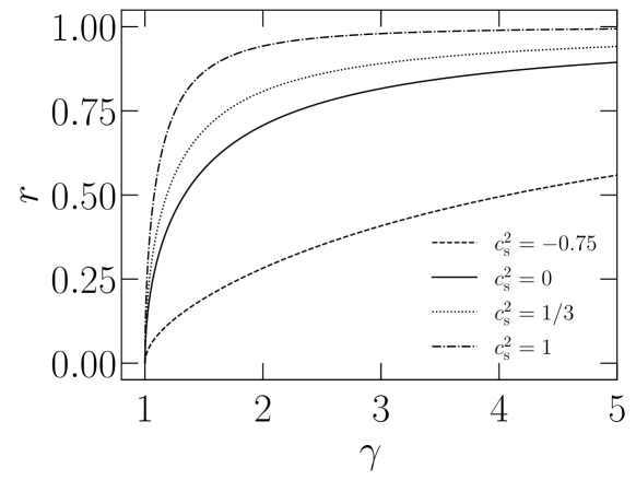
Figure 1: Ratio $r=\sqrt{\tilde{T}^{0i}\tilde{T}^{0i}}/\tilde{T}^{00}$ of a perfect fluid as a function of the Lorentz factor $\gamma$ for different values of $c_{\rm s}^{2}=\tilde{p}/\tilde{\rho}$.

The conservation form requires to express the primitive variables $\tilde{\rho}$ and $u^{i}$ in terms of the variables $\tilde{T}^{0\mu}$ to compute $\tilde{T}^{ij}$. Once that we have a closed form for the fluxes $\tilde{T}^{\mu j}$ and forces $\tilde{f}^{\mu}_{H}$ in terms of $\tilde{T}^{0\mu}$, we can solve the system in (1.2daaacahdeftvwacaeai). Assuming a generic but constant equation of state $c_{\rm s}^{2}=\tilde{p}/\tilde{\rho}$, we first compute the following variables,

$$\tilde{T}^{00}=(1+c_{\rm s}^{2})\,\tilde{\rho}\,\biggl{(}\gamma^{2}-\frac{c_{\rm s}^{2}}{1+c_{\rm s}^{2}}\biggr{)}\,,\qquad\tilde{T}^{0i}\tilde{T}^{0i}=(1+c_{\rm s}^{2})^{2}\tilde{\rho}^{2}\gamma^{4}u^{2}\,,$$ (1.2daaacahdeftvwacaeal)

and define the ratio

$$r^{2}=\frac{\tilde{T}^{0i}\tilde{T}^{0i}}{({\tilde{T}^{00}})^{2}}=\frac{\gamma^{4}u^{2}}{\Bigl{(}\gamma^{2}-\frac{c_{\rm s}^{2}}{1+c_{\rm s}^{2}}\Bigr{)}^{2}}=\frac{\gamma^{2}(\gamma^{2}-1)}{\Bigl{(}\gamma^{2}-\frac{c_{\rm s}^{2}}{1+c_{\rm s}^{2}}\Bigr{)}^{2}}\,,$$ (1.2daaacahdeftvwacaeam)

which is shown in figure 1 as a function of $\gamma$ for different values of $c_{\rm s}^{2}$. We note that for this relation to be valid we require $\delta=0$, as any rescaling of $u^{i}$ would affect the relation between $\gamma^{2}$ and $u^{2}$. This equation can be solved for $\gamma^{2}$,

$$\gamma^{2}=\frac{1}{2(1-r^{2})}\left[1-2r^{2}\frac{c_{\rm s}^{2}}{1+c_{\rm s}^{2}}+\sqrt{1-4r^{2}\frac{c_{\rm s}^{2}}{(1+c_{\rm s}^{2})^{2}}}\ \right]\,,$$ (1.2daaacahdeftvwacaean)

where we take the positive root of the quadratic equation to ensure $\gamma^{2}\geq 1$. The primitive variables can be expressed in terms of $\tilde{T}^{0\mu}$ and $\gamma^{2}$ as

$$\tilde{\rho}=\frac{\tilde{T}^{00}}{(1+c_{\rm s}^{2})\gamma^{2}-c_{\rm s}^{2}},\qquad u^{i}=\frac{\tilde{T}^{0i}}{(1+c_{\rm s}^{2})\tilde{\rho}\gamma^{2}}=\frac{\tilde{T}^{0i}}{\tilde{T}^{00}}\biggl{[}1-\frac{c_{\rm s}^{2}}{(1+c_{\rm s}^{2})\gamma^{2}}\biggr{]}\,,$$ (1.2daaacahdeftvwacaeao)

such that the flux $\tilde{T}^{ij}$ is

$$\tilde{T}^{ij}=\bigl{[}(1+c_{\rm s}^{2})\,\gamma^{2}u^{i}u^{j}+c_{\rm s}^{2}\delta^{ij}\bigr{]}\,\tilde{\rho}=\frac{\tilde{T}^{0i}\tilde{T}^{0j}}{(1+c_{\rm s}^{2})\tilde{\rho}\gamma^{2}}+c_{\rm s}^{2}\,\tilde{\rho}\,\delta^{ij}\,.$$ (1.2daaacahdeftvwacaeap)

Using this formalism, the non-linear relativistic system of equations can be solved evolving the $\tilde{T}^{0\mu}$ components and then the primitive fluid variables $\tilde{\rho}$ and $u^{i}$ can be reconstructed from $T^{0\mu}$.

Conservation form in the subrelativistic limit

In the subrelativistic limit, $\gamma^{2}\to 1$ and the components of the stress-energy tensor become

$$\tilde{T}^{00}=\tilde{\rho}\,,\qquad\tilde{T}^{0i}=(1+c_{\rm s}^{2})\,\tilde{\rho}u^{i}\,,\qquad\tilde{T}^{ij}=\frac{1}{1+c_{\rm s}^{2}}\frac{\tilde{T}^{0i}\tilde{T}^{0j}}{\tilde{T}^{00}}+c_{\rm s}^{2}\,\tilde{T}^{00}\,\delta^{ij}\,.$$ (1.2daaacahdeftvwacaeaq)

These relations are tempting due to their simplicity, as they already relate $\tilde{T}^{ij}$ with $\tilde{T}^{0\mu}$, allowing us to solve for the system in its conservation form. However, we have already pointed out that the term $\partial_{\tau}\gamma^{2}$ lead to additional terms in the energy conservation equation that are not negligible in the subrelativistic regime, as we will show explicitly in section 3.4. Therefore, when we set $\gamma\to 1$ to express $\tilde{T}^{ij}$ in terms of $\tilde{T}^{0\mu}$, we are indirectly setting $\partial_{\tau}\gamma^{2}\to 0$ and hence, ignoring potentially relevant terms. To recover these terms, let us approximate (1.2daaacahdeftvwacaean) up to first order in $r^{2}\equiv\tilde{T}^{0i}\,\tilde{T}^{0i}/(\tilde{T}^{00})^{2}$,

$$\gamma^{2}=1+\frac{r^{2}}{(1+c_{\rm s}^{2})^{2}}+{\cal O}(r^{4})\,.$$ (1.2daaacahdeftvwacaear)

The $r^{2}\to 0$ limit is equivalent to the subrelativistic limit, as can be seen in figure 1. Then, substituting $\gamma^{2}$ up to first order in $r^{2}$ into $\tilde{T}^{0\mu}$, we find

$$\tilde{T}^{00}=\biggl{(}1+\frac{r^{2}}{1+c_{\rm s}^{2}}\biggr{)}\tilde{\rho}\,,\qquad\tilde{T}^{0i}=\biggl{(}1+c_{\rm s}^{2}+\frac{r^{2}}{1+c_{\rm s}^{2}}\biggr{)}\tilde{\rho}\,u^{i}\,,$$ (1.2daaacahdeftvwacaeas)

which allows us to express $\tilde{T}^{ij}$ up to first order in $r^{2}$,

$$\tilde{T}^{ij}=\frac{1}{1+c_{\rm s}^{2}}\frac{\tilde{T}^{0i}\tilde{T}^{0j}}{\tilde{T}^{00}}\biggl{(}1+\frac{r^{2}c_{\rm s}^{2}}{1+c_{\rm s}^{2}}\biggr{)}+c_{\rm s}^{2}\tilde{T}^{00}\biggl{(}1-\frac{r^{2}}{1+c_{\rm s}^{2}}\biggr{)}\,\delta^{ij}+{\cal O}(r^{4})\,.$$ (1.2daaacahdeftvwacaeat)

This relation includes the next-to-leading-order term in $r^{2}$. Hence, it takes into account the corresponding corrections in $\tilde{T}^{0\mu}$ and leads to the correct subrelativistic limit.

To show this, let us expand the conservation laws of (1.2daaacahdeftvwacaeai) for conformal time in terms of $\tilde{\rho}$ and $\textstyle u$, as we will do for the full relativistic system in section 3.4.2, to find the non-conservation form of the equations,

$$\partial_{\tau}\tilde{\rho}+\frac{\tilde{\rho}}{1+c_{\rm s}^{2}}\partial_{\tau}r^{2}+(1+c_{\rm s}^{2})\,\partial_{i}(\tilde{\rho}u^{i})=\tilde{f}_{H}^{0}\,,$$ (1.2daaacahdeftvwacaeaua)

$$u^{i}\,\partial_{\tau}\tilde{\rho}+\tilde{\rho}\,\partial_{\tau}u^{i}+\frac{\tilde{\rho}u^{i}}{(1+c_{\rm s}^{2})^{2}}\partial_{\tau}r^{2}+\,\partial_{j}\bigl{(}\tilde{\rho}u^{i}u^{j}\bigr{)}+\frac{c_{\rm s}^{2}}{1+c_{\rm s}^{2}}\partial_{i}\tilde{\rho}=\frac{\tilde{f}_{H}^{i}}{1+c_{\rm s}^{2}}\,.$$ (1.2daaacahdeftvwacaeaub)

Note that the next-to-leading-order term is proportional to $\partial_{\tau}r^{2}$, which can be expressed as

$$\partial_{\tau}r^{2}=(1+c_{\rm s}^{2})^{2}\partial_{\tau}\gamma^{2}=(1+c_{\rm s}^{2})^{2}\gamma^{2}\partial_{\tau}u^{2}=(1+c_{\rm s}^{2})^{2}\,\partial_{\tau}u^{2}+{\cal O}(r^{4})\,.$$ (1.2daaacahdeftvwacaeauav)

Therefore, taking the product of $u^{i}$ with the momentum equation, and keeping only leading-order terms, we find

$${\textstyle{1\over 2}}\tilde{\rho}\,\partial_{\tau}u^{2}=-\frac{c_{\rm s}^{2}}{1+c_{\rm s}^{2}}u^{i}\partial_{i}\tilde{\rho}+\frac{u^{i}f_{H}^{i}}{1+c_{\rm s}^{2}}\,,$$ (1.2daaacahdeftvwacaeauaw)

where the right-hand side corresponds to the work done by the pressure gradient, $c_{\rm s}^{2}\,\mathchoice{\mbox{\boldmath$\displaystyle u$}}{\mbox{\boldmath$\textstyle u$}}{\mbox{\boldmath$\scriptstyle u$}}{\mbox{\boldmath$\scriptscriptstyle u$}}{}\cdot\mathchoice{\mbox{\boldmath$\displaystyle\nabla$}}{\mbox{\boldmath$\textstyle\nabla$}}{\mbox{\boldmath$\scriptstyle\nabla$}}{\mbox{\boldmath$\scriptscriptstyle\nabla$}}{}\tilde{\rho}$, and external forces, $\mathchoice{\mbox{\boldmath$\displaystyle u$}}{\mbox{\boldmath$\textstyle u$}}{\mbox{\boldmath$\scriptstyle u$}}{\mbox{\boldmath$\scriptscriptstyle u$}}{}\cdot\mathchoice{\mbox{\boldmath$\displaystyle\tilde{f}$}}{\mbox{\boldmath$\textstyle\tilde{f}$}}{\mbox{\boldmath$\scriptstyle\tilde{f}$}}{\mbox{\boldmath$\scriptscriptstyle\tilde{f}$}}{}_{H}$. As expected for perfect fluids, the work done by these forces is a reversible process and, hence, they do not produce entropy [68].

Equation (1.2daaacahdeftvwacaeauaw) shows that neglecting the next-to-leading order term $r^{2}$ in the stress-energy tensor components in (1.2daaacahdeftvwacaeas) is equivalent to ignoring terms that are non-negligible in the subrelativistic limit. Substituting this term back in the energy and momentum conservation equations, we find

$$\partial_{\tau}\ln\tilde{\rho}=-(1+c_{\rm s}^{2})\,\mathchoice{\mbox{\boldmath$\displaystyle\nabla$}}{\mbox{\boldmath$\textstyle\nabla$}}{\mbox{\boldmath$\scriptstyle\nabla$}}{\mbox{\boldmath$\scriptscriptstyle\nabla$}}{}\cdot\mathchoice{\mbox{\boldmath$\displaystyle u$}}{\mbox{\boldmath$\textstyle u$}}{\mbox{\boldmath$\scriptstyle u$}}{\mbox{\boldmath$\scriptscriptstyle u$}}{}-(1-c_{\rm s}^{2})\,(\mathchoice{\mbox{\boldmath$\displaystyle u$}}{\mbox{\boldmath$\textstyle u$}}{\mbox{\boldmath$\scriptstyle u$}}{\mbox{\boldmath$\scriptscriptstyle u$}}{}\cdot\mathchoice{\mbox{\boldmath$\displaystyle\nabla$}}{\mbox{\boldmath$\textstyle\nabla$}}{\mbox{\boldmath$\scriptstyle\nabla$}}{\mbox{\boldmath$\scriptscriptstyle\nabla$}}{})\ln\tilde{\rho}+\frac{\tilde{f}_{H}^{0}}{\tilde{\rho}}-2\,\frac{\mathchoice{\mbox{\boldmath$\displaystyle u$}}{\mbox{\boldmath$\textstyle u$}}{\mbox{\boldmath$\scriptstyle u$}}{\mbox{\boldmath$\scriptscriptstyle u$}}{}\cdot\mathchoice{\mbox{\boldmath$\displaystyle\tilde{f}$}}{\mbox{\boldmath$\textstyle\tilde{f}$}}{\mbox{\boldmath$\scriptstyle\tilde{f}$}}{\mbox{\boldmath$\scriptscriptstyle\tilde{f}$}}{}_{H}}{\tilde{\rho}}\,,$$ (1.2daaacahdeftvwacaeauaxa)

$$\partial_{\tau}\mathchoice{\mbox{\boldmath$\displaystyle u$}}{\mbox{\boldmath$\textstyle u$}}{\mbox{\boldmath$\scriptstyle u$}}{\mbox{\boldmath$\scriptscriptstyle u$}}{}+(\mathchoice{\mbox{\boldmath$\displaystyle u$}}{\mbox{\boldmath$\textstyle u$}}{\mbox{\boldmath$\scriptstyle u$}}{\mbox{\boldmath$\scriptscriptstyle u$}}{}\cdot\mathchoice{\mbox{\boldmath$\displaystyle\nabla$}}{\mbox{\boldmath$\textstyle\nabla$}}{\mbox{\boldmath$\scriptstyle\nabla$}}{\mbox{\boldmath$\scriptscriptstyle\nabla$}}{})\mathchoice{\mbox{\boldmath$\displaystyle u$}}{\mbox{\boldmath$\textstyle u$}}{\mbox{\boldmath$\scriptstyle u$}}{\mbox{\boldmath$\scriptscriptstyle u$}}{}=\mathchoice{\mbox{\boldmath$\displaystyle u$}}{\mbox{\boldmath$\textstyle u$}}{\mbox{\boldmath$\scriptstyle u$}}{\mbox{\boldmath$\scriptscriptstyle u$}}{}\biggl{[}c_{\rm s}^{2}\mathchoice{\mbox{\boldmath$\displaystyle\nabla$}}{\mbox{\boldmath$\textstyle\nabla$}}{\mbox{\boldmath$\scriptstyle\nabla$}}{\mbox{\boldmath$\scriptscriptstyle\nabla$}}{}\cdot\mathchoice{\mbox{\boldmath$\displaystyle u$}}{\mbox{\boldmath$\textstyle u$}}{\mbox{\boldmath$\scriptstyle u$}}{\mbox{\boldmath$\scriptscriptstyle u$}}{}+c_{\rm s}^{2}\,\frac{1-c_{\rm s}^{2}}{1+c_{\rm s}^{2}}\,(\mathchoice{\mbox{\boldmath$\displaystyle u$}}{\mbox{\boldmath$\textstyle u$}}{\mbox{\boldmath$\scriptstyle u$}}{\mbox{\boldmath$\scriptscriptstyle u$}}{}\cdot\mathchoice{\mbox{\boldmath$\displaystyle\nabla$}}{\mbox{\boldmath$\textstyle\nabla$}}{\mbox{\boldmath$\scriptstyle\nabla$}}{\mbox{\boldmath$\scriptscriptstyle\nabla$}}{})\ln\tilde{\rho}-\frac{\tilde{f}_{H}^{0}}{\tilde{\rho}}+\frac{2c_{\rm s}^{2}}{(1+c_{\rm s}^{2})\tilde{\rho}}\,\mathchoice{\mbox{\boldmath$\displaystyle u$}}{\mbox{\boldmath$\textstyle u$}}{\mbox{\boldmath$\scriptstyle u$}}{\mbox{\boldmath$\scriptscriptstyle u$}}{}\cdot\mathchoice{\mbox{\boldmath$\displaystyle\tilde{f}$}}{\mbox{\boldmath$\textstyle\tilde{f}$}}{\mbox{\boldmath$\scriptstyle\tilde{f}$}}{\mbox{\boldmath$\scriptscriptstyle\tilde{f}$}}{}_{H}\biggr{]}$$

$$-\frac{c_{\rm s}^{2}}{1+c_{\rm s}^{2}}\mathchoice{\mbox{\boldmath$\displaystyle\nabla$}}{\mbox{\boldmath$\textstyle\nabla$}}{\mbox{\boldmath$\scriptstyle\nabla$}}{\mbox{\boldmath$\scriptscriptstyle\nabla$}}{}\ln\tilde{\rho}+\frac{\mathchoice{\mbox{\boldmath$\displaystyle\tilde{f}$}}{\mbox{\boldmath$\textstyle\tilde{f}$}}{\mbox{\boldmath$\scriptstyle\tilde{f}$}}{\mbox{\boldmath$\scriptscriptstyle\tilde{f}$}}{}_{H}}{(1+c_{\rm s}^{2})\tilde{\rho}}\,.$$ (1.2daaacahdeftvwacaeauaxb)

This set of equations is equivalent to the one presented in the introduction; see (1.2da) and (1.2db), in the absence of external forces. They generalize the set of equations used in previous work to values of the speed of sound different than $c_{\rm s}^{2}=1/3$ but still relativistic, i.e., $c_{\rm s}^{2}\sim{\cal O}(1)$, introducing terms that break conformal invariance. These equations also include corrections to the energy (also pointed out in [58]; see footnote 3), and to the momentum equations with respect to previous work. These equations are in a non-conservation form as they are not explicitly written in the form of (1.2daaacahdeftvwacaeak). In the next section, we compute the relativistic version of the conservation laws in the non-conservation form, explicitly corresponding to equations for the primitive variables $\tilde{\rho}$ and $\textstyle u$.

3.4 Non-conservation form of relativistic hydrodynamics

The non-conservation form is obtained expressing explicitly the stress-energy components in terms of the primitive variables, $\tilde{\rho}$ and $\textstyle u$. In the following, the extension of the system of equations given in (1.2daaacahdeftvwacaeauaxa) and (1.2daaacahdeftvwacaeauaxb) to the fully relativistic regime is done, up to our knowledge, for the first time for a perfect fluid in an expanding background. For compactness, we set $\alpha=1$ and $\delta=0$ in the following, but the equations can be generalized to any rescaling choice.

3.4.1 Relativistic equations

Energy equation

Let us start with the equation of energy conservation taking (1.2daaacahdeftvwacaeai) for $\mu=0$,

$$\partial_{\tau}\bigl{[}(\tilde{p}+\tilde{\rho})\gamma^{2}-\tilde{p}\bigr{]}+\partial_{i}\bigl{[}(\tilde{p}+\tilde{\rho})\gamma^{2}u^{i}\bigr{]}=\tilde{f}_{H}^{0}\,.$$ (1.2daaacahdeftvwacaeauaxay)

We divide the equation by $(\tilde{p}+\tilde{\rho})\gamma^{2}$,

$$\partial_{\tau}\ln\bigl{[}(\tilde{p}+\tilde{\rho})\gamma^{2}\bigr{]}-\frac{\partial_{\tau}\tilde{p}}{(\tilde{p}+\tilde{\rho})\gamma^{2}}+u^{i}\partial_{i}\ln\bigl{[}(\tilde{p}+\tilde{\rho})\gamma^{2}\bigr{]}+\partial_{i}u^{i}=\frac{\tilde{f}_{H}^{0}}{(\tilde{p}+\tilde{\rho})\gamma^{2}}\,.$$ (1.2daaacahdeftvwacaeauaxaz)

In terms of a constant speed of sound $\tilde{p}=c_{\rm s}^{2}\tilde{\rho}$, we find

$$\biggl{[}1-\frac{c_{\rm s}^{2}}{(1+c_{\rm s}^{2})\gamma^{2}}\biggr{]}\partial_{\tau}\ln\tilde{\rho} \,+\partial_{\tau}\ln\gamma^{2}=-\mathchoice{\mbox{\boldmath$\displaystyle\nabla$}}{\mbox{\boldmath$\textstyle\nabla$}}{\mbox{\boldmath$\scriptstyle\nabla$}}{\mbox{\boldmath$\scriptscriptstyle\nabla$}}{}\cdot\mathchoice{\mbox{\boldmath$\displaystyle u$}}{\mbox{\boldmath$\textstyle u$}}{\mbox{\boldmath$\scriptstyle u$}}{\mbox{\boldmath$\scriptscriptstyle u$}}{}-(\mathchoice{\mbox{\boldmath$\displaystyle u$}}{\mbox{\boldmath$\textstyle u$}}{\mbox{\boldmath$\scriptstyle u$}}{\mbox{\boldmath$\scriptscriptstyle u$}}{}\cdot\mathchoice{\mbox{\boldmath$\displaystyle\nabla$}}{\mbox{\boldmath$\textstyle\nabla$}}{\mbox{\boldmath$\scriptstyle\nabla$}}{\mbox{\boldmath$\scriptscriptstyle\nabla$}}{})\ln(\tilde{\rho}\gamma^{2})+\frac{\tilde{f}_{H}^{0}}{(1+c_{\rm s}^{2})\tilde{\rho}\gamma^{2}}\,.$$ (1.2daaacahdeftvwacaeauaxba)

We can express the coefficient of $\partial_{\tau}\ln\tilde{\rho}$ as $(1+c_{\rm s}^{2}u^{2})/(1+c_{\rm s}^{2})$. Hence,

$$\partial_{\tau}\ln\tilde{\rho}\,+\frac{1+c_{\rm s}^{2}}{1+c_{\rm s}^{2}u^{2}}\partial_{\tau}\ln\gamma^{2}$$

$$=-\frac{1+c_{\rm s}^{2}}{1+c_{\rm s}^{2}u^{2}}\bigl{[}\mathchoice{\mbox{\boldmath$\displaystyle\nabla$}}{\mbox{\boldmath$\textstyle\nabla$}}{\mbox{\boldmath$\scriptstyle\nabla$}}{\mbox{\boldmath$\scriptscriptstyle\nabla$}}{}\cdot\mathchoice{\mbox{\boldmath$\displaystyle u$}}{\mbox{\boldmath$\textstyle u$}}{\mbox{\boldmath$\scriptstyle u$}}{\mbox{\boldmath$\scriptscriptstyle u$}}{}+\bigl{(}\mathchoice{\mbox{\boldmath$\displaystyle u$}}{\mbox{\boldmath$\textstyle u$}}{\mbox{\boldmath$\scriptstyle u$}}{\mbox{\boldmath$\scriptscriptstyle u$}}{}\cdot\mathchoice{\mbox{\boldmath$\displaystyle\nabla$}}{\mbox{\boldmath$\textstyle\nabla$}}{\mbox{\boldmath$\scriptstyle\nabla$}}{\mbox{\boldmath$\scriptscriptstyle\nabla$}}{}\bigr{)}\ln(\tilde{\rho}\gamma^{2})\bigr{]}+\frac{\tilde{f}_{H}^{0}}{(1+c_{\rm s}^{2}u^{2})\tilde{\rho}\gamma^{2}}\,.$$ (1.2daaacahdeftvwacaeauaxbb)

As mentioned above, previous work considered this expression directly taking the subrelativistic limit $\gamma\simeq 1$ for $c_{\rm s}^{2}=1/3$ and $\beta=4$, such that $\tilde{f}_{H}^{0}=0$ (see, e.g., [10, 25, 32]). However, as shown in previous section, $\partial_{\tau}\gamma^{2}$ cannot be neglected in the subrelativistic regime. In the following, we will keep all relativistic terms to find the relativistic conservation laws. Then, to double check the equations found in the previous section [see (1.2daaacahdeftvwacaeauaxa) and (1.2daaacahdeftvwacaeauaxb)] we will take the subrelativistic limit directly from the relativistic equations expressed in their non-conservation form.

Momentum equation

We now proceed to compute the momentum equation, given by the spatial components of (1.2daaacahdeftvwacaeai),

$$\partial_{\tau}\tilde{T}^{0i}+\partial_{j}\tilde{T}^{ij}=\partial_{\tau}\bigl{[}(\tilde{p}+\tilde{\rho})\gamma^{2}u^{i}\bigr{]}+\partial_{j}\bigl{[}(\tilde{p}+\tilde{\rho})\gamma^{2}u^{i}u^{j}+\tilde{p}\delta^{ij}\bigr{]}=\tilde{f}_{H}^{i}\,,$$ (1.2daaacahdeftvwacaeauaxbc)

where we note that $\tilde{f}_{H}^{i}=0$ when $\beta=4$, but we keep it for generality. We then divide by $(\tilde{p}+\tilde{\rho})\gamma^{2}$ and find

$$\partial_{\tau}u^{i}+u^{i}\partial_{\tau}\ln\bigl{[}(\tilde{p}+\tilde{\rho})\gamma^{2}\bigr{]}+\partial_{j}(u^{i}u^{j})+u^{i}u^{j}\partial_{j}\ln\bigl{[}(\tilde{p}+\tilde{\rho})\gamma^{2}\bigr{]}+\frac{\partial_{i}\tilde{p}}{(\tilde{p}+\tilde{\rho})\gamma^{2}}=\frac{\tilde{f}_{H}^{i}}{(\tilde{p}+\tilde{\rho})\gamma^{2}}\,.$$ (1.2daaacahdeftvwacaeauaxbd)

We now again use a generic constant equation of state $\tilde{p}=c_{\rm s}^{2}\tilde{\rho}$,

$$\partial_{\tau}\mathchoice{\mbox{\boldmath$\displaystyle u$}}{\mbox{\boldmath$\textstyle u$}}{\mbox{\boldmath$\scriptstyle u$}}{\mbox{\boldmath$\scriptscriptstyle u$}}{}+(\mathchoice{\mbox{\boldmath$\displaystyle u$}}{\mbox{\boldmath$\textstyle u$}}{\mbox{\boldmath$\scriptstyle u$}}{\mbox{\boldmath$\scriptscriptstyle u$}}{}\cdot\mathchoice{\mbox{\boldmath$\displaystyle\nabla$}}{\mbox{\boldmath$\textstyle\nabla$}}{\mbox{\boldmath$\scriptstyle\nabla$}}{\mbox{\boldmath$\scriptscriptstyle\nabla$}}{})\,\mathchoice{\mbox{\boldmath$\displaystyle u$}}{\mbox{\boldmath$\textstyle u$}}{\mbox{\boldmath$\scriptstyle u$}}{\mbox{\boldmath$\scriptscriptstyle u$}}{}+\mathchoice{\mbox{\boldmath$\displaystyle u$}}{\mbox{\boldmath$\textstyle u$}}{\mbox{\boldmath$\scriptstyle u$}}{\mbox{\boldmath$\scriptscriptstyle u$}}{}\bigl{[}\partial_{\tau}\ln\tilde{\rho}\,+\partial_{\tau}\ln\gamma^{2}+\mathchoice{\mbox{\boldmath$\displaystyle\nabla$}}{\mbox{\boldmath$\textstyle\nabla$}}{\mbox{\boldmath$\scriptstyle\nabla$}}{\mbox{\boldmath$\scriptscriptstyle\nabla$}}{}\cdot\mathchoice{\mbox{\boldmath$\displaystyle u$}}{\mbox{\boldmath$\textstyle u$}}{\mbox{\boldmath$\scriptstyle u$}}{\mbox{\boldmath$\scriptscriptstyle u$}}{}+\bigl{(}\mathchoice{\mbox{\boldmath$\displaystyle u$}}{\mbox{\boldmath$\textstyle u$}}{\mbox{\boldmath$\scriptstyle u$}}{\mbox{\boldmath$\scriptscriptstyle u$}}{}\cdot\mathchoice{\mbox{\boldmath$\displaystyle\nabla$}}{\mbox{\boldmath$\textstyle\nabla$}}{\mbox{\boldmath$\scriptstyle\nabla$}}{\mbox{\boldmath$\scriptscriptstyle\nabla$}}{}\bigr{)}\ln\bigl{(}\tilde{\rho}\gamma^{2}\bigr{)}\bigr{]}$$

$$=-\frac{c_{\rm s}^{2}}{(1+c_{\rm s}^{2})\gamma^{2}}\mathchoice{\mbox{\boldmath$\displaystyle\nabla$}}{\mbox{\boldmath$\textstyle\nabla$}}{\mbox{\boldmath$\scriptstyle\nabla$}}{\mbox{\boldmath$\scriptscriptstyle\nabla$}}{}\ln\tilde{\rho}+\frac{1}{1+c_{\rm s}^{2}}\frac{\mathchoice{\mbox{\boldmath$\displaystyle\tilde{f}$}}{\mbox{\boldmath$\textstyle\tilde{f}$}}{\mbox{\boldmath$\scriptstyle\tilde{f}$}}{\mbox{\boldmath$\scriptscriptstyle\tilde{f}$}}{}_{H}}{\tilde{\rho}\gamma^{2}}\,.$$ (1.2daaacahdeftvwacaeauaxbe)

Again, we note that previous work have considered the subrelativistic limit of this equation using $\gamma\simeq 1$ for $\beta=4$ such that $\tilde{f}_{H}^{i}=0$ (see, e.g., [10, 25, 32]). Similar as for the energy equation, the subrelativistic term contained in $\partial_{\tau}\gamma^{2}$ will also enter the momentum equation.

We can now use the energy equation [see (1.2daaacahdeftvwacaeauaxbb)] to get rid of $\partial_{\tau}\ln\tilde{\rho}$ in the relativistic momentum conservation,

$$\partial_{\tau}\mathchoice{\mbox{\boldmath$\displaystyle u$}}{\mbox{\boldmath$\textstyle u$}}{\mbox{\boldmath$\scriptstyle u$}}{\mbox{\boldmath$\scriptscriptstyle u$}}{}+(\mathchoice{\mbox{\boldmath$\displaystyle u$}}{\mbox{\boldmath$\textstyle u$}}{\mbox{\boldmath$\scriptstyle u$}}{\mbox{\boldmath$\scriptscriptstyle u$}}{}\cdot\mathchoice{\mbox{\boldmath$\displaystyle\nabla$}}{\mbox{\boldmath$\textstyle\nabla$}}{\mbox{\boldmath$\scriptstyle\nabla$}}{\mbox{\boldmath$\scriptscriptstyle\nabla$}}{})\,\mathchoice{\mbox{\boldmath$\displaystyle u$}}{\mbox{\boldmath$\textstyle u$}}{\mbox{\boldmath$\scriptstyle u$}}{\mbox{\boldmath$\scriptscriptstyle u$}}{}=\frac{\mathchoice{\mbox{\boldmath$\displaystyle u$}}{\mbox{\boldmath$\textstyle u$}}{\mbox{\boldmath$\scriptstyle u$}}{\mbox{\boldmath$\scriptscriptstyle u$}}{}}{(1+c_{\rm s}^{2}u^{2})\gamma^{2}}\biggl{[}c_{\rm s}^{2}\partial_{\tau}\ln\gamma^{2}+c_{\rm s}^{2}\mathchoice{\mbox{\boldmath$\displaystyle\nabla$}}{\mbox{\boldmath$\textstyle\nabla$}}{\mbox{\boldmath$\scriptstyle\nabla$}}{\mbox{\boldmath$\scriptscriptstyle\nabla$}}{}\cdot\mathchoice{\mbox{\boldmath$\displaystyle u$}}{\mbox{\boldmath$\textstyle u$}}{\mbox{\boldmath$\scriptstyle u$}}{\mbox{\boldmath$\scriptscriptstyle u$}}{}+c_{\rm s}^{2}\,\bigl{(}\mathchoice{\mbox{\boldmath$\displaystyle u$}}{\mbox{\boldmath$\textstyle u$}}{\mbox{\boldmath$\scriptstyle u$}}{\mbox{\boldmath$\scriptscriptstyle u$}}{}\cdot\mathchoice{\mbox{\boldmath$\displaystyle\nabla$}}{\mbox{\boldmath$\textstyle\nabla$}}{\mbox{\boldmath$\scriptstyle\nabla$}}{\mbox{\boldmath$\scriptscriptstyle\nabla$}}{}\bigr{)}\ln\bigl{(}\tilde{\rho}\gamma^{2}\bigr{)}-\frac{\tilde{f}_{H}^{0}}{\tilde{\rho}}\biggr{]}$$

$$-\frac{c_{\rm s}^{2}}{(1+c_{\rm s}^{2})\gamma^{2}}\mathchoice{\mbox{\boldmath$\displaystyle\nabla$}}{\mbox{\boldmath$\textstyle\nabla$}}{\mbox{\boldmath$\scriptstyle\nabla$}}{\mbox{\boldmath$\scriptscriptstyle\nabla$}}{}\ln\tilde{\rho}+\frac{1}{1+c_{\rm s}^{2}}\frac{\mathchoice{\mbox{\boldmath$\displaystyle\tilde{f}$}}{\mbox{\boldmath$\textstyle\tilde{f}$}}{\mbox{\boldmath$\scriptstyle\tilde{f}$}}{\mbox{\boldmath$\scriptscriptstyle\tilde{f}$}}{}_{H}}{\tilde{\rho}\gamma^{2}}\,.$$ (1.2daaacahdeftvwacaeauaxbf)

Evolution of the Lorentz factor

In order to get rid of the $\partial_{\tau}\ln\gamma^{2}$ term that appears in both the energy and momentum equations, an evolution equation for the Lorentz factor can be computed from the momentum equation, by contracting it with the velocity field $\textstyle u$,

$$\partial_{\tau}\ln\gamma^{2}=\gamma^{2}\partial_{\tau}u^{2}=2\gamma^{2}\mathchoice{\mbox{\boldmath$\displaystyle u$}}{\mbox{\boldmath$\textstyle u$}}{\mbox{\boldmath$\scriptstyle u$}}{\mbox{\boldmath$\scriptscriptstyle u$}}{}\cdot\partial_{\tau}\mathchoice{\mbox{\boldmath$\displaystyle u$}}{\mbox{\boldmath$\textstyle u$}}{\mbox{\boldmath$\scriptstyle u$}}{\mbox{\boldmath$\scriptscriptstyle u$}}{}$$

$$=\frac{2u^{2}}{1+c_{\rm s}^{2}u^{2}}\biggl{[}c_{\rm s}^{2}\,\partial_{\tau}\ln\gamma^{2}+c_{\rm s}^{2}\,\mathchoice{\mbox{\boldmath$\displaystyle\nabla$}}{\mbox{\boldmath$\textstyle\nabla$}}{\mbox{\boldmath$\scriptstyle\nabla$}}{\mbox{\boldmath$\scriptscriptstyle\nabla$}}{}\cdot\mathchoice{\mbox{\boldmath$\displaystyle u$}}{\mbox{\boldmath$\textstyle u$}}{\mbox{\boldmath$\scriptstyle u$}}{\mbox{\boldmath$\scriptscriptstyle u$}}{}+c_{\rm s}^{2}\,\bigl{(}\mathchoice{\mbox{\boldmath$\displaystyle u$}}{\mbox{\boldmath$\textstyle u$}}{\mbox{\boldmath$\scriptstyle u$}}{\mbox{\boldmath$\scriptscriptstyle u$}}{}\cdot\mathchoice{\mbox{\boldmath$\displaystyle\nabla$}}{\mbox{\boldmath$\textstyle\nabla$}}{\mbox{\boldmath$\scriptstyle\nabla$}}{\mbox{\boldmath$\scriptscriptstyle\nabla$}}{}\bigr{)}\ln(\tilde{\rho}\gamma^{2})-\frac{\tilde{f}_{H}^{0}}{\tilde{\rho}}\biggr{]}$$

$$-2\gamma^{2}\,\mathchoice{\mbox{\boldmath$\displaystyle u$}}{\mbox{\boldmath$\textstyle u$}}{\mbox{\boldmath$\scriptstyle u$}}{\mbox{\boldmath$\scriptscriptstyle u$}}{}\cdot(\mathchoice{\mbox{\boldmath$\displaystyle u$}}{\mbox{\boldmath$\textstyle u$}}{\mbox{\boldmath$\scriptstyle u$}}{\mbox{\boldmath$\scriptscriptstyle u$}}{}\cdot\mathchoice{\mbox{\boldmath$\displaystyle\nabla$}}{\mbox{\boldmath$\textstyle\nabla$}}{\mbox{\boldmath$\scriptstyle\nabla$}}{\mbox{\boldmath$\scriptscriptstyle\nabla$}}{})\mathchoice{\mbox{\boldmath$\displaystyle u$}}{\mbox{\boldmath$\textstyle u$}}{\mbox{\boldmath$\scriptstyle u$}}{\mbox{\boldmath$\scriptscriptstyle u$}}{}-\frac{2c_{\rm s}^{2}}{1+c_{\rm s}^{2}}(\mathchoice{\mbox{\boldmath$\displaystyle u$}}{\mbox{\boldmath$\textstyle u$}}{\mbox{\boldmath$\scriptstyle u$}}{\mbox{\boldmath$\scriptscriptstyle u$}}{}\cdot\mathchoice{\mbox{\boldmath$\displaystyle\nabla$}}{\mbox{\boldmath$\textstyle\nabla$}}{\mbox{\boldmath$\scriptstyle\nabla$}}{\mbox{\boldmath$\scriptscriptstyle\nabla$}}{})\ln\tilde{\rho}+\frac{2}{1+c_{\rm s}^{2}}\frac{\mathchoice{\mbox{\boldmath$\displaystyle u$}}{\mbox{\boldmath$\textstyle u$}}{\mbox{\boldmath$\scriptstyle u$}}{\mbox{\boldmath$\scriptscriptstyle u$}}{}\cdot\mathchoice{\mbox{\boldmath$\displaystyle\tilde{f}$}}{\mbox{\boldmath$\textstyle\tilde{f}$}}{\mbox{\boldmath$\scriptstyle\tilde{f}$}}{\mbox{\boldmath$\scriptscriptstyle\tilde{f}$}}{}_{H}}{\tilde{\rho}}\,.$$ (1.2daaacahdeftvwacaeauaxbg)

To simplify the computation, we first note that $\mathchoice{\mbox{\boldmath$\displaystyle\nabla$}}{\mbox{\boldmath$\textstyle\nabla$}}{\mbox{\boldmath$\scriptstyle\nabla$}}{\mbox{\boldmath$\scriptscriptstyle\nabla$}}{}\ln(\tilde{\rho}\gamma^{2})=\mathchoice{\mbox{\boldmath$\displaystyle\nabla$}}{\mbox{\boldmath$\textstyle\nabla$}}{\mbox{\boldmath$\scriptstyle\nabla$}}{\mbox{\boldmath$\scriptscriptstyle\nabla$}}{}\ln\tilde{\rho}+\mathchoice{\mbox{\boldmath$\displaystyle\nabla$}}{\mbox{\boldmath$\textstyle\nabla$}}{\mbox{\boldmath$\scriptstyle\nabla$}}{\mbox{\boldmath$\scriptscriptstyle\nabla$}}{}\ln\gamma^{2}$, such that

$$(\mathchoice{\mbox{\boldmath$\displaystyle u$}}{\mbox{\boldmath$\textstyle u$}}{\mbox{\boldmath$\scriptstyle u$}}{\mbox{\boldmath$\scriptscriptstyle u$}}{}\cdot\mathchoice{\mbox{\boldmath$\displaystyle\nabla$}}{\mbox{\boldmath$\textstyle\nabla$}}{\mbox{\boldmath$\scriptstyle\nabla$}}{\mbox{\boldmath$\scriptscriptstyle\nabla$}}{})\ln(\tilde{\rho}\gamma^{2})=(\mathchoice{\mbox{\boldmath$\displaystyle u$}}{\mbox{\boldmath$\textstyle u$}}{\mbox{\boldmath$\scriptstyle u$}}{\mbox{\boldmath$\scriptscriptstyle u$}}{}\cdot\mathchoice{\mbox{\boldmath$\displaystyle\nabla$}}{\mbox{\boldmath$\textstyle\nabla$}}{\mbox{\boldmath$\scriptstyle\nabla$}}{\mbox{\boldmath$\scriptscriptstyle\nabla$}}{})\ln\tilde{\rho}+(\mathchoice{\mbox{\boldmath$\displaystyle u$}}{\mbox{\boldmath$\textstyle u$}}{\mbox{\boldmath$\scriptstyle u$}}{\mbox{\boldmath$\scriptscriptstyle u$}}{}\cdot\mathchoice{\mbox{\boldmath$\displaystyle\nabla$}}{\mbox{\boldmath$\textstyle\nabla$}}{\mbox{\boldmath$\scriptstyle\nabla$}}{\mbox{\boldmath$\scriptscriptstyle\nabla$}}{})\ln\gamma^{2}=(\mathchoice{\mbox{\boldmath$\displaystyle u$}}{\mbox{\boldmath$\textstyle u$}}{\mbox{\boldmath$\scriptstyle u$}}{\mbox{\boldmath$\scriptscriptstyle u$}}{}\cdot\mathchoice{\mbox{\boldmath$\displaystyle\nabla$}}{\mbox{\boldmath$\textstyle\nabla$}}{\mbox{\boldmath$\scriptstyle\nabla$}}{\mbox{\boldmath$\scriptscriptstyle\nabla$}}{})\ln\tilde{\rho}+2\gamma^{2}\,\mathchoice{\mbox{\boldmath$\displaystyle u$}}{\mbox{\boldmath$\textstyle u$}}{\mbox{\boldmath$\scriptstyle u$}}{\mbox{\boldmath$\scriptscriptstyle u$}}{}\cdot(\mathchoice{\mbox{\boldmath$\displaystyle u$}}{\mbox{\boldmath$\textstyle u$}}{\mbox{\boldmath$\scriptstyle u$}}{\mbox{\boldmath$\scriptscriptstyle u$}}{}\cdot\mathchoice{\mbox{\boldmath$\displaystyle\nabla$}}{\mbox{\boldmath$\textstyle\nabla$}}{\mbox{\boldmath$\scriptstyle\nabla$}}{\mbox{\boldmath$\scriptscriptstyle\nabla$}}{})\mathchoice{\mbox{\boldmath$\displaystyle u$}}{\mbox{\boldmath$\textstyle u$}}{\mbox{\boldmath$\scriptstyle u$}}{\mbox{\boldmath$\scriptscriptstyle u$}}{}\,.$$ (1.2daaacahdeftvwacaeauaxbh)

Hence, we finally find

$${\textstyle{1\over 2}}\partial_{\tau}\ln\gamma^{2}=\frac{1}{1-c_{\rm s}^{2}u^{2}}\biggl{[}u^{2}\biggl{(}c_{\rm s}^{2}\,\mathchoice{\mbox{\boldmath$\displaystyle\nabla$}}{\mbox{\boldmath$\textstyle\nabla$}}{\mbox{\boldmath$\scriptstyle\nabla$}}{\mbox{\boldmath$\scriptscriptstyle\nabla$}}{}\cdot\mathchoice{\mbox{\boldmath$\displaystyle u$}}{\mbox{\boldmath$\textstyle u$}}{\mbox{\boldmath$\scriptstyle u$}}{\mbox{\boldmath$\scriptscriptstyle u$}}{}-\frac{\tilde{f}_{H}^{0}}{\tilde{\rho}}\biggr{)}-\frac{c_{\rm s}^{2}}{(1+c_{\rm s}^{2})\gamma^{2}}\bigl{(}\mathchoice{\mbox{\boldmath$\displaystyle u$}}{\mbox{\boldmath$\textstyle u$}}{\mbox{\boldmath$\scriptstyle u$}}{\mbox{\boldmath$\scriptscriptstyle u$}}{}\cdot\mathchoice{\mbox{\boldmath$\displaystyle\nabla$}}{\mbox{\boldmath$\textstyle\nabla$}}{\mbox{\boldmath$\scriptstyle\nabla$}}{\mbox{\boldmath$\scriptscriptstyle\nabla$}}{}\bigr{)}\ln\tilde{\rho}\biggr{]}$$

$$+\frac{1+c_{\rm s}^{2}u^{2}}{1-c_{\rm s}^{2}u^{2}}\,\frac{1}{1+c_{\rm s}^{2}}\,\frac{\mathchoice{\mbox{\boldmath$\displaystyle u$}}{\mbox{\boldmath$\textstyle u$}}{\mbox{\boldmath$\scriptstyle u$}}{\mbox{\boldmath$\scriptscriptstyle u$}}{}\cdot\mathchoice{\mbox{\boldmath$\displaystyle\tilde{f}$}}{\mbox{\boldmath$\textstyle\tilde{f}$}}{\mbox{\boldmath$\scriptstyle\tilde{f}$}}{\mbox{\boldmath$\scriptscriptstyle\tilde{f}$}}{}_{H}}{\tilde{\rho}}-\gamma^{2}\,\mathchoice{\mbox{\boldmath$\displaystyle u$}}{\mbox{\boldmath$\textstyle u$}}{\mbox{\boldmath$\scriptstyle u$}}{\mbox{\boldmath$\scriptscriptstyle u$}}{}\cdot\bigl{(}\mathchoice{\mbox{\boldmath$\displaystyle u$}}{\mbox{\boldmath$\textstyle u$}}{\mbox{\boldmath$\scriptstyle u$}}{\mbox{\boldmath$\scriptscriptstyle u$}}{}\cdot\,\mathchoice{\mbox{\boldmath$\displaystyle\nabla$}}{\mbox{\boldmath$\textstyle\nabla$}}{\mbox{\boldmath$\scriptstyle\nabla$}}{\mbox{\boldmath$\scriptscriptstyle\nabla$}}{}\bigr{)}\mathchoice{\mbox{\boldmath$\displaystyle u$}}{\mbox{\boldmath$\textstyle u$}}{\mbox{\boldmath$\scriptstyle u$}}{\mbox{\boldmath$\scriptscriptstyle u$}}{}\,.$$ (1.2daaacahdeftvwacaeauaxbi)

Relativistic energy and momentum equations

We can now substitute (1.2daaacahdeftvwacaeauaxbh) and (1.2daaacahdeftvwacaeauaxbi) into the equations of energy [see (1.2daaacahdeftvwacaeauaxbb)] and momentum [see (1.2daaacahdeftvwacaeauaxbf)] conservation to find their fully relativistic non-conservation forms:

$$\partial_{\tau}\ln\tilde{\rho}=-\frac{1+c_{\rm s}^{2}}{1-c_{\rm s}^{2}u^{2}}\biggl{[}\mathchoice{\mbox{\boldmath$\displaystyle\nabla$}}{\mbox{\boldmath$\textstyle\nabla$}}{\mbox{\boldmath$\scriptstyle\nabla$}}{\mbox{\boldmath$\scriptscriptstyle\nabla$}}{}\cdot\mathchoice{\mbox{\boldmath$\displaystyle u$}}{\mbox{\boldmath$\textstyle u$}}{\mbox{\boldmath$\scriptstyle u$}}{\mbox{\boldmath$\scriptscriptstyle u$}}{}+\frac{1-c_{\rm s}^{2}}{1+c_{\rm s}^{2}}\,\bigl{(}\mathchoice{\mbox{\boldmath$\displaystyle u$}}{\mbox{\boldmath$\textstyle u$}}{\mbox{\boldmath$\scriptstyle u$}}{\mbox{\boldmath$\scriptscriptstyle u$}}{}\cdot\mathchoice{\mbox{\boldmath$\displaystyle\nabla$}}{\mbox{\boldmath$\textstyle\nabla$}}{\mbox{\boldmath$\scriptstyle\nabla$}}{\mbox{\boldmath$\scriptscriptstyle\nabla$}}{}\bigr{)}\ln\tilde{\rho}\biggr{]}+{\cal F}_{H}^{0}\,,$$ (1.2daaacahdeftvwacaeauaxbja)

$$\partial_{\tau}\mathchoice{\mbox{\boldmath$\displaystyle u$}}{\mbox{\boldmath$\textstyle u$}}{\mbox{\boldmath$\scriptstyle u$}}{\mbox{\boldmath$\scriptscriptstyle u$}}{}+(\mathchoice{\mbox{\boldmath$\displaystyle u$}}{\mbox{\boldmath$\textstyle u$}}{\mbox{\boldmath$\scriptstyle u$}}{\mbox{\boldmath$\scriptscriptstyle u$}}{}\cdot\mathchoice{\mbox{\boldmath$\displaystyle\nabla$}}{\mbox{\boldmath$\textstyle\nabla$}}{\mbox{\boldmath$\scriptstyle\nabla$}}{\mbox{\boldmath$\scriptscriptstyle\nabla$}}{})\mathchoice{\mbox{\boldmath$\displaystyle u$}}{\mbox{\boldmath$\textstyle u$}}{\mbox{\boldmath$\scriptstyle u$}}{\mbox{\boldmath$\scriptscriptstyle u$}}{}=\frac{\mathchoice{\mbox{\boldmath$\displaystyle u$}}{\mbox{\boldmath$\textstyle u$}}{\mbox{\boldmath$\scriptstyle u$}}{\mbox{\boldmath$\scriptscriptstyle u$}}{}}{(1-c_{\rm s}^{2}u^{2})\gamma^{2}}\biggl{[}c_{\rm s}^{2}\,\mathchoice{\mbox{\boldmath$\displaystyle\nabla$}}{\mbox{\boldmath$\textstyle\nabla$}}{\mbox{\boldmath$\scriptstyle\nabla$}}{\mbox{\boldmath$\scriptscriptstyle\nabla$}}{}\cdot\mathchoice{\mbox{\boldmath$\displaystyle u$}}{\mbox{\boldmath$\textstyle u$}}{\mbox{\boldmath$\scriptstyle u$}}{\mbox{\boldmath$\scriptscriptstyle u$}}{}+c_{\rm s}^{2}\,\frac{1-c_{\rm s}^{2}}{1+c_{\rm s}^{2}}\,(\mathchoice{\mbox{\boldmath$\displaystyle u$}}{\mbox{\boldmath$\textstyle u$}}{\mbox{\boldmath$\scriptstyle u$}}{\mbox{\boldmath$\scriptscriptstyle u$}}{}\cdot\mathchoice{\mbox{\boldmath$\displaystyle\nabla$}}{\mbox{\boldmath$\textstyle\nabla$}}{\mbox{\boldmath$\scriptstyle\nabla$}}{\mbox{\boldmath$\scriptscriptstyle\nabla$}}{})\ln\tilde{\rho}+{\cal H}(3c_{\rm s}^{2}-1)\biggr{]}$$

$$-\frac{c_{\rm s}^{2}}{(1+c_{\rm s}^{2})\gamma^{2}}\mathchoice{\mbox{\boldmath$\displaystyle\nabla$}}{\mbox{\boldmath$\textstyle\nabla$}}{\mbox{\boldmath$\scriptstyle\nabla$}}{\mbox{\boldmath$\scriptscriptstyle\nabla$}}{}\ln\tilde{\rho}\,,$$ (1.2daaacahdeftvwacaeauaxbjb)

where we have combined the Hubble forcing terms that appear in the energy and the momentum equations, as they simplify to the following terms

$${\cal F}_{H}^{0}=\frac{1}{1-c_{\rm s}^{2}u^{2}}\biggl{[}\frac{\tilde{f}_{H}^{0}}{\tilde{\rho}}(1+u^{2})-2\,\frac{\mathchoice{\mbox{\boldmath$\displaystyle u$}}{\mbox{\boldmath$\textstyle u$}}{\mbox{\boldmath$\scriptstyle u$}}{\mbox{\boldmath$\scriptscriptstyle u$}}{}\cdot\mathchoice{\mbox{\boldmath$\displaystyle\tilde{f}$}}{\mbox{\boldmath$\textstyle\tilde{f}$}}{\mbox{\boldmath$\scriptstyle\tilde{f}$}}{\mbox{\boldmath$\scriptscriptstyle\tilde{f}$}}{}_{H}}{\tilde{\rho}}\biggr{]}={\cal H}\beta-\frac{{\cal H}\,(1+c_{\rm s}^{2})(3-u^{2})}{1-c_{\rm s}^{2}u^{2}}\,,$$ (1.2daaacahdeftvwacaeauaxbjbk)

$${\cal F}_{H}^{i}=\frac{\mathchoice{\mbox{\boldmath$\displaystyle u$}}{\mbox{\boldmath$\textstyle u$}}{\mbox{\boldmath$\scriptstyle u$}}{\mbox{\boldmath$\scriptscriptstyle u$}}{}}{(1-c_{\rm s}^{2}u^{2})\gamma^{2}}\biggl{(}-\frac{\tilde{f}_{H}^{0}}{\tilde{\rho}}+\frac{2c_{\rm s}^{2}}{1+c_{\rm s}^{2}}\frac{\mathchoice{\mbox{\boldmath$\displaystyle u$}}{\mbox{\boldmath$\textstyle u$}}{\mbox{\boldmath$\scriptstyle u$}}{\mbox{\boldmath$\scriptscriptstyle u$}}{}\cdot\mathchoice{\mbox{\boldmath$\displaystyle\tilde{f}$}}{\mbox{\boldmath$\textstyle\tilde{f}$}}{\mbox{\boldmath$\scriptstyle\tilde{f}$}}{\mbox{\boldmath$\scriptscriptstyle\tilde{f}$}}{}_{H}}{\tilde{\rho}}\biggr{)}+\frac{1}{1+c_{\rm s}^{2}}\,\frac{\mathchoice{\mbox{\boldmath$\displaystyle\tilde{f}$}}{\mbox{\boldmath$\textstyle\tilde{f}$}}{\mbox{\boldmath$\scriptstyle\tilde{f}$}}{\mbox{\boldmath$\scriptscriptstyle\tilde{f}$}}{}_{H}}{\tilde{\rho}\gamma^{2}}=\frac{3c_{\rm s}^{2}-1}{(1-c_{\rm s}^{2}u^{2})\gamma^{2}}\,{\cal H}\,\mathchoice{\mbox{\boldmath$\displaystyle u$}}{\mbox{\boldmath$\textstyle u$}}{\mbox{\boldmath$\scriptstyle u$}}{\mbox{\boldmath$\scriptscriptstyle u$}}{}\,,$$ (1.2daaacahdeftvwacaeauaxbjbl)

making the momentum equation to be independent of the value of $\beta$. On the other hand, the Hubble term ${\cal F}_{H}^{0}$ in the energy equation depends on $\beta$ and only for $\beta=4$ and $c_{\rm s}^{2}=1/3$ it vanishes in the fully relativistic case. For $\beta=4$, the contribution from the Hubble expansion to the energy equation becomes

$${\cal F}_{H}^{0}=-\frac{1+u^{2}}{1-c_{\rm s}^{2}u^{2}}\,{\cal H}\,(3c_{\rm s}^{2}-1)\,.$$ (1.2daaacahdeftvwacaeauaxbjbm)

The system of (1.2daaacahdeftvwacaeauaxbja) and (1.2daaacahdeftvwacaeauaxbjb) is found to be remarkably simplified after the procedure described in this section, as one finds that their modification with respect to their subrelativistic counterpart is restricted to the prefactors $(1-c_{\rm s}^{2}u^{2})^{-1}$ and $(1-u^{2})(1-c_{\rm s}^{2}u^{2})^{-1}$ in the energy and momentum equations, respetively, as well as an additional $\gamma^{-2}=1-u^{2}$ in the force terms in the momentum equation (i.e., pressure gradient and Hubble forcing).

3.4.2 Subrelativistic limit

We can now take the $u^{2}\ll 1$ limit of (1.2daaacahdeftvwacaeauaxbja) and (1.2daaacahdeftvwacaeauaxbjb) to find the subrelativistic versions of the energy and momentum equations,

$$\partial_{\tau}\ln\tilde{\rho}=-(1+c_{\rm s}^{2})\,\mathchoice{\mbox{\boldmath$\displaystyle\nabla$}}{\mbox{\boldmath$\textstyle\nabla$}}{\mbox{\boldmath$\scriptstyle\nabla$}}{\mbox{\boldmath$\scriptscriptstyle\nabla$}}{}\cdot\mathchoice{\mbox{\boldmath$\displaystyle u$}}{\mbox{\boldmath$\textstyle u$}}{\mbox{\boldmath$\scriptstyle u$}}{\mbox{\boldmath$\scriptscriptstyle u$}}{}-(1-c_{\rm s}^{2})\,(\mathchoice{\mbox{\boldmath$\displaystyle u$}}{\mbox{\boldmath$\textstyle u$}}{\mbox{\boldmath$\scriptstyle u$}}{\mbox{\boldmath$\scriptscriptstyle u$}}{}\cdot\mathchoice{\mbox{\boldmath$\displaystyle\nabla$}}{\mbox{\boldmath$\textstyle\nabla$}}{\mbox{\boldmath$\scriptstyle\nabla$}}{\mbox{\boldmath$\scriptscriptstyle\nabla$}}{})\ln\tilde{\rho}+{\cal H}\,\bigl{[}\beta-3(1+c_{\rm s}^{2})\bigr{]}\,,$$ (1.2daaacahdeftvwacaeauaxbjbna)

$$\partial_{\tau}\mathchoice{\mbox{\boldmath$\displaystyle u$}}{\mbox{\boldmath$\textstyle u$}}{\mbox{\boldmath$\scriptstyle u$}}{\mbox{\boldmath$\scriptscriptstyle u$}}{}+(\mathchoice{\mbox{\boldmath$\displaystyle u$}}{\mbox{\boldmath$\textstyle u$}}{\mbox{\boldmath$\scriptstyle u$}}{\mbox{\boldmath$\scriptscriptstyle u$}}{}\cdot\mathchoice{\mbox{\boldmath$\displaystyle\nabla$}}{\mbox{\boldmath$\textstyle\nabla$}}{\mbox{\boldmath$\scriptstyle\nabla$}}{\mbox{\boldmath$\scriptscriptstyle\nabla$}}{})\mathchoice{\mbox{\boldmath$\displaystyle u$}}{\mbox{\boldmath$\textstyle u$}}{\mbox{\boldmath$\scriptstyle u$}}{\mbox{\boldmath$\scriptscriptstyle u$}}{}=\mathchoice{\mbox{\boldmath$\displaystyle u$}}{\mbox{\boldmath$\textstyle u$}}{\mbox{\boldmath$\scriptstyle u$}}{\mbox{\boldmath$\scriptscriptstyle u$}}{}\biggl{[}c_{\rm s}^{2}\,\mathchoice{\mbox{\boldmath$\displaystyle\nabla$}}{\mbox{\boldmath$\textstyle\nabla$}}{\mbox{\boldmath$\scriptstyle\nabla$}}{\mbox{\boldmath$\scriptscriptstyle\nabla$}}{}\cdot\mathchoice{\mbox{\boldmath$\displaystyle u$}}{\mbox{\boldmath$\textstyle u$}}{\mbox{\boldmath$\scriptstyle u$}}{\mbox{\boldmath$\scriptscriptstyle u$}}{}+c_{\rm s}^{2}\frac{1-c_{\rm s}^{2}}{1+c_{\rm s}^{2}}(\mathchoice{\mbox{\boldmath$\displaystyle u$}}{\mbox{\boldmath$\textstyle u$}}{\mbox{\boldmath$\scriptstyle u$}}{\mbox{\boldmath$\scriptscriptstyle u$}}{}\cdot\mathchoice{\mbox{\boldmath$\displaystyle\nabla$}}{\mbox{\boldmath$\textstyle\nabla$}}{\mbox{\boldmath$\scriptstyle\nabla$}}{\mbox{\boldmath$\scriptscriptstyle\nabla$}}{})\ln\tilde{\rho}+{\cal H}\,(3c_{\rm s}^{2}-1)\biggr{]}$$

$$-\frac{c_{\rm s}^{2}}{1+c_{\rm s}^{2}}\mathchoice{\mbox{\boldmath$\displaystyle\nabla$}}{\mbox{\boldmath$\textstyle\nabla$}}{\mbox{\boldmath$\scriptstyle\nabla$}}{\mbox{\boldmath$\scriptscriptstyle\nabla$}}{}\ln\tilde{\rho}\,,$$ (1.2daaacahdeftvwacaeauaxbjbnb)

which is equivalent to the system of (1.2daaacahdeftvwacaeauaxa) and (1.2daaacahdeftvwacaeauaxb) found in the previous section.

As already discussed, comparing (1.2daaacahdeftvwacaeauaxbjbna) and (1.2daaacahdeftvwacaeauaxbjbnb) to the equations used in previous work for a radiation-dominated fluid with $c_{\rm s}^{2}=1/3$ and $\beta=4$, such that $\tilde{f}^{\mu}_{H}=0$ [see (1.2daaacahda) and (1.2daaacahdb)], we find a different coefficient for one of the terms in both the energy and the momentum equations, as indicated explicitly in (1.2daaacahdea) and (1.2daaacahdeb). This is due to the fact that, if we take the subrelativistic limit $u^{2}\ll 1$ of (1.2daaacahdeftvwacaeauaxbg), we find

$$\lim_{u^{2}\to 0}\partial_{\tau}\ln\gamma^{2}=-\frac{2c_{\rm s}^{2}}{1+c_{\rm s}^{2}}\bigl{(}\mathchoice{\mbox{\boldmath$\displaystyle u$}}{\mbox{\boldmath$\textstyle u$}}{\mbox{\boldmath$\scriptstyle u$}}{\mbox{\boldmath$\scriptscriptstyle u$}}{}\cdot\mathchoice{\mbox{\boldmath$\displaystyle\nabla$}}{\mbox{\boldmath$\textstyle\nabla$}}{\mbox{\boldmath$\scriptstyle\nabla$}}{\mbox{\boldmath$\scriptscriptstyle\nabla$}}{}\bigr{)}\ln\tilde{\rho}\,,$$ (1.2daaacahdeftvwacaeauaxbjbnbo)

which shows that even though $\gamma^{2}\to 1$, its time-derivative contains a term of linear order in $\textstyle u$ and, hence, it cannot, in general, be neglected. Note that this argument is equivalent to the one we gave in section 3.3 to justify the need to keep terms of order $r^{2}$ in the conservation form to recover the correct subrelativistic limit. Only when $c_{\rm s}^{2}=0$ (i.e., matter-dominated fluid), this term can be neglected in the subrelativistic limit. This term implies the following correction in (1.2daaacahda) and (1.2daaacahdb) with respect to the equations found when $\gamma\to 1$ and $\partial_{\tau}\gamma\to 0$ in previous work,

$$(\mathchoice{\mbox{\boldmath$\displaystyle u$}}{\mbox{\boldmath$\textstyle u$}}{\mbox{\boldmath$\scriptstyle u$}}{\mbox{\boldmath$\scriptscriptstyle u$}}{}\cdot\mathchoice{\mbox{\boldmath$\displaystyle\nabla$}}{\mbox{\boldmath$\textstyle\nabla$}}{\mbox{\boldmath$\scriptstyle\nabla$}}{\mbox{\boldmath$\scriptscriptstyle\nabla$}}{})\ln\tilde{\rho}\to\frac{1-c_{\rm s}^{2}}{1+c_{\rm s}^{2}}\,(\mathchoice{\mbox{\boldmath$\displaystyle u$}}{\mbox{\boldmath$\textstyle u$}}{\mbox{\boldmath$\scriptstyle u$}}{\mbox{\boldmath$\scriptscriptstyle u$}}{}\cdot\mathchoice{\mbox{\boldmath$\displaystyle\nabla$}}{\mbox{\boldmath$\textstyle\nabla$}}{\mbox{\boldmath$\scriptstyle\nabla$}}{\mbox{\boldmath$\scriptscriptstyle\nabla$}}{})\ln\tilde{\rho}\,,$$ (1.2daaacahdeftvwacaeauaxbjbnbp)

in both the energy and momentum equations. In the subrelativistic limit, the Hubble contribution to the energy equation is

$$\frac{\tilde{f}_{H}^{0}}{\tilde{\rho}}={\cal H}\,\bigl{[}\beta-3\,(1+c_{\rm s}^{2})\bigr{]}\,.$$ (1.2daaacahdeftvwacaeauaxbjbnbq)

Hence, as discussed in section 3, contrary to the fully relativistic case, it is now possible to choose $\beta=3\,(1+c_{\rm s}^{2})$ to get rid of $\tilde{f}_{H}^{0}$. Then, the conservation equations become

$$\partial_{\tau}\ln\tilde{\rho}=-(1+c_{\rm s}^{2})\mathchoice{\mbox{\boldmath$\displaystyle\nabla$}}{\mbox{\boldmath$\textstyle\nabla$}}{\mbox{\boldmath$\scriptstyle\nabla$}}{\mbox{\boldmath$\scriptscriptstyle\nabla$}}{}\cdot\mathchoice{\mbox{\boldmath$\displaystyle u$}}{\mbox{\boldmath$\textstyle u$}}{\mbox{\boldmath$\scriptstyle u$}}{\mbox{\boldmath$\scriptscriptstyle u$}}{}-(1-c_{\rm s}^{2})(\mathchoice{\mbox{\boldmath$\displaystyle u$}}{\mbox{\boldmath$\textstyle u$}}{\mbox{\boldmath$\scriptstyle u$}}{\mbox{\boldmath$\scriptscriptstyle u$}}{}\cdot\mathchoice{\mbox{\boldmath$\displaystyle\nabla$}}{\mbox{\boldmath$\textstyle\nabla$}}{\mbox{\boldmath$\scriptstyle\nabla$}}{\mbox{\boldmath$\scriptscriptstyle\nabla$}}{})\ln\tilde{\rho}\,,$$ (1.2daaacahdeftvwacaeauaxbjbnbra)

$$\partial_{\tau}\mathchoice{\mbox{\boldmath$\displaystyle u$}}{\mbox{\boldmath$\textstyle u$}}{\mbox{\boldmath$\scriptstyle u$}}{\mbox{\boldmath$\scriptscriptstyle u$}}{}+(\mathchoice{\mbox{\boldmath$\displaystyle u$}}{\mbox{\boldmath$\textstyle u$}}{\mbox{\boldmath$\scriptstyle u$}}{\mbox{\boldmath$\scriptscriptstyle u$}}{}\cdot\mathchoice{\mbox{\boldmath$\displaystyle\nabla$}}{\mbox{\boldmath$\textstyle\nabla$}}{\mbox{\boldmath$\scriptstyle\nabla$}}{\mbox{\boldmath$\scriptscriptstyle\nabla$}}{})\,\mathchoice{\mbox{\boldmath$\displaystyle u$}}{\mbox{\boldmath$\textstyle u$}}{\mbox{\boldmath$\scriptstyle u$}}{\mbox{\boldmath$\scriptscriptstyle u$}}{}=\mathchoice{\mbox{\boldmath$\displaystyle u$}}{\mbox{\boldmath$\textstyle u$}}{\mbox{\boldmath$\scriptstyle u$}}{\mbox{\boldmath$\scriptscriptstyle u$}}{}\biggl{[}c_{\rm s}^{2}\,\mathchoice{\mbox{\boldmath$\displaystyle\nabla$}}{\mbox{\boldmath$\textstyle\nabla$}}{\mbox{\boldmath$\scriptstyle\nabla$}}{\mbox{\boldmath$\scriptscriptstyle\nabla$}}{}\cdot\mathchoice{\mbox{\boldmath$\displaystyle u$}}{\mbox{\boldmath$\textstyle u$}}{\mbox{\boldmath$\scriptstyle u$}}{\mbox{\boldmath$\scriptscriptstyle u$}}{}+c_{\rm s}^{2}\frac{1-c_{\rm s}^{2}}{1+c_{\rm s}^{2}}(\mathchoice{\mbox{\boldmath$\displaystyle u$}}{\mbox{\boldmath$\textstyle u$}}{\mbox{\boldmath$\scriptstyle u$}}{\mbox{\boldmath$\scriptscriptstyle u$}}{}\cdot\mathchoice{\mbox{\boldmath$\displaystyle\nabla$}}{\mbox{\boldmath$\textstyle\nabla$}}{\mbox{\boldmath$\scriptstyle\nabla$}}{\mbox{\boldmath$\scriptscriptstyle\nabla$}}{})\ln\tilde{\rho}+{\cal H}\,(3c_{\rm s}^{2}-1)\biggr{]}$$

$$-\frac{c_{\rm s}^{2}}{1+c_{\rm s}^{2}}\mathchoice{\mbox{\boldmath$\displaystyle\nabla$}}{\mbox{\boldmath$\textstyle\nabla$}}{\mbox{\boldmath$\scriptstyle\nabla$}}{\mbox{\boldmath$\scriptscriptstyle\nabla$}}{}\ln\tilde{\rho}\,,$$ (1.2daaacahdeftvwacaeauaxbjbnbrb)

for which the Hubble friction only appears in the momentum equation. This set of equations is equivalent to the one given by (1.2daaacahdeftvwaca) and (1.2daaacahdeftvwacb).

3.4.3 Conservation laws for specific values of $c_{\rm s}^{2}$

Let us now consider two special cases: radiation ($c_{\rm s}^{2}=1/3$) and matter ($c_{\rm s}^{2}\ll 1$) dominated fluids.

Equations for radiation-dominated fluid

For $c_{\rm s}^{2}=1/3$, the relativistic energy and momentum equations are

$$\partial_{\tau}\ln\tilde{\rho}=-\frac{4}{3-u^{2}}\Bigl{[}\mathchoice{\mbox{\boldmath$\displaystyle\nabla$}}{\mbox{\boldmath$\textstyle\nabla$}}{\mbox{\boldmath$\scriptstyle\nabla$}}{\mbox{\boldmath$\scriptscriptstyle\nabla$}}{}\cdot\mathchoice{\mbox{\boldmath$\displaystyle u$}}{\mbox{\boldmath$\textstyle u$}}{\mbox{\boldmath$\scriptstyle u$}}{\mbox{\boldmath$\scriptscriptstyle u$}}{}+{\textstyle{1\over 2}}\bigl{(}\mathchoice{\mbox{\boldmath$\displaystyle u$}}{\mbox{\boldmath$\textstyle u$}}{\mbox{\boldmath$\scriptstyle u$}}{\mbox{\boldmath$\scriptscriptstyle u$}}{}\cdot\mathchoice{\mbox{\boldmath$\displaystyle\nabla$}}{\mbox{\boldmath$\textstyle\nabla$}}{\mbox{\boldmath$\scriptstyle\nabla$}}{\mbox{\boldmath$\scriptscriptstyle\nabla$}}{}\bigr{)}\ln\tilde{\rho}\Bigr{]}+{\cal H}\,(\beta-4)\,,$$ (1.2daaacahdeftvwacaeauaxbjbnbrbs)

$$\partial_{\tau}\mathchoice{\mbox{\boldmath$\displaystyle u$}}{\mbox{\boldmath$\textstyle u$}}{\mbox{\boldmath$\scriptstyle u$}}{\mbox{\boldmath$\scriptscriptstyle u$}}{}+\bigl{(}\mathchoice{\mbox{\boldmath$\displaystyle u$}}{\mbox{\boldmath$\textstyle u$}}{\mbox{\boldmath$\scriptstyle u$}}{\mbox{\boldmath$\scriptscriptstyle u$}}{}\cdot\mathchoice{\mbox{\boldmath$\displaystyle\nabla$}}{\mbox{\boldmath$\textstyle\nabla$}}{\mbox{\boldmath$\scriptstyle\nabla$}}{\mbox{\boldmath$\scriptscriptstyle\nabla$}}{}\bigr{)}\,\mathchoice{\mbox{\boldmath$\displaystyle u$}}{\mbox{\boldmath$\textstyle u$}}{\mbox{\boldmath$\scriptstyle u$}}{\mbox{\boldmath$\scriptscriptstyle u$}}{}=\frac{\mathchoice{\mbox{\boldmath$\displaystyle u$}}{\mbox{\boldmath$\textstyle u$}}{\mbox{\boldmath$\scriptstyle u$}}{\mbox{\boldmath$\scriptscriptstyle u$}}{}}{\bigl{(}3-u^{2}\bigr{)}\gamma^{2}}\Bigl{[}\mathchoice{\mbox{\boldmath$\displaystyle\nabla$}}{\mbox{\boldmath$\textstyle\nabla$}}{\mbox{\boldmath$\scriptstyle\nabla$}}{\mbox{\boldmath$\scriptscriptstyle\nabla$}}{}\cdot\mathchoice{\mbox{\boldmath$\displaystyle u$}}{\mbox{\boldmath$\textstyle u$}}{\mbox{\boldmath$\scriptstyle u$}}{\mbox{\boldmath$\scriptscriptstyle u$}}{}+{\textstyle{1\over 2}}\bigl{(}\mathchoice{\mbox{\boldmath$\displaystyle u$}}{\mbox{\boldmath$\textstyle u$}}{\mbox{\boldmath$\scriptstyle u$}}{\mbox{\boldmath$\scriptscriptstyle u$}}{}\cdot\mathchoice{\mbox{\boldmath$\displaystyle\nabla$}}{\mbox{\boldmath$\textstyle\nabla$}}{\mbox{\boldmath$\scriptstyle\nabla$}}{\mbox{\boldmath$\scriptscriptstyle\nabla$}}{}\bigr{)}\ln\tilde{\rho}\Bigr{]}-\frac{1}{4\gamma^{2}}\mathchoice{\mbox{\boldmath$\displaystyle\nabla$}}{\mbox{\boldmath$\textstyle\nabla$}}{\mbox{\boldmath$\scriptstyle\nabla$}}{\mbox{\boldmath$\scriptscriptstyle\nabla$}}{}\ln\tilde{\rho}\,,$$ (1.2daaacahdeftvwacaeauaxbjbnbrbt)

where the momentum equation is conformally flat for any choice of $\beta$, while the Hubble term in the energy equation vanishes for $\beta=4$. The conservation laws reduce to those of (1.2daaacahdea) and (1.2daaacahdeb) in the subrelativistic limit.

Equations for matter-dominated fluid

For $c_{\rm s}^{2}\ll 1$, the fluid equations become those for usual hydrodynamics with an additional Hubble friction term that takes into account the Universe expansion,

$$\partial_{\tau}\ln\tilde{\rho}+\mathchoice{\mbox{\boldmath$\displaystyle\nabla$}}{\mbox{\boldmath$\textstyle\nabla$}}{\mbox{\boldmath$\scriptstyle\nabla$}}{\mbox{\boldmath$\scriptscriptstyle\nabla$}}{}\cdot(\mathchoice{\mbox{\boldmath$\displaystyle u$}}{\mbox{\boldmath$\textstyle u$}}{\mbox{\boldmath$\scriptstyle u$}}{\mbox{\boldmath$\scriptscriptstyle u$}}{}\ln\tilde{\rho})={\cal H}\,(\beta-3+u^{2})\,,$$ (1.2daaacahdeftvwacaeauaxbjbnbrbua)

$$\partial_{\tau}\mathchoice{\mbox{\boldmath$\displaystyle u$}}{\mbox{\boldmath$\textstyle u$}}{\mbox{\boldmath$\scriptstyle u$}}{\mbox{\boldmath$\scriptscriptstyle u$}}{}+(\mathchoice{\mbox{\boldmath$\displaystyle u$}}{\mbox{\boldmath$\textstyle u$}}{\mbox{\boldmath$\scriptstyle u$}}{\mbox{\boldmath$\scriptscriptstyle u$}}{}\cdot\mathchoice{\mbox{\boldmath$\displaystyle\nabla$}}{\mbox{\boldmath$\textstyle\nabla$}}{\mbox{\boldmath$\scriptstyle\nabla$}}{\mbox{\boldmath$\scriptscriptstyle\nabla$}}{})\mathchoice{\mbox{\boldmath$\displaystyle u$}}{\mbox{\boldmath$\textstyle u$}}{\mbox{\boldmath$\scriptstyle u$}}{\mbox{\boldmath$\scriptscriptstyle u$}}{}=-\frac{\mathchoice{\mbox{\boldmath$\displaystyle u$}}{\mbox{\boldmath$\textstyle u$}}{\mbox{\boldmath$\scriptstyle u$}}{\mbox{\boldmath$\scriptscriptstyle u$}}{}{\cal H}}{\gamma^{2}}-\frac{\mathchoice{\mbox{\boldmath$\displaystyle\nabla$}}{\mbox{\boldmath$\textstyle\nabla$}}{\mbox{\boldmath$\scriptstyle\nabla$}}{\mbox{\boldmath$\scriptscriptstyle\nabla$}}{}\tilde{p}}{\gamma^{2}\tilde{\rho}}\,,$$ (1.2daaacahdeftvwacaeauaxbjbnbrbub)

where the Hubble friction that appears in the momentum equation is independent of the choice of $\beta$. In the subrelativistic limit, the equations reduce to

$$\partial_{\tau}\ln\tilde{\rho}+\mathchoice{\mbox{\boldmath$\displaystyle\nabla$}}{\mbox{\boldmath$\textstyle\nabla$}}{\mbox{\boldmath$\scriptstyle\nabla$}}{\mbox{\boldmath$\scriptscriptstyle\nabla$}}{}\cdot(\mathchoice{\mbox{\boldmath$\displaystyle u$}}{\mbox{\boldmath$\textstyle u$}}{\mbox{\boldmath$\scriptstyle u$}}{\mbox{\boldmath$\scriptscriptstyle u$}}{}\ln\tilde{\rho})={\cal H}\,(\beta-3)\,,\qquad\partial_{\tau}\mathchoice{\mbox{\boldmath$\displaystyle u$}}{\mbox{\boldmath$\textstyle u$}}{\mbox{\boldmath$\scriptstyle u$}}{\mbox{\boldmath$\scriptscriptstyle u$}}{}+(\mathchoice{\mbox{\boldmath$\displaystyle u$}}{\mbox{\boldmath$\textstyle u$}}{\mbox{\boldmath$\scriptstyle u$}}{\mbox{\boldmath$\scriptscriptstyle u$}}{}\cdot\mathchoice{\mbox{\boldmath$\displaystyle\nabla$}}{\mbox{\boldmath$\textstyle\nabla$}}{\mbox{\boldmath$\scriptstyle\nabla$}}{\mbox{\boldmath$\scriptscriptstyle\nabla$}}{})\mathchoice{\mbox{\boldmath$\displaystyle u$}}{\mbox{\boldmath$\textstyle u$}}{\mbox{\boldmath$\scriptstyle u$}}{\mbox{\boldmath$\scriptscriptstyle u$}}{}=-\mathchoice{\mbox{\boldmath$\displaystyle u$}}{\mbox{\boldmath$\textstyle u$}}{\mbox{\boldmath$\scriptstyle u$}}{\mbox{\boldmath$\scriptscriptstyle u$}}{}{\cal H}-\frac{\mathchoice{\mbox{\boldmath$\displaystyle\nabla$}}{\mbox{\boldmath$\textstyle\nabla$}}{\mbox{\boldmath$\scriptstyle\nabla$}}{\mbox{\boldmath$\scriptscriptstyle\nabla$}}{}\tilde{p}}{\tilde{\rho}}\,.$$ (1.2daaacahdeftvwacaeauaxbjbnbrbubv)

Then, for subrelativistic flows with $c_{\rm s}^{2}\ll 1$, it is clear that it is more convenient to choose $\beta=3$ in the scaling, as it allows to get rid of the Hubble term in the energy equation.

3.5 Sound waves

In this section, linear perturbations of the perfect fluid equations of motion are studied. For this purpose, we consider that the homogeneous background energy density evolves with the scale factor as $\bar{\rho}\sim a^{-3\,(1+w)}$ [see section 2.6] for a background equation of state $\bar{p}=w\bar{\rho}$. Let us consider perturbations $\rho_{1}$ and $\textstyle u$ over the background at rest. The energy and momentum equations up to first order in perturbations are [see (1.2daaacahdeftvwacaeauaxbjbna) and (1.2daaacahdeftvwacaeauaxbjbnb)],

$$\partial_{\tau}\tilde{\rho}_{1}=-(1+c_{\rm s}^{2})\,\tilde{\rho}_{0}\,\mathchoice{\mbox{\boldmath$\displaystyle\nabla$}}{\mbox{\boldmath$\textstyle\nabla$}}{\mbox{\boldmath$\scriptstyle\nabla$}}{\mbox{\boldmath$\scriptscriptstyle\nabla$}}{}\cdot\mathchoice{\mbox{\boldmath$\displaystyle u$}}{\mbox{\boldmath$\textstyle u$}}{\mbox{\boldmath$\scriptstyle u$}}{\mbox{\boldmath$\scriptscriptstyle u$}}{}+{\cal H}\,\bigl{[}\beta-3\,(1+c_{\rm s}^{2})\bigr{]}\,\tilde{\rho}_{0}\,,$$ (1.2daaacahdeftvwacaeauaxbjbnbrbubwa)

$$\partial_{\tau}\mathchoice{\mbox{\boldmath$\displaystyle u$}}{\mbox{\boldmath$\textstyle u$}}{\mbox{\boldmath$\scriptstyle u$}}{\mbox{\boldmath$\scriptscriptstyle u$}}{}=-\frac{c_{\rm s}^{2}}{1+c_{\rm s}^{2}}\frac{\mathchoice{\mbox{\boldmath$\displaystyle\nabla$}}{\mbox{\boldmath$\textstyle\nabla$}}{\mbox{\boldmath$\scriptstyle\nabla$}}{\mbox{\boldmath$\scriptscriptstyle\nabla$}}{}\tilde{\rho}_{1}}{\tilde{\rho}_{0}}+\mathchoice{\mbox{\boldmath$\displaystyle u$}}{\mbox{\boldmath$\textstyle u$}}{\mbox{\boldmath$\scriptstyle u$}}{\mbox{\boldmath$\scriptscriptstyle u$}}{}\,{\cal H}\,(3c_{\rm s}^{2}-1)\,,$$ (1.2daaacahdeftvwacaeauaxbjbnbrbubwb)

where $\tilde{\rho}_{0}=a^{3\,(1+w)}\,\bar{\rho}$ corresponds to the comoving background, independent of $\tau$. In first place, we note that the correction described in previous sections, which applies to the term $\mathchoice{\mbox{\boldmath$\displaystyle u$}}{\mbox{\boldmath$\textstyle u$}}{\mbox{\boldmath$\scriptstyle u$}}{\mbox{\boldmath$\scriptscriptstyle u$}}{}\cdot\mathchoice{\mbox{\boldmath$\displaystyle\nabla$}}{\mbox{\boldmath$\textstyle\nabla$}}{\mbox{\boldmath$\scriptstyle\nabla$}}{\mbox{\boldmath$\scriptscriptstyle\nabla$}}{}\ln\tilde{\rho}$ does not affect the linearized equations but it can become relevant in the non-linear regime. Secondly, it is convenient to choose $\beta=3\,(1+c_{\rm s}^{2})$ to get rid of the Hubble friction in the energy equation, such that $\tilde{\rho}_{1}=a^{\beta}\rho_{1}$. We note that $c_{\rm s}^{2}$ and $w$ are not, in general, required to be equal, allowing the total energy of the Universe to contain the fluid together with additional contributions. In terms of the normalized energy density perturbations $\lambda$, defined such that

$$\lambda=\frac{\tilde{\rho}_{1}}{(1+c_{\rm s}^{2})\,\tilde{\rho}_{0}}=\frac{\rho_{1}}{(1+c_{\rm s}^{2})\,\bar{\rho}}\,a^{3\,(c_{\rm s}^{2}-w)}\,,$$ (1.2daaacahdeftvwacaeauaxbjbnbrbubwbx)

where $(1+c_{\rm s}^{2})\,\tilde{\rho}_{0}$ is the comoving background enthalpy, the energy and momentum equations are

$$\partial_{\tau}\lambda=-\mathchoice{\mbox{\boldmath$\displaystyle\nabla$}}{\mbox{\boldmath$\textstyle\nabla$}}{\mbox{\boldmath$\scriptstyle\nabla$}}{\mbox{\boldmath$\scriptscriptstyle\nabla$}}{}\cdot\mathchoice{\mbox{\boldmath$\displaystyle u$}}{\mbox{\boldmath$\textstyle u$}}{\mbox{\boldmath$\scriptstyle u$}}{\mbox{\boldmath$\scriptscriptstyle u$}}{}\,,\qquad\partial_{\tau}\mathchoice{\mbox{\boldmath$\displaystyle u$}}{\mbox{\boldmath$\textstyle u$}}{\mbox{\boldmath$\scriptstyle u$}}{\mbox{\boldmath$\scriptscriptstyle u$}}{}=\mathchoice{\mbox{\boldmath$\displaystyle u$}}{\mbox{\boldmath$\textstyle u$}}{\mbox{\boldmath$\scriptstyle u$}}{\mbox{\boldmath$\scriptscriptstyle u$}}{}\,{\cal H}\,(3c_{\rm s}^{2}-1)-c_{\rm s}^{2}\mathchoice{\mbox{\boldmath$\displaystyle\nabla$}}{\mbox{\boldmath$\textstyle\nabla$}}{\mbox{\boldmath$\scriptstyle\nabla$}}{\mbox{\boldmath$\scriptscriptstyle\nabla$}}{}\lambda\,.$$ (1.2daaacahdeftvwacaeauaxbjbnbrbubwby)

We note that for any other choice of $\beta$, the energy equation would present an additional source term

$$\partial_{\tau}\lambda=-\mathchoice{\mbox{\boldmath$\displaystyle\nabla$}}{\mbox{\boldmath$\textstyle\nabla$}}{\mbox{\boldmath$\scriptstyle\nabla$}}{\mbox{\boldmath$\scriptscriptstyle\nabla$}}{}\cdot\mathchoice{\mbox{\boldmath$\displaystyle u$}}{\mbox{\boldmath$\textstyle u$}}{\mbox{\boldmath$\scriptstyle u$}}{\mbox{\boldmath$\scriptscriptstyle u$}}{}+\frac{\beta-3\,(1+c_{\rm s}^{2})}{1+c_{\rm s}^{2}}\,{\cal H}\,.$$ (1.2daaacahdeftvwacaeauaxbjbnbrbubwbz)

One directly finds from the momentum equation that fluid perturbations are aligned with the gradients of the energy density perturbations. Equivalently, in Fourier space, $\mathchoice{\mbox{\boldmath$\displaystyle u$}}{\mbox{\boldmath$\textstyle u$}}{\mbox{\boldmath$\scriptstyle u$}}{\mbox{\boldmath$\scriptscriptstyle u$}}{}=u_{\parallel}\hat{\mathchoice{\mbox{\boldmath$\displaystyle k$}}{\mbox{\boldmath$\textstyle k$}}{\mbox{\boldmath$\scriptstyle k$}}{\mbox{\boldmath$\scriptscriptstyle k$}}}{}$. On the other hand, perpendicular fluid perturbations follow an exponential decay (for $c_{\rm s}^{2}<1/3$) or growth (for stiff equation of state $c_{\rm s}^{2}>1/3$) due to the Hubble friction,

$$u_{\perp}=u_{\perp}(\tau_{0})\exp\Bigl{[}(3c_{\rm s}^{2}-1)\int_{\tau_{0}}^{\tau}{\cal H}(\tau^{\prime}){\rm\,d}\tau^{\prime}\Bigr{]}\,.$$ (1.2daaacahdeftvwacaeauaxbjbnbrbubwca)

Combining both energy and momentum equations, we find wave equations for $\lambda$ and $u_{\parallel}$ (expressed in momentum space $\textstyle k$),

$$\partial^{2}_{\tau}\lambda-(3c_{\rm s}^{2}-1)\,{\cal H}\,\partial_{\tau}\lambda+c_{\rm s}^{2}k^{2}\lambda=0\,,$$ (1.2daaacahdeftvwacaeauaxbjbnbrbubwcba)

$$\partial_{\tau}^{2}u_{\parallel}-(3c_{\rm s}^{2}-1)\,{\cal H}\,\partial_{\tau}u_{\parallel}+\bigl{[}c_{\rm s}^{2}k^{2}-{\cal H}^{\prime}(3c_{\rm s}^{2}-1)\bigr{]}u_{\parallel}=0\,.$$ (1.2daaacahdeftvwacaeauaxbjbnbrbubwcbb)

When $c_{\rm s}^{2}=1/3$, the system reduces to free-propagating sound waves, whose dispersion relation is $\omega^{2}=c_{\rm s}^{2}k^{2}$. When $c_{\rm s}^{2}\neq 1/3$, the sound-wave perturbations present a time-dependent Hubble friction $(3c_{\rm s}^{2}-1)\,{\cal H}\,\partial_{\tau}U^{a}$, with $U^{a}=\{\lambda,u_{\parallel}\}$, and the parallel velocity field has an additional modification to the angular frequency $\omega^{2}\to\omega^{2}-{\cal H}^{\prime}\,(3c_{\rm s}^{2}-1)$, where $\omega^{2}=c_{\rm s}^{2}k^{2}$. In general, for a background equation of state $\bar{p}=w\bar{\rho}$, when $w>-1/3$ we can express the Hubble rate and its derivative in the following way

$${\cal H}=\frac{a^{\prime}}{a}=\frac{2\tau^{-1}}{1+3w}\,,\qquad{\cal H}^{\prime}=-\frac{2\tau^{-2}}{1+3w}\,.$$ (1.2daaacahdeftvwacaeauaxbjbnbrbubwcbcc)

Therefore, the homogeneous wave equations for $\lambda$ and $u_{\parallel}$ become

$$\lambda^{\prime\prime}-2\sigma\lambda^{\prime}/\tau+\omega^{2}\lambda=0\,,$$ (1.2daaacahdeftvwacaeauaxbjbnbrbubwcbcda)

$$u_{\parallel}^{\prime\prime}-2\sigma u_{\parallel}^{\prime}/\tau+(\omega^{2}+2\sigma/\tau^{2})u_{\parallel}=0\,,$$ (1.2daaacahdeftvwacaeauaxbjbnbrbubwcbcdb)

where $\sigma=(3c_{\rm s}^{2}-1)/(1+3w)$. The analytical solutions are

$$\lambda(\omega\tau)=c_{1}\,(\omega\tau)^{\sigma+{\textstyle{1\over 2}}}\,J_{\sigma+{\textstyle{1\over 2}}}(\omega\tau)+c_{2}\,(\omega\tau)^{\sigma+{\textstyle{1\over 2}}}\,Y_{\sigma+{\textstyle{1\over 2}}}(\omega\tau)\,,$$ (1.2daaacahdeftvwacaeauaxbjbnbrbubwcbcdcea)

$$u_{\parallel}(\omega\tau)=c_{3}\,(\omega\tau)^{\sigma+{\textstyle{1\over 2}}}\,J_{\sigma-{\textstyle{1\over 2}}}(\omega\tau)+c_{4}\,(\omega\tau)^{\sigma+{\textstyle{1\over 2}}}\,Y_{\sigma-{\textstyle{1\over 2}}}(\omega\tau)\,,$$ (1.2daaacahdeftvwacaeauaxbjbnbrbubwcbcdceb)

where $J_{a}$ and $Y_{a}$ are the Bessel functions of the first and the second kind, respectively. Figure (2) shows the evolution of $\lambda$ for arbitrary initial conditions such that $c_{2}=0$ for different values of $c_{\rm s}^{2}$ and $w$.

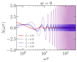
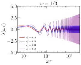
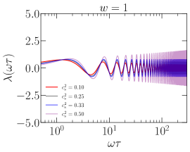
Figure 2: Evolution of the sound wave perturbations $\lambda$ for an arbitrary choice of the initial conditions, $c_{2}=0$. Free-propagating waves are found when $c_{\rm s}^{2}=1/3$.

3.6 Imperfect fluids

The zero-th order approximation in hydrodynamics has been used in section 3 to characterize perfect fluids. It is valid under the assumption that the distribution function $f$ of the fluid particles is the one found in thermal equilibrium, i.e., the Maxwell-Boltzmann distribution (see [9] for details on the relativistic equilibrium distribution functions). The perfect fluid description holds when the collisions in the system are frequent, such that they drive the fluid parcels to local thermal equilibrium (LTE) in a time-scale $l_{\rm mfp}/v$ that is shorter than those characterizing the fluid, being $v$ the typical particle velocity. This corresponds to the limit of small Knudsen number, Kn $=l_{\rm mfp}/L\ll 1$, where $l_{\rm mfp}$ is defined as the mean free path of the fluid particles and $L$ a characteristic length scale of the fluid fields.

In section 3.6.1, the distribution function is expanded using the Knudsen number as the perturbative parameter, following Chapman-Enskog theory [69]. This allows to describe imperfect fluids in the first order hydrodynamic approximation, leading to Navier-Stokes equations describing viscosity, and to heat fluxes, described by Fourier’s law of conductivity. In section 3.6.2, the Navier-Stokes and Fourier’s heat flux are presented in a covariant relativistic formulation, following the classical irreversible thermodynamics (CIT) approach, also known as first-order theories [70, 56, 9]. A known problem of the CIT approach is that it leads to fluid perturbations that are allowed to propagate at unbounded speeds, violating the postulates of special relativity. This is a consequence of the parabolic nature of the diffusion operators that appear in Navier-Stokes viscosity $\nu\mathchoice{\mbox{\boldmath$\displaystyle\nabla$}}{\mbox{\boldmath$\textstyle\nabla$}}{\mbox{\boldmath$\scriptstyle\nabla$}}{\mbox{\boldmath$\scriptscriptstyle\nabla$}}{}^{2}\mathchoice{\mbox{\boldmath$\displaystyle u$}}{\mbox{\boldmath$\textstyle u$}}{\mbox{\boldmath$\scriptstyle u$}}{\mbox{\boldmath$\scriptscriptstyle u$}}{}$ and Fourier’s law $\kappa\mathchoice{\mbox{\boldmath$\displaystyle\nabla$}}{\mbox{\boldmath$\textstyle\nabla$}}{\mbox{\boldmath$\scriptstyle\nabla$}}{\mbox{\boldmath$\scriptscriptstyle\nabla$}}{}^{2}T$, being $\nu$ and $\kappa$ the shear viscous coefficient and the conductivity.

A possible solution is to introduce relaxation times $\tau_{r}$ to the equations, motivated by the results found in kinetic theory, as proposed in [71] for the heat flux,

$$\tau_{r}\partial_{\tau}\mathchoice{\mbox{\boldmath$\displaystyle q$}}{\mbox{\boldmath$\textstyle q$}}{\mbox{\boldmath$\scriptstyle q$}}{\mbox{\boldmath$\scriptscriptstyle q$}}{}+\mathchoice{\mbox{\boldmath$\displaystyle q$}}{\mbox{\boldmath$\textstyle q$}}{\mbox{\boldmath$\scriptstyle q$}}{\mbox{\boldmath$\scriptscriptstyle q$}}{}=-\kappa\mathchoice{\mbox{\boldmath$\displaystyle\nabla$}}{\mbox{\boldmath$\textstyle\nabla$}}{\mbox{\boldmath$\scriptstyle\nabla$}}{\mbox{\boldmath$\scriptscriptstyle\nabla$}}{}^{2}T\,,$$ (1.2daaacahdeftvwacaeauaxbjbnbrbubwcbcdcecf)

where the inclusion of the $\tau_{r}\partial_{\tau}\mathchoice{\mbox{\boldmath$\displaystyle q$}}{\mbox{\boldmath$\textstyle q$}}{\mbox{\boldmath$\scriptstyle q$}}{\mbox{\boldmath$\scriptscriptstyle q$}}{}$ term makes the equation hyperbolic, and hence, respecting causality, as it introduces a response time to changes in the temperature. Following the pioneer work of [72, 73], leading to the Israel-Stewart equations, dynamical equations for the transport coefficients (e.g., shear and bulk viscosity, and conductivity) are introduced together with relaxation times, also known as the Maxwell-Cattaneo form of the relativistic viscous hydrodynamic equations [9, 54]. For example, the deviatoric viscous tensor is described using the following dynamical equation

$$\tau_{\Pi}\partial_{\tau}\Pi^{ij}+\Pi^{ij}=\tilde{\Pi}^{ij}\,,$$ (1.2daaacahdeftvwacaeauaxbjbnbrbubwcbcdcecg)

where $\tilde{\Pi}_{ij}$ corresponds to the deviatoric viscous tensor found under the CIT approach (see section 3.6.2). These models are known as extended irreversible thermodynamics (EIT), or second-order theories. They are an active topic of research (see the review [54]) and go beyond the scope of this work.

For simplicity, we will restrict ourselves to the CIT approach to describe Navier-Stokes viscosity and will ignore heat fluxes in the following. Under this simplified approach, one then needs to carefully check if superluminal velocity fields appear in the simulations as a consequence of the viscous modelling. Furthermore, we will only consider the Navier-Stokes contribution to the momentum equation in the subrelativistic limit for simplicity. For simulations of early Universe MHD after the onset of radiation domination and before recombination, the actual values of the viscosity are very small [74, 20], usually orders of magnitude below values of the viscous coefficients that can be realized in a realistic simulation (see, e.g., [10, 13, 25, 41, 32, 37, 38, 44]). Therefore, a viscous term is usually introduced to provide stability to direct numerical simulations, by introducing a damping scale near the Nyquist frequency, which realistically reproduces the large-scale dynamics as long as the resolution is enough to provide a developed inertial range between the integral and the damping scale, determined by the Reynolds number. In these situations, as the simulations are not resolving for the microphysics at small scales, the relativistic description is not expected to affect the dynamics and this approach is sufficient.

For further details on relativistic hydrodynamics of imperfect fluids we recommend the reader [54, 9] and references therein.

3.6.1 First-order imperfect subrelativistic fluids

Viscous effects and heat fluxes arise due to collisions of the fluid particles that deviate the distribution function with respect to LTE, such that ${\rm\,d}f/{\rm\,d}t\neq 0$. The resulting distribution function can be expanded in terms of the Knudsen number

$$f(X^{\mu},p^{\mu})=f_{0}(X^{\mu},p^{\mu})+\delta f(X^{\mu},p^{\mu})+{\cal O}({\rm Kn}^{2})\,,$$ (1.2daaacahdeftvwacaeauaxbjbnbrbubwcbcdcech)

where $p^{\mu}$ is the four-momentum, $f_{0}$ is the LTE distribution (e.g., Maxwell-Boltzmann, or Maxwell-Jüttner in the relativistic limit [9]) and $\delta f$ is the first-order perturbation in the distribution function. This approach corresponds to Chapman-Enskog theory [69]. It provides a hydrodynamic description for imperfect fluids using the Knudsen number as the perturbative parameter. In particular, the Knudsen numbers based on the shear stress and the heat flux yield Navier-Stokes viscosity and Fourier law’s conductivity, respectively. In the subrelativistic limit, the contribution to the momentum equation due to first-order imperfect fluids is described by an additional contribution to the stress-energy tensor $T_{ij}=T_{ij}^{\rm pf}-\Pi_{ij}$, where $\Pi_{ij}$ is the deviatoric viscous stress tensor [56, 74, 68, 9, 75],

$$\frac{\Pi^{ij}}{p+\rho}=2\,\nu\,\sigma^{ij}+\zeta\,\theta\,\delta^{ij}\,,$$ (1.2daaacahdeftvwacaeauaxbjbnbrbubwcbcdceci)

$\theta=\mathchoice{\mbox{\boldmath$\displaystyle\nabla$}}{\mbox{\boldmath$\textstyle\nabla$}}{\mbox{\boldmath$\scriptstyle\nabla$}}{\mbox{\boldmath$\scriptscriptstyle\nabla$}}{}\cdot\mathchoice{\mbox{\boldmath$\displaystyle u$}}{\mbox{\boldmath$\textstyle u$}}{\mbox{\boldmath$\scriptstyle u$}}{\mbox{\boldmath$\scriptscriptstyle u$}}{}$ is the fluid expansion scalar, $\sigma^{ij}=S^{ij}-{\textstyle{1\over 3}}\theta\delta^{ij}$, and $S^{ij}={\textstyle{1\over 2}}(\partial^{i}u^{j}+\partial^{j}u^{i})$ is the rate-of-strain tensor. The (kinematic) shear and bulk viscous coefficients are $\nu$ and $\zeta$, respectively.

A particular choice of the viscous coefficients is such that the stress-energy tensor trace is zero, keeping the conformal invariance discussed in section 3. This is accomplished when the bulk viscosity vanishes, $\zeta=0$, as $\sigma^{i}_{\ i}=0$. This is usually known as the Stokes assumption [68]. We note that the comoving rate-of-strain tensor is

$$\tilde{\Pi}^{ij}=a^{6}\Pi^{ij}\sim a^{6}\,\nu\,\rho\,\frac{\partial U^{j}}{\partial X_{i}}=a^{-1}\,\nu\,\tilde{\rho}\,\mathchoice{\mbox{\boldmath$\displaystyle\nabla$}}{\mbox{\boldmath$\textstyle\nabla$}}{\mbox{\boldmath$\scriptstyle\nabla$}}{\mbox{\boldmath$\scriptscriptstyle\nabla$}}{}\mathchoice{\mbox{\boldmath$\displaystyle u$}}{\mbox{\boldmath$\textstyle u$}}{\mbox{\boldmath$\scriptstyle u$}}{\mbox{\boldmath$\scriptscriptstyle u$}}{}\,.$$ (1.2daaacahdeftvwacaeauaxbjbnbrbubwcbcdcecj)

Hence, an appropiate choice of the comoving kinematic viscosity is $\tilde{\nu}=\nu/a$.

The contributions to the energy equation due to heat fluxes $q_{i}$ is described by an additional contribution to $T_{i0}=T_{i0}^{\rm pf}+q_{i}$, and $q_{i}=-\kappa\,\partial_{i}T$, where $\kappa$ is the thermal conductivity. Furthermore, a viscous dissipation term $\Pi^{ij}S_{ij}$ appears in the right-hand side of the energy equation [68, 9]. It represents the irreversible conversion of mechanical to thermal energy through the action of viscosity. The inclusion of these terms to the equations described in previous sections for a perfect fluid leads to the Navier-Stokes equations, together with Fourier’s law of heat conduction. As these correspond to out-of-equilibrium effects, both $\mathchoice{\mbox{\boldmath$\displaystyle\nabla$}}{\mbox{\boldmath$\textstyle\nabla$}}{\mbox{\boldmath$\scriptstyle\nabla$}}{\mbox{\boldmath$\scriptscriptstyle\nabla$}}{}\cdot\mathchoice{\mbox{\boldmath$\displaystyle q$}}{\mbox{\boldmath$\textstyle q$}}{\mbox{\boldmath$\scriptstyle q$}}{\mbox{\boldmath$\scriptscriptstyle q$}}{}$ and $\Pi^{ij}S_{ij}$ are irreversible processes leading to an increase of entropy.

Conservation form of Navier-Stokes equations

In MHD simulations of the primordial plasma in the radiation-dominated era of the early Universe (see, e.g., [10, 25, 32]), Navier-Stokes description for viscosity has been used (ignoring heat fluxes), which leads to the inclusion of (1.2daaacahdeftvwacaeauaxbjbnbrbubwcbcdceci) in the momentum equation [see (1.2daaacahdeftvwacaeai)],

$$\partial_{\tau}\tilde{T}^{0i}_{\rm pf}+\partial_{j}\tilde{T}^{ij}_{\rm pf}=\tilde{f}_{H}^{i}+\partial_{j}\tilde{\Pi}^{ij}=\tilde{f}_{H}^{i}+\tilde{f}^{i}_{\rm visc}\,.$$ (1.2daaacahdeftvwacaeauaxbjbnbrbubwcbcdceck)

Then, the viscous force corresponds to the divergence of the deviatoric tensor and takes the following form, where we already normalize with the enthalpy $\tilde{p}+\tilde{\rho}$ as this term will appear in the momentum equation, and assume a homogeneous $\tilde{\nu}$ for simplicity,

$$\frac{\partial_{j}\tilde{\Pi}_{ij}}{\tilde{p}+\tilde{\rho}}=\frac{\mathchoice{\mbox{\boldmath$\displaystyle\tilde{f}$}}{\mbox{\boldmath$\textstyle\tilde{f}$}}{\mbox{\boldmath$\scriptstyle\tilde{f}$}}{\mbox{\boldmath$\scriptscriptstyle\tilde{f}$}}{}_{\rm visc}}{\tilde{p}+\tilde{\rho}}=\frac{\mathchoice{\mbox{\boldmath$\displaystyle\nabla$}}{\mbox{\boldmath$\textstyle\nabla$}}{\mbox{\boldmath$\scriptstyle\nabla$}}{\mbox{\boldmath$\scriptscriptstyle\nabla$}}{}\cdot\bigl{(}2\,\tilde{\nu}\,[\tilde{p}+\tilde{\rho}]\,\boldsymbol{\sigma}\bigr{)}}{\tilde{p}+\tilde{\rho}}=\tilde{\nu}\,\Bigl{(}\mathchoice{\mbox{\boldmath$\displaystyle\nabla$}}{\mbox{\boldmath$\textstyle\nabla$}}{\mbox{\boldmath$\scriptstyle\nabla$}}{\mbox{\boldmath$\scriptscriptstyle\nabla$}}{}^{2}\mathchoice{\mbox{\boldmath$\displaystyle u$}}{\mbox{\boldmath$\textstyle u$}}{\mbox{\boldmath$\scriptstyle u$}}{\mbox{\boldmath$\scriptscriptstyle u$}}{}+{\textstyle{1\over 3}}\mathchoice{\mbox{\boldmath$\displaystyle\nabla$}}{\mbox{\boldmath$\textstyle\nabla$}}{\mbox{\boldmath$\scriptstyle\nabla$}}{\mbox{\boldmath$\scriptscriptstyle\nabla$}}{}\theta+2\,(\boldsymbol{\sigma}\cdot\mathchoice{\mbox{\boldmath$\displaystyle\nabla$}}{\mbox{\boldmath$\textstyle\nabla$}}{\mbox{\boldmath$\scriptstyle\nabla$}}{\mbox{\boldmath$\scriptscriptstyle\nabla$}}{})\ln[\tilde{p}+\tilde{\rho}]\Bigr{)}\,.$$ (1.2daaacahdeftvwacaeauaxbjbnbrbubwcbcdcecl)

Note that the comoving shear viscosity is $\tilde{\nu}=a^{-1}\nu$, using the conformal transformation $\tilde{\Pi}^{ij}=a^{6}\Pi^{ij}$. To solve this system in the conservation form, one can follow the procedure described in section 3.3 to relate $\tilde{T}^{ij}_{\rm pf}$ to $\tilde{T}^{0\mu}_{\rm pf}$, and then construct the viscous force from (1.2daaacahdeftvwacaeauaxbjbnbrbubwcbcdcecl), where the velocity field can be obtained from $\tilde{T}^{0\mu}_{\rm pf}$ using (1.2daaacahdeftvwacaeao). Then, the viscous force can be included in the force array $F^{a}$ in (1.2daaacahdeftvwacaeak), as well as any additional forces that might be exerted on the fluid (e.g., electromagnetic fields, as we will see in section 5).

The energy equation would also include the effect of viscous dissipation [see (1.2daaacahdeftvwacaeai)],

$$\partial_{\tau}\tilde{T}^{0i}_{\rm pf}+\partial_{j}\tilde{T}^{0i}_{\rm pf}=\tilde{f}_{H}^{0}+\tilde{\Pi}_{ij}S^{ij}=\tilde{f}_{H}^{0}+\tilde{f}_{\rm visc}^{0}\,,$$ (1.2daaacahdeftvwacaeauaxbjbnbrbubwcbcdcecm)

where

$$\frac{\tilde{f}_{\rm visc}^{0}}{\tilde{p}+\tilde{\rho}}=2\,\tilde{\nu}\,S^{ij}S_{ij}-{\textstyle{2\over 3}}\,\tilde{\nu}\,\theta^{2}\,.$$ (1.2daaacahdeftvwacaeauaxbjbnbrbubwcbcdcecn)

Non-conservation form of Navier-Stokes equations

In the following, we include the viscous force $\tilde{f}_{\rm visc}^{\mu}$ in the non-conservation form of the energy and momentum equations, studied for perfect fluids in section 3.4. To find the effect of viscous forces, we first note that this term leads to an additional term in the evolution equation of the Lorentz factor [see (1.2daaacahdeftvwacaeauaxbi), where we can generalize $\tilde{f}_{H}^{\mu}\to\tilde{f}_{H}^{\mu}+\tilde{f}^{\mu}_{\rm visc}$ due to the modifications in the momentum and energy equations,

$$\partial_{\tau}\ln\gamma^{2}\to\partial_{\tau}\ln\gamma^{2}+\frac{2}{1+c_{\rm s}^{2}}\,\frac{1+c_{\rm s}^{2}u^{2}}{1-c_{\rm s}^{2}u^{2}}\,\frac{\mathchoice{\mbox{\boldmath$\displaystyle u$}}{\mbox{\boldmath$\textstyle u$}}{\mbox{\boldmath$\scriptstyle u$}}{\mbox{\boldmath$\scriptscriptstyle u$}}{}\cdot\mathchoice{\mbox{\boldmath$\displaystyle\tilde{f}$}}{\mbox{\boldmath$\textstyle\tilde{f}$}}{\mbox{\boldmath$\scriptstyle\tilde{f}$}}{\mbox{\boldmath$\scriptscriptstyle\tilde{f}$}}{}_{\rm visc}}{\tilde{\rho}}-\frac{u^{2}}{1-c_{\rm s}^{2}u^{2}}\frac{\tilde{f}_{\rm visc}^{0}}{\tilde{\rho}}\,,$$ (1.2daaacahdeftvwacaeauaxbjbnbrbubwcbcdceco)

where the viscous forces are given by (1.2daaacahdeftvwacaeauaxbjbnbrbubwcbcdcecl) and (1.2daaacahdeftvwacaeauaxbjbnbrbubwcbcdcecn). While the term corresponding to the viscous energy dissipation $\tilde{f}_{\rm visc}^{0}$ is relativistic, the term corresponding to the viscous force $\mathchoice{\mbox{\boldmath$\displaystyle\tilde{f}$}}{\mbox{\boldmath$\textstyle\tilde{f}$}}{\mbox{\boldmath$\scriptstyle\tilde{f}$}}{\mbox{\boldmath$\scriptscriptstyle\tilde{f}$}}{}_{\rm visc}$ does not vanish in general in the subrelativistic limit. Therefore, its inclusion can impact the energy and momentum equations and has not been considered in previous work. However, when the shear viscosity is small, this term can be neglected.

The resulting relativistic energy and momentum equations are

$$\partial_{\tau}\ln\tilde{\rho}=-\frac{1+c_{\rm s}^{2}}{1-c_{\rm s}^{2}u^{2}}\biggl{[}\mathchoice{\mbox{\boldmath$\displaystyle\nabla$}}{\mbox{\boldmath$\textstyle\nabla$}}{\mbox{\boldmath$\scriptstyle\nabla$}}{\mbox{\boldmath$\scriptscriptstyle\nabla$}}{}\cdot\mathchoice{\mbox{\boldmath$\displaystyle u$}}{\mbox{\boldmath$\textstyle u$}}{\mbox{\boldmath$\scriptstyle u$}}{\mbox{\boldmath$\scriptscriptstyle u$}}{}+\frac{1-c_{\rm s}^{2}}{1+c_{\rm s}^{2}}\,\bigl{(}\mathchoice{\mbox{\boldmath$\displaystyle u$}}{\mbox{\boldmath$\textstyle u$}}{\mbox{\boldmath$\scriptstyle u$}}{\mbox{\boldmath$\scriptscriptstyle u$}}{}\cdot\mathchoice{\mbox{\boldmath$\displaystyle\nabla$}}{\mbox{\boldmath$\textstyle\nabla$}}{\mbox{\boldmath$\scriptstyle\nabla$}}{\mbox{\boldmath$\scriptscriptstyle\nabla$}}{}\bigr{)}\ln\tilde{\rho}\biggr{]}+{\cal F}_{H}^{0}$$

$$+\frac{1}{1-c_{\rm s}^{2}u^{2}}\biggl{[}\frac{\tilde{f}_{\rm visc}^{0}}{\tilde{\rho}}(1+u^{2})-2\,\frac{\mathchoice{\mbox{\boldmath$\displaystyle u$}}{\mbox{\boldmath$\textstyle u$}}{\mbox{\boldmath$\scriptstyle u$}}{\mbox{\boldmath$\scriptscriptstyle u$}}{}\cdot\mathchoice{\mbox{\boldmath$\displaystyle\tilde{f}$}}{\mbox{\boldmath$\textstyle\tilde{f}$}}{\mbox{\boldmath$\scriptstyle\tilde{f}$}}{\mbox{\boldmath$\scriptscriptstyle\tilde{f}$}}{}_{\rm visc}}{\tilde{\rho}}\biggr{]}\,,$$ (1.2daaacahdeftvwacaeauaxbjbnbrbubwcbcdcecpa)

$$\partial_{\tau}\mathchoice{\mbox{\boldmath$\displaystyle u$}}{\mbox{\boldmath$\textstyle u$}}{\mbox{\boldmath$\scriptstyle u$}}{\mbox{\boldmath$\scriptscriptstyle u$}}{}+\bigl{(}\mathchoice{\mbox{\boldmath$\displaystyle u$}}{\mbox{\boldmath$\textstyle u$}}{\mbox{\boldmath$\scriptstyle u$}}{\mbox{\boldmath$\scriptscriptstyle u$}}{}\cdot\mathchoice{\mbox{\boldmath$\displaystyle\nabla$}}{\mbox{\boldmath$\textstyle\nabla$}}{\mbox{\boldmath$\scriptstyle\nabla$}}{\mbox{\boldmath$\scriptscriptstyle\nabla$}}{}\bigr{)}\mathchoice{\mbox{\boldmath$\displaystyle u$}}{\mbox{\boldmath$\textstyle u$}}{\mbox{\boldmath$\scriptstyle u$}}{\mbox{\boldmath$\scriptscriptstyle u$}}{}=\frac{\mathchoice{\mbox{\boldmath$\displaystyle u$}}{\mbox{\boldmath$\textstyle u$}}{\mbox{\boldmath$\scriptstyle u$}}{\mbox{\boldmath$\scriptscriptstyle u$}}{}}{(1-c_{\rm s}^{2}u^{2})\gamma^{2}}\biggl{[}c_{\rm s}^{2}\,\mathchoice{\mbox{\boldmath$\displaystyle\nabla$}}{\mbox{\boldmath$\textstyle\nabla$}}{\mbox{\boldmath$\scriptstyle\nabla$}}{\mbox{\boldmath$\scriptscriptstyle\nabla$}}{}\cdot\mathchoice{\mbox{\boldmath$\displaystyle u$}}{\mbox{\boldmath$\textstyle u$}}{\mbox{\boldmath$\scriptstyle u$}}{\mbox{\boldmath$\scriptscriptstyle u$}}{}+c_{\rm s}^{2}\frac{1-c_{\rm s}^{2}}{1+c_{\rm s}^{2}}(\mathchoice{\mbox{\boldmath$\displaystyle u$}}{\mbox{\boldmath$\textstyle u$}}{\mbox{\boldmath$\scriptstyle u$}}{\mbox{\boldmath$\scriptscriptstyle u$}}{}\cdot\mathchoice{\mbox{\boldmath$\displaystyle\nabla$}}{\mbox{\boldmath$\textstyle\nabla$}}{\mbox{\boldmath$\scriptstyle\nabla$}}{\mbox{\boldmath$\scriptscriptstyle\nabla$}}{})\ln\tilde{\rho}+{\cal H}(3c_{\rm s}^{2}-1)-\frac{\tilde{f}_{\rm visc}^{0}}{\tilde{\rho}}\biggr{]}$$

$$+\frac{\mathchoice{\mbox{\boldmath$\displaystyle u$}}{\mbox{\boldmath$\textstyle u$}}{\mbox{\boldmath$\scriptstyle u$}}{\mbox{\boldmath$\scriptscriptstyle u$}}{}}{(1-c_{\rm s}^{2}u^{2})\gamma^{2}}\,\frac{2c_{\rm s}^{2}}{1+c_{\rm s}^{2}}\,\frac{\mathchoice{\mbox{\boldmath$\displaystyle u$}}{\mbox{\boldmath$\textstyle u$}}{\mbox{\boldmath$\scriptstyle u$}}{\mbox{\boldmath$\scriptscriptstyle u$}}{}\cdot\mathchoice{\mbox{\boldmath$\displaystyle\tilde{f}$}}{\mbox{\boldmath$\textstyle\tilde{f}$}}{\mbox{\boldmath$\scriptstyle\tilde{f}$}}{\mbox{\boldmath$\scriptscriptstyle\tilde{f}$}}{}_{\rm visc}}{\tilde{\rho}}-\frac{c_{\rm s}^{2}}{1+c_{\rm s}^{2}}\frac{\mathchoice{\mbox{\boldmath$\displaystyle\nabla$}}{\mbox{\boldmath$\textstyle\nabla$}}{\mbox{\boldmath$\scriptstyle\nabla$}}{\mbox{\boldmath$\scriptscriptstyle\nabla$}}{}\ln\tilde{\rho}}{\gamma^{2}}+\frac{1}{1+c_{\rm s}^{2}}\,\frac{\mathchoice{\mbox{\boldmath$\displaystyle\tilde{f}$}}{\mbox{\boldmath$\textstyle\tilde{f}$}}{\mbox{\boldmath$\scriptstyle\tilde{f}$}}{\mbox{\boldmath$\scriptscriptstyle\tilde{f}$}}{}_{\rm visc}}{\tilde{\rho}\gamma^{2}}\,.$$ (1.2daaacahdeftvwacaeauaxbjbnbrbubwcbcdcecpb)

Note that this system of equations can be generalized to any set of external forces $\tilde{f}^{\mu}_{\rm tot}$ by setting $\tilde{f}_{\rm visc}^{\mu}\to\tilde{f}_{\rm tot}^{\mu}$.

In the subrelativistic limit, we find

$$\partial_{\tau}\ln\tilde{\rho}=-(1+c_{\rm s}^{2})\,\mathchoice{\mbox{\boldmath$\displaystyle\nabla$}}{\mbox{\boldmath$\textstyle\nabla$}}{\mbox{\boldmath$\scriptstyle\nabla$}}{\mbox{\boldmath$\scriptscriptstyle\nabla$}}{}\cdot\mathchoice{\mbox{\boldmath$\displaystyle u$}}{\mbox{\boldmath$\textstyle u$}}{\mbox{\boldmath$\scriptstyle u$}}{\mbox{\boldmath$\scriptscriptstyle u$}}{}-(1-c_{\rm s}^{2})\bigl{(}\mathchoice{\mbox{\boldmath$\displaystyle u$}}{\mbox{\boldmath$\textstyle u$}}{\mbox{\boldmath$\scriptstyle u$}}{\mbox{\boldmath$\scriptscriptstyle u$}}{}\cdot\mathchoice{\mbox{\boldmath$\displaystyle\nabla$}}{\mbox{\boldmath$\textstyle\nabla$}}{\mbox{\boldmath$\scriptstyle\nabla$}}{\mbox{\boldmath$\scriptscriptstyle\nabla$}}{}\bigr{)}\ln\tilde{\rho}+{\cal H}\bigl{[}\beta-3\,(1+c_{\rm s}^{2})\bigr{]}$$

$$+\frac{\tilde{f}_{\rm visc}^{0}}{\tilde{\rho}}-2\,\frac{\mathchoice{\mbox{\boldmath$\displaystyle u$}}{\mbox{\boldmath$\textstyle u$}}{\mbox{\boldmath$\scriptstyle u$}}{\mbox{\boldmath$\scriptscriptstyle u$}}{}\cdot\mathchoice{\mbox{\boldmath$\displaystyle\tilde{f}$}}{\mbox{\boldmath$\textstyle\tilde{f}$}}{\mbox{\boldmath$\scriptstyle\tilde{f}$}}{\mbox{\boldmath$\scriptscriptstyle\tilde{f}$}}{}_{\rm visc}}{\tilde{\rho}}\,,$$ (1.2daaacahdeftvwacaeauaxbjbnbrbubwcbcdcecpcqa)

$$\partial_{\tau}\mathchoice{\mbox{\boldmath$\displaystyle u$}}{\mbox{\boldmath$\textstyle u$}}{\mbox{\boldmath$\scriptstyle u$}}{\mbox{\boldmath$\scriptscriptstyle u$}}{}+\bigl{(}\mathchoice{\mbox{\boldmath$\displaystyle u$}}{\mbox{\boldmath$\textstyle u$}}{\mbox{\boldmath$\scriptstyle u$}}{\mbox{\boldmath$\scriptscriptstyle u$}}{}\cdot\mathchoice{\mbox{\boldmath$\displaystyle\nabla$}}{\mbox{\boldmath$\textstyle\nabla$}}{\mbox{\boldmath$\scriptstyle\nabla$}}{\mbox{\boldmath$\scriptscriptstyle\nabla$}}{}\bigr{)}\mathchoice{\mbox{\boldmath$\displaystyle u$}}{\mbox{\boldmath$\textstyle u$}}{\mbox{\boldmath$\scriptstyle u$}}{\mbox{\boldmath$\scriptscriptstyle u$}}{}=\mathchoice{\mbox{\boldmath$\displaystyle u$}}{\mbox{\boldmath$\textstyle u$}}{\mbox{\boldmath$\scriptstyle u$}}{\mbox{\boldmath$\scriptscriptstyle u$}}{}\biggl{[}c_{\rm s}^{2}\,\mathchoice{\mbox{\boldmath$\displaystyle\nabla$}}{\mbox{\boldmath$\textstyle\nabla$}}{\mbox{\boldmath$\scriptstyle\nabla$}}{\mbox{\boldmath$\scriptscriptstyle\nabla$}}{}\cdot\mathchoice{\mbox{\boldmath$\displaystyle u$}}{\mbox{\boldmath$\textstyle u$}}{\mbox{\boldmath$\scriptstyle u$}}{\mbox{\boldmath$\scriptscriptstyle u$}}{}+c_{\rm s}^{2}\,\frac{1-c_{\rm s}^{2}}{1+c_{\rm s}^{2}}\,(\mathchoice{\mbox{\boldmath$\displaystyle u$}}{\mbox{\boldmath$\textstyle u$}}{\mbox{\boldmath$\scriptstyle u$}}{\mbox{\boldmath$\scriptscriptstyle u$}}{}\cdot\mathchoice{\mbox{\boldmath$\displaystyle\nabla$}}{\mbox{\boldmath$\textstyle\nabla$}}{\mbox{\boldmath$\scriptstyle\nabla$}}{\mbox{\boldmath$\scriptscriptstyle\nabla$}}{})\ln\tilde{\rho}+{\cal H}(3c_{\rm s}^{2}-1)-\frac{\tilde{f}_{\rm visc}^{0}}{\tilde{\rho}}\biggr{]}$$

$$+\mathchoice{\mbox{\boldmath$\displaystyle u$}}{\mbox{\boldmath$\textstyle u$}}{\mbox{\boldmath$\scriptstyle u$}}{\mbox{\boldmath$\scriptscriptstyle u$}}{}\,\frac{2\,c_{\rm s}^{2}}{1+c_{\rm s}^{2}}\,\frac{\mathchoice{\mbox{\boldmath$\displaystyle u$}}{\mbox{\boldmath$\textstyle u$}}{\mbox{\boldmath$\scriptstyle u$}}{\mbox{\boldmath$\scriptscriptstyle u$}}{}\cdot\mathchoice{\mbox{\boldmath$\displaystyle\tilde{f}$}}{\mbox{\boldmath$\textstyle\tilde{f}$}}{\mbox{\boldmath$\scriptstyle\tilde{f}$}}{\mbox{\boldmath$\scriptscriptstyle\tilde{f}$}}{}_{\rm visc}}{\tilde{\rho}}-\frac{c_{\rm s}^{2}}{1+c_{\rm s}^{2}}\mathchoice{\mbox{\boldmath$\displaystyle\nabla$}}{\mbox{\boldmath$\textstyle\nabla$}}{\mbox{\boldmath$\scriptstyle\nabla$}}{\mbox{\boldmath$\scriptscriptstyle\nabla$}}{}\ln\tilde{\rho}+\frac{1}{1+c_{\rm s}^{2}}\frac{\mathchoice{\mbox{\boldmath$\displaystyle\tilde{f}$}}{\mbox{\boldmath$\textstyle\tilde{f}$}}{\mbox{\boldmath$\scriptstyle\tilde{f}$}}{\mbox{\boldmath$\scriptscriptstyle\tilde{f}$}}{}_{\rm visc}}{\tilde{\rho}}\,,$$ (1.2daaacahdeftvwacaeauaxbjbnbrbubwcbcdcecpcqb)

where the last term in the momentum equation is the term that had been included in previous work (see, e.g., [10, 25, 32]). We note that $\mathchoice{\mbox{\boldmath$\displaystyle\tilde{f}$}}{\mbox{\boldmath$\textstyle\tilde{f}$}}{\mbox{\boldmath$\scriptstyle\tilde{f}$}}{\mbox{\boldmath$\scriptscriptstyle\tilde{f}$}}{}_{\rm visc}$ is proportional to $\tilde{\rho}\,(1+c_{\rm s}^{2})$ [see (1.2daaacahdeftvwacaeauaxbjbnbrbubwcbcdcecl)], such that the prefactors $1/[(1+c_{\rm s}^{2})\tilde{\rho}]$ in the momentum equations cancel out. On the other hand, the dissipation and work done by the viscous forces have not been included in previous work, under the assumption that the shear viscosity is very small [74].

3.6.2 Covariant formulation of Navier-Stokes viscosity

In the following, the Navier-Stokes description of viscosity in an appropriate relativistic covariant formulation is described. For a covariant formulation of the heat transfer contribution to the stress-energy tensor, see [1, 11]. The viscous contribution to the stress-energy tensor is described by the deviatoric viscous stress $\Pi^{\mu\nu}$ in the following way [4, 11, 76, 54],

$$\Pi^{\mu\nu}=2\nu\sigma^{\mu\nu}+\zeta\theta h^{\mu\nu}\,,\qquad\sigma^{\mu\nu}=S^{\mu\nu}-\frac{1}{3}\theta h^{\mu\nu},$$ (1.2daaacahdeftvwacaeauaxbjbnbrbubwcbcdcecpcqcr)

where $\theta=D_{\mu}U_{\mu}$ is the relativistic dilatational coefficient. $S^{\mu\nu}$ is the relativistic rate-of-strain tensor,

$$S^{\mu\nu}=\frac{1}{2}\bigl{(}h^{\alpha\nu}D_{\alpha}U^{\mu}+h^{\alpha\mu}D_{\alpha}U^{\nu}\bigr{)}\,,$$ (1.2daaacahdeftvwacaeauaxbjbnbrbubwcbcdcecpcqcs)

where $h^{\mu\nu}=g^{\mu\nu}+U^{\mu}U^{\nu}$ is the spatial projection tensor [76, 77, 9]. We can rearrange (1.2daaacahdeftvwacaeauaxbjbnbrbubwcbcdcecpcqcr) in the following way

$$\Pi^{\mu\nu}=2\nu S^{\mu\nu}+\theta h^{\mu\nu}\biggl{(}\zeta-\frac{2}{3}\nu\biggr{)}.$$ (1.2daaacahdeftvwacaeauaxbjbnbrbubwcbcdcecpcqct)

The term $\sigma^{\mu\nu}$ is traceless by definition,

$$\sigma^{\mu}_{\ \,\mu}=S^{\mu}_{\ \,\mu}-{\textstyle{1\over 3}}\theta h^{\mu}_{\ \mu}=0\ ,$$ (1.2daaacahdeftvwacaeauaxbjbnbrbubwcbcdcecpcqcu)

while the bulk viscosity yields an additional term with trace $\zeta\theta h^{\mu}_{\ \mu}=3\zeta\theta$, which corresponds to the trace of the viscous stress tensor, in the same way as for the relativistic Navier-Stokes viscosity,

$$\Pi^{\mu}_{\ \mu}=3\,\zeta\,\theta\ .$$ (1.2daaacahdeftvwacaeauaxbjbnbrbubwcbcdcecpcqcv)

Therefore, only when the bulk viscosity is zero, the equations of motion of a radiation-dominated imperfect fluid in an expanding background are conformally flat [12]. As done in the previous section, we will assume the Stokes’ hypothesis, setting $\zeta=0$,

$$\Pi^{\mu\nu}=2\nu S^{\mu\nu}-{\textstyle{2\over 3}}\theta\nu h^{\mu\nu}\,,$$ (1.2daaacahdeftvwacaeauaxbjbnbrbubwcbcdcecpcqcw)

which corresponds to the relativistic extension of (1.2daaacahdeftvwacaeauaxbjbnbrbubwcbcdceci). Subtracting the deviatoric tensor $\tilde{\Pi}^{\mu\nu}$ to the stress-energy tensor of a perfect fluid $\tilde{T}^{\mu\nu}=\tilde{T}^{\mu\nu}_{\rm pf}-\tilde{\Pi}^{\mu\nu}$, we can express the relativistic energy and momentum equations from (1.2daaacahdeftvwacaeai),

$$\partial_{\tau}\tilde{T}^{0\mu}_{\rm pf}+\partial_{i}\tilde{T}^{i\mu}_{\rm pf}=\tilde{f}_{H}^{\mu}+\partial_{i}\tilde{\Pi}^{\mu i}=\tilde{f}_{H}^{\mu}+\tilde{f}_{\rm visc}^{\mu}\,.$$ (1.2daaacahdeftvwacaeauaxbjbnbrbubwcbcdcecpcqcx)

The solution to this system of equations is complex as it involves time derivatives of the primitive variables in the viscous forces. The time derivatives over $\tilde{\Pi}^{00}$ and $\tilde{\Pi}^{0i}$ leads in fact to second-order derivatives of the fluid variables $\gamma$ and $\textstyle u$ in the energy and momentum equation.

4 Standard Electromagnetism: Maxwell equations

In order to describe the dynamics of charged fluids, we first need to introduce Maxwell equations in an expanding Universe that will later be coupled to the equations of motion of the fluid, following an MHD description. In the following, we set the time-like signature $(-+++)$, i.e., $m=1$, set $X^{0}=\tau$, and $\alpha=1$, for simplicity.

4.1 Faraday tensor and covariant electromagnetic fields

We will only consider the $U(1)_{\rm EM}$ sector of gauge fields as the classical electromagnetic fields, such that we describe electromagnetism at temperature scales below the electroweak symmetry breaking. At larger temperatures, the electroweak force is described by the group of symmetries $SU(2)_{\rm L}\times U(1)_{\rm Y}$. An Abelian $U(1)$ gauge field $A^{\mu}=(\chi,A^{i})$ can be described using the Faraday tensor,

$$F_{\mu\nu}=\partial_{\mu}A_{\nu}-\partial_{\nu}A_{\mu}\,,$$ (1.2daaacahdeftvwacaeauaxbjbnbrbubwcbcdcecpcqa)

which is, by definition, conformal invariant, i.e., $F_{\mu\nu}=D_{\mu}A_{\nu}-D_{\nu}A_{\mu}$. The covariant electromagnetic fields can be defined in the following way [76, 77]

$$E_{\mu}=F_{\mu\nu}\,U^{\nu}\,,\qquad B_{\mu}={\cal F}_{\mu\nu}\,U^{\nu}\,,$$ (1.2daaacahdeftvwacaeauaxbjbnbrbubwcbcdcecpcqb)

where ${\cal F}_{\mu\nu}={\textstyle{1\over 2}}E_{{\mu\nu}\alpha\beta}F^{\alpha\beta}$ is the Faraday dual tensor, and $U^{\mu}$ represents the four-velocity of the observer that measures the electromagnetic fields. This definition of the electromagnetic fields allows us to describe the fields as tensors, as the usual electromagnetic fields are not invariant under Lorentz boosts. In fact an electric field can be transformed into electric and magnetic fields, and viceversa in a boosted reference frame. We note that the covariant electric and magnetic fields are orthogonal to $U^{\mu}$,

$$E_{\mu}U^{\mu}=B_{\mu}U^{\mu}=0\,.$$ (1.2daaacahdeftvwacaeauaxbjbnbrbubwcbcdcecpcqc)

Inverting (1.2daaacahdeftvwacaeauaxbjbnbrbubwcbcdcecpcqb), one finds [76, 77]

$$F_{\mu\nu}=E_{\mu\nu\alpha\beta}B^{\alpha}U^{\beta}+U_{\mu}E_{\nu}-U_{\nu}E_{\mu}\,,\qquad{\cal F}^{\mu\nu}=E^{\mu\nu\alpha\beta}U_{\alpha}E_{\beta}+U^{\mu}B^{\nu}-U^{\nu}B^{\mu}\,.$$ (1.2daaacahdeftvwacaeauaxbjbnbrbubwcbcdcecpcqd)

The covariant and contravariant Levi-Civita tensors are

$$E^{{\mu\nu}{\alpha\beta}}=-\frac{1}{\sqrt{-g}}\varepsilon^{{\mu\nu}{\alpha\beta}}=-a^{-4}\varepsilon^{{\mu\nu}{\alpha\beta}},\qquad E_{{\mu\nu}{\alpha\beta}}=\sqrt{-g}\,\varepsilon_{{\mu\nu}{\alpha\beta}}=a^{4}\varepsilon_{{\mu\nu}{\alpha\beta}},$$ (1.2daaacahdeftvwacaeauaxbjbnbrbubwcbcdcecpcqe)

where $\varepsilon^{{\mu\nu}{\alpha\beta}}=\varepsilon_{{\mu\nu}{\alpha\beta}}$ is the usual Levi-Civita symbol, taking a value of one for even permutations of ${\mu\nu}{\alpha\beta}$ with respect to $1230$, $-1$ for odd permutations, and 0 when two indices are repeated. The contraction of two Levi-Civita tensors is

$$E^{{\mu\nu}{\lambda\sigma}}E_{{\mu\nu}{\alpha\beta}}=-\varepsilon^{{\mu\nu}{\lambda\sigma}}\varepsilon_{{\mu\nu}{\alpha\beta}}=\delta^{\lambda\sigma}_{\alpha\beta}=\delta^{\lambda}_{\alpha}\delta^{\sigma}_{\beta}-\delta^{\lambda}_{\beta}\delta^{\sigma}_{\alpha}\,.$$ (1.2daaacahdeftvwacaeauaxbjbnbrbubwcbcdcecpcqf)

In 3d we will define $E^{ijk}=E^{0ijk}$ and omit the index 0. For the comoving Hubble observer with $U^{\mu}=(1,0,0,0)/a$, we find the usual definitions of the electromagnetic fields, $E_{0}=B_{0}=0$, and

$$a\,E_{i}=F_{i0}=\nabla_{i}\chi-\partial_{\tau}A_{i}\,,\qquad a\,B_{i}={\textstyle{1\over 2}}\varepsilon_{ijk}a^{4}F^{jk}={\textstyle{1\over 2}}\varepsilon_{ijk}F_{jk}=\mathchoice{\mbox{\boldmath$\displaystyle\nabla$}}{\mbox{\boldmath$\textstyle\nabla$}}{\mbox{\boldmath$\scriptstyle\nabla$}}{\mbox{\boldmath$\scriptscriptstyle\nabla$}}{}\times\mathchoice{\mbox{\boldmath$\displaystyle A$}}{\mbox{\boldmath$\textstyle A$}}{\mbox{\boldmath$\scriptstyle A$}}{\mbox{\boldmath$\scriptscriptstyle A$}}{}\,.$$ (1.2daaacahdeftvwacaeauaxbjbnbrbubwcbcdcecpcqg)

We denote as $\chi$ the scalar potential and $\textstyle A$ the vector potential. Due to the $U(1)$ symmetry of the gauge field $A_{\mu}$, we have freedom to choose a gauge, as any transformation of the type $\chi\to\chi+\partial_{\tau}\psi$ and $\mathchoice{\mbox{\boldmath$\displaystyle A$}}{\mbox{\boldmath$\textstyle A$}}{\mbox{\boldmath$\scriptstyle A$}}{\mbox{\boldmath$\scriptscriptstyle A$}}{}\to\mathchoice{\mbox{\boldmath$\displaystyle A$}}{\mbox{\boldmath$\textstyle A$}}{\mbox{\boldmath$\scriptstyle A$}}{\mbox{\boldmath$\scriptscriptstyle A$}}{}+\mathchoice{\mbox{\boldmath$\displaystyle\nabla$}}{\mbox{\boldmath$\textstyle\nabla$}}{\mbox{\boldmath$\scriptstyle\nabla$}}{\mbox{\boldmath$\scriptscriptstyle\nabla$}}{}\psi$ maintains the physical degrees of freedom (the electric and magnetic fields) the same. Raising indices with the FLRW metric tensor $g_{\mu\nu}$ we find

$$E^{i}=a^{-2}E_{i}\,,\qquad B^{i}=a^{-2}B_{i}\,.$$ (1.2daaacahdeftvwacaeauaxbjbnbrbubwcbcdcecpcqh)

From (1.2daaacahdeftvwacaeauaxbjbnbrbubwcbcdcecpcqg), we also note that

$$F_{ij}=a^{3}\varepsilon_{ijk}B^{k}=a\,\varepsilon_{ijk}B_{k}\,.$$ (1.2daaacahdeftvwacaeauaxbjbnbrbubwcbcdcecpcqi)

The electromagnetic fields measured in the reference frame of a fluid with peculiar velocity $\mathchoice{\mbox{\boldmath$\displaystyle u$}}{\mbox{\boldmath$\textstyle u$}}{\mbox{\boldmath$\scriptstyle u$}}{\mbox{\boldmath$\scriptscriptstyle u$}}{}={\rm\,d}\mathchoice{\mbox{\boldmath$\displaystyle x$}}{\mbox{\boldmath$\textstyle x$}}{\mbox{\boldmath$\scriptstyle x$}}{\mbox{\boldmath$\scriptscriptstyle x$}}{}/{\rm\,d}\tau$ with respect to the Hubble observer, such that $U^{\mu}=\gamma(1,u_{i})/a$, have the following components

$$E^{\mu}=\gamma/a^{3}(\mathchoice{\mbox{\boldmath$\displaystyle\tilde{E}$}}{\mbox{\boldmath$\textstyle\tilde{E}$}}{\mbox{\boldmath$\scriptstyle\tilde{E}$}}{\mbox{\boldmath$\scriptscriptstyle\tilde{E}$}}{}\cdot\mathchoice{\mbox{\boldmath$\displaystyle u$}}{\mbox{\boldmath$\textstyle u$}}{\mbox{\boldmath$\scriptstyle u$}}{\mbox{\boldmath$\scriptscriptstyle u$}}{},\mathchoice{\mbox{\boldmath$\displaystyle\tilde{E}$}}{\mbox{\boldmath$\textstyle\tilde{E}$}}{\mbox{\boldmath$\scriptstyle\tilde{E}$}}{\mbox{\boldmath$\scriptscriptstyle\tilde{E}$}}{}+\mathchoice{\mbox{\boldmath$\displaystyle u$}}{\mbox{\boldmath$\textstyle u$}}{\mbox{\boldmath$\scriptstyle u$}}{\mbox{\boldmath$\scriptscriptstyle u$}}{}\times\mathchoice{\mbox{\boldmath$\displaystyle\tilde{B}$}}{\mbox{\boldmath$\textstyle\tilde{B}$}}{\mbox{\boldmath$\scriptstyle\tilde{B}$}}{\mbox{\boldmath$\scriptscriptstyle\tilde{B}$}}{})\,,$$ (1.2daaacahdeftvwacaeauaxbjbnbrbubwcbcdcecpcqja)

$$B^{\mu}=\gamma/a^{3}(\mathchoice{\mbox{\boldmath$\displaystyle\tilde{B}$}}{\mbox{\boldmath$\textstyle\tilde{B}$}}{\mbox{\boldmath$\scriptstyle\tilde{B}$}}{\mbox{\boldmath$\scriptscriptstyle\tilde{B}$}}{}\cdot\mathchoice{\mbox{\boldmath$\displaystyle u$}}{\mbox{\boldmath$\textstyle u$}}{\mbox{\boldmath$\scriptstyle u$}}{\mbox{\boldmath$\scriptscriptstyle u$}}{},\mathchoice{\mbox{\boldmath$\displaystyle\tilde{B}$}}{\mbox{\boldmath$\textstyle\tilde{B}$}}{\mbox{\boldmath$\scriptstyle\tilde{B}$}}{\mbox{\boldmath$\scriptscriptstyle\tilde{B}$}}{}-\mathchoice{\mbox{\boldmath$\displaystyle u$}}{\mbox{\boldmath$\textstyle u$}}{\mbox{\boldmath$\scriptstyle u$}}{\mbox{\boldmath$\scriptscriptstyle u$}}{}\times\mathchoice{\mbox{\boldmath$\displaystyle\tilde{E}$}}{\mbox{\boldmath$\textstyle\tilde{E}$}}{\mbox{\boldmath$\scriptstyle\tilde{E}$}}{\mbox{\boldmath$\scriptscriptstyle\tilde{E}$}}{})\,,$$ (1.2daaacahdeftvwacaeauaxbjbnbrbubwcbcdcecpcqjb)

where $\tilde{E}_{i}=aE_{i}$ and $\tilde{B}_{i}=aB_{i}$ are the comoving components of the electromagnetic fields,

$$\tilde{E}_{i}=aE_{i}=a^{3}E^{i}=F_{i0}\,,\qquad\tilde{B}_{i}=aB_{i}=a^{3}B^{i}={\textstyle{1\over 2}}\varepsilon_{ijk}F_{jk}\,.$$ (1.2daaacahdeftvwacaeauaxbjbnbrbubwcbcdcecpcqjk)

We note that the spatial components of the covariant electromagnetic fields $E^{\mu}$ and $B^{\mu}$ are not equivalent to the fields boosted to the fluid reference frame,

$$\mathchoice{\mbox{\boldmath$\displaystyle E$}}{\mbox{\boldmath$\textstyle E$}}{\mbox{\boldmath$\scriptstyle E$}}{\mbox{\boldmath$\scriptscriptstyle E$}}{}^{\prime}= \,\gamma(\mathchoice{\mbox{\boldmath$\displaystyle E$}}{\mbox{\boldmath$\textstyle E$}}{\mbox{\boldmath$\scriptstyle E$}}{\mbox{\boldmath$\scriptscriptstyle E$}}{}+\mathchoice{\mbox{\boldmath$\displaystyle u$}}{\mbox{\boldmath$\textstyle u$}}{\mbox{\boldmath$\scriptstyle u$}}{\mbox{\boldmath$\scriptscriptstyle u$}}{}\times\mathchoice{\mbox{\boldmath$\displaystyle B$}}{\mbox{\boldmath$\textstyle B$}}{\mbox{\boldmath$\scriptstyle B$}}{\mbox{\boldmath$\scriptscriptstyle B$}}{})-(\gamma-1)(\mathchoice{\mbox{\boldmath$\displaystyle E$}}{\mbox{\boldmath$\textstyle E$}}{\mbox{\boldmath$\scriptstyle E$}}{\mbox{\boldmath$\scriptscriptstyle E$}}{}\cdot\hat{\mathchoice{\mbox{\boldmath$\displaystyle u$}}{\mbox{\boldmath$\textstyle u$}}{\mbox{\boldmath$\scriptstyle u$}}{\mbox{\boldmath$\scriptscriptstyle u$}}}{})\hat{\mathchoice{\mbox{\boldmath$\displaystyle u$}}{\mbox{\boldmath$\textstyle u$}}{\mbox{\boldmath$\scriptstyle u$}}{\mbox{\boldmath$\scriptscriptstyle u$}}}{}\,,$$ (1.2daaacahdeftvwacaeauaxbjbnbrbubwcbcdcecpcqjla)

$$\mathchoice{\mbox{\boldmath$\displaystyle B$}}{\mbox{\boldmath$\textstyle B$}}{\mbox{\boldmath$\scriptstyle B$}}{\mbox{\boldmath$\scriptscriptstyle B$}}{}^{\prime}= \,\gamma(\mathchoice{\mbox{\boldmath$\displaystyle B$}}{\mbox{\boldmath$\textstyle B$}}{\mbox{\boldmath$\scriptstyle B$}}{\mbox{\boldmath$\scriptscriptstyle B$}}{}-\mathchoice{\mbox{\boldmath$\displaystyle v$}}{\mbox{\boldmath$\textstyle v$}}{\mbox{\boldmath$\scriptstyle v$}}{\mbox{\boldmath$\scriptscriptstyle v$}}{}\times\mathchoice{\mbox{\boldmath$\displaystyle E$}}{\mbox{\boldmath$\textstyle E$}}{\mbox{\boldmath$\scriptstyle E$}}{\mbox{\boldmath$\scriptscriptstyle E$}}{})-(\gamma-1)(\mathchoice{\mbox{\boldmath$\displaystyle B$}}{\mbox{\boldmath$\textstyle B$}}{\mbox{\boldmath$\scriptstyle B$}}{\mbox{\boldmath$\scriptscriptstyle B$}}{}\cdot\hat{\mathchoice{\mbox{\boldmath$\displaystyle u$}}{\mbox{\boldmath$\textstyle u$}}{\mbox{\boldmath$\scriptstyle u$}}{\mbox{\boldmath$\scriptscriptstyle u$}}}{})\hat{\mathchoice{\mbox{\boldmath$\displaystyle u$}}{\mbox{\boldmath$\textstyle u$}}{\mbox{\boldmath$\scriptstyle u$}}{\mbox{\boldmath$\scriptscriptstyle u$}}}{}\,.$$ (1.2daaacahdeftvwacaeauaxbjbnbrbubwcbcdcecpcqjlb)

4.2 Conformal invariance and comoving electromagnetic fields

Once we have defined the comoving electromagnetic fields in an expanding Universe, let us proceed to describe Maxwell equations, which are found from minimization of the electromagnetism action,

$$S=\int{\rm\,d}^{4}\mathchoice{\mbox{\boldmath$\displaystyle x$}}{\mbox{\boldmath$\textstyle x$}}{\mbox{\boldmath$\scriptstyle x$}}{\mbox{\boldmath$\scriptscriptstyle x$}}{}\,\sqrt{-g}\,{\cal L}(A^{\mu},\partial_{\mu}A^{\nu})\,,$$ (1.2daaacahdeftvwacaeauaxbjbnbrbubwcbcdcecpcqjlm)

where the Lagrangian in electromagnetism is [56, 7]

$${\cal L}=-{\textstyle{1\over 4}}\,F^{\mu\nu}F_{\mu\nu}+J^{\mu}A_{\mu}\,,$$ (1.2daaacahdeftvwacaeauaxbjbnbrbubwcbcdcecpcqjln)

and an effective current $J^{\mu}$ is introduced to model the current density produced, for example, by the charged particles in a plasma. Notice that the term $J^{\mu}A_{\mu}$ does not lead to a gauge invariant definition of the Lagrangian. However, the current density $J^{\mu}$ is assumed to describe a sector whose interaction with the gauge fields is written in the minimal coupling scheme, such that the term $J^{\mu}A_{\mu}$ is included in the gauge invariant kinetic term of this additional sector (with $A_{\mu}$ coming from the gauge covariant derivative) [78].

Minimizing the action of (1.2daaacahdeftvwacaeauaxbjbnbrbubwcbcdcecpcqjlm) in a curved space-time yields the Euler-Lagrange equations,

$$D_{\nu}\biggl{[}\frac{\partial{\cal L}}{\partial\bigl{(}\partial_{\nu}A_{\mu}\bigr{)}}\biggr{]}-\frac{\partial{\cal L}}{\partial A_{\mu}}=0\,.$$ (1.2daaacahdeftvwacaeauaxbjbnbrbubwcbcdcecpcqjlo)

For the first term, we find

$$\frac{1}{4}\frac{\partial F^{\lambda\sigma}F_{\lambda\sigma}}{\partial(\partial_{\nu}A_{\mu})}=F^{\mu\nu}\,,$$ (1.2daaacahdeftvwacaeauaxbjbnbrbubwcbcdcecpcqjlp)

which allows us to find the covariant formulation of Maxwell equations,

$$D_{\nu}F^{\mu\nu}=\frac{1}{\sqrt{-g}}\partial_{\nu}\bigl{(}\sqrt{-g}F^{\mu\nu}\bigr{)}=J^{\mu}\,.$$ (1.2daaacahdeftvwacaeauaxbjbnbrbubwcbcdcecpcqjlq)

We have already shown in section 3 that when the trace of a conserved symmetric tensor vanishes, the equations of motion are invariant under a conformal transformation between two metric tensors $g^{\mu\nu}=\Omega^{2}(x^{\mu})\,\tilde{g}^{\mu\nu}$. On the other hand, the covariant derivative of an antisymmetric tensor can always be conformally transformed, as the term in (1.2dw) depending on the connection coefficients vanishes.

Since the FLRW metric tensor maps to the Minkowski one as $g^{\mu\nu}=a^{-2}\eta^{\mu\nu}$ when the $X^{0}$ coordinate is set to conformal time, Maxwell equations in a FLRW expanding Universe are equivalent to those in flat space-time under the conformal transformations $\tilde{F}^{{\mu\nu}}=a^{4}\,F^{\mu\nu}$ and $\tilde{J}^{\mu}=a^{4}J^{\mu}$ [79],

$$\partial_{\nu}\tilde{F}^{{\mu\nu}}=\tilde{J}^{\mu}\,.$$ (1.2daaacahdeftvwacaeauaxbjbnbrbubwcbcdcecpcqjlr)

Furthermore, we will show in section 5 that the stress-energy tensor contributions from electromagnetism are traceless (which is always true for an antisymmetric Faraday tensor). Therefore, as long as the trace of the stress-energy tensor associated to the fluid vanishes, which occurs for radiation-dominated fluids, then the MHD equations will be conformally flat [10].

The electromagnetic fields under this transformation become [12]

$$\tilde{B}_{\mu}=aB_{\mu}\,,\qquad\tilde{E}_{\mu}=aE_{\mu}\,.$$ (1.2daaacahdeftvwacaeauaxbjbnbrbubwcbcdcecpcqjls)

From these expressions, we find $B_{i}\sim 1/a$ and $B^{i}\sim 1/a^{3}$ such that the energy density $B_{i}B^{i}\sim 1/a^{4}$, which is compatible with the evolution of radiation-like particles in a FLRW Universe. As expected, the decay of the electromagnetic energy density is absorbed in the comoving magnetic fields, $\tilde{B}_{i}\tilde{B}_{i}=\tilde{B}^{2}\sim a^{0}$. The equivalent result applies to the electric field. We also note that the comoving fields can be expressed from the covariant terms of the Faraday tensor ($F_{0i}$ and $F_{ij}$) and hence, the covariant gauge field components $A_{\mu}$ are already comoving with $a$.

To express the magnetic field in the rest frame we introduce the orthonormal basis of tetrads $e_{(i)}^{\mu}$ with the properties

$$g_{\mu\nu}e^{\mu}_{(i)}e^{\nu}_{(j)}=\eta_{ij}\,,\qquad\eta^{ij}e^{\mu}_{(i)}e^{\nu}_{(j)}=g^{\mu\nu}\,,$$ (1.2daaacahdeftvwacaeauaxbjbnbrbubwcbcdcecpcqjlt)

such that the magnetic field can be expressed as $B^{\mu}=\bar{B}_{i}\,e^{\mu}_{(i)}$ [77, 20]. Then, one finds that $\bar{B}_{0}=\bar{B}^{0}=0$ and the spatial components become the comoving magnetic field,

$$\bar{B}_{i}=\bar{B}^{i}=aB^{i}\sim 1/a^{2}\,,$$ (1.2daaacahdeftvwacaeauaxbjbnbrbubwcbcdcecpcqjlu)

used in [10, 12]. Hence, the comoving magnetic field is $\tilde{B}_{i}=a^{2}\bar{B}_{i}=aB_{i}$. We also define the comoving electric field as $\tilde{E}_{i}=aE_{i}$.

4.3 Covariant generalized Ohm’s law

To describe the current density, we introduce the covariant formulation of the generalized Ohm’s law [77]

$$J^{\mu}=\rho_{e}U^{\mu}+\sigma E^{\mu}\,,$$ (1.2daaacahdeftvwacaeauaxbjbnbrbubwcbcdcecpcqjlv)

where $\rho_{e}$ and $\sigma$ are the charge density and the conductivity, respectively, as measured in the fluid reference frame. We note that they are both Lorentz scalars obtained by projecting $J^{\mu}$ in the parallel, $J^{\mu}U_{\mu}=-\rho_{e}$, and transverse, $J_{\mu}h^{\mu\nu}=\sigma E^{\nu}$, directions with respect to $U^{\mu}$. Notice that $U^{\mu}$ in the generalized Ohm’s law corresponds to the fluid four-velocity. Let us first consider a fluid in rest $U^{\mu}=(1,0,0,0)/a$, such that the components of the four-current are

$$J^{\mu}=(\rho_{e}/a,\sigma F_{i0}/a^{3})\Rightarrow\tilde{J}^{\mu}=(\tilde{\rho}_{e},\tilde{\sigma}\tilde{E}_{i})\,,$$ (1.2daaacahdeftvwacaeauaxbjbnbrbubwcbcdcecpcqjlw)

where we have defined the comoving charge density and conductivity, $\tilde{\rho}_{e}=a^{3}\rho_{e}$ and $\tilde{\sigma}=a\sigma$, respectively.

For a fluid with a peculiar velocity $\textstyle u$ with respect to the Hubble observer, $U^{\mu}=\gamma(1,u_{i})/a$, the components of the comoving four-current density are

$$\tilde{J}^{\mu}=\gamma\bigl{(}\tilde{\rho}_{e}+\tilde{\sigma}\mathchoice{\mbox{\boldmath$\displaystyle\tilde{E}$}}{\mbox{\boldmath$\textstyle\tilde{E}$}}{\mbox{\boldmath$\scriptstyle\tilde{E}$}}{\mbox{\boldmath$\scriptscriptstyle\tilde{E}$}}{}\cdot\mathchoice{\mbox{\boldmath$\displaystyle u$}}{\mbox{\boldmath$\textstyle u$}}{\mbox{\boldmath$\scriptstyle u$}}{\mbox{\boldmath$\scriptscriptstyle u$}}{},\,\tilde{\rho}_{e}\mathchoice{\mbox{\boldmath$\displaystyle u$}}{\mbox{\boldmath$\textstyle u$}}{\mbox{\boldmath$\scriptstyle u$}}{\mbox{\boldmath$\scriptscriptstyle u$}}{}+\tilde{\sigma}[\mathchoice{\mbox{\boldmath$\displaystyle\tilde{E}$}}{\mbox{\boldmath$\textstyle\tilde{E}$}}{\mbox{\boldmath$\scriptstyle\tilde{E}$}}{\mbox{\boldmath$\scriptscriptstyle\tilde{E}$}}{}+\mathchoice{\mbox{\boldmath$\displaystyle u$}}{\mbox{\boldmath$\textstyle u$}}{\mbox{\boldmath$\scriptstyle u$}}{\mbox{\boldmath$\scriptscriptstyle u$}}{}\times\mathchoice{\mbox{\boldmath$\displaystyle\tilde{B}$}}{\mbox{\boldmath$\textstyle\tilde{B}$}}{\mbox{\boldmath$\scriptstyle\tilde{B}$}}{\mbox{\boldmath$\scriptscriptstyle\tilde{B}$}}{}]\bigr{)}\,.$$ (1.2daaacahdeftvwacaeauaxbjbnbrbubwcbcdcecpcqjlx)

This current density is the one that will enter Maxwell and the fluid equations of motion when we consider charged fluids with peculiar velocities $\textstyle u$ with respect to the Hubble observer.

4.4 Maxwell equations in an expanding Universe

We now present the Maxwell equations, computed in the reference frame of the Hubble observer with $U^{\mu}=(1,0,0,0)/a$. Let us start with Gauss’ law, found when $\mu=0$ in (1.2daaacahdeftvwacaeauaxbjbnbrbubwcbcdcecpcqjlr),

$$\partial_{i}\tilde{F}^{0i}=\mathchoice{\mbox{\boldmath$\displaystyle\nabla$}}{\mbox{\boldmath$\textstyle\nabla$}}{\mbox{\boldmath$\scriptstyle\nabla$}}{\mbox{\boldmath$\scriptscriptstyle\nabla$}}{}\cdot\mathchoice{\mbox{\boldmath$\displaystyle\tilde{E}$}}{\mbox{\boldmath$\textstyle\tilde{E}$}}{\mbox{\boldmath$\scriptstyle\tilde{E}$}}{\mbox{\boldmath$\scriptscriptstyle\tilde{E}$}}{}=\tilde{J}^{0}=\gamma(\tilde{\rho}_{e}+\tilde{\sigma}\mathchoice{\mbox{\boldmath$\displaystyle\tilde{E}$}}{\mbox{\boldmath$\textstyle\tilde{E}$}}{\mbox{\boldmath$\scriptstyle\tilde{E}$}}{\mbox{\boldmath$\scriptscriptstyle\tilde{E}$}}{}\cdot\mathchoice{\mbox{\boldmath$\displaystyle u$}}{\mbox{\boldmath$\textstyle u$}}{\mbox{\boldmath$\scriptstyle u$}}{\mbox{\boldmath$\scriptscriptstyle u$}}{})=\tilde{\rho}_{e}/\gamma+\mathchoice{\mbox{\boldmath$\displaystyle u$}}{\mbox{\boldmath$\textstyle u$}}{\mbox{\boldmath$\scriptstyle u$}}{\mbox{\boldmath$\scriptscriptstyle u$}}{}\cdot\mathchoice{\mbox{\boldmath$\displaystyle\tilde{J}$}}{\mbox{\boldmath$\textstyle\tilde{J}$}}{\mbox{\boldmath$\scriptstyle\tilde{J}$}}{\mbox{\boldmath$\scriptscriptstyle\tilde{J}$}}{}\,,$$ (1.2daaacahdeftvwacaeauaxbjbnbrbubwcbcdcecpcqjly)

where $\tilde{J}^{0}$ corresponds to the comoving charge density of a fluid with peculiar velocity $\textstyle u$ measured by a Hubble observer, and the last equality is found applying Ohm’s law [see (1.2daaacahdeftvwacaeauaxbjbnbrbubwcbcdcecpcqjlx)]. Note that in the subrelativistic limit $\mathchoice{\mbox{\boldmath$\displaystyle u$}}{\mbox{\boldmath$\textstyle u$}}{\mbox{\boldmath$\scriptstyle u$}}{\mbox{\boldmath$\scriptscriptstyle u$}}{}\cdot\mathchoice{\mbox{\boldmath$\displaystyle\tilde{J}$}}{\mbox{\boldmath$\textstyle\tilde{J}$}}{\mbox{\boldmath$\scriptstyle\tilde{J}$}}{\mbox{\boldmath$\scriptscriptstyle\tilde{J}$}}{}\sim u^{2}\ll 1$ and we recover $\tilde{J}^{0}\to\tilde{\rho}_{e}$.

Gauss’ law provides a constraint on the electric field and, when expressed in terms of the gauge field $A_{\mu}=(\chi,A_{i})$, it yields

$$\partial_{\tau}(\mathchoice{\mbox{\boldmath$\displaystyle\nabla$}}{\mbox{\boldmath$\textstyle\nabla$}}{\mbox{\boldmath$\scriptstyle\nabla$}}{\mbox{\boldmath$\scriptscriptstyle\nabla$}}{}\cdot\mathchoice{\mbox{\boldmath$\displaystyle A$}}{\mbox{\boldmath$\textstyle A$}}{\mbox{\boldmath$\scriptstyle A$}}{\mbox{\boldmath$\scriptscriptstyle A$}}{})=\partial_{\tau}\Gamma=\nabla^{2}\chi-\tilde{J}^{0}\,,$$ (1.2daaacahdeftvwacaeauaxbjbnbrbubwcbcdcecpcqjlz)

where $\Gamma=\partial_{i}A_{i}$ is the divergence of the vector potential. Ampère’s law is found from (1.2daaacahdeftvwacaeauaxbjbnbrbubwcbcdcecpcqjlr) taking $\mu=i$,

$$\partial_{0}\tilde{F}^{i0}+\partial_{j}\tilde{F}^{ij}=-\partial_{\tau}\mathchoice{\mbox{\boldmath$\displaystyle\tilde{E}$}}{\mbox{\boldmath$\textstyle\tilde{E}$}}{\mbox{\boldmath$\scriptstyle\tilde{E}$}}{\mbox{\boldmath$\scriptscriptstyle\tilde{E}$}}{}+\mathchoice{\mbox{\boldmath$\displaystyle\nabla$}}{\mbox{\boldmath$\textstyle\nabla$}}{\mbox{\boldmath$\scriptstyle\nabla$}}{\mbox{\boldmath$\scriptscriptstyle\nabla$}}{}\times\mathchoice{\mbox{\boldmath$\displaystyle\tilde{B}$}}{\mbox{\boldmath$\textstyle\tilde{B}$}}{\mbox{\boldmath$\scriptstyle\tilde{B}$}}{\mbox{\boldmath$\scriptscriptstyle\tilde{B}$}}{}=\tilde{J}^{i}\,.$$ (1.2daaacahdeftvwacaeauaxbjbnbrbubwcbcdcecpcqjlaa)

Taking the divergence of Ampère’s law, we find the charge conservation equation

$$\partial_{\mu}\tilde{J}^{\mu}=\partial_{\tau}\tilde{J}^{0}+\partial_{i}\tilde{J}^{i}=0\,,$$ (1.2daaacahdeftvwacaeauaxbjbnbrbubwcbcdcecpcqjlab)

which is a direct consequence of the antisymmetry of the Faraday tensor: $\partial_{\mu}\tilde{J}^{\mu}=\partial_{\mu}\partial_{\nu}\tilde{F}^{{\mu\nu}}=0$. In terms of the gauge field components $A_{\mu}$, we find a second-order differential equation in time for $A_{i}$,

$$\partial_{\tau}^{2}A_{i}-\partial_{\tau}\nabla_{i}\chi+\nabla_{i}\Gamma-\nabla^{2}A_{i}=\tilde{J}_{i}\,,$$ (1.2daaacahdeftvwacaeauaxbjbnbrbubwcbcdcecpcqjlac)

which can be solved for a particular gauge choice $\chi=\chi(A_{i})$. We note that this equation can be obtained directly from (1.2daaacahdeftvwacaeauaxbjbnbrbubwcbcdcecpcqjlaa) from the Faraday tensor components, or taking into account that $\tilde{B}_{i}=\mathchoice{\mbox{\boldmath$\displaystyle\nabla$}}{\mbox{\boldmath$\textstyle\nabla$}}{\mbox{\boldmath$\scriptstyle\nabla$}}{\mbox{\boldmath$\scriptscriptstyle\nabla$}}{}\times\mathchoice{\mbox{\boldmath$\displaystyle A$}}{\mbox{\boldmath$\textstyle A$}}{\mbox{\boldmath$\scriptstyle A$}}{\mbox{\boldmath$\scriptscriptstyle A$}}{}$ and using the following vectorial identity

$$\mathchoice{\mbox{\boldmath$\displaystyle\nabla$}}{\mbox{\boldmath$\textstyle\nabla$}}{\mbox{\boldmath$\scriptstyle\nabla$}}{\mbox{\boldmath$\scriptscriptstyle\nabla$}}{}\times(\mathchoice{\mbox{\boldmath$\displaystyle\nabla$}}{\mbox{\boldmath$\textstyle\nabla$}}{\mbox{\boldmath$\scriptstyle\nabla$}}{\mbox{\boldmath$\scriptscriptstyle\nabla$}}{}\times{\boldsymbol{A}})=-\nabla^{2}\mathchoice{\mbox{\boldmath$\displaystyle A$}}{\mbox{\boldmath$\textstyle A$}}{\mbox{\boldmath$\scriptstyle A$}}{\mbox{\boldmath$\scriptscriptstyle A$}}{}+\mathchoice{\mbox{\boldmath$\displaystyle\nabla$}}{\mbox{\boldmath$\textstyle\nabla$}}{\mbox{\boldmath$\scriptstyle\nabla$}}{\mbox{\boldmath$\scriptscriptstyle\nabla$}}{}(\mathchoice{\mbox{\boldmath$\displaystyle\nabla$}}{\mbox{\boldmath$\textstyle\nabla$}}{\mbox{\boldmath$\scriptstyle\nabla$}}{\mbox{\boldmath$\scriptscriptstyle\nabla$}}{}\cdot\mathchoice{\mbox{\boldmath$\displaystyle A$}}{\mbox{\boldmath$\textstyle A$}}{\mbox{\boldmath$\scriptstyle A$}}{\mbox{\boldmath$\scriptscriptstyle A$}}{})\,.$$ (1.2daaacahdeftvwacaeauaxbjbnbrbubwcbcdcecpcqjlad)

4.5 Induction equation

In the early radiation-dominated Universe, after inflation, the conductivity becomes very large [74, 20]. In this limit, it is possible to neglect the displacement current $\partial_{\tau}\tilde{E}_{i}$ and the charge density $\tilde{\rho}_{e}$ with respect to the conductivity, as commonly done in MHD. This can be understood introducing Ohm’s law in Ampère’s law,

$$\bigl{(}\partial_{\tau}+\gamma\tilde{\sigma}\bigr{)}\mathchoice{\mbox{\boldmath$\displaystyle\tilde{E}$}}{\mbox{\boldmath$\textstyle\tilde{E}$}}{\mbox{\boldmath$\scriptstyle\tilde{E}$}}{\mbox{\boldmath$\scriptscriptstyle\tilde{E}$}}{}+\gamma\tilde{\rho}_{e}\mathchoice{\mbox{\boldmath$\displaystyle u$}}{\mbox{\boldmath$\textstyle u$}}{\mbox{\boldmath$\scriptstyle u$}}{\mbox{\boldmath$\scriptscriptstyle u$}}{}=-\gamma\tilde{\sigma}\mathchoice{\mbox{\boldmath$\displaystyle u$}}{\mbox{\boldmath$\textstyle u$}}{\mbox{\boldmath$\scriptstyle u$}}{\mbox{\boldmath$\scriptscriptstyle u$}}{}\times\mathchoice{\mbox{\boldmath$\displaystyle\tilde{B}$}}{\mbox{\boldmath$\textstyle\tilde{B}$}}{\mbox{\boldmath$\scriptstyle\tilde{B}$}}{\mbox{\boldmath$\scriptscriptstyle\tilde{B}$}}{}+\mathchoice{\mbox{\boldmath$\displaystyle\nabla$}}{\mbox{\boldmath$\textstyle\nabla$}}{\mbox{\boldmath$\scriptstyle\nabla$}}{\mbox{\boldmath$\scriptscriptstyle\nabla$}}{}\times\mathchoice{\mbox{\boldmath$\displaystyle\tilde{B}$}}{\mbox{\boldmath$\textstyle\tilde{B}$}}{\mbox{\boldmath$\scriptstyle\tilde{B}$}}{\mbox{\boldmath$\scriptscriptstyle\tilde{B}$}}{}\,.$$ (1.2daaacahdeftvwacaeauaxbjbnbrbubwcbcdcecpcqjlae)

Comparing the two terms in brackets, we find that the displacement current can be neglected when the time scale of the electric field oscillations is longer than the Faraday time $\tau_{\rm Faraday}=\tilde{\eta}/\gamma$ [80], where $\tilde{\eta}=1/\tilde{\sigma}$ is the comoving magnetic diffusivity. Under this assumption, we find

$$\nabla\times\mathchoice{\mbox{\boldmath$\displaystyle\tilde{B}$}}{\mbox{\boldmath$\textstyle\tilde{B}$}}{\mbox{\boldmath$\scriptstyle\tilde{B}$}}{\mbox{\boldmath$\scriptscriptstyle\tilde{B}$}}{}=\mathchoice{\mbox{\boldmath$\displaystyle\tilde{J}$}}{\mbox{\boldmath$\textstyle\tilde{J}$}}{\mbox{\boldmath$\scriptstyle\tilde{J}$}}{\mbox{\boldmath$\scriptscriptstyle\tilde{J}$}}{}=\gamma\tilde{\rho}_{e}\mathchoice{\mbox{\boldmath$\displaystyle u$}}{\mbox{\boldmath$\textstyle u$}}{\mbox{\boldmath$\scriptstyle u$}}{\mbox{\boldmath$\scriptscriptstyle u$}}{}+\gamma\tilde{\sigma}(\mathchoice{\mbox{\boldmath$\displaystyle\tilde{E}$}}{\mbox{\boldmath$\textstyle\tilde{E}$}}{\mbox{\boldmath$\scriptstyle\tilde{E}$}}{\mbox{\boldmath$\scriptscriptstyle\tilde{E}$}}{}+\mathchoice{\mbox{\boldmath$\displaystyle u$}}{\mbox{\boldmath$\textstyle u$}}{\mbox{\boldmath$\scriptstyle u$}}{\mbox{\boldmath$\scriptscriptstyle u$}}{}\times\mathchoice{\mbox{\boldmath$\displaystyle\tilde{B}$}}{\mbox{\boldmath$\textstyle\tilde{B}$}}{\mbox{\boldmath$\scriptstyle\tilde{B}$}}{\mbox{\boldmath$\scriptscriptstyle\tilde{B}$}}{})\,.$$ (1.2daaacahdeftvwacaeauaxbjbnbrbubwcbcdcecpcqjlaf)

We note that this is valid in the large conductivity limit unless the frequency of the electric field oscillations becomes very large.

At this stage, although not necessary, it is useful to introduce the remaining Maxwell equations using Bianchi identities. However, they can also be directly obtained from the relations of the vector potential $\textstyle A$ and the electromagnetic fields given in (1.2daaacahdeftvwacaeauaxbjbnbrbubwcbcdcecpcqg). For this purpose, we note that any Faraday tensor described in terms of a gauge field $A_{\mu}$ satisfies the Bianchi identities,

$$F_{[{\mu\nu};\sigma]}=\frac{1}{3!}\bigl{(}F_{{\mu\nu};\sigma}+F_{{\sigma\mu};\nu}+F_{{\nu\sigma};\mu}-F_{{\nu\mu};\sigma}-F_{{\sigma\nu};\mu}-F_{{\mu\sigma};\nu}\bigr{)}$$

$$\Rightarrow F_{{\mu\nu};\sigma}+F_{{\sigma\mu};\nu}+F_{{\nu\sigma};\mu}=0\,.$$ (1.2daaacahdeftvwacaeauaxbjbnbrbubwcbcdcecpcqjlag)

Contraction of these identities with ${\textstyle{1\over 2}}E^{\mu\alpha\nu\sigma}$ yields a conservation law for the dual Faraday tensor.

$$D_{\mu}{\cal F}^{\mu\nu}=0\,.$$ (1.2daaacahdeftvwacaeauaxbjbnbrbubwcbcdcecpcqjlah)

Noting that ${\cal F}^{\mu\nu}$ is equivalent to $F^{\mu\nu}$ under the transformation $E^{\mu}\to-B^{\mu}$ and $B^{\mu}\to E^{\mu}$, then the Gauss’ law for magnetic fields and the Faraday’s law can be obtained under this transformation, setting the magnetic sources to zero,

$$\mathchoice{\mbox{\boldmath$\displaystyle\nabla$}}{\mbox{\boldmath$\textstyle\nabla$}}{\mbox{\boldmath$\scriptstyle\nabla$}}{\mbox{\boldmath$\scriptscriptstyle\nabla$}}{}\cdot\mathchoice{\mbox{\boldmath$\displaystyle\tilde{B}$}}{\mbox{\boldmath$\textstyle\tilde{B}$}}{\mbox{\boldmath$\scriptstyle\tilde{B}$}}{\mbox{\boldmath$\scriptscriptstyle\tilde{B}$}}{}=0\,,\qquad\partial_{\tau}\mathchoice{\mbox{\boldmath$\displaystyle\tilde{B}$}}{\mbox{\boldmath$\textstyle\tilde{B}$}}{\mbox{\boldmath$\scriptstyle\tilde{B}$}}{\mbox{\boldmath$\scriptscriptstyle\tilde{B}$}}{}=-\mathchoice{\mbox{\boldmath$\displaystyle\nabla$}}{\mbox{\boldmath$\textstyle\nabla$}}{\mbox{\boldmath$\scriptstyle\nabla$}}{\mbox{\boldmath$\scriptscriptstyle\nabla$}}{}\times\mathchoice{\mbox{\boldmath$\displaystyle\tilde{E}$}}{\mbox{\boldmath$\textstyle\tilde{E}$}}{\mbox{\boldmath$\scriptstyle\tilde{E}$}}{\mbox{\boldmath$\scriptscriptstyle\tilde{E}$}}{}\,.$$ (1.2daaacahdeftvwacaeauaxbjbnbrbubwcbcdcecpcqjlai)

We note that these laws are obtained due to the invariance of the Faraday tensor over coordinate transformations and they do not add new dynamics. Indeed, we find that these equations are trivially satisfied when we introduce the gauge field $A_{\mu}$,

$$\mathchoice{\mbox{\boldmath$\displaystyle\nabla$}}{\mbox{\boldmath$\textstyle\nabla$}}{\mbox{\boldmath$\scriptstyle\nabla$}}{\mbox{\boldmath$\scriptscriptstyle\nabla$}}{}\cdot\mathchoice{\mbox{\boldmath$\displaystyle\tilde{B}$}}{\mbox{\boldmath$\textstyle\tilde{B}$}}{\mbox{\boldmath$\scriptstyle\tilde{B}$}}{\mbox{\boldmath$\scriptscriptstyle\tilde{B}$}}{}=\mathchoice{\mbox{\boldmath$\displaystyle\nabla$}}{\mbox{\boldmath$\textstyle\nabla$}}{\mbox{\boldmath$\scriptstyle\nabla$}}{\mbox{\boldmath$\scriptscriptstyle\nabla$}}{}\cdot(\mathchoice{\mbox{\boldmath$\displaystyle\nabla$}}{\mbox{\boldmath$\textstyle\nabla$}}{\mbox{\boldmath$\scriptstyle\nabla$}}{\mbox{\boldmath$\scriptscriptstyle\nabla$}}{}\times\mathchoice{\mbox{\boldmath$\displaystyle A$}}{\mbox{\boldmath$\textstyle A$}}{\mbox{\boldmath$\scriptstyle A$}}{\mbox{\boldmath$\scriptscriptstyle A$}}{})=0\,,\qquad\partial_{\tau}\mathchoice{\mbox{\boldmath$\displaystyle\nabla$}}{\mbox{\boldmath$\textstyle\nabla$}}{\mbox{\boldmath$\scriptstyle\nabla$}}{\mbox{\boldmath$\scriptscriptstyle\nabla$}}{}\times\mathchoice{\mbox{\boldmath$\displaystyle A$}}{\mbox{\boldmath$\textstyle A$}}{\mbox{\boldmath$\scriptstyle A$}}{\mbox{\boldmath$\scriptscriptstyle A$}}{}=\mathchoice{\mbox{\boldmath$\displaystyle\nabla$}}{\mbox{\boldmath$\textstyle\nabla$}}{\mbox{\boldmath$\scriptstyle\nabla$}}{\mbox{\boldmath$\scriptscriptstyle\nabla$}}{}\times\mathchoice{\mbox{\boldmath$\displaystyle\nabla$}}{\mbox{\boldmath$\textstyle\nabla$}}{\mbox{\boldmath$\scriptstyle\nabla$}}{\mbox{\boldmath$\scriptscriptstyle\nabla$}}{}\chi-\mathchoice{\mbox{\boldmath$\displaystyle\nabla$}}{\mbox{\boldmath$\textstyle\nabla$}}{\mbox{\boldmath$\scriptstyle\nabla$}}{\mbox{\boldmath$\scriptscriptstyle\nabla$}}{}\times\mathchoice{\mbox{\boldmath$\displaystyle\tilde{E}$}}{\mbox{\boldmath$\textstyle\tilde{E}$}}{\mbox{\boldmath$\scriptstyle\tilde{E}$}}{\mbox{\boldmath$\scriptscriptstyle\tilde{E}$}}{}=-\mathchoice{\mbox{\boldmath$\displaystyle\nabla$}}{\mbox{\boldmath$\textstyle\nabla$}}{\mbox{\boldmath$\scriptstyle\nabla$}}{\mbox{\boldmath$\scriptscriptstyle\nabla$}}{}\times\mathchoice{\mbox{\boldmath$\displaystyle\tilde{E}$}}{\mbox{\boldmath$\textstyle\tilde{E}$}}{\mbox{\boldmath$\scriptstyle\tilde{E}$}}{\mbox{\boldmath$\scriptscriptstyle\tilde{E}$}}{}\,.$$ (1.2daaacahdeftvwacaeauaxbjbnbrbubwcbcdcecpcqjlaj)

In the limit of large conductivity, when the displacement current can be neglected, we can introduce Ohm’s law in Faraday’s law to find the induction equation for the magnetic field

$$\partial_{\tau}\mathchoice{\mbox{\boldmath$\displaystyle\tilde{B}$}}{\mbox{\boldmath$\textstyle\tilde{B}$}}{\mbox{\boldmath$\scriptstyle\tilde{B}$}}{\mbox{\boldmath$\scriptscriptstyle\tilde{B}$}}{}=-\mathchoice{\mbox{\boldmath$\displaystyle\nabla$}}{\mbox{\boldmath$\textstyle\nabla$}}{\mbox{\boldmath$\scriptstyle\nabla$}}{\mbox{\boldmath$\scriptscriptstyle\nabla$}}{}\times\mathchoice{\mbox{\boldmath$\displaystyle\tilde{E}$}}{\mbox{\boldmath$\textstyle\tilde{E}$}}{\mbox{\boldmath$\scriptstyle\tilde{E}$}}{\mbox{\boldmath$\scriptscriptstyle\tilde{E}$}}{}=\mathchoice{\mbox{\boldmath$\displaystyle\nabla$}}{\mbox{\boldmath$\textstyle\nabla$}}{\mbox{\boldmath$\scriptstyle\nabla$}}{\mbox{\boldmath$\scriptscriptstyle\nabla$}}{}\times\bigl{(}\mathchoice{\mbox{\boldmath$\displaystyle u$}}{\mbox{\boldmath$\textstyle u$}}{\mbox{\boldmath$\scriptstyle u$}}{\mbox{\boldmath$\scriptscriptstyle u$}}{}\times\mathchoice{\mbox{\boldmath$\displaystyle\tilde{B}$}}{\mbox{\boldmath$\textstyle\tilde{B}$}}{\mbox{\boldmath$\scriptstyle\tilde{B}$}}{\mbox{\boldmath$\scriptscriptstyle\tilde{B}$}}{}-\tilde{\eta}\mathchoice{\mbox{\boldmath$\displaystyle\tilde{J}$}}{\mbox{\boldmath$\textstyle\tilde{J}$}}{\mbox{\boldmath$\scriptstyle\tilde{J}$}}{\mbox{\boldmath$\scriptscriptstyle\tilde{J}$}}{}/\gamma+\tilde{\eta}\,\tilde{\rho}_{e}\mathchoice{\mbox{\boldmath$\displaystyle u$}}{\mbox{\boldmath$\textstyle u$}}{\mbox{\boldmath$\scriptstyle u$}}{\mbox{\boldmath$\scriptscriptstyle u$}}{}\bigr{)}\approx\mathchoice{\mbox{\boldmath$\displaystyle\nabla$}}{\mbox{\boldmath$\textstyle\nabla$}}{\mbox{\boldmath$\scriptstyle\nabla$}}{\mbox{\boldmath$\scriptscriptstyle\nabla$}}{}\times\bigl{(}\mathchoice{\mbox{\boldmath$\displaystyle u$}}{\mbox{\boldmath$\textstyle u$}}{\mbox{\boldmath$\scriptstyle u$}}{\mbox{\boldmath$\scriptscriptstyle u$}}{}\times\mathchoice{\mbox{\boldmath$\displaystyle\tilde{B}$}}{\mbox{\boldmath$\textstyle\tilde{B}$}}{\mbox{\boldmath$\scriptstyle\tilde{B}$}}{\mbox{\boldmath$\scriptscriptstyle\tilde{B}$}}{}\bigr{)}+\tilde{\eta}\nabla^{2}\mathchoice{\mbox{\boldmath$\displaystyle\tilde{B}$}}{\mbox{\boldmath$\textstyle\tilde{B}$}}{\mbox{\boldmath$\scriptstyle\tilde{B}$}}{\mbox{\boldmath$\scriptscriptstyle\tilde{B}$}}{}\,,$$ (1.2daaacahdeftvwacaeauaxbjbnbrbubwcbcdcecpcqjlak)

where the approximation holds in the subrelativistic limit for neutral plasmas ($\tilde{\rho}_{e}=0$). In terms of the vector potential, the induction equation is

$$\partial_{\tau}\mathchoice{\mbox{\boldmath$\displaystyle A$}}{\mbox{\boldmath$\textstyle A$}}{\mbox{\boldmath$\scriptstyle A$}}{\mbox{\boldmath$\scriptscriptstyle A$}}{}=\mathchoice{\mbox{\boldmath$\displaystyle u$}}{\mbox{\boldmath$\textstyle u$}}{\mbox{\boldmath$\scriptstyle u$}}{\mbox{\boldmath$\scriptscriptstyle u$}}{}\times(\mathchoice{\mbox{\boldmath$\displaystyle\nabla$}}{\mbox{\boldmath$\textstyle\nabla$}}{\mbox{\boldmath$\scriptstyle\nabla$}}{\mbox{\boldmath$\scriptscriptstyle\nabla$}}{}\times\mathchoice{\mbox{\boldmath$\displaystyle A$}}{\mbox{\boldmath$\textstyle A$}}{\mbox{\boldmath$\scriptstyle A$}}{\mbox{\boldmath$\scriptscriptstyle A$}}{})+\frac{\tilde{\eta}}{\gamma}\,(\nabla^{2}\mathchoice{\mbox{\boldmath$\displaystyle A$}}{\mbox{\boldmath$\textstyle A$}}{\mbox{\boldmath$\scriptstyle A$}}{\mbox{\boldmath$\scriptscriptstyle A$}}{}-\mathchoice{\mbox{\boldmath$\displaystyle\nabla$}}{\mbox{\boldmath$\textstyle\nabla$}}{\mbox{\boldmath$\scriptstyle\nabla$}}{\mbox{\boldmath$\scriptscriptstyle\nabla$}}{}\Gamma)+\tilde{\eta}\,\tilde{\rho}_{e}\mathchoice{\mbox{\boldmath$\displaystyle u$}}{\mbox{\boldmath$\textstyle u$}}{\mbox{\boldmath$\scriptstyle u$}}{\mbox{\boldmath$\scriptscriptstyle u$}}{}\approx\mathchoice{\mbox{\boldmath$\displaystyle u$}}{\mbox{\boldmath$\textstyle u$}}{\mbox{\boldmath$\scriptstyle u$}}{\mbox{\boldmath$\scriptscriptstyle u$}}{}\times\mathchoice{\mbox{\boldmath$\displaystyle\tilde{B}$}}{\mbox{\boldmath$\textstyle\tilde{B}$}}{\mbox{\boldmath$\scriptstyle\tilde{B}$}}{\mbox{\boldmath$\scriptscriptstyle\tilde{B}$}}{}-\tilde{\eta}\mathchoice{\mbox{\boldmath$\displaystyle\tilde{J}$}}{\mbox{\boldmath$\textstyle\tilde{J}$}}{\mbox{\boldmath$\scriptstyle\tilde{J}$}}{\mbox{\boldmath$\scriptscriptstyle\tilde{J}$}}{}\,,$$ (1.2daaacahdeftvwacaeauaxbjbnbrbubwcbcdcecpcqjlal)

where we note that the vector potential has a gauge freedom as discussed before.

4.6 Summary

In this section, the comoving Maxwell equations in the reference frame of the Hubble observer $U^{\mu}=(1,0,0,0)/a$ have been described,

$$\mathchoice{\mbox{\boldmath$\displaystyle\nabla$}}{\mbox{\boldmath$\textstyle\nabla$}}{\mbox{\boldmath$\scriptstyle\nabla$}}{\mbox{\boldmath$\scriptscriptstyle\nabla$}}{}\cdot\mathchoice{\mbox{\boldmath$\displaystyle\tilde{E}$}}{\mbox{\boldmath$\textstyle\tilde{E}$}}{\mbox{\boldmath$\scriptstyle\tilde{E}$}}{\mbox{\boldmath$\scriptscriptstyle\tilde{E}$}}{}=\tilde{J}^{0}\,,\qquad\mathchoice{\mbox{\boldmath$\displaystyle\nabla$}}{\mbox{\boldmath$\textstyle\nabla$}}{\mbox{\boldmath$\scriptstyle\nabla$}}{\mbox{\boldmath$\scriptscriptstyle\nabla$}}{}\cdot\mathchoice{\mbox{\boldmath$\displaystyle\tilde{B}$}}{\mbox{\boldmath$\textstyle\tilde{B}$}}{\mbox{\boldmath$\scriptstyle\tilde{B}$}}{\mbox{\boldmath$\scriptscriptstyle\tilde{B}$}}{}=0\,,\qquad\partial_{\tau}\mathchoice{\mbox{\boldmath$\displaystyle\tilde{E}$}}{\mbox{\boldmath$\textstyle\tilde{E}$}}{\mbox{\boldmath$\scriptstyle\tilde{E}$}}{\mbox{\boldmath$\scriptscriptstyle\tilde{E}$}}{}=\mathchoice{\mbox{\boldmath$\displaystyle\nabla$}}{\mbox{\boldmath$\textstyle\nabla$}}{\mbox{\boldmath$\scriptstyle\nabla$}}{\mbox{\boldmath$\scriptscriptstyle\nabla$}}{}\times\mathchoice{\mbox{\boldmath$\displaystyle\tilde{B}$}}{\mbox{\boldmath$\textstyle\tilde{B}$}}{\mbox{\boldmath$\scriptstyle\tilde{B}$}}{\mbox{\boldmath$\scriptscriptstyle\tilde{B}$}}{}-\mathchoice{\mbox{\boldmath$\displaystyle\tilde{J}$}}{\mbox{\boldmath$\textstyle\tilde{J}$}}{\mbox{\boldmath$\scriptstyle\tilde{J}$}}{\mbox{\boldmath$\scriptscriptstyle\tilde{J}$}}{}\,,\qquad\partial_{\tau}\mathchoice{\mbox{\boldmath$\displaystyle\tilde{B}$}}{\mbox{\boldmath$\textstyle\tilde{B}$}}{\mbox{\boldmath$\scriptstyle\tilde{B}$}}{\mbox{\boldmath$\scriptscriptstyle\tilde{B}$}}{}=\mathchoice{\mbox{\boldmath$\displaystyle\nabla$}}{\mbox{\boldmath$\textstyle\nabla$}}{\mbox{\boldmath$\scriptstyle\nabla$}}{\mbox{\boldmath$\scriptscriptstyle\nabla$}}{}\times\mathchoice{\mbox{\boldmath$\displaystyle\tilde{E}$}}{\mbox{\boldmath$\textstyle\tilde{E}$}}{\mbox{\boldmath$\scriptstyle\tilde{E}$}}{\mbox{\boldmath$\scriptscriptstyle\tilde{E}$}}{}\,,$$ (1.2daaacahdeftvwacaeauaxbjbnbrbubwcbcdcecpcqjlam)

where the components of the current density can be given from the generalized Ohm’s law for a fluid with peculiar velocity $\textstyle u$, charged density $\tilde{\rho}_{e}$, and conductivity $\tilde{\sigma}$,

$$\tilde{J}^{0}=\tilde{\rho}_{e}/\gamma+\mathchoice{\mbox{\boldmath$\displaystyle u$}}{\mbox{\boldmath$\textstyle u$}}{\mbox{\boldmath$\scriptstyle u$}}{\mbox{\boldmath$\scriptscriptstyle u$}}{}\cdot\mathchoice{\mbox{\boldmath$\displaystyle\tilde{J}$}}{\mbox{\boldmath$\textstyle\tilde{J}$}}{\mbox{\boldmath$\scriptstyle\tilde{J}$}}{\mbox{\boldmath$\scriptscriptstyle\tilde{J}$}}{}\,,\qquad\tilde{J}^{i}=\gamma\tilde{\sigma}(\mathchoice{\mbox{\boldmath$\displaystyle\tilde{E}$}}{\mbox{\boldmath$\textstyle\tilde{E}$}}{\mbox{\boldmath$\scriptstyle\tilde{E}$}}{\mbox{\boldmath$\scriptscriptstyle\tilde{E}$}}{}+\mathchoice{\mbox{\boldmath$\displaystyle u$}}{\mbox{\boldmath$\textstyle u$}}{\mbox{\boldmath$\scriptstyle u$}}{\mbox{\boldmath$\scriptscriptstyle u$}}{}\times\mathchoice{\mbox{\boldmath$\displaystyle\tilde{B}$}}{\mbox{\boldmath$\textstyle\tilde{B}$}}{\mbox{\boldmath$\scriptstyle\tilde{B}$}}{\mbox{\boldmath$\scriptscriptstyle\tilde{B}$}}{})+\gamma\tilde{\rho}_{e}\mathchoice{\mbox{\boldmath$\displaystyle u$}}{\mbox{\boldmath$\textstyle u$}}{\mbox{\boldmath$\scriptstyle u$}}{\mbox{\boldmath$\scriptscriptstyle u$}}{}\,.$$ (1.2daaacahdeftvwacaeauaxbjbnbrbubwcbcdcecpcqjlan)

In the limit of large conductivity, the displacement current can be neglected, yielding $\mathchoice{\mbox{\boldmath$\displaystyle\tilde{J}$}}{\mbox{\boldmath$\textstyle\tilde{J}$}}{\mbox{\boldmath$\scriptstyle\tilde{J}$}}{\mbox{\boldmath$\scriptscriptstyle\tilde{J}$}}{}=\mathchoice{\mbox{\boldmath$\displaystyle\nabla$}}{\mbox{\boldmath$\textstyle\nabla$}}{\mbox{\boldmath$\scriptstyle\nabla$}}{\mbox{\boldmath$\scriptscriptstyle\nabla$}}{}\times\mathchoice{\mbox{\boldmath$\displaystyle\tilde{B}$}}{\mbox{\boldmath$\textstyle\tilde{B}$}}{\mbox{\boldmath$\scriptstyle\tilde{B}$}}{\mbox{\boldmath$\scriptscriptstyle\tilde{B}$}}{}$, and simplifying the system to one dynamical variable, described by the induction equation,

$$\partial_{\tau}\mathchoice{\mbox{\boldmath$\displaystyle\tilde{B}$}}{\mbox{\boldmath$\textstyle\tilde{B}$}}{\mbox{\boldmath$\scriptstyle\tilde{B}$}}{\mbox{\boldmath$\scriptscriptstyle\tilde{B}$}}{}=\mathchoice{\mbox{\boldmath$\displaystyle\nabla$}}{\mbox{\boldmath$\textstyle\nabla$}}{\mbox{\boldmath$\scriptstyle\nabla$}}{\mbox{\boldmath$\scriptscriptstyle\nabla$}}{}\times\bigl{(}\mathchoice{\mbox{\boldmath$\displaystyle u$}}{\mbox{\boldmath$\textstyle u$}}{\mbox{\boldmath$\scriptstyle u$}}{\mbox{\boldmath$\scriptscriptstyle u$}}{}\times\mathchoice{\mbox{\boldmath$\displaystyle\tilde{B}$}}{\mbox{\boldmath$\textstyle\tilde{B}$}}{\mbox{\boldmath$\scriptstyle\tilde{B}$}}{\mbox{\boldmath$\scriptscriptstyle\tilde{B}$}}{}\bigr{)}+\tilde{\eta}\mathchoice{\mbox{\boldmath$\displaystyle\nabla$}}{\mbox{\boldmath$\textstyle\nabla$}}{\mbox{\boldmath$\scriptstyle\nabla$}}{\mbox{\boldmath$\scriptscriptstyle\nabla$}}{}^{2}\mathchoice{\mbox{\boldmath$\displaystyle\tilde{B}$}}{\mbox{\boldmath$\textstyle\tilde{B}$}}{\mbox{\boldmath$\scriptstyle\tilde{B}$}}{\mbox{\boldmath$\scriptscriptstyle\tilde{B}$}}{}+\tilde{\eta}\tilde{\rho}_{e}\mathchoice{\mbox{\boldmath$\displaystyle\nabla$}}{\mbox{\boldmath$\textstyle\nabla$}}{\mbox{\boldmath$\scriptstyle\nabla$}}{\mbox{\boldmath$\scriptscriptstyle\nabla$}}{}\times\mathchoice{\mbox{\boldmath$\displaystyle u$}}{\mbox{\boldmath$\textstyle u$}}{\mbox{\boldmath$\scriptstyle u$}}{\mbox{\boldmath$\scriptscriptstyle u$}}{}-\tilde{\eta}\,(1-u^{2})(\mathchoice{\mbox{\boldmath$\displaystyle\tilde{J}$}}{\mbox{\boldmath$\textstyle\tilde{J}$}}{\mbox{\boldmath$\scriptstyle\tilde{J}$}}{\mbox{\boldmath$\scriptscriptstyle\tilde{J}$}}{}\times\mathchoice{\mbox{\boldmath$\displaystyle\nabla$}}{\mbox{\boldmath$\textstyle\nabla$}}{\mbox{\boldmath$\scriptstyle\nabla$}}{\mbox{\boldmath$\scriptscriptstyle\nabla$}}{}\gamma)\,,$$ (1.2daaacahdeftvwacaeauaxbjbnbrbubwcbcdcecpcqjlao)

where the last term can be expressed as $\mathchoice{\mbox{\boldmath$\displaystyle\tilde{J}$}}{\mbox{\boldmath$\textstyle\tilde{J}$}}{\mbox{\boldmath$\scriptstyle\tilde{J}$}}{\mbox{\boldmath$\scriptscriptstyle\tilde{J}$}}{}\times\mathchoice{\mbox{\boldmath$\displaystyle\nabla$}}{\mbox{\boldmath$\textstyle\nabla$}}{\mbox{\boldmath$\scriptstyle\nabla$}}{\mbox{\boldmath$\scriptscriptstyle\nabla$}}{}\gamma=(\mathchoice{\mbox{\boldmath$\displaystyle\nabla$}}{\mbox{\boldmath$\textstyle\nabla$}}{\mbox{\boldmath$\scriptstyle\nabla$}}{\mbox{\boldmath$\scriptscriptstyle\nabla$}}{}\gamma\cdot\mathchoice{\mbox{\boldmath$\displaystyle\nabla$}}{\mbox{\boldmath$\textstyle\nabla$}}{\mbox{\boldmath$\scriptstyle\nabla$}}{\mbox{\boldmath$\scriptscriptstyle\nabla$}}{})\mathchoice{\mbox{\boldmath$\displaystyle\tilde{B}$}}{\mbox{\boldmath$\textstyle\tilde{B}$}}{\mbox{\boldmath$\scriptstyle\tilde{B}$}}{\mbox{\boldmath$\scriptscriptstyle\tilde{B}$}}{}-(\mathchoice{\mbox{\boldmath$\displaystyle\tilde{B}$}}{\mbox{\boldmath$\textstyle\tilde{B}$}}{\mbox{\boldmath$\scriptstyle\tilde{B}$}}{\mbox{\boldmath$\scriptscriptstyle\tilde{B}$}}{}\cdot\mathchoice{\mbox{\boldmath$\displaystyle\nabla$}}{\mbox{\boldmath$\textstyle\nabla$}}{\mbox{\boldmath$\scriptstyle\nabla$}}{\mbox{\boldmath$\scriptscriptstyle\nabla$}}{})\gamma$. The electric field is

$$\mathchoice{\mbox{\boldmath$\displaystyle\tilde{E}$}}{\mbox{\boldmath$\textstyle\tilde{E}$}}{\mbox{\boldmath$\scriptstyle\tilde{E}$}}{\mbox{\boldmath$\scriptscriptstyle\tilde{E}$}}{}=\tilde{\eta}\mathchoice{\mbox{\boldmath$\displaystyle\tilde{J}$}}{\mbox{\boldmath$\textstyle\tilde{J}$}}{\mbox{\boldmath$\scriptstyle\tilde{J}$}}{\mbox{\boldmath$\scriptscriptstyle\tilde{J}$}}{}/\gamma-\mathchoice{\mbox{\boldmath$\displaystyle u$}}{\mbox{\boldmath$\textstyle u$}}{\mbox{\boldmath$\scriptstyle u$}}{\mbox{\boldmath$\scriptscriptstyle u$}}{}\times\mathchoice{\mbox{\boldmath$\displaystyle\tilde{B}$}}{\mbox{\boldmath$\textstyle\tilde{B}$}}{\mbox{\boldmath$\scriptstyle\tilde{B}$}}{\mbox{\boldmath$\scriptscriptstyle\tilde{B}$}}{}-\tilde{\eta}\tilde{\rho}_{e}\mathchoice{\mbox{\boldmath$\displaystyle u$}}{\mbox{\boldmath$\textstyle u$}}{\mbox{\boldmath$\scriptstyle u$}}{\mbox{\boldmath$\scriptscriptstyle u$}}{}\,.$$ (1.2daaacahdeftvwacaeauaxbjbnbrbubwcbcdcecpcqjlap)

5 Relativistic MHD in an expanding Universe

In section 3, the equations of motion of a fluid with zero current density have been presented. In the present section, charged fluids are described. In this case, the equations of motion become coupled to Maxwell equations, studied in an expanding background in section 4. The equations of motion are described in an expanding homogeneous and isotropic FLRW background, and the results are extended with respect to previous work to relativistic peculiar velocities, presenting the set of equations for the stress-energy components $\tilde{T}^{0\mu}$ (conservation form) and for the fluid primitive variables $\tilde{\rho}$ and $\textstyle u$ (non-conservation form), together with the electromagnetic fields $\textstyle\tilde{E}$ and $\textstyle\tilde{B}$. As in previous sections, we consider $X^{0}=\tau$, $m=1$ (space-like signature), and $\alpha=1$ in this section, for compactness.

In previous numerical work using the Pencil Code (cf. [10, 25, 32]), the MHD equations were considered for a radiation-dominated fluid with $c_{\rm s}^{2}={\textstyle{1\over 3}}$, such that the system of equations becomes conformally flat (see discussions in sections 3 and 3). The equations were considered in the subrelativistic limit of fluid perturbations,

$$\partial_{\tau}\ln\tilde{\rho}=-\frac{4}{3}\bigl{(}\mathchoice{\mbox{\boldmath$\displaystyle\nabla$}}{\mbox{\boldmath$\textstyle\nabla$}}{\mbox{\boldmath$\scriptstyle\nabla$}}{\mbox{\boldmath$\scriptscriptstyle\nabla$}}{}\cdot\mathchoice{\mbox{\boldmath$\displaystyle u$}}{\mbox{\boldmath$\textstyle u$}}{\mbox{\boldmath$\scriptstyle u$}}{\mbox{\boldmath$\scriptscriptstyle u$}}{}+\mathchoice{\mbox{\boldmath$\displaystyle u$}}{\mbox{\boldmath$\textstyle u$}}{\mbox{\boldmath$\scriptstyle u$}}{\mbox{\boldmath$\scriptscriptstyle u$}}{}\cdot\mathchoice{\mbox{\boldmath$\displaystyle\nabla$}}{\mbox{\boldmath$\textstyle\nabla$}}{\mbox{\boldmath$\scriptstyle\nabla$}}{\mbox{\boldmath$\scriptscriptstyle\nabla$}}{}\ln\tilde{\rho}\bigr{)}+\frac{1}{\tilde{\rho}}\bigl{[}\tilde{\eta}\mathchoice{\mbox{\boldmath$\displaystyle\tilde{J}$}}{\mbox{\boldmath$\textstyle\tilde{J}$}}{\mbox{\boldmath$\scriptstyle\tilde{J}$}}{\mbox{\boldmath$\scriptscriptstyle\tilde{J}$}}{}^{2}+\mathchoice{\mbox{\boldmath$\displaystyle u$}}{\mbox{\boldmath$\textstyle u$}}{\mbox{\boldmath$\scriptstyle u$}}{\mbox{\boldmath$\scriptscriptstyle u$}}{}\cdot\bigl{(}\mathchoice{\mbox{\boldmath$\displaystyle\tilde{J}$}}{\mbox{\boldmath$\textstyle\tilde{J}$}}{\mbox{\boldmath$\scriptstyle\tilde{J}$}}{\mbox{\boldmath$\scriptscriptstyle\tilde{J}$}}{}\times\mathchoice{\mbox{\boldmath$\displaystyle\tilde{B}$}}{\mbox{\boldmath$\textstyle\tilde{B}$}}{\mbox{\boldmath$\scriptstyle\tilde{B}$}}{\mbox{\boldmath$\scriptscriptstyle\tilde{B}$}}{}\bigr{)}\bigr{]}\,,$$ (1.2daaacahdeftvwacaeauaxbjbnbrbubwcbcdcecpcqjlaa)

$$\partial_{\tau}\mathchoice{\mbox{\boldmath$\displaystyle u$}}{\mbox{\boldmath$\textstyle u$}}{\mbox{\boldmath$\scriptstyle u$}}{\mbox{\boldmath$\scriptscriptstyle u$}}{}+(\mathchoice{\mbox{\boldmath$\displaystyle u$}}{\mbox{\boldmath$\textstyle u$}}{\mbox{\boldmath$\scriptstyle u$}}{\mbox{\boldmath$\scriptscriptstyle u$}}{}\cdot\mathchoice{\mbox{\boldmath$\displaystyle\nabla$}}{\mbox{\boldmath$\textstyle\nabla$}}{\mbox{\boldmath$\scriptstyle\nabla$}}{\mbox{\boldmath$\scriptscriptstyle\nabla$}}{})\,\mathchoice{\mbox{\boldmath$\displaystyle u$}}{\mbox{\boldmath$\textstyle u$}}{\mbox{\boldmath$\scriptstyle u$}}{\mbox{\boldmath$\scriptscriptstyle u$}}{}=\frac{\mathchoice{\mbox{\boldmath$\displaystyle u$}}{\mbox{\boldmath$\textstyle u$}}{\mbox{\boldmath$\scriptstyle u$}}{\mbox{\boldmath$\scriptscriptstyle u$}}{}}{3}\bigl{(}\mathchoice{\mbox{\boldmath$\displaystyle\nabla$}}{\mbox{\boldmath$\textstyle\nabla$}}{\mbox{\boldmath$\scriptstyle\nabla$}}{\mbox{\boldmath$\scriptscriptstyle\nabla$}}{}\cdot\mathchoice{\mbox{\boldmath$\displaystyle u$}}{\mbox{\boldmath$\textstyle u$}}{\mbox{\boldmath$\scriptstyle u$}}{\mbox{\boldmath$\scriptscriptstyle u$}}{}+\mathchoice{\mbox{\boldmath$\displaystyle u$}}{\mbox{\boldmath$\textstyle u$}}{\mbox{\boldmath$\scriptstyle u$}}{\mbox{\boldmath$\scriptscriptstyle u$}}{}\cdot\mathchoice{\mbox{\boldmath$\displaystyle\nabla$}}{\mbox{\boldmath$\textstyle\nabla$}}{\mbox{\boldmath$\scriptstyle\nabla$}}{\mbox{\boldmath$\scriptscriptstyle\nabla$}}{}\ln\tilde{\rho}\bigr{)}-\frac{\mathchoice{\mbox{\boldmath$\displaystyle u$}}{\mbox{\boldmath$\textstyle u$}}{\mbox{\boldmath$\scriptstyle u$}}{\mbox{\boldmath$\scriptscriptstyle u$}}{}}{\tilde{\rho}}\bigl{[}\tilde{\eta}\mathchoice{\mbox{\boldmath$\displaystyle\tilde{J}$}}{\mbox{\boldmath$\textstyle\tilde{J}$}}{\mbox{\boldmath$\scriptstyle\tilde{J}$}}{\mbox{\boldmath$\scriptscriptstyle\tilde{J}$}}{}^{2}+\mathchoice{\mbox{\boldmath$\displaystyle u$}}{\mbox{\boldmath$\textstyle u$}}{\mbox{\boldmath$\scriptstyle u$}}{\mbox{\boldmath$\scriptscriptstyle u$}}{}\cdot\bigl{(}\mathchoice{\mbox{\boldmath$\displaystyle\tilde{J}$}}{\mbox{\boldmath$\textstyle\tilde{J}$}}{\mbox{\boldmath$\scriptstyle\tilde{J}$}}{\mbox{\boldmath$\scriptscriptstyle\tilde{J}$}}{}\times\mathchoice{\mbox{\boldmath$\displaystyle\tilde{B}$}}{\mbox{\boldmath$\textstyle\tilde{B}$}}{\mbox{\boldmath$\scriptstyle\tilde{B}$}}{\mbox{\boldmath$\scriptscriptstyle\tilde{B}$}}{}\bigr{)}\bigr{]}$$

$$-\frac{1}{4}\mathchoice{\mbox{\boldmath$\displaystyle\nabla$}}{\mbox{\boldmath$\textstyle\nabla$}}{\mbox{\boldmath$\scriptstyle\nabla$}}{\mbox{\boldmath$\scriptscriptstyle\nabla$}}{}\ln\tilde{\rho}+\frac{3}{4\tilde{\rho}}\mathchoice{\mbox{\boldmath$\displaystyle\tilde{J}$}}{\mbox{\boldmath$\textstyle\tilde{J}$}}{\mbox{\boldmath$\scriptstyle\tilde{J}$}}{\mbox{\boldmath$\scriptscriptstyle\tilde{J}$}}{}\times\mathchoice{\mbox{\boldmath$\displaystyle\tilde{B}$}}{\mbox{\boldmath$\textstyle\tilde{B}$}}{\mbox{\boldmath$\scriptstyle\tilde{B}$}}{\mbox{\boldmath$\scriptscriptstyle\tilde{B}$}}{}+\frac{2}{\tilde{\rho}}\,\mathchoice{\mbox{\boldmath$\displaystyle\nabla$}}{\mbox{\boldmath$\textstyle\nabla$}}{\mbox{\boldmath$\scriptstyle\nabla$}}{\mbox{\boldmath$\scriptscriptstyle\nabla$}}{}\cdot\bigl{(}\tilde{\rho}\,\tilde{\nu}\,\boldsymbol{\sigma}\bigr{)}\,,$$ (1.2daaacahdeftvwacaeauaxbjbnbrbubwcbcdcecpcqjlab)

where the $2\,\mathchoice{\mbox{\boldmath$\displaystyle\nabla$}}{\mbox{\boldmath$\textstyle\nabla$}}{\mbox{\boldmath$\scriptstyle\nabla$}}{\mbox{\boldmath$\scriptscriptstyle\nabla$}}{}\cdot(\tilde{\rho}\nu{\boldsymbol{\sigma}})$ corresponds to a Navier-Stokes description of the viscosity, as discussed in section 3.6 in the subrelativistic limit. We have already shown in sections 3.3 and 3.4 that this system of equations is missing a few corrections in the purely hydrodynamical limit (i.e., in the absence of electromagnetic fields) and have extended the equations to the full relativistic regime. Furthermore, these equations have been extended to include Hubble friction terms for deviations of $c_{\rm s}^{2}$ with respect to $1/3$, and to include contributions to the energy density due to the work exerted by the viscous force as well as irreversible viscous dissipation through $\tilde{f}_{\nu}^{\rm visc}$, within the subrelativistic Navier-Stokes description, presented in section 3.6.1. Taking into account these corrections, indicated in red, we will find in this section the following subrelativistic MHD equations (for $c_{\rm s}^{2}=1/3$) [see (1.2daaacahdeftvwacaeauaxbjbnbrbubwcbcdcecpcqjlabkyacafaga) and (1.2daaacahdeftvwacaeauaxbjbnbrbubwcbcdcecpcqjlabkyacafagb)],

$$\partial_{\tau}\ln\tilde{\rho}=-\frac{4}{3}\bigl{[}\mathchoice{\mbox{\boldmath$\displaystyle\nabla$}}{\mbox{\boldmath$\textstyle\nabla$}}{\mbox{\boldmath$\scriptstyle\nabla$}}{\mbox{\boldmath$\scriptscriptstyle\nabla$}}{}\cdot\mathchoice{\mbox{\boldmath$\displaystyle u$}}{\mbox{\boldmath$\textstyle u$}}{\mbox{\boldmath$\scriptstyle u$}}{\mbox{\boldmath$\scriptscriptstyle u$}}{}+{\color[rgb]{1,0,0}\bf{\textstyle{1\over 2}}}(\mathchoice{\mbox{\boldmath$\displaystyle u$}}{\mbox{\boldmath$\textstyle u$}}{\mbox{\boldmath$\scriptstyle u$}}{\mbox{\boldmath$\scriptscriptstyle u$}}{}\cdot\mathchoice{\mbox{\boldmath$\displaystyle\nabla$}}{\mbox{\boldmath$\textstyle\nabla$}}{\mbox{\boldmath$\scriptstyle\nabla$}}{\mbox{\boldmath$\scriptscriptstyle\nabla$}}{})\ln\tilde{\rho}\bigr{]}+\frac{1}{\tilde{\rho}}\bigl{[}\tilde{\eta}\mathchoice{\mbox{\boldmath$\displaystyle\tilde{J}$}}{\mbox{\boldmath$\textstyle\tilde{J}$}}{\mbox{\boldmath$\scriptstyle\tilde{J}$}}{\mbox{\boldmath$\scriptscriptstyle\tilde{J}$}}{}^{2}{\color[rgb]{1,0,0}\bf-}\,\mathchoice{\mbox{\boldmath$\displaystyle u$}}{\mbox{\boldmath$\textstyle u$}}{\mbox{\boldmath$\scriptstyle u$}}{\mbox{\boldmath$\scriptscriptstyle u$}}{}\cdot\bigl{(}\mathchoice{\mbox{\boldmath$\displaystyle\tilde{J}$}}{\mbox{\boldmath$\textstyle\tilde{J}$}}{\mbox{\boldmath$\scriptstyle\tilde{J}$}}{\mbox{\boldmath$\scriptscriptstyle\tilde{J}$}}{}\times\mathchoice{\mbox{\boldmath$\displaystyle\tilde{B}$}}{\mbox{\boldmath$\textstyle\tilde{B}$}}{\mbox{\boldmath$\scriptstyle\tilde{B}$}}{\mbox{\boldmath$\scriptscriptstyle\tilde{B}$}}{}\bigr{)}\bigr{]}\,,$$ (1.2daaacahdeftvwacaeauaxbjbnbrbubwcbcdcecpcqjlaba)

$$\partial_{\tau}\mathchoice{\mbox{\boldmath$\displaystyle u$}}{\mbox{\boldmath$\textstyle u$}}{\mbox{\boldmath$\scriptstyle u$}}{\mbox{\boldmath$\scriptscriptstyle u$}}{}+(\mathchoice{\mbox{\boldmath$\displaystyle u$}}{\mbox{\boldmath$\textstyle u$}}{\mbox{\boldmath$\scriptstyle u$}}{\mbox{\boldmath$\scriptscriptstyle u$}}{}\cdot\mathchoice{\mbox{\boldmath$\displaystyle\nabla$}}{\mbox{\boldmath$\textstyle\nabla$}}{\mbox{\boldmath$\scriptstyle\nabla$}}{\mbox{\boldmath$\scriptscriptstyle\nabla$}}{})\,\mathchoice{\mbox{\boldmath$\displaystyle u$}}{\mbox{\boldmath$\textstyle u$}}{\mbox{\boldmath$\scriptstyle u$}}{\mbox{\boldmath$\scriptscriptstyle u$}}{}=\frac{\mathchoice{\mbox{\boldmath$\displaystyle u$}}{\mbox{\boldmath$\textstyle u$}}{\mbox{\boldmath$\scriptstyle u$}}{\mbox{\boldmath$\scriptscriptstyle u$}}{}}{3}\bigl{[}\mathchoice{\mbox{\boldmath$\displaystyle\nabla$}}{\mbox{\boldmath$\textstyle\nabla$}}{\mbox{\boldmath$\scriptstyle\nabla$}}{\mbox{\boldmath$\scriptscriptstyle\nabla$}}{}\cdot\mathchoice{\mbox{\boldmath$\displaystyle u$}}{\mbox{\boldmath$\textstyle u$}}{\mbox{\boldmath$\scriptstyle u$}}{\mbox{\boldmath$\scriptscriptstyle u$}}{}+{\color[rgb]{1,0,0}\bf{\textstyle{1\over 2}}}(\mathchoice{\mbox{\boldmath$\displaystyle u$}}{\mbox{\boldmath$\textstyle u$}}{\mbox{\boldmath$\scriptstyle u$}}{\mbox{\boldmath$\scriptscriptstyle u$}}{}\cdot\mathchoice{\mbox{\boldmath$\displaystyle\nabla$}}{\mbox{\boldmath$\textstyle\nabla$}}{\mbox{\boldmath$\scriptstyle\nabla$}}{\mbox{\boldmath$\scriptscriptstyle\nabla$}}{})\ln\tilde{\rho}\bigr{]}-\frac{\mathchoice{\mbox{\boldmath$\displaystyle u$}}{\mbox{\boldmath$\textstyle u$}}{\mbox{\boldmath$\scriptstyle u$}}{\mbox{\boldmath$\scriptscriptstyle u$}}{}}{\tilde{\rho}}\bigl{[}\tilde{\eta}\mathchoice{\mbox{\boldmath$\displaystyle\tilde{J}$}}{\mbox{\boldmath$\textstyle\tilde{J}$}}{\mbox{\boldmath$\scriptstyle\tilde{J}$}}{\mbox{\boldmath$\scriptscriptstyle\tilde{J}$}}{}^{2}+{\color[rgb]{1,0,0}\bf{\textstyle{1\over 2}}}\mathchoice{\mbox{\boldmath$\displaystyle u$}}{\mbox{\boldmath$\textstyle u$}}{\mbox{\boldmath$\scriptstyle u$}}{\mbox{\boldmath$\scriptscriptstyle u$}}{}\cdot\bigl{(}\mathchoice{\mbox{\boldmath$\displaystyle\tilde{J}$}}{\mbox{\boldmath$\textstyle\tilde{J}$}}{\mbox{\boldmath$\scriptstyle\tilde{J}$}}{\mbox{\boldmath$\scriptscriptstyle\tilde{J}$}}{}\times\mathchoice{\mbox{\boldmath$\displaystyle\tilde{B}$}}{\mbox{\boldmath$\textstyle\tilde{B}$}}{\mbox{\boldmath$\scriptstyle\tilde{B}$}}{\mbox{\boldmath$\scriptscriptstyle\tilde{B}$}}{}\bigr{)}\bigr{]}$$

$$-\frac{1}{4}\mathchoice{\mbox{\boldmath$\displaystyle\nabla$}}{\mbox{\boldmath$\textstyle\nabla$}}{\mbox{\boldmath$\scriptstyle\nabla$}}{\mbox{\boldmath$\scriptscriptstyle\nabla$}}{}\ln\tilde{\rho}+\frac{3}{4\tilde{\rho}}\mathchoice{\mbox{\boldmath$\displaystyle\tilde{J}$}}{\mbox{\boldmath$\textstyle\tilde{J}$}}{\mbox{\boldmath$\scriptstyle\tilde{J}$}}{\mbox{\boldmath$\scriptscriptstyle\tilde{J}$}}{}\times\mathchoice{\mbox{\boldmath$\displaystyle\tilde{B}$}}{\mbox{\boldmath$\textstyle\tilde{B}$}}{\mbox{\boldmath$\scriptstyle\tilde{B}$}}{\mbox{\boldmath$\scriptscriptstyle\tilde{B}$}}{}+\frac{2}{\tilde{\rho}}\,\mathchoice{\mbox{\boldmath$\displaystyle\nabla$}}{\mbox{\boldmath$\textstyle\nabla$}}{\mbox{\boldmath$\scriptstyle\nabla$}}{\mbox{\boldmath$\scriptscriptstyle\nabla$}}{}\cdot\bigl{(}\tilde{\rho}\,\tilde{\nu}\,\boldsymbol{\sigma}\bigr{)}\,,$$ (1.2daaacahdeftvwacaeauaxbjbnbrbubwcbcdcecpcqjlabb)

where the viscous work and dissipation contributions to the energy equation, ${\cal F}_{\rm visc}^{0}$ and ${\cal G}_{\rm visc}^{0}$, have been neglected as in previous work for comparison. As we will show below, the reason for the corrections in the electromagnetic terms is again due to subrelativistic contributions of $\partial_{\tau}\ln\gamma^{2}$.

In the following, we also extend the MHD equations including electromagnetic stresses in the equations of motion in the fully relativistic regime and show similar corrections that apply in the subrelativistic limit. We will consider the situations when the displacement current can be neglected and when it cannot be neglected. In the former case, the system of fluid equations are closed with the induction equation (see section 4.5),

$$\partial_{\tau}\mathchoice{\mbox{\boldmath$\displaystyle\tilde{B}$}}{\mbox{\boldmath$\textstyle\tilde{B}$}}{\mbox{\boldmath$\scriptstyle\tilde{B}$}}{\mbox{\boldmath$\scriptscriptstyle\tilde{B}$}}{}=\mathchoice{\mbox{\boldmath$\displaystyle\nabla$}}{\mbox{\boldmath$\textstyle\nabla$}}{\mbox{\boldmath$\scriptstyle\nabla$}}{\mbox{\boldmath$\scriptscriptstyle\nabla$}}{}\times\bigl{(}\mathchoice{\mbox{\boldmath$\displaystyle u$}}{\mbox{\boldmath$\textstyle u$}}{\mbox{\boldmath$\scriptstyle u$}}{\mbox{\boldmath$\scriptscriptstyle u$}}{}\times\mathchoice{\mbox{\boldmath$\displaystyle\tilde{B}$}}{\mbox{\boldmath$\textstyle\tilde{B}$}}{\mbox{\boldmath$\scriptstyle\tilde{B}$}}{\mbox{\boldmath$\scriptscriptstyle\tilde{B}$}}{}-\tilde{\eta}\mathchoice{\mbox{\boldmath$\displaystyle\tilde{J}$}}{\mbox{\boldmath$\textstyle\tilde{J}$}}{\mbox{\boldmath$\scriptstyle\tilde{J}$}}{\mbox{\boldmath$\scriptscriptstyle\tilde{J}$}}{}\bigr{)}\,,\qquad\mathchoice{\mbox{\boldmath$\displaystyle\tilde{J}$}}{\mbox{\boldmath$\textstyle\tilde{J}$}}{\mbox{\boldmath$\scriptstyle\tilde{J}$}}{\mbox{\boldmath$\scriptscriptstyle\tilde{J}$}}{}=\mathchoice{\mbox{\boldmath$\displaystyle\nabla$}}{\mbox{\boldmath$\textstyle\nabla$}}{\mbox{\boldmath$\scriptstyle\nabla$}}{\mbox{\boldmath$\scriptscriptstyle\nabla$}}{}\times\mathchoice{\mbox{\boldmath$\displaystyle\tilde{B}$}}{\mbox{\boldmath$\textstyle\tilde{B}$}}{\mbox{\boldmath$\scriptstyle\tilde{B}$}}{\mbox{\boldmath$\scriptscriptstyle\tilde{B}$}}{}\,.$$ (1.2daaacahdeftvwacaeauaxbjbnbrbubwcbcdcecpcqjlabc)

On the other hand, when the displacement current cannot be neglected, the fluid equations need to be solved together with Maxwell equations (in the Weyl gauge, $A_{0}=0$)

$$\partial_{\tau}\mathchoice{\mbox{\boldmath$\displaystyle\tilde{B}$}}{\mbox{\boldmath$\textstyle\tilde{B}$}}{\mbox{\boldmath$\scriptstyle\tilde{B}$}}{\mbox{\boldmath$\scriptscriptstyle\tilde{B}$}}{}=-\mathchoice{\mbox{\boldmath$\displaystyle\nabla$}}{\mbox{\boldmath$\textstyle\nabla$}}{\mbox{\boldmath$\scriptstyle\nabla$}}{\mbox{\boldmath$\scriptscriptstyle\nabla$}}{}\times\mathchoice{\mbox{\boldmath$\displaystyle\tilde{E}$}}{\mbox{\boldmath$\textstyle\tilde{E}$}}{\mbox{\boldmath$\scriptstyle\tilde{E}$}}{\mbox{\boldmath$\scriptscriptstyle\tilde{E}$}}{}\,,\qquad\partial_{\tau}\mathchoice{\mbox{\boldmath$\displaystyle\tilde{E}$}}{\mbox{\boldmath$\textstyle\tilde{E}$}}{\mbox{\boldmath$\scriptstyle\tilde{E}$}}{\mbox{\boldmath$\scriptscriptstyle\tilde{E}$}}{}=\mathchoice{\mbox{\boldmath$\displaystyle\nabla$}}{\mbox{\boldmath$\textstyle\nabla$}}{\mbox{\boldmath$\scriptstyle\nabla$}}{\mbox{\boldmath$\scriptscriptstyle\nabla$}}{}\times\mathchoice{\mbox{\boldmath$\displaystyle\tilde{B}$}}{\mbox{\boldmath$\textstyle\tilde{B}$}}{\mbox{\boldmath$\scriptstyle\tilde{B}$}}{\mbox{\boldmath$\scriptscriptstyle\tilde{B}$}}{}-\mathchoice{\mbox{\boldmath$\displaystyle\tilde{J}$}}{\mbox{\boldmath$\textstyle\tilde{J}$}}{\mbox{\boldmath$\scriptstyle\tilde{J}$}}{\mbox{\boldmath$\scriptscriptstyle\tilde{J}$}}{}\,,\qquad\mathchoice{\mbox{\boldmath$\displaystyle\nabla$}}{\mbox{\boldmath$\textstyle\nabla$}}{\mbox{\boldmath$\scriptstyle\nabla$}}{\mbox{\boldmath$\scriptscriptstyle\nabla$}}{}\cdot\mathchoice{\mbox{\boldmath$\displaystyle\tilde{E}$}}{\mbox{\boldmath$\textstyle\tilde{E}$}}{\mbox{\boldmath$\scriptstyle\tilde{E}$}}{\mbox{\boldmath$\scriptscriptstyle\tilde{E}$}}{}=\tilde{J}^{0}\,,$$ (1.2daaacahdeftvwacaeauaxbjbnbrbubwcbcdcecpcqjlabd)

and with the generalized Ohm’s law,

$$\mathchoice{\mbox{\boldmath$\displaystyle\tilde{J}$}}{\mbox{\boldmath$\textstyle\tilde{J}$}}{\mbox{\boldmath$\scriptstyle\tilde{J}$}}{\mbox{\boldmath$\scriptscriptstyle\tilde{J}$}}{}=\tilde{\sigma}(\mathchoice{\mbox{\boldmath$\displaystyle\tilde{E}$}}{\mbox{\boldmath$\textstyle\tilde{E}$}}{\mbox{\boldmath$\scriptstyle\tilde{E}$}}{\mbox{\boldmath$\scriptscriptstyle\tilde{E}$}}{}+\mathchoice{\mbox{\boldmath$\displaystyle u$}}{\mbox{\boldmath$\textstyle u$}}{\mbox{\boldmath$\scriptstyle u$}}{\mbox{\boldmath$\scriptscriptstyle u$}}{}\times\mathchoice{\mbox{\boldmath$\displaystyle\tilde{B}$}}{\mbox{\boldmath$\textstyle\tilde{B}$}}{\mbox{\boldmath$\scriptstyle\tilde{B}$}}{\mbox{\boldmath$\scriptscriptstyle\tilde{B}$}}{})+\tilde{\rho}_{e}\mathchoice{\mbox{\boldmath$\displaystyle u$}}{\mbox{\boldmath$\textstyle u$}}{\mbox{\boldmath$\scriptstyle u$}}{\mbox{\boldmath$\scriptscriptstyle u$}}{}\,.$$ (1.2daaacahdeftvwacaeauaxbjbnbrbubwcbcdcecpcqjlabe)

Furthermore, in this case, it is more convenient to express the Lorentz force in (1.2daaacahdeftvwacaeauaxbjbnbrbubwcbcdcecpcqjlaba) and (1.2daaacahdeftvwacaeauaxbjbnbrbubwcbcdcecpcqjlabb) in terms of the electric field, as it is now a computed dynamical variable.

5.1 Electromagnetic stress-energy tensor

The stress-energy tensor from electromagnetism can be directly computed from the Lagrangian taking into account that Einstein equation is obtained from the Einstein-Hilbert action,

$$T_{\mu\nu}=g_{\mu\nu}{\cal L}-2\frac{\delta{\cal L}}{\delta g^{\mu\nu}}\,,$$ (1.2daaacahdeftvwacaeauaxbjbnbrbubwcbcdcecpcqjlabf)

where the Lagrangian of electromagnetism is given in (1.2daaacahdeftvwacaeauaxbjbnbrbubwcbcdcecpcqjln), leading to the following stress-energy tensor

$$T_{\mu\nu}^{\rm EM}=F_{\mu}^{\ \sigma}F_{\nu\sigma}-{\textstyle{1\over 4}}\,g_{\mu\nu}F^{{\lambda\sigma}}F_{{\lambda\sigma}}\,.$$ (1.2daaacahdeftvwacaeauaxbjbnbrbubwcbcdcecpcqjlabg)

The electromagnetic stress-energy tensor is traceless

$$T^{\rm EM}=T^{\mu}_{\ \mu}=-F^{{\mu\sigma}}F_{\mu\sigma}+{\textstyle{1\over 4}}g^{\mu}_{\ \mu}F^{\lambda\sigma}F_{\lambda\sigma}=0\,.$$ (1.2daaacahdeftvwacaeauaxbjbnbrbubwcbcdcecpcqjlabh)

Therefore, the equations of motion in an expanding FLRW Universe are conformally flat when the fluid is radiation-dominated with $c_{\rm s}^{2}={\textstyle{1\over 3}}$ making the trace of the total stress-energy tensor to vanish. The comoving electromagnetic stress-energy tensor is

$$\tilde{T}_{\mu\nu}^{\rm EM}=a^{2}T_{\mu\nu}^{\rm EM}=a^{2}F_{\mu}^{\ \sigma}\,F_{\nu\sigma}-{\textstyle{1\over 4}}\eta_{\mu\nu}a^{4}F^{\lambda\sigma}F_{\lambda\sigma}\,.$$ (1.2daaacahdeftvwacaeauaxbjbnbrbubwcbcdcecpcqjlabi)

The contraction of the Faraday tensor is

$$a^{4}F^{{\lambda\sigma}}F_{\lambda\sigma}=2a^{4}F^{0i}F_{0i}+a^{4}F^{ij}F_{ij}=-2\,\mathchoice{\mbox{\boldmath$\displaystyle\tilde{E}$}}{\mbox{\boldmath$\textstyle\tilde{E}$}}{\mbox{\boldmath$\scriptstyle\tilde{E}$}}{\mbox{\boldmath$\scriptscriptstyle\tilde{E}$}}{}^{2}+\varepsilon_{ijl}\varepsilon_{ijk}\tilde{B}_{k}\tilde{B}_{l}=-2\,\bigl{(}\mathchoice{\mbox{\boldmath$\displaystyle\tilde{E}$}}{\mbox{\boldmath$\textstyle\tilde{E}$}}{\mbox{\boldmath$\scriptstyle\tilde{E}$}}{\mbox{\boldmath$\scriptscriptstyle\tilde{E}$}}{}^{2}-\mathchoice{\mbox{\boldmath$\displaystyle\tilde{B}$}}{\mbox{\boldmath$\textstyle\tilde{B}$}}{\mbox{\boldmath$\scriptstyle\tilde{B}$}}{\mbox{\boldmath$\scriptscriptstyle\tilde{B}$}}{}^{2}\bigr{)}\,.$$ (1.2daaacahdeftvwacaeauaxbjbnbrbubwcbcdcecpcqjlabj)

The comoving components of the electromagnetic stress-energy tensor are

$$\tilde{T}^{00}_{\rm EM}=a^{6}F^{0i}F^{0}_{\ \,i}-{\textstyle{1\over 4}}a^{4}F^{\lambda\sigma}F_{\lambda\sigma}={\textstyle{1\over 2}}(\mathchoice{\mbox{\boldmath$\displaystyle\tilde{E}$}}{\mbox{\boldmath$\textstyle\tilde{E}$}}{\mbox{\boldmath$\scriptstyle\tilde{E}$}}{\mbox{\boldmath$\scriptscriptstyle\tilde{E}$}}{}^{2}+\mathchoice{\mbox{\boldmath$\displaystyle\tilde{B}$}}{\mbox{\boldmath$\textstyle\tilde{B}$}}{\mbox{\boldmath$\scriptstyle\tilde{B}$}}{\mbox{\boldmath$\scriptscriptstyle\tilde{B}$}}{}^{2})\,,$$ (1.2daaacahdeftvwacaeauaxbjbnbrbubwcbcdcecpcqjlabka)

$$\tilde{T}^{0i}_{\rm EM}=-a^{6}F^{0j}F^{i}_{\ \,j}=\tilde{E}_{j}\varepsilon_{ijk}\tilde{B}_{k}=(\mathchoice{\mbox{\boldmath$\displaystyle\tilde{E}$}}{\mbox{\boldmath$\textstyle\tilde{E}$}}{\mbox{\boldmath$\scriptstyle\tilde{E}$}}{\mbox{\boldmath$\scriptscriptstyle\tilde{E}$}}{}\times\mathchoice{\mbox{\boldmath$\displaystyle\tilde{B}$}}{\mbox{\boldmath$\textstyle\tilde{B}$}}{\mbox{\boldmath$\scriptstyle\tilde{B}$}}{\mbox{\boldmath$\scriptscriptstyle\tilde{B}$}}{})_{i}\,,$$ (1.2daaacahdeftvwacaeauaxbjbnbrbubwcbcdcecpcqjlabkb)

$$\tilde{T}^{ij}_{\rm EM}=a^{6}F^{i0}F^{j}_{\ \,0}+a^{6}F^{il}F^{j}_{\ \,l}-{\textstyle{1\over 4}}a^{4}F^{\lambda\sigma}F_{\lambda\sigma}\,\delta_{ij}=-\tilde{E}_{i}\tilde{E}_{j}-\tilde{B}_{i}\tilde{B}_{j}+{\textstyle{1\over 2}}\delta_{ij}(\mathchoice{\mbox{\boldmath$\displaystyle\tilde{E}$}}{\mbox{\boldmath$\textstyle\tilde{E}$}}{\mbox{\boldmath$\scriptstyle\tilde{E}$}}{\mbox{\boldmath$\scriptscriptstyle\tilde{E}$}}{}^{2}+\mathchoice{\mbox{\boldmath$\displaystyle\tilde{B}$}}{\mbox{\boldmath$\textstyle\tilde{B}$}}{\mbox{\boldmath$\scriptstyle\tilde{B}$}}{\mbox{\boldmath$\scriptscriptstyle\tilde{B}$}}{}^{2})\,,$$ (1.2daaacahdeftvwacaeauaxbjbnbrbubwcbcdcecpcqjlabkc)

corresponding $\tilde{T}^{00}$ to the electromagnetic energy density, $\tilde{T}^{0i}$ the Poynting vector, and $\tilde{T}^{ij}$ the electromagnetic stresses.

The equations of motion are then equivalent to those in (1.2daaacahdeftvwacaeauaxbjbnbrbubwcbcdceck) and (1.2daaacahdeftvwacaeauaxbjbnbrbubwcbcdcecm), or (1.2daaacahdeftvwacaeai) in the absence of imperfect fluid contributions, after including the electromagnetic stress-energy tensor components,

$$\partial_{\tau}\tilde{T}^{0\mu}+\partial_{j}\tilde{T}^{j\mu}=\tilde{f}_{H}^{\mu}+\tilde{f}_{\rm visc}^{\mu}\,,$$ (1.2daaacahdeftvwacaeauaxbjbnbrbubwcbcdcecpcqjlabkl)

where $\tilde{T}^{\mu\nu}=\tilde{T}^{\mu\nu}_{\rm EM}+\tilde{T}^{\mu\nu}_{\rm pf}$, being $\tilde{T}^{\mu\nu}_{\rm pf}=(\tilde{p}+\tilde{\rho})U^{\mu}U^{\nu}-\tilde{p}g^{\mu\nu}$ the stress-energy tensor of a perfect fluid. We note that, as before, the equations of motion are conformally flat when $\beta=4$, $\alpha=1$, and $\tilde{\rho}=3\tilde{p}$.

5.2 Lorentz force in covariant formulation

The electromagnetic contribution to the conservation laws in an expanding background can be recast in the following way,

$$\partial_{\mu}\tilde{T}^{{\mu\nu}}_{\rm EM}=-\tilde{f}^{\nu}_{\rm Lor}=-\tilde{J}_{\mu}\tilde{F}^{\nu\mu}\,,$$ (1.2daaacahdeftvwacaeauaxbjbnbrbubwcbcdcecpcqjlabkm)

where we have defined the comoving Lorentz force $\tilde{f}^{\mu}_{\rm Lor}=a^{4}f^{\mu}_{\rm Lor}=\tilde{J}_{\nu}\tilde{F}^{\mu\nu}$. Let us proof that the Lorentz force is equivalent to $-\partial^{\mu}\tilde{T}_{\mu\nu}^{\rm EM}$ (in Minkowski space-time for brevity),

$$-\partial_{\mu}T^{\mu\nu}_{\rm EM}=-\partial_{\mu}\bigl{(}F^{\mu\sigma}F^{\nu}_{\ \ \sigma}-{\textstyle{1\over 4}}\,\eta^{\mu\nu}F^{\lambda\sigma}F_{\lambda\sigma}\bigr{)}=-F^{\nu}_{\ \,\sigma}\partial_{\mu}F^{\mu\sigma}=F^{\nu}_{\ \,\sigma}J^{\sigma}=f^{\nu}\,.$$ (1.2daaacahdeftvwacaeauaxbjbnbrbubwcbcdcecpcqjlabkn)

We have introduced Maxwell equations $\partial_{\mu}F^{\mu\sigma}=-J^{\sigma}$ and used the following relation

$$F^{\mu\sigma}\partial_{\mu}F_{\nu\sigma}={\textstyle{1\over 4}}\partial_{\nu}\bigl{(}F^{\lambda\sigma}F_{\lambda\sigma}\bigr{)}={\textstyle{1\over 2}}F^{\mu\sigma}\partial_{\nu}F_{\mu\sigma}\,.$$ (1.2daaacahdeftvwacaeauaxbjbnbrbubwcbcdcecpcqjlabko)

To prove this relation, we first exploit the antisymmetry of the Faraday tensor to write

$$F^{\mu\sigma}\bigl{(}\partial_{\mu}F_{\nu\sigma}-{\textstyle{1\over 2}}\partial_{\nu}F_{\mu\sigma}\bigr{)}={\textstyle{1\over 2}}F^{\mu\sigma}\bigl{(}\partial_{\mu}F_{\nu\sigma}-\partial_{\mu}F_{\sigma\nu}+\partial_{\nu}F_{\sigma\mu}\bigr{)}\,.$$ (1.2daaacahdeftvwacaeauaxbjbnbrbubwcbcdcecpcqjlabkp)

Then, we can apply Bianchi identities $\partial_{\mu}F_{\nu\sigma}+\partial_{\nu}F_{\sigma\mu}+\partial_{\sigma}F_{\mu\nu}=0$, to finally prove (1.2daaacahdeftvwacaeauaxbjbnbrbubwcbcdcecpcqjlabko),

$$F^{\mu\sigma}\bigl{(}\partial_{\mu}F_{\nu\sigma}+{\textstyle{1\over 2}}\partial_{\nu}F_{\mu\sigma}\bigr{)}=-{\textstyle{1\over 2}}F^{\mu\sigma}\bigl{(}\partial_{\mu}F_{\sigma\nu}+\partial_{\sigma}F_{\mu\nu}\bigr{)}=0\,,$$ (1.2daaacahdeftvwacaeauaxbjbnbrbubwcbcdcecpcqjlabkq)

which is zero as it corresponds to the product of a symmetric and an antisymmetric tensor. The proof is equivalent in expanding background due to conformal invariance.

The components of the Lorentz force are

$$\tilde{f}^{0}_{\rm Lor}=\tilde{J}_{i}\tilde{F}^{0i}=\mathchoice{\mbox{\boldmath$\displaystyle\tilde{E}$}}{\mbox{\boldmath$\textstyle\tilde{E}$}}{\mbox{\boldmath$\scriptstyle\tilde{E}$}}{\mbox{\boldmath$\scriptscriptstyle\tilde{E}$}}{}\cdot\mathchoice{\mbox{\boldmath$\displaystyle\tilde{J}$}}{\mbox{\boldmath$\textstyle\tilde{J}$}}{\mbox{\boldmath$\scriptstyle\tilde{J}$}}{\mbox{\boldmath$\scriptscriptstyle\tilde{J}$}}{}\,,\qquad\tilde{f}^{i}_{\rm Lor}=\tilde{J}_{0}\tilde{F}^{i0}+\tilde{J}_{j}\tilde{F}^{ij}=\tilde{J}^{0}\mathchoice{\mbox{\boldmath$\displaystyle\tilde{E}$}}{\mbox{\boldmath$\textstyle\tilde{E}$}}{\mbox{\boldmath$\scriptstyle\tilde{E}$}}{\mbox{\boldmath$\scriptscriptstyle\tilde{E}$}}{}+\mathchoice{\mbox{\boldmath$\displaystyle\tilde{J}$}}{\mbox{\boldmath$\textstyle\tilde{J}$}}{\mbox{\boldmath$\scriptstyle\tilde{J}$}}{\mbox{\boldmath$\scriptscriptstyle\tilde{J}$}}{}\times\mathchoice{\mbox{\boldmath$\displaystyle\tilde{B}$}}{\mbox{\boldmath$\textstyle\tilde{B}$}}{\mbox{\boldmath$\scriptstyle\tilde{B}$}}{\mbox{\boldmath$\scriptscriptstyle\tilde{B}$}}{}\,.$$ (1.2daaacahdeftvwacaeauaxbjbnbrbubwcbcdcecpcqjlabkr)

As in the case of imperfect fluids with viscous forces, the temporal component of the Lorentz force corresponds to irreversible energy dissipation, Joule heating, which converts electromagnetic into thermal energy.

When the displacement current can be neglected, Ohm’s law can be used to express $\tilde{f}_{\rm Lor}^{0}$ in terms of $\textstyle\tilde{B}$ and $\textstyle\tilde{J}$,

$$\tilde{f}_{\rm Lor}^{0}=\mathchoice{\mbox{\boldmath$\displaystyle\tilde{E}$}}{\mbox{\boldmath$\textstyle\tilde{E}$}}{\mbox{\boldmath$\scriptstyle\tilde{E}$}}{\mbox{\boldmath$\scriptscriptstyle\tilde{E}$}}{}\cdot\mathchoice{\mbox{\boldmath$\displaystyle\tilde{J}$}}{\mbox{\boldmath$\textstyle\tilde{J}$}}{\mbox{\boldmath$\scriptstyle\tilde{J}$}}{\mbox{\boldmath$\scriptscriptstyle\tilde{J}$}}{}=\tilde{\eta}\mathchoice{\mbox{\boldmath$\displaystyle J$}}{\mbox{\boldmath$\textstyle J$}}{\mbox{\boldmath$\scriptstyle J$}}{\mbox{\boldmath$\scriptscriptstyle J$}}{}^{2}+\mathchoice{\mbox{\boldmath$\displaystyle u$}}{\mbox{\boldmath$\textstyle u$}}{\mbox{\boldmath$\scriptstyle u$}}{\mbox{\boldmath$\scriptscriptstyle u$}}{}\cdot\mathchoice{\mbox{\boldmath$\displaystyle\tilde{J}$}}{\mbox{\boldmath$\textstyle\tilde{J}$}}{\mbox{\boldmath$\scriptstyle\tilde{J}$}}{\mbox{\boldmath$\scriptscriptstyle\tilde{J}$}}{}\times\mathchoice{\mbox{\boldmath$\displaystyle\tilde{B}$}}{\mbox{\boldmath$\textstyle\tilde{B}$}}{\mbox{\boldmath$\scriptstyle\tilde{B}$}}{\mbox{\boldmath$\scriptscriptstyle\tilde{B}$}}{}\,,$$ (1.2daaacahdeftvwacaeauaxbjbnbrbubwcbcdcecpcqjlabks)

where we have considered the subrelativistic limit and assumed a neutral plasma with $\tilde{\rho}_{e}=0$ for simplicity.

Note that we can alternatively show the relation $\partial_{\mu}\tilde{T}^{\mu\nu}_{\rm EM}=-\tilde{f}_{\rm Lor}^{\nu}$ component by component using Maxwell equations, and these relations will be useful in the following. Let us start with $\nu=0$,

$$\partial_{\tau}\tilde{T}^{00}_{\rm EM}+\partial_{i}\tilde{T}^{0i}_{\rm EM}={\textstyle{1\over 2}}\partial_{\tau}\bigl{(}\mathchoice{\mbox{\boldmath$\displaystyle\tilde{E}$}}{\mbox{\boldmath$\textstyle\tilde{E}$}}{\mbox{\boldmath$\scriptstyle\tilde{E}$}}{\mbox{\boldmath$\scriptscriptstyle\tilde{E}$}}{}^{2}+\mathchoice{\mbox{\boldmath$\displaystyle\tilde{B}$}}{\mbox{\boldmath$\textstyle\tilde{B}$}}{\mbox{\boldmath$\scriptstyle\tilde{B}$}}{\mbox{\boldmath$\scriptscriptstyle\tilde{B}$}}{}^{2}\bigr{)}+\varepsilon_{ijl}\partial_{i}(\tilde{E}_{j}\tilde{B}_{l})$$

$$=\mathchoice{\mbox{\boldmath$\displaystyle\tilde{E}$}}{\mbox{\boldmath$\textstyle\tilde{E}$}}{\mbox{\boldmath$\scriptstyle\tilde{E}$}}{\mbox{\boldmath$\scriptscriptstyle\tilde{E}$}}{}\cdot\bigl{(}\partial_{\tau}\mathchoice{\mbox{\boldmath$\displaystyle\tilde{E}$}}{\mbox{\boldmath$\textstyle\tilde{E}$}}{\mbox{\boldmath$\scriptstyle\tilde{E}$}}{\mbox{\boldmath$\scriptscriptstyle\tilde{E}$}}{}-\mathchoice{\mbox{\boldmath$\displaystyle\nabla$}}{\mbox{\boldmath$\textstyle\nabla$}}{\mbox{\boldmath$\scriptstyle\nabla$}}{\mbox{\boldmath$\scriptscriptstyle\nabla$}}{}\times\mathchoice{\mbox{\boldmath$\displaystyle\tilde{B}$}}{\mbox{\boldmath$\textstyle\tilde{B}$}}{\mbox{\boldmath$\scriptstyle\tilde{B}$}}{\mbox{\boldmath$\scriptscriptstyle\tilde{B}$}}{}\bigr{)}+\mathchoice{\mbox{\boldmath$\displaystyle\tilde{B}$}}{\mbox{\boldmath$\textstyle\tilde{B}$}}{\mbox{\boldmath$\scriptstyle\tilde{B}$}}{\mbox{\boldmath$\scriptscriptstyle\tilde{B}$}}{}\cdot\bigl{(}\partial_{\tau}\mathchoice{\mbox{\boldmath$\displaystyle\tilde{B}$}}{\mbox{\boldmath$\textstyle\tilde{B}$}}{\mbox{\boldmath$\scriptstyle\tilde{B}$}}{\mbox{\boldmath$\scriptscriptstyle\tilde{B}$}}{}+\mathchoice{\mbox{\boldmath$\displaystyle\nabla$}}{\mbox{\boldmath$\textstyle\nabla$}}{\mbox{\boldmath$\scriptstyle\nabla$}}{\mbox{\boldmath$\scriptscriptstyle\nabla$}}{}\times\mathchoice{\mbox{\boldmath$\displaystyle\tilde{E}$}}{\mbox{\boldmath$\textstyle\tilde{E}$}}{\mbox{\boldmath$\scriptstyle\tilde{E}$}}{\mbox{\boldmath$\scriptscriptstyle\tilde{E}$}}{}\bigr{)}-\mathchoice{\mbox{\boldmath$\displaystyle\tilde{E}$}}{\mbox{\boldmath$\textstyle\tilde{E}$}}{\mbox{\boldmath$\scriptstyle\tilde{E}$}}{\mbox{\boldmath$\scriptscriptstyle\tilde{E}$}}{}\cdot\mathchoice{\mbox{\boldmath$\displaystyle\tilde{J}$}}{\mbox{\boldmath$\textstyle\tilde{J}$}}{\mbox{\boldmath$\scriptstyle\tilde{J}$}}{\mbox{\boldmath$\scriptscriptstyle\tilde{J}$}}{}=-\tilde{f}^{0}_{\rm Lor}\,.\hskip 5.69054pt\blacksquare$$ (1.2daaacahdeftvwacaeauaxbjbnbrbubwcbcdcecpcqjlabkt)

For the component $\nu=i$, let us first compute the time derivative of the Poyntig flux using Maxwell equations, $\partial_{\tau}\mathchoice{\mbox{\boldmath$\displaystyle\tilde{E}$}}{\mbox{\boldmath$\textstyle\tilde{E}$}}{\mbox{\boldmath$\scriptstyle\tilde{E}$}}{\mbox{\boldmath$\scriptscriptstyle\tilde{E}$}}{}=\mathchoice{\mbox{\boldmath$\displaystyle\nabla$}}{\mbox{\boldmath$\textstyle\nabla$}}{\mbox{\boldmath$\scriptstyle\nabla$}}{\mbox{\boldmath$\scriptscriptstyle\nabla$}}{}\times\mathchoice{\mbox{\boldmath$\displaystyle\tilde{B}$}}{\mbox{\boldmath$\textstyle\tilde{B}$}}{\mbox{\boldmath$\scriptstyle\tilde{B}$}}{\mbox{\boldmath$\scriptscriptstyle\tilde{B}$}}{}-\mathchoice{\mbox{\boldmath$\displaystyle\tilde{J}$}}{\mbox{\boldmath$\textstyle\tilde{J}$}}{\mbox{\boldmath$\scriptstyle\tilde{J}$}}{\mbox{\boldmath$\scriptscriptstyle\tilde{J}$}}{}$ and $\partial_{\tau}\mathchoice{\mbox{\boldmath$\displaystyle\tilde{B}$}}{\mbox{\boldmath$\textstyle\tilde{B}$}}{\mbox{\boldmath$\scriptstyle\tilde{B}$}}{\mbox{\boldmath$\scriptscriptstyle\tilde{B}$}}{}=-\mathchoice{\mbox{\boldmath$\displaystyle\nabla$}}{\mbox{\boldmath$\textstyle\nabla$}}{\mbox{\boldmath$\scriptstyle\nabla$}}{\mbox{\boldmath$\scriptscriptstyle\nabla$}}{}\times\mathchoice{\mbox{\boldmath$\displaystyle\tilde{E}$}}{\mbox{\boldmath$\textstyle\tilde{E}$}}{\mbox{\boldmath$\scriptstyle\tilde{E}$}}{\mbox{\boldmath$\scriptscriptstyle\tilde{E}$}}{}$,

$$\partial_{\tau}\tilde{T}^{0i}_{\rm EM}=\partial_{\tau}(\mathchoice{\mbox{\boldmath$\displaystyle\tilde{E}$}}{\mbox{\boldmath$\textstyle\tilde{E}$}}{\mbox{\boldmath$\scriptstyle\tilde{E}$}}{\mbox{\boldmath$\scriptscriptstyle\tilde{E}$}}{}\times\mathchoice{\mbox{\boldmath$\displaystyle\tilde{B}$}}{\mbox{\boldmath$\textstyle\tilde{B}$}}{\mbox{\boldmath$\scriptstyle\tilde{B}$}}{\mbox{\boldmath$\scriptscriptstyle\tilde{B}$}}{})=\varepsilon_{ijl}\tilde{B}_{l}\partial_{\tau}\tilde{E}_{j}+\varepsilon_{ijl}\tilde{E}_{j}\partial_{\tau}\tilde{B}_{l}$$

$$=\tilde{B}_{j}\partial_{j}\tilde{B}_{i}-\tilde{B}_{j}\partial_{i}\tilde{B}_{j}-\tilde{E}_{j}\partial_{i}\tilde{E}_{j}+\tilde{E}_{j}\partial_{j}\tilde{E}_{i}-(\mathchoice{\mbox{\boldmath$\displaystyle\tilde{J}$}}{\mbox{\boldmath$\textstyle\tilde{J}$}}{\mbox{\boldmath$\scriptstyle\tilde{J}$}}{\mbox{\boldmath$\scriptscriptstyle\tilde{J}$}}{}\times\mathchoice{\mbox{\boldmath$\displaystyle\tilde{B}$}}{\mbox{\boldmath$\textstyle\tilde{B}$}}{\mbox{\boldmath$\scriptstyle\tilde{B}$}}{\mbox{\boldmath$\scriptscriptstyle\tilde{B}$}}{})_{i}\,.$$ (1.2daaacahdeftvwacaeauaxbjbnbrbubwcbcdcecpcqjlabku)

Then, $\partial_{\mu}\tilde{T}^{\mu i}_{\rm EM}$ becomes

$$\partial_{\tau}\tilde{T}^{0i}_{\rm EM}+\partial_{j}\tilde{T}^{ij}_{\rm EM}=\partial_{\tau}(\mathchoice{\mbox{\boldmath$\displaystyle\tilde{E}$}}{\mbox{\boldmath$\textstyle\tilde{E}$}}{\mbox{\boldmath$\scriptstyle\tilde{E}$}}{\mbox{\boldmath$\scriptscriptstyle\tilde{E}$}}{}\times\mathchoice{\mbox{\boldmath$\displaystyle\tilde{B}$}}{\mbox{\boldmath$\textstyle\tilde{B}$}}{\mbox{\boldmath$\scriptstyle\tilde{B}$}}{\mbox{\boldmath$\scriptscriptstyle\tilde{B}$}}{})_{i}-\partial_{j}(\tilde{E}_{i}\tilde{E}_{j})-\partial_{j}(\tilde{B}_{i}\tilde{B}_{j})+{\textstyle{1\over 2}}\partial_{i}(\mathchoice{\mbox{\boldmath$\displaystyle\tilde{E}$}}{\mbox{\boldmath$\textstyle\tilde{E}$}}{\mbox{\boldmath$\scriptstyle\tilde{E}$}}{\mbox{\boldmath$\scriptscriptstyle\tilde{E}$}}{}^{2}+\mathchoice{\mbox{\boldmath$\displaystyle\tilde{B}$}}{\mbox{\boldmath$\textstyle\tilde{B}$}}{\mbox{\boldmath$\scriptstyle\tilde{B}$}}{\mbox{\boldmath$\scriptscriptstyle\tilde{B}$}}{}^{2})$$

$$=-\tilde{E}_{i}\,(\mathchoice{\mbox{\boldmath$\displaystyle\nabla$}}{\mbox{\boldmath$\textstyle\nabla$}}{\mbox{\boldmath$\scriptstyle\nabla$}}{\mbox{\boldmath$\scriptscriptstyle\nabla$}}{}\cdot\mathchoice{\mbox{\boldmath$\displaystyle\tilde{E}$}}{\mbox{\boldmath$\textstyle\tilde{E}$}}{\mbox{\boldmath$\scriptstyle\tilde{E}$}}{\mbox{\boldmath$\scriptscriptstyle\tilde{E}$}}{})-\tilde{B}_{i}\,(\mathchoice{\mbox{\boldmath$\displaystyle\nabla$}}{\mbox{\boldmath$\textstyle\nabla$}}{\mbox{\boldmath$\scriptstyle\nabla$}}{\mbox{\boldmath$\scriptscriptstyle\nabla$}}{}\cdot\mathchoice{\mbox{\boldmath$\displaystyle\tilde{B}$}}{\mbox{\boldmath$\textstyle\tilde{B}$}}{\mbox{\boldmath$\scriptstyle\tilde{B}$}}{\mbox{\boldmath$\scriptscriptstyle\tilde{B}$}}{})-(\mathchoice{\mbox{\boldmath$\displaystyle\tilde{J}$}}{\mbox{\boldmath$\textstyle\tilde{J}$}}{\mbox{\boldmath$\scriptstyle\tilde{J}$}}{\mbox{\boldmath$\scriptscriptstyle\tilde{J}$}}{}\times\mathchoice{\mbox{\boldmath$\displaystyle\tilde{B}$}}{\mbox{\boldmath$\textstyle\tilde{B}$}}{\mbox{\boldmath$\scriptstyle\tilde{B}$}}{\mbox{\boldmath$\scriptscriptstyle\tilde{B}$}}{})_{i}=-\tilde{f}^{i}_{\rm Lor}\,,\hskip 71.13188pt\blacksquare$$ (1.2daaacahdeftvwacaeauaxbjbnbrbubwcbcdcecpcqjlabkv)

where we have used Gauss laws, $\mathchoice{\mbox{\boldmath$\displaystyle\nabla$}}{\mbox{\boldmath$\textstyle\nabla$}}{\mbox{\boldmath$\scriptstyle\nabla$}}{\mbox{\boldmath$\scriptscriptstyle\nabla$}}{}\cdot\mathchoice{\mbox{\boldmath$\displaystyle\tilde{E}$}}{\mbox{\boldmath$\textstyle\tilde{E}$}}{\mbox{\boldmath$\scriptstyle\tilde{E}$}}{\mbox{\boldmath$\scriptscriptstyle\tilde{E}$}}{}=\tilde{J}^{0}$ and $\mathchoice{\mbox{\boldmath$\displaystyle\nabla$}}{\mbox{\boldmath$\textstyle\nabla$}}{\mbox{\boldmath$\scriptstyle\nabla$}}{\mbox{\boldmath$\scriptscriptstyle\nabla$}}{}\cdot\mathchoice{\mbox{\boldmath$\displaystyle\tilde{B}$}}{\mbox{\boldmath$\textstyle\tilde{B}$}}{\mbox{\boldmath$\scriptstyle\tilde{B}$}}{\mbox{\boldmath$\scriptscriptstyle\tilde{B}$}}{}=0$.

5.3 Conservation form of the MHD equations

The MHD equations of motion given in (1.2daaacahdeftvwacaeauaxbjbnbrbubwcbcdcecpcqjlabkl) already represent a solvable system expressed in the conservation form. We can evolve these MHD equations, solving for $\tilde{T}^{00}=\tilde{T}^{00}_{\rm pf}+\tilde{T}^{00}_{\rm EM}$ and $\tilde{T}^{0i}=\tilde{T}^{0i}_{\rm pf}+\tilde{T}^{0i}_{\rm EM}$ as the dynamic variables, after describing $\tilde{T}^{ij}=\tilde{T}^{ij}_{\rm pf}+\tilde{T}^{ij}_{\rm EM}$ as a function of $\tilde{T}^{0\mu}$, as done in section 3.3 for the perfect fluid system. As we know the relation between the ratio $r$ and the Lorentz factor in terms of $\tilde{T}^{0\mu}$ for the perfect fluid, given in (1.2daaacahdeftvwacaeam), one finds

$$r^{2}=\frac{\tilde{T}^{0i}_{\rm pf}\,\tilde{T}^{0i}_{\rm pf}}{\bigl{(}\tilde{T}^{00}_{\rm pf}\bigr{)}^{2}}=\frac{\bigl{(}\tilde{T}^{0i}-\mathchoice{\mbox{\boldmath$\displaystyle\tilde{E}$}}{\mbox{\boldmath$\textstyle\tilde{E}$}}{\mbox{\boldmath$\scriptstyle\tilde{E}$}}{\mbox{\boldmath$\scriptscriptstyle\tilde{E}$}}{}\times\mathchoice{\mbox{\boldmath$\displaystyle\tilde{B}$}}{\mbox{\boldmath$\textstyle\tilde{B}$}}{\mbox{\boldmath$\scriptstyle\tilde{B}$}}{\mbox{\boldmath$\scriptscriptstyle\tilde{B}$}}{}\bigr{)}\,\bigl{(}\tilde{T}^{0i}-\mathchoice{\mbox{\boldmath$\displaystyle\tilde{E}$}}{\mbox{\boldmath$\textstyle\tilde{E}$}}{\mbox{\boldmath$\scriptstyle\tilde{E}$}}{\mbox{\boldmath$\scriptscriptstyle\tilde{E}$}}{}\times\mathchoice{\mbox{\boldmath$\displaystyle\tilde{B}$}}{\mbox{\boldmath$\textstyle\tilde{B}$}}{\mbox{\boldmath$\scriptstyle\tilde{B}$}}{\mbox{\boldmath$\scriptscriptstyle\tilde{B}$}}{}\bigr{)}}{(\tilde{T}^{00}-\tilde{\rho}_{\rm EM})^{2}}=\frac{\gamma^{2}(\gamma^{2}-1)}{\bigl{(}\gamma^{2}-\frac{c_{\rm s}^{2}}{1+c_{\rm s}^{2}}\bigr{)}^{2}}\,,$$ (1.2daaacahdeftvwacaeauaxbjbnbrbubwcbcdcecpcqjlabkw)

where the electromagnetic energy density is $\tilde{\rho}_{\rm EM}={\textstyle{1\over 2}}(\tilde{E}^{2}+\tilde{B}^{2})$, and we have used an equation of state such that $\tilde{p}=c_{\rm s}^{2}\tilde{\rho}$. Hence, once that the electromagnetic fields are known, $r^{2}$ can be computed, and then solve for the Lorentz factor using (1.2daaacahdeftvwacaean), such that the $\tilde{T}^{ij}$ can be computed in the following way

$$\tilde{T}^{ij}=\tilde{T}^{ij}_{\rm EM}+\tilde{T}^{ij}_{\rm pf}=\tilde{T}^{ij}_{\rm EM}+\bigl{[}(1+c_{\rm s}^{2})\gamma^{2}u^{i}u^{j}+c_{\rm s}^{2}\delta^{ij}\bigr{]}\tilde{\rho}\,,$$ (1.2daaacahdeftvwacaeauaxbjbnbrbubwcbcdcecpcqjlabkx)

with

$$\tilde{\rho}=\frac{\tilde{T}^{00}_{\rm pf}}{(1+c_{\rm s}^{2})\gamma^{2}-c_{\rm s}^{2}}=\frac{\tilde{T}^{00}-\tilde{\rho}_{\rm EM}}{(1+c_{\rm s}^{2})\gamma^{2}-c_{\rm s}^{2}}\,,\qquad u^{i}=\frac{\tilde{T}^{0i}_{\rm pf}}{(1+c_{\rm s}^{2})\tilde{\rho}\gamma^{2}}=\frac{\tilde{T}^{0i}-\mathchoice{\mbox{\boldmath$\displaystyle\tilde{E}$}}{\mbox{\boldmath$\textstyle\tilde{E}$}}{\mbox{\boldmath$\scriptstyle\tilde{E}$}}{\mbox{\boldmath$\scriptscriptstyle\tilde{E}$}}{}\times\mathchoice{\mbox{\boldmath$\displaystyle\tilde{B}$}}{\mbox{\boldmath$\textstyle\tilde{B}$}}{\mbox{\boldmath$\scriptstyle\tilde{B}$}}{\mbox{\boldmath$\scriptscriptstyle\tilde{B}$}}{}}{(1+c_{\rm s}^{2})\tilde{\rho}\gamma^{2}}\,.$$ (1.2daaacahdeftvwacaeauaxbjbnbrbubwcbcdcecpcqjlabkya)

This procedure allows us to compute the fully relativistic system of MHD equations in their conservation form.

An alternative conservation form of the MHD equations is found exploiting the fact that the divergence of the electromagnetic stress-energy tensor can be expressed as the Lorentz force, $\partial_{\mu}\tilde{T}^{\mu\nu}_{\rm EM}=-\tilde{f}^{\nu}_{\rm Lor}$, as seen in section 5.2. Then, the conservation laws can be expressed in the following way,

$$\partial_{\tau}\tilde{T}^{0\mu}_{\rm pf}+\partial_{j}\tilde{T}^{j\mu}_{\rm pf}=\tilde{f}_{H}^{\mu}+\tilde{f}_{\rm visc}^{\mu}+\tilde{f}_{\rm Lor}^{\mu}\,.$$ (1.2daaacahdeftvwacaeauaxbjbnbrbubwcbcdcecpcqjlabkyz)

where the components of the Lorentz force are given in (1.2daaacahdeftvwacaeauaxbjbnbrbubwcbcdcecpcqjlabkr).

In this case, the dynamical variables are the perfect fluid components of the stress-energy tensor, while the extrinsic curvature, the Lorentz force, and the Navier-Stokes viscosity act as external forces. This system can be directly computed as described above, and in section 3.3, after we have computed the electromagnetic fields.

The equations of motion of the stress-energy components are coupled to Maxwell equations and the generalized Ohm’s law, which have been described in section 4. We then need to solve the MHD equations coupled to the Maxwell equations, as given in (1.2daaacahdeftvwacaeauaxbjbnbrbubwcbcdcecpcqjlam), to evolve the electric and magnetic fields, together with the equations of motion of $\tilde{T}^{\mu 0}$ or $\tilde{T}^{\mu 0}_{\rm pf}$, and Ohm’s law that describes the components of the current density, given in (1.2daaacahdeftvwacaeauaxbjbnbrbubwcbcdcecpcqjlan).

When the displacement current can be neglected, $\mathchoice{\mbox{\boldmath$\displaystyle\nabla$}}{\mbox{\boldmath$\textstyle\nabla$}}{\mbox{\boldmath$\scriptstyle\nabla$}}{\mbox{\boldmath$\scriptscriptstyle\nabla$}}{}\times\mathchoice{\mbox{\boldmath$\displaystyle\tilde{B}$}}{\mbox{\boldmath$\textstyle\tilde{B}$}}{\mbox{\boldmath$\scriptstyle\tilde{B}$}}{\mbox{\boldmath$\scriptscriptstyle\tilde{B}$}}{}=\mathchoice{\mbox{\boldmath$\displaystyle\tilde{J}$}}{\mbox{\boldmath$\textstyle\tilde{J}$}}{\mbox{\boldmath$\scriptstyle\tilde{J}$}}{\mbox{\boldmath$\scriptscriptstyle\tilde{J}$}}{}$, and it is enough to evolve the magnetic field using the induction equation, given in (1.2daaacahdeftvwacaeauaxbjbnbrbubwcbcdcecpcqjlao), where Ohm’s law has already been applied to describe the electric field in Maxwell equations. The electric field can then be computed using (1.2daaacahdeftvwacaeauaxbjbnbrbubwcbcdcecpcqjlap).

Note that we can also solve Maxwell equations in terms of the gauge field $\textstyle A$, ensuring the divergence-free condition $\mathchoice{\mbox{\boldmath$\displaystyle\nabla$}}{\mbox{\boldmath$\textstyle\nabla$}}{\mbox{\boldmath$\scriptstyle\nabla$}}{\mbox{\boldmath$\scriptscriptstyle\nabla$}}{}\cdot\mathchoice{\mbox{\boldmath$\displaystyle\tilde{B}$}}{\mbox{\boldmath$\textstyle\tilde{B}$}}{\mbox{\boldmath$\scriptstyle\tilde{B}$}}{\mbox{\boldmath$\scriptscriptstyle\tilde{B}$}}{}=0$. For a generic gauge,

$$\partial_{\tau}\mathchoice{\mbox{\boldmath$\displaystyle A$}}{\mbox{\boldmath$\textstyle A$}}{\mbox{\boldmath$\scriptstyle A$}}{\mbox{\boldmath$\scriptscriptstyle A$}}{}=\mathchoice{\mbox{\boldmath$\displaystyle\nabla$}}{\mbox{\boldmath$\textstyle\nabla$}}{\mbox{\boldmath$\scriptstyle\nabla$}}{\mbox{\boldmath$\scriptscriptstyle\nabla$}}{}\chi-\mathchoice{\mbox{\boldmath$\displaystyle\tilde{E}$}}{\mbox{\boldmath$\textstyle\tilde{E}$}}{\mbox{\boldmath$\scriptstyle\tilde{E}$}}{\mbox{\boldmath$\scriptscriptstyle\tilde{E}$}}{}\,,\qquad\partial_{\tau}\mathchoice{\mbox{\boldmath$\displaystyle\tilde{E}$}}{\mbox{\boldmath$\textstyle\tilde{E}$}}{\mbox{\boldmath$\scriptstyle\tilde{E}$}}{\mbox{\boldmath$\scriptscriptstyle\tilde{E}$}}{}=-\mathchoice{\mbox{\boldmath$\displaystyle\nabla$}}{\mbox{\boldmath$\textstyle\nabla$}}{\mbox{\boldmath$\scriptstyle\nabla$}}{\mbox{\boldmath$\scriptscriptstyle\nabla$}}{}^{2}\mathchoice{\mbox{\boldmath$\displaystyle A$}}{\mbox{\boldmath$\textstyle A$}}{\mbox{\boldmath$\scriptstyle A$}}{\mbox{\boldmath$\scriptscriptstyle A$}}{}+\mathchoice{\mbox{\boldmath$\displaystyle\nabla$}}{\mbox{\boldmath$\textstyle\nabla$}}{\mbox{\boldmath$\scriptstyle\nabla$}}{\mbox{\boldmath$\scriptscriptstyle\nabla$}}{}\Gamma-\mathchoice{\mbox{\boldmath$\displaystyle\tilde{J}$}}{\mbox{\boldmath$\textstyle\tilde{J}$}}{\mbox{\boldmath$\scriptstyle\tilde{J}$}}{\mbox{\boldmath$\scriptscriptstyle\tilde{J}$}}{}\,,\qquad\partial_{\tau}\Gamma=\mathchoice{\mbox{\boldmath$\displaystyle\nabla$}}{\mbox{\boldmath$\textstyle\nabla$}}{\mbox{\boldmath$\scriptstyle\nabla$}}{\mbox{\boldmath$\scriptscriptstyle\nabla$}}{}^{2}\chi-\tilde{J}^{0}\,,$$ (1.2daaacahdeftvwacaeauaxbjbnbrbubwcbcdcecpcqjlabkyaa)

where $\chi$ is the electrostatic potential, which can be arbitrarily chosen due to the gauge freedom, and $\Gamma=\mathchoice{\mbox{\boldmath$\displaystyle\nabla$}}{\mbox{\boldmath$\textstyle\nabla$}}{\mbox{\boldmath$\scriptstyle\nabla$}}{\mbox{\boldmath$\scriptscriptstyle\nabla$}}{}\cdot\mathchoice{\mbox{\boldmath$\displaystyle A$}}{\mbox{\boldmath$\textstyle A$}}{\mbox{\boldmath$\scriptstyle A$}}{\mbox{\boldmath$\scriptscriptstyle A$}}{}$. The induction equation in terms of $\textstyle A$ is

$$\partial_{\tau}\mathchoice{\mbox{\boldmath$\displaystyle A$}}{\mbox{\boldmath$\textstyle A$}}{\mbox{\boldmath$\scriptstyle A$}}{\mbox{\boldmath$\scriptscriptstyle A$}}{}=\mathchoice{\mbox{\boldmath$\displaystyle u$}}{\mbox{\boldmath$\textstyle u$}}{\mbox{\boldmath$\scriptstyle u$}}{\mbox{\boldmath$\scriptscriptstyle u$}}{}\times(\mathchoice{\mbox{\boldmath$\displaystyle\nabla$}}{\mbox{\boldmath$\textstyle\nabla$}}{\mbox{\boldmath$\scriptstyle\nabla$}}{\mbox{\boldmath$\scriptscriptstyle\nabla$}}{}\times\mathchoice{\mbox{\boldmath$\displaystyle\tilde{A}$}}{\mbox{\boldmath$\textstyle\tilde{A}$}}{\mbox{\boldmath$\scriptstyle\tilde{A}$}}{\mbox{\boldmath$\scriptscriptstyle\tilde{A}$}}{})-\tilde{\eta}\mathchoice{\mbox{\boldmath$\displaystyle\tilde{J}$}}{\mbox{\boldmath$\textstyle\tilde{J}$}}{\mbox{\boldmath$\scriptstyle\tilde{J}$}}{\mbox{\boldmath$\scriptscriptstyle\tilde{J}$}}{}+\mathchoice{\mbox{\boldmath$\displaystyle\nabla$}}{\mbox{\boldmath$\textstyle\nabla$}}{\mbox{\boldmath$\scriptstyle\nabla$}}{\mbox{\boldmath$\scriptscriptstyle\nabla$}}{}\chi\,,\qquad\mathchoice{\mbox{\boldmath$\displaystyle\tilde{J}$}}{\mbox{\boldmath$\textstyle\tilde{J}$}}{\mbox{\boldmath$\scriptstyle\tilde{J}$}}{\mbox{\boldmath$\scriptscriptstyle\tilde{J}$}}{}=-\mathchoice{\mbox{\boldmath$\displaystyle\nabla$}}{\mbox{\boldmath$\textstyle\nabla$}}{\mbox{\boldmath$\scriptstyle\nabla$}}{\mbox{\boldmath$\scriptscriptstyle\nabla$}}{}^{2}\mathchoice{\mbox{\boldmath$\displaystyle A$}}{\mbox{\boldmath$\textstyle A$}}{\mbox{\boldmath$\scriptstyle A$}}{\mbox{\boldmath$\scriptscriptstyle A$}}{}+\mathchoice{\mbox{\boldmath$\displaystyle\nabla$}}{\mbox{\boldmath$\textstyle\nabla$}}{\mbox{\boldmath$\scriptstyle\nabla$}}{\mbox{\boldmath$\scriptscriptstyle\nabla$}}{}\Gamma\,.$$ (1.2daaacahdeftvwacaeauaxbjbnbrbubwcbcdcecpcqjlabkyab)

5.4 Non-conservation form of the relativistic MHD equations

5.4.1 Relativistic equations

The computation for the non-conservation form of the fluid equations follows an analogous calculation to those of sections 3.4 and 3.6, where we now include the electromagnetic Lorentz forces, setting $\tilde{f}_{\rm visc}^{\mu}\to\tilde{f}_{\rm tot}^{\mu}=\tilde{f}_{\rm visc}^{\mu}+\tilde{f}^{\mu}_{\rm Lor}$ in (1.2daaacahdeftvwacaeauaxbjbnbrbubwcbcdcecpa) and (1.2daaacahdeftvwacaeauaxbjbnbrbubwcbcdcecpb). The relativistic energy and momentum MHD equations are (already presented in the introduction in (1.2a) and (1.2b))

$$\partial_{\tau}\ln\tilde{\rho}=-\frac{1+c_{\rm s}^{2}}{1-c_{\rm s}^{2}u^{2}}\biggl{[}\mathchoice{\mbox{\boldmath$\displaystyle\nabla$}}{\mbox{\boldmath$\textstyle\nabla$}}{\mbox{\boldmath$\scriptstyle\nabla$}}{\mbox{\boldmath$\scriptscriptstyle\nabla$}}{}\cdot\mathchoice{\mbox{\boldmath$\displaystyle u$}}{\mbox{\boldmath$\textstyle u$}}{\mbox{\boldmath$\scriptstyle u$}}{\mbox{\boldmath$\scriptscriptstyle u$}}{}+\frac{1-c_{\rm s}^{2}}{1+c_{\rm s}^{2}}\,\bigl{(}\mathchoice{\mbox{\boldmath$\displaystyle u$}}{\mbox{\boldmath$\textstyle u$}}{\mbox{\boldmath$\scriptstyle u$}}{\mbox{\boldmath$\scriptscriptstyle u$}}{}\cdot\mathchoice{\mbox{\boldmath$\displaystyle\nabla$}}{\mbox{\boldmath$\textstyle\nabla$}}{\mbox{\boldmath$\scriptstyle\nabla$}}{\mbox{\boldmath$\scriptscriptstyle\nabla$}}{}\bigr{)}\ln\tilde{\rho}\biggr{]}+{\cal F}_{H}^{0}$$

$$+\frac{1}{1-c_{\rm s}^{2}u^{2}}\biggl{[}\frac{\tilde{f}_{\rm tot}^{0}}{\tilde{\rho}}(1+u^{2})-2\,\frac{\mathchoice{\mbox{\boldmath$\displaystyle u$}}{\mbox{\boldmath$\textstyle u$}}{\mbox{\boldmath$\scriptstyle u$}}{\mbox{\boldmath$\scriptscriptstyle u$}}{}\cdot\mathchoice{\mbox{\boldmath$\displaystyle\tilde{f}$}}{\mbox{\boldmath$\textstyle\tilde{f}$}}{\mbox{\boldmath$\scriptstyle\tilde{f}$}}{\mbox{\boldmath$\scriptscriptstyle\tilde{f}$}}{}_{\rm tot}}{\tilde{\rho}}\biggr{]}\,,$$ (1.2daaacahdeftvwacaeauaxbjbnbrbubwcbcdcecpcqjlabkyaca)

$$\partial_{\tau}\mathchoice{\mbox{\boldmath$\displaystyle u$}}{\mbox{\boldmath$\textstyle u$}}{\mbox{\boldmath$\scriptstyle u$}}{\mbox{\boldmath$\scriptscriptstyle u$}}{}+(\mathchoice{\mbox{\boldmath$\displaystyle u$}}{\mbox{\boldmath$\textstyle u$}}{\mbox{\boldmath$\scriptstyle u$}}{\mbox{\boldmath$\scriptscriptstyle u$}}{}\cdot\mathchoice{\mbox{\boldmath$\displaystyle\nabla$}}{\mbox{\boldmath$\textstyle\nabla$}}{\mbox{\boldmath$\scriptstyle\nabla$}}{\mbox{\boldmath$\scriptscriptstyle\nabla$}}{})\,\mathchoice{\mbox{\boldmath$\displaystyle u$}}{\mbox{\boldmath$\textstyle u$}}{\mbox{\boldmath$\scriptstyle u$}}{\mbox{\boldmath$\scriptscriptstyle u$}}{}=\frac{\mathchoice{\mbox{\boldmath$\displaystyle u$}}{\mbox{\boldmath$\textstyle u$}}{\mbox{\boldmath$\scriptstyle u$}}{\mbox{\boldmath$\scriptscriptstyle u$}}{}}{(1-c_{\rm s}^{2}u^{2})\gamma^{2}}\biggl{[}c_{\rm s}^{2}\,\mathchoice{\mbox{\boldmath$\displaystyle\nabla$}}{\mbox{\boldmath$\textstyle\nabla$}}{\mbox{\boldmath$\scriptstyle\nabla$}}{\mbox{\boldmath$\scriptscriptstyle\nabla$}}{}\cdot\mathchoice{\mbox{\boldmath$\displaystyle u$}}{\mbox{\boldmath$\textstyle u$}}{\mbox{\boldmath$\scriptstyle u$}}{\mbox{\boldmath$\scriptscriptstyle u$}}{}+c_{\rm s}^{2}\frac{1-c_{\rm s}^{2}}{1+c_{\rm s}^{2}}(\mathchoice{\mbox{\boldmath$\displaystyle u$}}{\mbox{\boldmath$\textstyle u$}}{\mbox{\boldmath$\scriptstyle u$}}{\mbox{\boldmath$\scriptscriptstyle u$}}{}\cdot\mathchoice{\mbox{\boldmath$\displaystyle\nabla$}}{\mbox{\boldmath$\textstyle\nabla$}}{\mbox{\boldmath$\scriptstyle\nabla$}}{\mbox{\boldmath$\scriptscriptstyle\nabla$}}{})\ln\tilde{\rho}+{\cal H}(3c_{\rm s}^{2}-1)-\frac{\tilde{f}^{0}_{\rm tot}}{\tilde{\rho}}\biggr{]}$$

$$+\frac{2\,\mathchoice{\mbox{\boldmath$\displaystyle u$}}{\mbox{\boldmath$\textstyle u$}}{\mbox{\boldmath$\scriptstyle u$}}{\mbox{\boldmath$\scriptscriptstyle u$}}{}\,c_{\rm s}^{2}}{(1+c_{\rm s}^{2})(1-c_{\rm s}^{2}u^{2})}\,\frac{\mathchoice{\mbox{\boldmath$\displaystyle u$}}{\mbox{\boldmath$\textstyle u$}}{\mbox{\boldmath$\scriptstyle u$}}{\mbox{\boldmath$\scriptscriptstyle u$}}{}\cdot\mathchoice{\mbox{\boldmath$\displaystyle\tilde{f}$}}{\mbox{\boldmath$\textstyle\tilde{f}$}}{\mbox{\boldmath$\scriptstyle\tilde{f}$}}{\mbox{\boldmath$\scriptscriptstyle\tilde{f}$}}{}_{\rm tot}}{\tilde{\rho}\gamma^{2}}-\frac{c_{\rm s}^{2}}{1+c_{\rm s}^{2}}\frac{\mathchoice{\mbox{\boldmath$\displaystyle\nabla$}}{\mbox{\boldmath$\textstyle\nabla$}}{\mbox{\boldmath$\scriptstyle\nabla$}}{\mbox{\boldmath$\scriptscriptstyle\nabla$}}{}\ln\tilde{\rho}}{\gamma^{2}}+\frac{1}{1+c_{\rm s}^{2}}\,\frac{\mathchoice{\mbox{\boldmath$\displaystyle\tilde{f}$}}{\mbox{\boldmath$\textstyle\tilde{f}$}}{\mbox{\boldmath$\scriptstyle\tilde{f}$}}{\mbox{\boldmath$\scriptscriptstyle\tilde{f}$}}{}_{\rm tot}}{\tilde{\rho}\gamma^{2}}\,,$$ (1.2daaacahdeftvwacaeauaxbjbnbrbubwcbcdcecpcqjlabkyacb)

The energy conservation equation contains irreversible Joule heating, already introduced in previous work with Pencil Code, while it also contains the work exerted by the Lorentz and viscous forces, which convert thermal energy into kinetic energy when $\mathchoice{\mbox{\boldmath$\displaystyle u$}}{\mbox{\boldmath$\textstyle u$}}{\mbox{\boldmath$\scriptstyle u$}}{\mbox{\boldmath$\scriptscriptstyle u$}}{}\cdot\mathchoice{\mbox{\boldmath$\displaystyle\tilde{f}$}}{\mbox{\boldmath$\textstyle\tilde{f}$}}{\mbox{\boldmath$\scriptstyle\tilde{f}$}}{\mbox{\boldmath$\scriptscriptstyle\tilde{f}$}}{}_{\rm tot}>0$ and kinetic into thermal when $\mathchoice{\mbox{\boldmath$\displaystyle u$}}{\mbox{\boldmath$\textstyle u$}}{\mbox{\boldmath$\scriptstyle u$}}{\mbox{\boldmath$\scriptscriptstyle u$}}{}\cdot\mathchoice{\mbox{\boldmath$\displaystyle\tilde{f}$}}{\mbox{\boldmath$\textstyle\tilde{f}$}}{\mbox{\boldmath$\scriptstyle\tilde{f}$}}{\mbox{\boldmath$\scriptscriptstyle\tilde{f}$}}{}_{\rm tot}<0$.

Evolution of the Lorentz factor

Similarly as for perfect and imperfect fluids, the time derivative of the squared Lorentz factor contains subrelativistic terms. The generic time derivative of the Lorentz factor, in the full relativistic regime, is obtained setting by adding $\tilde{f}^{\mu}_{\rm Lor}$ to the Hubble and viscous forces in (1.2daaacahdeftvwacaeauaxbi) and (1.2daaacahdeftvwacaeauaxbjbnbrbubwcbcdceco), respectively

$$\partial_{\tau}\ln\gamma^{2}\to\partial_{\tau}\ln\gamma^{2}+\frac{2}{1+c_{\rm s}^{2}}\,\frac{1+c_{\rm s}^{2}u^{2}}{1-c_{\rm s}^{2}u^{2}}\,\frac{\mathchoice{\mbox{\boldmath$\displaystyle u$}}{\mbox{\boldmath$\textstyle u$}}{\mbox{\boldmath$\scriptstyle u$}}{\mbox{\boldmath$\scriptscriptstyle u$}}{}\cdot\mathchoice{\mbox{\boldmath$\displaystyle\tilde{f}$}}{\mbox{\boldmath$\textstyle\tilde{f}$}}{\mbox{\boldmath$\scriptstyle\tilde{f}$}}{\mbox{\boldmath$\scriptscriptstyle\tilde{f}$}}{}_{\rm Lor}}{\tilde{\rho}}-\frac{u^{2}}{1-c_{\rm s}^{2}u^{2}}\frac{\tilde{f}_{\rm Lor}^{0}}{\tilde{\rho}}\,.$$ (1.2daaacahdeftvwacaeauaxbjbnbrbubwcbcdcecpcqjlabkyacad)

In the subrelativistic limit, the contributions to $\partial_{\tau}\ln\gamma^{2}$ due to electromagnetic forces (and any other potential forces in the system) are then non-negligible,

$$\lim_{u^{2}\to 0}\partial_{\tau}\ln\gamma^{2}=-\frac{2c_{\rm s}^{2}}{1+c_{\rm s}^{2}}\bigl{(}\mathchoice{\mbox{\boldmath$\displaystyle u$}}{\mbox{\boldmath$\textstyle u$}}{\mbox{\boldmath$\scriptstyle u$}}{\mbox{\boldmath$\scriptscriptstyle u$}}{}\cdot\mathchoice{\mbox{\boldmath$\displaystyle\nabla$}}{\mbox{\boldmath$\textstyle\nabla$}}{\mbox{\boldmath$\scriptstyle\nabla$}}{\mbox{\boldmath$\scriptscriptstyle\nabla$}}{}\bigr{)}\ln\tilde{\rho}+\frac{2}{1+c_{\rm s}^{2}}\frac{\mathchoice{\mbox{\boldmath$\displaystyle u$}}{\mbox{\boldmath$\textstyle u$}}{\mbox{\boldmath$\scriptstyle u$}}{\mbox{\boldmath$\scriptscriptstyle u$}}{}\cdot\mathchoice{\mbox{\boldmath$\displaystyle\tilde{f}$}}{\mbox{\boldmath$\textstyle\tilde{f}$}}{\mbox{\boldmath$\scriptstyle\tilde{f}$}}{\mbox{\boldmath$\scriptscriptstyle\tilde{f}$}}{}_{\rm tot}}{\tilde{\rho}}\,.$$ (1.2daaacahdeftvwacaeauaxbjbnbrbubwcbcdcecpcqjlabkyacae)

5.4.2 Subrelativistic limit of the MHD equations

The subrelativistic limit of (1.2daaacahdeftvwacaeauaxbjbnbrbubwcbcdcecpcqjlabkyaca) and (1.2daaacahdeftvwacaeauaxbjbnbrbubwcbcdcecpcqjlabkyacb) is

$$\partial_{\tau}\ln\tilde{\rho}=-(1+c_{\rm s}^{2})\,\mathchoice{\mbox{\boldmath$\displaystyle\nabla$}}{\mbox{\boldmath$\textstyle\nabla$}}{\mbox{\boldmath$\scriptstyle\nabla$}}{\mbox{\boldmath$\scriptscriptstyle\nabla$}}{}\cdot\mathchoice{\mbox{\boldmath$\displaystyle u$}}{\mbox{\boldmath$\textstyle u$}}{\mbox{\boldmath$\scriptstyle u$}}{\mbox{\boldmath$\scriptscriptstyle u$}}{}-(1-c_{\rm s}^{2})\,\bigl{(}\mathchoice{\mbox{\boldmath$\displaystyle u$}}{\mbox{\boldmath$\textstyle u$}}{\mbox{\boldmath$\scriptstyle u$}}{\mbox{\boldmath$\scriptscriptstyle u$}}{}\cdot\mathchoice{\mbox{\boldmath$\displaystyle\nabla$}}{\mbox{\boldmath$\textstyle\nabla$}}{\mbox{\boldmath$\scriptstyle\nabla$}}{\mbox{\boldmath$\scriptscriptstyle\nabla$}}{}\bigr{)}\ln\tilde{\rho}+{\cal H}\,[\beta-3(1+c_{\rm s}^{2})]$$

$$+\frac{\tilde{f}_{\rm tot}^{0}}{\tilde{\rho}}-2\frac{\mathchoice{\mbox{\boldmath$\displaystyle u$}}{\mbox{\boldmath$\textstyle u$}}{\mbox{\boldmath$\scriptstyle u$}}{\mbox{\boldmath$\scriptscriptstyle u$}}{}\cdot\mathchoice{\mbox{\boldmath$\displaystyle\tilde{f}$}}{\mbox{\boldmath$\textstyle\tilde{f}$}}{\mbox{\boldmath$\scriptstyle\tilde{f}$}}{\mbox{\boldmath$\scriptscriptstyle\tilde{f}$}}{}_{\rm tot}}{\tilde{\rho}}\,,$$ (1.2daaacahdeftvwacaeauaxbjbnbrbubwcbcdcecpcqjlabkyacafa)

$$\partial_{\tau}\mathchoice{\mbox{\boldmath$\displaystyle u$}}{\mbox{\boldmath$\textstyle u$}}{\mbox{\boldmath$\scriptstyle u$}}{\mbox{\boldmath$\scriptscriptstyle u$}}{}+(\mathchoice{\mbox{\boldmath$\displaystyle u$}}{\mbox{\boldmath$\textstyle u$}}{\mbox{\boldmath$\scriptstyle u$}}{\mbox{\boldmath$\scriptscriptstyle u$}}{}\cdot\mathchoice{\mbox{\boldmath$\displaystyle\nabla$}}{\mbox{\boldmath$\textstyle\nabla$}}{\mbox{\boldmath$\scriptstyle\nabla$}}{\mbox{\boldmath$\scriptscriptstyle\nabla$}}{})\,\mathchoice{\mbox{\boldmath$\displaystyle u$}}{\mbox{\boldmath$\textstyle u$}}{\mbox{\boldmath$\scriptstyle u$}}{\mbox{\boldmath$\scriptscriptstyle u$}}{}=\mathchoice{\mbox{\boldmath$\displaystyle u$}}{\mbox{\boldmath$\textstyle u$}}{\mbox{\boldmath$\scriptstyle u$}}{\mbox{\boldmath$\scriptscriptstyle u$}}{}\biggl{[}c_{\rm s}^{2}\,\mathchoice{\mbox{\boldmath$\displaystyle\nabla$}}{\mbox{\boldmath$\textstyle\nabla$}}{\mbox{\boldmath$\scriptstyle\nabla$}}{\mbox{\boldmath$\scriptscriptstyle\nabla$}}{}\cdot\mathchoice{\mbox{\boldmath$\displaystyle u$}}{\mbox{\boldmath$\textstyle u$}}{\mbox{\boldmath$\scriptstyle u$}}{\mbox{\boldmath$\scriptscriptstyle u$}}{}+c_{\rm s}^{2}\,\frac{1-c_{\rm s}^{2}}{1+c_{\rm s}^{2}}(\mathchoice{\mbox{\boldmath$\displaystyle u$}}{\mbox{\boldmath$\textstyle u$}}{\mbox{\boldmath$\scriptstyle u$}}{\mbox{\boldmath$\scriptscriptstyle u$}}{}\cdot\mathchoice{\mbox{\boldmath$\displaystyle\nabla$}}{\mbox{\boldmath$\textstyle\nabla$}}{\mbox{\boldmath$\scriptstyle\nabla$}}{\mbox{\boldmath$\scriptscriptstyle\nabla$}}{})\ln\tilde{\rho}+{\cal H}\,(3c_{\rm s}^{2}-1)-\frac{\tilde{f}^{0}_{\rm tot}}{\tilde{\rho}}\biggr{]}$$

$$+\frac{2\,\mathchoice{\mbox{\boldmath$\displaystyle u$}}{\mbox{\boldmath$\textstyle u$}}{\mbox{\boldmath$\scriptstyle u$}}{\mbox{\boldmath$\scriptscriptstyle u$}}{}\,c_{\rm s}^{2}}{1+c_{\rm s}^{2}}\frac{\mathchoice{\mbox{\boldmath$\displaystyle u$}}{\mbox{\boldmath$\textstyle u$}}{\mbox{\boldmath$\scriptstyle u$}}{\mbox{\boldmath$\scriptscriptstyle u$}}{}\cdot\mathchoice{\mbox{\boldmath$\displaystyle\tilde{f}$}}{\mbox{\boldmath$\textstyle\tilde{f}$}}{\mbox{\boldmath$\scriptstyle\tilde{f}$}}{\mbox{\boldmath$\scriptscriptstyle\tilde{f}$}}{}_{\rm tot}}{\tilde{\rho}}-\frac{c_{\rm s}^{2}}{1+c_{\rm s}^{2}}\mathchoice{\mbox{\boldmath$\displaystyle\nabla$}}{\mbox{\boldmath$\textstyle\nabla$}}{\mbox{\boldmath$\scriptstyle\nabla$}}{\mbox{\boldmath$\scriptscriptstyle\nabla$}}{}\ln\tilde{\rho}+\frac{1}{1+c_{\rm s}^{2}}\frac{\tilde{f}_{\rm tot}}{\tilde{\rho}}\,.$$ (1.2daaacahdeftvwacaeauaxbjbnbrbubwcbcdcecpcqjlabkyacafb)

In particular, when the displacement current can be neglected, and there are no charge densities ($\tilde{\rho}_{e}=0$), (1.2daaacahdeftvwacaeauaxbjbnbrbubwcbcdcecpcqjlabks) can be used for $\tilde{f}_{\rm Lor}^{0}$, and the Lorentz force is given in (1.2daaacahdeftvwacaeauaxbjbnbrbubwcbcdcecpcqjlabkr). Then, using the Navier-Stokes description for the viscous forces [see (1.2daaacahdeftvwacaeauaxbjbnbrbubwcbcdcecl) and (1.2daaacahdeftvwacaeauaxbjbnbrbubwcbcdcecn)], one finds the following system of equations for the subrelativistic MHD in an expanding background,

$$\partial_{\tau}\ln\tilde{\rho}=-(1+c_{\rm s}^{2})\,\mathchoice{\mbox{\boldmath$\displaystyle\nabla$}}{\mbox{\boldmath$\textstyle\nabla$}}{\mbox{\boldmath$\scriptstyle\nabla$}}{\mbox{\boldmath$\scriptscriptstyle\nabla$}}{}\cdot\mathchoice{\mbox{\boldmath$\displaystyle u$}}{\mbox{\boldmath$\textstyle u$}}{\mbox{\boldmath$\scriptstyle u$}}{\mbox{\boldmath$\scriptscriptstyle u$}}{}-(1-c_{\rm s}^{2})\,\bigl{(}\mathchoice{\mbox{\boldmath$\displaystyle u$}}{\mbox{\boldmath$\textstyle u$}}{\mbox{\boldmath$\scriptstyle u$}}{\mbox{\boldmath$\scriptscriptstyle u$}}{}\cdot\mathchoice{\mbox{\boldmath$\displaystyle\nabla$}}{\mbox{\boldmath$\textstyle\nabla$}}{\mbox{\boldmath$\scriptstyle\nabla$}}{\mbox{\boldmath$\scriptscriptstyle\nabla$}}{}\bigr{)}\ln\tilde{\rho}+{\cal H}\,\bigl{[}\beta-3(1+c_{\rm s}^{2})\bigr{]}$$

$$+\frac{1}{\tilde{\rho}}\bigl{[}\tilde{\eta}\mathchoice{\mbox{\boldmath$\displaystyle\tilde{J}$}}{\mbox{\boldmath$\textstyle\tilde{J}$}}{\mbox{\boldmath$\scriptstyle\tilde{J}$}}{\mbox{\boldmath$\scriptscriptstyle\tilde{J}$}}{}^{2}-\mathchoice{\mbox{\boldmath$\displaystyle u$}}{\mbox{\boldmath$\textstyle u$}}{\mbox{\boldmath$\scriptstyle u$}}{\mbox{\boldmath$\scriptscriptstyle u$}}{}\cdot\bigl{(}\mathchoice{\mbox{\boldmath$\displaystyle\tilde{J}$}}{\mbox{\boldmath$\textstyle\tilde{J}$}}{\mbox{\boldmath$\scriptstyle\tilde{J}$}}{\mbox{\boldmath$\scriptscriptstyle\tilde{J}$}}{}\times\mathchoice{\mbox{\boldmath$\displaystyle\tilde{B}$}}{\mbox{\boldmath$\textstyle\tilde{B}$}}{\mbox{\boldmath$\scriptstyle\tilde{B}$}}{\mbox{\boldmath$\scriptscriptstyle\tilde{B}$}}{}\bigr{)}\bigr{]}+{\cal F}_{\rm visc}^{0}\,,$$ (1.2daaacahdeftvwacaeauaxbjbnbrbubwcbcdcecpcqjlabkyacafaga)

$$\partial_{\tau}\mathchoice{\mbox{\boldmath$\displaystyle u$}}{\mbox{\boldmath$\textstyle u$}}{\mbox{\boldmath$\scriptstyle u$}}{\mbox{\boldmath$\scriptscriptstyle u$}}{}+(\mathchoice{\mbox{\boldmath$\displaystyle u$}}{\mbox{\boldmath$\textstyle u$}}{\mbox{\boldmath$\scriptstyle u$}}{\mbox{\boldmath$\scriptscriptstyle u$}}{}\cdot\mathchoice{\mbox{\boldmath$\displaystyle\nabla$}}{\mbox{\boldmath$\textstyle\nabla$}}{\mbox{\boldmath$\scriptstyle\nabla$}}{\mbox{\boldmath$\scriptscriptstyle\nabla$}}{})\,\mathchoice{\mbox{\boldmath$\displaystyle u$}}{\mbox{\boldmath$\textstyle u$}}{\mbox{\boldmath$\scriptstyle u$}}{\mbox{\boldmath$\scriptscriptstyle u$}}{}=\mathchoice{\mbox{\boldmath$\displaystyle u$}}{\mbox{\boldmath$\textstyle u$}}{\mbox{\boldmath$\scriptstyle u$}}{\mbox{\boldmath$\scriptscriptstyle u$}}{}\biggl{[}c_{\rm s}^{2}\,\mathchoice{\mbox{\boldmath$\displaystyle\nabla$}}{\mbox{\boldmath$\textstyle\nabla$}}{\mbox{\boldmath$\scriptstyle\nabla$}}{\mbox{\boldmath$\scriptscriptstyle\nabla$}}{}\cdot\mathchoice{\mbox{\boldmath$\displaystyle u$}}{\mbox{\boldmath$\textstyle u$}}{\mbox{\boldmath$\scriptstyle u$}}{\mbox{\boldmath$\scriptscriptstyle u$}}{}+c_{\rm s}^{2}\,\frac{1-c_{\rm s}^{2}}{1+c_{\rm s}^{2}}(\mathchoice{\mbox{\boldmath$\displaystyle u$}}{\mbox{\boldmath$\textstyle u$}}{\mbox{\boldmath$\scriptstyle u$}}{\mbox{\boldmath$\scriptscriptstyle u$}}{}\cdot\mathchoice{\mbox{\boldmath$\displaystyle\nabla$}}{\mbox{\boldmath$\textstyle\nabla$}}{\mbox{\boldmath$\scriptstyle\nabla$}}{\mbox{\boldmath$\scriptscriptstyle\nabla$}}{})\ln\tilde{\rho}+{\cal H}\,(3c_{\rm s}^{2}-1)-{\cal G}_{\rm visc}^{0}\biggr{]}$$

$$-\frac{\mathchoice{\mbox{\boldmath$\displaystyle u$}}{\mbox{\boldmath$\textstyle u$}}{\mbox{\boldmath$\scriptstyle u$}}{\mbox{\boldmath$\scriptscriptstyle u$}}{}}{\tilde{\rho}}\biggl{[}\tilde{\eta}\mathchoice{\mbox{\boldmath$\displaystyle\tilde{J}$}}{\mbox{\boldmath$\textstyle\tilde{J}$}}{\mbox{\boldmath$\scriptstyle\tilde{J}$}}{\mbox{\boldmath$\scriptscriptstyle\tilde{J}$}}{}^{2}+\frac{1-c_{\rm s}^{2}}{1+c_{\rm s}^{2}}\,\mathchoice{\mbox{\boldmath$\displaystyle u$}}{\mbox{\boldmath$\textstyle u$}}{\mbox{\boldmath$\scriptstyle u$}}{\mbox{\boldmath$\scriptscriptstyle u$}}{}\cdot\bigl{(}\mathchoice{\mbox{\boldmath$\displaystyle\tilde{J}$}}{\mbox{\boldmath$\textstyle\tilde{J}$}}{\mbox{\boldmath$\scriptstyle\tilde{J}$}}{\mbox{\boldmath$\scriptscriptstyle\tilde{J}$}}{}\times\mathchoice{\mbox{\boldmath$\displaystyle\tilde{B}$}}{\mbox{\boldmath$\textstyle\tilde{B}$}}{\mbox{\boldmath$\scriptstyle\tilde{B}$}}{\mbox{\boldmath$\scriptscriptstyle\tilde{B}$}}{}\bigr{)}\biggr{]}-\frac{c_{\rm s}^{2}}{1+c_{\rm s}^{2}}\mathchoice{\mbox{\boldmath$\displaystyle\nabla$}}{\mbox{\boldmath$\textstyle\nabla$}}{\mbox{\boldmath$\scriptstyle\nabla$}}{\mbox{\boldmath$\scriptscriptstyle\nabla$}}{}\ln\tilde{\rho}$$

$$+\frac{1}{1+c_{\rm s}^{2}}\frac{\mathchoice{\mbox{\boldmath$\displaystyle\tilde{J}$}}{\mbox{\boldmath$\textstyle\tilde{J}$}}{\mbox{\boldmath$\scriptstyle\tilde{J}$}}{\mbox{\boldmath$\scriptscriptstyle\tilde{J}$}}{}\times\mathchoice{\mbox{\boldmath$\displaystyle\tilde{B}$}}{\mbox{\boldmath$\textstyle\tilde{B}$}}{\mbox{\boldmath$\scriptstyle\tilde{B}$}}{\mbox{\boldmath$\scriptscriptstyle\tilde{B}$}}{}}{\tilde{\rho}}+\frac{2}{\tilde{\rho}}\,\mathchoice{\mbox{\boldmath$\displaystyle\nabla$}}{\mbox{\boldmath$\textstyle\nabla$}}{\mbox{\boldmath$\scriptstyle\nabla$}}{\mbox{\boldmath$\scriptscriptstyle\nabla$}}{}\cdot(\tilde{\nu}\,\tilde{\rho}\,\boldsymbol{\sigma})\,.$$ (1.2daaacahdeftvwacaeauaxbjbnbrbubwcbcdcecpcqjlabkyacafagb)

where

$${\cal F}_{\rm visc}^{0}=2\,\tilde{\nu}\,(1+c_{\rm s}^{2})\bigl{(}S^{ij}S_{ij}-{\textstyle{1\over 3}}\theta^{2}\bigr{)}-\frac{4(1+c_{\rm s}^{2})}{\tilde{\rho}}\,\mathchoice{\mbox{\boldmath$\displaystyle\nabla$}}{\mbox{\boldmath$\textstyle\nabla$}}{\mbox{\boldmath$\scriptstyle\nabla$}}{\mbox{\boldmath$\scriptscriptstyle\nabla$}}{}\cdot\bigl{(}\tilde{\rho}\,\tilde{\nu}\,\boldsymbol{\sigma}\bigr{)}\,,$$ (1.2daaacahdeftvwacaeauaxbjbnbrbubwcbcdcecpcqjlabkyacafagah)

$${\cal G}_{\rm visc}^{0}=2\,\tilde{\nu}\,(1+c_{\rm s}^{2})\bigl{(}S^{ij}S_{ij}-{\textstyle{1\over 3}}\theta^{2}\bigr{)}-\frac{4\,c_{\rm s}^{2}}{\tilde{\rho}}\,\mathchoice{\mbox{\boldmath$\displaystyle\nabla$}}{\mbox{\boldmath$\textstyle\nabla$}}{\mbox{\boldmath$\scriptstyle\nabla$}}{\mbox{\boldmath$\scriptscriptstyle\nabla$}}{}\cdot\bigl{(}\tilde{\rho}\,\tilde{\nu}\,\boldsymbol{\sigma}\bigr{)}\,.$$ (1.2daaacahdeftvwacaeauaxbjbnbrbubwcbcdcecpcqjlabkyacafagai)

5.4.3 Conservation laws for specific values of $c_{\rm s}^{2}$

As done in section 3.4.3 for perfect fluid hydrodynamics, let us now consider two specific cases: $c_{\rm s}^{2}={\textstyle{1\over 3}}$ and $c_{\rm s}^{2}\ll 1$. We set $\beta=4$ for the rescaling of the energy density (see section 3).

Equations for radiation-dominated fluid

For $c_{\rm s}^{2}=1/3$, the relativistic energy and momentum equations are

$$\partial_{\tau}\ln\tilde{\rho}=-\frac{4}{3-u^{2}}\Bigl{[}\mathchoice{\mbox{\boldmath$\displaystyle\nabla$}}{\mbox{\boldmath$\textstyle\nabla$}}{\mbox{\boldmath$\scriptstyle\nabla$}}{\mbox{\boldmath$\scriptscriptstyle\nabla$}}{}\cdot\mathchoice{\mbox{\boldmath$\displaystyle u$}}{\mbox{\boldmath$\textstyle u$}}{\mbox{\boldmath$\scriptstyle u$}}{\mbox{\boldmath$\scriptscriptstyle u$}}{}+{\textstyle{1\over 2}}\,\bigl{(}\mathchoice{\mbox{\boldmath$\displaystyle u$}}{\mbox{\boldmath$\textstyle u$}}{\mbox{\boldmath$\scriptstyle u$}}{\mbox{\boldmath$\scriptscriptstyle u$}}{}\cdot\mathchoice{\mbox{\boldmath$\displaystyle\nabla$}}{\mbox{\boldmath$\textstyle\nabla$}}{\mbox{\boldmath$\scriptstyle\nabla$}}{\mbox{\boldmath$\scriptscriptstyle\nabla$}}{}\bigr{)}\ln\tilde{\rho}-\frac{3}{4}\frac{\tilde{f}_{\rm tot}^{0}}{\tilde{\rho}}(1+u^{2})+\frac{3}{2\tilde{\rho}}\,\mathchoice{\mbox{\boldmath$\displaystyle u$}}{\mbox{\boldmath$\textstyle u$}}{\mbox{\boldmath$\scriptstyle u$}}{\mbox{\boldmath$\scriptscriptstyle u$}}{}\cdot\mathchoice{\mbox{\boldmath$\displaystyle\tilde{f}$}}{\mbox{\boldmath$\textstyle\tilde{f}$}}{\mbox{\boldmath$\scriptstyle\tilde{f}$}}{\mbox{\boldmath$\scriptscriptstyle\tilde{f}$}}{}_{\rm tot}\Bigr{]}\,,$$ (1.2daaacahdeftvwacaeauaxbjbnbrbubwcbcdcecpcqjlabkyacafagaja)

$$\partial_{\tau}\mathchoice{\mbox{\boldmath$\displaystyle u$}}{\mbox{\boldmath$\textstyle u$}}{\mbox{\boldmath$\scriptstyle u$}}{\mbox{\boldmath$\scriptscriptstyle u$}}{}+(\mathchoice{\mbox{\boldmath$\displaystyle u$}}{\mbox{\boldmath$\textstyle u$}}{\mbox{\boldmath$\scriptstyle u$}}{\mbox{\boldmath$\scriptscriptstyle u$}}{}\cdot\mathchoice{\mbox{\boldmath$\displaystyle\nabla$}}{\mbox{\boldmath$\textstyle\nabla$}}{\mbox{\boldmath$\scriptstyle\nabla$}}{\mbox{\boldmath$\scriptscriptstyle\nabla$}}{})\,\mathchoice{\mbox{\boldmath$\displaystyle u$}}{\mbox{\boldmath$\textstyle u$}}{\mbox{\boldmath$\scriptstyle u$}}{\mbox{\boldmath$\scriptscriptstyle u$}}{}=\frac{\mathchoice{\mbox{\boldmath$\displaystyle u$}}{\mbox{\boldmath$\textstyle u$}}{\mbox{\boldmath$\scriptstyle u$}}{\mbox{\boldmath$\scriptscriptstyle u$}}{}}{(3-u^{2})\gamma^{2}}\Bigl{[}\mathchoice{\mbox{\boldmath$\displaystyle\nabla$}}{\mbox{\boldmath$\textstyle\nabla$}}{\mbox{\boldmath$\scriptstyle\nabla$}}{\mbox{\boldmath$\scriptscriptstyle\nabla$}}{}\cdot\mathchoice{\mbox{\boldmath$\displaystyle u$}}{\mbox{\boldmath$\textstyle u$}}{\mbox{\boldmath$\scriptstyle u$}}{\mbox{\boldmath$\scriptscriptstyle u$}}{}+{\textstyle{1\over 2}}(\mathchoice{\mbox{\boldmath$\displaystyle u$}}{\mbox{\boldmath$\textstyle u$}}{\mbox{\boldmath$\scriptstyle u$}}{\mbox{\boldmath$\scriptscriptstyle u$}}{}\cdot\mathchoice{\mbox{\boldmath$\displaystyle\nabla$}}{\mbox{\boldmath$\textstyle\nabla$}}{\mbox{\boldmath$\scriptstyle\nabla$}}{\mbox{\boldmath$\scriptscriptstyle\nabla$}}{})\ln\tilde{\rho}-3\,\frac{\tilde{f}_{\rm tot}^{0}}{\tilde{\rho}}+\frac{3}{2\tilde{\rho}}\,\mathchoice{\mbox{\boldmath$\displaystyle u$}}{\mbox{\boldmath$\textstyle u$}}{\mbox{\boldmath$\scriptstyle u$}}{\mbox{\boldmath$\scriptscriptstyle u$}}{}\cdot\mathchoice{\mbox{\boldmath$\displaystyle\tilde{f}$}}{\mbox{\boldmath$\textstyle\tilde{f}$}}{\mbox{\boldmath$\scriptstyle\tilde{f}$}}{\mbox{\boldmath$\scriptscriptstyle\tilde{f}$}}{}_{\rm tot}\Bigr{]}$$

$$-\frac{1}{4\gamma^{2}}\mathchoice{\mbox{\boldmath$\displaystyle\nabla$}}{\mbox{\boldmath$\textstyle\nabla$}}{\mbox{\boldmath$\scriptstyle\nabla$}}{\mbox{\boldmath$\scriptscriptstyle\nabla$}}{}\ln\tilde{\rho}+\frac{3}{4\tilde{\rho}\gamma^{2}}\,\mathchoice{\mbox{\boldmath$\displaystyle\tilde{f}$}}{\mbox{\boldmath$\textstyle\tilde{f}$}}{\mbox{\boldmath$\scriptstyle\tilde{f}$}}{\mbox{\boldmath$\scriptscriptstyle\tilde{f}$}}{}_{\rm tot}\,.$$ (1.2daaacahdeftvwacaeauaxbjbnbrbubwcbcdcecpcqjlabkyacafagajb)

Equations for matter-dominated fluid

For $c_{\rm s}^{2}\ll 1$, the MHD equations become

$$\partial_{\tau}\ln\tilde{\rho}+\mathchoice{\mbox{\boldmath$\displaystyle\nabla$}}{\mbox{\boldmath$\textstyle\nabla$}}{\mbox{\boldmath$\scriptstyle\nabla$}}{\mbox{\boldmath$\scriptscriptstyle\nabla$}}{}\cdot(\mathchoice{\mbox{\boldmath$\displaystyle u$}}{\mbox{\boldmath$\textstyle u$}}{\mbox{\boldmath$\scriptstyle u$}}{\mbox{\boldmath$\scriptscriptstyle u$}}{}\ln\tilde{\rho})={\cal H}(1+u^{2})+\frac{\tilde{f}_{\rm tot}^{0}}{\tilde{\rho}}(1+u^{2})-\frac{2}{\tilde{\rho}}\,\mathchoice{\mbox{\boldmath$\displaystyle u$}}{\mbox{\boldmath$\textstyle u$}}{\mbox{\boldmath$\scriptstyle u$}}{\mbox{\boldmath$\scriptscriptstyle u$}}{}\cdot\mathchoice{\mbox{\boldmath$\displaystyle\tilde{f}$}}{\mbox{\boldmath$\textstyle\tilde{f}$}}{\mbox{\boldmath$\scriptstyle\tilde{f}$}}{\mbox{\boldmath$\scriptscriptstyle\tilde{f}$}}{}_{\rm tot}\,,$$ (1.2daaacahdeftvwacaeauaxbjbnbrbubwcbcdcecpcqjlabkyacafagajaka)

$$\partial_{\tau}\mathchoice{\mbox{\boldmath$\displaystyle u$}}{\mbox{\boldmath$\textstyle u$}}{\mbox{\boldmath$\scriptstyle u$}}{\mbox{\boldmath$\scriptscriptstyle u$}}{}+\bigl{(}\mathchoice{\mbox{\boldmath$\displaystyle u$}}{\mbox{\boldmath$\textstyle u$}}{\mbox{\boldmath$\scriptstyle u$}}{\mbox{\boldmath$\scriptscriptstyle u$}}{}\cdot\mathchoice{\mbox{\boldmath$\displaystyle\nabla$}}{\mbox{\boldmath$\textstyle\nabla$}}{\mbox{\boldmath$\scriptstyle\nabla$}}{\mbox{\boldmath$\scriptscriptstyle\nabla$}}{}\bigr{)}\,\mathchoice{\mbox{\boldmath$\displaystyle u$}}{\mbox{\boldmath$\textstyle u$}}{\mbox{\boldmath$\scriptstyle u$}}{\mbox{\boldmath$\scriptscriptstyle u$}}{}=-\frac{\mathchoice{\mbox{\boldmath$\displaystyle\nabla$}}{\mbox{\boldmath$\textstyle\nabla$}}{\mbox{\boldmath$\scriptstyle\nabla$}}{\mbox{\boldmath$\scriptscriptstyle\nabla$}}{}\tilde{p}}{\tilde{\rho}\gamma^{2}}-\frac{\mathchoice{\mbox{\boldmath$\displaystyle u$}}{\mbox{\boldmath$\textstyle u$}}{\mbox{\boldmath$\scriptstyle u$}}{\mbox{\boldmath$\scriptscriptstyle u$}}{}{\cal H}}{\gamma^{2}}-\frac{\mathchoice{\mbox{\boldmath$\displaystyle u$}}{\mbox{\boldmath$\textstyle u$}}{\mbox{\boldmath$\scriptstyle u$}}{\mbox{\boldmath$\scriptscriptstyle u$}}{}\tilde{f}_{\rm tot}^{0}}{\tilde{\rho}\gamma^{2}}+\frac{\mathchoice{\mbox{\boldmath$\displaystyle\tilde{f}$}}{\mbox{\boldmath$\textstyle\tilde{f}$}}{\mbox{\boldmath$\scriptstyle\tilde{f}$}}{\mbox{\boldmath$\scriptscriptstyle\tilde{f}$}}{}_{\rm tot}}{\tilde{\rho}\gamma^{2}}\,.$$ (1.2daaacahdeftvwacaeauaxbjbnbrbubwcbcdcecpcqjlabkyacafagajakb)

5.5 Transverse Alfvén waves

In this section, we study one of the most relevant waves in an MHD system, the transverse Alfvén waves, with the objective to show how does the Alfvén speed depend on the equation of state $c_{\rm s}^{2}$ and show how the Alfvén speed can become superluminal when one neglects the displacement current, even if the bulk motion is subrelativistic. This issue can be fixed using the Boris correction, which will be discussed in section 5.6.

For simplicity, we will ignore dissipative effects like viscosity and magnetic diffusivity and consider a neutral plasma with $\tilde{\rho}_{e}=0$. We also neglect the Hubble friction, which vanishes for a radiation-dominated fluid and, otherwise, it complicates the computation of the perturbations due to the time-dependence of the Hubble rate ${\cal H}$. However, the procedure to compute the perturbations including the expansion of the Universe would be equivalent to the one presented in section 3.5. For this reason, in this section and section 5.7, we drop the tildes in the comoving variables, as the Universe expansion is neglected. Then, the subrelativistic ideal MHD equations (with $\beta=4$) are [see (1.2daaacahdeftvwacaeauaxbjbnbrbubwcbcdcecpcqjlabkyacafaga) and (1.2daaacahdeftvwacaeauaxbjbnbrbubwcbcdcecpcqjlabkyacafagb)]

$$\partial_{\tau}\ln\rho=-(1+c_{\rm s}^{2})\,\mathchoice{\mbox{\boldmath$\displaystyle\nabla$}}{\mbox{\boldmath$\textstyle\nabla$}}{\mbox{\boldmath$\scriptstyle\nabla$}}{\mbox{\boldmath$\scriptscriptstyle\nabla$}}{}\cdot\mathchoice{\mbox{\boldmath$\displaystyle u$}}{\mbox{\boldmath$\textstyle u$}}{\mbox{\boldmath$\scriptstyle u$}}{\mbox{\boldmath$\scriptscriptstyle u$}}{}-(1-c_{\rm s}^{2})\,\bigl{(}\mathchoice{\mbox{\boldmath$\displaystyle u$}}{\mbox{\boldmath$\textstyle u$}}{\mbox{\boldmath$\scriptstyle u$}}{\mbox{\boldmath$\scriptscriptstyle u$}}{}\cdot\mathchoice{\mbox{\boldmath$\displaystyle\nabla$}}{\mbox{\boldmath$\textstyle\nabla$}}{\mbox{\boldmath$\scriptstyle\nabla$}}{\mbox{\boldmath$\scriptscriptstyle\nabla$}}{}\bigr{)}\ln\rho-\frac{1}{\rho}\,\mathchoice{\mbox{\boldmath$\displaystyle u$}}{\mbox{\boldmath$\textstyle u$}}{\mbox{\boldmath$\scriptstyle u$}}{\mbox{\boldmath$\scriptscriptstyle u$}}{}\cdot\bigl{(}\mathchoice{\mbox{\boldmath$\displaystyle J$}}{\mbox{\boldmath$\textstyle J$}}{\mbox{\boldmath$\scriptstyle J$}}{\mbox{\boldmath$\scriptscriptstyle J$}}{}\times\mathchoice{\mbox{\boldmath$\displaystyle B$}}{\mbox{\boldmath$\textstyle B$}}{\mbox{\boldmath$\scriptstyle B$}}{\mbox{\boldmath$\scriptscriptstyle B$}}{}\bigr{)}\,,$$ (1.2daaacahdeftvwacaeauaxbjbnbrbubwcbcdcecpcqjlabkyacafagajakala)

$$\partial_{\tau}\mathchoice{\mbox{\boldmath$\displaystyle u$}}{\mbox{\boldmath$\textstyle u$}}{\mbox{\boldmath$\scriptstyle u$}}{\mbox{\boldmath$\scriptscriptstyle u$}}{}+(\mathchoice{\mbox{\boldmath$\displaystyle u$}}{\mbox{\boldmath$\textstyle u$}}{\mbox{\boldmath$\scriptstyle u$}}{\mbox{\boldmath$\scriptscriptstyle u$}}{}\cdot\mathchoice{\mbox{\boldmath$\displaystyle\nabla$}}{\mbox{\boldmath$\textstyle\nabla$}}{\mbox{\boldmath$\scriptstyle\nabla$}}{\mbox{\boldmath$\scriptscriptstyle\nabla$}}{})\,\mathchoice{\mbox{\boldmath$\displaystyle u$}}{\mbox{\boldmath$\textstyle u$}}{\mbox{\boldmath$\scriptstyle u$}}{\mbox{\boldmath$\scriptscriptstyle u$}}{}=\mathchoice{\mbox{\boldmath$\displaystyle u$}}{\mbox{\boldmath$\textstyle u$}}{\mbox{\boldmath$\scriptstyle u$}}{\mbox{\boldmath$\scriptscriptstyle u$}}{}\biggl{[}c_{\rm s}^{2}\mathchoice{\mbox{\boldmath$\displaystyle\nabla$}}{\mbox{\boldmath$\textstyle\nabla$}}{\mbox{\boldmath$\scriptstyle\nabla$}}{\mbox{\boldmath$\scriptscriptstyle\nabla$}}{}\cdot\mathchoice{\mbox{\boldmath$\displaystyle u$}}{\mbox{\boldmath$\textstyle u$}}{\mbox{\boldmath$\scriptstyle u$}}{\mbox{\boldmath$\scriptscriptstyle u$}}{}+c_{\rm s}^{2}\frac{1-c_{\rm s}^{2}}{1+c_{\rm s}^{2}}(\mathchoice{\mbox{\boldmath$\displaystyle u$}}{\mbox{\boldmath$\textstyle u$}}{\mbox{\boldmath$\scriptstyle u$}}{\mbox{\boldmath$\scriptscriptstyle u$}}{}\cdot\mathchoice{\mbox{\boldmath$\displaystyle\nabla$}}{\mbox{\boldmath$\textstyle\nabla$}}{\mbox{\boldmath$\scriptstyle\nabla$}}{\mbox{\boldmath$\scriptscriptstyle\nabla$}}{})\ln\rho\biggr{]}-\frac{\mathchoice{\mbox{\boldmath$\displaystyle u$}}{\mbox{\boldmath$\textstyle u$}}{\mbox{\boldmath$\scriptstyle u$}}{\mbox{\boldmath$\scriptscriptstyle u$}}{}}{\rho}\,\frac{1-c_{\rm s}^{2}}{1+c_{\rm s}^{2}}\,\mathchoice{\mbox{\boldmath$\displaystyle u$}}{\mbox{\boldmath$\textstyle u$}}{\mbox{\boldmath$\scriptstyle u$}}{\mbox{\boldmath$\scriptscriptstyle u$}}{}\cdot\bigl{(}\mathchoice{\mbox{\boldmath$\displaystyle J$}}{\mbox{\boldmath$\textstyle J$}}{\mbox{\boldmath$\scriptstyle J$}}{\mbox{\boldmath$\scriptscriptstyle J$}}{}\times\mathchoice{\mbox{\boldmath$\displaystyle B$}}{\mbox{\boldmath$\textstyle B$}}{\mbox{\boldmath$\scriptstyle B$}}{\mbox{\boldmath$\scriptscriptstyle B$}}{}\bigr{)}$$

$$-\frac{c_{\rm s}^{2}}{1+c_{\rm s}^{2}}\,\mathchoice{\mbox{\boldmath$\displaystyle\nabla$}}{\mbox{\boldmath$\textstyle\nabla$}}{\mbox{\boldmath$\scriptstyle\nabla$}}{\mbox{\boldmath$\scriptscriptstyle\nabla$}}{}\ln\rho+\frac{1}{1+c_{\rm s}^{2}}\frac{\mathchoice{\mbox{\boldmath$\displaystyle J$}}{\mbox{\boldmath$\textstyle J$}}{\mbox{\boldmath$\scriptstyle J$}}{\mbox{\boldmath$\scriptscriptstyle J$}}{}\times\mathchoice{\mbox{\boldmath$\displaystyle B$}}{\mbox{\boldmath$\textstyle B$}}{\mbox{\boldmath$\scriptstyle B$}}{\mbox{\boldmath$\scriptscriptstyle B$}}{}}{\rho}\,.$$ (1.2daaacahdeftvwacaeauaxbjbnbrbubwcbcdcecpcqjlabkyacafagajakalb)

When the displacement current can be neglected, the magnetic field evolutions is governed by the ideal induction equation,

$$\partial_{\tau}\mathchoice{\mbox{\boldmath$\displaystyle B$}}{\mbox{\boldmath$\textstyle B$}}{\mbox{\boldmath$\scriptstyle B$}}{\mbox{\boldmath$\scriptscriptstyle B$}}{}=\mathchoice{\mbox{\boldmath$\displaystyle\nabla$}}{\mbox{\boldmath$\textstyle\nabla$}}{\mbox{\boldmath$\scriptstyle\nabla$}}{\mbox{\boldmath$\scriptscriptstyle\nabla$}}{}\times\bigl{(}\mathchoice{\mbox{\boldmath$\displaystyle u$}}{\mbox{\boldmath$\textstyle u$}}{\mbox{\boldmath$\scriptstyle u$}}{\mbox{\boldmath$\scriptscriptstyle u$}}{}\times\mathchoice{\mbox{\boldmath$\displaystyle B$}}{\mbox{\boldmath$\textstyle B$}}{\mbox{\boldmath$\scriptstyle B$}}{\mbox{\boldmath$\scriptscriptstyle B$}}{}\bigr{)}\,.$$ (1.2daaacahdeftvwacaeauaxbjbnbrbubwcbcdcecpcqjlabkyacafagajakalam)

Let us consider linear perturbations above a background homogeneous magnetic field $\mathchoice{\mbox{\boldmath$\displaystyle B$}}{\mbox{\boldmath$\textstyle B$}}{\mbox{\boldmath$\scriptstyle B$}}{\mbox{\boldmath$\scriptscriptstyle B$}}{}_{0}=B_{0}\,\hat{e}_{z}$, $\mathchoice{\mbox{\boldmath$\displaystyle B$}}{\mbox{\boldmath$\textstyle B$}}{\mbox{\boldmath$\scriptstyle B$}}{\mbox{\boldmath$\scriptscriptstyle B$}}{}=\mathchoice{\mbox{\boldmath$\displaystyle B$}}{\mbox{\boldmath$\textstyle B$}}{\mbox{\boldmath$\scriptstyle B$}}{\mbox{\boldmath$\scriptscriptstyle B$}}{}_{0}+\mathchoice{\mbox{\boldmath$\displaystyle B$}}{\mbox{\boldmath$\textstyle B$}}{\mbox{\boldmath$\scriptstyle B$}}{\mbox{\boldmath$\scriptscriptstyle B$}}{}_{1}e^{i\mathchoice{\mbox{\boldmath$\displaystyle k$}}{\mbox{\boldmath$\textstyle k$}}{\mbox{\boldmath$\scriptstyle k$}}{\mbox{\boldmath$\scriptscriptstyle k$}}{}\cdot\mathchoice{\mbox{\boldmath$\displaystyle x$}}{\mbox{\boldmath$\textstyle x$}}{\mbox{\boldmath$\scriptstyle x$}}{\mbox{\boldmath$\scriptscriptstyle x$}}{}-i\omega\tau}$, $\mathchoice{\mbox{\boldmath$\displaystyle u$}}{\mbox{\boldmath$\textstyle u$}}{\mbox{\boldmath$\scriptstyle u$}}{\mbox{\boldmath$\scriptscriptstyle u$}}{}=\mathchoice{\mbox{\boldmath$\displaystyle u$}}{\mbox{\boldmath$\textstyle u$}}{\mbox{\boldmath$\scriptstyle u$}}{\mbox{\boldmath$\scriptscriptstyle u$}}{}_{1}e^{i\mathchoice{\mbox{\boldmath$\displaystyle k$}}{\mbox{\boldmath$\textstyle k$}}{\mbox{\boldmath$\scriptstyle k$}}{\mbox{\boldmath$\scriptscriptstyle k$}}{}\cdot\mathchoice{\mbox{\boldmath$\displaystyle x$}}{\mbox{\boldmath$\textstyle x$}}{\mbox{\boldmath$\scriptstyle x$}}{\mbox{\boldmath$\scriptscriptstyle x$}}{}-i\omega\tau}$, $\rho=\rho_{0}+\rho_{1}e^{i\mathchoice{\mbox{\boldmath$\displaystyle k$}}{\mbox{\boldmath$\textstyle k$}}{\mbox{\boldmath$\scriptstyle k$}}{\mbox{\boldmath$\scriptscriptstyle k$}}{}\cdot\mathchoice{\mbox{\boldmath$\displaystyle x$}}{\mbox{\boldmath$\textstyle x$}}{\mbox{\boldmath$\scriptstyle x$}}{\mbox{\boldmath$\scriptscriptstyle x$}}{}-i\omega\tau}$, where the perturbations occur in the direction of the homogeneous magnetic field and in the plane perpendicular to it, $\mathchoice{\mbox{\boldmath$\displaystyle k$}}{\mbox{\boldmath$\textstyle k$}}{\mbox{\boldmath$\scriptstyle k$}}{\mbox{\boldmath$\scriptscriptstyle k$}}{}=k_{\parallel}\hat{e}_{z}+k_{\perp}\hat{e}_{y}$. The induction equation yields,

$$\omega\mathchoice{\mbox{\boldmath$\displaystyle B$}}{\mbox{\boldmath$\textstyle B$}}{\mbox{\boldmath$\scriptstyle B$}}{\mbox{\boldmath$\scriptscriptstyle B$}}{}_{1}=-\mathchoice{\mbox{\boldmath$\displaystyle k$}}{\mbox{\boldmath$\textstyle k$}}{\mbox{\boldmath$\scriptstyle k$}}{\mbox{\boldmath$\scriptscriptstyle k$}}{}\times(\mathchoice{\mbox{\boldmath$\displaystyle u$}}{\mbox{\boldmath$\textstyle u$}}{\mbox{\boldmath$\scriptstyle u$}}{\mbox{\boldmath$\scriptscriptstyle u$}}{}_{1}\times\mathchoice{\mbox{\boldmath$\displaystyle B$}}{\mbox{\boldmath$\textstyle B$}}{\mbox{\boldmath$\scriptstyle B$}}{\mbox{\boldmath$\scriptscriptstyle B$}}{}_{0})=B_{0}\,\left(\begin{array}[]{c}-k_{\parallel}u_{x}\\ -k_{\parallel}u_{y}\\ \ \,k_{\perp}u_{y}\end{array}\right)\,.$$ (1.2daaacahdeftvwacaeauaxbjbnbrbubwcbcdcecpcqjlabkyacafagajakalan)

The current density is in this case

$$\mathchoice{\mbox{\boldmath$\displaystyle J$}}{\mbox{\boldmath$\textstyle J$}}{\mbox{\boldmath$\scriptstyle J$}}{\mbox{\boldmath$\scriptscriptstyle J$}}{}=\mathchoice{\mbox{\boldmath$\displaystyle\nabla$}}{\mbox{\boldmath$\textstyle\nabla$}}{\mbox{\boldmath$\scriptstyle\nabla$}}{\mbox{\boldmath$\scriptscriptstyle\nabla$}}{}\times\mathchoice{\mbox{\boldmath$\displaystyle B$}}{\mbox{\boldmath$\textstyle B$}}{\mbox{\boldmath$\scriptstyle B$}}{\mbox{\boldmath$\scriptscriptstyle B$}}{}=i\,\left(\begin{array}[]{c}k_{\perp}B_{z}-k_{\parallel}B_{y}\\ \ k_{\parallel}B_{x}\\ -k_{\perp}B_{x}\end{array}\right)\,,$$ (1.2daaacahdeftvwacaeauaxbjbnbrbubwcbcdcecpcqjlabkyacafagajakalao)

such that the Lorentz force components are (up to first-order), $f_{\rm Lor}^{0}=0$, and

$$\mathchoice{\mbox{\boldmath$\displaystyle f$}}{\mbox{\boldmath$\textstyle f$}}{\mbox{\boldmath$\scriptstyle f$}}{\mbox{\boldmath$\scriptscriptstyle f$}}{}_{\rm Lor}=\mathchoice{\mbox{\boldmath$\displaystyle J$}}{\mbox{\boldmath$\textstyle J$}}{\mbox{\boldmath$\scriptstyle J$}}{\mbox{\boldmath$\scriptscriptstyle J$}}{}\times\mathchoice{\mbox{\boldmath$\displaystyle B$}}{\mbox{\boldmath$\textstyle B$}}{\mbox{\boldmath$\scriptstyle B$}}{\mbox{\boldmath$\scriptscriptstyle B$}}{}=iB_{0}\,\left(\begin{array}[]{c}k_{\parallel}B_{x}\\ k_{\parallel}B_{y}-k_{\perp}B_{z}\\ 0\end{array}\right)\,.$$ (1.2daaacahdeftvwacaeauaxbjbnbrbubwcbcdcecpcqjlabkyacafagajakalap)

Note that $\mathchoice{\mbox{\boldmath$\displaystyle u$}}{\mbox{\boldmath$\textstyle u$}}{\mbox{\boldmath$\scriptstyle u$}}{\mbox{\boldmath$\scriptscriptstyle u$}}{}\cdot\mathchoice{\mbox{\boldmath$\displaystyle f$}}{\mbox{\boldmath$\textstyle f$}}{\mbox{\boldmath$\scriptstyle f$}}{\mbox{\boldmath$\scriptscriptstyle f$}}{}_{\rm Lor}$ only contains terms of second order.

Transverse Alfvén waves correspond to fluid perturbations in the direction perpendicular to both $\textstyle k$ and $\mathchoice{\mbox{\boldmath$\displaystyle B$}}{\mbox{\boldmath$\textstyle B$}}{\mbox{\boldmath$\scriptstyle B$}}{\mbox{\boldmath$\scriptscriptstyle B$}}{}_{0}$, i.e., $u_{x}$. The momentum equation in this direction, neglecting all terms of second or higher order, is

$$\omega u_{x}+k_{\parallel}\frac{B_{x}B_{0}}{(1+c_{\rm s}^{2})\rho_{0}}=0\Rightarrow u_{x}\bigl{(}\omega^{2}-k_{\parallel}^{2}v_{\rm A}^{2}\bigr{)}=0\,,$$ (1.2daaacahdeftvwacaeauaxbjbnbrbubwcbcdcecpcqjlabkyacafagajakalaq)

which corresponds to transverse Alfvén waves with group speed

$$v_{\rm A}^{2}=\frac{B_{0}^{2}}{(1+c_{\rm s}^{2})\rho_{0}}\,.$$ (1.2daaacahdeftvwacaeauaxbjbnbrbubwcbcdcecpcqjlabkyacafagajakalar)

Note that in regions where the energy density is very small or the magnetic field is very large, the Alfvén speed can grow unbounded, leading to superluminal speeds. This is a consequence of neglecting the displacement current, as indicated in [81], and the Alfvén speed can be corrected including the Boris correction in the momentum equation, as we will show in the next section.

5.6 Boris correction for relativistic Alfvén speeds

In MHD simulations, it is common to neglect the displacement current, as the conductivity is usually larger than the oscillation frequency of the electric field (see section 1.2daaacahdeftvwacaeauaxbjbnbrbubwcbcdcecpcqjlao). However, we have shown that the resulting Alfvén waves can propagate faster than the speed of light, independently of the values of the bulk velocity [see (1.2daaacahdeftvwacaeauaxbjbnbrbubwcbcdcecpcqjlabkyacafagajakalar)]. To correct this effect in the limit of subrelativistic bulk motion, $u^{2}\ll 1$, the Boris correction was proposed in [81]. In the following, we reproduce Boris correction adapted to the MHD system in an expanding Universe with a relativistic equation of state $\tilde{p}=c_{\rm s}^{2}\tilde{\rho}$. Note that in this section, all the assumptions taken to study Alfvén waves in the previous section are dropped, and only recovered at the end of the section when the application of Boris correction to Alfvén waves is taken into account.

In first place, note that the Lorentz force that appears in the momentum equation can be recast in terms of the divergence of the electromagnetic tensor, $\tilde{f}^{i}_{\rm Lor}=-\partial_{\mu}\tilde{T}^{i\mu}_{\rm EM}$ [see (1.2daaacahdeftvwacaeauaxbjbnbrbubwcbcdcecpcqjlabkv)],

$$\tilde{f}^{i}_{\rm Lor}=-\partial_{\tau}(\mathchoice{\mbox{\boldmath$\displaystyle\tilde{E}$}}{\mbox{\boldmath$\textstyle\tilde{E}$}}{\mbox{\boldmath$\scriptstyle\tilde{E}$}}{\mbox{\boldmath$\scriptscriptstyle\tilde{E}$}}{}\times\mathchoice{\mbox{\boldmath$\displaystyle\tilde{B}$}}{\mbox{\boldmath$\textstyle\tilde{B}$}}{\mbox{\boldmath$\scriptstyle\tilde{B}$}}{\mbox{\boldmath$\scriptscriptstyle\tilde{B}$}}{})_{i}+\partial_{j}\bigl{[}\tilde{E}^{i}\tilde{E}^{j}+\tilde{B}^{i}\tilde{B}^{j}-{\textstyle{1\over 2}}\delta^{ij}(\tilde{E}^{2}+\tilde{B}^{2})\bigr{]}\,.$$ (1.2daaacahdeftvwacaeauaxbjbnbrbubwcbcdcecpcqjlabkyacafagajakalas)

In the limit of ideal MHD ($\tilde{\eta}\to 0$), we can set $\tilde{\mathchoice{\mbox{\boldmath$\displaystyle E$}}{\mbox{\boldmath$\textstyle E$}}{\mbox{\boldmath$\scriptstyle E$}}{\mbox{\boldmath$\scriptscriptstyle E$}}}{}=-\mathchoice{\mbox{\boldmath$\displaystyle u$}}{\mbox{\boldmath$\textstyle u$}}{\mbox{\boldmath$\scriptstyle u$}}{\mbox{\boldmath$\scriptscriptstyle u$}}{}\times\mathchoice{\mbox{\boldmath$\displaystyle\tilde{B}$}}{\mbox{\boldmath$\textstyle\tilde{B}$}}{\mbox{\boldmath$\scriptstyle\tilde{B}$}}{\mbox{\boldmath$\scriptscriptstyle\tilde{B}$}}{}$ from Ohm’s law, such that quadratic terms in $\tilde{E}_{i}$ are proportional to $u^{2}$ and, hence, of a higher order than the time derivative of the Poynting vector and the magnetic stresses.

Then, the subrelativistic momentum equation in this limit can be expressed as [see (1.2daaacahdeftvwacaeauaxbjbnbrbubwcbcdcecpcqjlabkyacafagb)],

$$\partial_{\tau}\biggl{[}\mathchoice{\mbox{\boldmath$\displaystyle u$}}{\mbox{\boldmath$\textstyle u$}}{\mbox{\boldmath$\scriptstyle u$}}{\mbox{\boldmath$\scriptscriptstyle u$}}{}-\frac{(\mathchoice{\mbox{\boldmath$\displaystyle u$}}{\mbox{\boldmath$\textstyle u$}}{\mbox{\boldmath$\scriptstyle u$}}{\mbox{\boldmath$\scriptscriptstyle u$}}{}\times\mathchoice{\mbox{\boldmath$\displaystyle\tilde{B}$}}{\mbox{\boldmath$\textstyle\tilde{B}$}}{\mbox{\boldmath$\scriptstyle\tilde{B}$}}{\mbox{\boldmath$\scriptscriptstyle\tilde{B}$}}{})\times\mathchoice{\mbox{\boldmath$\displaystyle\tilde{B}$}}{\mbox{\boldmath$\textstyle\tilde{B}$}}{\mbox{\boldmath$\scriptstyle\tilde{B}$}}{\mbox{\boldmath$\scriptscriptstyle\tilde{B}$}}{}}{(1+c_{\rm s}^{2})\tilde{\rho}}\biggr{]}=\mathchoice{\mbox{\boldmath$\displaystyle u$}}{\mbox{\boldmath$\textstyle u$}}{\mbox{\boldmath$\scriptstyle u$}}{\mbox{\boldmath$\scriptscriptstyle u$}}{}\biggl{[}c_{\rm s}^{2}\,\mathchoice{\mbox{\boldmath$\displaystyle\nabla$}}{\mbox{\boldmath$\textstyle\nabla$}}{\mbox{\boldmath$\scriptstyle\nabla$}}{\mbox{\boldmath$\scriptscriptstyle\nabla$}}{}\cdot\mathchoice{\mbox{\boldmath$\displaystyle u$}}{\mbox{\boldmath$\textstyle u$}}{\mbox{\boldmath$\scriptstyle u$}}{\mbox{\boldmath$\scriptscriptstyle u$}}{}+c_{\rm s}^{2}\,\frac{1-c_{\rm s}^{2}}{1+c_{\rm s}^{2}}(\mathchoice{\mbox{\boldmath$\displaystyle u$}}{\mbox{\boldmath$\textstyle u$}}{\mbox{\boldmath$\scriptstyle u$}}{\mbox{\boldmath$\scriptscriptstyle u$}}{}\cdot\mathchoice{\mbox{\boldmath$\displaystyle\nabla$}}{\mbox{\boldmath$\textstyle\nabla$}}{\mbox{\boldmath$\scriptstyle\nabla$}}{\mbox{\boldmath$\scriptscriptstyle\nabla$}}{})\ln\tilde{\rho}+{\cal H}(3c_{\rm s}^{2}-1)-{\cal G}_{\rm visc}^{0}\biggr{]}$$

$$-(\mathchoice{\mbox{\boldmath$\displaystyle u$}}{\mbox{\boldmath$\textstyle u$}}{\mbox{\boldmath$\scriptstyle u$}}{\mbox{\boldmath$\scriptscriptstyle u$}}{}\cdot\mathchoice{\mbox{\boldmath$\displaystyle\nabla$}}{\mbox{\boldmath$\textstyle\nabla$}}{\mbox{\boldmath$\scriptstyle\nabla$}}{\mbox{\boldmath$\scriptscriptstyle\nabla$}}{})\,\mathchoice{\mbox{\boldmath$\displaystyle u$}}{\mbox{\boldmath$\textstyle u$}}{\mbox{\boldmath$\scriptstyle u$}}{\mbox{\boldmath$\scriptscriptstyle u$}}{}-\frac{\mathchoice{\mbox{\boldmath$\displaystyle u$}}{\mbox{\boldmath$\textstyle u$}}{\mbox{\boldmath$\scriptstyle u$}}{\mbox{\boldmath$\scriptscriptstyle u$}}{}}{\tilde{\rho}}\Bigl{[}\tilde{\eta}\mathchoice{\mbox{\boldmath$\displaystyle\tilde{J}$}}{\mbox{\boldmath$\textstyle\tilde{J}$}}{\mbox{\boldmath$\scriptstyle\tilde{J}$}}{\mbox{\boldmath$\scriptscriptstyle\tilde{J}$}}{}^{2}+\frac{1-c_{\rm s}^{2}}{1+c_{\rm s}^{2}}\,\mathchoice{\mbox{\boldmath$\displaystyle u$}}{\mbox{\boldmath$\textstyle u$}}{\mbox{\boldmath$\scriptstyle u$}}{\mbox{\boldmath$\scriptscriptstyle u$}}{}\cdot\bigl{(}\mathchoice{\mbox{\boldmath$\displaystyle\tilde{J}$}}{\mbox{\boldmath$\textstyle\tilde{J}$}}{\mbox{\boldmath$\scriptstyle\tilde{J}$}}{\mbox{\boldmath$\scriptscriptstyle\tilde{J}$}}{}\times\mathchoice{\mbox{\boldmath$\displaystyle\tilde{B}$}}{\mbox{\boldmath$\textstyle\tilde{B}$}}{\mbox{\boldmath$\scriptstyle\tilde{B}$}}{\mbox{\boldmath$\scriptscriptstyle\tilde{B}$}}{}\bigr{)}\Bigr{]}-\frac{1}{1+c_{\rm s}^{2}}\frac{\mathchoice{\mbox{\boldmath$\displaystyle\nabla$}}{\mbox{\boldmath$\textstyle\nabla$}}{\mbox{\boldmath$\scriptstyle\nabla$}}{\mbox{\boldmath$\scriptscriptstyle\nabla$}}{}\cdot{\boldsymbol{P}}}{\tilde{\rho}}\,,$$ (1.2daaacahdeftvwacaeauaxbjbnbrbubwcbcdcecpcqjlabkyacafagajakalat)

where the total pressure tensor ${\boldsymbol{P}}$ incorporates the isotropic fluid pressure, the deviatoric viscous stresses, and the magnetic field pressure,

$$P_{ij}=p\delta_{ij}-2\,(1+c_{\rm s}^{2})\,\tilde{\rho}\,\tilde{\nu}\,\sigma_{ij}-\tilde{B}_{i}\tilde{B}_{j}+{\textstyle{1\over 2}}\delta_{ij}\mathchoice{\mbox{\boldmath$\displaystyle\tilde{B}$}}{\mbox{\boldmath$\textstyle\tilde{B}$}}{\mbox{\boldmath$\scriptstyle\tilde{B}$}}{\mbox{\boldmath$\scriptscriptstyle\tilde{B}$}}{}^{2}\,.$$ (1.2daaacahdeftvwacaeauaxbjbnbrbubwcbcdcecpcqjlabkyacafagajakalau)

The term in the left-hand-side of (1.2daaacahdeftvwacaeauaxbjbnbrbubwcbcdcecpcqjlabkyacafagajakalat) can be expressed as [81, 82, 83]

$$\mathchoice{\mbox{\boldmath$\displaystyle u$}}{\mbox{\boldmath$\textstyle u$}}{\mbox{\boldmath$\scriptstyle u$}}{\mbox{\boldmath$\scriptscriptstyle u$}}{}-\frac{(\mathchoice{\mbox{\boldmath$\displaystyle u$}}{\mbox{\boldmath$\textstyle u$}}{\mbox{\boldmath$\scriptstyle u$}}{\mbox{\boldmath$\scriptscriptstyle u$}}{}\times\mathchoice{\mbox{\boldmath$\displaystyle\tilde{B}$}}{\mbox{\boldmath$\textstyle\tilde{B}$}}{\mbox{\boldmath$\scriptstyle\tilde{B}$}}{\mbox{\boldmath$\scriptscriptstyle\tilde{B}$}}{})\times\mathchoice{\mbox{\boldmath$\displaystyle\tilde{B}$}}{\mbox{\boldmath$\textstyle\tilde{B}$}}{\mbox{\boldmath$\scriptstyle\tilde{B}$}}{\mbox{\boldmath$\scriptscriptstyle\tilde{B}$}}{}}{(1+c_{\rm s}^{2})\tilde{\rho}}=\mathchoice{\mbox{\boldmath$\displaystyle u$}}{\mbox{\boldmath$\textstyle u$}}{\mbox{\boldmath$\scriptstyle u$}}{\mbox{\boldmath$\scriptscriptstyle u$}}{}(1+v_{\rm A}^{2})-v_{\rm A}^{2}(\hat{\boldsymbol{b}}\cdot\mathchoice{\mbox{\boldmath$\displaystyle u$}}{\mbox{\boldmath$\textstyle u$}}{\mbox{\boldmath$\scriptstyle u$}}{\mbox{\boldmath$\scriptscriptstyle u$}}{})\,\hat{\boldsymbol{b}}=u_{j}\bigl{[}\delta_{ij}+v_{\rm A}^{2}(\delta_{ij}-\hat{b}_{i}\hat{b}_{j})\bigr{]}\,,$$ (1.2daaacahdeftvwacaeauaxbjbnbrbubwcbcdcecpcqjlabkyacafagajakalav)

where we have defined the Alfvén speed $v_{\rm A}^{2}=\mathchoice{\mbox{\boldmath$\displaystyle\tilde{B}$}}{\mbox{\boldmath$\textstyle\tilde{B}$}}{\mbox{\boldmath$\scriptstyle\tilde{B}$}}{\mbox{\boldmath$\scriptscriptstyle\tilde{B}$}}{}^{2}/[(1+c_{\rm s}^{2})\tilde{\rho}]$ and $\hat{\boldsymbol{b}}=\mathchoice{\mbox{\boldmath$\displaystyle\tilde{B}$}}{\mbox{\boldmath$\textstyle\tilde{B}$}}{\mbox{\boldmath$\scriptstyle\tilde{B}$}}{\mbox{\boldmath$\scriptscriptstyle\tilde{B}$}}{}/v_{\rm A}$ is the unitary magnetic field. In matrix form, this can be expressed as

$$\partial_{\tau}\biggl{[}\mathchoice{\mbox{\boldmath$\displaystyle u$}}{\mbox{\boldmath$\textstyle u$}}{\mbox{\boldmath$\scriptstyle u$}}{\mbox{\boldmath$\scriptscriptstyle u$}}{}-\frac{(\mathchoice{\mbox{\boldmath$\displaystyle u$}}{\mbox{\boldmath$\textstyle u$}}{\mbox{\boldmath$\scriptstyle u$}}{\mbox{\boldmath$\scriptscriptstyle u$}}{}\times\mathchoice{\mbox{\boldmath$\displaystyle\tilde{B}$}}{\mbox{\boldmath$\textstyle\tilde{B}$}}{\mbox{\boldmath$\scriptstyle\tilde{B}$}}{\mbox{\boldmath$\scriptscriptstyle\tilde{B}$}}{})\times\mathchoice{\mbox{\boldmath$\displaystyle\tilde{B}$}}{\mbox{\boldmath$\textstyle\tilde{B}$}}{\mbox{\boldmath$\scriptstyle\tilde{B}$}}{\mbox{\boldmath$\scriptscriptstyle\tilde{B}$}}{}}{(1+c_{\rm s}^{2})\tilde{\rho}}\biggr{]}=\partial_{\tau}\mathchoice{\mbox{\boldmath$\displaystyle u$}}{\mbox{\boldmath$\textstyle u$}}{\mbox{\boldmath$\scriptstyle u$}}{\mbox{\boldmath$\scriptscriptstyle u$}}{}\,\bigl{[}{\boldsymbol{I}}+v_{\rm A}^{2}({\boldsymbol{I}}-\hat{\boldsymbol{b}}\hat{\boldsymbol{b}})\bigr{]}\,,$$ (1.2daaacahdeftvwacaeauaxbjbnbrbubwcbcdcecpcqjlabkyacafagajakalaw)

which has the following inverse

$$\bigl{[}{\boldsymbol{I}}+v_{\rm A}^{2}({\boldsymbol{I}}-\hat{\boldsymbol{b}}\hat{\boldsymbol{b}})\bigr{]}^{-1}=\frac{\gamma_{A}}{1-\gamma_{A}v_{\rm A}^{2}\hat{\mathchoice{\mbox{\boldmath$\displaystyle b$}}{\mbox{\boldmath$\textstyle b$}}{\mbox{\boldmath$\scriptstyle b$}}{\mbox{\boldmath$\scriptscriptstyle b$}}}{}^{2}}\bigl{[}{\boldsymbol{I}}-v_{\rm A}^{2}\gamma_{A}(\hat{\mathchoice{\mbox{\boldmath$\displaystyle b$}}{\mbox{\boldmath$\textstyle b$}}{\mbox{\boldmath$\scriptstyle b$}}{\mbox{\boldmath$\scriptscriptstyle b$}}}{}^{2}{\boldsymbol{I}}-\hat{\mathchoice{\mbox{\boldmath$\displaystyle b$}}{\mbox{\boldmath$\textstyle b$}}{\mbox{\boldmath$\scriptstyle b$}}{\mbox{\boldmath$\scriptscriptstyle b$}}}{}\hat{\mathchoice{\mbox{\boldmath$\displaystyle b$}}{\mbox{\boldmath$\textstyle b$}}{\mbox{\boldmath$\scriptstyle b$}}{\mbox{\boldmath$\scriptscriptstyle b$}}}{})\bigr{]}\,,$$ (1.2daaacahdeftvwacaeauaxbjbnbrbubwcbcdcecpcqjlabkyacafagajakalax)

where $\gamma_{A}=(1+v_{\rm A}^{2})^{-1}$ is the relativistic Alfvén correction. Then, the momentum equation can be expressed in the following way,

$$\partial_{\tau}\mathchoice{\mbox{\boldmath$\displaystyle u$}}{\mbox{\boldmath$\textstyle u$}}{\mbox{\boldmath$\scriptstyle u$}}{\mbox{\boldmath$\scriptscriptstyle u$}}{}= \,\frac{\gamma_{A}}{1-\gamma_{A}v_{\rm A}^{2}\hat{b}^{2}}\bigl{[}{\boldsymbol{I}}-v_{\rm A}^{2}\gamma_{A}(\hat{\mathchoice{\mbox{\boldmath$\displaystyle b$}}{\mbox{\boldmath$\textstyle b$}}{\mbox{\boldmath$\scriptstyle b$}}{\mbox{\boldmath$\scriptscriptstyle b$}}}{}^{2}{\boldsymbol{I}}-\hat{\mathchoice{\mbox{\boldmath$\displaystyle b$}}{\mbox{\boldmath$\textstyle b$}}{\mbox{\boldmath$\scriptstyle b$}}{\mbox{\boldmath$\scriptscriptstyle b$}}}{}\hat{\mathchoice{\mbox{\boldmath$\displaystyle b$}}{\mbox{\boldmath$\textstyle b$}}{\mbox{\boldmath$\scriptstyle b$}}{\mbox{\boldmath$\scriptscriptstyle b$}}}{})\bigr{]}\times{\rm RHS}({\mathchoice{\mbox{\boldmath$\displaystyle u$}}{\mbox{\boldmath$\textstyle u$}}{\mbox{\boldmath$\scriptstyle u$}}{\mbox{\boldmath$\scriptscriptstyle u$}}{}})\,,$$ (1.2daaacahdeftvwacaeauaxbjbnbrbubwcbcdcecpcqjlabkyacafagajakalay)

where RHS$(\mathchoice{\mbox{\boldmath$\displaystyle u$}}{\mbox{\boldmath$\textstyle u$}}{\mbox{\boldmath$\scriptstyle u$}}{\mbox{\boldmath$\scriptscriptstyle u$}}{})$ is the right-hand side of (1.2daaacahdeftvwacaeauaxbjbnbrbubwcbcdcecpcqjlabkyacafagajakalat). In the limit $\hat{b}^{2}\ll 1$, the inverse of the matrix in (1.2daaacahdeftvwacaeauaxbjbnbrbubwcbcdcecpcqjlabkyacafagajakalax) reduces to [83]

$$\bigl{[}{\boldsymbol{I}}+v_{\rm A}^{2}({\boldsymbol{I}}-\hat{\boldsymbol{b}}\hat{\boldsymbol{b}})\bigr{]}^{-1}={\boldsymbol{I}}-\gamma_{A}v_{\rm A}^{2}({\boldsymbol{I}}-\gamma_{A}\hat{\boldsymbol{b}}\hat{\boldsymbol{b}})\,.$$ (1.2daaacahdeftvwacaeauaxbjbnbrbubwcbcdcecpcqjlabkyacafagajakalaz)

Hence, in this limit the momentum equation can be expressed as

$$\partial_{\tau}\mathchoice{\mbox{\boldmath$\displaystyle u$}}{\mbox{\boldmath$\textstyle u$}}{\mbox{\boldmath$\scriptstyle u$}}{\mbox{\boldmath$\scriptscriptstyle u$}}{}= \,{\rm RHS}(\mathchoice{\mbox{\boldmath$\displaystyle u$}}{\mbox{\boldmath$\textstyle u$}}{\mbox{\boldmath$\scriptstyle u$}}{\mbox{\boldmath$\scriptscriptstyle u$}}{})+{\boldsymbol{F}}_{\rm corr}\,,$$ (1.2daaacahdeftvwacaeauaxbjbnbrbubwcbcdcecpcqjlabkyacafagajakalba)

where ${\boldsymbol{F}}_{\rm corr}$ is the Boris correction for relativistic Alfvén speeds (in the $\hat{b}^{2}\ll 1$ limit),

$$F_{\rm corr}=-\gamma_{A}v_{\rm A}^{2}({\boldsymbol{I}}-\gamma_{A}\hat{\boldsymbol{b}}\hat{\boldsymbol{b}})\times{\rm RHS}(\mathchoice{\mbox{\boldmath$\displaystyle u$}}{\mbox{\boldmath$\textstyle u$}}{\mbox{\boldmath$\scriptstyle u$}}{\mbox{\boldmath$\scriptscriptstyle u$}}{})\,.$$ (1.2daaacahdeftvwacaeauaxbjbnbrbubwcbcdcecpcqjlabkyacafagajakalbb)

Let us now focus on Alfvén transverse waves, studied in section 5.5, under this correction. When we include the subrelativistic term of the displacement current, i.e., the time derivative of the Poynting vector, in the momentum equation, the additional term in (1.2daaacahdeftvwacaeauaxbjbnbrbubwcbcdcecpcqjlabkyacafagajakalat) leads to the modification of the left-hand-side $\partial_{\tau}\mathchoice{\mbox{\boldmath$\displaystyle u$}}{\mbox{\boldmath$\textstyle u$}}{\mbox{\boldmath$\scriptstyle u$}}{\mbox{\boldmath$\scriptscriptstyle u$}}{}\to\gamma_{A}^{-1}\,\partial_{\tau}\mathchoice{\mbox{\boldmath$\displaystyle u$}}{\mbox{\boldmath$\textstyle u$}}{\mbox{\boldmath$\scriptstyle u$}}{\mbox{\boldmath$\scriptscriptstyle u$}}{}$ (see (1.2daaacahdeftvwacaeauaxbjbnbrbubwcbcdcecpcqjlabkyacafagajakalav) applied to direction perpendicular to the homogeneous magnetic field), where

$$\gamma_{A}=\frac{1}{1+v_{\rm A}^{2}}\,,$$ (1.2daaacahdeftvwacaeauaxbjbnbrbubwcbcdcecpcqjlabkyacafagajakalbc)

is the relativistic correction to the Alfvén speed. Then, the dispersion relation in (1.2daaacahdeftvwacaeauaxbjbnbrbubwcbcdcecpcqjlabkyacafagajakalaq) becomes

$$u_{x}\bigl{(}\omega^{2}-k_{\parallel}^{2}v_{\rm A}^{2}\gamma_{A}\bigr{)}=0\,,$$ (1.2daaacahdeftvwacaeauaxbjbnbrbubwcbcdcecpcqjlabkyacafagajakalbd)

and the transverse Alfvén speed gets corrected: $v_{\rm A}^{2}\to v_{\rm A}^{2}\gamma_{\rm A}\leq 1$ [81], ensuring subluminal propagation of the MHD perturbations.

5.7 Magnetosonic waves

In this section, we focus on the perturbations introduced in section 5.5 when the velocity field is in the plane perpendicular to the transverse Alfvén waves, i.e., the plane defined by the direction of the perturbations and the direction of the homogeneous background magnetic field. As done for sound waves in section 3.5, we define the energy density fluctuations, $\lambda=(\rho_{1}-\rho_{0})/[(1+c_{\rm s}^{2})\rho_{0}]$. In the linearized theory, the energy equation does not contain contributions from the electromagnetic fields, as they are of higher-order and one finds [see (1.2daaacahdeftvwacaeauaxbjbnbrbubwby)],

$$\lambda=\frac{\mathchoice{\mbox{\boldmath$\displaystyle k$}}{\mbox{\boldmath$\textstyle k$}}{\mbox{\boldmath$\scriptstyle k$}}{\mbox{\boldmath$\scriptscriptstyle k$}}{}\cdot\mathchoice{\mbox{\boldmath$\displaystyle u$}}{\mbox{\boldmath$\textstyle u$}}{\mbox{\boldmath$\scriptstyle u$}}{\mbox{\boldmath$\scriptscriptstyle u$}}{}}{\omega}\,.$$ (1.2daaacahdeftvwacaeauaxbjbnbrbubwcbcdcecpcqjlabkyacafagajakalbe)

The momentum equation in the $y$-direction, parallel to the perturbations, $\hat{\mathchoice{\mbox{\boldmath$\displaystyle k$}}{\mbox{\boldmath$\textstyle k$}}{\mbox{\boldmath$\scriptstyle k$}}{\mbox{\boldmath$\scriptscriptstyle k$}}}{}_{\perp}$, is

$$-i\omega u_{y}\gamma_{A}^{-1}=-i\,k_{\perp}\,c_{\rm s}^{2}\lambda+i\,\frac{k_{\parallel}B_{y}-k_{\perp}B_{z}}{(1+c_{\rm s}^{2})\rho_{0}}B_{0}\,,$$

$$\Rightarrow u_{y}\bigl{(}\omega^{2}-k^{2}c_{\rm ms}^{2}\gamma_{A}+k_{\parallel}^{2}c_{\rm s}^{2}\gamma_{A}\bigr{)}-u_{z}k_{\perp}k_{\parallel}c_{\rm s}^{2}\gamma_{A}0\,,$$ (1.2daaacahdeftvwacaeauaxbjbnbrbubwcbcdcecpcqjlabkyacafagajakalbf)

where we have defined the magnetosonic speed $c_{\rm ms}^{2}=c_{\rm s}^{2}+v_{\rm A}^{2}$, and already introduced the Boris correction. The momentum equation in the parallel direction to $\mathchoice{\mbox{\boldmath$\displaystyle B$}}{\mbox{\boldmath$\textstyle B$}}{\mbox{\boldmath$\scriptstyle B$}}{\mbox{\boldmath$\scriptscriptstyle B$}}{}_{0}$ is

$$-i\omega u_{z}\gamma_{A}^{-1}=-i\,k_{\parallel}c_{\rm s}^{2}\lambda\,\Rightarrow u_{z}\bigl{(}\omega^{2}-k_{\parallel}^{2}c_{\rm s}^{2}\gamma_{A}\bigr{)}-u_{y}k_{\perp}k_{\parallel}c_{\rm s}^{2}\gamma_{A}=0\,.$$ (1.2daaacahdeftvwacaeauaxbjbnbrbubwcbcdcecpcqjlabkyacafagajakalbg)

Hence, in matrix form, the perturbations can be expressed as

$$\left(\begin{array}[]{cc}\omega^{2}-k^{2}c_{\rm ms}^{2}\gamma_{A}+k_{\parallel}^{2}c_{\rm s}^{2}\gamma_{A}&-k_{\perp}k_{\parallel}c_{\rm s}^{2}\gamma_{A}\\ -k_{\perp}k_{\parallel}c_{\rm s}^{2}\gamma_{A}&\omega^{2}-k_{\parallel}^{2}c_{\rm s}^{2}\gamma_{A}\end{array}\right)\left(\begin{array}[]{c}u_{y}\\ u_{z}\end{array}\right)=\left(\begin{array}[]{c}0\\ 0\end{array}\right)\,.$$ (1.2daaacahdeftvwacaeauaxbjbnbrbubwcbcdcecpcqjlabkyacafagajakalbh)

The eigenvalues of the equation yielding the dispersion relation are obtained when the determinant vanishes

$$\omega^{4}-\omega^{2}\gamma_{A}k^{2}c_{\rm ms}^{2}+k^{2}k_{\parallel}^{2}v_{\rm A}^{2}c_{\rm s}^{2}\gamma_{A}^{2}=0\,.$$ (1.2daaacahdeftvwacaeauaxbjbnbrbubwcbcdcecpcqjlabkyacafagajakalbi)

This expression corresponds to magnetosonic waves. The solution to the dispersion relation is

$$\omega^{2}={\textstyle{1\over 2}}\gamma_{A}k^{2}c_{\rm ms}^{2}\pm\gamma_{A}k\sqrt{{\textstyle{1\over 4}}k^{2}\,c_{\rm ms}^{4}-k_{\parallel}^{2}v_{\rm A}^{2}c_{\rm s}^{2}}\,.$$ (1.2daaacahdeftvwacaeauaxbjbnbrbubwcbcdcecpcqjlabkyacafagajakalbj)

The two solutions to the dispersion relation correspond to the fast and slow magnetosonic waves in the plasma, for the positive and negative signs, respectively.

In particular, the perturbations propagating at an angle $\theta$ with respect to the homogeneous magnetic field can be described setting $k_{\parallel}^{2}/k^{2}=\cos^{2}\theta$,

$$\omega^{2}={\textstyle{1\over 2}}\gamma_{A}k^{2}c_{\rm ms}^{2}\pm\gamma_{A}k^{2}\sqrt{{\textstyle{1\over 4}}c_{\rm ms}^{4}-\cos^{2}\theta v_{\rm A}^{2}c_{\rm s}^{2}}\,.$$ (1.2daaacahdeftvwacaeauaxbjbnbrbubwcbcdcecpcqjlabkyacafagajakalbk)

In the perpendicular direction, $\theta=\pi/2$,

$$\omega^{2}=\gamma_{A}k^{2}c_{\rm ms}^{2}\,.$$ (1.2daaacahdeftvwacaeauaxbjbnbrbubwcbcdcecpcqjlabkyacafagajakalbl)

6 Conclusions

In the present work, the relativistic magnetohydrodynamic (MHD) equations for perfect fluids in the early Universe are reviewed, studied in an expanding background described by the Friedmann-Lemaître-Robertson-Walker (FLRW) metric tensor under the assumptions of homogeneity and isotropy of the early Universe.

The MHD equations in an expanding background presented in this review are relevant to study the dynamics of the primordial plasma during the epoch when the Universe was dominated by radiation. For example, the dynamics of primordial magnetic fields, cosmological phase transitions, and gravitational wave production, among other.

The relativistic equations for perfect fluids have been presented both for the purely hydrodynamical system (i.e., in the absence of electromagnetic fields or for non-conducting fluids) and for the MHD system, and in the conservation and non-conservation forms. In the former, the $T^{0\mu}$ components of the stress-energy tensor are dynamically evolved, and then the fluid primitive variables, i.e., the comoving energy density $\tilde{\rho}$ and the peculiar velocity $\textstyle u$, are then reconstructed from $T^{0\mu}$. In the non-conservation form, the equations become more complicated but the primitive variables can be directly evolved in the system. The effects due to deviations of the distribution function with respect to local thermal equilibrium, i.e., imperfect fluids, are also briefly discussed, as well as their extension to relativistic imperfect fluids. However, for simplicity, only the Navier-Stokes subrelativistic description for viscous effects is considered in the resulting MHD equations presented in section 5. Up to our knowledge, we present the expressions for the non-conservation form of the relativistic MHD equations for the first time.

We present the subrelativistic limit of the MHD equations and find that in previous work, the omission of time derivatives of the Lorentz factor also neglected terms that are predominantly subrelativistic. The inclusion of these terms slightly modify some of the coefficients that appear in the conservation laws. The corrections in the present work might be relevant for early Universe studies and should be addressed in the future.

Finally, we have discussed linear perturbations in the hydrodynamic system, i.e., sound waves, and in the MHD system, i.e., Alfvén and magnetosonic waves. We describe the Boris correction that allows to consider relativistic Alfvén speeds.

References

References

- [1] Weinberg S 1972 Gravitation and Cosmology: Principles and Applications of the General Theory of Relativity (New York: John Wiley and Sons) ISBN 978-0-471-92567-5, 978-0-471-92567-5
- [2] Kolb E W and Turner M S 1990 The Early Universe vol 69 ISBN 978-0-201-62674-2
- [3] Baumann D 2022 Cosmology (Cambridge University Press)
- [4] Misner C W, Thorne K S and Wheeler J A 1973 Gravitation (San Francisco: W. H. Freeman) ISBN 978-0-7167-0344-0, 978-0-691-17779-3
- [5] Wald R M 1984 General Relativity (Chicago, USA: Chicago Univ. Pr.)
- [6] Schutz B F 1985 A first course in General Relativity (Cambridge, UK: Cambridge Univ. Pr.) ISBN 978-0-511-98418-1
- [7] Jackson J D 1998 Classical Electrodynamics (Wiley) ISBN 978-0-471-30932-1
- [8] Carroll S M 2019 Spacetime and Geometry: An Introduction to General Relativity (Cambridge University Press) ISBN 978-0-8053-8732-2, 978-1-108-48839-6, 978-1-108-77555-7
- [9] Rezzolla L and Zanotti O 2013 Relativistic Hydrodynamics (Oxford University Press) ISBN 978-0-19-174650-5, 978-0-19-852890-6
- [10] Brandenburg A, Enqvist K and Olesen P 1996 Phys. Rev. D 54 1291–1300 (Preprint astro-ph/9602031)
- [11] Jedamzik K, Katalinic V and Olinto A V 1998 Phys. Rev. D 57 3264–3284 (Preprint astro-ph/9606080)
- [12] Subramanian K and Barrow J D 1998 Phys. Rev. D 58 083502 (Preprint astro-ph/9712083)
- [13] Christensson M, Hindmarsh M and Brandenburg A 2001 Phys. Rev. E 64 056405 (Preprint astro-ph/0011321)
- [14] Christensson M, Hindmarsh M and Brandenburg A 2005 Astron. Nachr. 326 393–399 (Preprint astro-ph/0209119)
- [15] Banerjee R and Jedamzik K 2003 Phys. Rev. Lett. 91 251301 [Erratum: Phys.Rev.Lett. 93, 179901 (2004)] (Preprint astro-ph/0306211)
- [16] Banerjee R and Jedamzik K 2004 Phys. Rev. D 70 123003 (Preprint astro-ph/0410032)
- [17] Kahniashvili T, Brandenburg A, Tevzadze A G and Ratra B 2010 Phys. Rev. D 81 123002 (Preprint 1004.3084)
- [18] Kahniashvili T, Brandenburg A, Campanelli L, Ratra B and Tevzadze A G 2012 Phys. Rev. D 86 103005 (Preprint 1206.2428)
- [19] Kahniashvili T, Tevzadze A G, Brandenburg A and Neronov A 2013 Phys. Rev. D 87 083007 (Preprint 1212.0596)
- [20] Durrer R and Neronov A 2013 Astron. Astrophys. Rev. 21 62 (Preprint 1303.7121)
- [21] Brandenburg A, Kahniashvili T and Tevzadze A G 2015 Phys. Rev. Lett. 114 075001 (Preprint 1404.2238)
- [22] Kahniashvili T, Brandenburg A and Tevzadze A G 2016 Phys. Scripta 91 104008 (Preprint 1507.00510)
- [23] Subramanian K 2016 Rept. Prog. Phys. 79 076901 (Preprint 1504.02311)
- [24] Brandenburg A and Kahniashvili T 2017 Phys. Rev. Lett. 118 055102 (Preprint 1607.01360)
- [25] Brandenburg A, Kahniashvili T, Mandal S, Roper Pol A, Tevzadze A G and Vachaspati T 2017 Phys. Rev. D 96 123528 (Preprint 1711.03804)
- [26] Brandenburg A, Kahniashvili T, Mandal S, Pol A R, Tevzadze A G and Vachaspati T 2019 Phys. Rev. Fluids. 4 024608 (Preprint 1710.01628)
- [27] Hosking D N and Schekochihin A A 2023 Nature Commun. 14 7523 (Preprint 2203.03573)
- [28] Zhou H, Sharma R and Brandenburg A 2022 J. Plasma Phys. 88 905880602 (Preprint 2206.07513)
- [29] Brandenburg A, Sharma R and Vachaspati T 2023 J. Plasma Phys. 89 905890606 (Preprint 2307.04602)
- [30] Brandenburg A, Neronov A and Vazza F 2024 Astron. Astrophys. 687 A186 (Preprint 2401.08569)
- [31] Roper Pol A, Brandenburg A, Kahniashvili T, Kosowsky A and Mandal S 2020 Geophys. Astrophys. Fluid Dynamics 114 130–161 (Preprint 1807.05479)
- [32] Roper Pol A, Mandal S, Brandenburg A, Kahniashvili T and Kosowsky A 2020 Phys. Rev. D 102 083512 (Preprint 1903.08585)
- [33] Kahniashvili T, Brandenburg A, Gogoberidze G, Mandal S and Roper Pol A 2021 Phys. Rev. Res. 3 013193 (Preprint 2011.05556)
- [34] Brandenburg A, He Y, Kahniashvili T, Rheinhardt M and Schober J 2021 Astrophys. J. 911 110 (Preprint 2101.08178)
- [35] Brandenburg A, Gogoberidze G, Kahniashvili T, Mandal S, Roper Pol A and Shenoy N 2021 Class. Quant. Grav. 38 145002 (Preprint 2103.01140)
- [36] Brandenburg A, Clarke E, He Y and Kahniashvili T 2021 (Preprint 2102.12428)
- [37] Roper Pol A, Mandal S, Brandenburg A and Kahniashvili T 2022 JCAP 04 019 (Preprint 2107.05356)
- [38] Roper Pol A, Caprini C, Neronov A and Semikoz D 2022 Phys. Rev. D 105 123502 (Preprint 2201.05630)
- [39] Sharma R and Brandenburg A 2022 Phys. Rev. D 106 103536 (Preprint 2206.00055)
- [40] Brandenburg A, Clarke E, Kahniashvili T, Long A J and Sun G 2024 Phys. Rev. D 109 043534 (Preprint 2307.09385)
- [41] Brandenburg A, Schober J, Rogachevskii I, Kahniashvili T, Boyarsky A, Frohlich J, Ruchayskiy O and Kleeorin N 2017 Astrophys. J. Lett. 845 L21 (Preprint 1707.03385)
- [42] Rogachevskii I, Ruchayskiy O, Boyarsky A, Fröhlich J, Kleeorin N, Brandenburg A and Schober J 2017 Astrophys. J. 846 153 (Preprint 1705.00378)
- [43] Schober J, Rogachevskii I, Brandenburg A, Boyarsky A, Fröhlich J, Ruchayskiy O and Kleeorin N 2018 Astrophys. J. 858 124 (Preprint 1711.09733)
- [44] Schober J, Brandenburg A and Rogachevskii I 2020 Geophys. Astrophys. Fluid Dynamics 114 106–129 (Preprint 1808.06624)
- [45] Brandenburg A, Kamada K and Schober J 2023 Phys. Rev. Res. 5 L022028 (Preprint 2302.00512)
- [46] Brandenburg A, Kamada K, Mukaida K, Schmitz K and Schober J 2023 Phys. Rev. D 108 063529 (Preprint 2304.06612)
- [47] Schober J, Rogachevskii I and Brandenburg A 2024 Phys. Rev. D 110 043515 (Preprint 2404.07845)
- [48] Vachaspati T 2021 Rept. Prog. Phys. 84 074901 (Preprint 2010.10525)
- [49] Brandenburg A et al. (Pencil Code) 2021 J. Open Source Softw. 6 2807 (Preprint 2009.08231)
- [50] Figueroa D G, Florio A, Torrenti F and Valkenburg W 2021 JCAP 04 035 (Preprint 2006.15122)
- [51] Figueroa D G, Florio A, Torrenti F and Valkenburg W 2023 Comput. Phys. Commun. 283 108586 (Preprint 2102.01031)
- [52] Figueroa D G, Florio A and Torrenti F 2024 Rept. Prog. Phys. 87 094901 (Preprint 2312.15056)
- [53] Figueroa D G, Marschall K, Midiri A S and Roper Pol A in preparation
- [54] Romatschke P 2010 Int. J. Mod. Phys. E 19 1–53 (Preprint 0902.3663)
- [55] Joyce M and Shaposhnikov M E 1997 Phys. Rev. Lett. 79 1193–1196 (Preprint astro-ph/9703005)
- [56] Landau L D and Lifshitz E M 1987 Fluid Mechanics, Second Edition: Volume 6 (Course of Theoretical Physics) 2nd ed Course of theoretical physics / by L. D. Landau and E. M. Lifshitz, Vol. 6 (Butterworth-Heinemann) ISBN 0750627670 URL http://www.worldcat.org/isbn/0750627670
- [57] Dahl J, Hindmarsh M, Rummukainen K and Weir D J 2022 Phys. Rev. D 106 063511 (Preprint 2112.12013)
- [58] Dahl J, Hindmarsh M, Rummukainen K and Weir D 2024 (Preprint 2407.05826)
- [59] Caprini C, Garg D, Procacci S and Roper Pol A in preparation
- [60] Durrer R 2008 The Cosmic Microwave Background (Cambridge: Cambridge University Press) ISBN 978-0-511-81720-5
- [61] Ade P A R et al. (Planck) 2014 Astron. Astrophys. 571 A16 (Preprint 1303.5076)
- [62] Weinberg S 2008 Cosmology ISBN 978-0-19-852682-7
- [63] Ade P A R et al. (Planck) 2015 Astron. Astrophys. 580 A22 (Preprint 1406.7482)
- [64] Aghanim N et al. (Planck) 2020 Astron. Astrophys. 641 A6 [Erratum: Astron.Astrophys. 652, C4 (2021)] (Preprint 1807.06209)
- [65] Liang E P T 1977 Astrophys. Journal 211 361–376
- [66] Anderson Jr J D 1992 Computational Fluid Dynamics. The Basics with Applications (New York, USA: McGraw Hill)
- [67] Trivedi P, Reppin J, Chluba J and Banerjee R 2018 Mon. Not. Roy. Astron. Soc. 481 3401–3422 (Preprint 1805.05315)
- [68] Kundu P K and Cohen I M 2008 Fluid Mechanics: Fourth Edition
- [69] Chapman S and Cowling T G 1970 The mathematical theory of non-uniform gases. an account of the kinetic theory of viscosity, thermal conduction and diffusion in gases
- [70] Eckart C 1940 Phys. Rev. 58(10) 919–924 URL https://link.aps.org/doi/10.1103/PhysRev.58.919
- [71] Cattaneo C 1948 Atti. Mat. Fis. Univ. Modena. 83
- [72] Israel W 1976 Annals Phys. 100 310–331
- [73] Israel W and Stewart J M 1976 Phys. Lett. A 58 213–215
- [74] Arnold P B, Moore G D and Yaffe L G 2000 JHEP 11 001 (Preprint hep-ph/0010177)
- [75] Durrer R and Caprini C 2003 JCAP 11 010 (Preprint astro-ph/0305059)
- [76] Font J A 2008 Living Rev. Rel. 11 7
- [77] Subramanian K 2010 Astron. Nachr. 331 110–120 (Preprint 0911.4771)
- [78] Weinberg S 2005 The Quantum theory of fields. Vol. 1: Foundations (Cambridge University Press) ISBN 978-0-521-67053-1, 978-0-511-25204-4
- [79] Parker L 1968 Phys. Rev. Lett. 21 562–564
- [80] Brandenburg A and Subramanian K 2005 Phys. Rept. 417 1–209 (Preprint astro-ph/0405052)
- [81] Boris J P 1970 NRL Memorandum Report,
- [82] Gombosi T I, Tóth G, De Zeeuw D L, Hansen K C, Kabin K and Powell K G 2002 Journal of Computational Physics 177 176–205
- [83] Chatterjee P 2018 arXiv e-prints arXiv:1806.08166 (Preprint 1806.08166)