Efficiency of dynamos from autonomous generation of chiral asymmetry

Abstract

At high energies, the dynamics of a plasma with charged fermions can be described in terms of chiral magnetohydrodynamics. Using direct numerical simulations, we demonstrate that chiral magnetic waves (CMWs) can produce a chiral asymmetry $\mu_{5}=\mu_{\mathrm{L}}-\mu_{\mathrm{R}}$ from a spatially fluctuating (inhomogeneous) chemical potential $\mu=\mu_{\mathrm{L}}+\mu_{\mathrm{R}}$, where $\mu_{\mathrm{L}}$ and $\mu_{\mathrm{R}}$ are the chemical potentials of left- and right-handed electrically charged fermions, respectively. If the frequency of the CMW is less than or comparable to the characteristic growth rate of the chiral dynamo instability, the magnetic field can be amplified on small spatial scales. The growth rate of this small-scale chiral dynamo instability is determined by the spatial maximum value of $\mu_{5}$ fluctuations. Therefore, the magnetic field amplification occurs during periods when $\mu_{5}$ reaches temporal maxima during the CMW. If the small-scale chiral dynamo instability leads to a magnetic field strength that exceeds a critical value, which depends on the resistivity and the initial value of $\mu$, magnetically-dominated turbulence is produced. Turbulence gives rise to a large-scale dynamo instability, which we find to be caused by the magnetic alpha effect. Our results have consequences for the dynamics of certain high-energy plasmas, such as the early Universe or proto-neutron stars.

I Introduction

In the Standard Model of particle physics, the chirality of high-energy fermions can lead to macroscopic quantum effects, which are a result of the chiral anomaly. A prominent example is the chiral magnetic effect (CME) [1], which is relevant at high energies and can lead to a magnetic field-aligned electric current, if there is an asymmetry between the number density of left- and right-handed electrically charged fermions. The emergence of the CME and other novel quantum phenomena in non-equilibrium relativistic quantum matter can be derived from first principles [2, 3, 4, 5, 6, 7, 8, 9]. However, to improve the usability of the models, lots of effort has been put into the development of a quantum kinetic theory for massless fermions often referred to as “chiral kinetic theory” [10, 11, 12, 13]. The additional electric current caused by the CME can also be incorporated into an effective description of a relativistic plasma. Such models have become known as “chiral (or anomalous) magnetohydrodynamics” (chiral MHD) [14, 15, 16, 17, 18]. This paper is based on chiral MHD as its theoretical framework.

Chiral phenomena occur in plasmas with fermions that are effectively massless. In the context of astrophysics and cosmology (see [19] for a recent review), this limits the applications to high-energy plasma in which the temperature is above $10$ MeV [20]. A prime example is the hot and dense plasma that fills the early Universe. It was first suggested in Ref. [21] that the CME can lead to an instability in the primordial magnetic field, which is now known as the chiral plasma instability [19] or the small-scale chiral dynamo instability . If the dynamo is excited, strong helical magnetic fields can be generated [23], which can drive magnetically-dominated turbulence that gives rise to mean-field dynamos [17, 24]. These primordial magnetic fields can potentially explain the baryon asymmetry of the Universe [25, 26], produce relic gravitational waves [27, 28], and affect the properties of the global 21 cm signal [29] and dwarf galaxies [30].

A second domain within astrophysics and cosmology where the chiral anomaly becomes relevant is core-collapse supernovae. Here, a chiral imbalance is generated through the emission of neutrinos which are, in the Standard Model of particle physics, only left-handed. Chiral effects have been included in modelling the magnetic field evolution in core-collapse supernovae [31, 32], and were suggested to play a role in the generation of magnetars [33, 34, 35, 36] and the occurrence of pulsar kicks [37, 38]. These ideas have recently been extended by possible implications of the chiral anomaly in magnetospheres of pulsars [39], where the produced chiral asymmetry can be substantial. It can trigger the small-scale chiral dynamo which, in turn, can produce circularly polarized electromagnetic radiation in a wide range of frequencies, spanning from radio to near-infrared. This can affect some features of fast radio bursts.

Beyond the extreme environments in the Universe, chiral effects can be studied more directly in heavy-ion colliders [40]. However, the existence of the CME has not yet been confirmed in experiments conducted at the Large Hadron Collider [41] or the Relativistic Heavy Ion Collider [42]. At low energies, chiral effects can emerge in new materials that include massless quasi-particles [43, 44, 45]. The detection of the CME in Dirac semimetals [46, 47] opens up the possibilities of novel technological developments [e.g., in the field of quantum computing 48].

Chiral MHD differs from classical MHD by an additional term in the induction equation, which describes the evolution of the magnetic field. This term stems directly from the additional contribution to the electric current from the CME and is proportional to the chiral chemical potential $\mu_{5}\equiv\mu_{\mathrm{L}}-\mu_{\mathrm{R}}$, where $\mu_{\mathrm{L}}$ and $\mu_{\mathrm{R}}$ are the chemical potentials of left- and right-handed fermions, respectively. This additional term leads to an instability in the magnetic field on small spatial scales [21], the (small-scale) chiral dynamo instability, if $\mu_{5}$ is non-zero. The amplification of magnetic energy in the nonlinear stage of the chiral dynamo instability can cause the production of magnetically-dominated turbulence, making exact analytical treatment unfeasible. Nevertheless, mean-field theory allows for exploring the effects of turbulence in chiral MHD. In particular, the occurrence of a new mean-field dynamo, i.e., the $\alpha_{\mu}$ dynamo, was predicted in Ref. [17]. With direct numerical simulations (DNS), it has been shown that, in the nonlinear evolutionary stage, a mean-field dynamo instability can occur [24]. In recent studies [49, 50], it has been demonstrated that the chiral dynamo instability even occurs in a plasma with an initial spatial fluctuating chiral chemical potential with zero mean. A necessary condition for a chiral dynamo instability is that the effective correlation length of chiral chemical potential fluctuations is larger than the corresponding instability length scale, which is given by the inverse of the spatial maximum value of $\mu_{5}$.

The aforementioned studies have explored the role of the CME in the evolution of magnetic fielxds. However, the CME is not the only macroscopic quantum effect that results from the chiral anomaly. Another prominent example is the chiral separation effect (CSE) [51]. The CSE is a complementary transport phenomenon to the CME in which a nonzero chemical potential $\mu=\mu_{\mathrm{L}}+\mu_{\mathrm{R}}$ generates an axial current along an external magnetic field. A consequence of the CSE is the possibility of exciting new collective modes, most notably the chiral magnetic wave (CMW) [52]. These waves imply periodic conversion between $\mu_{5}$ and $\mu$, in the presence of a small background magnetic field and non-vanishing gradients of $\mu_{5}$ and $\mu$. Chiral magnetic waves in chiral plasma have been studied in a number of publications [53, 54, 55]. Simulating the CMW in a Cartesian domain, it has been recently shown [56] that the chiral dynamo instability and even mean-field dynamos can occur for vanishing initial chiral asymmetry if initial spatial fluctuations of the chemical potential are inhomogeneous $({\bm{\nabla}}\mu\not=0)$. In this study, we explore the parameter space of CMWs (for which the chemical potential is nonuniform) and identify the conditions under which the chiral dynamo instability and mean-field dynamos can be exited for plasmas with vanishing initial chiral asymmetry.

The outline of this paper is as follows. In Sec. II we present the system of equations that describe plasma with relativistic fermions including the CMS and CSE, and discuss the initial conditions that we consider. In Sec. III the evolution of the system is modelled phenomenologically and we make some predictions for different scenarios. The system of equations is solved numerically in Sec. IV, where we compare our predictions with the numerical results. Finally, discussion and conclusions are drawn in Sec. V.

II System of equations

II.1 Chiral MHD equations with CSE

In this paper, we study effects of relativistic fermions applying an effective fluid description for plasma motions. As in our previous study [56], we consider the following set of equations which includes both the chiral magnetic effect and the CSE:

$$\frac{\partial\bm{B}}{\partial t} = \bm{\nabla}\times\left[{\bm{U}}\times{\bm{B}}+\eta\,\left(\mu_{5}{\bm{B}}-\bm{\nabla}\times{\bm{B}}\right)\right],$$ (1)

$$\rho{D\bm{U}\over Dt} = (\bm{\nabla}\times{\bm{B}})\times\bm{B}-\bm{\nabla}p+\bm{\nabla}{\bm{\cdot}}(2\nu\rho\mbox{\boldmath${\sf S}$}{}),$$ (2)

$$\frac{D\rho}{Dt} = -\rho\,\bm{\nabla}\cdot\bm{U},$$ (3)

$$\frac{D\mu}{Dt} = -\mu\,\bm{\nabla}\cdot\bm{U}-\mathcal{D}_{\mu}\,\nabla^{4}\mu-C_{\mu}(\bm{B}{\bm{\cdot}}\bm{\nabla})\mu_{5},$$ (4)

$$\frac{D\mu_{5}}{Dt} = -\mu_{5}\,\bm{\nabla}\cdot\bm{U}-\mathcal{D}_{5}\,\nabla^{4}\mu_{5}-C_{5}({\bm{B}}{\bm{\cdot}}\bm{\nabla})\mu$$ (5)

$$+\lambda\,\eta\,\left[{\bm{B}}{\bm{\cdot}}(\bm{\nabla}\times{\bm{B}})-\mu_{5}{\bm{B}}^{2}\right].$$

Here, $\bm{B}$ and $\bm{U}$ are the magnetic field and the velocity field, respectively, $\eta$ is the microscopic magnetic diffusivity, $p$ is the pressure, $\nu$ is the viscosity, $\rho$ is the mass density, ${\sf S}$ is the trace-free strain tensor with components ${\sf S}_{ij}=(\partial_{j}U_{i}+\partial_{i}U_{j})/2-\delta_{ij}({\bm{\nabla}}{\bm{\cdot}}\bm{U})/3$. In Eq. (5), $\lambda=3\hbar c(8\alpha_{\rm em}/k_{\rm B}T)^{2}$ is the chiral feedback parameter, where $\hbar$ is the reduced Planck constant, $c$ is the speed of light, $\alpha_{\rm em}\approx 1/137$ is the fine structure constant, $k_{\rm B}$ is the Boltzmann constant, and $T$ is the temperature. To close the system of equations, we use an isothermal equation of state $p=\rho c_{\rm s}^{2}$, where $c_{\rm s}$ is the sound speed. For numerical stability, the evolution equations for $\mu_{5}$ and $\mu$ also include (hyper-)diffusion terms with the diffusion coefficients $\mathcal{D}_{5}$ and $\mathcal{D}_{\mu}$ [50]. The coupling between $\mu_{5}$ and $\mu$, the strength of which is determined by the coupling constants $C_{5}$ and $C_{\mu}$, leads to chiral magnetic waves (CMWs) [52]. When considering the coupled linearized equations (4) and (5), the frequency of CMWs is found to be

$$\omega_{\rm CMW}=\pm\left[C_{5}\,C_{\mu}({\bm{k}}\cdot{\bm{B}}_{\mathrm{ex}})^{2}-{1\over 4}\left(\lambda\eta\,B_{\mathrm{ex}}^{2}\right)^{2}\right]^{1/2},$$ (6)

where ${\bm{B}}_{\mathrm{ex}}$ is the external magnetic field and ${\bm{k}}$ is the wave vector. As long as the magnetic fluctuations are smaller than ${\bm{B}}_{\mathrm{ex}}$, the characteristic timescale of these waves is half of the period

$$P_{\mathrm{CMW}}=\frac{2\pi}{\omega_{\mathrm{CMW}}},$$ (7)

since this is the timescale on which the sign of $\mu_{5}$ changes. The damping rate of the CMW is

$$\gamma_{\rm CMW}=-{1\over 2}\lambda\eta\,B_{\mathrm{ex}}^{2}.$$ (8)

II.2 Initial conditions

We consider initial conditions where $\mu_{5}(t_{0})=0$ and $\mu(t_{0})$ are spatially random fields consisting of Gaussian noise with a power law spectrum, $E_{\mu}(k,t_{0})\propto\left(k/k_{1}\right)^{s}$, where $k_{1}$ is the minimum wavenumber in the system. The initial magnetic field is weak and in the form of Gaussian noise. Additionally, we consider an external very weak uniform magnetic field with $\bm{B}_{\mathrm{ex}}=(B_{\mathrm{ex}},0,0)$ to support CMWs, which effectively produce the chiral asymmetry, i.e., a difference in the left- and right-handed chemical potentials. The initial velocity field vanishes.

III Phenomenology

III.1 Production of $\mu_{5}$

In the initial phase, a chiral asymmetry is generated via the term involving $C_{5}$ in Eq. (5). For times less than the period of a CMW, i.e., $t\ll 2\pi\omega_{\mathrm{CMW}}^{-1}$, the evolution of $\mu_{5}$ can be approximated as

$$\mu_{5}(t)\approx C_{5}({\bm{B}_{\mathrm{ex}}}{\bm{\cdot}}\bm{\nabla})\mu\,t.$$ (9)

Assuming an initial condition where $\mu(t_{0})$ has a characteristic wave number $k_{\mu,\mathrm{eff}}$, we find

$$\mu_{5}(t)\approx C_{5}B_{\mathrm{ex}}k_{\mu,\mathrm{eff}}\mu(t_{0})\,t.$$ (10)

Note that, even for $t\ll 2\pi\omega_{\mathrm{CMW}}^{-1}$, $\mu$ can be a function of time due to the dissipation term in Eq. (4).

Given that the chemical potential has a spectrum $E_{\mu}\propto k^{s}$, we can write for its $k$-dependent value

$$\mu^{2}(k)\approx E_{\mu}(k)k\propto k^{1+s}.$$ (11)

Inserting $\mu(k)\approx k^{(1+s)/2}$ in Eq. (10), yields

$$\mu_{5}(k,t) \propto C_{5}B_{\mathrm{ex}}k^{(3+s)/2}~{}t$$ (12)

The spectrum of $\mu_{5}$ is then

$$E_{5}(k)=\frac{\mu_{5}(k)^{2}}{k}\propto C_{5}^{2}B_{\mathrm{ex}}^{2}k^{2+s}~{}t^{2}.$$ (13)

III.2 Chiral tangling

Nonuniform fluctuations of the chemical potential $\mu$ produce nonuniform fluctuations of the chiral chemical potential $\mu_{5}$ due to the term $-C_{5}({\bm{B}}{\bm{\cdot}}\bm{\nabla})\mu$ in Eq. 5. This can lead to a linear in time growth of magnetic fluctuations, which is analogous to tangling of an external magnetic field by velocity fluctuations. The relevant term in the induction equation is

$$\frac{\partial\bm{B}}{\partial t}=\eta{\bm{\nabla}}\mu_{5}\times\boldsymbol{B}_{\mathrm{ex}}.$$ (14)

We call this effect “chiral tangling” and expect it to be only relevant in early phases, or in cases where the generation of $\mu_{5}$ is not efficient enough to lead to a chiral dynamo instability.

III.3 Small-scale chiral dynamo instability

If $\mu_{5}$ exceeds a critical value, a chiral dynamo instability amplifies the magnetic field exponentially with the maximum growth rate

$$\gamma_{5}=\frac{\eta\mu_{5,\mathrm{max}}^{2}}{4},$$ (15)

where $\mu_{5,\mathrm{max}}$ is the spatial maximum of $\mu_{5}$ [49, 50]. The expression given in Eq. (15) is the maximum possible growth rate and is only reached if the instability wave number

$$k_{5}=\frac{\mu_{5,\mathrm{max}}}{2},$$ (16)

is much larger than the effective correlation wave number $k_{\mu_{5},\mathrm{eff}}$ of $\mu_{5}$ [49], where

$$k_{\mu_{5},\mathrm{eff}}^{-1}(t)=\frac{\int E_{5}(k)k^{-1}~{}\mathrm{d}k}{\int E_{5}(k)~{}\mathrm{d}k}.$$ (17)

Note that during this phase, $\mu_{5}$ continues to grow similar to Eq. (10), but the external constant field $B_{\mathrm{ex}}$ is being replaced by $B_{\mathrm{ex}}+B_{\mathrm{rms(t)}}$, once $B_{\mathrm{rms}}(t)\gtrsim B_{\mathrm{ex}}$. Therefore, the produced chiral chemical potential $\mu_{5}$ depends on the magnetic fluctuations $B_{\mathrm{rms}}$ and the chiral dynamo instability becomes nonlinear.

Whether a large enough chiral asymmetry can be produced to trigger a chiral dynamo instability depends on the initial $\mu$ as well as on the characteristic parameters of the system. The first necessary condition for a dynamo is that the maximum value of $\mu$, $\mu_{\mathrm{max}}$, needs to be much larger than its effective correlation length, $k_{\mu,\mathrm{eff}}$. Only then, a large enough $\mu_{5,\mathrm{max}}$ can be produced such that the dynamo instability scale, $\mu_{\mathrm{max}}/2$, exceeds $k_{\mu_{5},\mathrm{eff}}$. The second necessary condition for the dynamo instability in CMWs is that chiral dynamo needs to operate on a timescale that is less than half of the period of the CMW, $P_{\mathrm{CMW}}/2=\pi/\omega_{\mathrm{CMW}}$. In other words, the (minimum possible) dynamo timescale

$$t_{\mathrm{D}}=\frac{4}{\eta\mu^{2}_{\mathrm{max}}(t_{0})}.$$ (18)

needs to be shorter than $P_{\mathrm{CMW}}/2$. In Eq. 18 we assume that, at times when $\mu_{\mathrm{5,max}}$ reaches its maxima, its value corresponds to $\mu_{\mathrm{max}}(t_{0})$ [which implies that the numerical dissipation of $\mu_{5}$ and $\mu$ is insignificant] and therefore the maximum possible growth rate $\gamma_{5}$ is determined by $\mu_{\mathrm{max}}(t_{0})$.

III.4 Maximum possible magnetic field strength generated by the chiral dynamo

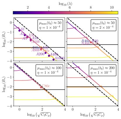
Figure 1: Dependence of the maximum magnetic field strength that can result from a chiral magnetic wave, $B_{*}$ as given by Eq. (20), on the coupling constants $C_{5}$ and $C_{\mu}$. The different panels indicate different combinations of the initial value of the maximum chemical potential, $\mu_{\mathrm{max}}(t_{0})$, and the magnetic resistivity, $\eta$. Colors indicate the value of the feedback parameter $\lambda$. The horizontal black lines indicate the approximate threshold for the production of turbulence, as estimated in Eq. (25), and the dashed black line shows the approximate minimum value above which the velocity of the CMW becomes supersonic, see Appendix A. Overplotted are the values obtained according to Eq. (20) for all the runs presented in this paper; see Tab. 1.

Table 1: Summary of the simulations. The three reference runs are in bold. Runs $A3$ and $A10b$ have been presented also in Schober et al. [56], where they were named $R1$ and $R2$, respectively. Run $R$–$2$ is a comparison run without the CSE, which has been presented in Schober et al. [50].

	Parameters					Initial conditions			Phenomenology			DNS results (maximum values)
Run	Res.	$B_{\mathrm{ex}}$	$\eta$	$\lambda$	$C_{5}=C_{\mu}$	$\mu_{\mathrm{max}}$	$E_{\mu}$	$E_{5}$	$\frac{P_{\mathrm{CMW}}/2}{t_{\mathrm{D}}}$	$B_{*}$	$B_{\mathrm{crit}}$	$\mu_{\mathrm{5,max}}$	$B_{\mathrm{rms}}$	${\rm Re}_{{}_{\mathrm{M}}}$	$\mathrm{Lu}$
$A1$	$672^{3}$	$1\times 10^{-4}$	$1\times 10^{-4}$	$4\times 10^{2}$	$1$	$45$	$\propto k^{-4}$	0	$1400.99$	$0.14$	$0.0022$	$59$	$0.041$	$58$	$200$
$A3$	$1024^{3}$	$1\times 10^{-4}$	$1\times 10^{-4}$	$4\times 10^{2}$	$3$	$45$	$\propto k^{-4}$	0	$467.63$	$0.047$	$0.0023$	$68$	$0.12$	$77$	$440$
$\boldsymbol{A5}$	$\boldsymbol{1024^{3}}$	$\boldsymbol{1\times 10^{-4}}$	$\boldsymbol{1\times 10^{-4}}$	$\boldsymbol{4\times 10^{2}}$	$\boldsymbol{5}$	$\boldsymbol{45}$	$\boldsymbol{\propto k^{-4}}$	$\boldsymbol{0}$	$\boldsymbol{280.60}$	$\boldsymbol{0.028}$	$\boldsymbol{0.0023}$	$\boldsymbol{63}$	$\boldsymbol{0.15}$	$\boldsymbol{110}$	$\boldsymbol{610}$
$A5b$	$720^{3}$	$1\times 10^{-4}$	$1\times 10^{-4}$	$4\times 10^{4}$	$5$	$48$	$\propto k^{-4}$	0	$338.65$	$0.034$	$0.0024$	$50$	$0.011$	$8.4$	$40$
$A10$	$720^{3}$	$1\times 10^{-4}$	$1\times 10^{-4}$	$4\times 10^{2}$	$10$	$48$	$\propto k^{-4}$	0	$169.32$	$0.017$	$0.0024$	$42$	$0.0077$	$0.89$	$9.3$
$A10b$	$672^{3}$	$1\times 10^{-4}$	$1\times 10^{-4}$	$4\times 10^{4}$	$10$	$44$	$\propto k^{-4}$	0	$133.03$	$0.013$	$0.0022$	$38$	$0.024$	$36$	$98$
$A80a$	$448^{3}$	$1\times 10^{-4}$	$1\times 10^{-4}$	$4$	$80$	$44$	$\propto k^{-4}$	0	$17.17$	$0.0017$	$0.0022$	$66$	$0.00043$	$0.054$	$0.45$
$\boldsymbol{A80}$	$\boldsymbol{448^{3}}$	$\boldsymbol{1\times 10^{-4}}$	$\boldsymbol{1\times 10^{-4}}$	$\boldsymbol{4\times 10^{2}}$	$\boldsymbol{80}$	$\boldsymbol{44}$	$\boldsymbol{\propto k^{-4}}$	$\boldsymbol{0}$	$\boldsymbol{17.17}$	$\boldsymbol{0.0017}$	$\boldsymbol{0.0022}$	$\boldsymbol{66}$	$\boldsymbol{0.00043}$	$\boldsymbol{0.054}$	$\boldsymbol{0.45}$
$A80b$	$448^{3}$	$1\times 10^{-4}$	$1\times 10^{-4}$	$4\times 10^{4}$	$80$	$44$	$\propto k^{-4}$	0	$17.17$	$0.0017$	$0.0022$	$66$	$0.00043$	$0.055$	$0.45$
$A80c$	$432^{3}$	$1\times 10^{-4}$	$1\times 10^{-4}$	$4\times 10^{6}$	$80$	$41$	$\propto k^{-4}$	0	$15.00$	$0.0015$	$0.0021$	$38$	$0.00014$	$0.0077$	$0.47$
$A80d$	$432^{3}$	$1\times 10^{-4}$	$1\times 10^{-4}$	$4\times 10^{10}$	$80$	$41$	$\propto k^{-4}$	0	$-$	$0.00018$	$0.0021$	$6.3$	$0.0001$	$0.0039$	$0.6$
$A200$	$448^{3}$	$4\times 10^{-4}$	$1\times 10^{-4}$	$4\times 10^{2}$	$2\times 10^{2}$	$44$	$\propto k^{-4}$	0	$1.70$	$0.00068$	$0.0022$	$65$	$0.00044$	$0.023$	$2.2$
$A400$	$448^{3}$	$4\times 10^{-4}$	$1\times 10^{-4}$	$4\times 10^{2}$	$4\times 10^{2}$	$44$	$\propto k^{-4}$	0	$0.85$	$0.00034$	$0.0022$	$74$	$0.00042$	$0.015$	$1.5$
$\boldsymbol{A1000}$	$\boldsymbol{448^{3}}$	$\boldsymbol{4\times 10^{-4}}$	$\boldsymbol{1\times 10^{-4}}$	$\boldsymbol{4\times 10^{2}}$	$\boldsymbol{1\times 10^{3}}$	$\boldsymbol{44}$	$\boldsymbol{\propto k^{-4}}$	$\boldsymbol{0}$	$\boldsymbol{0.35}$	$\boldsymbol{0.00014}$	$\boldsymbol{0.0022}$	$\boldsymbol{94}$	$\boldsymbol{0.00041}$	$\boldsymbol{0.0039}$	$\boldsymbol{2.2}$
$B40a$	$720^{3}$	$1\times 10^{-4}$	$2\times 10^{-4}$	$4$	$40$	$48$	$\propto k^{-4}$	0	$84.77$	$0.0085$	$0.0048$	$45$	$0.0045$	$0.69$	$5$
$B40$	$720^{3}$	$1\times 10^{-4}$	$2\times 10^{-4}$	$4\times 10^{2}$	$40$	$48$	$\propto k^{-4}$	0	$84.70$	$0.0085$	$0.0048$	$45$	$0.0044$	$0.68$	$4.8$
$B40b$	$720^{3}$	$1\times 10^{-4}$	$2\times 10^{-4}$	$4\times 10^{4}$	$40$	$48$	$\propto k^{-4}$	0	$84.70$	$0.0085$	$0.0048$	$45$	$0.0037$	$0.61$	$4$
$B40c$	$720^{3}$	$1\times 10^{-4}$	$2\times 10^{-4}$	$4\times 10^{6}$	$40$	$48$	$\propto k^{-4}$	0	$84.77$	$0.0085$	$0.0048$	$41$	$0.001$	$0.17$	$0.92$
$B40d$	$720^{3}$	$1\times 10^{-4}$	$2\times 10^{-4}$	$4\times 10^{8}$	$40$	$48$	$\propto k^{-4}$	0	$85.15$	$0.0022$	$0.0048$	$30$	$0.00027$	$0.016$	$0.3$
$C80c$	$720^{3}$	$1\times 10^{-4}$	$1\times 10^{-4}$	$4\times 10^{6}$	$80$	$96$	$\propto k^{-4}$	0	$84.88$	$0.0085$	$0.0048$	$90$	$0.0015$	$0.24$	$1.2$
$R$–$2$	$672^{3}$	$0$	$2\times 10^{-4}$	$4\times 10^{2}$	$0$	$-$	0	$\propto k^{-2}$	$-$	$-$	$-$	$50$	$0.18$	$140$	$460$

Within one period of the wave, $2\pi/\omega_{\mathrm{CMW}}$, the sign of the produced $\mu_{5}$ oscillates between positive and negative. Therefore a chiral dynamo instability can amplify the magnetic field significantly as long as the timescale on which $\mu_{5}$ changes sign,

$$t_{\mathrm{CMW,nl}} \approx \frac{\pi}{\left[C_{5}\,C_{\mu}(k_{\mu,\mathrm{eff}}B_{\mathrm{rms}})^{2}-{1\over 4}(\lambda\eta B_{\mathrm{rms}}^{2})^{2}\right]^{1/2}},\;\;$$ (19)

is longer than the dynamo timescale in Eq. (18). In Eq. (19), we assume that the system is at a stage where magnetic fluctuations are larger than the imposed field. With increasing $B_{\mathrm{rms}}$, $t_{\mathrm{CMW,nl}}$ decreases and eventually becomes comparable with $t_{\mathrm{D}}$. This allows estimating the maximum strength of a magnetic field produced by CMWs. Comparing Eqs. (19) and (18) yields a maximum magnetic field strength of

$$|B_{*}| = \frac{\sqrt{2}}{\eta\lambda}\sqrt{C_{5}\,C_{\mu}}k_{\mu,\mathrm{eff}}\biggl{[}\pm\left(1-\xi^{2}\right)^{1/2}+1\biggr{]}^{1/2}$$ (20)

with

$$\xi\equiv\frac{\pi\lambda\eta^{2}\mu^{2}_{\mathrm{max}}(t_{0})}{4C_{5}\,C_{\mu}k_{\mu,\mathrm{eff}}^{2}}$$ (21)

and where we used the frequency of the CMW as given in Eq. (6). This expression for $B_{*}$ is based on the assumptions that (i) a complete conversion of $\mu$ to $\mu_{5}$ is possible and (ii) that there is no turbulence in the system. It is worth noting that Eq. (20) approaches

$$|B^{-}_{*}| = \frac{\pi\eta\mu^{2}_{\mathrm{max}}(t_{0})}{4\sqrt{C_{5}\,C_{\mu}}k_{\mu,\mathrm{eff}}},$$ (22)

or

$$|B^{+}_{*}| = \frac{2\sqrt{C_{5}\,C_{\mu}}k_{\mu,\mathrm{eff}}}{\eta\lambda},$$ (23)

if $\xi\ll 1$. The physically relevant value is $|B_{*}|=\mathrm{min}(|B^{-}_{*}|,|B^{+}_{*}|)$, because as soon as the magnetic field strength reaches the lower branch of the solutions, the sign of $\mu_{5}$ changes on a timescale that is shorter than $t_{\mathrm{D}}$. In the limit of $\xi\gg 1$ Eq. (20) becomes

$$|B_{*}|=\frac{\sqrt{\pi}}{2\sqrt{\lambda}}~{}\mu_{\mathrm{max}}(t_{0}).$$ (24)

However, in this limit the damping of the CMW can be significant, see Eq. (8), and $\mu_{5,\mathrm{max}}$ never reaches the maximum possible value of $\mu_{5,\mathrm{max}}=\mu_{\mathrm{max}}(t_{0})$. Therefore, the expression in Eq. (24) can be considered as an upper limit. The expression given by Eq. (20) is plotted for different parameters in Fig. 1.

III.5 Production of turbulence and mean-field dynamo instability

Magnetic fluctuations generated by the chiral dynamo instability, produce velocity fluctuations $U_{\mathrm{rms}}$ through the Lorentz force. This leads to an increase of the Reynolds number $\mathrm{Re}_{\mathrm{M}}=U_{\mathrm{rms}}/(k_{\mathrm{f}}\eta)$, where $k_{\mathrm{f}}$ is the forcing wave number. In such magnetically-driven turbulence, $k_{\mathrm{f}}$ is roughly equal to the wavenumber on which the magnetic energy peaks. For a chiral dynamo instability, this corresponds to $k_{\mathrm{f}}\approx k_{\mathrm{5}}=\mu_{5,\mathrm{max}}/2$. Using the rough assumption that $\sqrt{\langle{\rho}\rangle}\,U_{\mathrm{rms}}\approx B_{\mathrm{rms}}$, we can estimate the critical magnetic field strength $B_{\mathrm{crit}}$ which is necessary for the production of turbulence, i.e. for reaching a value of $\mathrm{Re}_{\mathrm{M}}$ above unity. We find that the critical magnetic field strength is estimated as

$$B_{\mathrm{crit}}\approx\sqrt{\langle{\rho}\rangle}\,\eta\frac{\mu_{\mathrm{max}}(t_{0})}{2}.$$ (25)

The value of $B_{\mathrm{crit}}$ is presented as horizontal black lines in Fig. 1. It can be used to illustrate the regions of the parameter regime in which turbulence can be produced.

If the small-scale chiral dynamo leads to a magnetic field that exceeds $B_{\mathrm{crit}}$, a mean-field dynamo instability can be excited. The maximum growth rate of the mean-field dynamo is

$$\gamma_{\alpha}=\frac{(\eta\langle{\mu_{5}}\rangle+\alpha_{\mathrm{M}})^{2}}{4(\eta+\eta_{\mathrm{T}})},$$ (26)

where $\langle{\mu_{5}}\rangle$ is the mean chiral chemical potential and $\alpha_{\mathrm{M}}$ is the magnetic $\alpha$ effect [49, 50]. Here $\alpha_{\mathrm{M}}=2(q-1)/(q+1)\,\tau_{\rm c}\,\chi_{\rm c}/\langle{\rho}\rangle$ is the magnetic $\alpha$ effect, which is determined by the current helicity $\chi_{\rm c}=\langle{\bm{b}}{\bm{\cdot}}({\bm{\nabla}}\times{\bm{b}})\rangle\approx\langle{\bm{a}}\cdot{\bm{b}}\rangle\,k_{\mathrm{f}}^{2}$, where $q$ is the exponent of the magnetic energy spectrum $E_{\rm M}\propto k^{-q}$, and ${\bm{a}}$ and ${\bm{b}}$ are the fluctuations of the vector potential and the magnetic field, respectively. The correlation time of the magnetically-driven turbulence is $\tau_{\rm c}\approx(U_{\mathrm{A}}k_{\mathrm{f}})^{-1}$, where the Alfvén speed is $U_{\rm A}=\sqrt{\langle{\bm{b}}^{2}\rangle}/\sqrt{\langle{\rho}\rangle}\approx B_{\mathrm{rms}}/\sqrt{\langle{\rho}\rangle}$. The turbulent diffusion coefficient $\eta_{\mathrm{T}}$ is estimated as $\eta_{\mathrm{T}}=U_{\mathrm{rms}}/(3k_{\mathrm{f}})$. The characteristic wavenumber on which the mean-field dynamo occurs is

$$k_{\alpha}=\frac{|\eta\langle{\mu_{5}}\rangle+\alpha_{\mathrm{M}}|}{2(\eta+\eta_{\mathrm{T}})}.$$ (27)

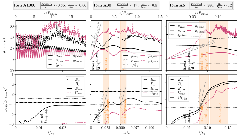
Figure 2: Exemplary runs from the three different regimes: A high-frequency CMW with just chiral tangling (Run $A1000$, left panels), inefficient small-scale chiral dynamo due to a CMW with moderate frequency (Run $A80$, middle panels), and a low-frequency CMW with a small-scale chiral and mean-field dynamo (Run $A5$, right panels). The top panels show the time evolution of the rms and maximum values of the chemical potential $\mu$ and the chiral chemical potential $\mu_{5}$, respectively, as well as the volume average of $\mu$. The bottom panels show the evolution of the rms values of the magnetic and the velocity fields, $B_{\mathrm{rms}}$ and $U_{\mathrm{rms}}$ as well as the external field strength $B_{\mathrm{ex}}$ and the maximum possible magnetic field strength $B_{*}$ if no turbulence is produced. For Run $A5$ the time evolution of the mean magnetic field strength $\langle B\rangle_{\mathrm{int}}$ is presented for comparison.

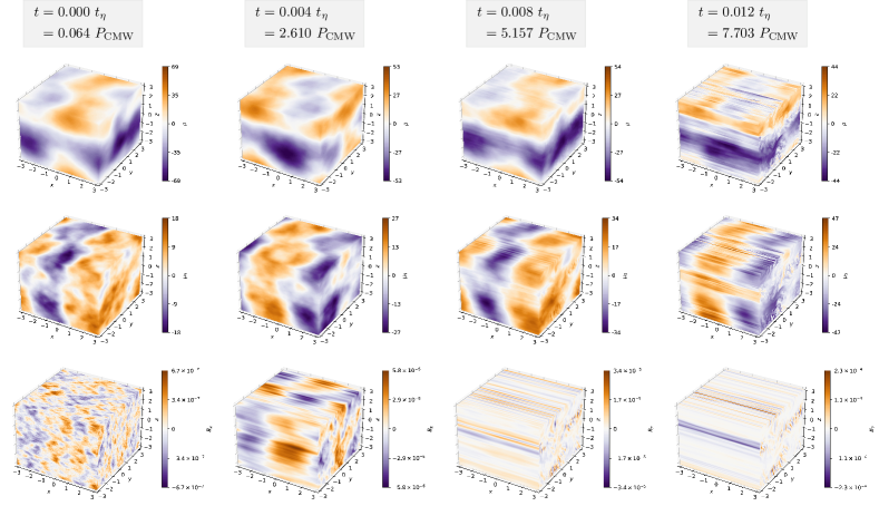
Figure 3: Snapshots of Run $A1000$. The surface of the cubic domain is shown for $\mu$ (upper row), $\mu_{5}$ (middle row), and the $x$ component of the magnetic field $B_{z}$ (lower row). The snapshots cover the different evolutionary phases, from the initial $\mu_{5}$ production phase ($t=0.05~{}t_{\eta}$, first column), to the onset of the chiral dynamo instability ($t=0.10~{}t_{\eta}$, second column), to the early mean-field dynamo stage ($t=0.15~{}t_{\eta}$, third column), and the end of the mean-field dynamo stage ($t=0.20~{}t_{\eta}$, forth column).

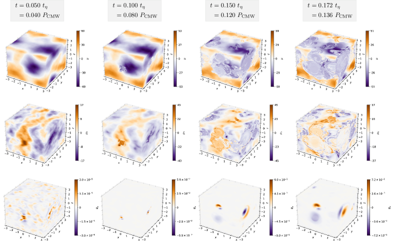
Figure 4: Similar to Fig. 4 but for Run $A5$.

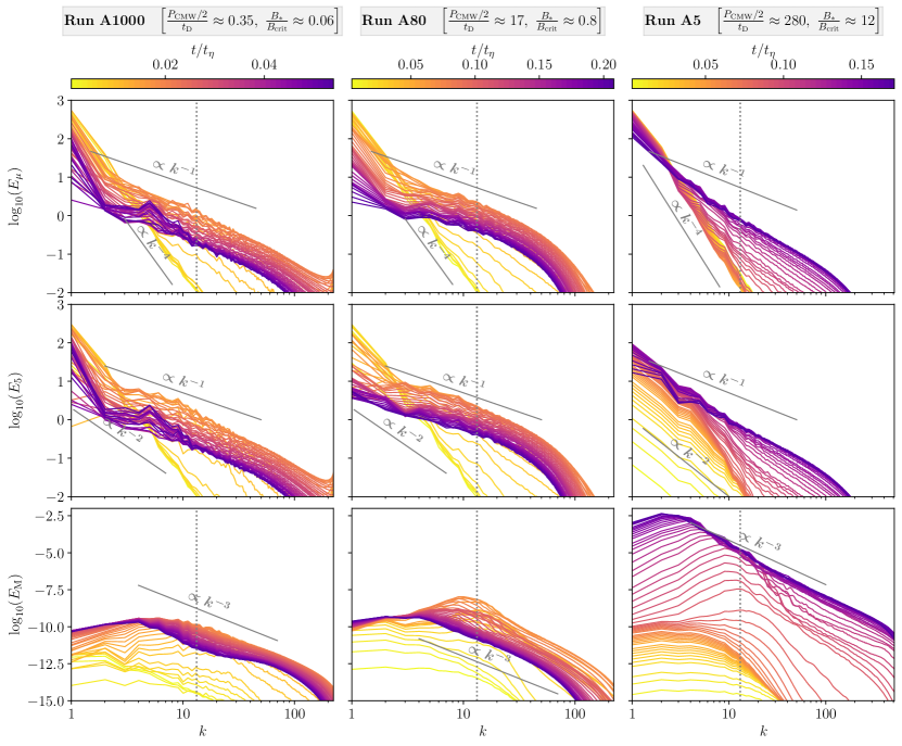
Figure 5: Exemplary runs from the three different regimes: A high-frequency CMW with just chiral tangling (Run $A1000$, left panels), inefficient small-scale chiral dynamo due to a CMW with moderate frequency (Run $A80$, middle panels), and a low-frequency CMW with small-scale chiral and mean-field dynamos (Run $A5$, right panels). From top to bottom, the spectrum of fluctuations of chemical potential, $E_{\mu}(k)$, chiral chemical potential, $E_{5}(k)$, and the magnetic energy spectrum $E_{\mathrm{M}}(k)$ are shown. The vertical dotted line indicates the highest possible value of the small-scale dynamo instability scale, $\mu_{\mathrm{max}}(t_{0})/2$, on which the magnetic field is amplified if all of the initial $\mu$ has been converted to $\mu_{5}$.

IV Numerical simulations

In this section, we use simulations to verify the phenomenology discussed above. Using direct numerical simulations (DNS), the conditions for chiral dynamo instabilities, efficient magnetic field amplification and, in particular, the mean-field dynamo phase can be analyzed qualitatively.

IV.1 Setup and analysis tools

We use the Pencil Code [57] to solve equations (1)–(5) in a three-dimensional periodic domain of size $L^{3}=(2\pi)^{3}$ with a resolution of up to $1024^{3}$. This code employs a third-order accurate time-stepping method [58] and sixth-order explicit finite differences in space [59, 60]. The smallest wave number covered in the numerical domain is $k_{1}=2\pi/L=1$ which we use for normalization of length scales. All velocities are normalized to the sound speed $c_{\rm s}=1$ and the mean fluid density is set to $\langle{\rho}\rangle=1$. Further, the magnetic Prandtl number is $1$, i.e. the magnetic diffusivity equals the viscosity. Time is normalized either by the diffusion time $t_{\eta}=(\eta k_{1}^{2})^{-1}$ or by the period of the chiral magnetic wave $P_{\mathrm{CMW}}$.

The simulation parameters have been selected to cover the three different regimes: the “chiral tangling regime” ($t_{\mathrm{D}}\gtrsim P_{\mathrm{CMW}}/2$), the “small-scale chiral dynamo regime” ($t_{\mathrm{D}}\lesssim P_{\mathrm{CMW}}/2$ and $B_{*}\lesssim B_{\mathrm{crit}}$) and the “mean-field dynamo regime” ($t_{\mathrm{D}}\lesssim P_{\mathrm{CMW}}/2$ and $B_{*}\gtrsim B_{\mathrm{crit}}$). We also perform a comparison with the results obtained in our previous study Ref. [49] (see Run $R$–$2$ there), where chiral dynamo instabilities were found for an initial $\mu_{5}\not=0$ with zero mean but spatial fluctuations. For this comparison, the spatial maximum value of the chemical potential at the initial time $t_{0}$, $\mu_{\mathrm{max}}$, and its spectrum $E_{\mu}(k,t_{0})$ have been chosen to eventually (before the onset of the small-scale chiral instability) result in a state of the system that is comparable to the initial conditions in the Run $R$–$2$. In particular, in the Run $R$–$2$ the initial $\mu_{5,\mathrm{max}}$ was $\approx 50$ and the initial spectrum was $E_{5}(k,t_{0})\propto k^{-2}$. We therefore choose, for most runs of this study, $\mu_{\mathrm{max}}(t_{0})\approx 50$ and $E_{\mu}(k,t_{0})\propto k^{-4}$ which results in the spectrum $E_{5}(k,t_{0})\propto k^{-2}$ according to Eq. (13).

The range of parameters chosen for this study is also based on numerical aspects. The parameter space that we explore includes the regime where the magnetic field strength becomes larger than the critical value $B_{\mathrm{crit}}$ for the production of turbulence and the subsequent excitation of mean-field dynamos. According to the estimate in Eq. (20), which is illustrated in Fig. 1, the maximum magnetic field strength $B_{*}$ is higher for lower frequencies $\omega_{\mathrm{CMW}}$ of the CMW. However, for low $\omega_{\mathrm{CMW}}$ and therefore low values of $C_{5}$, the initial linear production of $\mu_{5}$ becomes very slow, as can be seen in Eq. (10). Increasing the initial value of $\mu$ increases the initial production rate of $\mu_{5}$, but this also leads to a larger value $B_{*}$, which can cause the characteristic velocity of the CMW to become comparable or larger than the sound speed. Additionally, larger values of the initial $\mu$ lead to larger values of $\mu_{5}$ and therefore a higher characteristic wave number of the chiral dynamo instability. Hence sufficient spatial resolution is required. More details on the numerical criteria are given in Appendix A.

Due to the numerical constraints discussed above, and also to allow for an appropriate comparison with the DNSs presented in [49, 50], we initiate most of the simulations with $\mu_{\mathrm{max}}(t_{0})\approx 50$ and use $\eta=10^{-4}$. We name this main series of simulations Series A. Series B has $\mu_{\mathrm{max}}(t_{0})\approx 50$ and $\eta=2\times 10^{-4}$ and Series C has $\mu_{\mathrm{max}}(t_{0})\approx 100$ and $\eta=10^{-4}$. A summary of all runs of this study is given in Table 1 and the values for the corresponding estimates of $B_{*}$ is shown in Fig. 1. Comparing the estimates $B_{*}$ and $B_{\mathrm{crit}}$, we can expect the occurrence of turbulence in Runs $A1$, $A3$, $A5$, $A5b$, and potentially in Runs $A10$ and $A10b$. All other runs are expected to result in values of $B_{*}$ that are comparable or below $B_{\mathrm{crit}}$.

For runs in which turbulence develops, we perform a mean-field analysis. To this end, an averaging of the instantaneous fields needs to be performed in the DNS. Since turbulence is driven magnetically, the forcing scale $k_{f}$ corresponds to the integral scale of the magnetic field which we determine via the magnetic energy spectrum $E_{\mathrm{M}}(k)$ as

$$k_{\mathrm{int}}\equiv\left[\frac{1}{{\cal E}_{\rm M}}\int E_{\mathrm{M}}(k)\,k^{-1}~{}\mathrm{d}k\right]^{-1}.$$ (28)

Magnetic energy density ${\cal E}_{\rm M}$ and magnetic spectrum $E_{\mathrm{M}}(k)$ are connected as

$${\cal E}_{\rm M}\equiv\frac{B_{\mathrm{rms}}^{2}}{2}=\int E_{\mathrm{M}}(k)\,\mathrm{d}k.$$ (29)

To take into account that the magnetically-driven turbulence exists in the range of the wave numbers $k\geq k_{\mathrm{int}}$, we define the mean quantity $X$ in simulations as

$$\langle X\rangle_{\mathrm{int}}\equiv\left[\int E_{\mathrm{X}}(k)f(k)\,\mathrm{d}k\right]^{1/2},$$ (30)

where we use the function

$$f(k)\equiv\left[1-\mathrm{tanh}(k-k_{\mathrm{int}})\right]/2$$ (31)

to filter out the scale $k\gtrsim k_{\mathrm{int}}$. The result of taking the average $\langle X\rangle_{\mathrm{int}}$ is typically different from the volume average, which is denoted by $\langle X\rangle_{\mathrm{V}}$.

IV.2 Results for the reference runs

In this section, we present three reference runs that have the same initial chemical potential, but different frequencies of the CMW. Run $A1000$ is the run in our sample with the highest frequency of the CMW. With a ratio of $P_{\mathrm{CMW}}/(2t_{\mathrm{D}})\approx 0.35$, no dynamo activity is expected in Run $A1000$. The second reference run is $A80$, which has $P_{\mathrm{CMW}}/(2t_{\mathrm{D}})\approx 17$. Therefore, a small-scale chiral dynamo can occur. However since the expected maximum magnetic field strength $B_{*}\approx 0.0017$ is lower than the critical value $B_{\mathrm{crit}}\approx 0.0017$ that is necessary for the production of turbulence, no mean-field dynamo is expected in Run $A80$. A mean-field dynamo can occur in the third reference run, Run $A5$, which has $B_{*}/B_{\mathrm{crit}}\approx 12$. Run $A5$ is the run with the third to the highest value of $P_{\mathrm{CMW}}/(2t_{\mathrm{D}})$ in our sample. We discuss the results of the reference runs in the following and confront them with the estimates based on the phenomenological estimates presented in Sec. III.

The left panels of Fig. 2 show the time evolution of various parameters of Run $A1000$. In the top left panel, the oscillatory behavior of $\mu_{\mathrm{rms}}$ and $\mu_{5,\mathrm{rms}}$ is clearly seen and the time evolution governs almost $20$ periods of the CMW. In systems like this, where the CMW has a very high frequency and the initial chiral chemical potential is small, the timescale of the chiral dynamo $t_{\mathrm{D}}$ is much longer than $P_{\mathrm{CMW}}$. In this case, magnetic fluctuations can only be amplified by chiral tangling. This phenomenon alone leads to the production of magnetic fluctuations that are of the order of the imposed magnetic field $B_{\mathrm{ex}}$. The magnetic field evolution in Run $A1000$ can be seen in the lower left panel of Fig. 2. The maximum value of $B_{\mathrm{rms}}$ produced by chiral tangling alone is approximately less than half of $B_{\mathrm{ex}}$. At $t\gtrsim 0.02~{}t_{\eta}$, both $\mu_{\mathrm{rms}}$ and $\mu_{5,\mathrm{rms}}$ decay, and therefore $B_{\mathrm{rms}}$ decreases.

Snapshots of Run $A1000$ are presented in Fig. 3. While the magnetic field is, as in all simulations of this paper, set up as weak and random fluctuations, the magnetic fluctuations quickly develop into patches that are stretched along the $x$ axis. At the forth snapshot shown here (at $t\approx 7.7~{}P_{\mathrm{CMW}}$), the $B_{x}$ patches stretch out through the entire numerical domain. The magnetic field structure produced by chiral tangling is therefore very different from what is expected when a small-scale chiral dynamo instability is excited. In linear theory, the magnetic field instability is expected to occur on a characteristic wavenumber that is half of the value of $\mu_{5,\mathrm{max}}$. This leads to the formation of isotropic patches of high absolute values of $B_{x}$ on the surface of the numerical domain, at the locations where $\mu_{5}$ reaches the maximum value.

The middle panels of Fig. 2 show the time evolution of various parameters of Run $A80$, where a small-scale chiral dynamo instability occurs. Two oscillations between $\mu_{\mathrm{rms}}$ and $\mu_{5,\mathrm{rms}}$ are seen in the upper middle panel. The initial production of the spatial maximum value of $\mu_{5}(t)$, $\mu_{5,\mathrm{max}}(t)$, proceeds linear in time and follows the prediction given by Eq. (10) until the instant $t\approx 0.015\,t_{\eta}$. Temporal maxima of $\mu_{5,\mathrm{rms}}$ are reached at $t\approx 0.025\,t_{\eta}$ and $t\approx 0.055\,t_{\eta}$. These times coincide, as expected, with an increased growth rate of the magnetic field; see the time evolution of magnetic fluctuations in the lower middle panel. However, the magnetic field fluctuations, $B_{\mathrm{rms}}$, never reach a field strength that is much larger than the one of the imposed field $B_{\mathrm{ex}}$. At its maximum, the rms magnetic field strength is approximately $0.2~{}B_{*}$ in Run $A80$. At later times, $t\gtrsim 1.0\,P_{\mathrm{CMW}}$, the quantities $\mu_{\mathrm{rms}}$, $\mu_{5,\mathrm{rms}}$, and $B_{\mathrm{rms}}$ decay.

The estimated maximum value of $B_{\mathrm{rms}}$, $B_{*}$, is $16$ times higher in Run $A5$ than in $A80$. Contrary to the other reference runs, in Run $A5$, the maximum value $B_{*}$ of magnetic field exceeds $B_{\mathrm{crit}}$, which implies that turbulence can be produced. The time evolution of Run $A5$ is shown in the right panels of Fig. 2. Due to the smaller value of $\omega_{\mathrm{CMW}}$, the production of $\mu_{5}$ is much slower than that in Run $A80$. Here, the threshold for the small-scale chiral dynamo instability only being exceeded at $t\approx 0.08\,t_{\eta}$. After the magnetic field has been amplified by more than two orders of magnitude through the small-scale chiral dynamo, a mean-field dynamo instability is excited at $t\approx 0.11~{}t_{\eta}$ with a growth rate of the magnetic field that is less than that for the small-scale chiral dynamo instability. In Run $A5$, the magnetic field strength exceeds $B_{*}$ by a factor of $\approx 5.4$. The analysis of the mean-field dynamo phase of Run $A5$ and the other runs in which the value of the Reynolds number eventually exceeds unity will be discussed in more detail in Sec. IV.4.

The time evolution of the simulation snapshots for Run $A5$ is presented in Fig. 4. Here, the values for the quantities $\mu$, $\mu_{5}$, and the $x$ component of the magnetic field, $B_{x}$, on the surface of the cubic domain are shown for $t=0.05~{}t_{\eta}-0.172~{}t_{\eta}$. The snapshots show that, as expected, $\mu_{5}$ grows fastest where the gradient of $\mu$ is largest. At $t=0.05~{}t_{\eta}$, the fastest production of $\mu_{5}$ occurs approximately in the middle of the front $x$-$z$ plane (where $\mu_{5}$ is produced with a positive sign) and in the middle of the front of the $x$-$y$ plane (where $\mu_{5}$ is produced with a negative sign). These are the two locations on the shown surface of the domain, where also the magnetic field instability kicks in the fastest.

In the snapshot at time $t=0.10~{}t_{\eta}$, the magnetic field grows approximately on the length scale $k_{5}^{-1}\approx(\mu_{5}/2)^{-1}\approx 1/20$. At $t=0.20~{}t_{\eta}$, the simulation is at the end of the mean-field dynamo stage and the characteristic length scale of the magnetic field has increased. At late times, we also observe that both $\mu$ and $\mu_{5}$ develop small-scale fluctuations, especially in locations where the magnetic field is the strongest. These small-scale structures are symmetric in $\mu$ and $\mu_{5}$, but with opposite sign.

For a quantitative analysis of the evolution of the characteristic scales, the evolution of the energy spectra is presented in Fig. 5 for Runs $A1000$ (middle panels), $A80$ (middle panels), and $A5$ (right panels). In all cases, the initial spectrum of $\mu_{5}$, $E_{5}(k)$, scales with the wave number as $k^{-2}$, as expected for an initial $E_{\mu}(k)$ spectrum that is proportional to $k^{-4}$; see Eq. (13). For Runs $A1000$ $A80$, the initial $k^{-2}$ scaling of $E_{5}(k)$ is less visible due to the fast production of $\mu_{5}$. At later times, the spectra $E_{5}(k)$ and $E_{\mu}(k)$, approach a scaling of $k^{-1}$, as has been reported in [49]. The evolution of the magnetic energy spectra $E_{\mathrm{M}}(k)$ is shown in the lowest panels of Fig. 5. In the case of Run $A80$, a short phase of amplification on $k=\mu_{\mathrm{max}}(t_{0})/2\approx 22$ is seen, but at $t\gtrsim 0.07\,t_{\eta}$ the magnetic energy decays and a $E_{\mathrm{M}}\propto k^{-3}$ develops. The magnetic field amplification is much more efficient in Run $A5$. Here the initial instability occurs also on $k=\mu(t_{0})\approx 22$. Due to the production of turbulence, however, the peak of the magnetic energy spectrum moves to smaller wave numbers. Eventually, a $E_{\mathrm{M}}\propto k^{-3}$ develops in Run $A5$ as well.

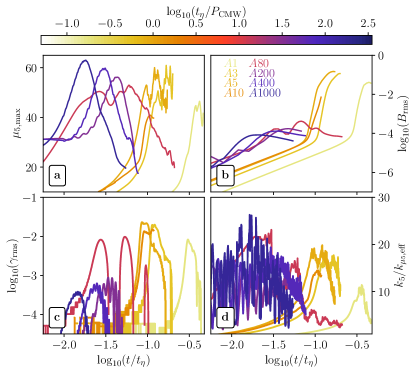
Figure 6: Time series for runs with different values of the ratio of the CMW period over the resistive time, $P_{\mathrm{CMW}}/t_{\eta}$, as indicated by the colorbar. (a) Maximum values of chemical and chiral chemical potential, $\mu_{5,\mathrm{max}}$ and $\mu_{\mathrm{max}}$. (b) Rms value of the magnetic field strength $B_{\mathrm{rms}}$. (c) Measured growth rate $\gamma_{\mathrm{rms}}$ of $B_{\mathrm{rms}}$. (d) The measured scale separation $k_{5}/k_{\mu_{5},\mathrm{eff}}$.

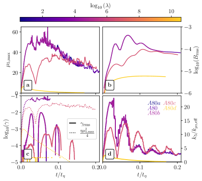
Figure 7: Time series for runs with different values of $\lambda$, as indicated by the colorbar. (a) Maximum values of chemical and chiral chemical potential, $\mu_{5,\mathrm{max}}$ and $\mu_{\mathrm{max}}$. (b) Rms value of the magnetic field strength $B_{\mathrm{rms}}$. (c) Measured growth rate $\gamma_{\mathrm{rms}}$ of $B_{\mathrm{rms}}$, and the theoretical value $\eta\mu_{5,\mathrm{max}}^{2}/4$ of the maximum growth rate, which would be reached for an infinite scale separation ($k_{5}\gg k_{\mu_{5},\mathrm{eff}}$). (d) The measured scale separation $k_{5}/k_{\mu_{5},\mathrm{eff}}$.

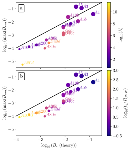
Figure 8: The maximum value of $B_{\mathrm{rms}}$ measured in all runs as a function of the phenomenologically derived maximum, $B_{*}$. Colors indicate (a) the value of $\lambda$ and (b) the ratio of the resistive time $t_{\eta}$ over the period $P_{\mathrm{CMW}}$ of the CMW [Note, that Run $A80d$ is not shown in panel b since there is no CMW]. The size of the symbols increases with increasing maximum Reynolds number obtained in the individual runs.

IV.3 Exploration of the parameter space

A direct comparison between runs with different CMW frequencies $\omega_{\mathrm{CMW}}$, including Runs $A5$, $A80$ and $A1000$, is presented in Fig. 6. All of the runs in Fig. 6 have the same initial values of $\mu$, and the same $\lambda$ and $\eta$. Even though the temporal maximum values of $\mu_{5,\mathrm{max}}$ is higher for runs with higher $\omega_{\mathrm{CMW}}$, the maximum value of the produced magnetic field decreases with increasing $\omega_{\mathrm{CMW}}$. Therefore, CMWs with higher frequencies are less efficient in amplifying the magnetic field. This stems from the small-scale chiral dynamo being less efficient when the period of the CMW is small.

Figure 7 shows a comparison between runs with different chiral feedback parameter, $\lambda$. As expected from Eq. (20), larger values of $\lambda$ lead to lower magnetic field strengths. In Fig 7a, it can be seen that $\mu_{5,\mathrm{max}}$ in all runs with low $\lambda$ reach a value that is comparable to (or even slightly exceeds) the initial value of $\mu_{\mathrm{max}}$. This leads to three instances of magnetic field amplification, see Fig 7b. In Run $A80c$, which has $\lambda=4\times 10^{6}$, lower values of $\mu_{\mathrm{max}}$ are reached, which is caused by the damping of the CMW according to Eq. (8). However, phases of magnetic field amplification can still be seen for Run $A80c$. This is different for Run $A80d$, which has $\lambda=4\times 10^{8}$. Here, no CMW occurs since the frequency of the wave is imaginary.

The maximum magnetic field strength found in DNS agrees well with the prediction given by Eq. (20), as is illustrated in Fig. 8. Here, the predicted value $B_{*}$ is plotted against the temporal maximum of the magnetic field strength in all DNS of this study. The agreement between phenomenology and DNS is better for runs with lower values of $\lambda$. This follows from the fact that Eq. (20) is based on two assumptions: (i) the effective correlation wave number of $\mu$, $k_{\mu,\mathrm{eff}}$, stays constant until the maximum magnetic field strength is reached, and (ii) $\mu_{5,\mathrm{max}}$ can reach the same value as $\mu_{\mathrm{max}}(t_{0})$. As can be seen in Fig 7a, the conversion between $\mu$ and $\mu_{5}$ becomes less efficient when $\lambda$ increases. Even though all runs in Fig. 7 have similar values of $\mu_{\mathrm{max}}(t_{0})\approx 45$, in the run $A80d$ the temporal maximum of $\mu_{\mathrm{5,max}}$ never exceeds $6.3$. Therefore, in the limit of large $\lambda$, the expression in Eq. (20) has to be considered as an upper limit for the maximum possible magnetic field strength.

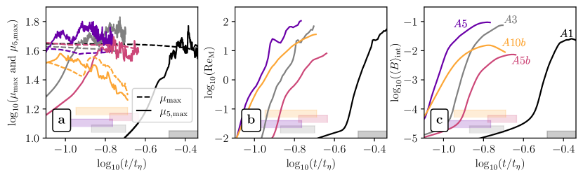
Figure 9: Time evolution of all runs in which magnetically-dominated turbulence is produced. Different colored lines indicate the different runs (A1, A3, A5, A5b, and A10b) as indicated in panel (c). (a) Time evolution of $\mu_{\mathrm{max}}$ (dashed lines) and $\mu_{5,\mathrm{max}}$ (solid lines). (b) Time evolution of the magnetic Reynolds number $\mathrm{Re}_{\mathrm{M}}$. (c) Time evolution of the magnetic field strength $\langle B\rangle_{\mathrm{int}}$ averaged on the integral scale. The color bars in the panels highlight the time range in which the Reynolds number is larger than unity. This time range is shown in Fig. 10.

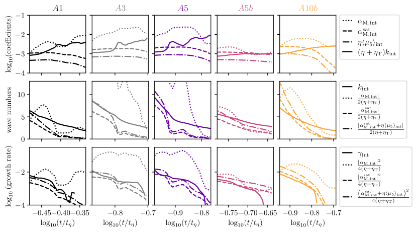
Figure 10: Mean-field dynamo analysis for all runs in which magnetically-dominated turbulence is produced. Different rows of panels indicate the different runs (A1, A3, A5, A5b, and A10b) as indicated on the top. The time axis is reduced to the phase of the DNS, where the Reynolds number is larger than unity up to the final time of the individual simulations. This time range is also indicated by the color blocks in panels (a)-(c) of Fig. 9. (Upper row) Time evolution of dynamo coefficients, $\alpha_{\mathrm{M,int}}$ (dotted lines), $\alpha^{\mathrm{sat}}_{\mathrm{M,int}}$ (dashed lines), and $\eta+\eta_{\mathrm{T}}$ multiplied by the integral wave number $k_{\mathrm{int}}$ (solid lines). The evolution of $\eta\langle\mu_{5}\rangle_{\mathrm{M,int}}$ (dashed-dotted lines) is also shown, which can be relevant for the mean-field dynamo. (Middle row) Time evolution of the integral scale of the magnetic field $k_{\mathrm{int}}$ as measured in the DNS (solid lines). This evolution is compared to theoretical estimates of the mean-field dynamo theory that is based on the turbulent transport coefficients. Different expressions for the magnetic $\alpha$ effect are used: $\alpha_{\mathrm{M,int}}$ (dotted lines) and $\alpha^{\mathrm{sat}}_{\mathrm{M,int}}$ (dashed lines and dashed-dotted lines). (Bottom row) Same as middle row, but for the measured growth rate of $\langle B\rangle_{\mathrm{int}}$ in DNS, $\gamma_{\mathrm{int}}$, and different theoretical estimates.

IV.4 DNS with mean-field dynamo activity

As can be seen in Fig. 8, the maximum magnetic field tends to exceed the estimate from Eq. (20) for runs that develop turbulence. This is understandable, since during the mean-field dynamo phase, the sign of $\mu_{5}$ does not affect the magnetic field amplification. Therefore, the comparison between the timescale of the CMW and the chiral dynamo instability that leads to the estimate given by Eq. (20), is not applicable in the presence of turbulence. The magnetic field can grow to higher strengths, until saturation occurs due to non-linear effects.

In runs with low-frequency CMWs, the magnetic field strength reaches the highest values, leading to efficient driving of magnetically dominated turbulence. In this case, a large-scale magnetic field is generated via a mean-field dynamo instability, as can be seen in the snapshots of Run $A5$ in Fig. 4. Out of all the runs presented here, the ones in which $\mathrm{Re}_{\mathrm{M}}$ exceeds unity, i.e. in which turbulence develops, are Runs $A1$, $A3$, $A5$, $A5b$, and $A10b$. The time series of various quantities of these runs are directly compared in Fig. 9. After the turbulence production phase, the value of $\mu_{5,\mathrm{max}}$ is comparable in Runs $A1$, $A3$, $A5$, and $A5b$. In Run $A10b$, $\mu_{5,\mathrm{max}}$ never exceeds $40$, which is due to the higher frequency of the CMW. In all runs, the magnetic Reynolds number exceeds unity after less than a resistive time; see Fig. 9b. With $\mathrm{Re}_{\mathrm{M}}$ becoming larger than one, the type of dynamo instability changes from a small-scale chiral dynamo to a mean-field dynamo. This transition, which is accompanied by a change in the growth rate, can be seen in Fig. 9c, where the time evolution of the mean magnetic field strength is presented.

The theoretically expected growth rate during the mean-field dynamo phase is given by Eq. (26). In the simulations, we estimate the magnetic $\alpha$ effect as $\alpha_{\mathrm{M,int}}=2(q-1)/(q+1)\,\tau_{\rm c}\,\chi_{\rm c}\approx\tau_{\rm c}\langle{\bm{a}}\cdot{\bm{b}}\rangle_{\mathrm{int}}\,k_{\mathrm{int}}^{2}$, assuming that the forcing scale is $k_{\mathrm{f}}\approx k_{\mathrm{int}}$ and that the exponent of the magnetic energy spectrum $q\approx 3$. The correlation time of the magnetically-driven turbulence is $\tau_{\rm c}\approx(U_{\mathrm{A}}k_{\mathrm{int}})^{-1}$, where the Alfvén speed is $U_{\rm A}=\sqrt{\langle{\bm{b}}^{2}\rangle}\approx B_{\mathrm{rms}}$. The mean fluid density $\langle{\rho}\rangle$ entering in $U_{\rm A}$ and $\alpha_{\mathrm{M}}$ is set to unity in the DNS. The turbulent diffusion coefficient $\eta_{\mathrm{T}}$ is estimated as $\eta_{\mathrm{T}}=U_{\mathrm{rms}}/(3k_{\mathrm{int}})$. The time evolution of $\alpha_{\mathrm{M,int}}$ and $\eta_{\mathrm{T}}$ for all turbulent runs is presented in the upper panels of Fig. 10. The time range shown in Fig. 10 is the moment when $\mathrm{Re}_{\mathrm{M}}$ exceeds unity up to the final time of the simulation, i.e. it governs the turbulent phase of the simulation. Right after the onset of turbulence, $\alpha_{\mathrm{M,int}}$ is the dominant transport coefficient for all runs presented in Fig. 10. However, $\eta_{\mathrm{T}}$ grows constantly with time.

The magnetic $\alpha$ effect can also be estimated from the evolutionary equation for the magnetic helicity $\langle{\bm{a}}\cdot{\bm{b}}\rangle$ of the small-scale field ${\bm{b}}={\bm{\nabla}}\times{\bm{a}}$ in chiral MHD [17]:

$${\partial\over\partial t}\langle{\bm{a}}{\bm{\cdot}}{\bm{b}}\rangle+\nabla\cdot{\bm{F}} = 2\eta\,\langle\mu_{5}\rangle\langle{\bm{b}}^{2}\rangle-2\langle\mbox{\boldmath{${\cal{E}}$}}\rangle{}\cdot\langle\mbox{\boldmath$B$}\rangle{}$$ (32)

$$-2\eta\,\langle{\bm{b}}\,({\bm{\nabla}}\times{\bm{b}})\rangle,$$

where ${\bm{F}}$ is the flux of $\langle{\bm{a}}{\bm{\cdot}}{\bm{b}}\rangle$ that is given by

$${\bm{F}} = \left\langle{\bm{u}}\,a_{j}\right\rangle\left\langle B_{j}\right\rangle-\langle\mbox{\boldmath$B$}\rangle{}\left\langle{\bm{a}}\cdot{\bm{u}}\right\rangle-\eta\left\langle{\bm{a}}\times({\bm{\nabla}}\times{\bm{b}})\right\rangle$$ (33)

$$+\left\langle{\bm{a}}\times({\bm{u}}\times{\bm{b}})\right\rangle,$$

and $\langle\mbox{\boldmath{${\cal{E}}$}}\rangle{}\equiv\langle{\bm{u}}{\bm{\times}}{\bm{b}}\rangle=\alpha_{\mathrm{M}}\langle\mbox{\boldmath$B$}\rangle{}-\eta_{T}\,({\bm{\nabla}}\times\langle\mbox{\boldmath$B$}\rangle{})$ is the turbulent electromotive force. In the steady-state, two leading source/sink terms in Eq. (32), $2\eta\,\langle\mu_{5}\rangle\langle{\bm{b}}^{2}\rangle-2\alpha_{\mathrm{M}}\langle\mbox{\boldmath$B$}\rangle{}^{2}$, compensate each other, so that the magnetic $\alpha$ effect reaches [49, 50]

$$\alpha_{\mathrm{M}}^{\rm sat}=\eta\,\langle\mu_{5}\rangle\,\frac{\langle{\bm{b}}^{2}\rangle}{\langle\mbox{\boldmath$B$}\rangle{}^{2}}.$$ (34)

The time evolution of $\alpha_{\mathrm{M,int}}^{\rm sat}=\eta\langle\mu_{5}\rangle_{\mathrm{int}}B_{\mathrm{rms}}^{2}/\langle B\rangle_{\mathrm{int}}^{2}$ is compared to the one of $\alpha_{\mathrm{M,int}}$ in the upper panels of Fig. 10. We note that the values of $\alpha_{\mathrm{M,int}}^{\rm sat}$ are consistently lower than $\alpha_{\mathrm{M,int}}$, which could result from the fact that the divergence of the magnetic helicity fluxes is ignored in the estimate of $\alpha_{\mathrm{M,int}}^{\rm sat}$.

In the middle and lower panels of Fig. 10, the estimates of the turbulent transport coefficients are used to calculate the theoretically expected characteristic wavenumber $k_{\alpha}$ and growth rate $\gamma_{\alpha}$ of the mean-field dynamo, respectively. The theoretical estimates, given by Eqns. (26) and (27), are compared with the measured characteristic wavenumber of the magnetic field, $k_{\mathrm{int}}$ and the measured growth rate $\gamma_{\mathrm{int}}$ of the mean magnetic field strength $\langle B\rangle_{\mathrm{int}}$. In the middle row of Fig. 10 we compare the measured $k_{\mathrm{int}}$ to $|\alpha_{\mathrm{M,int}}|/\left[2(\eta+\eta_{\mathrm{T}}))\right]$ and $|\alpha_{\mathrm{M,int}}^{\mathrm{sat}}|/\left[2(\eta+\eta_{\mathrm{T}})\right]$, respectively, and in the bottom row, we compare the measured $\gamma_{\mathrm{int}}$ to $|\alpha_{\mathrm{M,int}}|^{2}/\left[4(\eta+\eta_{\mathrm{T}})\right]$ and $|\alpha_{\mathrm{M,int}}^{\mathrm{sat}}|^{2}/\left[4(\eta+\eta_{\mathrm{T}})\right]$, respectively. Using the $\alpha_{\mathrm{M,int}}$ to estimate $k_{\alpha}$ and $\gamma_{\alpha}$, tends to lead to slightly higher values than the measured $k_{\mathrm{int}}$ and $\gamma_{\mathrm{int}}$, while using $\alpha_{\mathrm{M,int}}^{\rm sat}$, leads to slightly lower values.

One issue that arises in the comparison with theory is that while computing the mean value of $\langle\mu_{5}\rangle_{\mathrm{int}}$ the information about the sign is lost, as the averaging process is based on the spectrum of $\mu_{5}^{2}$. This is a problem because the expressions of $k_{\alpha}$ and $\gamma_{\alpha}$, as given in Eqs. (27) and (26), include the sum of $\eta\langle{\mu_{5}}\rangle$ and $\alpha_{\mathrm{M}}$. For strong turbulence, we expect that $\alpha_{\mathrm{M}}\gg\eta\langle{\mu_{5}}\rangle$, and therefore we neglect the $\eta\langle{\mu_{5}}\rangle_{\mathrm{int}}$ term in the estimates. But for systems with low Reynolds numbers, the sign of $\langle\mu_{5}\rangle_{\mathrm{int}}$ can be relevant in the comparison between DNS and mean-field theory. As can be seen in the upper row of Fig. 10, indeed, in our simulations, the contribution of $\eta\langle{\mu_{5}}\rangle_{\mathrm{int}}$ can be relevant as it is not much smaller than the values of $\alpha_{\mathrm{M,int}}$ and $\alpha_{\mathrm{M,int}}^{\mathrm{sat}}$ As $\alpha_{\mathrm{M,int}}^{\rm sat}$ is proportional to $\langle\mu_{5}\rangle_{\mathrm{int}}$, for this case the sign of $\langle\mu_{5}\rangle_{\mathrm{int}}$ is irrelevant in the expression $|\alpha_{\mathrm{M}}+\eta\langle{\mu_{5}}\rangle|$, and we can use the full expressions from Eqs. (27) and (26), which are shown as dashed-dotted lines in the middle and bottom rows of Fig. 10. The contribution of $\eta\langle{\mu_{5}}\rangle$ leads to slightly higher characteristic wavenumbers and growth rates, which generally agree better with the directly measured values of $k_{\mathrm{int}}$ and $\gamma_{\mathrm{int}}$.

All of the turbulent runs presented in Figs. 9 and 10 reach saturation eventually, i.e. the mean magnetic field stops growing. This can be seen in the time evolution of $\langle B\rangle_{\mathrm{int}}$ in Fig. 9 and in the bottom row of Fig. 10, where $\gamma_{\mathrm{int}}$ vanishes towards the end of the individual runs. In case of mean-field dynamos, the maximum magnetic field strength cannot be estimated by $B_{*}$ as given by Eq. 20, because the characteristic timescale are different from that of the small-scale chiral dynamo. Instead, we expect non-linear effects to play a role in the mean-field dynamo saturation. In particular, the growth rate of this dynamo vanishes when $|(\eta+\eta_{\mathrm{T}})k_{\mathrm{int}}|\approx|\alpha_{\mathrm{M}}+\eta\langle{\mu_{5}}\rangle|\approx|\alpha_{\mathrm{M}}|$. Indeed, we find that $(\eta+\eta_{\mathrm{T}})k_{\mathrm{int}}$ becomes comparable to the different estimates of $\alpha_{\mathrm{M}}$ (see the top row of Fig. 10) at the same time when $\gamma_{\mathrm{int}}$ vanishes (see the bottom row of Fig. 10).

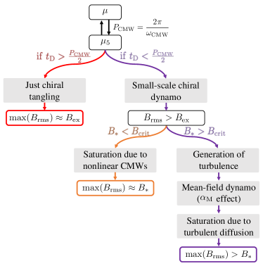
Figure 11: Summary of the three different regimes in systems with vanishing initial chiral asymmetry, in which $\mu_{5}$ is generated through the chiral separation effect. The maximum magnetic field strength is the lowest in the regime where just chiral tangling occurs (left side of the sketch). When the small-scale chiral dynamo instability is excited, the maximum field strength is either given by $B_{*}$ (see Eq. 20; middle part of the sketch) or larger if magnetically-driven turbulence is produced (right side of the sketch).

V Discussion and Conclusions

In this paper, we have studied a high-energy plasma with joint action of the chiral magnetic effect (CME) and the chiral separation effect (CSE). We considered a very weak initial magnetic field in the form of Gaussian fluctuations plus a weak external magnetic field $B_{\mathrm{ex}}$. The initial chiral chemical potential $\mu_{5}$ is zero, but there is a strong initial gradient of the chemical potential fluctuations $\mu$. Through the CSE, chiral magnetic waves (CMWs) generate inhomogeneous fluctuations of $\mu_{5}$. As there is no (initial) velocity field in the system, the only way for the magnetic field to get amplified in this scenario is through the produced chiral asymmetry (i.e., a non-zero $\mu_{5}$). The generation of the magnetic field is caused by the second term on the right-hand side of the induction equation (1). However, this term can only lead to a magnetic field instability if the produced $\mu_{5}$ becomes large enough. In this paper, we have identified the parameter space in which such an instability can occur.

Depending on the parameters and the initial conditions of the system, we have found three different evolutionary branches which are summarized in Fig. 11. If the timescale of the small-scale chiral dynamo instability $t_{\mathrm{D}}$ [see Eq. (18), and remember that it is based on the assumption that the total initial $\mu$ can be converted to $\mu_{5}$ through the CMW] is smaller than the characteristic period of the CMW $t_{\mathrm{CMW}}=2\pi/\omega_{\mathrm{CMW}}$, the magnetic field fluctuations can only be produced due to chiral tangling (see Sec. III.2). In this case, the maximum magnetic field is limited by the value of the small imposed magnetic field $B_{\mathrm{ex}}$.

If $t_{\mathrm{D}}<t_{\mathrm{CMW}}$, the small-scale chiral dynamo can occur and amplify the magnetic fluctuations to values $B_{\mathrm{rms}}>B_{\mathrm{ex}}$. We have estimated the maximum magnetic field strength $B_{*}$ for a given set of initial conditions in Eq. 20, and find that it depends on the values of the coupling parameters $C_{5}$ and $C_{\mu}$, the initial strength and correlation length of the chiral chemical potential, as well as on the microscopic resistivity $\eta$ and the chiral feedback parameter $\lambda$. Generally, we expect more efficient magnetic field amplification for CMWs with lower frequencies; see Fig. 1.

For systems in which $B_{*}>B_{\mathrm{crit}}$, the Reynolds number eventually exceeds unity and the produced turbulence leads to mean-field effects. Using direct numerical simulations we have shown in Sec. IV.4 that a mean-field dynamo, caused by the magnetic alpha effect, can amplify the magnetic fluctuations to $B_{\mathrm{rms}}>B_{*}$. We concluded that saturation of the mean-field dynamo is caused by an increasing turbulent diffusivity $\eta_{\mathrm{T}}$ in the system.

With our study, we have shown that chiral dynamo instabilities and even mean-field dynamos are universal mechanisms for high-energy plasma, even in the absence of an initial chiral asymmetry. Our results may have important consequences for the plasma of the early Universe, proto-neutron stars, heavy ion collision experiments, and the understanding of quantum materials.

Appendix A Numerical constraints for simulations with CMWs

In the simulations presented in this study, two crucial criteria need to be satisfied. As in any simulation of chiral MHD, the resolution needs to be high enough to resolve the small-scale chiral instability. The instability is attained on the wave number $k_{5}$ given in Eq. (16). With the minimum wave number in the numerical domain with resolution $N$ being $2\pi N/L$, the criterion for chiral MHD simulations is

$$\frac{2\pi N}{L}\gtrsim\frac{\mu_{5}}{2}.$$ (35)

If $\mu_{5}$ is produced from CMWs, the approximate maximum value of $\mu_{5}$ is the initial value of the chemical potential, $\mu(t_{0})$, and therefore the criterion in Eq. (35) becomes

$$\frac{2\pi N}{L}\gtrsim\frac{\mu(t_{0})}{2}.$$ (36)

Another constraint on the parameter space that is accessible with DNS is related to the time step. As discussed in [61], the time step contribution from the terms including $\mu_{5}$ and $\mu$ is

$$\delta t_{\mathrm{chiral}}=c_{\mathrm{\delta t,chiral}}~{}\mathrm{min}(\delta t_{\lambda_{5}},\delta t_{D_{5}},\delta t_{\mathrm{CMW}},\delta t_{D_{\mu}},\delta t_{v_{\mu}})$$

with

$$\delta t_{v_{\mu}}=\, \frac{\delta x}{\eta\mu_{5}},\, \delta t_{\mathrm{CMW}}=\, \frac{\delta x}{|\bm{B}|\sqrt{C_{5}C_{\mu}}},\, \delta t_{\lambda_{5}}=\, \frac{1}{\lambda\eta\bm{B}^{2}},$$

$$\delta t_{D_{5}}=\, \frac{\delta x^{4}}{\mathcal{D}_{5}},\, \delta t_{D_{\mu}}=\, \frac{\delta x^{4}}{\mathcal{D}_{\mu}},\,$$ (38)

and with the scaling parameter $c_{\mathrm{\delta t,chiral}}$. For CMWs with large frequencies, the contribution from $\delta t_{\mathrm{CMW}}$ becomes the most relevant one. With $B$ increasing through the chiral dynamo instability, the CMW frequency increases, in other words, the characteristic velocity of the CMWs

$$v_{\mathrm{CMW}}\approx|\bm{B}|\sqrt{C_{5}C_{\mu}}$$ (39)

becomes larger. If $v_{\mathrm{CMW}}$ becomes larger than the sound speed $c_{\mathrm{s}}=1$, shocks develop and the numerical solution becomes unstable. Therefore, the parameters should be chosen such that the maximum magnetic field strength $B_{*}$ generated self-consistently through CMWs [see Eq. (39)], is less than $(C_{5}C_{\mu})^{-1/2}$.

References

- Vilenkin [1980] A. Vilenkin, Equilibrium parity violating current in a magnetic field, Phys. Rev. D 22, 3080 (1980).
- Redlich and Wijewardhana [1985] A. N. Redlich and L. C. R. Wijewardhana, Induced Chern-Simons terms at high temperatures and finite densities, Phys. Rev. Lett. 54, 970 (1985).
- Tsokos [1985] K. Tsokos, Topological mass terms and the high temperature limit of chiral gauge theories, Phys. Lett. B 157, 413 (1985).
- Alekseev et al. [1998] A. Y. Alekseev, V. V. Cheianov, and J. Fröhlich, Universality of transport properties in equilibrium, the Goldstone theorem, and chiral anomaly, Phys. Rev. Lett. 81, 3503 (1998).
- Fröhlich and Pedrini [2000] J. Fröhlich and B. Pedrini, New applications of the chiral anomaly, in Mathematical Physics 2000, International Conference on Mathematical Physics 2000, Imperial college (London), edited by A. S. Fokas, A. Grigoryan, T. Kibble, and B. Zegarlinski (World Scientific Publishing Company, 2000).
- Fröhlich and Pedrini [2002] J. Fröhlich and B. Pedrini, Axions, quantum mechanical pumping, and primeval magnetic fields, in Statistical Field Theory, edited by A. Cappelli and G. Mussardo (Kluwer, 2002).
- Fukushima et al. [2008] K. Fukushima, D. E. Kharzeev, and H. J. Warringa, The Chiral Magnetic Effect, Phys. Rev. D 78, 074033 (2008).
- Son and Surowka [2009] D. T. Son and P. Surowka, Hydrodynamics with Triangle Anomalies, Phys. Rev. Lett. 103, 191601 (2009).
- Kharzeev [2014] D. E. Kharzeev, The chiral magnetic effect and anomaly-induced transport, Prog. Part. Nucl. Phys. 75, 133 (2014).
- Son and Yamamoto [2012] D. T. Son and N. Yamamoto, Berry Curvature, Triangle Anomalies, and the Chiral Magnetic Effect in Fermi Liquids, Phys. Rev. Lett. 109, 181602 (2012), arXiv:1203.2697 [cond-mat.mes-hall] .
- Stephanov and Yin [2012] M. A. Stephanov and Y. Yin, Chiral Kinetic Theory, Phys. Rev. Lett. 109, 162001 (2012), arXiv:1207.0747 [hep-th] .
- Gorbar et al. [2016] E. V. Gorbar, I. Rudenok, I. A. Shovkovy, and S. Vilchinskii, Anomaly-driven inverse cascade and inhomogeneities in a magnetized chiral plasma in the early Universe, Phys. Rev. D94, 103528 (2016).
- Hidaka et al. [2022] Y. Hidaka, S. Pu, Q. Wang, and D.-L. Yang, Foundations and applications of quantum kinetic theory, Progress in Particle and Nuclear Physics 127, 103989 (2022), arXiv:2201.07644 [hep-ph] .
- Giovannini [2013] M. Giovannini, Anomalous magnetohydrodynamics, Phys. Rev. D 88, 063536 (2013).
- Boyarsky et al. [2015] A. Boyarsky, J. Fröhlich, and O. Ruchayskiy, Magnetohydrodynamics of chiral relativistic fluids, Phys. Rev. D 92, 043004 (2015).
- Yamamoto [2016] N. Yamamoto, Scaling laws in chiral hydrodynamic turbulence, Phys. Rev. D 93, 125016 (2016).
- Rogachevskii et al. [2017] I. Rogachevskii, O. Ruchayskiy, A. Boyarsky, J. Fröhlich, N. Kleeorin, A. Brandenburg, and J. Schober, Laminar and Turbulent Dynamos in Chiral Magnetohydrodynamics. I. Theory, Astrophys. J. 846, 153 (2017).
- Hattori et al. [2019] K. Hattori, Y. Hirono, H.-U. Yee, and Y. Yin, Magnetohydrodynamics with chiral anomaly: Phases of collective excitations and instabilities, Phys. Rev. D 100, 065023 (2019), arXiv:1711.08450 [hep-th] .
- Kamada et al. [2023] K. Kamada, N. Yamamoto, and D.-L. Yang, Chiral effects in astrophysics and cosmology, Progress in Particle and Nuclear Physics 129, 104016 (2023), arXiv:2207.09184 [astro-ph.CO] .
- Boyarsky et al. [2012] A. Boyarsky, J. Fröhlich, and O. Ruchayskiy, Self-consistent evolution of magnetic fields and chiral asymmetry in the early universe, Phys. Rev. Lett. 108 (2012).
- Joyce and Shaposhnikov [1997] M. Joyce and M. Shaposhnikov, Primordial Magnetic Fields, Right Electrons, and the Abelian Anomaly, Phys. Rev. Lett. 79, 1193 (1997).
- Note [1] This instability is referred to differently in the literature of different fields. In high-energy physics, it is often called the “chiral plasma instability”, but also the names “-” or “-”dynamo exist. In this paper, we only use the notion “small-scale chiral dynamo instability”.
- Tashiro et al. [2012] H. Tashiro, T. Vachaspati, and A. Vilenkin, Chiral effects and cosmic magnetic fields, Phys. Rev. D 86, 105033 (2012).
- Schober et al. [2018] J. Schober, I. Rogachevskii, A. Brandenburg, A. Boyarsky, J. Fröhlich, O. Ruchayskiy, and N. Kleeorin, Laminar and turbulent dynamos in chiral magnetohydrodynamics. II. Simulations, Astrophys. J. 858, 124 (2018), arXiv:1711.09733 [physics.flu-dyn] .
- Fujita and Kamada [2016] T. Fujita and K. Kamada, Large-scale magnetic fields can explain the baryon asymmetry of the Universe, Phys. Rev. D 93, 083520 (2016), arXiv:1602.02109 [hep-ph] .
- Kamada and Long [2016] K. Kamada and A. J. Long, Baryogenesis from decaying magnetic helicity, Phys. Rev. D 94, 063501 (2016), arXiv:1606.08891 [astro-ph.CO] .
- Roper Pol et al. [2020] A. Roper Pol, S. Mandal, A. Brandenburg, T. Kahniashvili, and A. Kosowsky, Numerical simulations of gravitational waves from early-universe turbulence, Phys. Rev. D 102, 083512 (2020), arXiv:1903.08585 [astro-ph.CO] .
- Brandenburg et al. [2024] A. Brandenburg, E. Clarke, T. Kahniashvili, A. J. Long, and G. Sun, Relic gravitational waves from the chiral plasma instability in the standard cosmological model, Phys. Rev. D 109, 043534 (2024), arXiv:2307.09385 [astro-ph.CO] .
- Kunze [2019] K. E. Kunze, 21 cm line signal from magnetic modes, J. Cosmol. Astropart. Phys. 2019, 033 (2019), arXiv:1805.10943 [astro-ph.CO] .
- Sanati et al. [2024] M. Sanati, S. Martin-Alvarez, J. Schober, Y. Revaz, A. Slyz, and J. Devriendt, Dwarf galaxies as a probe of a primordially magnetized Universe, arXiv e-prints , arXiv:2403.05672 (2024), arXiv:2403.05672 [astro-ph.GA] .
- Masada et al. [2018] Y. Masada, K. Kotake, T. Takiwaki, and N. Yamamoto, Chiral magnetohydrodynamic turbulence in core-collapse supernovae, Phys. Rev. D 98, 083018 (2018), arXiv:1805.10419 [astro-ph.HE] .
- Matsumoto et al. [2022] J. Matsumoto, N. Yamamoto, and D.-L. Yang, Chiral plasma instability and inverse cascade from nonequilibrium left-handed neutrinos in core-collapse supernovae, Phys. Rev. D 105, 123029 (2022), arXiv:2202.09205 [astro-ph.HE] .
- Ohnishi and Yamamoto [2014] A. Ohnishi and N. Yamamoto, Magnetars and the Chiral Plasma Instabilities, (2014), arXiv:1402.4760 [astro-ph.HE] .
- Dvornikov and Semikoz [2015a] M. Dvornikov and V. B. Semikoz, Magnetic field instability in a neutron star driven by the electroweak electron-nucleon interaction versus the chiral magnetic effect, Phys. Rev. D 91, 061301 (2015a).
- Dvornikov and Semikoz [2015b] M. Dvornikov and V. B. Semikoz, Generation of the magnetic helicity in a neutron star driven by the electroweak electron-nucleon interaction, J. Cosmol. Astropart. Phys 05, 032 (2015b), arXiv:1503.04162 [astro-ph.HE] .
- Sigl and Leite [2016] G. Sigl and N. Leite, Chiral magnetic effect in protoneutron stars and magnetic field spectral evolution, J. Cosmol. Astropart. Physics 1, 025 (2016).
- Charbonneau and Zhitnitsky [2010] J. Charbonneau and A. Zhitnitsky, Topological currents in neutron stars: kicks, precession, toroidal fields, and magnetic helicity, J. Cosmol. Astropart. Phys. 2010, 010 (2010), arXiv:0903.4450 [astro-ph.HE] .
- Kaminski et al. [2014] M. Kaminski, C. F. Uhlemann, M. Bleicher, and J. Schaffner-Bielich, Anomalous hydrodynamics kicks neutron stars, arXiv e-prints , arXiv:1410.3833 (2014), arXiv:1410.3833 [nucl-th] .
- Gorbar and Shovkovy [2022] E. V. Gorbar and I. A. Shovkovy, Chiral anomalous processes in magnetospheres of pulsars and black holes, Europ. Phys. J. C 82, 1 (2022).
- Kharzeev et al. [2016] D. E. Kharzeev, J. Liao, S. A. Voloshin, and G. Wang, Chiral magnetic and vortical effects in high-energy nuclear collisions-A status report, Prog. Part. Nucl. Phys. 88, 1 (2016).
- Abelev [2013] e. a. Abelev, B., Charge separation relative to the reaction plane in Pb-Pb collisions at sNN=2.76TeV, Phys. Rev. Lett. 110, 012301 (2013), arXiv:1207.0900 [nucl-ex] .
- STAR Collaboration [2021] STAR Collaboration, Search for the Chiral Magnetic Effect with Isobar Collisions at = 200 GeV by the STAR Collaboration at RHIC, arXiv e-prints , arXiv:2109.00131 (2021), arXiv:2109.00131 [nucl-ex] .
- Miransky and Shovkovy [2015] V. A. Miransky and I. A. Shovkovy, Quantum field theory in a magnetic field: From quantum chromodynamics to graphene and dirac semimetals, Phys. Rep. 576, 1 (2015).
- Armitage et al. [2018] N. Armitage, E. Mele, and A. Vishwanath, Weyl and dirac semimetals in three-dimensional solids, Reviews of Modern Physics 90, 015001 (2018).
- Gorbar et al. [2021] E. V. Gorbar, V. A. Miransky, I. A. Shovkovy, and P. O. Sukhachov, Electronic Properties of Dirac and Weyl Semimetals (World Scientific, 2021).
- Li et al. [2016] Q. Li, D. E. Kharzeev, C. Zhang, Y. Huang, I. Pletikosić, A. V. Fedorov, R. D. Zhong, J. A. Schneeloch, G. D. Gu, and T. Valla, Chiral magnetic effect in ZrTe5, Nature Physics 12, 550 (2016), arXiv:1412.6543 [cond-mat.str-el] .
- Lin et al. [2024] W.-C. Lin, P.-Y. Tsai, J.-Z. Zou, J.-Y. Lee, C.-W. Kuo, H.-H. Lee, C.-Y. Pan, C.-H. Yang, S.-Z. Chen, J.-S. Wang, P.-h. Jiang, C.-T. Liang, and C. Chuang, Chiral anomaly and Weyl orbit in three-dimensional Dirac semimetal Cd3As2 grown on Si, Nanotechnology 35, 165002 (2024).
- Kharzeev and Li [2019] D. E. Kharzeev and Q. Li, The Chiral Qubit: quantum computing with chiral anomaly, arXiv e-prints , arXiv:1903.07133 (2019), arXiv:1903.07133 [quant-ph] .
- Schober et al. [2022a] J. Schober, I. Rogachevskii, and A. Brandenburg, Production of a chiral magnetic anomaly with emerging turbulence and mean-field dynamo action, Phys. Rev. Lett. 128, 065002 (2022a).
- Schober et al. [2022b] J. Schober, I. Rogachevskii, and A. Brandenburg, Dynamo instabilities in plasmas with inhomogeneous chiral chemical potential, Phys. Rev. D 105, 043507 (2022b).
- Son and Zhitnitsky [2004] D. T. Son and A. R. Zhitnitsky, Quantum anomalies in dense matter, Phys. Rev. D 70, 074018 (2004), arXiv:hep-ph/0405216 [hep-ph] .
- Kharzeev and Yee [2011] D. E. Kharzeev and H.-U. Yee, Chiral magnetic wave, Phys. Rev. D 83, 085007 (2011), arXiv:1012.6026 [hep-th] .
- Zhou and Xu [2018] W.-H. Zhou and J. Xu, Simulating the chiral magnetic wave in a box system, Phys. Rev. C 98, 044904 (2018), arXiv:1810.01030 [nucl-th] .
- Ikeda et al. [2023] K. Ikeda, D. E. Kharzeev, and S. Shi, Nonlinear chiral magnetic waves, Physical Review D 108, 10.1103/physrevd.108.074001 (2023).
- Ahn et al. [2024] Y. j. Ahn, M. Baggioli, Y. Liu, and X.-M. Wu, Chiral magnetic waves in strongly coupled Weyl semimetals, Journal of High Energy Physics 2024, 124 (2024), arXiv:2401.07772 [hep-th] .
- Schober et al. [2024] J. Schober, I. Rogachevskii, and A. Brandenburg, Chiral Anomaly and Dynamos from Inhomogeneous Chemical Potential Fluctuations, Phys. Rev. Lett. 132, 065101 (2024).
- Pencil Code Collaboration et al. [2021] Pencil Code Collaboration, A. Brandenburg, A. Johansen, P. Bourdin, W. Dobler, W. Lyra, M. Rheinhardt, S. Bingert, N. Haugen, A. Mee, F. Gent, N. Babkovskaia, C.-C. Yang, T. Heinemann, B. Dintrans, D. Mitra, S. Candelaresi, J. Warnecke, P. Käpylä, A. Schreiber, P. Chatterjee, M. Käpylä, X.-Y. Li, J. Krüger, J. Aarnes, G. Sarson, J. Oishi, J. Schober, R. Plasson, C. Sandin, E. Karchniwy, L. Rodrigues, A. Hubbard, G. Guerrero, A. Snodin, I. Losada, J. Pekkilä, and C. Qian, The Pencil Code, a modular MPI code for partial differential equations and particles: multipurpose and multiuser-maintained, J. Open Source Software 6, 2807 (2021), arXiv:2009.08231 [astro-ph.IM] .
- Williamson [1980] J. H. Williamson, Low-storage Runge-Kutta schemes, J. Comp. Phys. 35, 48 (1980).
- Brandenburg and Dobler [2002] A. Brandenburg and W. Dobler, Hydromagnetic turbulence in computer simulations, Comp. Phys. Comm. 147, 471 (2002), astro-ph/0111569 .
- Brandenburg [2003] A. Brandenburg, Computational aspects of astrophysical mhd and turbulence, in Advances in Nonlinear Dynamics, edited by A. Ferriz-Mas and M. Núñez (CRC Press, 2003) pp. 269–344.
- Schober et al. [2020] J. Schober, A. Brandenburg, and I. Rogachevskii, Chiral fermion asymmetry in high-energy plasma simulations, Geophys. Astrophys. Fluid Dyn. 114, 106 (2020).