The origin, evolution and signatures of primordial magnetic fields
Abstract
The universe is magnetized on all scales probed so far. On the largest scales, galaxies and galaxy clusters host magnetic fields at the micro Gauss level coherent on scales up to ten kpc. Recent observational evidence suggests that even the intergalactic medium in voids could host a weak Gauss magnetic field, coherent on Mpc scales. An intriguing possibility is that these observed magnetic fields are a relic from the early universe, albeit one which has been subsequently amplified and maintained by a dynamo in collapsed objects. We review here the origin, evolution and signatures of primordial magnetic fields. After a brief summary of magnetohydrodynamics in the expanding universe, we turn to magnetic field generation during inflation and phase transitions. We trace the linear and nonlinear evolution of the generated primordial fields through the radiation era, including viscous effects. Sensitive observational signatures of primordial magnetic fields on the cosmic microwave background, including current constraints from Planck, are discussed. After recombination, primordial magnetic fields could strongly influence structure formation, especially on dwarf galaxy scales. The resulting signatures on reionization, the redshifted 21 cm line, weak lensing and the Lyman- forest are outlined. Constraints from radio and -ray astronomy are summarized. Astrophysical batteries and the role of dynamos in reshaping the primordial field are briefly considered. The review ends with some final thoughts on primordial magnetic fields.
type:
Review Article
1 The magnetic universe
Magnetic fields are ubiquitous on all scales probed so far, from planets and stars to the large-scale magnetic fields detected in galaxies and galaxy clusters. The earths dipolar magnetic field of about a Gauss has been sustained for billions of years by some form of dynamo action (Olson, 2013). Several other solar system planets also display ordered fields (Stevenson, 2010). The Sun displays magnetic cycles with its dipolar magnetic field changing sign every 11 years (Hathaway, 2010) again possibly due to dynamo action (Brandenburg et al., 2012; Charbonneau, 2014). Nearby spiral galaxies host magnetic fields with a strength of a few to tens of micro Gauss coherent on scales up to ten kpc (Beck, 2001; Beck and Wielebinski, 2013). Similar fields are also tentatively detected in higher redshift galaxies (Bernet et al., 2008). In clusters of galaxies, stochastic magnetic fields of a few micro Gauss strength are present, correlated on ten kpc scales (Clarke et al., 2001; Govoni and Feretti, 2004; Vogt and Enßlin, 2005). Recent observational evidence suggests that even the intergalactic medium (IGM) in voids could host a weak Gauss magnetic field, coherent on Mpc scales (Neronov and Vovk, 2010). The origin and evolution of these magnetic fields is a subject of intense study.
An intriguing possibility is that cosmic magnetic fields are a relic from the early universe, albeit one which has been subsequently amplified by a dynamo in collapsed objects. Indeed any IGM field which volume fills the void regions would be difficult to explain purely by astrophysical processes in the late universe (Furlanetto and Loeb, 2001; Bertone et al., 2006), and would perhaps favour such a primordial origin. Thus it is of great interest to ask if such a primordial field can be generated in the early universe and also how they could be detected and constrained. This forms the prime focus of the present review, which considers the origin, evolution and signatures of primordial magnetic fields. Our guiding principle for the topics reviewed, is that the reader gets a unified overview of primordial magnetic fields, right from its generation, to its evolution, which then leads to observational signatures.
We will see that magnetic field strength generally decreases (redshifts) as the universe expands as , where is the field strength at epoch , and is the expansion or scale factor of the universe (neglecting nonlinear and dissipative effects). Thus the energy density in magnetic fields generated in the early universe will scale as . This scaling also obtains for the energy density of any cosmic radiation present in the universe. Indeed as discussed below, the universe is filled with a cosmic microwave background radiation (CMB), a relic of its hot ’big bang’ beginnings, with a thermal spectrum and present day temperature of K (Mather et al., 1994). The energy density of this radiation formed a dominant component of the energy density of the early universe, and dilutes as the universe expands as . Therefore, the ratio is approximately constant 111Only approximate as during certain epochs, annihilation of particles can increase the energy in photons. with epoch. It is then standard practice to characterize the primordial field with either this ratio, or the present day value as a function of its coherence scale . A present day magnetic field G has an energy density equal to the present day CMB energy density, or .
A number of arguments suggest that a primordial field with a present day strength of order a nano Gauss (nG) and coherent on Mpc scales, will have a significant effect on cosmology (see below). For such a field,
| (1) |
where is the present day energy density in radiation, and is the present-day magnetic field in units of a nano Gauss. So magnetic stresses are in general small compared to the radiation energy density and its pressure, for nano Gauss fields. The frozen in field assumption breaks down at small scales; however the magnetic energy will only be smaller if there is decay.
An important question of course is how such a field can originate? Likely scenarios include origin in various phase transitions which may have occurred in the early universe. The present day large scale structure in the universe is thought to be seeded by quantum fluctuations, which transit to classical density fluctuations, during an early inflationary (accelerated) expansion phase of the universe (cf. Kolb and Turner (1990); Dodelson (2003); Padmanabhan (2002). A possibility worth exploring is whether coherent large scale magnetic fields could also arise in this era (Turner and Widrow, 1988)? Or could a small fraction of the free energy released during phase transitions like the electroweak or quark-hadron transitions, be converted to large-scale magnetic fields (Hogan, 1983)? After all one requires only a small fraction to go into such long-wavelength modes. These questions are discussed in Section 4.
The further evolution of a primordial field generated during inflation or various phase transitions, depends on its strength, spectrum and helicity content. Large scales will have a frozen in evolution and simply dilute with expansion as described above. Smaller scales will be subject to nonlinear processing and damping (Banerjee and Jedamzik, 2004). The field coherence scale can increase in the process, although its energy density will decrease. Conservation of magnetic helicity plays an important role and leads to a larger coherence scale than for a non helical field (Christensson et al., 2001). The evolution of primordial fields in both the linear and nonlinear regime is taken up in Section 5 and Section 6 respectively.
A clean probe of primordial magnetic fields is to look for CMB anisotropies induced by such fields. The scalar, vector and tensor parts of the perturbed stress tensor associated with primordial magnetic fields lead to corresponding metric perturbations. Further the compressible part of the Lorentz force leads to compressible (scalar) fluid velocity and associated density perturbations, while its vortical part leads to vortical (vector) fluid velocity perturbation. The magnetically induced compressible fluid perturbations, for nano Gauss fields, are highly subdominant compared to the fluid perturbations due to the scalar modes generated during the inflationary era, and which are responsible for structure formation. For a CMB temperature anisotropy due to say the inflationary scalar modes, the scalar pressure perturbations due to these modes are , and so much larger than the magnetic pressure perturbation . (Although scalar perturbations can still lead to additional CMB anisotropies; see below). Potentially more important are the vortical modes driven by the rotational component of the Lorentz force, especially since they survive damping due to radiative viscosity at scales much below the scalar modes (Jedamzik et al., 1998; Subramanian and Barrow, 1998a).
These perturbations due to primordial magnetic fields will induce temperature and polarization anisotropies in the Cosmic Microwave Background (CMB) The signals that could be searched for include excess temperature anisotropies (from scalar, vortical and tensor perturbations), B-mode polarization (from tensors and vorticity), and non-Gaussian statistics (Subramanian, 2006; Durrer, 2007; Widrow et al., 2012; Planck Collaboration: XIX et al., 2015). A field at a few nG level produces temperature anisotropies at the K level, and B-mode polarization anisotropies 10 times smaller, and is therefore potentially detectable via the CMB anisotropies. An even smaller field, with nG, if present on large scales, can lead to significant non-Gaussianity in the CMB (Seshadri and Subramanian, 2009; Caprini et al., 2009; Shiraishi et al., 2011; Trivedi et al., 2012, 2014). The CMB signatures are discussed in Section 7.
After recombination, the baryons no longer feel the pressure due to radiation but only their own pressure. Since the baryon to photon ratio is very small , the surviving inhomogeneous magnetic fields can, if strong enough, induce compressible motions in the gas. For example nG fields which produced pressure perturbations of order , will just after recombination have a pressure a few hundred times larger than the fluid pressure. The gravitational influence of the resulting inhomogeneous baryon distribution can seed density perturbations in the dark matter. These perturbations will be amplified due to gravitational instability, with the matter power spectrum typically peaked on small scales, for a scale invariant magnetic spectrum, and can lead to the formation of the first dwarf galaxies. The magnetic energy can also be dissipated by ambipolar diffusion and decaying magneto hydrodynamic (MHD) turbulence to heat and ionize the intergalactic medium (IGM) (Sethi and Subramanian, 2005). These processes leave signatures of primordial fields on reionization, the redshifted 21 cm line, and weak lensing. We will see that a field with nG can lead to structure formation at high redshift , impacting on the re-ionization of the Universe (Sethi and Subramanian, 2005; Chluba, Paoletti, Finelli and Rubiño-Martín, 2015) and significant weak lensing signatures (Pandey and Sethi, 2012). The evolution and signatures of primordial fields post recombination are discussed in Section 8. We also consider there constraints on primordial fields from a range of other observational probes, like the gamma ray and radio observations.
A nG field in the IGM could also be sheared and amplified due to flux freezing, during the collapse to form a galaxy to give G strength fields observed in disk galaxies (cf. Kulsrud (1999)). Of course, one will still need a dynamo to maintain such a field against decay, unless it is helical (Blackman and Subramanian, 2013; Bhat et al., 2014) and/or explain the observed global structure of disk galaxy fields (Shukurov, 2007; Chamandy et al., 2013a). Weaker primordial fields can still be sufficient to account for the fields in voids which may have been detected in high energy gamma-ray observations (Neronov and Vovk, 2010), or to seed the first dynamos. In addition purely astrophysical processes can also lead to coherent seed fields, albeit weaker than required by gamma ray observations. Batteries and dynamos are briefly discussed in Section 9. The last section presents some final thoughts on the issues covered in the review.
There have been a number of excellent earlier reviews on primordial magnetic fields (Grasso and Rubinstein, 2001; Widrow, 2002; Widrow et al., 2012; Durrer and Neronov, 2013), one of which also included the present author. The current review differs from these in terms of perspective and emphasis, inclusion of new material and a somewhat more pedagogical approach to some of the material. In relation to the review of Grasso and Rubinstein (2001); Widrow (2002), we cover more recent material, particularly on the evolution and signatures of primordial fields as presented in Chapters 5-9. In relation to Widrow et al. (2012), we give a more pedagogical discussion of several topics and our perspective and emphasis is somewhat different from Durrer and Neronov (2013).
We begin in the next section with a brief summary of cosmology and the early universe, before describing magnetohydrodynamics in the expanding universe.
2 Cosmology and the Early Universe
Modern cosmology is based on a few basic observational keystones. First is the discovery by Hubble that more distant a galaxy is from us the faster it moves away from us. This discovery has been firmed up considerably over the years and is known as the Hubble law. Combined with the Copernican principle that we are not a special observer in the universe, it leads to the concept of an expanding universe; that all observers move away from each other due to an underlying expansion of the space, described by an expansion or scale factor (see below).
The second key input into cosmology arises from the discovery of the cosmic microwave background radiation (CMB). The serendipitous discovery of the CMB by Penzias and Wilson (1965), gave the first clear indication of an early hot ”Big bang” stage of the evolution of the universe. The subsequent verification by host of experiments, culminating in the results of the COBE satellite confirmed that its spectrum is very accurately Planckian (Mather et al., 1994), with a temperature . This is the firmest evidence that the universe was in thermal equilibrium at some early stage.
The dynamics of the universe on the largest scales is governed by gravity. A study of cosmology necessarily entails understanding and using a consistent theory of gravity, viz. general relativity, with of course simplifying assumptions. The basic simplifying principle known as the Cosmological principle, assumes that at each instant of time the universe (the spatial geometry and matter) is homogeneous and isotropic. Here we have to understand what is the ”time” being referred to as well as for which observer the universe is homogeneous and isotropic. This is clarified by postulating that (i) the universe can be foliated by a regular set of space like hyper surfaces and (ii) that there exist a set of ”fundamental observers” whose world lines are a set of non-intersecting geodesics orthogonal to . These assumptions are referred to as the ”Weyl postulate” (see Narlikar (2002)). The time is the parameter which labels a particular space-like hypersurface, and it is for these fundamental observers that the universe is assumed to be isotropic and homogeneous.
2.1 The FRW models
The geometry of spacetime in General Relativity is specified by the metric tensor , which gives the spacetime interval between two infinitesimally separated events, that is . Here and below the Greek indices etc run over the spacetime co-ordinates and we assume that repeated indices are summed over all the co-ordinates. For a universe whose constant time spatial slices are isotropic and homogeneous, the metric is given by the Friedman-Robertson-Walker (FRW) metric,
| (2) |
where and are the usual angular co-ordinates on the sphere, whose comoving ‘radius’ is . The time coordinate is the proper time measured by a comoving observer who is at rest with constant. We also adopt units in which unless otherwise stated. The spatial sections have flat, open or closed geometry for or respectively. The expansion of the universe is described by the scale factor . Note that as the universe expands, particle momenta decrease as , and in particular the frequency of photons , or wavelengths increase as . Thus one can also characterise the epoch or the scale factor by redshift , where . We can currently detect galaxies to a redshift of about or so.
The evolution of the scale factor is determined by Einstein equations
| (3) |
where is the Ricci tensor measuring the curvature of space time, is the scalar curvature, and is the gravitational constant. The matter content is incorporated in the energy-momentum tensor . For a perfect fluid with density and pressure , we have
| (4) |
with the 4-velocity of the fundamental observers. For the FRW metric Einstein equations can be cast into the form,
| (5) |
The second of these equations shows that the universe accelerates or decelerates, with positive or negative, when or , respectively. For most of the evolution of the universe, its matter content has positive and and so it decelerates. There are however two very important epochs during its evolution, when the universe is thought to be accelerating; during the epoch of inflation (see below) and during the present epoch of dark energy domination. The first of Eq. (5) can be cast into an equation for the constant
| (6) |
where we have defined the Hubble rate . Since is a constant it can be evaluated at any epoch and in the latter part of Eq. (6), we have evaluated all the quantities at the present epoch . Thus is the Hubble constant giving the present rate of expansion, is the present density and the present expansion factor. We have also defined a critical density . Whether the present density equals, exceeds or is less than the critical density, determines respectively, if the universe is flat with (), is closed with () or open with (). Current observations indicate the universe is very close to being spatially flat.
The two Einstein equations can also be combined to give the energy conservation equation
| (7) |
To solve these equations requires one to specify the relation between and . For a general equation of state of the form , Eq. (7) gives . Note that for ’dust’ like matter , and , while for radiation leading to .
Consider the solutions for the spatially flat case. During radiation domination, the solution of Eq. (5) then gives , while during the matter dominated epoch we have . For a general equation of state , we have , as long as . For the case , with say , one has accelerated expansion, with where . Such epochs could be relevant during inflation, or dark energy domination.
2.2 Physics of the early universe
We noted above the discovery of expansion of the universe and the CMB. The spectrum of the CMB is to very high degree of accuracy, a Planck spectrum with a present day temperature K. This indicates that the radiation must have been in thermal equilibrium with matter sometime in its history. At the current epoch radiation is subdominant compared to matter. However, from the fact that , the universe will become radiation dominated in the past when is small enough. This happens according to current estimates at a redshift . Since the frequency of photons redshift with expansion as , the CMB will have a Planck spectrum even in the past with a higher temperature . These facts lead to the notion of the ‘hot big bang’ model, whereby the universe was radiation dominated and hot at some stage in its evolution and subsequently cooled with expansion.
In the standard model of particle physics, it is thought that the electromagnetic and weak interactions are unified into the electroweak theory at energies higher than say 100 GeV. Also the baryons are composite objects composed of quarks, which would be revealed at high enough energies, greater than about MeV. The theory describing the strong interactions between quarks is described by quantum chromodynamics (QCD). All three interactions could be described by one grand unified theory (GUT) at very high energies of about GeV. Even more speculatively, gravity could also be unified with the other 3 interactions at the Planck energy of GeV. Since the universe can in principle attain arbitrarily high energies, it is likely that in the beginning all forces were unified and as the universe cooled it underwent a series of symmetry breaking phase transitions; the GUT phase transition at GeV, the electroweak phase transition (EWPT) at GeV and finally the quark-hadron transition at Mev. These phase transitions could be important for baryon number generation. Equally they may be important for primordial magnetic field generation, as discussed in Section 4.
As the universe cooled further below a temperature of a few Mev, nucleosynthesis of light elements occur. Also weak interaction rates become smaller than the expansion rate and neutrinos decouple from the rest of the matter and free stream to produce a neutrino background analogous to the CMB. Just after this epoch of neutrino decoupling, as drops below the electron rest mass, and electrons and positrons annihilate and dump their energy into photons. This leads to a slightly higher temperature for the CMB compared to that of the neutrinos, with . When the temperature drops below K, the ions and electrons can combine to form atoms, an epoch called the recombination epoch. This happens not at K, when the typical photon energy is eV (the ionization potential of hydrogen), but at lower temperatures K. This is basically because the photon to baryon ratio , and so there are sufficient number of photons even in the Planckian tail above the ionization potential, to keep Hydrogen ionized, until the temperature drops to K (much below corresponding to the ionization potential). After atoms form, the radiation decouples from matter and free streams to give the radiation background that we observe today as the CMB. The above gives a brief thermal history of the universe. More details can be found in many excellent cosmology textbooks (Kolb and Turner, 1990; Narlikar, 2002; Padmanabhan, 2002; Mukhanov, 2005; Weinberg, 2008; Gorbunov and Rubakov, 2011).
A number of puzzling features of the universe all find a plausible explanation if one postulates an epoch of accelerated expansion in the early universe, referred to as inflation. There are extensive pedagogical discussions of the inflationary era in cosmology text books cited above (see also Linde (1990, 2015); Martin (2015)). Here we will give a very brief account of some relevant features and point the interested reader to the above references for more details. For example, consider the comoving distance which light could have traveled in a time interval from until time . This is given by
| (8) |
and gives the maximum comoving ’size’ of the region (called the particle horizon), which could have been in causal contact at any time . Note that the factor decreases with time in a decelerating universe, or the comoving Hubble radius increases with time. Thus the particle horizon increases with time, in a decelerating universe. Its size today is much larger than at the time when the CMB photons decoupled from the baryonic matter. This in turn implies that within our comoving horizon, there are many causally unconnected patches at the time of CMB decoupling. In fact locations on the CMB last scattering surface, which are separated by more than a degree or so, were never in causal contact; their past light cones never intersected before they hit the singularity. How then is the CMB isotropic to 1 part in across the whole sky?
Moreover, the present day universe is inhomogeneous on scales smaller than about Mpc; with structures like galaxies, galaxy clusters and super clusters. The matter in such structures, which presumably formed due a correlated collapse driven by gravitational instability, would not be in causal contact at sufficiently early epochs, again if the universe was always decelerating. How then were such correlated initial conditions set, between regions which were apparently not in causal contact?
These features all appear to find an explanation if the presently observable universe, was accelerating at some early epochs. Such an acceleration leads to the the possibility that the comoving Hubble radius decreases with time, such that the dominant contribution to the integral in Eq. (8) is from early times. Then the elapsed conformal time to the last scattering surface (LSS) can become sufficiently large, (if inflation lasts long enough), that light cones from all points on the LSS intersect sufficiently back in the past. This implies that the whole observable universe was inflated out of a region which was at some initial stage in causal contact. The observed near isotropy of the CMB can then be accounted for and the needed correlated fluctuations to form galaxies can arise from purely causal processes during inflation. We will also see below that inflation provides ideal conditions for the generation of primordial fields with large coherence scales. Before coming to this, we consider first some general features of how to formulate electrodynamics itself in the expanding universe.
3 Electrodynamics in curved spacetime
We first discuss Maxwell equations in a general curved spacetime and then focus on FRW models. Electrodynamics in curved spacetime is most conveniently formulated by giving the action for electromagnetic fields and their interaction with charged particles:
| (9) |
Here is the electromagnetic (EM) field tensor, with being the standard electromagnetic 4-potential and the 4-current density. Demanding that the action is stationary under the variation of , gives one half of the Maxwell equations. And from the definition of the electromagnetic field tensor we also get the source free part of the Maxwell equations. Thus
| (10) |
Here, the square brackets means adding terms with cyclic permutations of . We can also define the dual electromagnetic field tensor , and write the latter half of Eq. (10), as . Here , is the totally antisymmetric Levi-Civita tensor and , the totally antisymmetric symbol such that and for any even or odd permutations of respectively. Note that we need to define .
We would like to cast these equations in terms of electric and magnetic fields (Ellis, 1973; Tsagas, 2005; Barrow et al., 2007; Subramanian, 2010). We closely follow the treatment of Ellis (1973) as worked out in Subramanian (2010). In flat spacetime the electric and magnetic fields are written in terms of different components of the EM tensor . This tensor is antisymmetric, thus its diagonal components are zero and it has 6 independent components, which can be thought of the 3 components of the electric field and the 3 components of the magnetic field. The electric field is given by time-space components of the EM tensor, while the magnetic field is given by the space-space components
In a general spacetime, to define corresponding electric and magnetic fields from the EM tensor, one needs to isolate a time direction. This can be done by using a family of observers who measure the EM fields and whose four-velocity is described by the 4-vector with . Given this 4-velocity field, one can also define the ’projection tensor’ , which projects all quantities into the 3-space orthogonal to and is also the effective spatial metric for these observers, i.e
Using the four-velocity of these observers, the EM fields can be expressed in a more compact form as a four-vector electric field and magnetic field as
| (11) |
From the definition of and , we have and . Thus the four-vectors and have purely spatial components and are effectively 3-vectors in the space orthogonal to . They generalize the flat space-time notion of electric field as the time-space component, and the magnetic field as the space-space component of the electromagnetic field tensor. One can also invert Eq. (11) to write the EM tensor and its dual in terms of the electric and magnetic fields
| (12) |
| (13) |
We can now use the time-like vector and the spatial metric to decompose the Maxwell equations into timelike and spacelike parts. The details of this procedure is given in for example Subramanian (2010). We merely state the results here.
For this it will also be useful to define the spatial projection of the covariant derivative as . And also split the covariant velocity gradient tensor, , in the following manner:
| (14) |
Here is called the expansion scalar and is the shear tensor, which is symmetric, traceless () part of the velocity gradient, and is purely spatial as . The antisymmetric part of the velocity gradient, is called vorticity and the ‘time’ derivative of , defined by is the acceleration of the observer. We also define the vorticity vector, Then the projection of the second part of Eq. (10) on gives,
| (15) |
This equation generalizes the flat space equation , to a general curved spacetime. We see that acts as an effective magnetic charge, driven by the vorticity of the relative motion of the observers measuring the electromagnetic field.
The spatial projection of the second part of Maxwell equations in Eq. (10), on gives the generalization of Faraday law to curved spacetime,
| (16) | |||||
Here we have defined and a ‘Curl’ operator , where is a 3-d fully antisymmetric tensor. The ’time’ component of got by its projection on to vanishes.
The other two Maxwell equations, involving source terms, can be derived from the following symmetry argument. If we map , and , then the dual EM tensor is mapped to the EM tensor, that is . Also in deriving Eq. (15) and Eq. (16), one needs to change the sign of all the terms appearing in Eq. (10). Thus mapping , and in Eq. (15) and Eq. (16) respectively, and also changing the sign of the source term , the Maxwell equations , in terms of the and fields, become
| (17) |
| (18) | |||||
Here we have defined the charge and 3-current densities as perceived by the observer with 4-velocity by projecting the 4-current density , along and orthogonal to . That is
Note that . To do MHD in the expanding universe, we also need the relativistic generalization to Ohm’s law. This is given by
| (19) |
Here the symbol stands for a fluid variable, that is is the mean 4-velocity of the fluid, and is the electric field as measured in the fluid rest frame. Also and are the fluid charge densities and conductivity as measured in its rest frame. Note that the fluid 4-velocity , need not be the 4-velocity of the family of fundamental observers used to define the EM fields in Maxwell equations; indeed the conducting fluid will in general have a peculiar velocity in the rest frame of the fundamental observers.
3.1 Electrodynamics in the expanding universe
Let us now consider Maxwell equations for the particular case of the spatially flat FRW spacetime. We choose corresponding to the fundamental observers of the FRW spacetime, that is . For such a choice and in the FRW spacetime, we have , , and . Further, we can simplify as follows:
| (20) | |||||
Thus the Maxwell equations reduce to,
| (21) |
In the spatially flat FRW metric the connection co-efficients take the form
| (22) |
Using these Eq. (21) can be further simplified as,
| (23) |
Here we have defined the 3-d fully antisymmetric symbol , where as usual .
The electric and magnetic field 4-vectors we have used above are referred to a co-ordinate basis, where the spacetime metric is of the FRW form. They have the following curious property. Consider for example the case when the plasma in the universe has no peculiar velocity, that is , and also highly conducting with . Then from Eq. (19), we have , and from Faraday’s law in Eq. (23), . There is however a simple result derivable in flat space time that in a highly conducting fluid, the magnetic flux through a surface which co-moves with the fluid is constant (see below). Since in the expanding universe all proper surface areas increase as , one would expect the strength of a ’proper’ magnetic field to go down with expansion as . This naively seems to be at variance with the fact that and . Of course, if we define the magnetic field amplitude, say , by looking at the norm of the four vector , that is let , then we do get . This procedure however does not appear completely satisfactory as one would prefer to deal with the field components themselves.
In this context, we note that laboratory measurements of the EM fields would use a locally inertial co-ordinates around the observer. Thus it would be interesting to set up a coordinate system around any event , where the metric is is flat () and the connection co-efficients vanish (). We have used a ‘bar’ over physical quantities to indicate they are evaluated in the locally inertial frame. Such a locally inertial co-ordinate system can be conveniently defined using a set of orthonormal basis vectors, more generally referred to as tetrads.
Any observer can be thought to be carrying along her/his world line a set of four orthonormal vectors (), which satisfy the relation
| (24) |
Here has the form of the flat space metric. The observer’s 4-velocity itself is the tetrad with , i.e . The other three tetrads are orthogonal to the observer’s 4-velocity. In the present case, we consider the observer to be the fundamental observer of the FRW space time, and the components of the tetrads, which satisfy Eq. (24) are given by
Note that the fundamental observers move along the geodesics, and as we noted earlier, do not have either relative acceleration or rotation. Such observers parallel transport their tetrad along their trajectory, i.e , as can be easily checked dy direct calculation using the connection co-eficients given in Eq. (22).
Given the set of tetrads one can set up a local co-ordinate system around any event by using geodesics emanating from and whose tangent vectors at are the four tetrads . This co-ordinate frame, is a locally inertial frame; that is the spacetime is locally flat with the metric in the form of and the connection co-efficients in these co-ordinates vanishing, all along the geodesic world line (see section 13.6 Misner et al., 1973, for a proof). In this co-ordinate system (called Fermi-Normal co-ordinates), the metric differs from flat space-time metric only to the second order (due to finite space-time curvature). The metric can also be used to raise and lower the index of the tetrad to define . This co-ordinate system is the natural co-ordinate system where one measures the EM fields in the Laboratory. For example the physical magnetic field components can be represented as its projection along the four tetrads using,
| (25) |
Note that this is still a vector as far as Lorentz transformation is concerned (which preserves the orthonormality conditions in Eq. (24)). If we define , then numerically and . A similar relation is obtained for the electric field components. In the FRW universe, as , we see that , as one naively expects from flux freezing of the magnetic field. Thus the magnetic field components projected onto the orthonormal tetrads seem to be the natural quantities to be used as the ’physical’ components of the magnetic field. Note that this is similar to using the Cartesian components of a vector as the physical components in 3 dimensional vector analysis.
Let us now define the vectors and and . Let us also define a new set of variables,
| (26) |
and transform to conformal time and continue to use co-moving space co-ordinates . Then the Maxwell equations Eq. (23) in terms of the starred variables become,
| (27) |
and Ohm’s law becomes,
| (28) |
where we define . These are exactly the Maxwell equations and Ohm’s law in flat spacetime. This result also follows quite generally from the conformal invariance of electrodynamics.
3.1.1 The induction equation
One can derive an evolution equation for the magnetic field, by using Ohm’s law in the Maxwell equations. Introducing the magnetic diffusivity in cgs units (and with ), we get
| (29) |
Here we have also used Eq. (27) to eliminate in terms of the electric field. We can generally neglect the time derivative (arising from the displacement current) and the space derivative of , as the Faraday time is much smaller than other relevant time scales (Brandenburg and Subramanian, 2005a). Then taking curl of Eq. (29), the magnetic field evolution is governed by the induction equation,
| (30) |
Thus we see that in the absence of resistivity () and peculiar velocities (), is constant, or the magnetic field defined in the local inertial frame, decays with expansion factor as . This decays is as expected, when the magnetic flux is frozen to the plasma (see below), since all proper areas in the FRW spacetime increase with expansion as .
3.1.2 Magnetic flux freezing
The term in Eq. (30) is usually referred to as the induction term. This term more generally implies that the magnetic flux through a surface moving with the fluid remains constant in the high-conductivity limit. To prove this consider a comoving surface , bounded by a curve , moving with the fluid. Note that the surface need not lie in a plane. Suppose we define the magnetic flux through this surface, . After a time , let the surface move to a new surface . Then the change in flux is given by
| (31) |
Applying at time , to the ‘tube’-like volume swept up by the moving surface , we also have the flux leaving , is that entering , , minus that leaving the sides of the tube (). Here is the curve bounding the surface , and is the line element along . (In the last term, to linear order in , it does not matter whether we take the integral over the curve or the bounding curve of .) Using the above condition in Eq. (31), we obtain
| (32) | |||||
Taking the limit of , and noting that , we have
| (33) | |||||
In the second equality we have used together with the induction equation (30). One can see that, when , and so is constant. Thus even in the presence of the peculiar velocity , when ..
Now suppose we consider a small segment of a thin flux tube of comoving length and cross-section , in a highly conducting fluid. Then, as the fluid moves about, conservation of flux implies is constant. Thus a decrease in leads to an increase in . Any ’incompressible’ shearing motion which increases will also amplify ; an increase in leading to a decrease in (because of incompressibility) and hence an increase in (due to flux freezing). This effect, plays a crucial role in all scenarios involving turbulent dynamo amplification of magnetic fields, from seed fields.
3.1.3 Magnetic diffusion and the Reynolds number
Let us now consider the opposite limit when . Then for a constant the induction equation Eq. (30), reduces to the diffusion equation
| (34) |
The field decays on the (comoving) diffusion timescale , where is the co-moving scale over which the magnetic field varies.
The importance of the magnetic induction relative to magnetic diffusion, in the induction equation is characterized by the magnetic Reynolds number, which is defined as
| (35) |
where gives the typical fluid velocity on the comoving scale (or the proper scale ). In some applications, it may be more convenient to define the magnetic Reynolds number based on the wavenumber, , using , which is smaller by a factor compared to the definition given in Eq. (35).
3.1.4 Magnetic helicity
The equations of magnetohydrodynamics imply a very useful conservation law, that of magnetic helicity, which constrains the dynamics of cosmic magnetic fields. We define magnetic helicity by the volume integral
| (36) |
over a closed or periodic volume proper (or comoving volume . Here and , with . Since , we also have and so interestingly, the helicity is the same whether defined in terms of the comoving or proper fields. Also by a closed volume we mean one in which the magnetic field lines are fully contained, so the field has no component normal to the boundary, i.e.. The volume could also be an unbounded volume with the fields falling off sufficiently rapidly at spatial infinity. In these particular cases, is invariant under the gauge transformation .
Magnetic helicity has a simple topological interpretation in terms of the linkage and twist of isolated (non-overlapping) flux tubes. For example consider the magnetic helicity for an interlocked, but untwisted, pair of thin flux tubes, with and being the fluxes in the tubes around and respectively (with the field in the tubes going around in an anti-clockwise direction; For example see Fig 3.2 in Brandenburg and Subramanian (2005a) ). For this configuration of flux tubes, can be replaced by on and on . The net helicity is then given by the sum
| (37) |
For a general pair of non-overlapping thin flux tubes, the helicity is given by ; the sign of depending on the relative orientation of the two tubes (Moffatt, 1978).
The evolution equation for can be derived from Faraday’s law in Eq. (27) and its uncurled version, , where is a scalar potential. We have
| (38) |
Integrating this over the volume , and using Ohm’s law, , in the volume integral, the magnetic helicity satisfies the evolution equation
| (39) | |||||
where the last equality holds for closed domains, when the surface integral vanishes.
In the non-resistive case, , and assuming a closed domain, the magnetic helicity is conserved, i.e. and so also . However, this does not guarantee conservation of in the limit , because the current helicity, , may in principle still become large. For example, the Ohmic dissipation rate of magnetic energy can be finite and balance magnetic energy input by motions, even when . This is because small enough scales develop in the field (current sheets) where the current density increases with decreasing as as , whilst the rms magnetic field strength, , remains essentially independent of . Even in this case, however, the rate of magnetic helicity dissipation decreases with , with an upper bound to the dissipation rate , as . Thus, under many astrophysical conditions where is large ( small), the magnetic helicity , is almost independent of time, even when the magnetic energy is dissipated at finite rates.
We note the very important fact that the fluid velocity completely drops out from the volume generation term of the helicity evolution equation Eq. (39), since . Therefore, any change in the nature of the fluid velocity, for example due to turbulence (turbulent diffusion), the Hall effect, or ambipolar drift (see below), does not affect the volume generation/dissipation of magnetic helicity.
We should point out that it is also possible to define magnetic helicity as linkages of flux analogous to the Gauss linking formula for linkages of curves (Berger and Field, 1984; Moffatt, 1969). This approach can be used to formulate the concept of a gauge invariant magnetic helicity density in the case of random fields, as the density of correlated links (Subramanian and Brandenburg, 2006). Such a concept would be especially useful in the context of early universe magnetogenesis, where the field is generally random and has a finite correlation length.
3.1.5 Resistivity in the early universe
A simple physical picture for the conductivity in a plasma is as follows: The force due to an electric field accelerates negative charges (electrons in the current universe) relative to the positive charges (ions at present); but they cannot move freely due to friction caused by collisions between these drifting components. A ‘terminal’ relative drift velocity would result obtained by balancing the Lorentz force with friction. This velocity can be estimated by assuming that after a collision time the drift velocity is randomized. During the radiation dominated phase, assume that the currents are carried by charged particles with charge , inertia of order (the Boltzmann constant is set to 1) and number density . Then during the time they would acquire from the action of an electric field an drift velocity , which will correspond to a current density . This leads to an estimate .
The collision time scale can itself be estimated as follows. For a strong collision one needs an impact parameter which satisfies the condition (potential energy greater than kinetic). This gives a cross section for strong scattering of . If the scattering is due to a long range force, the larger number of random weak scatterings add up to give an extra ‘Coulomb logarithm’ correction to make , where is to be determined. The corresponding mean free time between collisions is giving an estimate of the conductivity
| (40) |
where is a dimensionless ‘fine structure constant’ and most importantly the dependence on the particle density has canceled out. A more careful calculation by Baym and Heiselberg (1997) bears out the above qualitative estimate and gives at temperatures well below the electroweak scale of GeV. Above this temperature, Baym and Heiselberg (1997) argue that charge-exchange processes effectively stop left handed charged leptons, but right handed ones can still carry the current, and is reduced by a factor, where is the weinberg angle.
We can gauge the importance of resistive decay by estimating . A characteristic velocity will be the Alfvén velocity and consider a scale which we will see to be the coherence scale for causally generated field. Then . From Einstein equation during the radiation dominated era, where is the Planck mass. Then we have , and for the electroweak era ( GeV) or the QCD era ( MeV), we see that for most field strengths. Of course, after inflation and reheating, will be larger, but the relevant scales will now be super Hubble and will not have associated motion. Then the relevant quantity to estimate is the resistive decay time compared to the Hubble time . This ratio is given by , and so long wavelength magnetic fields will decay negligibly. All in all, the early universe is an excellent conductor. (see also the appendix in Turner and Widrow (1988)).
3.2 The fluid equations
In the early universe during the radiation dominated era, the fluid equations including the effect of the shear viscosity can also be transformed to a simple form that it takes in flat space time. The detailed derivation is given in Subramanian and Barrow (1998a), using the conformal invariance of the relativistic fluid, electromagnetic and shear viscous energy momentum tensors. Transforming the fluid pressure (), energy density () and the dynamic shear viscosity () to a set of new variables,
| (41) |
and using the conservation of the total energy momentum tensor, one gets in the non-relativistic limit,
| (42) |
| (43) | |||||
where . We have also defined the kinematic viscosity, , such that . In the radiation dominated era this is given by (see Weinberg (1972), section 2.11 and 15.8);
| (44) |
where and are the energy density, mean-free-path of the diffusing particle. In the latter equality, and are respectively the statistical weights contributed to the energy density by the diffusing particle and the total fluid. After neutrino decoupling, when photons dominate the energy density, coupled to the field and the baryons, and we have . In the radiation-dominated epoch, the bulk viscosity is zero and we have neglected the thermal conductivity term since it does not affect the nearly incompressible fluid motions that we will mostly focus upon.
We considered in Eq. (30) how the peculiar velocity field influences the evolution of the magnetic field. The magnetic field in turn influences the fluid velocity through the Lorentz force, as given by the term in Eq. (43). In general there would also be an electric part to the Lorentz force. But for highly conducting fluid moving with non-relativistic velocities, this part turns out to be negligible compared to the magnetic part. These equations will be used below to follow the evolution of primordial magnetic fields. We had defined the magnetic Reynolds number above. In a similar vein, the relative importance of the nonlinear term in the velocity to the viscous dissipation is also given by a dimensionless number, called fluid Reynolds number
| (45) |
The ratio is called the magnetic Prandtl number.
The frictional drag in Eq. (43) assumes that the mean free path , the proper wavelength of a perturbation. In general is a rapidly increasing function of time as the universe expands and indeed increase faster than . If it increases such that , then the diffusion approximation for describing viscosity will break down and in principle one has to use a full Boltzmann treatment for the drag force. A simpler approximation, that is adequate for most purposes, is to assume that the particle responsible for the drag can free stream on the scale , and its occasional scattering induces a viscous force . In this case one can also re define a fluid Reynolds number as
| (46) |
A nice discussion of viscosity at various epochs in the universe is given in the appendix of Durrer and Neronov (2013).
4 Generation of primordial magnetic fields
4.1 Generation during Inflation
As mentioned earlier, inflation provides an ideal setting for the generation of primordial field with large coherence scales (Turner and Widrow, 1988). First the rapid expansion in the inflationary era provides the kinematical means to produce fields correlated on very large scales by just the exponential stretching of wave modes. Also vacuum fluctuations of the electromagnetic (or more correctly the hypermagnetic) field can be excited while a mode is within the Hubble radius and these can be transformed to classical fluctuations as it transits outside the Hubble radius. Finally, during inflation any existing charged particle densities are diluted drastically by the expansion, so that the universe is not a good conductor; thus magnetic flux conservation then does not exclude field generation from a zero field. There is however one major difficulty, which arises because the standard electromagnetic action is conformally invariant, and the universe metric is conformally flat.
Consider again the electromagnetic action
| (47) |
Suppose we make a conformal transformation of the metric given by . This implies and . Then taking . Thus the action of the free electromagnetic field is invariant under conformal transformations. Note that the FRW models are all conformally flat; that is the FRW metric can be written as , where is the Minkowski, flat space metric. As we will see below this implies that one can transform the electromagnetic wave equation and Maxwell equations in general into their flat space versions. It turns out that one cannot then amplify electromagnetic wave fluctuations in a FRW universe and the field then always decreases with expansion as . 222 This decay of the magnetic field can made to slow down in the case of open models for the universe for super curvature modes (Barrow et al., 2012). In these models the effect is purely due to geometric reasons. It is not clear however if inflation can lead to the generation of the required super curvature modes (Adamek et al., 2012; Yamauchi et al., 2014) or the conformal time interval available during inflation or later is sufficient to make the decay much slower, if curvature is small (see Shtanov and Sahni (2013) versus Tsagas (2014)).
Therefore mechanisms for magnetic field generation need to invoke the breaking of conformal invariance of the electromagnetic action, which changes the above behaviour to with typically for getting a strong field. A multitude of ways have been considered for breaking conformal invariance of the EM action during inflation. Some of them are illustrated in the action below (see Turner and Widrow (1988); Ratra (1992); Dolgov (1993); Gasperini et al. (1995); Giovannini (2000, 2008); Martin and Yokoyama (2008); Subramanian (2010); Kandus et al. (2011); Durrer and Neronov (2013); Atmjeet et al. (2014); Fujita et al. (2015) and references, for some early and some recent range of models).
| (48) | |||||
They include coupling of EM action to scalar fields () like the inflaton and the dilaton, coupling to the evolution of an extra-dimensional scale factor (), to curvature invariants (), coupling to a pseudo-scalar field like the axion (), having charged scalar fields () and so on. (Note that models involving a non zero term are strongly disfavored as they imply ’ghosts’ in the theory (Himmetoglu et al., 2009)). If conformal invariance of the EM action can indeed be broken, the EM wave can amplified from vacuum fluctuations, as its wavelength increases from sub-Hubble to super-Hubble scales. After inflation ends, the universe reheats and leads to the production of charged particles leading to a dramatic increase in the plasma conductivity. Then the electric field would get shorted out while the magnetic field of the EM wave gets frozen in. This is the qualitative picture for the generation of primordial fields during the inflationary era.
There is however another potential difficulty; since is almost exponentially increasing during slow roll inflation, the predicted field amplitude, which behaves say as is exponentially sensitive to any changes of the parameters of the model which affects . Therefore models of magnetic field generation can lead to fields as large as G (as redshifted to the present epoch) down to fields which much smaller than that required for even seeding the galactic dynamo. For example in model considered by Ratra (1992) with , with being he inflation, one gets to G, for . Note that the amplitude of scalar perturbations generated during inflation is also dependent on the parameters of the theory and has to be fixed by hand. But the sensitivity to parameters seems to be stronger for magnetic fields than for scalar perturbations due to the above reason. Nevertheless one may hope that there would arise a theory where the parameters are naturally such as to produce interesting primordial magnetic field strengths.
Indeed, since the seminal papers of Turner and Widrow (1988); Ratra (1992), there has been an extensive exploration of different models of inflationary magnetogenesis. However, there is as yet no compelling model, where the above issue is resolved, and which solves a number of other problems, like the back reaction and strong coupling problems discussed below. In this situation, we discuss below one of the simpler frameworks for inflationary magnetogenesis, discussed extensively in the literature, where the above issues can also be brought out. This scenario also encompasses the Ratra (1992) model, one example of the Turner and Widrow (1988) models, and several models which can arise from particle physics theories (Martin and Yokoyama, 2008). Our discussion closely follows Martin and Yokoyama (2008); Subramanian (2010), where the detailed derivations can be found.
Let us assume that the scalar field in Eq. (48) is the field responsible for inflation and also assume that this is the sole term which breaks the conformal invariance of the electromagnetic action. We assume that the electromagnetic field is a ‘test’ field which does not perturb either the scalar field evolution or the evolution of the background FRW universe. We take the metric to be spatially flat with . It is convenient to adopt the Coulomb gauge by adopting and . In this case the time component of Maxwell equations becomes a trivial identity, while the space components give
| (49) |
where we have defined , and a prime denotes derivative with respect to .
We can also use Eq. (11) to write the electric and magnetic fields in terms of the vector potential. Note that the four velocity of the fundamental observers used to define these fields is given by . The time components of and are zero, while the spatial components are given by
| (50) |
4.1.1 Quantizing the EM field
We would like quantize the electromagnetic field in the FRW background. For this we treat as the co-ordinate, and find the conjugate momentum in the standard manner by varying the EM Lagrangian density with respect to . We get
To quantize the electromagnetic field, we promote and to operators and impose the canonical commutation relation between them,
| (51) | |||||
Here the term is introduced to ensure that the Coulomb gauge condition is satisfied and is the transverse delta function. This quantization condition is most simply incorporated in Fourier space. We expand the vector potential in terms of creation and annihilation operators, and , with the co-moving wave vector,
| (52) |
Here the index and are the polarization vectors, which form part of an orthonormal set of basis four-vectors,
| (53) |
The 3-vectors are unit vectors, orthogonal to and to each other. The expansion in terms of the polarization vectors incorporates the Coulomb gauge condition in Fourier space. It also shows that the free electromagnetic field has two polarization degrees of freedom. Substitution of Eq. (52) into Eq. (49), shows that the Fourier coefficients satisfies,
| (54) |
One can also define a new variable to eliminate the first derivative term. to get
| (55) |
We can see that the mode function satisfies the equation of a harmonic oscillator with a time dependent mass term. The case corresponds to the standard EM action where oscillated with time.
The quantization condition given in Eq. (51) can be implemented by imposing the following commutation relations between the creation and annihilation operators,
| (56) |
We also define the vacuum state as one which is annihilated by , that is .
Once we have set up the quantization of the EM field, it is of interest to ask how the energy density of the EM field evolves. The energy momentum tensor is given by varying the EM Lagrangian density with respect to the metric. The energy density can be written as the sum of a magnetic contribution, and electric contribution . We substitute the Fourier expansion of into the magnetic and electric energy densities, and take the expectation value in the vacuum state . Let us define and . Using the properties , and , we get for the spectral energy densities in the magnetic and electric fields,
| (57) |
Once we have calculated the evolution of the mode function , then the evolution of energy densities in the magnetic and electric parts of the EM field can be calculated.
4.1.2 The generated magnetic and electric fields
Consider for example a case where the scale factor evolves with conformal time as . The case when corresponds to de Sitter space-time of exponential expansion in cosmic time, or . On the other hand for an accelerated power law expansion with and , integrating , we have and . Here we have assumed that as , such that during inflation, the conformal time lies in the range . In the limit of , one goes over to an almost exponential expansion with .
Let us also consider a model potential where the gauge coupling function evolves as a power law, . This could obtain for example for exponential form of and a power law inflation. We then have and . Then the evolution of the mode function is given by
| (58) |
whose solution can be written in terms of Bessel functions,
| (59) |
where and are fixed by the initial conditions.
The initial conditions are specified for each mode (or wavenumber ), when it is deep within the Hubble radius, where one can assume the mode function goes over to that relevant for the Minkowski space vacuum. Note that the expansion rate is given by . For the expansion factor given above, we have , and for , . Thus the ratio the Hubble radius to the proper scale of a perturbation is given by . A given mode is therefore within the Hubble radius for and outside the Hubble radius when .
In the short wavelength limit, , the solutions of Eq. (58) are simply , and we choose the solution which reduces to that relevant for the Minkowski space vacuum. Thus we assume as initial condition that as , . This fixes the constants in Eq. (59). In the other limit of modes well outside the Hubble radius, or at late times, with
| (60) |
where
| (61) |
From Eq. (60) one sees that, as , the term dominates for , while term dominates for . We can substitute Eq. (60) into Eq. (57) to calculate the spectrum of and . We get for the magnetic spectrum,
| (62) |
where if and for , and . We have also taken , valid for nearly exponential expansion with . During slow roll inflation, the Hubble parameter is expected to vary very slowly, and thus most of the evolution of the magnetic spectrum is due to the factor. One can see that the property of scale invariance of the spectrum (with ), and having go together, and they require either or .
We can calculate the electric field spectrum in a very similar manner by first calculating from Eq. (59) in the limit , and the using Eq. (57). We get
| (63) |
where now if and for , and . Thus having a scale invariant magnetic spectrum implies that the electric spectrum is not scale invariant, and in addition varies strongly with time. For example if , then , although . In this case as , the electric field increases rapidly and there is the danger of its energy density exceeding the energy density in the universe, unless the scale of inflation (or the value of is sufficiently small. Such values of (and the associated magnetogenesis models) are strongly constrained by the back reaction on the background expansion they imply (Martin and Yokoyama, 2008; Fujita and Mukohyama, 2012).
On the other hand consider the case near . In this case the magnetic spectrum is scale invariant, and at the same time , and so the electric field energy density goes as as . Thus these values of are acceptable for magnetic field generation without severe back reaction effects.
For , and using ,
| (64) |
In the above scenario, one generates basically a non-helical field. It is possible to also generate a helical field if the action also contains a term of the form as in Eq. (48), with a time dependent co-efficient Durrer et al. (2011). If the same time dependent function couples both and , then one can also generate helical fields with a scale invariant spectrum (Atmjeet et al., 2015; Caprini and Sorbo, 2014). Such a situation naturally obtains in higher dimensional cosmology with say the extra dimensional scale factor multiplying the whole action (Atmjeet et al., 2015).
4.1.3 Post inflationary evolution
Post inflationary reheating is expected to convert the energy in the inflaton field to radiation (which will include various species of relativistic charged particles). For simplicity let us assume this reheating to be instantaneous. After the universe becomes radiation dominated its conductivity () becomes important. From Section 3.1.5, we find that the ratio . Thus the time scale for conductivity to operate is much smaller than the expansion time scale. In order to take into account this conductivity, one has to reinstate the interaction term in the EM action, given in Eq. (9). Further, as the inflaton has decayed, we can take to have become constant with time and settled to some value . Varying the action with respect to now gives
The value of in this model thus goes to renormalize the value of electric charge to be .
Let us proceed for now by assuming that we have absorbed into . In the conducting plasma which is present after reheating, the current density will be given by the Ohm’s law of Eq. (19). The fluid velocity at this stage is expected to be that of the fundamental observers, i.e. . Thus the spatial components . Let us assume that the net charge density is negligible and thus neglect gradients in the scalar potential . Then the evolution of the spatial components of the vector potential is given by
| (65) |
We see that any time dependence in is damped out on the inverse conductivity time-scale. To see this explicitly, consider modes which have been amplified during inflation and hence have super Hubble scales . Also let us look at the high conductivity limit of . Then Eq. (65) reduces to
We see that the term decays exponentially on a time-scale of . This leaves behind a constant (in time) . Thus the electric field , and the high conductivity of the plasma has led to the shorting out of the electric field. Note that the time scale in which the electric field decays does not depend on the scale of the perturbation, that is the dependent damping term in Eq. (65) has no dependence on spatial derivatives. As far as the magnetic field is concerned, Eq. (50) shows that when . Therefore , as expected when the magnetic field is frozen into the highly conducting plasma.
Let us now make a numerical estimate of the strength of the magnetic fields generated in the scale invariant case. For both and , we have from Eq. (62) and Eq. (64), . Cosmic Microwave Background limits on the amplitude of scalar perturbations generated during inflation, give an upper limit on (cf. Bassett et al. (2006)). Here is the Planck mass. The magnetic energy density decreases with expansion as , and so its present day value , where is the scale factor at end of inflation, while is its present day value. Let us assume that the universe transited to radiation domination immediately after inflation and use entropy conservation, that is the constancy of during its evolution, where is the effective relativistic degrees of freedom and the temperature of the relativistic fluid. Then . To find , we assume instantaneous reheating at the end of inflation, to generate relativistic plasma. Then Einstein equation gives . We then get
| (66) | |||||
where we have taken and . (for two neutrino species being non-relativistic today), This leads to an estimate the present day value of the magnetic field strength, at any scale,
| (67) |
Thus interesting field strengths can in principle be created if the parameters of the coupling function are set appropriately.
4.1.4 Constraints and Caveats
We have already described above one possible difficulty which needs to be addressed in models of inflationary magnetogenesis, that of avoiding strong back reaction due to the generated electric fields. Another interesting problem was raised by Demozzi et al. (2009) (DMR), which has come to be known as the strong coupling problem. Suppose the inflationary expansion is almost exponential with , then for , we have . This implies that the function increases greatly during inflation, from its initial value of at . Thus if we want at the end of inflation, then at early times and the renormalized charge at these early times . DMR argue that one is then in a strongly coupled regime at the beginning of inflation where such a theory is not trustable. There is however the following naive caveat to the above argument: Suppose one started with a weakly coupled theory where . Then at the end of inflation , and so the renormalized charge . Such a situation does not seem to have the problem of strong coupling raised by DMR; however it does leave the gauge field extremely weakly coupled to the charges at the end of inflation. This also means that even if is large, the magnetic field strength itself as deduced from the expression for is .
Possible ways of getting around the strong coupling problem have been explored (Ferreira et al., 2013; Campanelli, 2015a; Tasinato, 2015). A particularly simple possibility arises if conformal invariance is broken by extra dimensional scale factor, like in Eq. (48), which is outside all parts of the action (Subramanian et al., 2015 (in Preparation) and also Atmjeet et al. (2015)). Then when stops evolving and settles down to a constant value , this constant may be absorbed in to the re-definition of the 4-d metric, instead of renormalizing the coupling or the fields. The details of this possibility remains to be fully explored. It has also been argued that some of these problems can be circumvented if magnetic field generation takes place in a bouncing universe (Membiela, 2014), and also scale invariant spectra can be generated in such models (Sriramkumar et al., 2015). An additional potential problem raised recently is that the generated electric fields can lead to generation of light charged particles due to the Schwinger effect, whose conductivity freezes the magnetic field generation (Kobayashi and Afshordi, 2014). This effect is derived in pure de Sitter space assuming adiabatic regularization, and needs to be examined in greater detail.
Before leaving this section, it is also of interest to mention a possible origin of magnetic fields during inflation, suggested by Campanelli (2013b), which does not require explicit breaking of conformal invariance. Campanelli (2013b) calculated the renormalized expectation value of the two-point magnetic correlator in de-Sitter space time (which is mimicked by exponential inflation) using adiabatic regularization, and finds it to have a value , independent of scale. This is a factor times smaller than the value in Eq. (64), obtained for models which explicitly break conformal invariance and generate scale invariant magnetic fields. It is not clear whether such a value obtains if the spacetime is not eternally de-Sitter, but one where inflation starts and ends at finite times (Durrer et al. (2013) and reply by Campanelli (2013a)). Agullo et al. (2014) have pointed out that duality symmetry and conformal invariance of free electromagnetism, could both break at the quantum level in the presence of a classical background, and for de-Sitter recovered the result of Campanelli (2013b), for the single-point , also showing that the electric field has . This also implies that the energy density in pure de-Sitter! It is of interest for more workers to examine these issues critically.
4.2 Generation during Phase transitions
Primordial magnetic fields could also be generated in various phase transitions, like the electroweak phase transition (EWPT) or the QCD transition due to causal processes (for some reviews see Grasso and Rubinstein (2001); Kandus et al. (2011); Durrer and Neronov (2013)). However these will lead to a correlation scale of the field smaller than the Hubble radius at that epoch. Hence very tiny fields on galactic scales obtain, unless helicity is also generated; in which case one can have an inverse cascade of energy to larger scales (Brandenburg et al., 1996b; Banerjee and Jedamzik, 2004).
Magnetic fields can optimally arise if the phase transition is a first order phase transition. The idea is that in such a transition, bubbles of the new phase nucleate in a sea of the old phase, then expand, collide until the new phase occupies the whole volume. Such a process also provides non-equilibrium conditions for processes like baryogenesis (Shaposhnikov, 1987; Turok and Zadrozny, 1990) and leptogenesis, which in turn could also lead to magnetic field generation. The process of collisions of the bubbles is likely to be ”violent” and generate turbulence. This can in turn amplify magnetic fields further by dynamo action (cf. Brandenburg and Subramanian (2005a) and Section 9.2.1).
The QCD transition occurs as the universe cools below a temperature MeV (Bazavov et al., 2014), when the universe transits from a quark-gluon plasma to a hadronic phase. For a universe where chemical potentials are small, that is the excess of matter over antimatter is small, lattice calculations show that the transition occurs smoothly as the universe cools in what is referred to as an ’analytic crossover’ (Aoki et al., 2006). This is not a real phase transition, but rather many thermodynamic variables change dramatically but continuously around a narrow range of temperature, as the universe cools below . However, if the lepton chemical potential (say in neutrinos) is sufficiently large, but within cosmologically allowed values, the nature of the QCD phase transition need not be a crossover, and could be first order (Schwarz and Stuke, 2009).
Similarly, the EWPT in case of the standard model of particle physics is also not a first order transition (Kajantie et al., 1996; Csikor et al., 1998), for the observed high Higgs mass GeV (ATLAS Collaboration, 2012; CMS Collaboration, 2012), but again a crossover. However supersymmetric extensions to the standard model (like the MSSM) can have parameters, where there can be a first order EWPT (Grojean et al., 2005; Huber et al., 2007). A detailed text book discussion of the EWPT and the conditions under which it can be a first order transition is given by Gorbunov and Rubakov (2011).
4.2.1 Coherence scales and field strengths
In such a first order phase transition, one may imagine that the correlation scale of the generated magnetic field (and the corresponding comoving scale ), would be of order the largest bubble size before bubble collision. This would in general be a fraction, say , of the Hubble scale at the epoch when the phase transition occurs. It is of interest to estimate this scale. In the radiation dominated universe, the Hubble radius is , where from Einstein equations, the time temperature relation is given by (Kolb and Turner, 1990),
| (68) |
Here is the effective degrees of freedom which contributes to the energy density of the relativistic plasma. (Note could be slightly different from the in Section 4.1.3 which contributes to the entropy).
For the EWPT, we can take , , which gives cm. Also using the constancy of entropy, we have constant. Adopting the present epoch (for two neutrino species being non-relativistic today), K, , we have
| (69) |
For the QCD phase transition, the corresponding numbers are MeV, , which leads to cm, and
| (70) |
Even for optimistic values of , the above correlation scales are very small compared to the coherence scales of magnetic fields, of order kpc, observed in galaxies and galaxy cluster plasma. An important question is how much these scales can grow during the nonlinear evolution of the field, a feature to which we return below.
It is also of interest to ask what would be the strength of the generated fields. One simple constraint is that it cannot exceed a fraction, say , of the energy density of the universe at the time of the phase transition. We already noted that a field of about 3 G corresponds to the CMB energy density today. With expansion, both the energy density in radiation and the magnetic energy density, (ignoring nonlinear evolution) scale as . Thus for getting nG strength fields a fraction of the radiation energy density has to be converted to magnetic fields. Of course as photons are only one component of the relativistic plasma in the early universe, contributing a to the total , an even smaller fraction of the total energy density needs to be converted to magnetic energy, to result in nG strength fields today. This of course ignores the decay of magnetic energy due to generation of MHD turbulence and resistive effects, but gives a rough idea of what is required. The next question is to ask how the magnetic fields are generated.
One general idea which has been around from the early work of Hogan (1983), is that, during a first order phase transition, a seed magnetic field is generated by a battery effect. And this is subsequently amplified by a turbulent small scale (or fluctuation) dynamo (see Section 9.2.1). The required turbulence could be generated in bubble collisions, when some fraction of the free energy released during the transition from the false to the true vacuum goes into turbulent kinetic energy. If the dynamo can saturate, then the magnetic energy can attain a fraction of the turbulent kinetic energy, and optimally the coherence scale could be a fraction of the bubble size when they collide. There are uncertainties associated with the saturation of the small-scale dynamo itself, as the dynamo is likely to be a high magnetic Prandtl dynamo (cf. Section 9.2.1). This general idea has been applied to both EWPT (Baym et al., 1996) and the QCD phase transition (Quashnock et al., 1989; Sigl et al., 1997).
4.2.2 Generation due to Higgs field gradients
Another general possibility was suggested by Vachaspati (1991) in the context of the EWPT, which has been subsequently extensively explored. The idea is that gradients in the Higgs field vacuum expectation value, which is the order parameter for the EWPT, naturally arise during the phase transition, and directly induce electromagnetic fields. The original work by Vachaspati (1991) was applied to second-order phase transitions. From an analysis of this picture, Grasso and Riotto (1998) estimated the coherence scale of the resulting field to be of order the curvature scale of the Higgs effective potential at what is known as the Ginzburg temperature, GeV. This is basically the critical temperature at which thermal fluctuations of the Higgs field inside a given domain of broken symmetry can no longer restore the symmetry. This leads to an estimate of , for a range of Higgs masses, and also a physical field strength corresponding to a comoving field G. Note however that the coherence scale can increase rapidly due to nonlinear processing as discussed below.
The Vachaspati (1991) mechanism has also been numerically simulated by several groups to estimate the nature of magnetic fields produced (Díaz-Gil et al., 2008a, b; Copi et al., 2008; Stevens and Johnson, 2009; Stevens et al., 2012). Stevens et al. (2012) examined magnetic field generation in collision of bubbles of the true vacuum during the EWPT. Numerically solving the equations of motion determined from an effective minimal supersymmetric standard model action, they find that bubble collisions result in , coherent on scales of . Here GeV is the mass of the charged gauge bosons. This field has a similar strength and coherence scale as what was estimated above for a second order phase transition.
4.2.3 Linking baryogenesis and magnetogenesis
A remarkable connection between baryogenesis and the helicity of generated magnetic fields during the EWPT, has been pointed out by several authors (Cornwall, 1997; Vachaspati, 2001). Note that Baryon number is classically conserved in the electroweak theory, but this conservation law gets broken in quantum theory in the presence of classical Gauge field configurations, by what is referred to as an ’anamoly’. Specifically if is the four-current density corresponding to Baryon number, then (’t Hooft, 1976; Gorbunov and Rubakov, 2011),
| (71) |
Here is the field strength corresponding to the gauge potential , is dual tensor, the number of flavors and the gauge coupling. A corresponding equation is also obtained for each lepton number current, without the factor , and thus B-L (Baryon minus Lepton number) is conserved although B and L separately are not. Integrating Eq. (71) over the 4-d volume between two constant time hypersurfaces, it turns out that baryon number changes by , where is a topological index called the Chern-Simons number (Vachaspati, 2001),
| (72) | |||||
Here we have included also the effect of the Hypercharge field . For the electromagnetic field for example is just the usual magnetic helicity.
One can have pure gauge configurations with zero energy which have different integer values of , and these different vacua are separated by configurations in field space with larger energy, up to a maximum of . The field configuration with this ‘maximum’ energy is in fact a saddle point; energy decreases along one direction in configuration space while it increases along all other directions, and is referred to as a ‘sphaleron’ (from the Greek, ready to fall). Baryons are produced/annihilated as the sphaleron decays and changes. Low energy classical dynamics occurs around one of these ’vacuua’ conserving baryon number, while quantum dynamics allows tunneling between vacua; albeit with such a small probability, that baryon number violation is highly improbable. However at high enough temperatures, there would be enough thermal energy to just go over the potential barrier without tunneling and to transit from one of these topologically distinct vacua to a neighbouring one, through a sphaleron transition. If CP violation is also present such transitions could proceed more efficiently to produce baryons than antibaryons.
Vachaspati (2001) argued that during the EWPT, such sphaleron type configurations can be produced in the false vacuum phase, and their decay would change resulting in electroweak baryogenesis. In addition, that this process also leaves behind magnetic fields with a net (left handed) helicity related to the baryon number, with helicity density . ( is the baryon number density). A heuristic picture suggested by Vachaspati (2001), was to think of the sphaleron configuration as two loops of linked electroweak strings carrying the Z-magnetic flux. One channel of decay of this Z-string could be by nucleating a (electromagnetic) monopole-antimonopole pairs on the string. A magnetic field then connects this monopole-antimonopole pair. The pair then get pulled apart, the Z-string shrinks and disappears leaving behind a linked loops of electromagnetic magnetic flux. The coherence scale of the generated field is estimated to be initially. Here is the fine structure constant and is the temperature of the universe at the epoch of the EWPT. This can rapidly evolve conserving helicity, and grow much larger in a Hubble time. Vachaspati (2001) estimates that later evolution conserving helicity (as described in Section 6) can lead to a field strength of G at recombination, coherent on comoving scales of pc.
This heuristic picture has since been tested by numerically solving the electroweak equations of motion on a lattice, starting initially from a sphaleron like configuration (Copi et al., 2008). These authors show that baryogenesis in this model does generate helical magnetic fields, though created is somewhat smaller than the above estimate. Copi et al. (2008) also argue that the magnetic energy generated could be much larger than that associated with the helicity, assuming that every baryon number violating reaction goes via such a sphaleron. In this case, generating both baryons and anti baryons will lead to magnetic field generation, but with oppositely signed helicity. When baryons and anti baryons annihilate to leave a small net baryon to photon ratio, not all the magnetic fields with oppositely signed helicity need to annihilate. This could result in a larger magnetic energy than that associated with just the net helicity, with a comoving strength of even up to a nano Gauss. The comoving coherence scale will also be much larger in case the EWPT goes through a first order phase transition of up to a ; but as Copi et al. (2008) themselves emphasize, the determination of the precise strength, and spectrum remains an unsolved problem.
The generation of helical fields during a first order EWPT due to the inhomogeneities of the Higgs field, has also been numerically analyzed by Díaz-Gil et al. (2008a, b). These authors set their problem in a model of electroweak hybrid inflation, where initial fluctuations of the Higgs can be naturally generated. They find that magnetic field get generated, whose helical nature is linked to the winding of the Higgs field. The nucleation and growth of Higgs bubbles squeeze the magnetic field into string like configurations between the bubbles. The field energy at the end of the simulation is about a percent of the total energy density and its correlation scale has grown to , where with the Higgs mass.
Note that the resistive dissipation time for fields generated during EWPT era is , where we have taken , and the conductivity (cf. Durrer and Neronov (2013)), as appropriate for GeV. Then the ratio of the Ohmic dissipation time to Hubble time is, . Thus the resulting fields could be strongly damped by resistivity. Of course the field itself will induce motions at the Alfvén speed, and one has to consider its nonlinear evolution more carefully (see Section 6). One caveat is that, during the phase transition, the charged particles which carry the current will not be in thermal equilibrium, and the estimate of the conductivity may not be relevant. Also if the phase transition is of first order, the coherence scale at least along the field would be set by the size of the bubble of the new phase just before bubbles collide, . Also the collision of bubbles would generate turbulence with typically large fluid and magnetic Reynolds numbers (Baym et al., 1996). For example, if the induced velocity is , and , then (Baym et al., 1996) and could be ten times larger. Then one can have small scale dynamo action for some period of the time, and the strength of the fields and their coherence scale which survive nonlinear evolution could be greater. We will consider the nonlinear evolution of the fields in more detail in Section 6.
4.2.4 The chiral anomaly and magnetogenesis
Another idea for magnetic field generation, which uses essentially chiral anomaly of weak interactions in simple extensions of the standard model, is worth mentioning. Boyarsky, Ruchayskiy and Shaposhnikov (2012) show that large scale magnetic fields can arise spontaneously in the ground state of the Standard model, due to the parity-breaking character of weak interactions and the chiral anomaly. The strength is at present not predicted, but the coherence scale (wavenumber) is predicted to . Here is a numerical co-efficient, the fine structure constant, the Fermi coupling constant and the ratio of total lepton (baryon) number to the number of photons. For this instability to operate at a rate faster then the Hubble rate, one requires , which is on the threshold of being ruled out by neucleosynthesis constraints. Boyarsky, Ruchayskiy and Shaposhnikov (2012) suggest that the required lepton number can be realized in some models, just after EWPT but disappear later. For such , the coherence scale is much larger than the thermal wavelength and much smaller than the Hubble radius .
However the coherence scale can increase further as shown by Boyarsky, Fröhlich and Ruchayskiy (2012). These authors argue that, in the presence of strong magnetic fields, a left-right asymmetry develops due the chiral anomaly. A net chemical potential for the left-(right-) chiral electrons can persist. This results in a modified Maxwell equation, and an ”-effect”, or a source term to the current proportional to the magnetic field itself, with the proportionality depending on the chemical potential. This in turn can lead to further magnetic field amplification and magnetic helicity transfer from small scales to larger scales until the temperature of the universe drops to Mev (Boyarsky, Fröhlich and Ruchayskiy, 2012). Such an evolution can then affect predictions of the remnant field strengths and coherence scales arising out of phase transitions. Similar ideas involving helicity generation due to parity breaking effects of weak interactions, have also been explored by several other authors (Joyce and Shaposhnikov, 1997; Field and Carroll, 2000; Semikoz and Sokoloff, 2005; Semikoz et al., 2012) (and references therein). It would be of interest to develop such ideas in more detail, as it involves just the physics of the standard model and its simplest extensions.
In summary, a number of ideas for magnetic field generation during the QCD and electroweak phase transitions have been explored. Especially interesting are the links between baryogenesis, leptogenesis and magnetogenesis, the possibility that magnetic helicity could be generated and the idea that parity breaking effects could lead to a new form of the -effect and large scale dynamo action. Which of these scenarios obtains in reality is uncertain at present, as it depends on assumptions about the particle physics model, and the nonlinear evolution of partially helical fields. Thus the exact predictions for the field strength and its coherence scale are not yet fully developed. The energy going in to the magnetic field can be a few percent of the radiation energy density, and the field coherence scales can range from of few tens of the thermal wavelength to a fraction of the Hubble scale. For predictions of the present day field strength and coherence scale, one has to examine how this initial field evolves from the generation epoch to the present.
5 Evolution of primordial magnetic fields: The linear regime
The primordial magnetogenesis scenarios discussed in the last section generally lead to fields which are Gaussian random. For example, in case of inflationary generation, the vacuum fluctuations, of the electromagnetic field that are amplified, are Gaussian random and thus lead to classical, Gaussian random stochastic magnetic field fluctuations. For the EW and QCD phase transitions, the fields generated on the small sub-Hubble scales could be non-Gaussian; but large astrophysical scales of relevance, may encompass a very large number of such domains. So the the central limit theorem implies that the field averaged on such large scales could be Gaussian random. Thus to study the evolution of the field, one generically starts with a Gaussian random initial field, characterised by a spectrum . This spectrum is normalised by giving the field strength , at some fiducial scale, and as measured at the present epoch, assuming it decreases with expansion as . We will begin in this section by considering the evolution of inhomogeneous magnetic fields in the radiation era. This was first treated in detail by Jedamzik et al. (1998) in terms of linear perturbations of the MHD modes, followed by a slightly different approach by Subramanian and Barrow (1998a), exploiting the conformal invariance of the MHD equations in the radiation era (see also Brandenburg et al. (1996b)), and some simple nonlinear solutions to the equations. To get a feel for the possible evolution, we first look at a simple nonlinear solution to the equations, following closely the treatment in (Subramanian and Barrow, 1998a).
5.1 Alfvén waves in the early universe
Let us assume that the magnetic field can be written as , with a uniform . We assume is perpendicular to , but do not put any restriction on the strength of so that it need not be a small perturbation of . Fix the co-ordinates such that lies along the -axis, that is , where is the unit vector along . We also take the peculiar velocity to lie perpendicular to and assume that all the variables depend only on and . In this case, the velocity perturbation automatically satisfies .
Further, the ratio of the magnetic energy density to the fluid energy density, . So even when the magnetic field and induced velocities get damped by resistivity and viscosity respectively, will be perturbed negligibly. It is an excellent approximation to neglect the viscous and resistive terms in Eq. (42). In this ideal limit we can assume, and are uniform, and from Eq. (42), also constant in time.
Moreover, the non-linear terms in the momentum equation Eq. (43) and the induction equations Eq. (30) are individually zero because of the above properties (that and do not have -component, and all quantities vary only with ). These equations then reduce to
| (73) |
| (74) |
Here is the sum of fluid and magnetic pressures. The plasma in the early universe is highly conducting such that the resistive term in Eq. (74) can be neglected (see Section 3.1.5). Further, since , we have , which implies that is uniform in space. One can therefore drop the pressure gradient term in Eq. (73). Writing and , eliminating from Eqns. (73) and (74), gives a damped wave equation for ,
| (75) |
where we have defined the Alfvén velocity, as
| (76) | |||||
For the numerical estimate, we have taken , the photon energy density, as would be appropriate in the later radiation-dominated era, after the epoch of annihilation and neutrino decoupling (at much earlier epochs one has to take all relativistic degrees of freedom in and in defining the Alfvén velocity). This linear equation describes the nonlinear Alfvén mode in the viscous regime. It can easily be solved by taking a spatial Fourier transform. For any mode , we have
| (77) |
If , one has damped oscillatory motion, while for , the motion becomes overdamped. One solution of the second-order differential equation, where the oscillator starts with a large initial velocity, suffers strong damping. However, the other independent solution is negligibly damped. This is because, under strong friction, any oscillator displaced from equilibrium and released from rest has only to acquire a small ‘terminal’ velocity, before friction balances driving, freezing the motion with energy decreasing negligibly.
We focus primarily on damping by photon viscosity, which is the most important source of viscosity, after annihilation, and has the potential to damp the largest scales. The kinematic radiative viscosity coefficient is given by Eq. (44), where the photon mean-free-path is
| (78) |
Here, is the Thomson cross-section for electron-photon scattering, the electron number density, the ionisation fraction and with the baryon density of the universe , in units of the closure density. Using , the damping-to-driving ratio is
| (79) |
where we have defined the proper wavenumber . For the diffusion approximation to be valid, we require ; that is, we must consider only wavelengths larger than the mean-free-path. Nevertheless, one expects a large range of wavelengths for which modes will fall in the overdamped regime. In this limit where , will adjust itself so that the acceleration vanishes, so . In such a ‘terminal velocity’ approximation, and satisfies the equation
| (80) |
Here, is the conformal time when the mode reaches the terminal-velocity regime, or when the acceleration, first vanishes.
Note that when is small enough for , the actual phase of the oscillation, given by
is very small, for galactic scales, even by the conformal time corresponding to the recombination epoch. Even for the largest where , which from Eq. (79) is given by , we have . Here we have adopted typical values of Mpc and Mpc and . Thus even Alfvén modes whose wavelengths are large enough not to be overdamped by diffusive photon damping, oscillate negligibly.
All in all Alfvén wave modes, with scales larger than the photon mean free path, do not get erased by radiative damping, during the radiation era. Either their wavelength is so large that they oscillate negligibly, or if the wavelength is small enough they are in the overdamped regime, and so do not get damped. This holds of course if the wavelength is large enough for the diffusion approximation to hold.
In contrast to the Alfvén mode, compressible modes have a phase velocity in the radiation era which is much larger than . They can then suffer strong damping due to radiative viscosity, a process known as ‘Silk’ damping Silk (1968). The damping of linear perturbations in the expanding universe is further considered in detail by Jedamzik et al. (1998) and Subramanian and Barrow (1998a), illustrating the above features of both the incompressible and compressible modes. These authors show that the magnetically driven compressible modes get damped by a factor
| (81) |
This agrees quite well with the Silk damping of sound waves in the radiation era, derived in more detailed treatments (Peebles, 1980), except for the small effects of baryon loading and polarization. In the radiation-dominated epoch one has , where is the Silk scale. The largest scales which suffer appreciable damping are the compressible modes with wavelengths (, of order . What happens for the incompressible modes whose wavelength becomes smaller than the photon mean free path? And what happens when the universe becomes matter dominated.
5.2 The free-streaming regime
As the universe expands, the mean-free-path of the photon increases as , while the proper length of any perturbed region increases as . So the photon mean-free-path can eventually become larger than the proper wavelength of a given mode, even if it were initially smaller. When this happens for any given mode, we will say that the mode has entered the free-streaming regime. Modes with progressively larger wavelengths enter the free-streaming regime up to a proper wavelength kpc (see Eq. (78) ), or a comoving wavelength of Mpc, at the epoch of decoupling. After (re)combination of electrons and nuclei into atoms, increases to a value larger than the present Hubble radius, and all modes enter the free-streaming regime. (We will consider the pre- and post-recombination epochs separately below.)
When photons start to free stream on a given scale of perturbation, the tight-coupling diffusion approximation no longer provides a valid description of the evolution of the perturbed photon-baryon fluid on that scale. One has to integrate the Boltzmann equation for the photons together with the MHD equations for the baryon-magnetic field system. A simpler approximate method of examining the evolution of such modes in the linear regime is to treat the radiation as isotropic and homogeneous, and only consider its frictional damping force on the fluid. (The radiative flux could have also contributed to the force on the baryons; however, for modes with wavelengths smaller than , this flux is negligible since the associated compressible motions have suffered strong Silk damping at earlier epochs; when the wavelength was larger than ). The drag force on the baryon fluid per unit volume due to the radiation energy density , is given by
| (82) |
Since, typically, less than one electron-photon scattering occurs within a wavelength, the pressure and inertia contributed by the radiation can be neglected when considering the evolution of such modes. The Euler equation for the baryonic component then becomes
| (83) | |||||
Here, the fluid pressure, and is the Hubble parameter. We have also included the gravitational force, , due to any perturbation in the density. Note that we have written this equation in the unstarred conformal frame, (with the magnetic field defined in the ‘Lab’ frame). We have also transformed the time co-ordinate, from conformal time, back to ”proper time” .
It should be pointed out that the dramatic drop in the pressure, by a factor of order the very small baryon to photon ratio , when a mode enters the free-streaming regime, has important consequences. First, in the absence of radiation pressure, the effect of magnetic pressure (if it greatly exceeds the fluid pressure) is to convert what was initially an incompressible Alfveń mode into a compressible mode (see below). Second, the effective baryonic thermal Jeans mass decreases dramatically and compressible modes can become gravitationally unstable. Thus, we have to retain the gravitational force term in the above equation. The magnetic pressure will also play a dominant role, providing pressure support against gravity on sufficiently small scales.
The magnetic pressure and the fluid pressure are given by,
| (84) |
| (85) |
Here we have assumed that the fluid temperature is locked to the radiation temperature, and that the gas is still fully ionized electron-proton gas. Thus magnetic pressure dominates the fluid pressure, (i.e. for Gauss).
Consider first the case where the field is much smaller than . In this case the motions can still be assumed incompressible. The Alfvén modes which enter the free-streaming regime, remain Alfvénic. Following the ideas of Section 5.1, we look again at non-linear Alfvén modes with , where , with , and , with perpendicular to . Recall that is not necessarily small compared to . We assume to be uniform (but not independent of ), use the momentum equation (Eq. (83)) and the induction equation (30), change to conformal time , and look for solutions in the form , following the same procedure as in Section 5.1. (For the rotational Alfvén-type mode, the gradient terms in Eq. (83) do not contribute). We obtain
| (86) |
Note that is the baryonic Alfvén frequency, where is the baryonic Alfvén velocity.
The evolution of this non-linear Alfvén mode depends once again on the relative strengths of the damping and driving terms. First before decoupling, viscous damping completely dominates expansion damping; , since the Hubble radius . Also,
| (87) | |||||
When a given mode enters the free-streaming limit we will have . So, for the field strengths that we are considering, all the Alfvén modes are strongly overdamped. Then one can again apply the terminal-velocity approximation, where one neglects , assuming that has adjusts itself to the ‘zero acceleration’ solution. Then, is given by
| (88) |
with the free-streaming damping scale given by
| (89) |
Modes with a scale for the magnetic field , get damped significantly during the free streaming evolution. We see that the damping in this regime is similar to Silk damping, except that the usual Silk damping integral within the exponential (cf. Eq. (81) ) is multiplied by an extra factor of . After recombination, the viscous damping is subdominant, compared to expansion damping (since exceeds the Hubble radius), and so can be neglected. So the largest scale to be damped is found by evaluating at the recombination redshift, using Eq. (89). Assuming that the universe is matter dominated at recombination, we get . Hence, the damping scale is of order the Alfvén velocity times the Silk scale. More specifically we have , where
| (90) |
where we have used some typical cosmological parameters for the numerical estimate. The largest wavelength mode to be damped, say kpc for the parameters used above.
For , we noted that the evolution becomes compressible, and gravitationally unstable for scales larger than the magnetic Jeans length, or wavenumber smaller than . On scales smaller than , we expect that fast compressible motions dominated by magnetic pressure, will drive oscillations close to the baryonic Alfvén frequency as in Eq. (86) for incompressible modes. Also their damping by free streaming photons is the same. Thus we expect such oscillations are also initially overdamped, in the pre-recombination era. The damping scale for such motions will then be similar to , as deduced above. This expectation is borne out by the linearised calculations of Jedamzik et al. (1998), by perturbing around a homogeneous zero-order magnetic field. Clearly, more detailed computations are needed to get the exact damping scales, in this case.
In summary, we see that the Alfvén mode oscillates negligibly on Mpc Scales by recombination. Unlike the compressional mode, which gets strongly damped below the Silk scale, due to radiative viscosity (Silk, 1968), the Alfvén mode behaves like an overdamped oscillator. Note that for an overdamped oscillator there is one mode which is strongly damped and another where the velocity starts from zero and freezes at the terminal velocity until the damping becomes weak at a later epoch. The net result is that the Alfvén mode survives Silk damping for scales , much smaller than the canonical Silk damping scale (Jedamzik et al., 1998; Subramanian and Barrow, 1998a)
6 Nonlinear evolution of primordial fields
Nonlinear evolution of magnetic inhomogeneities becomes important when the Alfvén crossing time on any scale, is smaller than the comoving Hubble time. Here is the comoving wavenumber as before and is the Alfvén velocity at , which we will define below. On small enough scales (large enough ) this condition is satisfied, and modes with undergo nonlinear processing. Such small scale processing is especially important when considering the evolution of primordial magnetic fields originating in early universe phase transitions, like the electroweak or QCD phase transitions. To study such nonlinear evolution of primordial fields requires direct numerical simulations, although considerable insight can also be got through semi-analytic arguments. We now consider these aspects below, following mainly the arguments due to Banerjee and Jedamzik (2004), and supplementing them where needed with more recent developments.
The dynamics of the magnetic field and the fluid component is governed by Maxwell and the fluid equations, Eq. (30), Eq. (42) and (43), conveniently expressed in conformally transformed variables, during the radiation era. Suppose some early universe process were to generate magnetic fields, which could be described as a statistically homogeneous and isotropic, Gaussian random field. The Fourier components of the conformally transformed magnetic field , satisfy , where
| (91) |
where is the complex conjugate of . This implies
| (92) |
| (93) |
where we have defined respectively, the 1-D energy and helicity spectra
| (94) |
We define the power in the magnetic energy per unit logarithmic interval in -space as , and a corresponding Alfvén velocity, .
The fluid could start initially from zero peculiar velocity , although it is also possible more generally, that the process which led to the initial magnetization also induced peculiar velocities. The Lorentz force acts on it to drive further motions. Note that the standard inflationary scalar perturbations are also driving compressional fluid motions at the same time. The Lorentz force adds to this compressional driving, but not by a large degree as we saw in the previous section for nano Gauss fields as smoothed on any scale. On the other hand, importantly, the Lorentz force also has a rotational component, which can drive the vortical component of the velocity.
It is convenient to consider the evolution focusing on each particular scale, which we will sometimes refer to as a mode on that scale, characterised by the comoving wavenumber and proper wavenumber . Such a scale enters the Hubble radius first when its proper wavelength is equal to the Hubble radius, that is when . In the radiation era, and so . So in terms of the conformal time, a given scale enters the Hubble radius when and is within the Hubble radius when .
It is useful to compare the relative importance of different forces on the fluid. The magnitude of the Lorentz force can be estimated as . Assuming that initially the viscous force is negligible, the Lorentz force generates a rotational component of velocity
| (95) |
at any time , where is the phase factor defined earlier, except that now it is scale dependent. As the velocity grows with time, the viscous force, which is of order , grows. The non-linear term in the momentum equation which is of order , also becomes important. Its importance relative to the viscous force is given by the fluid Reynolds number Re. For the diffusion damping regime, we have
| (96) |
where we have defined the comoving mean free path . We expect in general that the mean free path to be much smaller than the comoving scales of importance, i.e. . Thus and viscous damping can initially be neglected.
Note that, as estimated above, the nonlinear term in the momentum equation becomes comparable to the Lorentz force when , and so when . Thus we can define a timescale when for any mode the nonlinear term becomes important. At this time the fluid Reynolds number is given by . Further evolution of a mode will be decided by whether (case I) or (case II). In general, modes become nonlinear before viscosity is important and case I obtains. Let us first consider this case.
6.1 Decaying MHD turbulence in early universe
Note that for any spectra with say , , and thus is a monotonically increasing function of , provided . Spectra with or is the marginal scale invariant case, where is independent of . We will always consider spectra with . Correspondingly, decreases with and so large modes go nonlinear first. We denote by the wavenumber of the mode which is going nonlinear at a time , i.e. which satisfies . When a given scale goes nonlinear, the energy can be transferred to larger wavenumbers and the energy decays. This decay depends on the form of the spectrum, or value of , and also whether magnetic helicity is present or not. This is because magnetic helicity is better conserved than magnetic energy, and thus the decay of energy is constrained by this conservation law (Biskamp, 2003) (see Section 3.1.4). Let us first consider non-helical magnetic fields with a magnetic spectrum .
An inhomogeneous magnetic field by itself can drive MHD turbulence due to the effect of the Lorentz forces. Due to nonlinear processing, the energy , will decrease with for . Thus is at this stage also the approximately the coherence scale of the field , provided . The magnetic energy in a fixed comoving volume for such a spectrum then scales as . Since velocities of order are induced by the Lorentz force at the nonlinear scale , the energy decay rate scales as
where we have used the relation deduced above. Integrating this equation then leads to a decay law for the magnetic field similar to the decay law for hydrodynamic turbulence (Davidson, 2004), , , with
| (97) |
The rate of energy decay and the growth of the magnetic correlation scale depends on the spectral index . For causally generated fields, using the fact that magnetic fields satisfy , Durrer and Caprini (2003) have argued that the long wavelength tail of the magnetic spectrum must have to maintain analyticity. In this case we have and . However the velocity field could have (a white noise 3-d power spectrum), as it is not strictly divergence free. Then for magnetic fields generated by the presence of this shallower tail of the velocity field, one may envisage a slower decay law (Jedamzik and Sigl, 2011). For example, if the presence of a turbulent velocity field, with , maintains the same long wavelength spectrum for the magnetic field near the nonlinear scale, then one would have a slower decay of the magnetic energy and a more rapid growth of its correlation scale . Direct numerical simulations of the decay of a nonhelical field tend to find that the energy decays even more slowly, (Biskamp and Müller, 2000) to (Kahniashvili et al., 2013; Brandenburg et al., 2015).
Fig. 1 shows the results of direct numerical simulations (DNS) by Brandenburg et al. (2015) for the evolution of the magnetic and kinetic spectra obtained in decaying hydrodynamical and MHD turbulence. The hydrodynamical simulation (panel a) shows the expected behaviour of the energy spectrum preserving its shape at small , with a cut-off at progressively smaller and smaller . The hydromagnetic simulation without helicity (panel b), however seems to already show an inverse cascade of energy to larger scales. This could be the reason for the slower decay obtained. Such an inverse cascade behaviour for nonhelical MHD turbulence is surprising, as magnetic helicity conservation is usually regarded as the key to produce an inverse cascade. However it is also seen in simulations by Zrake (2014) of free decay of nonhelical turbulence in a relativistic fluid. An understanding of what exactly causes this inverse cascade is still not completely clear and is under active discussion; see the discussions in Brandenburg et al. (2015); Olesen (2015); Campanelli (2015b). One possibility is the shallower slope of the kinetic energy spectrum, as can be seen in panel (b) of Fig. 1, and its effect on amplifying the magnetic fields at small .
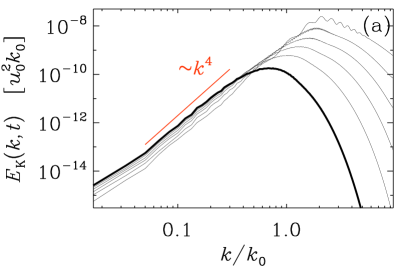
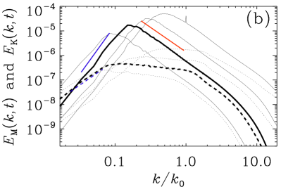

6.2 Helical field decay
The most interesting difference between the decay of MHD turbulence and the purely hydrodynamic case occurs in case the field is helical, due to magnetic helicity conservation. Consider for example the decay of a fully helical magnetic field with energy and helicity in a fixed co-moving volume and integral scale defined by
| (98) |
Assume that there is rough equipartition between the kinetic energy and magnetic energy, and the two fields have the same scale. Then on dimensional grounds, the total energy changes at a rate . Using we get
| (99) |
Noting that is approximately conserved during the decay of the energy, this can be integrated to give
| (100) |
Thus the presence of helicity slows down the decay of the field even further, and more importantly, the coherence scale grows faster than in the nonhelical case. Some earlier numerical simulations seem to show an even slower decay with , (Biskamp and Müller, 1999, 2000)i, while that of Christensson et al. (2001) showed the expected decay of but . However, more recent simulations (Banerjee and Jedamzik, 2004; Kahniashvili et al., 2013; Brandenburg et al., 2015), are consistent with the scaling law given in Eq. (100). Panel c of Fig. 1 gives the results from the DNS by Brandenburg et al. (2015), which shows clearly the inverse cascade of the magnetic field to larger and larger scales.
The effect of having a partial helicity has also been discussed by Banerjee and Jedamzik (2004). It turns out the field decays as if it were nonhelical conserving helicity. As the energy deceases conserving helicity, the field is eventually driven to the fully helical state and subsequently follows the decay law for a helical field. Suppose one starts with the helical fraction at generation, then noting that the initial helicity is conserved while energy decays, fractional helicity subsequently scales as . Then the field will become fully helical at an epoch , and after this decay as if it were fully helical.
6.3 The effect of viscosity
The importance of the viscous force increases secularly with time as the mean free path of the least coupled particle , and hence increases. Recall that the fluid Reynolds number at any scale , is given by
| (101) |
Typically increases faster than as the universe expands; for example for photons . Then the fluid Reynolds number decreases secularly with time. When increases to a value such that , then drops to a value of order unity, and viscous damping damps the modes on the nonlinear scale itself. Both the velocity and magnetic field on this scale are expected to be damped. However, very rapidly increases further so that on all larger scales (or ), and the motions become overdamped. The Lorentz force induces then a fluid velocity got by balancing it against friction, that is , which implies . This small induced velocity does not distort the field significantly, as it leads to a fractional displacement of order . Therefore, the magnetic field inhomogeneities are now frozen in this strong damping regime, a feature is very similar to what obtains for the linear Alfvén waves discussed earlier.
As the comoving mean free path further increases, it becomes larger than the coherence scale of the magnetic field, i.e. . Then one transits from diffusive damping to the free stream damping regime. In this regime the viscous force (in Eq. (43)), is given by , where is the density of the particle species providing the drag, and we have assumed it to be relativistic. This species could be neutrinos just before neutrino decoupling and photons just before recombination. We also define as the density of all the species coupled to the particle providing the drag. As the damping will be large when free stream damping first becomes important, the fluid velocity is given by the balance between the Lorentz force and viscous force, that is
| (102) |
Here is the Alfvén velocity defined using the density of the particle providing the drag. For the modes on the coherence scale, we have intially and thus as in general. The corresponding fluid Reynolds number during the free streaming regime is
| (103) |
This is again much smaller than unity when free stream damping begins as . Thus when free stream damping begins for any mode, the fluid velocity which was already small during the diffusive damping, will remain small. As the universe expands and increases, the free stream damping becomes weaker and the fluid velocity increases. As increases the field will be advected due to flux freezing and in a time all modes which satisfy can oscillate significantly in the presence of free stream damping and as a result be significantly damped. Thus the coherence scale of the field now increases due to the damping and is given by
| (104) |
where we have substituted from Eq. (102). This is exactly the Silk damping scale of the Alfvén wave modes discussed earlier.
Note that the velocity can at most increase to be of order the Alfv’en velocity after which the Lorentz force due to the magnetic field acts to restore the fluid motion. This happens when has grown such that or using Eq. (102), . At this stage the mode which can suffer significant damping satisfies, , and so is actually the mode at the nonlinear scale itself. At the same time, the condition also implies from Eq. (103), that the fluid Reynolds number grows to , with the viscous evolution transiting again to turbulent decay. Thus as pointed out by Banerjee and Jedamzik (2004), the magnetic coherence scale at the end of the viscous period, grows to the value it would have had, as if there had been no viscosity dominated period of evolution at all. The viscous period in this sense just delays the dissipation of the field. It is not of course obvious that or will individually tend to the value they would have had, if the viscous evolution interval was not present, although their product at the end of this phase. However, the simulations of Banerjee and Jedamzik (2004) seem to suggest this is a good approximation.
The above picture holds for example during the epochs when neutrino viscosity is important. A similar evolution also holds during the epoch when photon viscosity is important. However, as the scatterers, electrons and positrons become non-relativistic below , their number decreases rapidly with a corresponding rapid increase of the photon mean free path. Also, after recombination, the photon mean free path increases so rapidly Mpc to the Hubble radius, that free stream damping by photons is abruptly switched off. This leads to a smaller coherence scale and a larger field strength at the end of the photon damping era, compared to the case where the flow would have stayed turbulent all along.
6.4 Summary
The nonlinear evolution of primordial fields can be summarized as follows. During turbulent evolution, the field decays satisfying , , with and , respectively for the , nonhelical cases and for the fully helical case. And when viscosity dominates, the field first freezes during diffusive damping and decays more rapidly during free-stream damping to a value as if the viscous epoch was not present at all. Partially helical fields first decay as if they are nonhelical conserving helicity till the field becomes fully helical; then they decay as for the fully helical case.
These laws are applicable to the scaled comoving magnetic fields, with the conformal time. In the radiation dominated epoch, we have and so , and we can map the above power law scalings directly to that with the expansion factor itself. On the other hand in the matter dominated epoch, one needs a a different set of transformations to map MHD in the expanding universe to flat space (Banerjee and Jedamzik, 2004), where the scaled ’conformal’ time variable satisfies, , with . Thus , and any power law decay of or growth of in scaled time, corresponds to only logarithmic decay/growth in terms of physical time, or scale factor. Thus evolution of the field virtually freezes at the end of the radiation domination epoch, as also found in the detailed numerical calculations of Banerjee and Jedamzik (2004).
These ideas have been put together by several authors to deduce the present day strength and coherence scale of primordial magnetic fields causally generated at the QCD and electroweak phase transitions, after it has gone through epochs of turbulent and viscous decay. An important general feature as discussed above is that in turbulent epochs the field satisfies the condition . Banerjee and Jedamzik (2004) note that this relation is also applicable after reionization, and so derive a general condition for the present day field strength and coherence scale,
| (105) |
A simple estimate for the field itself, can be got assuming the turbulent decay scaling from generation era (, ) to end of radiation era (, eV) and subsequent freezing of the comoving field strength. For nonhelical fields this gives, . Using the conservation of , adopting at the equality epoch, at the generation epoch, and gives
| (106) |
where , is as in Eq. (1) and GeV. For the partial helical case, with initial helical fraction , we have , where is expansion factor corresponding to when the field becomes fully helical. Note that this result is independent of , and putting in numbers,
| (107) | |||||
The corresponding coherence scales can be got from using in Eq. (105).
These simple estimates agree reasonably with the more detailed estimates by Banerjee and Jedamzik (2004). Taking , they give
| (108) |
For as would be relevant to the EWPT and , one gets from Eq. (108), kpc and nG. If fully helical fields could be generated at the QCD phase transition, with generation at , the corresponding values for and are times larger. For a nonhelical fields, assuming and would be smaller, compared to the fully helical case. But predicting how much exactly, will depend on a better understanding of the possible inverse cascade seen for nonhelical fields. Nevertheless, causally generated primordial fields surviving from the early universe phase transitions, could have interesting strengths and coherence scales to influence physical processes in the universe.
7 CMB signals due to Primordial magnetic fields
As the Universe expands it cools sufficiently such that below , the primeval ionized plasma recombines to form neutral atoms. The photon mean free path becomes larger than the current Hubble radius and they can directly free stream to the observer. These photons are seen as the CMB photons today and they dominantly reflect the physical conditions of the universe from the epoch when they last scattered, known as the LSS or last scattering surface. One of the most important ways of detecting or constraining the existence of primordial magnetic fields is via the observations of the CMB temperature and polarization anisotropies (see Subramanian (2006); Durrer (2007) for reviews). The signals that could be searched for include excess temperature (T) anisotropies at both large angular scales and scales below the Silk damping scale, E and B-mode polarization, non-Gaussian statistics and Faraday rotation effects.
CMB anisotropies in general arise in two ways. Firstly, spatial inhomogeneities around the LSS lead to the ‘primary’ anisotropies in the CMB temperature as seen at present epoch. Furthermore, variations in intervening gravitational and scattering effects, which influence the CMB photons as they come to us from the last scattering surface, can lead to additional secondary anisotropies (see Padmanabhan (2002); Dodelson (2003); Subramanian (2005) for pedagogical reviews of CMB anisotropies).
The CMB is described by its brightness (or intensity) distribution. Since the spectrum of the CMB brightness, seen along any direction on the sky , is very close to thermal, it suffices in most cases to give the temperature . The temperature is very nearly uniform with fluctuations at the level of , after removing a dipole contribution. It is convenient to expand the temperature anisotropies at the observer in spherical harmonics (with the dipolar contribution, predominantly produced by the Earth’s motion in the CMB frame, subtracted)
| (109) |
with as is real. In the standard picture, the universe is assumed to have evolved from density fluctuations initially described by a random field, which is almost Gaussian. In this case ’s are also random variables with zero mean and a variance completely described by their power spectrum,
| (110) |
Here we have assumed also the statistical isotropy of field because of which the power spectrum is independent of . Theoretical predictions of CMB anisotropy are then compared with observations by computing the ’s or the correlation function , where if we have statistical isotropy, depends only on . From Eq. (110) and the addition theorem for the spherical harmonics, we have
| (111) | |||||
The mean-square temperature anisotropy, is
| (112) |
with the last approximate equality valid for large , and so is a measure of the power in the temperature anisotropies, per logarithmic interval in space. This particular combination is used because scale-invariant potential perturbations generate anisotropies, which at large scales (small ) have a nearly constant . A convenient characterization of the scale-dependent temperature anisotropy is . One can roughly set up a correspondence between angular scale at the observer , the corresponding value it refers to in the multipole expansion of and also the corresponding co-moving wavenumber of a perturbation which subtends an angle at the observer. One has and where is the comoving angular diameter distance to the LSS and is Gpc, for a standard CDM cosmology. The predicted CMB temperature anisotropy is shown as topmost solid line, top left panel in Fig. 2 (and in Fig. 3 as a dashed-double-dotted line), for a standard CDM model.
Primordial magnetic fields induce a variety of additional signals on the CMB. First, a very large scale (effectively homogeneous) field would select out a special direction, lead to anisotropic expansion around this direction, hence leading to a quadrupole anisotropy in the cosmic microwave background (CMB). (see, for example, Thorne, 1967). The degree of isotropy of the CMB then implies a limit of several nG on the strength of such a field redshifted to the current epoch (Barrow et al., 1997; Adamek et al., 2011).
Primordial magnetogenesis scenarios on the other hand, as we discussed above, generally lead to tangled fields, plausibly Gaussian random, characterized by say a spectrum . The scalar, vector and tensor parts of the perturbed stress tensor associated with such primordial magnetic fields lead to corresponding metric perturbations, including gravitational waves. Further the compressible part of the Lorentz force leads to compressible (scalar) fluid velocity and associated density perturbations, while its vortical part leads to vortical (vector) fluid velocity perturbation. These magnetically induced metric and velocity perturbations lead to both large and small angular scale anisotropies in the CMB temperature and polarization. A helical field can also lead to odd parity, and correlations, not expected for inflationary scalar perturbations.
In addition, the presence of tangled magnetic fields in the intergalactic medium can cause Faraday rotation of the polarized component of the CMB, leading to the generation of new B-type signals from the inflationary E-mode signal. Their damping in the pre-recombination era can lead to spectral distortions of the CMB (Jedamzik et al., 2000), while their damping in the post-recombination era can change the ionization and thermal history of the Universe (Sethi and Subramanian, 2005).
7.1 Scalar modes
The scalar contribution has been the most subtle to calculate, and has only begun to be understood by several groups (Giovannini and Kunze, 2008; Yamazaki et al., 2008; Finelli et al., 2008; Shaw and Lewis, 2010; Bonvin et al., 2013). Three types of contributions to the curvature perturbation are in principle possible. (i) A mode known as the passive mode, which arises before neutrino decoupling, sourced by the magnetic anisotropic stress. (ii) A compensated mode which remains after the growing neutrino anisotropic stress has compensated the magnetic anisotropic stress on large scales (cf. Shaw and Lewis (2010) for detailed discussion). (iii) In addition Bonvin et al. (2013) have stressed the possibility of a constant contribution to the curvature perturbation, which arises when magnetic fields are generated during inflation.
Specifically, the stress tensor (space-space part of the energy-momentum tensor) for magnetic fields in terms of the present day magnetic field value is
| (113) |
In Fourier space, the product of magnetic fields becomes a convolution
| (114) |
| (115) |
where is the Fourier transform of . This can be expressed in terms of the magnetic perturbations to the energy-momentum tensor as
| (116) |
where and are the perturbations in the energy density and anisotropic stress, respectively, as defined in Shaw and Lewis (2010). Also and are respectively the radiation energy density and pressure, and as they are , and are constant. The anisotropic stress can be decomposed to scalar, vector and tensor contributions. The amplitude of the anisotropic stress for scalar perturbations is given by , got by applying the relevant projection operator to (Brown and Crittenden, 2005).
| (117) |
Note that of Shaw and Lewis (2010) is equal to of Brown and Crittenden (2005).
The magnetic stresses are non-linear in the field but we assume that they are always small compared to the total energy density and pressure of the photons, baryons etc. Thus allowing a purely linear treatment of the perturbations. Hence the scalar, vector and tensor perturbations decouple and evolve independently. Prior to neutrino decoupling, the only source of anisotropic stress is the magnetic field. Once the neutrinos decouple, the anisotropic stress due to neutrinos also contributes but with an opposite sign to that of the magnetic field, thus compensating the contribution from the magnetic field on large scales (Lewis, 2004). The post inflationary evolution thus leads to two types of modes (Shaw and Lewis, 2010). The first one, the passive mode, is an adiabatic-like mode but has non-Gaussian statistics. It grows logarithmically in amplitude between the epochs of magnetic field generation and neutrino decoupling, driven by the magnetic anisotropic stress, but then evolves passively after neutrino decoupling. This behaviour has also been confirmed in Bonvin and Caprini (2010) in the context of deriving the magnetic Sachs-Wolfe effect for a causally generated primordial magnetic field. The second, more well-studied perturbation (Giovannini and Kunze, 2008; Yamazaki et al., 2008; Finelli et al., 2008; Paoletti et al., 2009), is called the compensated mode, which is sourced by the residual anisotropic stress and magnetic energy density. And as stated above, a third mode may arise due to the effects of magnetic stresses on the curvature during inflation itself (Bonvin et al., 2013)
The final curvature perturbation as derived using the conformal Newton gauge is given by equation (32) of Bonvin et al. (2013) (see also Shaw and Lewis (2010)),
| (118) |
Here and defined by Bonvin et al. (2013), are proportional to and defined in Shaw and Lewis (2010). Specifically they are normalised by the energy density of the inflaton, rather than radiation. (The power per unit logarithmic interval defined in Bonvin et al. (2013) is also a factor larger than the standard definition used by say Shaw and Lewis (2010) and in CAMB code). The term represents the standard inflationary contribution to the curvature perturbation, while is the result of magnetic stresses during inflation, as estimated by Bonvin et al. (2013). The passive mode contribution is the term, . It incorporates the logarithmic growth in the curvature driven by the uncompensated magnetic anisotropic stress, between the epochs of magnetic field generation and neutrino decoupling . In the radiation-dominated era the conformal time is inversely proportional to the temperature so that . For magnetic field generation epoch such that Gev and Mev, and . The evolution of the curvature perturbation has also been discussed (in synchronous gauge) in Kojima et al. (2010) for the case of an extra source of anisotropic stress canceling the neutrino anisotropic stress. The role of anisotropic stresses on CMB has also been discussed by Giovannini (2010).
It is useful to estimate the relative strengths of the various terms in Eq. (118). We focus on nearly scale invariant spectra, which is perhaps the most interesting case, and also one where the upper limits on the strength of the large scale field from CMB observations is the weakest. In this case, the amplitude of the magnetic inflationary mode is given by , where is the conformal time at the end of inflation. And , is the standard inflationary slow roll parameter, with . It vanishes for purely exponential expansion with constant . The ratio of the magnetic inflationary mode contribution to the passive mode is given by . Note that at Mpc-1, and , and . Thus in general , and the magnetic inflationary mode can dominate the passive mode, if both are induced by the field generated during inflation. The passive mode itself dominates the compensated mode due to the extra factor (Shaw and Lewis, 2010). (In case of fields generated in phase transitions, then the magnetic inflationary mode will not be generated). On the other hand, for a field produced during inflation, in general and thus all magnetically induced scalar perturbations are expected to be subdominant to the standard inflationary mode, if the field is produced during inflation. Much more work on the magnetic inflationary mode is warranted to firm up these conclusions.
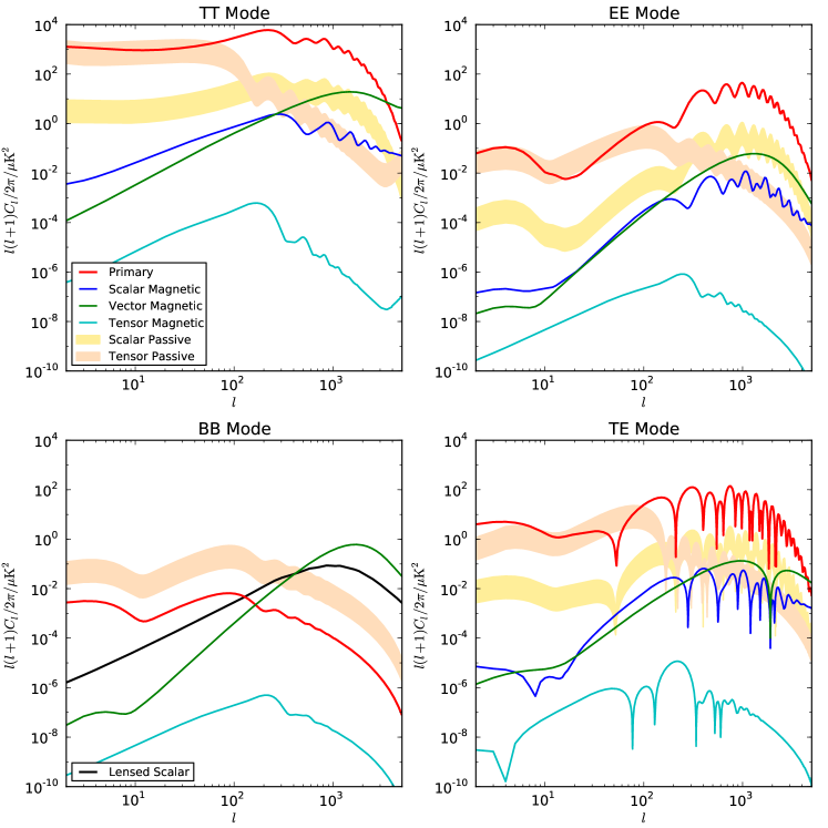
Given the curvature perturbation at late times, and the evolution equation for the baryon-photon fluid, which includes the effect of the Lorentz force, one can calculate the CMB anisotropies due to scalar perturbations. The magnetically induced compressible fluid perturbations, also changes to the acoustic peak structure of the angular anisotropy power spectrum (see, for example, Adams et al., 1996). We show in Fig. 2 the results of such a calculation done using the CAMB code (http://camb.info/ by Lewis and Challinor), modified to incorporate the magnetic effects (Richard Shaw; Private communication). Results are quoted for nG, and spectral indices . In general, for nano Gauss fields, the CMB anisotropies due to the magnetized scalar mode are grossly subdominant to the anisotropies generated by scalar perturbations of the inflaton. They are also subdominant to the anisotropies induced by the magnetically induced tensor modes at large angular scales, and the those induced by vorticity perturbations (vector modes) at small angular scales. They could dominate at intermediate angular scales with , as can be seen in Fig. 2.
7.2 Vector modes
A more important contribution to CMB anisotropies at large , induced by primordial magnetic fields, arises due to the Alfvén mode driven by the rotational component of the Lorentz force (Subramanian and Barrow, 1998b; Mack et al., 2002; Subramanian et al., 2003; Lewis, 2004). Unlike the compressional mode, which gets strongly damped below the Silk scale, due to radiative viscosity (Silk, 1968), we saw that the Alfvén mode behaves like an over damped oscillator, and survives Silk damping down to much smaller scales; (Jedamzik et al., 1998; Subramanian and Barrow, 1998a). The resulting baryon velocity can lead to CMB temperature and polarization anisotropies, peaked below the Silk damping scale (angular wavenumbers ). We estimate these more quantitatively below.
On galactic scales and above, note that the induced velocity due to the Lorentz forces is generally so small that it does not lead to any appreciable distortion of the initial field (Jedamzik et al., 1998; Subramanian and Barrow, 1998a). Hence, the magnetic field simply redshifts away as . The Lorentz force associated with the tangled field , with , pushes the fluid to create rotational velocity perturbations. These can be estimated by using the Navier-Stokes equation for the baryon-photon fluid in the expanding Universe. In Fourier space the rotational component of the fluid velocity satisfies,
| (119) |
Here, as before, is the photon density, the baryon density, and the shear viscosity coefficient associated with the damping due to photons, where is the photon mean free path. The projection tensor, projects , the Fourier component of onto its transverse (rotational) components perpendicular to .
One can solve Eq. (119) in two asymptotic limits. For scales larger than the Silk scale, , the radiative viscous damping can be neglected to get
| (120) |
where , with and the conformal time at recombination. Since , we get for large scales , as estimated earlier. For , a terminal velocity approximation, balancing viscous damping and the Lorentz force gives, , and , where . Thus first increases with and for , then decreases with , with a maximum around the Silk scale.
This leads to CMB anisotropies , due to the doppler effect. For small , we have . Adopting , we have , indicating that significant CMB anisotropies at large can indeed result from the Alfvén mode.
The due to rotational velocity perturbations can be calculated using Hu and White (1996, 1997).
| (121) | |||||
Here is the magnitude of the rotational component of the fluid velocity in Fourier space, and the present value of . There are also contributions from the vector metric perturbation, and the polarization (Hu and White, 1997). But the vector metric perturbation decays with expansion, even including magnetic sources (Mack et al., 2002) and the polarization causes very small corrections to Eq. (121).
The ‘visibility function’ in Eq. (121) determines the probability that a photon reaches us at epoch if it was last scattered at the epoch . We have shown as a solid line in Fig. 7 the visibility function for a standard CDM model. It is peaked about a small range of conformal times, say , around . The spherical Bessel function , projects spatial variations, at the last scattering epoch, to angular (or ) anisotropies at the present epoch. It peaks around , and for a fixed , probe a wavenumber around last scattering.
We can obtain analytic estimates of in two limits. First, for , , and hence vary negligibly for where is significant. So they can be evaluated at and taken out of the integral over in Eq. (121). The remaining integral of over gives unity. Also does not vary rapidly with , for where is dominant (. Thus, can also be evaluated at and pulled out of the integral. The remaining -integral of over can be done analytically, giving
| (122) |
where, is the power per unit logarithmic interval of , residing in the rotational velocity perturbation .
In the other limit, , is slowly-varying in compared to . There is a cancellation due to superposition of oscillating contributions of over the thickness of the LSS. An approximate evaluation of then gives
| (123) |
Note that when , is suppressed by a factor due to the finite thickness of the LSS.
The magnetic power spectrum is normalized using a top hat filter in -space, and taken to be of a power law form; with . We generally adopt h Mpc-1, and is the field smoothed over . is cut-off at , determined by dissipative processes.
We can now put together the above results. Note that the power spectrum of the rotational velocity involves not only , but also a mode coupling integral (see below). For we get (Subramanian and Barrow, 1998b, 2002),
| (124) |
Here, and we have used cosmological parameters for the -dominated model, with , and We also use the fit given by Hu and White (1997b) to calculate , valid for flat universe.
On scales smaller than the Silk scale, where and , but , we get
| (125) | |||||
where . Here is a mode coupling integral
Note that for , is independent of . For a nearly scale-invariant spectrum, say with , and , we get for scales larger than the Silk scale, and for scales smaller than but larger than . Larger signals will be expected for steeper spectra, at the higher end.
One can also do a similar calculation for the expected CMB polarization anisotropy (Seshadri and Subramanian, 2001; Subramanian et al., 2003). Note that polarization of the CMB arises due to Thomson scattering of radiation from free electrons and is sourced by the quadrupole component of the CMB anisotropy. For vector perturbations, what is referred to as the B-type contribution dominates the polarization anisotropy (Hu and White, 1997), unlike for inflationary scalar modes.

We show in Figs. 3 and 4 the temperature and polarization anisotropy for the magnetic field induced vector modes obtained by evaluating the and integrals in Eq. (121) numerically. We retain the analytic approximations to and . These curves show the build up of power in temperature and B-type polarization due to vortical perturbations from tangled magnetic fields which survive Silk damping at high –. The eventual slow decline is due to the damping by photon viscosity, which is only a mild decline as the magnetically sourced vortical mode is over damped. By contrast, in the absence of magnetic tangles there is a sharp cut-off due to Silk damping. Our numerical results are consistent analytic estimates given in Eqs. (124) and (125). They also qualitatively agree with the more detailed calculations presented in Fig. 2 as thin, solid green lines.
A scale-invariant spectrum of tangled fields with Gauss, produces temperature anisotropies at the K level and B-type polarization anisotropies –K between –. Larger signals result for steeper spectra with . Note that the anisotropies in hot or cold spots could be several times larger, because the non-linear dependence of on will imply non-Gaussian statistics for the anisotropies.
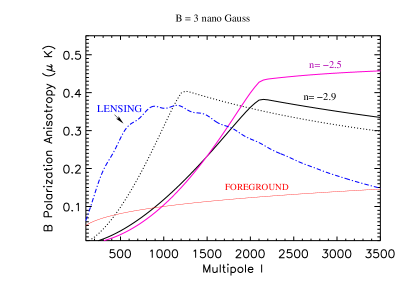
7.3 Tensor modes
The magnetic anisotropic stress due to a stochastic magnetic field also induces tensor or gravitational wave perturbations. These can lead to CMB temperature and polarization anisotropies, but now peaked on large angular scales of a degree or more or small (Durrer et al., 2000; Mack et al., 2002; Caprini and Durrer, 2002). The perturbed FRW metric describing tensor metric perturbation is given by . Here is transverse () and traceless () and obeys the equation
where , a prime denotes derivative with respect to the conformal time, and is the transverse, traceless component of the energy momentum tensor (due to the magnetic field). The gravitational wave affects the photon trajectory and its frequency, and results in change in the CMB temperature. The resulting CMB anisotropy is then computed using
where is a unit vector along the line of sight, and prime denotes a conformal time derivative. The integration is from an epoch , the epoch of last scattering to the present epoch . To make progress one expands and , in a Fourier and polarization basis. The polarization tensor for any Fourier mode is defined as , where form mutually perpendicular unit vectors. We define
The amplitudes then satisfy the damped harmonic oscillator equation,
whose particular solution sourced by the magnetic anisotropic stress is given by (Durrer et al., 2000; Mack et al., 2002),
| (126) |
Here we have modified the argument of the log factor, to take account of the fact that the magnetic anisotropic stress gets compensated on large scales after neutrino decoupling (Lewis, 2004; Shaw and Lewis, 2010). This mode is therefore referred to as the ‘passive’ tensor mode.
We see that the amplitude of a given gravitational wave mode remains constant for small , when it remains outside the Hubble radius. Once it enters the Hubble radius, and , it undergoes damped oscillations, as can be seen from the term in Eq. (126). As smaller scales (larger or ) modes enter the Hubble radius at earlier epoch, they are damped more by the epoch of last scattering. Thus for a nearly scale invariant spectrum of magnetic fields, their tensor mode contribution to CMB anisotropies will be largest at large scales (small ) and will oscillate and decay at smaller and smaller scales. Such a behaviour can indeed be seen in Fig. 2, where the Tensor passive mode signals are seen as top most magenta band at low , in all the panels. The band represents the uncertainty in the value of which is chosen to range from .
Using the formalism described in Durrer et al. (2000); Mack et al. (2002), an analytical estimate of the tensor contribution at small is , for . The tensor mode also contributes to the B-type polarization anisotropy at large angular scales ( or so), with K for . The production of gravitational waves has been used in an indirect manner by Caprini and Durrer (2002) to set strong upper limits on for spectra with or so.
7.4 Faraday rotation due to primordial fields
Another interesting effect of primordial fields is the the Faraday rotation it induces on the polarization of the CMB (Kosowsky and Loeb, 1996; Kosowsky et al., 2005; Campanelli et al., 2004) The rotation angle is
| (127) |
where is the frequency of observation. So this effect is important only at low frequencies, and here it can lead to the generation of B-mode polarization from the Faraday rotation of the inflationary E-mode. From the work of Kosowsky et al. (2005) one can estimate a B-mode signal , for , at . The signals are smaller at smaller . The Faraday rotation signal can be distinguished from the B-mode polarization generated by say vector modes, or gravitational lensing, because of their frequency dependence ().
7.5 CMB non Gaussianity
A crucial difference between the magnetically induced CMB anisotropy signals compared to those induced by inflationary scalar and tensor perturbations, concerns the statistics associated with the signals. Primordial magnetic fields lead to non-Gaussian statistics of the CMB anisotropies even at the lowest order, as magnetic stresses and the temperature anisotropy they induce depend quadratically on the magnetic field. In contrast, CMB non-Gaussianity due to inflationary scalar perturbations arises only as a higher order effect. A computation of the non-Gaussianity of the magnetically induced signal has begun (Seshadri and Subramanian, 2009; Caprini et al., 2009; Cai et al., 2010), based on earlier calculations of non-Gaussianity in the magnetic stress energy (Brown and Crittenden, 2005). Anisotropy and non-Gaussianity can also result during inflationary magnetogenesis in particular models where conformal invariance is broken by coupling to the inflaton (Barnaby et al., 2012; Bartolo et al., 2013; Fujita and Yokoyama, 2013). This new direction of research on CMB non-Gaussianity currently leads to constraints on the field at sub nG level (Trivedi et al., 2014), and promises to lead to tighter constraints or a detection of strong enough primordial magnetic fields (Shiraishi et al., 2010, 2011; Trivedi et al., 2010, 2012, 2014).
7.6 A summary of CMB constraints
We have outlined some of the possible ways one could detect/constrain primordial magnetic fields using the CMB anisotropies and polarization. For a field of nG and a nearly scale-invariant spectrum one predicts CMB temperature anisotropies with a K, at (induced by tensor modes) and (due to the Alfvén mode) and polarization anisotropies about 10 times smaller. Especially interesting is that the vector modes induced by primordial fields can contribute significantly below the Silk scale, where the conventional scalar modes are exponentially damped. Further, the magnetically induced polarization signal will be dominated by B-mode polarization. A unique signature of primordial fields on the CMB is that magnetically induced anisotropies are predicted to be strongly non-Gaussian. Also if fields have helicity, this would induce further parity odd cross correlations, which would not otherwise arise (Caprini et al., 2004; Kahniashvili and Ratra, 2005; Kahniashvili et al., 2014; Ballardini et al., 2015).
The most systematic analysis of CMB constraints has been carried out using the Planck data (Planck Collaboration: XIX et al., 2015). This analysis assumes a spatially flat universe, with the CMB temperature K, a primordial Helium fraction of , three massless neutrinos and lensing effect only for the primary CMB spectrum. It also marginalises over astrophysical residuals and secondary anisotropy contamination, varies a set of 6 standard cosmological parameters, the amplitude of the magnetic field smoothed over scales of 1 Mpc and the magnetic spectral index . Overall this analysis constrains the primordial magnetic field strengths to be less than a few nG. More specifically, using the angular power spectra and the Planck likelihood, the 95 confidence level constraints are nG on Mpc scale with correspondingly, for non-helical fields and nG for helical fields. These tighten to nG for nearly scale invariant fields with , nG for causally generated fields where one expects and nG for any . For the nearly scale invariant case, the limits further tighten to nG if their effects on heating and ionization (Sethi and Subramanian, 2005; Kunze and Komatsu, 2015; Chluba, Paoletti, Finelli and Rubino-Martin, 2015) (see Section 8) are included. The limits from the magnetically induced tensor and compensated scalar bispectrum are at the 3 nG level. It has been pointed out by Trivedi et al. (2012, 2014) that stronger sub nG limits are possible from analysis of the CMB trispectrum. Moreover stronger limits would also be potentially possible from the magnetic inflationary mode (Bonvin et al., 2013). A comparison of the estimated trispectrum from the scalar passive mode and Planck 2013 limits on CMB non-Gaussianity, gave nG, and that from the magnetic inflationary mode suggests nG (Trivedi et al., 2014).
Primordial magnetic fields have also been constrained by the POLARization of the Background Radiation (POLARBEAR) experiment from the detection of the B-mode polarization at high (Polarbear Collaboration: et al., 2015). Comparing the theoretically expected B-mode polarization signal from vector mode gives a limit nG at the 95% confidence level. There has also been a claimed detection of the B-mode polarization on degree scales (low ) by the BICEP2 experiment (BICEP2 Collaboration: et al., 2014), which could be due to tensor modes from the inflationary era, or potentially also seeded by primordial magnetic fields. This signal is however now thought to due to contamination by dust emission (Keck Array and BICEP2 Collaborations et al., 2016; BICEP2/Keck and Planck Collaborations: et al., 2015). Even were it present, the amplitude of the observed B-mode polarization is difficult to explain as due to primordial magnetic fields (Bonvin et al., 2014), given the constraints from the CMB trispectrum (Trivedi et al., 2014). However the B mode induced by such fields, combined with the dust contribution, could ease the required level of tensor modes from standard inflationary models (Bonvin et al., 2014). Clearly, the detection of B-modes at both large and small angular scales, and also the limits (or detection) of non-Gaussianity in both temperature and polarization anisotropies, are likely to provide the strongest future CMB probes of primordial magnetic fields.
The current limits on primordial magnetic fields from CMB observations are summarized in Table (1), where we have also given constraints coming from other physical probes discussed below.
| Probe | Magnetic modes | Upper limit (nG) | Reference |
| CMB Power Spectra | scalar, vector & tensor | 4.4 (non helical, general) | Planck-2015 |
| scalar, vector & tensor | 5.6 (Helical, general) | Planck-2015 | |
| scalar, vector & tensor | 2.1 (Scale invariant) | Planck-2015 | |
| Ionization History | 0.7 | Planck-2015 | |
| CMB Polarization | Vector, B Mode | 3.9 | POLARBEAR |
| CMB Bispectrum | energy density | 22 | Seshadri and Subramanian (2009) |
| (Compensated scalar) | |||
| Passive-scalar | 2.4 | Trivedi et al. (2010) | |
| Compensated-scalar | 3 | Planck-2015 | |
| vector | 10 | Shiraishi et al. (2010) | |
| Passive-tensor | 3.2 | Shiraishi and Sekiguchi (2014) | |
| Passive-tensor | 2.8 | Planck-2015 | |
| CMB Trispectrum | energy density | 19 | Trivedi et al. (2014) |
| (Compensated scalar) | |||
| Passive-scalar | 0.6 | Trivedi et al. (2014) | |
| magnetic inflationary mode | 0.05 | Trivedi et al. (2014) | |
| (Bonvin et al., 2013) | |||
| Reionization | 0.059-0.358 | Pandey et al. (2015) | |
| Weak Lensing | Pandey and Sethi (2012) | ||
| Lyman- forest | Pandey and Sethi (2013) | ||
| Faraday Rotation | uniform to 50 Mpc | 1-6 | Blasi et al. (1999) |
| uniform to 1 Mpc | 0.5-1.2 (2 ) | Pshirkov et al. (2015) | |
| Absence of GeV halo from Tev Blazars | G | Neronov and Vovk (2010) | |
| (Lower Limit) | () | Tavecchio et al. (2011) | |
8 Primordial magnetic fields post recombination
After recombination, the ionized fraction decreases by several orders of magnitude by , finally reaching a value of for (for details see Peebles (1993)). However, the residual free electrons are still sufficient in density to carry the currents required to sustain primordial magnetic fields. In the standard picture, the matter temperature continues to follow the CMB temperature, both falling as for . At smaller redshifts, matter ’thermally’ decouples from the radiation and the matter temperature falls as . This thermal and ionization history holds up to , when the formation of first structure can lead to reionization and reheating. Primordial magnetic fields can alter this picture in several interesting ways (Sethi and Subramanian, 2005).
First, the magnetic fields exert forces on the electron-ion fluid, but not on the neutral atoms, causing a relative drift velocity and hence a friction between these components. This can lead to the dissipation of the magnetic energy, called ambipolar diffusion, into the intergalactic medium. Also the increased photon mean free path due to recombination, leads to a reduced viscosity and increased fluid Reynolds number, leading to the possibility of generating decaying fluid turbulence. These processes will affect the thermal and ionization history of the universe. In addition the Lorentz force due to tangled primordial magnetic fields, can also induce density perturbations, which grow due to gravitational instability and cause early formation of structures in the universe. Such enhanced density perturbations can also lead to weak lensing signatures, and together with the altered ionization history lead to new signals in the 21 cm and the CMB. We consider some of these effects in more detail below.
8.1 Magnetic field dissipation post recombination
A rough estimate of the field strength which will result in significant changes to the ionization and thermal history of the universe can be obtained as follows. If, at a certain epoch, a fraction of magnetic field energy is dissipated into the IGM then it will typically raise it to a temperature: ; with and . Taking , this give for . For , this could be an overestimate because, owing to inverse Compton scattering off CMB photons, matter temperature cannot increase much above CMB temperature. The fraction of the energy dissipated will depend on the magnetic field power spectrum and also on the rate of energy dissipation compared to the expansion rate. However it does give a rough estimate of the magnitude of that are of interest.
The volume rate of energy dissipation due to ambipolar diffusion is (Cowling (1956) Eq. (27)).
| (128) |
Here , , and are the densities of neutral particles mostly hydrogen, ionized hydrogen, and total baryon density, respectively. Also (Shu, 1992); where is the ion-neutral relative velocity and is the cross section for the collision between ions and neutrals. For , independent of the relative velocity of ions and neutrals (Shu, 1992). This energy is deposited into the neutral component of the medium. However collisions between electrons, protons, and neutrals lead to rapid thermalization (Madau et al., 1997). The volume rate of energy deposition in electrons, is , where is the ionization fraction. It can be seen from Eq. (128) that the rate of dissipation is dominated by the smallest scale (largest ) for the scale-free magnetic field power spectrum. This will correspond to the large-k cut-off, in Eq. (90).
Figure 5 and 6 show the ionization and thermal history of the universe for some interesting values of for both delta function and power law power spectra, as computed by Sethi and Subramanian (2005). For delta function power spectrum, the power is assumed to be at and for the power law power spectrum is defined as RMS value smoothed at . We see that the IGM can indeed be significantly heated and ionized for nG. Similar results have also been obtained in subsequent calculations of heating and ionization by primordial magnetic fields (Schleicher et al., 2008; Schleicher, Banerjee and Klessen, 2009; Kunze and Komatsu, 2015; Chluba, Paoletti, Finelli and Rubiño-Martín, 2015).
There are several consequences of such heating and ionization: (i) The thermal Jeans mass is raised by the increase in the IGM temperature which affects subsequent structure formation. (ii) The number density of free electrons which can catalyze formation of molecular hydrogen is increased. This results in a larger molecule abundance at the onset of in the first galaxies (Sethi et al., 2008; Schleicher, Galli, Glover, Banerjee, Palla, Schneider and Klessen, 2009), and its subsequent influence on the formation of first stars. (iii) The extra ionization also modifies the visibility function for the CMB photons. Recall that the visibility functions measures the normalized probability that a photon last scattered between and , or a redshift interval . We show in Fig. 7 visibility functions for the some representative models in comparison with the standard visibility function. One can see that the effect of ambipolar diffusion, with nG, can cause significant changes to the visibility function, and this will also lead to distortions in the CMB anisotropies. Such changes are only beginning to be explored (Chluba, Paoletti, Finelli and Rubiño-Martín, 2015), and appear to provide strong nG level constraints on the primordial fields (Planck Collaboration: XIX et al., 2015).


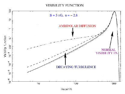
8.2 Primordial magnetic fields and structure formation
In the radiation dominated era, we saw that the pressure associated with a primordial magnetic field is generically much smaller than the pressure of the baryon-photon fluid. Therefore any non-uniform magnetic field would only generate motions which are nearly incompressible. However, as we mentioned earlier, once any particular scale becomes smaller than the photon mean free path, the baryons and photons begin to decouple for perturbations on this scale. Then this ‘mode’ enters the free-streaming regime, where the radiative damping transits from being diffusive to free-stream damping. More importantly, the baryons no longer feel the pressure of the photons, and there is a dramatic fall in the fluid pressure, by a factor of order the very small baryon to photon ratio . Of course this happens for all scales after the recombination era, when atoms form, and the electron density drops so drastically that the photon mean free path becomes of order the Hubble radius. As a result, the pressure of the non-uniform magnetic field, associated with what might well have been an Alfvén-type mode, can no longer be ignored. This will now also induce gravitationally unstable, compressible motions. The resulting growth in density perturbations in the baryons lead, via their gravitational influence, to density perturbations in any dark matter component. Such perturbations then grow due to their self gravity and when they become comparable to the background density, they become non linear, and cause the collapse of these regions, forming structures. We study this magnetically induced structure formation in this section.
Let us assume that the perturbations in density and velocity are small enough so that non-linear terms in the perturbed density and velocity can be neglected. In the Euler equation (Eq. (83)), we neglect the non-linear term, and take the density of the baryonic component to be , where is the unperturbed FRW background density of baryons, and , its fractional perturbation. This equation has to be supplemented by the continuity equation for , the induction equation (30), with , and the Poisson equation for the gravitational potential, . We have (Wasserman, 1978; Kim et al., 1996; Subramanian and Barrow, 1998a; Sethi and Subramanian, 2005),
| (129) | |||||
| (130) |
| (131) |
| (132) |
We recall that all spatial derivatives are with respect to co-moving spatial co-ordinates. In the Poisson equation, we have taken account of the possibility that there may be other forms of matter, like collisionless dark matter (DM) whose background density is given by and its fractional density perturbation by . Thus is the sum of the perturbed density due to both the baryonic plus dark matter. We shall adopt the equation of state , where is the sound speed and the mean molecular weight (for fully ionized hydrogen , with the proton mass).
In treating the resulting evolution, it is usual to assume firstly ideal MHD (), and further that the perturbed velocity does not significantly distort the initial magnetic field (Wasserman, 1978; Peebles, 1980)). So one takes , which solves the induction equation (131), if and are neglected. Then the perturbations to the Lorentz force, due to the perturbed magnetic field, is subdominant with respect to the zeroth-order contribution of the Lorentz force itself. Of course, this approximation will break down once significant peculiar velocities have been developed, as will always happen on sufficiently small scales, or at sufficiently late times, for any given magnetic field strength. For galactic scales, it turns out that the distortions to the magnetic field will become important only at late times, even for . Taking the divergence of Eq. (129), substituting for from Eq. (130), using Eq. (132) and the equation of state, leads to the evolution equation for (see Wasserman (1978) for the case without dark matter),
| (133) | |||||
where the source term is given by
| (134) |
Here, is the baryon density at the present time, . We see from Eq. (133) that perturbations in the baryonic fluid are generated by any inhomogeneous magnetic field even if they were initially zero. These perturbations can grow due to gravity (the first two terms on the right hand side of Eq. (133)), are damped by the expansion of the universe and radiative viscosity (respectively the 2nd and 3rd terms on the LHS of Eq. (133)). Further baryonic pressure can provide support against collapse on small scales (the 4th term on the LHS of Eq. (133)).
If we assume dark matter to be cold, one can also derive a similar equation for its fractional perturbed density (Peebles, 1980; Padmanabhan, 2002),
| (135) |
The dark matter perturbations are not directly affected by the magnetic field, but are coupled to the field via the baryonic perturbations by gravity.
After recombination, the mean-free-path of the photon increases rapidly to a value exceeding the Hubble radius, viscous damping becomes subdominant compared to expansion damping, and can be neglected. Also, for large enough scales, larger than the thermal Jeans mass we can neglect the fluid pressure term. The perturbation equations can then be solved by first defining, with . Then Eq. (133) and (135) become
| (136) |
The homogeneous solutions correspond to perturbations generated by sources before recombination, e.g.during inflationary epoch. We focus here on the particular solution, whereby density perturbations are induced by inhomogeneous magnetic field. Then the solution to Eq. (136) for , in a spatially flat universe is
| (137) | |||||
The initial time corresponds to the epoch of recombination as the perturbations cannot grow before this epoch. In the second line in Eq. (137), we have used the Einstein equation valid at early times to estimate and also retained only the growing mode solution. Using this solution, one can show that the fastest growing mode also has and so both the baryonic and the dark matter perturbations grow at the same rate.
We can make an estimate of the typical scales which can grow for nano Gauss field strength by using Eq. (137). We adopt , , and approximate . Here is the Alfvén velocity relevant in the post-recombination epochs using the baryon density, and is given by
| (138) | |||||
where is the magnetic field smoothed on a scale at time . We get
| (139) |
We see that galactic scales can become non-linear with by the present, if all the field is concentrated on this scale. Subgalactic scales can become non-linear even earlier for nano-Gauss strength fields. We give a more precise calculation of this effect below.
The power spectrum of matter perturbations can written as,
| (140) |
and can be computed given the magnetic power spectrum (Gopal and Sethi, 2003). In particular, for a nearly scale invariant magnetic spectrum, we find that (since involves two spatial derivatives). This steep increase in will lead to the magnetically induced density perturbations to dominate those induced by inflation at small enough scales for , as can be seen in Fig. 8 from Pandey et al. (2015). This feature also provides the potential to constrain the strength of the primordial field on subgalactic scales by using observations of weak gravitational lensing (Pandey and Sethi, 2012) and the Lyman- forest clouds (Pandey and Sethi, 2013).
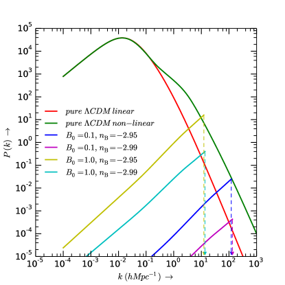
Note that the field gets distorted by the induced motion for all scales smaller than a nonlinear scale say where, . This scale is also approximately equal to the magnetic Jeans length, below which the distortion of the field can lead to magnetic pressure gradients which counteract the gravitational collapse (Kim et al., 1996; Subramanian and Barrow, 1998a). In a linear analysis the proper magnetic Jeans’ wave number, say , can be got from equating the two terms: , giving
| (141) |
The first term incorporates gravitational instability, while the second one the restoring effects due to magnetic pressure. Noting that , the above condition is equivalent to the condition
which is explicitly very similar to the condition determining the nonlinear scale. Interestingly, the comoving Jeans scale , and the comoving Jeans’ length , do not depend on time, at early epochs where the universe is matter dominated; and assuming that the field even at the scale just redshifts as , without significant distortion (Subramanian and Barrow, 1998a). This is because in this case and and hence is constant with time. So any scale which is linear/nonlinear just after recombination, is approximately linear/nonlinear at all epochs (until the vacuum energy starts dominating). Putting in numerical values we get
| (142) |
where is the redshifted value of the field smoothed on the scale . Perturbation growth is suppressed below the magnetic Jeans scale. This is shown schematically as a sharp cut-off in the power spectrum in Fig. 8. The first structures to collapse will have scales close to the magnetic Jeans’ scale .
A standard measure of the stochastic density perturbation is the mass dispersion smoothed over a given radius . In the real space representation one first defines a smoothed out density perturbation field as a convolution of with a window function of radius . Then looks at the dispersion of this quantity. This can then be calculated more conveniently in Fourier space
| (143) |
Here is the window function; for example one can use a Gaussian window function with . The usefulness of lies in the fact that its value roughly determines when a structures on a given scale can collapse. For spherically symmetric perturbations, collapse of a structure corresponds to (Peebles, 1980). Of course for a power spectrum with a cut-off the first collapses will be more pancake like. And there is the added complication of taking account of magnetic pressure effects. Nevertheless it seems reasonable to demand that for the formation of structures. For , the matter power spectrum is , where now is the rms value filtered at scale (Gopal and Sethi, 2003). This gives . For , , and so from Eq. (142) does not depend on the value of . Therefore the redshift at which the first structures collapse becomes nearly independent of the value of , although the mass contained in these structures, which depends on the scale , does depend on , through the dependence. For , , and therefore, even though first structures might form early, the formation of larger structures is suppressed.
In Figure 9 we show the evolution of for the power law magnetic spectra with , for . We can adapt the standard Press and Schechter (1974) type prescription to compute the abundance of objects (Peebles, 1980; Padmanabhan and Subramanian, 1992; Padmanabhan, 2002). For the power law models with nearly scale invariant spectrum, with say , we see from Figure 9, that the first structures can collapse at high redshift . This can significantly influence the reionization of the universe. Also, as beyond the Jeans scale collapse of larger structures occur much later. This means that even though magnetic fields can induce the formation of first structures, it would have less impact on the formation of galactic and larger scale structures at the present epoch. For the total mass of a collapsed halo , which is much smaller than a typical galaxy. For a field , the mass of the first collapsed objects will be smaller, by a factor . Therefore the first structures to collapse would be sub-galactic.
From our discussion above we can conclude that (i) collapse of first structures could have commenced for , (ii) only a small fraction of mass range close to the magnetic Jeans’ scale collapse (iii) the collapse redshift is nearly independent of the strength of the magnetic field, if the magnetic field is specified as rms filtered at the Jeans scale and (iv) the mass of the first collapsed objects will be sub-galactic their exact value depending on . These conclusions hold for magnetic field strengths for which the magnetic Jeans’ length exceeds the thermal Jeans’ length.

8.2.1 Reionization signals
The early formation of subgalactic structures in the presence of primordial magnetic fields, can significantly add to the ionizing photon budget and lead to an early onset of reionization (Sethi and Subramanian, 2005; Tashiro and Sugiyama, 2006a). Note that the universe, which was predominantly neutral after recombination, transited to an ionized state after the first stars formed and emitted ionizing radiation. This period is known as the epoch of reionization (EOR), and its understanding is one of the outstanding challenges of modern cosmology. Observations of the spectra of high redshift quasars have revealed the existence of neutral hydrogen (HI) at redshifts (Fan et al., 2006). Meanwhile the detection of temperature-polarization cross-correlation and the polarization-polarization correlation at large angular scales () in the WMAP and Planck data have given firm evidence that the universe reionized by (Hinshaw et al., 2013; Planck Collaboration: XIII et al., 2015). The presence of primordial magnetic fields could well strongly impact on EOR predictions, and one can in turn constrain such fields from observations related to the EOR.
In Fig. 10 we show the reionization history for two values of magnetic field strength and a standard CDM model with zero magnetic fields. The magnetic spectrum is fixed to be nearly scale invariant with a spectral index . The reionization of the universe is modeled as described in Sethi (2005); Sethi and Subramanian (2009). In this model, an HII sphere is carved around collapsed haloes. Reionization proceeds as more sources are born and as the radius of the HII region around each source increases. It is completed when the HII regions coalesce. The formation rate of dark matter halos is computed as the time derivative of halo abundance which in turn is derived using the Press-Schechter formalism (Press and Schechter, 1974). The radius of the HII region is computed by following its evolution around a source with a given photon luminosity (in ) which is assumed to grow linearly with the halo mass; we fixed the fiducial value of the photon luminosity to be at the mass scale (see e.g. (Sethi, 2005)). The baryons in the IGM are assumed to be clumped with a clumping factor of . The figure shows the evolution of the ionized fraction of the IGM, , adopting for nG and nG respectively, and , for the CDM model. All the reionization histories are normalized to obtain an optical depth of to scattering off the ionized electrons between .
This photon luminosity can be cast in terms of the star formation efficiency, and escape fraction of hydrogen-ionizing photons from star-forming halo. The adopted value for the zero field standard model is such that both the star formation efficiency and escape fraction are roughly , assuming a Scalo IMF for the forming stars. We see from Fig. 10 that one needs a much lower efficiency of star formation (about 25 times lower for nG) for models with primordial magnetic fields, to achieve the same degree of ionization as a standard CDM model (Sethi and Subramanian, 2009). Note that due to the uncertainties associated with both star formation and galaxy formation in presence of strong fields, it is not easy to derive very precise constraints on primordial fields. For some recent efforts in this direction see Pandey et al. (2015), who infer sub nG limits on for nearly scale invariant spectra.

8.2.2 Redshifted 21 cm signatures
The most direct approach to study the EOR is through observations of the redshifted 21-cm line of the neutral hydrogen (Furlanetto, 2016). There is substantial on-going effort in that direction and this also remains one of the primary goals of upcoming and future radio interferometers like the SKA 333www.skatelescope.org/pages/page_sciencegen.htm (Koopmans et al., 2015; Pritchard et al., 2015), and its percursors (e.g. LOFAR 444www.lofar.org). Since primordial magnetic fields cause changes in the matter power spectrum and also in the thermal and ionization history of the universe, they would leave characteristic imprints on the redshifted 21 cm emission. These signals have been worked out by several authors (Tashiro and Sugiyama, 2006b; Schleicher, Banerjee and Klessen, 2009; Sethi and Subramanian, 2009).
There are two types of signals which are usually considered; the global HI signal and the fluctuating component. The global HI signal is observable at the redshifted HI hyperfine transition frequency (), against the CMB, the only radio source at high redshifts. As the matter temperature falls off faster with expansion than the CMB temperature below a , the global HI signal is generally expected to be seen in absorption against the CMB. However in the presence of sufficiently strong primordial fields, there are two effects which can alter this expectation. First the dissipation of tangled magnetic fields can significantly alter the thermal history of the universe (Sethi and Subramanian, 2005). Moreover, the build-up of the Lyman- radiation during the reionization era, which determines the spin temperature of the HI line, depends on the mass function of collapsed haloes. As we noted above primordial fields can enhance the abundance of such small mass halos, and also lead to changes in the .
The global HI signal in the post-recombination era predicted by the calculations of Sethi and Subramanian (2009) is shown in Fig. 11, for some magnetic field models and for a standard CDM model with zero field (Sethi, 2005). The figure shows that unlike the usual case with zero magnetic fields, the HI signal in the magnetised universe is only observable in emission throughout the post-recombination era. This is mainly because the matter temperature does not fall below the CMB temperature for the magnetic field models considered (see also Schleicher, Banerjee and Klessen (2009)). The lack of detection of the HI in absorption could therefore be one signal for the presence of primordial magnetic fields.

The fluctuating component of the HI signals also gets altered in the presence of primordial fields (Sethi and Subramanian, 2009). Note that this component is determined by density inhomogeneities in HI resulting both from density fluctuations in matter and also the result of inhomogeneous ionization. We saw that the matter spectrum induced by nearly scale invariant primordial fields has a sharp rise which is then sharply cut-off at the magnetic Jeans scale (cf. Fig. 8). Such a sharp feature leads to corresponding oscillations in the HI angular correlation function, with a scale length which increases with increasing value of the magnetic field strength. Detecting such oscillations could point to the influence of primordial magnetic fields and also help in determining the field strength. Another major difference between the CDM model and the magnetic field scenario, is in the scale of the signal. Both the density coherence scale and the scale of ionization inhomogeneities turn out to be typically larger in the CDM case (Sethi and Subramanian, 2009).
8.2.3 Weak lensing signatures
Another possibility to directly probe the excess power in the matter power spectrum induced by primordial fields is via weak gravitational lensing (Bartelmann and Schneider, 2001; Munshi et al., 2008). In such lensing the light rays of distant galaxies are deflected by the intervening inhomogeneities resulting in the shearing of their shapes. Galaxies are also intrinsically elliptical. Thus the shearing distortion caused by weak lensing has to be measured statistically by looking at the shapes of a large sample of background galaxies, and calculating the shear correlation function.
The shear field due to scalar density perturbations is to leading order curl-free and is referred to as an E-type field. Thus typically one decomposes the observed shear signal into an E (non-rotational) and B (rotational) components. The level of B-modes can also used to estimate systematic errors in the data. The shear correlations due to the matter power spectrum induced by primordial fields has been calculated by Pandey and Sethi (2012). They find that, for nearly scale invariant spectra and nG field strengths on Mpc-1 scales, primordial fields lead to an excess in the shear correlation function on few arc min angular scales, compared to a standard CDM model. A comparison to the observed data from Fu et al. (2008) was used by Pandey and Sethi (2012) to set upper limits on primordial fields at the nG level.
8.2.4 Influence on Lyman- clouds
The matter power spectrum at small spatial scales can also be sensitively probed from observations of the Lyman- forest absorption lines in the spectra of high redshift quasars (Croft et al., 2002; McDonald et al., 2005). These lines are thought to trace the mildly over dense IGM and so reflect the matter power spectrum. There are of course uncertainties related to the mapping between dark matter and baryons, and the background radiation which keeps the IGM ionized. Typically numerical simulations including the effect of baryonic physics are needed to infer the Lyman- flux power spectrum (Viel et al., 2004), but one can also use semi-analytic models (Bi and Davidsen, 1997; Choudhury et al., 2001).
Pandey and Sethi (2013) have use semi-analytical methods to simulate density fluctuations along the line of sight, including the contribution of matter perturbations due to primordial magnetic fields. They compare the effective Lyman- opacity with the data given by Faucher-Giguère et al. (2008), and derive an upper bound on the magnetic field strength of about nG for a range of nearly scale invariant magnetic field power spectrum
8.3 Constraints from Faraday rotation observations
The polarization plane of a linearly polarized EM wave with wavelength , when propagating through a magnetized plasma, with electron density and line of sight magnetic field , gets rotated by an angle
| (144) |
Here is the initial polarization angle within the source, the electron charge, electron mass, and the integral is over the line of sight to the source which is at a distance . We can separate out the dependence and write , where is called the Faraday rotation measure. Its determination for a distant polarized source, like a high redshift radio source, probes the magnetic field, including any primordial component, along the line of sight to the source.
In the cosmological context, the observed wavelength will be related to that in the medium at redshift , by Then , where now
| (145) |
with now . From Einstein equation, and and so this gives
| (146) |
where and are present day matter and dark energy densities in unit of the critical density. For an estimate of the resulting , assume an uniform field which dilutes with as , and that the IGM is ionized with . Then one can integrate Eq. (145) exactly to get
| (147) | |||||
where the numerical value is got by normalizing to a redshift . We have also normalised by its expected value for a fully ionized universe with . On the other hand, if the field is random, with an integral scale , then the mean value of would be zero but its rms value, would be smaller than that given in Eq. (147) by a factor of order . Thus, assuming a homogeneous universe, an upper limit to the IGM contribution to rad m-2 by , results in upper limit of a nG for the homogeneous field, and an upper limit nG for a field coherent on a Mpc scale.
It was however pointed out by Blasi et al. (1999) that the universe for redshifts of interest is far from homogeneous, as indicated by the Lyman- forest absorption lines, thought to arise in mildly over dense regions of the IGM. The resulting RM would then be larger in such an inhomogeneous universe, both because the density in such regions would be larger and the magnetic field would be larger if it is flux frozen. Assuming and a log normal density distribution for (Bi and Davidsen, 1997), these authors simulated the RM resulting from a large number of random lines of sight to high redshift quasars, until . Including the IGM inhomogeneity implied by the Lyman- forest, results in more than an order of magnitude increase in the predicted RM, a large scatter and also a much less sensitivity to the coherence scale. Comparing with the then existing data of Welter et al. (1984), Blasi et al. (1999) set upper limits of a nG for horizon scale fields, 6 nG for fields coherent on scales of 50 Mpc. Using the RM data from the NVSS survey, Pshirkov et al. (2015) set stronger constraints of nG on horizon scale fields and nG at the 2 level on fields with Mpc coherence lengths. These limits are especially valuable as they use a completely independent technique. They are also likely to improve considerably with the advent of new generation of radio telescopes like the SKA (Taylor et al., 2015; Johnston-Hollitt et al., 2015). There have been interesting work on RM due to magnetic fields in the IGM using cosmological simulations (Akahori and Ryu, 2011; Ryu et al., 2012) and techniques for their detection Akahori et al. (2014), and it would be of interest to extend such studies to include a primordial component.
8.4 Constraints from Gamma ray observations
Recent developments in gamma ray astronomy has provided an intriguing possibility to detect and constrain very weak magnetic fields in the IGM. The basic idea reviewed in detail by Durrer and Neronov (2013) is the following: Suppose we have a source of very high energy gamma rays in the Tev range, like a blazar. These TeV photons can interact with the low energy (eV) photons in the IGM, the extragalactic background light (EBL), and produce a beam of electron-positron pairs. The resulting pairs are highly relativistic and in turn inverse scatter of the much more abundant CMB photons leading to GeV gamma rays. These Gev gamma rays should be detectable by telescopes like Fermi (Atwood et al., 2009), as a gamma ray source associated with the Tev source. However in several blazars where the TeV emission is detected, the corresponding secondary GeV cascade emission is not.
Neronov and Vovk (2010) suggested that this could be explained by the presence of weak intergalactic magnetic fields. In the presence of such fields, pairs get deflected by the magnetic field. As one sees the GeV gamma ray only when the highly relativistic electrons and positrons move towards the observer, this means that we see the GeV photons from a direction displaced from the direction of the primary emission. Thus in the presence of a magnetic field, the secondary GeV source becomes more extended, and its surface brightness could drop below the detectability threshold of Fermi. This was then used to put a lower limit on the IGM field.
We now give more quantitative estimates following Neronov and Vovk (2010); Durrer and Neronov (2013). First, the necessary condition for a TeV photon with energy to interact with an EBL photon of energy and create electron-positron pairs is that the geometric mean of the two photon energies has to be larger than the electron rest mass. That is , which implies one needs a primary photon energy GeV. The mean free path for gamma rays above this threshold energy is (Neronov and Vovk, 2010), Mpc, where accounts for uncertainties in the EBL intensity. Thus the Tev photons propagate far away from their source, in general into the void regions of the IGM, before pair creation take place, and the gamma ray constraints therefore probe the magnetic field in the general IGM.
The created pairs have an energy and so a relativistic gamma factor . The inverse Compton scattering of the CMB photons off these electron then produce secondary gamma rays with energy GeV, where we have used the fact that typical energy of the CMB photon eV. The mean free path for such inverse Compton scattering is Mpc, much smaller than the mean free path for pair creation. Thus inverse compton scattering of the CMB drains the energy from the pairs, a short distance after they are created.
Now the Larmour radius of a relativistic electron is given by Mpc. Thus while the electron traverses a distance before it loses energy to inverse compton scattering, it will be deflected by an angle
| (148) |
assuming the field is coherent on scales much larger than . If the coherence scale of the field is much smaller than than , then the deflection of the charged particle performs a random walk in angle. Then the deflection angle only grows as of the number of steps , and . This gives
| (149) |
The size of the extended GeV cascade source , can be estimated from the Geometry of the problem, where the blazar (B), the observer (O) and the source of cascade gamma rays (S) form a triangle, with angle and . We have , where is the angular diameter distance to the blazar. Thus , where is the optical depth for TeV gamma rays from a source at distance , due to absorption by the EBL. Note that and the source size is larger for lower energy particles and in higher magnetic fields. If this deflection becomes greater than the PSF of the telescope, then the surface brightness of the secondary gamma ray source will decrease.
From the non detection of the secondary gamma ray emission by Fermi telescope, Neronov and Vovk (2010); Tavecchio et al. (2011) deduce a lower limit on the magnetic field in the IGM of G, provided . In the opposite limit the limit becomes more stringent and the lower limit increases as with decreasing . These limits are derived assuming that the cascade emission by the source becoming suppressed due to source extension. Another possibility is that there is large time delay between the direct primary emission and the secondary cascade emission. Such a time delay is expected because for seeing the secondary emission, the TeV gamma rays have to first propagate from B to S and then the secondary gamma rays propagate from S to O, where as the primary emission is seen directly along the path B-O. This lowers the limits on the magnetic field by an order of magnitude or so (Dermer et al., 2011; Taylor et al., 2011).
The basic idea that the relativistic beam of plasma loses its energy primarily to inverse Compton emission against the CMB, has been questioned by Broderick et al. (2012), who argue that plasma instabilities can drain the energy from the beam at a faster rate. Whether this indeed obtains also depends on the efficiency of the nonlinear Landau damping, which can suppress the growth of the instability and stabilize the beam. There is however disagreement about the range of parameters for which nonlinear Landau damping is important; while Miniati and Elyiv (2013) favor the plasma instabilities being stabilized, Schlickeiser et al. (2012); Chang et al. (2014) do find that plasma instability to be important. As pointed out by Durrer and Neronov (2013), the development of plasma instabilities is highly sensitive to the angular and energy distribution of the particles in the beam. A recent particle-in cell simulations also shows that, while plasma instabilities broaden the beam distribution, they do not provide enough energy loss to account for the missing GeV photons, and so magnetic field deflections would then still be important (Kempf et al., 2016). Thus much more work is perhaps needed to settle this issue.
Of relevance in this context is some intriguing work by Tashiro et al. (2014); Chen et al. (2015), who examine a parity-odd triple correlator of -ray arrival directions in Fermi-LAT data, from possibly unseen blazars. They find a non-zero for certain energy bins, which seems to indicate the existence of a helical (left-handed) IGM field G on 10 Mpc scales. As these -rays are actually detected, the issue of whether plasma instabilities drained some energy from the beam becomes irrelevant. Of course a positive detection of an extended halo of GeV emission around TeV blazars or a time delay effect, would provide more conclusive evidence for the intergalactic magnetic field. Nevertheless, -ray observations at present appears to be the only manner in which such weak fields can be potentially detected, and is therefore very exciting!
9 Astrophysical batteries and dynamos
Primordial magnetic fields are the main focus of this review. However, it is also interesting to mention astrophysical batteries which can generate coherent seed magnetic fields in the late universe. In addition magnetic fields are currently only detected in systems like galaxies, galaxy clusters, stars and planets. In all these systems, even if the field was originally seeded by an early universe mechanism, they would decay if not maintained by a dynamo mechanism. Thus it is of interest to also briefly discuss dynamos.
9.1 Cosmic batteries
Cosmic battery mechanisms are generally based on the fact that positively and negatively charged particles in a charge-neutral universe, do not have identical properties. For example, in an ionized plasma, the electrons have a much smaller mass compared to ions. Then for a given pressure gradient of the gas electrons would be accelerated much more than the ions. However this rapidly leads to an electric field, which couples back positive and negative charges. If such a thermally generated electric field has a curl, then from Faraday’s law of induction a magnetic field can grow. The resulting battery effect, is known as the Biermann battery and was first proposed as a mechanism for the thermal generation of stellar magnetic fields (Biermann, 1950).
More quantitatively, this thermally generated electric field is given by , got by balancing the pressure gradient force on the electrons, with the electric force and assuming the ions move negligibly as they are much more massive. The curl of leads to an extra source term in the induction equation, which if we adopt , where is the Boltzmann constant, gets modified to,
| (150) |
We have assumed that the expansion factor hardly varies on the time-scale of interest for the battery to generate magnetic fields. We see from Eq. (150) that over and above the usual induction and diffusion terms we have a source which is nonzero if density and temperature gradients, and , are not parallel to each other.
Such non-parallel density and temperature gradients can arise for example, in cosmic ionization fronts produced when the first ultraviolet photon sources, like star bursting galaxies and quasars, turn on to reionize the universe (Subramanian et al., 1994). The temperature gradient in this case is normal to the front. However, density gradients associated with fluctuations which will later collapse to form galaxies and clusters, can be uncorrelated with the ionizing sources and point in a different direction. This leads to a thermally generated electric field which has a curl, and magnetic fields correlated on galactic scales can grow. After compression during galaxy formation, they turn out to have a strength G (Subramanian et al., 1994). This scenario has in fact been confirmed in detailed numerical simulations of IGM reionization by Gnedin et al. (2000). Note that the large coherence is set here by the coherence scale of the density gradients, even though this battery operates purely by a plasma physics process. The Biermann type baroclynic term could also generate both vorticity and magnetic fields just after recombination (Naoz and Narayan, 2013) or in oblique, curved, cosmological shocks which arise during cosmological structure formation (Kulsrud et al., 1997).
The asymmetry in the mass of the positive and negative charges also implies that radiation interacts more strongly with electrons than ions. In the presence of rotation or vortical motions this can also leads to battery effect (Harrison, 1969). The resulting magnetic fields, for example generated from 2nd order perturbations during the radiation era, are very small G on Mpc scales up to G at parsec scales (Gopal and Sethi, 2005; Matarrese et al., 2005; Takahashi et al., 2005; Kobayashi et al., 2007).
Although these astrophysically generated magnetic fields cannot directly explain the observed fields, they are coherent on large scales and can provide a seed for dynamo action to which we turn.
9.2 Cosmic dynamos
Dynamos convert the kinetic energy associated with motions of the fluid to magnetic energy by electromagnetic induction. An important point to clarify is the following: Even in the presence of strong initial fields, and long ohmic decay times due to having a high , dynamos could be needed to maintain fields. This is because given a strong tangled field the Lorentz forces transfer magnetic energy to motions in the fluid. This can in turn be dissipated due to viscous forces for small Re. Or for large Re drive decaying MHD turbulence, with a cascade of energy to smaller and smaller scales and eventual dissipation on the dynamical timescales associated with the motions. This timescale is yr in galaxies and only 10 times larger in clusters, and so much smaller than their ages. Similarly, if the fluid is already turbulent, the associated larger turbulent resistivity will lead to the decay of large-scale fields. One exception to these arguments would be if the field is strong and helical, in which case it can resist such turbulent decay, due to a more subtle helical dynamo action driven by the field itself (see below and Blackman and Subramanian (2013); Bhat et al. (2014)). Therefore, generically one needs dynamos even if strong primordial fields are generated.
All the astrophysical systems are strongly turbulent. This turbulence is either driven (like in galaxies and galaxy clusters) or due to instabilities (like in stars and accretion disks). Thus all astrophysical dynamos are turbulent dynamos. Turbulent dynamos are conveniently divided into fluctuation (or small-scale) and mean-field (or large-scale) dynamos.
9.2.1 Fluctuation dynamos
The importance of fluctuation dynamos in cosmic objects obtains because they are generic to any random flow of a sufficiently conducting plasma, and operate whenever exceeds a modest critical value (Kazantsev, 1967). Fluid particles in such a flow randomly walk away from each other. A magnetic field line frozen into such a fluid is extended by the random stretching and exponentially amplified. The amplification is also typically rapid compared to the age of the system. For example, in the galactic interstellar medium it could occur on the eddy turn over time scale of about years, while in clusters the corresponding time scale is about years. These time scales are much smaller than the ages of these systems. Thus the fluctuation dynamo is a good candidate for explaining observed magnetic field strengths in galaxy clusters and young galaxies.
However, this amplification comes at a cost, as the field is squeezed into smaller and smaller volumes as rapidly as it is amplified. The generated field then gets highly intermittent in the kinematic stage (Zeldovich et al., 1990) and concentrated on resistive scales , where is the eddy scale. A critical issue for all applications is how coherent are the fields when the fluctuation dynamo saturates. Note that some of the early universe mechanisms which involve the amplification of field due to turbulence generated in a phase transition, assumed that fluctuation dynamos generate fields coherent on eddy scales (see Section 4.2).
A simple model of Subramanian (1999) suggests that the dynamo can saturate by the Lorentz force driving the dynamo to its marginal state. In such a case the magnetic field in the saturated state concentrates on scales . As typically, this implies a much more coherent field in the saturated state of the dynamo than during the kinematic stage. Using direct numerical simulations (DNS) with large magnetic Prandtl numbers (), but small fluid Reynolds numbers (Re), Schekochihin et al. (2004) argued that the fluctuation dynamo saturates with the magnetic field still concentrated on resistive scales. On other hand simulations of Haugen et al. (2004); Eyink et al. (2013) with and a large , found that the magnetic integral scale, , is just a modest fraction of , and much larger . The generated field could then have a sufficient degree of coherence to explain cluster and young galaxy fields (Subramanian et al., 2006; Enßlin and Vogt, 2006; Cho and Ryu, 2009; Bhat and Subramanian, 2013), and also the level of coherence usually assumed when applying the fluctuation dynamo to the early universe context. The case when both Re and are large, obtains in galactic, cluster and early universe plasmas, while dense plasmas as in stars has Re large but . At large , the fluctuation dynamo is easier to excite, than when is small. But the case when is very different from unity is of course not easy to simulate, as one has to resolve widely separated resistive and viscous scales. The saturation of the fluctuation dynamo, in these cases could be quite different (Eyink, 2011), and needs more work. Understanding fluctuation dynamos and their saturation is also important to understanding the magnetization of the first galaxies (Schleicher et al., 2010; Schober et al., 2013) and the first stars (Sur et al., 2010).
9.2.2 Turbulent mean field dynamos
In systems like disk galaxies, one observes the field to have a larger scale (say of order several kpc) than the coherence scale of the turbulent motions (which are of order 100pc). Mean field dynamos (MFD) which grow or maintain large-scale fields correlated on scales larger than the turbulent eddy scales, would be relevant. They typically require more special conditions (like turbulence to be helical) and amplify fields on a much longer time scale yr rotation timescale of the disk galaxy.
To understand MFDs more quantitatively, consider a velocity field which is the sum of a mean velocity and a turbulent, stochastic velocity . The induction equation becomes a stochastic partial differential equation. Split also the magnetic field as , into a mean field and a fluctuating component . We again assume the expansion timescale is much larger than relevant dynamo time-scale and take Eq. (30) as valid for itself. Taking the average of Eq. (30), one gets the MFD equation for the mean field ,
| (151) |
This averaged equation now has a new term, the mean electromotive force (emf) , which crucially depends on the statistical properties of the small-scale velocity and magnetic fields. A central closure problem in MFD theories is to compute and express it in terms itself. Under the simplest assumptions of isotropy and sufficient scale separation in space and time, we have just , where (Blackman and Field, 2002; Brandenburg and Subramanian, 2005a)
| (152) |
Here is the dynamo -effect, where proportional to the kinetic helicity obtains when Lorentz forces are not important, and is the turbulent magnetic diffusivity proportional to the kinetic energy of the turbulence (Moffatt, 1978). The extra term , depending on the current helicity, is a magnetic contribution to the -effect and incorporates the back reaction due to the Lorentz forces on the dynamo (Pouquet et al., 1976). The turbulent diffusion can in principle lead to the decay of large scale fields, while the alpha effect allows its generation. The dynamo in disk galaxies works with differential rotation shearing radial fields to generate toroidal fields, while the -effect is crucial for regeneration of poloidal from toroidal fields. This leads to exponential growth of the mean field, typically on time-scales a few times the rotation time scales, of order yr, during the kinematic phase.
This picture of the galactic dynamo faces two potential problems. First, while the mean field dynamo operates to generate the large-scale field, the fluctuation dynamo is also operating. This could again lead to concentration of power on resistive scales (Subramanian and Brandenburg, 2014). However, recent work by Bhat et al. (2015) find that Lorentz forces help to move power to larger scales and the mean field can grow to a significant fraction of the total field even in the presence of the fluctuation dynamo. Moreover, both small and large-scale fields grow in a unified manner, initially at the fast rate corresponding to the fluctuation dynamo.
Second, the very nature of the MFD, which involves toroidal-poloidal-toroidal cycle, implies the growth of links or magnetic helicity in the mean field. Due to magnetic helicity conservation, this implies the growth of oppositely signed small scale helicity, which then contributes to and goes to suppress the dynamo (see Brandenburg and Subramanian (2005a); Blackman (2014) for detailed discussion and references).
This can be made more precise by defining a gauge invariant small scale magnetic helicity density , using the Gauss linking formula for helicity (Subramanian and Brandenburg, 2006). In physical terms of a random small scale field is the density of correlated links of the field. Subramanian and Brandenburg (2006) then derived a local conservation law for ,
| (153) |
where gives a flux density of helicity. (For a weakly inhomogeneous system, is approximately in the Coulomb gauge.) We have in the stationary limit, , and therefore will go to zero as in the absence of helicity fluxes. However this need not be the case for a non-zero . Large scale dynamos then seem to need helicity fluxes which transfer the twists in the small scale field out of the dynamo active region, to work efficiently (Blackman and Field, 2000; Shukurov et al., 2006; Sur et al., 2007). They could even be completely driven by such fluxes (Ethan Vishniac, Private communication).
What do these ideas on dynamos imply for the primordial magnetic field? If the primordial field is small, it can provide a seed for the dynamo; however as we saw in Section 9.1, astrophysical batteries could also equally provide coherent seed fields. Moreover, whatever is the source of the seed field, the fluctuation dynamo can amplify it rapidly to near equipartition with the turbulence, and this small scale field itself could be the seed for the mean field dynamo. In fact, when helicity is present both the small-scale and large-scale can grow in a unified manner (Bhat et al., 2015).
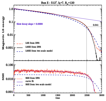
The situation gets more interesting if primordial fields are strong enough, when they are captured and amplified in the formation of a galaxy or cluster, that their energy density is comparble to the turbulent energy density. In this case, naively turbulent diffusion would still lead to its decay. However, itself could be affected and moreover, the nature of the dynamo could change qualitatively in the presence of strong initial fields.
Even more interesting is when the primordial field is helical. It turns out that a large scale helical field is resilient to turbulent diffusion, and only decays on the large resistive time scale (Kemel et al., 2011; Blackman and Subramanian, 2013; Bhat et al., 2014). The reason has again to do with helicity conservation. Suppose we have an initially large scale helical field in the presence of small scale nonhelical turbulence. Then , but is not and contributes to in Eq. (153). This turbulent diffusion then leads to the transfer of helicity to smaller scales, and this buids up until reaches a steady state (bottom panel of Fig. 12). In the presence of the large scale field has a generation term and decays only on the slow resistive timescale. This argument made by Blackman and Subramanian (2013) on the basis of a two scale model, was checked by Bhat et al. (2014) through DNS. The result of one such run, shown in Fig. 12, confirms the picture of initially slow decay of the helical field until it reaches a few percent of the equipartition value, after which it undergoes a rapid decay. Thus if the primordial field were helical, it would seem to be preserved for a resistive times (which is generally longer than the age of the universe) in turbulent galaxies and clusters.
10 Final thoughts
Primordial magnetic fields are important not only because they may explain to some extent the observed fields in the universe, but also because they could provide a window to probe the physics of the early universe. A vast range of mechanisms for their origin have been suggested, but none are as yet natural and or compelling. Theoretical predictions being highly parameter dependent, we have for most part taken a more pragmatic approach, assumed that such a field could be generated in the early Universe and asked how it would evolve and what signals it could leave behind.
The generation during inflation is attractive as it naturally provides the needed coherence; however apart from having to fine tune parameters, there is also the problem of strong coupling. Perhaps the solution to this issue is having theories where some field appears outside the full 4-d action, and then finally goes to renormalize the 4-d distances, rather than the coupling constants. This idea, which was mentioned as a consequence of an evolving higher dimensional scale factor, needs to be better developed. To the author it is also appealing that origin of primordial fields could reflect naturally the influence of evolving extra dimensions. It would also be intriguing if such fields are just a residue left after a proper regularization of the electromagnetic energy momentum tensor during the inflationary era. More work on this idea, which avoids adhoc breaking of conformal invariance, would be of interest.
The idea that the origin of primordial fields is intimately linked to baryogenesis in the simplest extensions of the standard model seems also attractive. One needs of course fairly optimistic assumptions about the amount of energy going into the field at say the EWPT, and it possibly being helical, to get interesting field strengths and coherence scales. However, even very weak fields if they are sufficiently coherent can provide fields in voids, being suggested by high energy gamma ray astronomy.
The linear evolution of large-scale primordial fields is reasonably well understood. The nonlinear evolution, of particularly nonhelical fields has thrown up a surprise; the possibility of inverse cascade of such fields. This unexpected result seems to either reflect an additional conservation law, or the fact that the joint evolution of the velocity and magnetic fields is more complicated than hitherto realized.
We have discussed several signals of the primordial field on the CMB. Currently the Planck data puts upper limits at the few nG level. As the CMB power spectrum goes as the fourth power of the field strength, it may not be possible to easily improve these limits by more than a factor 10 or so. As the magnetic field induced signal is inherently non Gaussian, this would seem to provide a good way to isolate its effects. Clever ideas are also required, combining all the different magnetic field signals to make more progress.
Regarding the effect of primordial fields on structure formation, the work so far has been quite preliminary. The magnetic field is quite a complicated ”entity”, which influences baryonic collapse in an anisotropic fashion, can induce decaying turbulence to heat and ionize the plasma, affect star formation etc. Thus galaxy formation in the presence of strong primordial magnetic fields needs much more work, perhaps using cosmological MHD simulations. This will help to better pin down its effect on reionization and 21 cm signals.
Observations and experiments are the key to progress in any field. In this respect it is heartening to note that the origin of cosmic magnetism is one of the key projects of the SKA. The determination of a large number of accurate rotation measures and its statistical analysis, combined with numerical simulations of structure formation including magnetic fields would be the way to detect and constrain fields in the IGM which could be primordial. Of course the detection of a single case, say in a cluster of fields coherent on Mpc scales, would very much favor a primordial origin. It was also an unexpected bonus that gamma-ray astronomy started probing magnetic fields in voids at the level of G. Even though there could be other explanations for the lack of GeV emission from some of the TeV blazars, the positive detection of such a GeV halo around a TeV blazar, or the time delayed GeV signal, could lead to positive detections of IGM fields; this is an exciting prospect.
Finally, it is appropriate to point out that the study of dynamos and primordial fields are both important and complimentary. Primordial magnetic fields would be interesting as a probe of the physics of the early universe, even if they are not required to seed the dynamo. And dynamos are required to maintain the field in collapsed objects, even if their initial origin were primordial!
References
- (1)
- Adamek et al. (2012) Adamek J, de Rham C and Durrer R 2012 MNRAS 423, 2705–2710.
- Adamek et al. (2011) Adamek J, Durrer R, Fenu E and Vonlanthen M 2011 J. Cosmol. Astropart. Phys. 6, 17.
- Adams et al. (1996) Adams J, Danielsson U H, Grasso D and Rubinstein H 1996 Phys. Lett. B 388, 253–258.
- Agullo et al. (2014) Agullo I, Landete A and Navarro-Salas J 2014 Phys. Rev. D 90(12), 124067.
- Akahori et al. (2014) Akahori T, Gaensler B M and Ryu D 2014 Astrophys. J. 790, 123.
- Akahori and Ryu (2011) Akahori T and Ryu D 2011 Astrophys. J. 738, 134.
- Aoki et al. (2006) Aoki Y, Endrődi G, Fodor Z, Katz S D and Szabó K K 2006 Nature 443, 675–678.
- ATLAS Collaboration (2012) ATLAS Collaboration 2012 Physics Letters B 716(1), 1 – 29.
- Atmjeet et al. (2014) Atmjeet K, Pahwa I, Seshadri T R and Subramanian K 2014 Phys. Rev. D 89(6), 063002.
- Atmjeet et al. (2015) Atmjeet K, Seshadri T R and Subramanian K 2015 Phys. Rev. D 91(10), 103006.
- Atwood et al. (2009) Atwood W B, Abdo A A, Ackermann M, Althouse W, Anderson B, Axelsson M, Baldini L, Ballet J, Band D L, Barbiellini G and et al. 2009 Astrophys. J. 697, 1071–1102.
- Ballardini et al. (2015) Ballardini M, Finelli F and Paoletti D 2015 J. Cosmol. Astropart. Phys. 10, 031.
- Banerjee and Jedamzik (2004) Banerjee R and Jedamzik K 2004 Phys. Rev. D 70(12), 123003.
- Barnaby et al. (2012) Barnaby N, Namba R and Peloso M 2012 Phys. Rev. D 85(12), 123523.
- Barrow et al. (1997) Barrow J D, Ferreira P G and Silk J 1997 Phys. Rev. Lett. 78, 3610–3613.
- Barrow et al. (2007) Barrow J D, Maartens R and Tsagas C G 2007 Phys. Rep. 449, 131–171.
- Barrow et al. (2012) Barrow J D, Tsagas C G and Yamamoto K 2012 Phys. Rev. D 86(2), 023533.
- Bartelmann and Schneider (2001) Bartelmann M and Schneider P 2001 Phys. Rep. 340, 291–472.
- Bartolo et al. (2013) Bartolo N, Matarrese S, Peloso M and Ricciardone A 2013 Phys. Rev. D 87(2), 023504.
- Bassett et al. (2006) Bassett B A, Tsujikawa S and Wands D 2006 Reviews of Modern Physics 78, 537–589.
- Baym et al. (1996) Baym G, Bödeker D and McLerran L 1996 Phys. Rev. D 53, 662–667.
- Baym and Heiselberg (1997) Baym G and Heiselberg H 1997 Phys. Rev. D 56, 5254–5259.
- Bazavov et al. (2014) Bazavov A, Bhattacharya T, DeTar C, Ding H T, Gottlieb S, Gupta R, Hegde P, Heller U M, Karsch F, Laermann E, Levkova L, Mukherjee S, Petreczky P, Schmidt C, Schroeder C, Soltz R A, Soeldner W, Sugar R, Wagner M, Vranas P and HotQCD Collaboration 2014 Phys. Rev. D 90(9), 094503.
- Beck (2001) Beck R 2001 Space Sci. Rev. 99, 243–260.
- Beck and Wielebinski (2013) Beck R and Wielebinski R 2013 p. 641.
- Berger and Field (1984) Berger M A and Field G B 1984 J. Fluid Mech. 147, 133–148.
- Bernet et al. (2008) Bernet M L, Miniati F, Lilly S J, Kronberg P P and Dessauges-Zavadsky M 2008 Nature 454, 302–304.
- Bertone et al. (2006) Bertone S, Vogt C and Enßlin T 2006 MNRAS 370, 319–330.
- Bhat et al. (2014) Bhat P, Blackman E G and Subramanian K 2014 MNRAS 438, 2954–2966.
- Bhat and Subramanian (2013) Bhat P and Subramanian K 2013 MNRAS 429, 2469–2481.
- Bhat et al. (2015) Bhat P, Subramanian K and Brandenburg A 2015 ArXiv e-prints .
- Bi and Davidsen (1997) Bi H and Davidsen A F 1997 Astrophys. J. 479, 523–542.
- BICEP2 Collaboration: et al. (2014) BICEP2 Collaboration:, Ade P A R and et. al. 2014 Physical Review Letters 112(24), 241101.
- BICEP2/Keck and Planck Collaborations: et al. (2015) BICEP2/Keck and Planck Collaborations:, Ade P A R and et. al. 2015 Physical Review Letters 114(10), 101301.
- Biermann (1950) Biermann L 1950 Z. Naturforsch. A 5, 65.
- Biskamp (2003) Biskamp D 2003 Magnetohydrodynamic Turbulence Cambridge University Press Cambridge.
- Biskamp and Müller (1999) Biskamp D and Müller W C 1999 Phys. Rev. Lett. 83, 2195–2198.
- Biskamp and Müller (2000) Biskamp D and Müller W C 2000 Phys. Plasmas 7, 4889–4900.
- Blackman (2014) Blackman E G 2014 Space Sci. Rev. .
- Blackman and Field (2000) Blackman E G and Field G B 2000 Astrophys. J. 534, 984–988.
- Blackman and Field (2002) Blackman E G and Field G B 2002 Phys. Rev. Lett. 89(26), 265007.
- Blackman and Subramanian (2013) Blackman E G and Subramanian K 2013 MNRAS 429, 1398–1406.
- Blasi et al. (1999) Blasi P, Burles S and Olinto A V 1999 Astrophys. J. Lett. 514, L79–L82.
- Bonvin and Caprini (2010) Bonvin C and Caprini C 2010 J. Cosmol. Astropart. Phys. 5, 22.
- Bonvin et al. (2013) Bonvin C, Caprini C and Durrer R 2013 Phys. Rev. D 88(8), 083515.
- Bonvin et al. (2014) Bonvin C, Durrer R and Maartens R 2014 Physical Review Letters 112(19), 191303.
- Boyarsky, Fröhlich and Ruchayskiy (2012) Boyarsky A, Fröhlich J and Ruchayskiy O 2012 Physical Review Letters 108(3), 031301.
- Boyarsky, Ruchayskiy and Shaposhnikov (2012) Boyarsky A, Ruchayskiy O and Shaposhnikov M 2012 Physical Review Letters 109(11), 111602.
- Brandenburg et al. (1996b) Brandenburg A, Enqvist K and Olesen P 1996b Phys. Rev. D 54, 1291–1300.
- Brandenburg et al. (2015) Brandenburg A, Kahniashvili T and Tevzadze A G 2015 Physical Review Letters 114(7), 075001.
- Brandenburg et al. (2012) Brandenburg A, Sokoloff D and Subramanian K 2012 Space Sci. Rev. 169, 123–157.
- Brandenburg and Subramanian (2005a) Brandenburg A and Subramanian K 2005a Phys. Rep. 417, 1–209.
- Broderick et al. (2012) Broderick A E, Chang P and Pfrommer C 2012 Astrophys. J. 752, 22.
- Brown and Crittenden (2005) Brown I and Crittenden R 2005 Phys. Rev. D 72(6), 063002.
- Cai et al. (2010) Cai R G, Hu B and Zhang H B 2010 J. Cosmol. Astropart. Phys. 8, 25.
- Campanelli (2013a) Campanelli L 2013a Physical Review Letters 111(22), 229002.
- Campanelli (2013b) Campanelli L 2013b Physical Review Letters 111(6), 061301.
- Campanelli (2015a) Campanelli L 2015a European Physical Journal C 75, 278.
- Campanelli (2015b) Campanelli L 2015b ArXiv e-prints .
- Campanelli et al. (2004) Campanelli L, Dolgov A D, Giannotti M and Villante F L 2004 Astrophys. J. 616, 1–7.
- Caprini and Durrer (2002) Caprini C and Durrer R 2002 Phys. Rev. D 65(2), 023517.
- Caprini et al. (2004) Caprini C, Durrer R and Kahniashvili T 2004 Phys. Rev. D 69(6), 063006.
- Caprini et al. (2009) Caprini C, Finelli F, Paoletti D and Riotto A 2009 J. Cosmol. Astropart. Phys. 6, 21.
- Caprini and Sorbo (2014) Caprini C and Sorbo L 2014 J. Cosmol. Astropart. Phys. 10, 56.
- Chamandy et al. (2013a) Chamandy L, Subramanian K and Shukurov A 2013a MNRAS 428, 3569–3589.
- Chang et al. (2014) Chang P, Broderick A E, Pfrommer C, Puchwein E, Lamberts A and Shalaby M 2014 Astrophys. J. 797, 110.
- Charbonneau (2014) Charbonneau P 2014 Ann. Rev. Astron. Astrophys. 52, 251–290.
- Chen et al. (2015) Chen W, Chowdhury B D, Ferrer F, Tashiro H and Vachaspati T 2015 MNRAS 450, 3371–3380.
- Chluba, Paoletti, Finelli and Rubiño-Martín (2015) Chluba J, Paoletti D, Finelli F and Rubiño-Martín J A 2015 MNRAS 451, 2244–2250.
- Chluba, Paoletti, Finelli and Rubino-Martin (2015) Chluba J, Paoletti D, Finelli F and Rubino-Martin J A 2015 ArXiv e-prints .
- Cho and Ryu (2009) Cho J and Ryu D 2009 Astrophys. J. Lett. 705, L90–L94.
- Choudhury et al. (2001) Choudhury T R, Srianand R and Padmanabhan T 2001 Astrophys. J. 559, 29–40.
- Christensson et al. (2001) Christensson M, Hindmarsh M and Brandenburg A 2001 Phys. Rev. E 64(5), 056405.
- Clarke et al. (2001) Clarke T E, Kronberg P P and Böhringer H 2001 Astrophys. J. Lett. 547, L111–L114.
- CMS Collaboration (2012) CMS Collaboration 2012 Physics Letters B 716(1), 30 – 61.
- Copi et al. (2008) Copi C J, Ferrer F, Vachaspati T and Achúcarro A 2008 Physical Review Letters 101(17), 171302.
- Cornwall (1997) Cornwall J M 1997 Phys. Rev. D 56, 6146–6154.
- Cowling (1956) Cowling T G 1956 MNRAS 116, 114.
- Croft et al. (2002) Croft R A C, Weinberg D H, Bolte M, Burles S, Hernquist L, Katz N, Kirkman D and Tytler D 2002 Astrophys. J. 581, 20–52.
- Csikor et al. (1998) Csikor F, Fodor Z and Heitger J 1998 Nuclear Physics B Proceedings Supplements 63, 569–571.
- Davidson (2004) Davidson P A 2004 Turbulence : an introduction for scientists and engineers.
- Demozzi et al. (2009) Demozzi V, Mukhanov V and Rubinstein H 2009 J. Cosmol. Astropart. Phys. 8, 25.
- Dermer et al. (2011) Dermer C D, Cavadini M, Razzaque S, Finke J D, Chiang J and Lott B 2011 Astrophys. J. Lett. 733, L21.
- Díaz-Gil et al. (2008a) Díaz-Gil A, García-Bellido J, García Pérez M and González-Arroyo A 2008a Physical Review Letters 100(24), 241301.
- Díaz-Gil et al. (2008b) Díaz-Gil A, García-Bellido J, García Pérez M and González-Arroyo A 2008b Journal of High Energy Physics 7, 43.
- Dodelson (2003) Dodelson S 2003 Modern cosmology.
- Dolgov (1993) Dolgov A D 1993 Phys. Rev. D 48, 2499–2501.
- Durrer (2007) Durrer R 2007 New. Astron. Rev. 51, 275–280.
- Durrer and Caprini (2003) Durrer R and Caprini C 2003 J. Cosmol. Astropart. Phys. 11, 10.
- Durrer et al. (2000) Durrer R, Ferreira P G and Kahniashvili T 2000 Phys. Rev. D 61(4), 043001.
- Durrer et al. (2011) Durrer R, Hollenstein L and Jain R K 2011 J. Cosmol. Astropart. Phys. 3, 37.
- Durrer et al. (2013) Durrer R, Marozzi G and Rinaldi M 2013 Physical Review Letters 111(22), 229001.
- Durrer and Neronov (2013) Durrer R and Neronov A 2013 Astron. Astrophys. Review 21, 62.
- Ellis (1973) Ellis G F R 1973 in E Schatzman, ed., ‘Cargese Lectures in Physics’ Vol. 6 of Cargese Lectures in Physics p. 1.
- Enßlin and Vogt (2006) Enßlin T A and Vogt C 2006 Astron. Astrophys. 453, 447–458.
- Eyink (2011) Eyink G L 2011 Phys. Rev. E 83(5), 056405.
- Eyink et al. (2013) Eyink G, Vishniac E, Lalescu C, Aluie H, Kanov K, Bürger K, Burns R, Meneveau C and Szalay A 2013 Nature 497, 466–469.
- Fan et al. (2006) Fan X, Carilli C L and Keating B 2006 Ann. Rev. Astron. Astrophys. 44, 415–462.
- Faucher-Giguère et al. (2008) Faucher-Giguère C A, Prochaska J X, Lidz A, Hernquist L and Zaldarriaga M 2008 Astrophys. J. 681, 831–855.
- Ferreira et al. (2013) Ferreira R J Z, Jain R K and Sloth M S 2013 J. Cosmol. Astropart. Phys. 10, 4.
- Field and Carroll (2000) Field G B and Carroll S M 2000 Phys. Rev. D 62(10), 103008.
- Finelli et al. (2008) Finelli F, Paci F and Paoletti D 2008 Phys. Rev. D 78(2), 023510.
- Fu et al. (2008) Fu L, Semboloni E, Hoekstra H, Kilbinger M, van Waerbeke L, Tereno I, Mellier Y, Heymans C, Coupon J, Benabed K, Benjamin J, Bertin E, Doré O, Hudson M J, Ilbert O, Maoli R, Marmo C, McCracken H J and Ménard B 2008 Astron. Astrophys. 479, 9–25.
- Fujita and Mukohyama (2012) Fujita T and Mukohyama S 2012 J. Cosmol. Astropart. Phys. 10, 034.
- Fujita et al. (2015) Fujita T, Namba R, Tada Y, Takeda N and Tashiro H 2015 J. Cosmol. Astropart. Phys. 5, 054.
- Fujita and Yokoyama (2013) Fujita T and Yokoyama S 2013 J. Cosmol. Astropart. Phys. 9, 009.
- Furlanetto (2016) Furlanetto S R 2016 in A Mesinger, ed., ‘Astrophysics and Space Science Library’ Vol. 423 of Astrophysics and Space Science Library p. 247.
- Furlanetto and Loeb (2001) Furlanetto S R and Loeb A 2001 Astrophys. J. 556, 619–634.
- Gasperini et al. (1995) Gasperini M, Giovannini M and Veneziano G 1995 Physical Review Letters 75, 3796–3799.
- Giovannini (2000) Giovannini M 2000 Phys. Rev. D 62(12), 123505.
- Giovannini (2008) Giovannini M 2008 in M Gasperini and J Maharana, eds, ‘String Theory and Fundamental Interactions’ Springer Berlin pp. 863–939.
- Giovannini (2010) Giovannini M 2010 Phys. Rev. D 81(12), 127302.
- Giovannini and Kunze (2008) Giovannini M and Kunze K E 2008 Phys. Rev. D 77(6), 063003.
- Gnedin et al. (2000) Gnedin N Y, Ferrara A and Zweibel E G 2000 Astrophys. J. 539, 505–516.
- Gopal and Sethi (2003) Gopal R and Sethi S K 2003 J. Astrophys. Astron. 24, 51–68.
- Gopal and Sethi (2005) Gopal R and Sethi S K 2005 MNRAS 363, 521–528.
- Gorbunov and Rubakov (2011) Gorbunov D S and Rubakov V A 2011 Introduction to the theory of the early universe.
- Govoni and Feretti (2004) Govoni F and Feretti L 2004 Int. J. Mod. Phys. D 13, 1549–1594.
- Grasso and Riotto (1998) Grasso D and Riotto A 1998 Physics Letters B 418, 258–265.
- Grasso and Rubinstein (2001) Grasso D and Rubinstein H R 2001 Phys. Rep. 348, 163–266.
- Grojean et al. (2005) Grojean C, Servant G and Wells J D 2005 Phys. Rev. D 71(3), 036001.
- Harrison (1969) Harrison E R 1969 Nature 224, 1089–1090.
- Hathaway (2010) Hathaway D H 2010 Living Reviews in Solar Physics 7, 1.
- Haugen et al. (2004) Haugen N E, Brandenburg A and Dobler W 2004 Phys. Rev. E 70(1), 016308.
- Himmetoglu et al. (2009) Himmetoglu B, Contaldi C R and Peloso M 2009 Physical Review Letters 102(11), 111301.
- Hinshaw et al. (2013) Hinshaw G, Larson D, Komatsu E, Spergel D N, Bennett C L, Dunkley J, Nolta M R, Halpern M, Hill R S, Odegard N, Page L, Smith K M, Weiland J L, Gold B, Jarosik N, Kogut A, Limon M, Meyer S S, Tucker G S, Wollack E and Wright E L 2013 Astrophys. J. Suppl. 208, 19.
- Hogan (1983) Hogan C J 1983 Physical Review Letters 51, 1488–1491.
- Hu and White (1996) Hu W and White M 1996 Astron. Astrophys. 315, 33–39.
- Hu and White (1997) Hu W and White M 1997 Phys. Rev. D 56, 596–615.
- Huber et al. (2007) Huber S J, Konstandin T, Prokopec T and Schmidt M G 2007 Nuclear Physics A 785, 206–209.
- Jedamzik et al. (1998) Jedamzik K, Katalinić V and Olinto A V 1998 Phys. Rev. D 57, 3264–3284.
- Jedamzik et al. (2000) Jedamzik K, Katalinić V and Olinto A V 2000 Physical Review Letters 85, 700.
- Jedamzik and Sigl (2011) Jedamzik K and Sigl G 2011 Phys. Rev. D 83(10), 103005.
- Johnston-Hollitt et al. (2015) Johnston-Hollitt M, Govoni F, Beck R, Dehghan S, Pratley L, Akahori T, Heald G, Agudo I, Bonafede A, Carretti E, Clarke T, Colafrancesco S, Ensslin T A, Feretti L, Gaensler B, Haverkorn M, Mao S A, Oppermann N, Rudnick L, Scaife A, Schnitzeler D, Stil J, Taylor A R and Vacca V 2015 Advancing Astrophysics with the Square Kilometre Array (AASKA14) p. 92.
- Joyce and Shaposhnikov (1997) Joyce M and Shaposhnikov M 1997 Physical Review Letters 79, 1193–1196.
- Kahniashvili et al. (2014) Kahniashvili T, Maravin Y, Lavrelashvili G and Kosowsky A 2014 Phys. Rev. D 90(8), 083004.
- Kahniashvili and Ratra (2005) Kahniashvili T and Ratra B 2005 Phys. Rev. D 71(10), 103006.
- Kahniashvili et al. (2013) Kahniashvili T, Tevzadze A G, Brandenburg A and Neronov A 2013 Phys. Rev. D 87(8), 083007.
- Kajantie et al. (1996) Kajantie K, Laine M, Rummukainen K and Shaposhnikov M 1996 Physical Review Letters 77, 2887–2890.
- Kandus et al. (2011) Kandus A, Kunze K E and Tsagas C G 2011 Phys. Rep. 505, 1–58.
- Kazantsev (1967) Kazantsev A P 1967 JETP 53, 1807–1813. (English translation: Sov. Phys. JETP, 26, 1031–1034, 1968).
- Keck Array and BICEP2 Collaborations et al. (2016) Keck Array and BICEP2 Collaborations, :, Ade P A R and et. al. 2016 Physical Review Letters 116(3), 031302.
- Kemel et al. (2011) Kemel K, Brandenburg A and Ji H 2011 Phys. Rev. E 84(5), 056407.
- Kempf et al. (2016) Kempf A, Kilian P and Spanier F 2016 Astron. Astrophys. 585, A132.
- Kim et al. (1996) Kim E J, Olinto A V and Rosner R 1996 Astrophys. J. 468, 28.
- Kobayashi and Afshordi (2014) Kobayashi T and Afshordi N 2014 Journal of High Energy Physics 10, 166.
- Kobayashi et al. (2007) Kobayashi T, Maartens R, Shiromizu T and Takahashi K 2007 Phys. Rev. D 75(10), 103501.
- Kojima et al. (2010) Kojima K, Kajino T and Mathews G J 2010 J. Cosmol. Astropart. Phys. 2, 18.
- Kolb and Turner (1990) Kolb E W and Turner M S 1990 The early universe.
- Koopmans et al. (2015) Koopmans L, Pritchard J, Mellema G, Aguirre J, Ahn K, Barkana R, van Bemmel I, Bernardi G, Bonaldi A, Briggs F, de Bruyn A G, Chang T C, Chapman E, Chen X, Ciardi B, Dayal P, Ferrara A, Fialkov A, Fiore F, Ichiki K, Illiev I T, Inoue S, Jelic V, Jones M, Lazio J, Maio U, Majumdar S, Mack K J, Mesinger A, Morales M F, Parsons A, Pen U L, Santos M, Schneider R, Semelin B, de Souza R S, Subrahmanyan R, Takeuchi T, Vedantham H, Wagg J, Webster R, Wyithe S, Datta K K and Trott C 2015 Advancing Astrophysics with the Square Kilometre Array (AASKA14) p. 1.
- Kosowsky et al. (2005) Kosowsky A, Kahniashvili T, Lavrelashvili G and Ratra B 2005 Phys. Rev. D 71(4), 043006.
- Kosowsky and Loeb (1996) Kosowsky A and Loeb A 1996 Astrophys. J. 469, 1.
- Kulsrud (1999) Kulsrud R M 1999 Ann. Rev. Astron. Astrophys. 37, 37–64.
- Kulsrud et al. (1997) Kulsrud R M, Cen R, Ostriker J P and Ryu D 1997 Astrophys. J. 480, 481–491.
- Kunze and Komatsu (2015) Kunze K E and Komatsu E 2015 J. Cosmol. Astropart. Phys. 6, 027.
- Lewis (2004) Lewis A 2004 Phys. Rev. D 70(4), 043011.
-
Linde (2015)
Linde A 2015 in ‘100e Ecole d’Ete de Physique: Post-Planck Cosmology
Les Houches, France, July 8-August 2, 2013’ pp. 231–316.
https://inspirehep.net/record/1280019/files/arXiv:1402.0526.pdf - Linde (1990) Linde A D 1990 Contemporary Concepts in Physics 5.
- Mack et al. (2002) Mack A, Kahniashvili T and Kosowsky A 2002 Phys. Rev. D 65(12), 123004.
- Madau et al. (1997) Madau P, Meiksin A and Rees M J 1997 Astrophys. J. 475, 429–444.
- Martin (2015) Martin J 2015 ArXiv e-prints .
- Martin and Yokoyama (2008) Martin J and Yokoyama J 2008 J. Cosmol. Astropart. Phys. 1, 25.
- Matarrese et al. (2005) Matarrese S, Mollerach S, Notari A and Riotto A 2005 Phys. Rev. D 71(4), 043502.
- Mather et al. (1994) Mather J C, Cheng E S, Cottingham D A, Eplee, Jr. R E, Fixsen D J, Hewagama T, Isaacman R B, Jensen K A, Meyer S S, Noerdlinger P D, Read S M, Rosen L P, Shafer R A, Wright E L, Bennett C L, Boggess N W, Hauser M G, Kelsall T, Moseley, Jr. S H, Silverberg R F, Smoot G F, Weiss R and Wilkinson D T 1994 Astrophys. J. 420, 439–444.
- McDonald et al. (2005) McDonald P, Seljak U, Cen R, Shih D, Weinberg D H, Burles S, Schneider D P, Schlegel D J, Bahcall N A, Briggs J W, Brinkmann J, Fukugita M, Ivezić Ž, Kent S and Vanden Berk D E 2005 Astrophys. J. 635, 761–783.
- Membiela (2014) Membiela F A 2014 Nuclear Physics B 885, 196 – 224.
- Miniati and Elyiv (2013) Miniati F and Elyiv A 2013 Astrophys. J. 770, 54.
- Misner et al. (1973) Misner C W, Thorne K S and Wheeler J A 1973 Gravitation W.H. Freeman and Co. San Francisco.
- Moffatt (1969) Moffatt H K 1969 J. Fluid Mech. 35, 117–129.
- Moffatt (1978) Moffatt H K 1978 Magnetic Field Generation in Electrically Conducting Fluids Cambridge Univ. Press Cambridge.
- Mukhanov (2005) Mukhanov V 2005 Physical Foundations of Cosmology.
- Munshi et al. (2008) Munshi D, Valageas P, van Waerbeke L and Heavens A 2008 Phys. Rep. 462, 67–121.
- Naoz and Narayan (2013) Naoz S and Narayan R 2013 Physical Review Letters 111(5), 051303.
- Narlikar (2002) Narlikar J V 2002 An Introduction to Cosmology Cambridge Univ. Press Cambridge.
- Neronov and Vovk (2010) Neronov A and Vovk I 2010 Science 328, 73–.
- Olesen (2015) Olesen P 2015 ArXiv e-prints .
- Olson (2013) Olson P 2013 Physics Today 66(11), 30.
- Padmanabhan (2002) Padmanabhan T 2002 Theoretical Astrophysics, Volume III: Galaxies and Cosmology Cambridge Univ. Press Cambridge.
- Padmanabhan and Subramanian (1992) Padmanabhan T and Subramanian K 1992 Bull. Astron. Soc. India 20, 1–155.
- Pandey et al. (2015) Pandey K L, Choudhury T R, Sethi S K and Ferrara A 2015 MNRAS 451, 1692–1700.
- Pandey and Sethi (2012) Pandey K L and Sethi S K 2012 Astrophys. J. 748, 27.
- Pandey and Sethi (2013) Pandey K L and Sethi S K 2013 Astrophys. J. 762, 15.
- Paoletti et al. (2009) Paoletti D, Finelli F and Paci F 2009 MNRAS 396, 523–534.
- Peebles (1980) Peebles P J E 1980 The Large-Scale Structure of the Universe Princeton Univ. Press Princeton.
- Peebles (1993) Peebles P J E 1993 Principles of Physical Cosmology.
- Penzias and Wilson (1965) Penzias A A and Wilson R W 1965 Astrophys. J. 142, 419–421.
- Planck Collaboration: XIII et al. (2015) Planck Collaboration: XIII, Ade P A R and et. al. 2015 ArXiv e-prints .
- Planck Collaboration: XIX et al. (2015) Planck Collaboration: XIX, Ade P A R and et. al. 2015 ArXiv e-prints .
- Polarbear Collaboration: et al. (2015) Polarbear Collaboration:, Ade P A R and et. al. 2015 Phys. Rev. D 92, 123509.
- Pouquet et al. (1976) Pouquet A, Frisch U and Leorat J 1976 J. Fluid Mech. 77, 321–354.
- Press and Schechter (1974) Press W H and Schechter P 1974 Astrophys. J. 187, 425–438.
- Pritchard et al. (2015) Pritchard J, Ichiki K, Mesinger A, Metcalf R B, Pourtsidou A, Santos M, Abdalla F B, Chang T C, Chen X, Weller J and Zaroubi S 2015 Advancing Astrophysics with the Square Kilometre Array (AASKA14) p. 12.
- Prunet et al. (1998) Prunet S, Sethi S K, Bouchet F R and Miville-Deschenes M A 1998 Astron. Astrophys. 339, 187–193.
- Pshirkov et al. (2015) Pshirkov M S, Tinyakov P G and Urban F R 2015 ArXiv e-prints .
- Quashnock et al. (1989) Quashnock J M, Loeb A and Spergel D N 1989 Astrophys. J. Lett. 344, L49–L51.
- Ratra (1992) Ratra B 1992 Astrophys. J. Lett. 391, L1–L4.
- Ryu et al. (2012) Ryu D, Schleicher D R G, Treumann R A, Tsagas C G and Widrow L M 2012 Space Sci. Rev. 166, 1–35.
- Schekochihin et al. (2004) Schekochihin A A, Cowley S C, Taylor S F, Maron J L and McWilliams J C 2004 Astrophys. J. 612, 276–307.
- Schleicher et al. (2008) Schleicher D R G, Banerjee R and Klessen R S 2008 Phys. Rev. D 78(8), 083005.
- Schleicher, Banerjee and Klessen (2009) Schleicher D R G, Banerjee R and Klessen R S 2009 Astrophys. J. 692, 236–245.
- Schleicher et al. (2010) Schleicher D R G, Banerjee R, Sur S, Arshakian T G, Klessen R S, Beck R and Spaans M 2010 Astron. Astrophys. 522, A115.
- Schleicher, Galli, Glover, Banerjee, Palla, Schneider and Klessen (2009) Schleicher D R G, Galli D, Glover S C O, Banerjee R, Palla F, Schneider R and Klessen R S 2009 Astrophys. J. 703, 1096–1106.
- Schlickeiser et al. (2012) Schlickeiser R, Ibscher D and Supsar M 2012 Astrophys. J. 758, 102.
- Schober et al. (2013) Schober J, Schleicher D R G and Klessen R S 2013 Astron. Astrophys. 560, A87.
- Schwarz and Stuke (2009) Schwarz D J and Stuke M 2009 J. Cosmol. Astropart. Phys. 11, 25.
- Seljak and Zaldarriaga (1996) Seljak U and Zaldarriaga M 1996 Astrophys. J. 469, 437.
- Semikoz and Sokoloff (2005) Semikoz V B and Sokoloff D 2005 Astron. Astrophys. 433, L53–L56.
- Semikoz et al. (2012) Semikoz V B, Sokoloff D D and Valle J W F 2012 J. Cosmol. Astropart. Phys. 6, 8.
- Seshadri and Subramanian (2001) Seshadri T R and Subramanian K 2001 Phys. Rev. Lett. 87(10), 101301.
- Seshadri and Subramanian (2009) Seshadri T R and Subramanian K 2009 Phys. Rev. Lett. 103(8), 081303.
- Sethi (2005) Sethi S K 2005 MNRAS 363, 818–830.
- Sethi et al. (2008) Sethi S K, Nath B B and Subramanian K 2008 MNRAS 387, 1589–1596.
- Sethi and Subramanian (2005) Sethi S K and Subramanian K 2005 MNRAS 356, 778–788.
- Sethi and Subramanian (2009) Sethi S K and Subramanian K 2009 J. Cosmol. Astropart. Phys. 11, 21.
- Shaposhnikov (1987) Shaposhnikov M E 1987 Nuclear Physics B 287, 757–775.
- Shaw and Lewis (2010) Shaw J R and Lewis A 2010 Phys. Rev. D 81(4), 043517.
- Shiraishi et al. (2010) Shiraishi M, Nitta D, Yokoyama S, Ichiki K and Takahashi K 2010 Phys. Rev. D 82(12), 121302.
- Shiraishi et al. (2011) Shiraishi M, Nitta D, Yokoyama S, Ichiki K and Takahashi K 2011 Phys. Rev. D 83(12), 123003.
- Shiraishi and Sekiguchi (2014) Shiraishi M and Sekiguchi T 2014 Phys. Rev. D 90(10), 103002.
- Shtanov and Sahni (2013) Shtanov Y and Sahni V 2013 J. Cosmol. Astropart. Phys. 1, 8.
- Shu (1992) Shu F H 1992 The physics of astrophysics. Volume II: Gas dynamics.
- Shukurov (2007) Shukurov A 2007 in E Dormy and A. M Soward, eds, ‘Mathematical Aspects of Natural Dynamos’ Chapman & Hall/CRC pp. 313–359.
- Shukurov et al. (2006) Shukurov A, Sokoloff D, Subramanian K and Brandenburg A 2006 Astron. Astrophys. 448, L33–L36.
- Sigl et al. (1997) Sigl G, Olinto A V and Jedamzik K 1997 Phys. Rev. D 55, 4582–4590.
- Silk (1968) Silk J 1968 Astrophys. J. 151, 459.
- Sriramkumar et al. (2015) Sriramkumar L, Atmjeet K and Jain R K 2015 J. Cosmol. Astropart. Phys. 9, 010.
- Stevens and Johnson (2009) Stevens T and Johnson M B 2009 Phys. Rev. D 80(8), 083011.
- Stevens et al. (2012) Stevens T, Johnson M B, Kisslinger L S and Henley E M 2012 Phys. Rev. D 85(6), 063003.
- Stevenson (2010) Stevenson D J 2010 Space Sci. Rev. 152, 651–664.
- Subramanian (1999) Subramanian K 1999 Phys. Rev. Lett. 83, 2957–2960.
- Subramanian (2005) Subramanian K 2005 Current Science 88, 1068–1087.
- Subramanian (2006) Subramanian K 2006 Astron. Nachr. 327, 403.
- Subramanian and Barrow (1998a) Subramanian K and Barrow J D 1998a Phys. Rev. D 58(8), 083502.
- Subramanian and Barrow (1998b) Subramanian K and Barrow J D 1998b Phys. Rev. Lett. 81, 3575–3578.
- Subramanian and Barrow (2002) Subramanian K and Barrow J D 2002 MNRAS 335, L57–L61.
- Subramanian et al. (2003) Subramanian K, Seshadri T R and Barrow J D 2003 MNRAS 344, L31–L35.
- Subramanian (2010) Subramanian K 2010 Astronomische Nachrichten 331, 110.
- Subramanian and Brandenburg (2006) Subramanian K and Brandenburg A 2006 Astrophys. J. Lett. 648, L71–L74.
- Subramanian and Brandenburg (2014) Subramanian K and Brandenburg A 2014 MNRAS 445, 2930–2940.
- Subramanian et al. (1994) Subramanian K, Narasimha D and Chitre S M 1994 MNRAS 271, L15.
- Subramanian et al. (2006) Subramanian K, Shukurov A and Haugen N E L 2006 MNRAS 366, 1437–1454.
- Sur et al. (2010) Sur S, Schleicher D R G, Banerjee R, Federrath C and Klessen R S 2010 Astrophys. J. Lett. 721, L134–L138.
- Sur et al. (2007) Sur S, Shukurov A and Subramanian K 2007 MNRAS 377, 874–882.
- ’t Hooft (1976) ’t Hooft G 1976 Physical Review Letters 37, 8–11.
- Takahashi et al. (2005) Takahashi K, Ichiki K, Ohno H and Hanayama H 2005 Physical Review Letters 95(12), 121301.
- Tashiro et al. (2014) Tashiro H, Chen W, Ferrer F and Vachaspati T 2014 MNRAS 445, L41–L45.
- Tashiro and Sugiyama (2006a) Tashiro H and Sugiyama N 2006a MNRAS 368, 965–970.
- Tashiro and Sugiyama (2006b) Tashiro H and Sugiyama N 2006b MNRAS 372, 1060–1068.
- Tasinato (2015) Tasinato G 2015 J. Cosmol. Astropart. Phys. 3, 040.
- Tavecchio et al. (2011) Tavecchio F, Ghisellini G, Bonnoli G and Foschini L 2011 MNRAS 414, 3566–3576.
- Taylor et al. (2011) Taylor A M, Vovk I and Neronov A 2011 Astron. Astrophys. 529, A144.
- Taylor et al. (2015) Taylor R, Agudo I, Akahori T, Beck R, Gaensler B, Heald G, Johnston-Hollitt M, Langer M, Rudnick L, Scaife A, Schleicher D, Stil J and Ryu D 2015 Advancing Astrophysics with the Square Kilometre Array (AASKA14) p. 113.
- Thorne (1967) Thorne K S 1967 Astrophys. J. 148, 51.
- Trivedi et al. (2012) Trivedi P, Seshadri T R and Subramanian K 2012 Phys. Rev. Lett. 108(23), 231301.
- Trivedi et al. (2010) Trivedi P, Subramanian K and Seshadri T R 2010 Phys. Rev. D 82(12), 123006.
- Trivedi et al. (2014) Trivedi P, Subramanian K and Seshadri T R 2014 Phys. Rev. D 89(4), 043523.
- Tsagas (2005) Tsagas C G 2005 Classical and Quantum Gravity 22, 393–407.
- Tsagas (2014) Tsagas C G 2014 ArXiv e-prints .
- Turner and Widrow (1988) Turner M S and Widrow L M 1988 Phys. Rev. D 37, 2743–2754.
- Turok and Zadrozny (1990) Turok N and Zadrozny J 1990 Physical Review Letters 65, 2331–2334.
- Vachaspati (1991) Vachaspati T 1991 Physics Letters B 265, 258–261.
- Vachaspati (2001) Vachaspati T 2001 Physical Review Letters 87(25), 251302.
- Viel et al. (2004) Viel M, Haehnelt M G and Springel V 2004 MNRAS 354, 684–694.
- Vogt and Enßlin (2005) Vogt C and Enßlin T A 2005 Astron. Astrophys. 434, 67–76.
- Wasserman (1978) Wasserman I 1978 Astrophys. J. 224, 337–343.
- Weinberg (1972) Weinberg S 1972 Gravitation and Cosmology: Principles and Applications of the General Theory of Relativity Wiley New York.
- Weinberg (2008) Weinberg S 2008 Cosmology Oxford Univ. Press Oxford.
- Welter et al. (1984) Welter G L, Perry J J and Kronberg P P 1984 Astrophys. J. 279, 19–39.
- Widrow (2002) Widrow L M 2002 Rev. Mod. Phys. 74, 775–823.
- Widrow et al. (2012) Widrow L M, Ryu D, Schleicher D R G, Subramanian K, Tsagas C G and Treumann R A 2012 Space Sci. Rev. 166, 37–70.
- Yamauchi et al. (2014) Yamauchi D, Fujita T and Mukohyama S 2014 J. Cosmol. Astropart. Phys. 3, 31.
- Yamazaki et al. (2008) Yamazaki D G, Ichiki K, Kajino T and Mathews G J 2008 Phys. Rev. D 77(4), 043005.
- Zeldovich et al. (1990) Zeldovich Ya B, Ruzmaikin A A and Sokoloff D D 1990 The Almighty Chance World Scientific Singapore.
- Zrake (2014) Zrake J 2014 Astrophys. J. Lett. 794, L26.