Gravitational wave signal from primordial magnetic fields in the Pulsar Timing Array frequency band

Abstract

The NANOGrav, Parkes, European, and International Pulsar Timing Array (PTA) Collaborations have reported evidence for a common-spectrum process that can potentially correspond to a stochastic gravitational wave background (SGWB) in the 1–100 nHz frequency range. We consider the scenario in which this signal is produced by magnetohydrodynamic (MHD) turbulence in the early Universe, induced by a nonhelical primordial magnetic field at the energy scale corresponding to the quark confinement phase transition. We perform MHD simulations to study the dynamical evolution of the magnetic field and compute the resulting SGWB. We show that the SGWB output from the simulations can be very well approximated by assuming that the magnetic anisotropic stress is constant in time, over a time interval related to the eddy turnover time. The analytical spectrum that we derive under this assumption features a change of slope at a frequency corresponding to the GW source duration that we confirm with the numerical simulations. We compare the SGWB signal with the PTA data to constrain the temperature scale at which the SGWB is sourced, as well as the amplitude and characteristic scale of the initial magnetic field. We find that the generation temperature is constrained to be in the 1–200 MeV range, the magnetic field amplitude must be $>1$% of the radiation energy density at that time, and the magnetic field characteristic scale is constrained to be $>10$% of the horizon scale. We show that the turbulent decay of this magnetic field will lead to a field at recombination that can help to alleviate the Hubble tension and can be tested by measurements in the voids of the Large Scale Structure with gamma-ray telescopes like the Cherenkov Telescope Array.

I Introduction

The magnetic fields observed today in the voids of the Large Scale Structure (LSS) Neronov and Vovk (2010); Ackermann et al. (2018) could be of primordial origin, generated for example during inflation or primordial phase transitions (for a review, see Ref. Durrer and Neronov (2013), and for a recent update, see Ref. Vachaspati (2021)). Once produced, the magnetic field interacts with the primordial plasma, leading to magnetohydrodynamic (MHD) turbulence due to the high conductivity of the early Universe Ahonen and Enqvist (1996); Brandenburg et al. (1996). The energy-momentum tensor of both the magnetic field and the bulk fluid motions feature a tensor component, which can source a stochastic gravitational wave background (SGWB) (see Ref. Caprini and Figueroa (2018) for a review and references therein). The epoch in the early Universe at which the gravitational wave (GW) production occurs sets the typical frequency of the GW signal. In particular, anisotropic stresses present at the energy scale of the quantum chromodynamics (QCD) phase transition can lead to a GW signal around the nanohertz frequency, in the frequency band of pulsar timing arrays (PTA) Sazhin (1978); Detweiler (1979); Deryagin et al. (1986); Hogan (1986); Witten (1984); Signore and Sanchez (1989); Thorsett and Dewey (1996); Caprini et al. (2010).

Recently, the North American Nanohertz Observatory for Gravitational Waves (NANOGrav) Arzoumanian et al. (2020), followed by the Parkes Pulsar Timing Array (PPTA) Goncharov et al. (2021), the European Pulsar Timing Array (EPTA) Chen et al. (2021), and the International Pulsar Timing Array (IPTA) Antoniadis et al. (2022) Collaborations, have reported the detection of a signal common to all the analyzed pulsars, with very marginal evidence for a quadrupole correlation (following the Hellings-Downs curve), characteristic of a SGWB according to general relativity Hellings and Downs (1983).

Several sources could produce such a signal, in particular a population of merging supermassive black hole binaries Haehnelt (1994); Sesana et al. (2004, 2008). Cosmological sources have also been proposed, including inflationary GWs Vagnozzi (2021); Li et al. (2021a); Kuroyanagi et al. (2021); Sharma (2022); Lazarides et al. (2021); Yi and Zhu ; He et al. , cosmic strings and domain walls Ellis and Lewicki (2021); Blasi et al. (2021); Buchmuller et al. (2020); Samanta and Datta (2021); Bian et al. (2021); Liu et al. (2021); Chiang and Lu (2021); Gorghetto et al. (2021); Blanco-Pillado et al. (2021); Chang and Cui (2022); Lazarides et al. (2021); Buchmuller et al. (2021), primordial black holes Vaskonen and Veermäe (2021); De Luca et al. (2021); Kohri and Terada (2021); Domènech and Pi (2022); Wu et al. (2021), supercooled and dark phase transitions Nakai et al. (2021); Addazi et al. (2021); Ratzinger and Schwaller (2021); Moore and Vecchio (2021), and the QCD phase transition Abe et al. (2021); Arzoumanian et al. (2021); Li et al. (2021b), as well as primordial magnetic fields Neronov et al. (2021); Brandenburg et al. (2021a); Khodadi et al. (2021).

In this work, we study the SGWB generated by MHD turbulence due to the presence of a nonhelical magnetic field at the QCD energy scale and compare it with the common noise measured by NANOGrav, PPTA, EPTA, and IPTA. We refine and extend the analysis of Ref. Neronov et al. (2021), where we used an approximate analytical estimate of the SGWB signal and compared it qualitatively with the NANOGrav measurement. Here, we have conducted numerical MHD simulations to accurately predict the SGWB. We set as initial condition of the simulations a fully developed MHD spectrum for the magnetic field, and zero initial bulk velocity. For the numerical simulations we use the Pencil Code Brandenburg et al. (2021b), as in similar numerical works on the SGWB produced by MHD turbulence during the radiation-dominated era Roper Pol et al. (2020a, b).

We derive a simple analytical formula for the SGWB spectrum that fits the simulation results and widely improves the one given in Ref. Neronov et al. (2021). We then use this formula to compare the MHD-generated SGWB spectrum to the PTA data, including NANOGrav, PPTA, EPTA, and IPTA.

The results we obtain are broadly consistent with those of Ref. Neronov et al. (2021), namely: the PTA observations can be accounted for by GW production from MHD turbulence at the QCD scale, provided i) the temperature is in the range $1{\rm\,MeV}<T_{*}<200{\rm\,MeV}$, ii) the magnetic field characteristic scale is close to the horizon, and it can correspond to the scale of the largest processed eddies if $2{\rm\,MeV}<T_{*}<50{\rm\,MeV}$, and iii) the magnetic field energy density is larger than a few percent of the radiation energy density at $T_{*}$. In particular, we show here that the spectral slope of a SGWB from MHD turbulence at the QCD scale is fully compatible with the PTA constraints.

As already pointed out in Ref. Neronov et al. (2021), a primordial magnetic field with these characteristics has a particularly interesting phenomenology since, besides accounting for the PTA common noise, it could also change the sound horizon at the cosmic microwave background (CMB) epoch, easing the Hubble tension, and explain the magnetic fields observed today in matter structures Jedamzik and Pogosian (2020); Jedamzik et al. (2021); Galli et al. (2022). Such a field is also within the sensitivity range of the next-generation $\gamma$-ray observatory Cherenkov Telescope Array (CTA) Korochkin et al. (2021).

We stress that our results depend on the particular initial conditions that we have chosen, namely a fully developed, nonhelical MHD spectrum for the magnetic field, with no initial bulk velocity. In Refs. Roper Pol et al. (2020b); Kahniashvili et al. (2021); Brandenburg et al. (2021a, c); Roper Pol et al. (2022), similar simulations have been performed using the Pencil Code by inserting an electromotive force to model the initial magnetic field obtaining SGWB spectra that differ from ours, especially at large frequencies, which are of less observational relevance. We have chosen the aforementioned initial conditions for mainly two reasons. First of all, they are conservative: whatever the initial generation mechanism, the magnetic field is expected to enter a phase of fully developed and freely decaying turbulence Ahonen and Enqvist (1996); Brandenburg et al. (1996). Any initial phase of magnetic field growth would increase the GW production Roper Pol et al. (2020b); Kahniashvili et al. (2021); Roper Pol et al. (2022). Secondly, simple initial conditions make it easier to build an analytical description of the simulation outcome. Since we want to model magnetically driven turbulence, we also neglect the presence of initial bulk velocity for simplicity.

The paper is organised as follows. In Sec. II, we analyze GW generation from MHD turbulence. First, we present the equations governing the dynamics of the source and the model for the initial condition (Secs. II.1 and II.2), followed by a derivation of the general expression for the SGWB spectrum, cf. Sec. II.3. We then derive the SGWB spectrum obtained under the assumptions of a constant source (Sec. II.4), and from the MHD simulations (Sec. II.5), and we compare the two results (Sec. II.6). In Sec. III, we adopt the analytical form of the SGWB spectrum, validated with the simulations, and compare it with the PTA measurements, introduced in Sec. III.1, to constrain the magnetic field parameters (Sec. III.2). Furthermore, we consider the effect the magnetic field could have on the CMB at recombination and in the cosmic voids of the LSS (Sec. III.3), and compare our results to those of previous publications, to show the implications of our initial conditions (Sec. III.4). In Sec. IV, we compare the SGWB produced by MHD turbulence with the one produced by supermassive black hole binaries. Finally, we conclude in Sec. V.

We use the $(-\!+\!\!++)$ metric signature and set $c=k_{B}=1$. Magnetic fields are expressed in Lorentz-Heaviside units by setting the vacuum permeability to unity. The Kronecker delta is indicated by $\delta_{ij}$, the $n$-dimensional Dirac delta function by $\delta^{n}(x)$, the Gamma function by $\Gamma(x)$, and the cosine and sine integral functions by ${\rm Ci}(x)$ and ${\rm Si}(x)$, respectively. Fields in Fourier space are indicated by a tilde and we use the Fourier convention $\tilde{B}(\mathchoice{\mbox{\boldmath$\displaystyle k$}}{\mbox{\boldmath$\textstyle k$}}{\mbox{\boldmath$\scriptstyle k$}}{\mbox{\boldmath$\scriptscriptstyle k$}}{})=\int B(\mathchoice{\mbox{\boldmath$\displaystyle x$}}{\mbox{\boldmath$\textstyle x$}}{\mbox{\boldmath$\scriptstyle x$}}{\mbox{\boldmath$\scriptscriptstyle x$}}{})\exp{(i\mathchoice{\mbox{\boldmath$\displaystyle x$}}{\mbox{\boldmath$\textstyle x$}}{\mbox{\boldmath$\scriptstyle x$}}{\mbox{\boldmath$\scriptscriptstyle x$}}{}\cdot\mathchoice{\mbox{\boldmath$\displaystyle k$}}{\mbox{\boldmath$\textstyle k$}}{\mbox{\boldmath$\scriptstyle k$}}{\mbox{\boldmath$\scriptscriptstyle k$}}{})}{\rm\,d}^{3}\mathchoice{\mbox{\boldmath$\displaystyle x$}}{\mbox{\boldmath$\textstyle x$}}{\mbox{\boldmath$\scriptstyle x$}}{\mbox{\boldmath$\scriptscriptstyle x$}}{}$ and $B(\mathchoice{\mbox{\boldmath$\displaystyle x$}}{\mbox{\boldmath$\textstyle x$}}{\mbox{\boldmath$\scriptstyle x$}}{\mbox{\boldmath$\scriptscriptstyle x$}}{})=(2\pi)^{-3}\int\tilde{B}(\mathchoice{\mbox{\boldmath$\displaystyle k$}}{\mbox{\boldmath$\textstyle k$}}{\mbox{\boldmath$\scriptstyle k$}}{\mbox{\boldmath$\scriptscriptstyle k$}}{})\exp{(-i\mathchoice{\mbox{\boldmath$\displaystyle x$}}{\mbox{\boldmath$\textstyle x$}}{\mbox{\boldmath$\scriptstyle x$}}{\mbox{\boldmath$\scriptscriptstyle x$}}{}\cdot\mathchoice{\mbox{\boldmath$\displaystyle k$}}{\mbox{\boldmath$\textstyle k$}}{\mbox{\boldmath$\scriptstyle k$}}{\mbox{\boldmath$\scriptscriptstyle k$}}{})}{\rm\,d}^{3}\mathchoice{\mbox{\boldmath$\displaystyle k$}}{\mbox{\boldmath$\textstyle k$}}{\mbox{\boldmath$\scriptstyle k$}}{\mbox{\boldmath$\scriptscriptstyle k$}}{}$. In Secs. II.1–II.3, space coordinates, time coordinate and (inverse) wave vectors are normalized to the comoving Hubble scale at initial time $\mathcal{H}_{*}^{-1}=t_{*}$, and a subscript $*$ in general denotes quantities at initial time. In Sec. II.4 and following, we restore their dimensions for convenience. Energy densities are normalized by the radiation energy density.

II SGWB spectrum: constant source model and MHD simulations

II.1 Magnetohydrodynamics

In this work, we perform simulations solving the MHD equations and the subsequent GW production with the Pencil Code Brandenburg et al. (2021b). A fully developed stochastic magnetic field $\textstyle B$ is inserted as initial condition of the simulations, while the initial velocity field $\textstyle u$ is zero (though it can be driven by the primordial magnetic field at later times via Lorentz forcing). The MHD equations for a relativistic fluid with $p=\rho/3$ in the Friedmann-Lemaître-Robertson-Walker (FLRW) background metric [$a(t)$ is the scale factor],

$${\rm\,d}s^{2}=a^{2}(t)\left[-{\rm\,d}t^{2}+\delta_{ij}{\rm\,d}x^{i}{\rm\,d}x^{j}\right],$$ (1)

are Brandenburg et al. (1996, 2017a); Durrer and Neronov (2013)

$$\frac{\partial\ln\rho}{\partial t}= \,-\frac{4}{3}\left(\mathchoice{\mbox{\boldmath$\displaystyle\nabla$}}{\mbox{\boldmath$\textstyle\nabla$}}{\mbox{\boldmath$\scriptstyle\nabla$}}{\mbox{\boldmath$\scriptscriptstyle\nabla$}}{}\cdot\mathchoice{\mbox{\boldmath$\displaystyle u$}}{\mbox{\boldmath$\textstyle u$}}{\mbox{\boldmath$\scriptstyle u$}}{\mbox{\boldmath$\scriptscriptstyle u$}}{}+\mathchoice{\mbox{\boldmath$\displaystyle u$}}{\mbox{\boldmath$\textstyle u$}}{\mbox{\boldmath$\scriptstyle u$}}{\mbox{\boldmath$\scriptscriptstyle u$}}{}\cdot\ln\rho\right)$$

$$\,+\frac{1}{\rho}\left[\mathchoice{\mbox{\boldmath$\displaystyle u$}}{\mbox{\boldmath$\textstyle u$}}{\mbox{\boldmath$\scriptstyle u$}}{\mbox{\boldmath$\scriptscriptstyle u$}}{}\cdot\left(\mathchoice{\mbox{\boldmath$\displaystyle J$}}{\mbox{\boldmath$\textstyle J$}}{\mbox{\boldmath$\scriptstyle J$}}{\mbox{\boldmath$\scriptscriptstyle J$}}{}\times\mathchoice{\mbox{\boldmath$\displaystyle B$}}{\mbox{\boldmath$\textstyle B$}}{\mbox{\boldmath$\scriptstyle B$}}{\mbox{\boldmath$\scriptscriptstyle B$}}{}\right)+\eta\mathchoice{\mbox{\boldmath$\displaystyle J$}}{\mbox{\boldmath$\textstyle J$}}{\mbox{\boldmath$\scriptstyle J$}}{\mbox{\boldmath$\scriptscriptstyle J$}}{}^{2}\right],$$ (2)

$$\frac{\partial\mathchoice{\mbox{\boldmath$\displaystyle u$}}{\mbox{\boldmath$\textstyle u$}}{\mbox{\boldmath$\scriptstyle u$}}{\mbox{\boldmath$\scriptscriptstyle u$}}{}}{\partial t}= \,-\mathchoice{\mbox{\boldmath$\displaystyle u$}}{\mbox{\boldmath$\textstyle u$}}{\mbox{\boldmath$\scriptstyle u$}}{\mbox{\boldmath$\scriptscriptstyle u$}}{}\cdot\mathchoice{\mbox{\boldmath$\displaystyle\nabla$}}{\mbox{\boldmath$\textstyle\nabla$}}{\mbox{\boldmath$\scriptstyle\nabla$}}{\mbox{\boldmath$\scriptscriptstyle\nabla$}}{}\mathchoice{\mbox{\boldmath$\displaystyle u$}}{\mbox{\boldmath$\textstyle u$}}{\mbox{\boldmath$\scriptstyle u$}}{\mbox{\boldmath$\scriptscriptstyle u$}}{}+\frac{\mathchoice{\mbox{\boldmath$\displaystyle u$}}{\mbox{\boldmath$\textstyle u$}}{\mbox{\boldmath$\scriptstyle u$}}{\mbox{\boldmath$\scriptscriptstyle u$}}{}}{3}\left(\mathchoice{\mbox{\boldmath$\displaystyle\nabla$}}{\mbox{\boldmath$\textstyle\nabla$}}{\mbox{\boldmath$\scriptstyle\nabla$}}{\mbox{\boldmath$\scriptscriptstyle\nabla$}}{}\cdot\mathchoice{\mbox{\boldmath$\displaystyle u$}}{\mbox{\boldmath$\textstyle u$}}{\mbox{\boldmath$\scriptstyle u$}}{\mbox{\boldmath$\scriptscriptstyle u$}}{}+\mathchoice{\mbox{\boldmath$\displaystyle u$}}{\mbox{\boldmath$\textstyle u$}}{\mbox{\boldmath$\scriptstyle u$}}{\mbox{\boldmath$\scriptscriptstyle u$}}{}\cdot\mathchoice{\mbox{\boldmath$\displaystyle\nabla$}}{\mbox{\boldmath$\textstyle\nabla$}}{\mbox{\boldmath$\scriptstyle\nabla$}}{\mbox{\boldmath$\scriptscriptstyle\nabla$}}{}\ln\rho\right)$$

$$\,-\frac{\mathchoice{\mbox{\boldmath$\displaystyle u$}}{\mbox{\boldmath$\textstyle u$}}{\mbox{\boldmath$\scriptstyle u$}}{\mbox{\boldmath$\scriptscriptstyle u$}}{}}{\rho}\left[\mathchoice{\mbox{\boldmath$\displaystyle u$}}{\mbox{\boldmath$\textstyle u$}}{\mbox{\boldmath$\scriptstyle u$}}{\mbox{\boldmath$\scriptscriptstyle u$}}{}\cdot\left(\mathchoice{\mbox{\boldmath$\displaystyle J$}}{\mbox{\boldmath$\textstyle J$}}{\mbox{\boldmath$\scriptstyle J$}}{\mbox{\boldmath$\scriptscriptstyle J$}}{}\times\mathchoice{\mbox{\boldmath$\displaystyle B$}}{\mbox{\boldmath$\textstyle B$}}{\mbox{\boldmath$\scriptstyle B$}}{\mbox{\boldmath$\scriptscriptstyle B$}}{}\right)+\eta\mathchoice{\mbox{\boldmath$\displaystyle J$}}{\mbox{\boldmath$\textstyle J$}}{\mbox{\boldmath$\scriptstyle J$}}{\mbox{\boldmath$\scriptscriptstyle J$}}{}^{2}\right]-\frac{1}{4}\mathchoice{\mbox{\boldmath$\displaystyle\nabla$}}{\mbox{\boldmath$\textstyle\nabla$}}{\mbox{\boldmath$\scriptstyle\nabla$}}{\mbox{\boldmath$\scriptscriptstyle\nabla$}}{}\ln\rho$$

$$\,+\frac{3}{4\rho}\mathchoice{\mbox{\boldmath$\displaystyle J$}}{\mbox{\boldmath$\textstyle J$}}{\mbox{\boldmath$\scriptstyle J$}}{\mbox{\boldmath$\scriptscriptstyle J$}}{}\times\mathchoice{\mbox{\boldmath$\displaystyle B$}}{\mbox{\boldmath$\textstyle B$}}{\mbox{\boldmath$\scriptstyle B$}}{\mbox{\boldmath$\scriptscriptstyle B$}}{}+\frac{2}{\rho}\mathchoice{\mbox{\boldmath$\displaystyle\nabla$}}{\mbox{\boldmath$\textstyle\nabla$}}{\mbox{\boldmath$\scriptstyle\nabla$}}{\mbox{\boldmath$\scriptscriptstyle\nabla$}}{}\cdot\left(\rho\nu\mathchoice{\mbox{\boldmath$\displaystyle S$}}{\mbox{\boldmath$\textstyle S$}}{\mbox{\boldmath$\scriptstyle S$}}{\mbox{\boldmath$\scriptscriptstyle S$}}{}\right),$$ (3)

$$\frac{\partial\mathchoice{\mbox{\boldmath$\displaystyle B$}}{\mbox{\boldmath$\textstyle B$}}{\mbox{\boldmath$\scriptstyle B$}}{\mbox{\boldmath$\scriptscriptstyle B$}}{}}{\partial t}= \,\mathchoice{\mbox{\boldmath$\displaystyle\nabla$}}{\mbox{\boldmath$\textstyle\nabla$}}{\mbox{\boldmath$\scriptstyle\nabla$}}{\mbox{\boldmath$\scriptscriptstyle\nabla$}}{}\times\left(\mathchoice{\mbox{\boldmath$\displaystyle u$}}{\mbox{\boldmath$\textstyle u$}}{\mbox{\boldmath$\scriptstyle u$}}{\mbox{\boldmath$\scriptscriptstyle u$}}{}\times\mathchoice{\mbox{\boldmath$\displaystyle B$}}{\mbox{\boldmath$\textstyle B$}}{\mbox{\boldmath$\scriptstyle B$}}{\mbox{\boldmath$\scriptscriptstyle B$}}{}-\eta\mathchoice{\mbox{\boldmath$\displaystyle J$}}{\mbox{\boldmath$\textstyle J$}}{\mbox{\boldmath$\scriptstyle J$}}{\mbox{\boldmath$\scriptscriptstyle J$}}{}\right),\quad\mathchoice{\mbox{\boldmath$\displaystyle J$}}{\mbox{\boldmath$\textstyle J$}}{\mbox{\boldmath$\scriptstyle J$}}{\mbox{\boldmath$\scriptscriptstyle J$}}{}=\mathchoice{\mbox{\boldmath$\displaystyle\nabla$}}{\mbox{\boldmath$\textstyle\nabla$}}{\mbox{\boldmath$\scriptstyle\nabla$}}{\mbox{\boldmath$\scriptscriptstyle\nabla$}}{}\times\mathchoice{\mbox{\boldmath$\displaystyle B$}}{\mbox{\boldmath$\textstyle B$}}{\mbox{\boldmath$\scriptstyle B$}}{\mbox{\boldmath$\scriptscriptstyle B$}}{},$$ (4)

where $\rho$ is the energy density, $\textstyle J$ the current density, $S_{ij}={\textstyle{1\over 2}}(u_{i,j}+u_{j,i})-{\textstyle{1\over 3}}\mathchoice{\mbox{\boldmath$\displaystyle\nabla$}}{\mbox{\boldmath$\textstyle\nabla$}}{\mbox{\boldmath$\scriptstyle\nabla$}}{\mbox{\boldmath$\scriptscriptstyle\nabla$}}{}\cdot\mathchoice{\mbox{\boldmath$\displaystyle u$}}{\mbox{\boldmath$\textstyle u$}}{\mbox{\boldmath$\scriptstyle u$}}{\mbox{\boldmath$\scriptscriptstyle u$}}{}$ the rate-of-strain tensor, $\nu$ the kinematic viscosity, and $\eta$ the magnetic diffusivity. The space coordinates are comoving with the expansion of the Universe and normalized by the comoving Hubble radius ${\cal H}_{*}^{-1}$; $t$ denotes conformal time, also normalized by ${\cal H}_{*}^{-1}$. All MHD fields are comoving and normalized by the radiation energy density, ${\cal E}_{\rm rad}=3{\cal H}^{2}/8\pi Ga^{2}$ (where $G$ is the gravitation constant) Brandenburg et al. (1996, 2017a); Roper Pol et al. (2020b, a).

II.2 Magnetic field

We model the (normalized) magnetic field as a stochastic nonhelical field, statistically homogeneous, isotropic and Gaussian. Hence, the two-point autocorrelation function is sufficient to describe it statistically due to the Isserlis theorem Isserlis (1916); Monin and Yaglom (1975). At unequal times, the autocorrelation takes the form

$$\langle\tilde{B}_{i}^{*}(\mathchoice{\mbox{\boldmath$\displaystyle k$}}{\mbox{\boldmath$\textstyle k$}}{\mbox{\boldmath$\scriptstyle k$}}{\mbox{\boldmath$\scriptscriptstyle k$}}{},t_{1})\,\tilde{B}_{j}(\mathchoice{\mbox{\boldmath$\displaystyle k$}}{\mbox{\boldmath$\textstyle k$}}{\mbox{\boldmath$\scriptstyle k$}}{\mbox{\boldmath$\scriptscriptstyle k$}}{}^{\prime},t_{2})\rangle=$$

$$(2\pi)^{6}\delta^{3}(\mathchoice{\mbox{\boldmath$\displaystyle k$}}{\mbox{\boldmath$\textstyle k$}}{\mbox{\boldmath$\scriptstyle k$}}{\mbox{\boldmath$\scriptscriptstyle k$}}{}- \,\mathchoice{\mbox{\boldmath$\displaystyle k$}}{\mbox{\boldmath$\textstyle k$}}{\mbox{\boldmath$\scriptstyle k$}}{\mbox{\boldmath$\scriptscriptstyle k$}}{}^{\prime})P_{ij}(\mathchoice{\mbox{\boldmath$\displaystyle k$}}{\mbox{\boldmath$\textstyle k$}}{\mbox{\boldmath$\scriptstyle k$}}{\mbox{\boldmath$\scriptscriptstyle k$}}{})\frac{E_{\rm M}(k,t_{1},t_{2})}{4\pi k^{2}},$$ (5)

where $E_{\rm M}(k,t_{1},t_{2})$ is the unequal-time correlator (UETC), reducing, at equal time $t_{2}=t_{1}$, to the normalized magnetic field energy density spectrum $E_{\rm M}(k,t_{1})$. Furthermore, $P_{ij}=\delta_{ij}-\hat{k}_{i}\hat{k}_{j}$ is the projection tensor, with $\hat{\mathchoice{\mbox{\boldmath$\displaystyle k$}}{\mbox{\boldmath$\textstyle k$}}{\mbox{\boldmath$\scriptstyle k$}}{\mbox{\boldmath$\scriptscriptstyle k$}}}{}$ indicating the unit wave vector $\hat{\mathchoice{\mbox{\boldmath$\displaystyle k$}}{\mbox{\boldmath$\textstyle k$}}{\mbox{\boldmath$\scriptstyle k$}}{\mbox{\boldmath$\scriptscriptstyle k$}}}{}=\mathchoice{\mbox{\boldmath$\displaystyle k$}}{\mbox{\boldmath$\textstyle k$}}{\mbox{\boldmath$\scriptstyle k$}}{\mbox{\boldmath$\scriptscriptstyle k$}}{}/|\mathchoice{\mbox{\boldmath$\displaystyle k$}}{\mbox{\boldmath$\textstyle k$}}{\mbox{\boldmath$\scriptstyle k$}}{\mbox{\boldmath$\scriptscriptstyle k$}}{}|$. The angle brackets indicate ensemble average over stochastic realizations, which can be approximated by a volume average in homogeneous turbulence Monin and Yaglom (1975).

At the initial time $t_{*}$, we assume that the magnetic energy spectrum $E_{\rm M}(k,t_{*})$ is characterized by a Batchelor spectrum at large scales and a Kolmogorov spectrum at small scales, peaking at the characteristic scale $k_{*}=2\pi/l_{*}$. Magnetic fields produced by causal processes, e.g., during cosmological phase transitions, feature a finite correlation length, which leads to a Batchelor magnetic spectrum in the limit $k\rightarrow 0$ Monin and Yaglom (1975); Durrer and Caprini (2003). The Kolmogorov-type $k^{-5/3}$ spectrum is found and well established in purely hydrodynamic turbulence Kolmogorov (1941). In general MHD, different models have been proposed, e.g., Iroshnikov-Kraichnan $k^{-3/2}$ Kraichnan (1965); Iroshnikov (1964), Goldreich-Sridhar $k^{-5/3}$ Goldreich and Sridhar (1995), weak turbulence $k^{-2}$ Ng and Bhattacharjee (1997), and Boldyrev $k^{-3/2}$ Boldyrev (2006). Simulations of MHD turbulence in this context seem to indicate the development of a turbulent spectrum with a $k^{-5/3}$ scaling Christensson et al. (2001); Müller and Biskamp (2000); Kahniashvili et al. (2013); Brandenburg et al. (2015); Brandenburg and Kahniashvili (2017); Brandenburg et al. (2017a). We therefore adopt the following spectral shape:

$$E_{\rm M}(k,t_{*})= \,(1+\mathcal{D})^{1/\alpha}E_{\rm M}^{*}$$

$$\times \,\frac{(k/k_{\ast})^{4}}{\left[1+\mathcal{D}(k/k_{\ast})^{\alpha(4+5/3)}\right]^{1/\alpha}},$$ (6)

where $E_{\rm M}^{*}=E_{\rm M}(k_{\ast},t_{*})$ denotes the magnetic amplitude at the peak $k_{*}$ and at initial time, the parameter $\mathcal{D}=12/5$ is tuned so that the spectrum peaks at $k=k_{\ast}$, and the parameter $\alpha$ indicates the smoothness of the transition between the Batchelor ($\sim\!k^{4}$) and Kolmogorov ($\sim\!k^{-5/3}$) scalings around the spectral peak: we set it to $\alpha=2$ based on previous fits of simulated spectra Brandenburg et al. (2017a). Note that $E_{\rm M}^{*}$ is the maximal value of the magnetic amplitude, since we consider decaying MHD turbulence.

The simulations are initialized with the magnetic field Brandenburg et al. (2017a); Roper Pol et al. (2020b, 2022)

$$\tilde{B}_{i}(\mathchoice{\mbox{\boldmath$\displaystyle k$}}{\mbox{\boldmath$\textstyle k$}}{\mbox{\boldmath$\scriptstyle k$}}{\mbox{\boldmath$\scriptscriptstyle k$}}{},t_{*})=P_{ij}(\mathchoice{\mbox{\boldmath$\displaystyle k$}}{\mbox{\boldmath$\textstyle k$}}{\mbox{\boldmath$\scriptstyle k$}}{\mbox{\boldmath$\scriptscriptstyle k$}}{})g_{j}(\mathchoice{\mbox{\boldmath$\displaystyle k$}}{\mbox{\boldmath$\textstyle k$}}{\mbox{\boldmath$\scriptstyle k$}}{\mbox{\boldmath$\scriptscriptstyle k$}}{})g_{0}(k),$$ (7)

where $g_{j}(\mathchoice{\mbox{\boldmath$\displaystyle k$}}{\mbox{\boldmath$\textstyle k$}}{\mbox{\boldmath$\scriptstyle k$}}{\mbox{\boldmath$\scriptscriptstyle k$}}{})$ is the Fourier transform of a $\delta$-correlated vector field in three dimensions with Gaussian fluctuations, i.e., $g_{i}(\mathchoice{\mbox{\boldmath$\displaystyle x$}}{\mbox{\boldmath$\textstyle x$}}{\mbox{\boldmath$\scriptstyle x$}}{\mbox{\boldmath$\scriptscriptstyle x$}}{})g_{j}(\mathchoice{\mbox{\boldmath$\displaystyle x$}}{\mbox{\boldmath$\textstyle x$}}{\mbox{\boldmath$\scriptstyle x$}}{\mbox{\boldmath$\scriptscriptstyle x$}}{}^{\prime})=\delta_{ij}\delta^{3}(\mathchoice{\mbox{\boldmath$\displaystyle x$}}{\mbox{\boldmath$\textstyle x$}}{\mbox{\boldmath$\scriptstyle x$}}{\mbox{\boldmath$\scriptscriptstyle x$}}{}-\mathchoice{\mbox{\boldmath$\displaystyle x$}}{\mbox{\boldmath$\textstyle x$}}{\mbox{\boldmath$\scriptstyle x$}}{\mbox{\boldmath$\scriptscriptstyle x$}}{}^{\prime})$, and $g_{0}(k)=\sqrt{E_{\rm M}(k,t_{*})}/k$ corresponds to the magnetic spectral shape defined in Eq. (6). We therefore assume that the MHD-processed magnetic spectrum is already established when the GW generation starts. The simulations output the GW generation by the subsequent magnetic turbulent decay, by solving the full MHD system of Eqs. (2)–(4). The initial amplitude $E_{\rm M}^{*}$ and the position of the spectral peak $k_{\ast}$ are the input parameters of the numerical simulations in Sec. II.5.

The total normalized magnetic energy density is $\Omega_{\rm M}(t)={\cal E}_{\rm M}(t)/{\cal E}_{\rm rad}(t)={\textstyle{1\over 2}}\langle{\bf B}^{2}({\mathchoice{\mbox{\boldmath$\displaystyle x$}}{\mbox{\boldmath$\textstyle x$}}{\mbox{\boldmath$\scriptstyle x$}}{\mbox{\boldmath$\scriptscriptstyle x$}}{}},t)\rangle$. Using Eqs. (5) and (6), at initial time, this becomes

$$\Omega_{\rm M}^{*}=\Omega_{\rm M}(t_{*})= \,\int_{0}^{\infty}E_{\rm M}(k,t_{*}){\rm\,d}k$$

$$= \,k_{\ast}E_{\rm M}^{*}{\cal A}(\alpha),$$ (8)

with

$${\cal A}(\alpha=2)= \frac{3^{19\over 34}\,\Gamma\bigl{[}\textstyle{1\over 17}\bigr{]}\,\Gamma\bigl{[}\textstyle{15\over 34}\bigr{]}}{5^{1\over 17}\,2^{32\over 17}\sqrt{17\pi}}\approx 2.064.$$ (9)

The (normalized) magnetic stress tensor components are $T_{ij}(\mathchoice{\mbox{\boldmath$\displaystyle x$}}{\mbox{\boldmath$\textstyle x$}}{\mbox{\boldmath$\scriptstyle x$}}{\mbox{\boldmath$\scriptscriptstyle x$}}{},t)=-B_{i}(\mathchoice{\mbox{\boldmath$\displaystyle x$}}{\mbox{\boldmath$\textstyle x$}}{\mbox{\boldmath$\scriptstyle x$}}{\mbox{\boldmath$\scriptscriptstyle x$}}{},t)B_{j}(\mathchoice{\mbox{\boldmath$\displaystyle x$}}{\mbox{\boldmath$\textstyle x$}}{\mbox{\boldmath$\scriptstyle x$}}{\mbox{\boldmath$\scriptscriptstyle x$}}{},t)+{\textstyle{1\over 2}}\delta_{ij}\mathchoice{\mbox{\boldmath$\displaystyle B$}}{\mbox{\boldmath$\textstyle B$}}{\mbox{\boldmath$\scriptstyle B$}}{\mbox{\boldmath$\scriptscriptstyle B$}}{}^{2}(\mathchoice{\mbox{\boldmath$\displaystyle x$}}{\mbox{\boldmath$\textstyle x$}}{\mbox{\boldmath$\scriptstyle x$}}{\mbox{\boldmath$\scriptscriptstyle x$}}{},t)$, and the traceless and transverse (TT) projection of the stress tensor in Fourier space is $\tilde{\Pi}_{ij}(\mathchoice{\mbox{\boldmath$\displaystyle k$}}{\mbox{\boldmath$\textstyle k$}}{\mbox{\boldmath$\scriptstyle k$}}{\mbox{\boldmath$\scriptscriptstyle k$}}{},t)=\tilde{T}_{ij}^{\rm TT}(\mathchoice{\mbox{\boldmath$\displaystyle k$}}{\mbox{\boldmath$\textstyle k$}}{\mbox{\boldmath$\scriptstyle k$}}{\mbox{\boldmath$\scriptscriptstyle k$}}{},t)=\Lambda_{ijlm}(\hat{\mathchoice{\mbox{\boldmath$\displaystyle k$}}{\mbox{\boldmath$\textstyle k$}}{\mbox{\boldmath$\scriptstyle k$}}{\mbox{\boldmath$\scriptscriptstyle k$}}}{})\tilde{T}_{lm}(\mathchoice{\mbox{\boldmath$\displaystyle k$}}{\mbox{\boldmath$\textstyle k$}}{\mbox{\boldmath$\scriptstyle k$}}{\mbox{\boldmath$\scriptscriptstyle k$}}{},t)$, with $\Lambda_{ijlm}=P_{il}P_{jm}-{\textstyle{1\over 2}}P_{ij}P_{lm}$. The TT-projected stress $\Pi_{ij}$ sources the GWs. As $B_{i}(\mathchoice{\mbox{\boldmath$\displaystyle x$}}{\mbox{\boldmath$\textstyle x$}}{\mbox{\boldmath$\scriptstyle x$}}{\mbox{\boldmath$\scriptscriptstyle x$}}{},t)$, $\Pi_{ij}$ is also a random variable: the GW production can therefore be described statistically using the UETC of the tensor stress $E_{\Pi}(k,t_{1},t_{2})$, defined in analogy with Eq. (5), as

$$\langle\Pi_{ij}({\mathchoice{\mbox{\boldmath$\displaystyle x$}}{\mbox{\boldmath$\textstyle x$}}{\mbox{\boldmath$\scriptstyle x$}}{\mbox{\boldmath$\scriptscriptstyle x$}}{}},t_{1}) \,\Pi_{ij}({\mathchoice{\mbox{\boldmath$\displaystyle x$}}{\mbox{\boldmath$\textstyle x$}}{\mbox{\boldmath$\scriptstyle x$}}{\mbox{\boldmath$\scriptscriptstyle x$}}{}},t_{2})\rangle=$$

$$\,\int_{0}^{\infty}E_{\Pi}(k,t_{1},t_{2}){\rm\,d}k.$$ (10)

For a Gaussian magnetic field (as the one with which we initialize the simulations), the UETC is Caprini et al. (2009a)

$$E_{\Pi}(k,t_{1},t_{2}) \,={k^{2}\over 4\pi}\int\frac{{\rm\,d}^{3}\mathchoice{\mbox{\boldmath$\displaystyle p$}}{\mbox{\boldmath$\textstyle p$}}{\mbox{\boldmath$\scriptstyle p$}}{\mbox{\boldmath$\scriptscriptstyle p$}}{}}{p^{2}|{\mathchoice{\mbox{\boldmath$\displaystyle k$}}{\mbox{\boldmath$\textstyle k$}}{\mbox{\boldmath$\scriptstyle k$}}{\mbox{\boldmath$\scriptscriptstyle k$}}{}-\mathchoice{\mbox{\boldmath$\displaystyle p$}}{\mbox{\boldmath$\textstyle p$}}{\mbox{\boldmath$\scriptstyle p$}}{\mbox{\boldmath$\scriptscriptstyle p$}}{}}|^{2}}E_{\rm M}(p,t_{1},t_{2})$$

$$\,\times E_{\rm M}(|{\mathchoice{\mbox{\boldmath$\displaystyle k$}}{\mbox{\boldmath$\textstyle k$}}{\mbox{\boldmath$\scriptstyle k$}}{\mbox{\boldmath$\scriptscriptstyle k$}}{}-\mathchoice{\mbox{\boldmath$\displaystyle p$}}{\mbox{\boldmath$\textstyle p$}}{\mbox{\boldmath$\scriptstyle p$}}{\mbox{\boldmath$\scriptscriptstyle p$}}{}}|,t_{1},t_{2})\Bigl{(}1+(\hat{\mathchoice{\mbox{\boldmath$\displaystyle k$}}{\mbox{\boldmath$\textstyle k$}}{\mbox{\boldmath$\scriptstyle k$}}{\mbox{\boldmath$\scriptscriptstyle k$}}}{}\cdot\hat{\mathchoice{\mbox{\boldmath$\displaystyle p$}}{\mbox{\boldmath$\textstyle p$}}{\mbox{\boldmath$\scriptstyle p$}}{\mbox{\boldmath$\scriptscriptstyle p$}}}{})^{2}\Bigr{)}$$

$$\,\times\Bigl{(}1+(\hat{\mathchoice{\mbox{\boldmath$\displaystyle k$}}{\mbox{\boldmath$\textstyle k$}}{\mbox{\boldmath$\scriptstyle k$}}{\mbox{\boldmath$\scriptscriptstyle k$}}}{}\cdot\widehat{\mathchoice{\mbox{\boldmath$\displaystyle k$}}{\mbox{\boldmath$\textstyle k$}}{\mbox{\boldmath$\scriptstyle k$}}{\mbox{\boldmath$\scriptscriptstyle k$}}{}-\mathchoice{\mbox{\boldmath$\displaystyle p$}}{\mbox{\boldmath$\textstyle p$}}{\mbox{\boldmath$\scriptstyle p$}}{\mbox{\boldmath$\scriptscriptstyle p$}}{}})^{2}\Bigr{)}.$$ (11)

II.3 Gravitational wave production

GWs are defined as the metric tensor perturbations $\bar{h}_{ij}$ over the FLRW metric, defined in Eq. (1),

$${\rm\,d}s^{2}=a^{2}(t)\,\left[-{\rm\,d}t^{2}+(\delta_{ij}+\bar{h}_{ij})\,{\rm\,d}x^{i}{\rm\,d}x^{j}\right]\,.$$ (12)

We restrict to the radiation era and, as previously, space and time are normalized with ${\cal H}_{*}^{-1}$. We assume that the scale factor evolves linearly with conformal time during the GW sourcing and normalize it such that $a=t$ with $a_{*}=1$ Roper Pol et al. (2020a). The wave equation in the radiation era for the scaled variable $h_{ij}=a\bar{h}_{ij}$ Grishchuk (1974), following the normalization of Refs. Roper Pol et al. (2020a, b), becomes

$$\Bigl{(}\partial_{t}^{2}+\mathchoice{\mbox{\boldmath$\displaystyle k$}}{\mbox{\boldmath$\textstyle k$}}{\mbox{\boldmath$\scriptstyle k$}}{\mbox{\boldmath$\scriptscriptstyle k$}}{}^{2}\Bigr{)}\,\tilde{h}_{ij}(\mathchoice{\mbox{\boldmath$\displaystyle k$}}{\mbox{\boldmath$\textstyle k$}}{\mbox{\boldmath$\scriptstyle k$}}{\mbox{\boldmath$\scriptscriptstyle k$}}{},t)=\frac{6\,\tilde{\Pi}_{ij}(\mathchoice{\mbox{\boldmath$\displaystyle k$}}{\mbox{\boldmath$\textstyle k$}}{\mbox{\boldmath$\scriptstyle k$}}{\mbox{\boldmath$\scriptscriptstyle k$}}{},t)}{t}\,,$$ (13)

where $k$ is the wave number normalized with ${\cal H}_{*}$ and the tensor stress sourcing the GWs is defined above Eq. (10). Assuming that the source is acting until a finite time $t_{\rm fin}$, the solution to Eq. (13) with initial conditions $\tilde{h}_{ij}(\mathchoice{\mbox{\boldmath$\displaystyle k$}}{\mbox{\boldmath$\textstyle k$}}{\mbox{\boldmath$\scriptstyle k$}}{\mbox{\boldmath$\scriptscriptstyle k$}}{},t_{*})=\partial_{t}\tilde{h}_{ij}(\mathchoice{\mbox{\boldmath$\displaystyle k$}}{\mbox{\boldmath$\textstyle k$}}{\mbox{\boldmath$\scriptstyle k$}}{\mbox{\boldmath$\scriptscriptstyle k$}}{},t_{*})=0$, matched with the homogeneous solution at $t_{\rm fin}$, describes a freely propagating wave at times $t>t_{\rm fin}$:

$$\tilde{h}_{ij}(\mathchoice{\mbox{\boldmath$\displaystyle k$}}{\mbox{\boldmath$\textstyle k$}}{\mbox{\boldmath$\scriptstyle k$}}{\mbox{\boldmath$\scriptscriptstyle k$}}{},t)=\frac{6}{k}\int_{t_{*}}^{t_{\rm fin}}\frac{\tilde{\Pi}_{ij}(\mathchoice{\mbox{\boldmath$\displaystyle k$}}{\mbox{\boldmath$\textstyle k$}}{\mbox{\boldmath$\scriptstyle k$}}{\mbox{\boldmath$\scriptscriptstyle k$}}{},t_{1})}{t_{1}}\sin k(t-t_{1}){\rm\,d}t_{1}.$$ (14)

The GW energy density, normalized to the radiation energy density ${\cal E}_{\rm rad}$, is

$$\Omega_{\rm GW}(t)= \,\frac{1}{12}\,\big{\langle}\big{(}\partial_{t}h_{ij}({\bf x},t)-h_{ij}({\bf x},t)/t\big{)}^{2}\big{\rangle}$$

$$= \,\int_{-\infty}^{\infty}\Omega_{\rm GW}(k,t){\rm\,d}\ln k,$$ (15)

where $\Omega_{\rm GW}(k,t)$ denotes the normalized logarithmic GW energy density spectrum. Fourier transforming Eq. (15) and inserting solution (14), it becomes, at times $t>t_{\rm fin}$,

$$\Omega_{\rm GW}(k,t) \,=3\,k\int_{t_{*}}^{t_{\rm fin}}\frac{dt_{1}}{t_{1}}\int_{t_{*}}^{t_{\rm fin}}\frac{dt_{2}}{t_{2}}$$

$$\,\times E_{\Pi}(k,t_{1},t_{2})\,S(k,t,t_{1},t_{2}),$$ (16)

with

$$S(k,t,t_{1},t_{2})\approx \,\cos k(t-t_{1})\cos k(t-t_{2}).$$ (17)

In the above equation, we have omitted the terms proportional to $1/(kt)$ that appear due to the $h_{ij}/t$ term in Eq. (15) since, at present time, all relevant wave numbers of signals produced in the early Universe are inside the horizon $kt\gg 1$.

II.4 Analytical GW spectrum for constant-in-time stress

The characteristic time of the magnetic field decay in a turbulent MHD cascade is the eddy turnover time $\delta t_{\rm e}=t_{\rm e}-t_{*}=(v_{\rm A}k_{\ast})^{-1}$, where $v_{\rm A}=\sqrt{{\textstyle{3\over 2}}\Omega_{\rm M}^{*}}$ is the Alfvén speed at initial time and $k_{*}$ the initial characteristic wave number.

The GW sourcing, on the other hand, occurs on a characteristic time interval $\delta t=t-t_{*}\sim 1/k$ for a given GW wave number $k$, as can be inferred from the Green function of the wave equation (14), which has period $2\pi/k$. Indeed, recent simulations of GW production by MHD turbulence have shown that each mode $k$ of the GW spectrum in the simulation box reached a stationary amplitude after an initial growth period lasting $\delta t\sim 1/k$ Roper Pol et al. (2020b, 2022). Since the GW spectrum is expected to peak around $k_{*}$, the GW sourcing is faster than the magnetic field decay for all wave numbers satisfying $k>v_{\rm A}k_{*}$, i.e., around and above the GW spectrum peak. Correspondingly, the simulations have also shown that the total GW energy density, which is dominated by the spectral amplitude at the peak, enters a stationary regime shortly after the time interval $\delta t_{\rm GW}\approx 1/k_{\ast}$ Roper Pol et al. (2020b, 2022). Comparing the latter to the eddy turnover time gives, by causality, $\delta t_{\rm GW}/\delta t_{\rm e}=v_{\rm A}\lesssim 1$. More precisely, one has $v_{\rm A}\lesssim 0.4$, since big bang nucleosynthesis (BBN) limits $\Omega_{\rm M}^{*}\lesssim 0.1$ Shvartsman (1969); Grasso and Rubinstein (1996); Kahniashvili et al. (2011).

Since the dynamical evolution of GW production is faster than that of the magnetic field for all relevant wave numbers, we can assume, as a first approximation, that the magnetic stresses in Eq. (16) are constant in time. The role of $t_{\rm fin}$ in Eq. (16) becomes then to cut off the constant source, inserting an effective source duration $\delta t_{\rm fin}=t_{\rm fin}-t_{*}$. The latter is expected to be related to the characteristic time of the magnetic field decay, $\delta t_{\rm fin}\gtrsim\delta t_{\rm e}$. As we shall see, the effective source duration $\delta t_{\rm fin}$ introduces a feature in the SGWB spectrum, i.e., a change of spectral slope between the wave numbers for which the GW production is faster than the source decay $k\gtrsim 1/\delta t_{\rm e}\gtrsim 1/\delta t_{\rm fin}$ and those for which the GW production is slower $k<1/\delta t_{\rm fin}$.

In the following, we first present the analytic calculation of the GW spectrum under the assumption that the magnetic stress is constant in time up to $t_{\rm fin}$. We then revise the qualitative analysis of Ref. Neronov et al. (2021) using the more accurate prediction for the GW spectrum derived previously. In the next subsection (Sec. II.5), we discuss the results of the simulations. We then show, in Sec. II.6, that the constant source model approximates very well the GW spectra output from the simulations and use the latter to compute the specific value of the parameter $\delta t_{\rm fin}$ and infer empirically its relation to $\delta t_{\rm e}$.

II.4.1 Analytical GW spectrum

If we assume that the stress is constant in time, Eq. (16) can be easily integrated to find (note that from this section on, dimensions in wave numbers and time are restored for clarity)

$$\Omega_{\rm GW}(k,t)= \,3\,k\,E_{\Pi}^{*}(k)\Bigl{\{}\cos kt\bigl{[}{\rm Ci}(kt_{\rm fin})-{\rm Ci}(kt_{*})\bigr{]}$$

$$\ \,+\sin kt\bigl{[}{\rm Si}(kt_{\rm fin})-{\rm Si}(kt_{*})\bigr{]}\Bigr{\}}^{2},$$ (18)

where $t\geq t_{\rm fin}$ and $E_{\Pi}^{*}(k)=E_{\Pi}(k,t_{1}=t_{*},t_{2}=t_{*})$ is the autocorrelation function of the magnetic stresses at time $t_{*}={\cal H}_{*}^{-1}$, defined in Eq. (10).

The GW spectrum oscillates in time and wave number. Fixing the time to $t=t_{\rm fin}$, we can approximate the envelope of the oscillations over $k$ as Roper Pol and Caprini

$$\Omega_{\rm GW} (k,t_{\rm fin})\approx 3\,k\,E_{\Pi}^{*}(k)$$

$$\times \left\{\begin{array}[]{ll}\ln^{2}[1+{\cal H}_{*}\delta t_{\rm fin}]&\text{ if }k\,\delta t_{\rm fin}<1,\\ \ln^{2}[1+(k/{\cal H}_{*})^{-1}]&\text{ if }k\,\delta t_{\rm fin}\geq 1.\end{array}\right.$$ (21)

Let us first investigate the proportionality to $k\,E_{\Pi}^{*}(k)$. The UETC of the anisotropic stress energy tensor is given in Eq. (11) for a Gaussian magnetic field. In general, the MHD evolution can yield non-Gaussianities in the statistical distribution of the magnetic field, such that $E_{\Pi}(k,t_{1},t_{2})$ might deviate from the expression given in Eq. (11). However, here we assume that the initial magnetic field is Gaussian and that the magnetic anisotropic stress is constant in time: Eq. (11) is therefore appropriate. In terms of the anisotropic stress power spectral density $P_{\Pi}^{*}(k)=2\pi^{2}E_{\Pi}^{*}(k)/k^{2}$, we can write

$$k\,E_{\Pi}^{*}(k)=\frac{k^{3}}{2\pi^{2}}\,P_{\Pi}^{*}(0)\,p_{\Pi}\biggl{(}{k\over k_{\ast}}\biggr{)},$$ (22)

where $P_{\Pi}^{*}(0)$ can be computed using Eqs. (6), (8), and (11) (see Ref. Roper Pol and Caprini for a detailed derivation):

$$P_{\Pi}^{*}(0)=2\pi^{2}{\Omega_{\rm M}^{*}}^{2}\,{\cal C}(\alpha){\cal A}^{-2}(\alpha)\,k_{\ast}^{-3},$$ (23)

with

$${\cal C}(\alpha=2)=\frac{7\,\Gamma\bigl{[}\textstyle{21\over 34}\bigr{]}\Gamma\bigl{[}\textstyle{13\over 34}\bigr{]}}{2^{4\over 17}3^{21\over 34}5^{47\over 34}}\approx 1.0987,$$ (24)

and

$$p_{\Pi}\biggl{(}\frac{k}{k_{*}}\biggr{)}\equiv\frac{P_{\Pi}^{*}(k)}{P_{\Pi}^{*}(0)}\in(0,1)$$ (25)

is a monotonically decreasing function that is computed numerically using Eq. (11). At small wave numbers, $p_{\Pi}$ is constant by causality Caprini et al. (2009b) and equal to one, while at large wave numbers $k\gtrsim 2k_{\ast}$, $p_{\Pi}(k/k_{\ast})\propto k^{-2}E_{\rm M}(k)\sim k^{-11/3}$ for a Kolmogorov magnetic spectrum $E_{\rm M}(k)\sim k^{-5/3}$ Caprini et al. (2009a).

We can now proceed to investigate the residual $k$ dependence of the SGWB spectrum. In terms of $p_{\Pi}(k/k_{*})$, combining Eqs. (21)–(23), the SGWB takes the form

$$\Omega_{\rm GW}(k,t_{\rm fin})\approx \,3\,\biggl{(}\frac{k}{k_{*}}\biggr{)}^{3}\,{\Omega_{\rm M}^{*}}^{2}\frac{{\cal C}(\alpha)}{{\cal A}^{2}(\alpha)}\,\,p_{\Pi}\biggl{(}\frac{k}{k_{*}}\biggr{)}$$

$$\,\times\left\{\begin{array}[]{lr}\ln^{2}[1+{\cal H}_{*}\delta t_{\rm fin}]&\text{ if }k\,\delta t_{\rm fin}<1,\\ \ln^{2}[1+(k/{\cal H}_{*})^{-1}]&\text{ if }k\,\delta t_{\rm fin}\geq 1.\end{array}\right.$$ (28)

The hierarchy of scales appearing in the above equation is as follows. The source duration is $\delta t_{\rm fin}\gtrsim\delta t_{\rm e}\geq 1/k_{\ast}$, since $v_{\rm A}\leq 1$. Furthermore, while $\delta t_{\rm fin}$ can be longer (long source) or shorter (short source) than one Hubble time ${\cal H}_{*}^{-1}$, one always has $k_{*}{\cal H}_{*}^{-1}\geq 2\pi$, since the Hubble scale corresponds to $k_{\rm H}{\cal H}_{*}^{-1}=2\pi$ and for causally generated turbulent sources $k_{*}\geq k_{\rm H}$.

At wave numbers below $1/\delta t_{\rm fin}$, the spectrum is decorrelated from the source, leading to the usual cubic increase with wave number: $\Omega_{\rm GW}\propto(k/k_{*})^{3}\,{\Omega_{\rm M}^{*}}^{2}\ln^{2}[1+{\cal H}_{*}\delta t_{\rm fin}]$. For a short source satisfying $\delta t_{\rm fin}<{\cal H}_{*}^{-1}$, the prefactor becomes $\ln^{2}[1+{\cal H}_{*}\delta t_{\rm fin}]\simeq({\cal H}_{*}\delta t_{\rm fin})^{2}$, further suppressing the spectrum amplitude, as indicated in Ref. Caprini et al. (2009a). The quadratic increase with time of $\Omega_{\rm GW}(k,t)\propto\delta t^{2}$ at early times has also been observed in the simulations of Ref. Roper Pol et al. (2020b).

The spectral $k$ dependence changes at wave numbers $k>1/\delta t_{\rm fin}$, turning into $\Omega_{\rm GW}\propto(k/k_{\ast})^{3}\,{\Omega_{\rm M}^{*}}^{2}\ln^{2}[1+(k/{\cal H}_{*})^{-1}]$ in the range $k\in(1/\delta t_{\rm fin},k_{*})$. For a short source satisfying $\delta t_{\rm fin}<{\cal H}_{*}^{-1}$, one can approximate $\ln^{2}\,[1+(k/{\cal H}_{*})^{-1}]\simeq({\cal H}_{*}/k)^{2}$, such that the spectrum is nearly linear in $k\in(1/\delta t_{\rm fin},k_{*})$: $\Omega_{\rm GW}\propto(k/k_{*})\,{\Omega_{\rm M}^{*}}^{2}\,({\cal H}_{*}/k_{*})^{2}$. If, on the other hand, the source is long, $\delta t_{\rm fin}>{\cal H}_{*}^{-1}$, the transition to the nearly linear spectrum is smoother, preceded by the logarithmic dependence $\Omega_{\rm GW}\propto(k/k_{*})^{3}\,{\Omega_{\rm M}^{*}}^{2}\ln^{2}[{\cal H}_{*}/k]$ in the region $k\in(1/\delta t_{\rm fin},{\cal H}_{*})$.

This spectral shape is in accordance with what was previously found in Ref. Caprini et al. (2009b) in the context of a coherent and instantaneous GW source, of which our approximation can be seen as a special case: we assume in fact that the source is constant in time, but that it turns on and off instantaneously, with a discontinuity in time.

Note that, when $v_{\rm A}\sim 1$ and the eddy turnover time $\delta t_{\rm e}$ is very short, $\delta t_{\rm fin}\sim\delta t_{\rm e}\sim 1/k_{*}$ and the quick magnetic field evolution does not allow the linear regime $\Omega_{\rm GW}\sim k$ to form. Since we set $v_{\rm A}\lesssim 0.4$ because of nucleosynthesis constraints, the linear increase regime is present in all the spectra output by the simulations (cf. Sec. II.5), in agreement with earlier numerical results Roper Pol et al. (2020b); Kahniashvili et al. (2021); Roper Pol et al. (2022); Brandenburg et al. (2021c, a).

Finally, at wave numbers $k\gtrsim k_{*}$, the function $p_{\Pi}(k/k_{*})$ changes slope, slowly transitioning from constant to $k^{-11/3}$ at large wave numbers. As pointed out in Ref. Caprini et al. (2009b), for a coherent and discontinuous source the peak of the GW spectrum is determined by the behavior of $p_{\Pi}(k/k_{*})$: in the present case, the $p_{\Pi}(k/k_{\ast})$ slope combines with the previously derived linear increase to give $\Omega_{\rm GW}\sim k^{-8/3}$.

The peak $k_{\rm GW}$ of the logarithmic GW energy density is located where $(k/k_{\ast})^{3}\ln^{2}[1+(k/{\cal H}_{*})^{-1}]\,p_{\Pi}(k/k_{\ast})\simeq(k/k_{\ast})\,({\cal H}_{*}/k_{\ast})^{2}\,p_{\Pi}(k/k_{\ast})$ is maximum (the approximation is justified since, as previously mentioned, $k_{\ast}{\cal H}_{*}^{-1}\geq 2\pi$). This occurs at $k_{\rm GW}\simeq 1.6\,k_{\ast}$, where $p_{\Pi}(k_{\rm GW}/k_{\ast})\simeq 0.5$, as can be computed by solving Eq. (11) numerically with $\alpha=2$ Roper Pol and Caprini . Note that previous numerical works reported a peak at $k_{\rm GW}\approx 2\,k_{\ast}$ Roper Pol et al. (2020a, b, 2022); Brandenburg et al. (2021c). This can be explained by the fact that they investigated the linear GW energy density $E_{\rm GW}(k)=\Omega_{\rm GW}(k)/k$, which becomes flat: since the transition from constant to $k^{-11/3}$ of $p_{\Pi}(k/k_{\ast})$ is slow, different characteristic GW wave numbers can be picked up by different functions.

We find that the value of the GW spectrum at the peak always scales as ${\Omega_{\rm M}^{*}}^{2}({\cal H}_{*}/k_{*})^{2}$. Approximating $\ln^{2}\,[1+(k/{\cal H}_{*})^{-1}]\simeq({\cal H}_{*}/k)^{2}$, one gets, in fact, from Eq. (28),

$$\Omega_{\rm GW}(k_{\rm GW},t_{\rm fin})\simeq A_{\Omega}\,{\Omega_{\rm M}^{*}}^{2}\,\biggl{(}\frac{{\cal H}_{*}}{k_{*}}\biggr{)}^{2},$$ (29)

where the amplitude $A_{\Omega}$ is

$$A_{\Omega}(\alpha)=3\,{k_{\rm GW}\over k_{\ast}}\,{{\cal C}(\alpha)\over{\cal A}^{2}(\alpha)}p_{\Pi}\biggl{(}{k_{\rm GW}\over k_{\ast}}\biggr{)},$$ (30)

which gives $A_{\Omega}(\alpha=2)\simeq 0.6$ Roper Pol and Caprini .

To summarize, the main properties of the GW spectrum $\Omega_{\rm GW}(k)$ derived in the approximation of a constant source operating over a time interval $\delta t_{\rm fin}$ are the following.

• There is a nearly linear increase in the region ${\rm max}({\cal H}_{*},1/\delta t_{\rm fin})<k\lesssim k_{\rm GW}$, which sharply transitions to the causal $k^{3}$ slope at $k<k_{\rm br}\equiv 1/\delta t_{\rm fin}$ if the source is short ($\delta t_{\rm fin}<{\cal H}_{*}^{-1}$). If the source is long, the transition is smoother, logarithmic in the region $k_{\rm br}<k<{\cal H}_{*}$. As we shall see, the transition toward the linear regime in the spectrum characterizing the GW signal from MHD can occur in the PTA frequency range; notably, it can occur at ${\cal H}_{\rm QCD}$.

• The GW signal peaks at $k_{\rm GW}\simeq 1.6\,k_{*}$, and the scaling of the GW spectrum amplitude at the peak is $\Omega_{\rm GW}\propto{\Omega_{\rm M}^{*}}^{2}({\cal H}_{*}/k_{*})^{2}$, regardless of whether the source is long or short.

The first property is in agreement with what was theoretically derived in Ref. Caprini et al. (2009b) for a coherent source with instantaneous turn on, and both properties were observed in the simulations of Refs. Roper Pol et al. (2020b, 2022); Brandenburg et al. (2021c). In Sec. II.5, we validate the spectral shape of Eq. (18) and its envelope [cf. Eq. (28)] with a set of dedicated simulations. We study the dynamics of the proposed model in further detail in a separate publication Roper Pol and Caprini .

Previous semianalytical analyses of (M)HD turbulence predicted different spectral shapes and scaling with the parameters $\Omega_{\rm M}^{*}$ (or $\Omega_{\rm K}^{*}$ in the case of kinetic turbulence) and $k_{*}$. The main difference with what is proposed here resides in the fact that we assume a constant-in-time magnetic stress, while previous analyses accounted for some form of time decorrelation of the source. To give some examples, the UETC were modeled with the top hat ansatz in Ref. Caprini et al. (2009a), providing a scaling as $\Omega_{\rm GW}\propto{\Omega_{\rm M}^{*}}^{3/2}({\cal H}_{*}/k_{*})$, and with the Kraichnan random sweeping model in Ref. Niksa et al. (2018), providing a scaling as $\Omega_{\rm GW}\propto{\Omega_{\rm K}^{*}}^{3/2}({\cal H}_{*}/k_{*})^{2}$. The typical scaling of GW production by sound waves, $\Omega_{\rm GW}\propto K^{2}({\cal H}_{*}/k_{*})^{2}/(\sqrt{K}+{\cal H}_{*}/k_{*})$, where $K$ denotes the normalized kinetic energy, cannot be reproduced by our model either, as it is typical of a stationary, decorrelating source Hindmarsh and Hijazi (2019); Hindmarsh et al. (2021). An heuristic model inspired by this scaling was adopted in Ref. Caprini et al. (2020), providing for turbulence the scaling $\Omega_{\rm GW}\propto{\Omega_{\rm K}^{*}}^{3/2}({\cal H}_{*}/k_{*})$ for a long source and $\Omega_{\rm GW}\propto{\Omega_{\rm K}^{*}}({\cal H}_{*}/k_{*})^{2}$ for a short source.

At $t>t_{\rm fin}$, the source stops operating and the GW energy density only decreases due to the expansion of the Universe. The GW energy density today, normalized to the critical energy density today, becomes

$$h^{2}\Omega_{\rm GW}^{0} \,(k)=\biggl{(}\frac{a_{\rm fin}}{a_{0}}\biggr{)}^{4}\biggl{(}h\frac{H_{\rm fin}}{H_{0}}\biggr{)}^{2}\Omega_{\rm GW}(k,t_{\rm fin})$$

$$\simeq \,3.5\times 10^{-5}\,\Omega_{\rm GW}(k,t_{\rm fin})\biggl{(}\frac{10}{g_{\rm fin}}\biggr{)}^{1\over 3},$$ (31)

where the factor $(a_{\rm fin}/a_{0})^{4}$ gives the ratio between the GW energy density at $t_{\rm fin}$ and today and $(H_{\rm fin}/H_{0})^{2}$ is the ratio between the critical energy densities, being $H_{0}=100\,h{\rm\,km}{\rm\,s}^{-1}{\rm\,Mpc}^{-1}$ the Hubble rate today with $h\simeq 0.68$ Aghanim et al. (2020). The prefactor in Eq. (31) is computed using Kolb and Turner (1990)

$$\frac{a_{\rm fin}}{a_{0}}= \,\frac{T_{0}}{T_{\rm fin}}\biggl{(}\frac{g_{0}}{g_{\rm fin}}\biggr{)}^{1\over 3},$$ (32)

$$H_{\rm fin}= \,\sqrt{\frac{4\pi^{3}G}{45\hbar^{3}}}g_{\rm fin}^{1\over 2}T_{\rm fin}^{2},$$ (33)

where we take the entropic degrees of freedom and temperature today to be $g_{0}=3.91$ and $T_{0}=2.755$ K, respectively. The gravitational and reduced Planck constants are $G=2.76\times 10^{-53}{\rm\,J}^{-1}{\rm\,s}$ and $\hbar=1.05\times 10^{-34}{\rm\,J}{\rm\,s}$, respectively. At the QCD phase transition $T_{*}\sim 100{\rm\,MeV}$, we take the entropic and relativistic degrees of freedom to be equal with value $g_{\rm fin}\approx g_{*}\sim 10$ Kolb and Turner (1990).

II.4.2 Analysis of NANOGrav results with the analytical GW spectrum model

A thorough comparison of the MHD GW signal with the common noise reported by NANOGrav Arzoumanian et al. (2020), PPTA Goncharov et al. (2021), EPTA Chen et al. (2021), and IPTA Antoniadis et al. (2022) is performed in Sec. III, after we present the results of simulations in Sec. II.5. In this subsection, we redo the analysis of Ref. Neronov et al. (2021), in order to show how it changes with the more accurate model of the SGWB spectrum given in Eq. (28).

Note that Eq. (28) corresponds to the envelope of the SGWB spectrum: indeed, the SGWB in Eq. (18) is rapidly oscillating. In principle, time averages appropriate to the specific GW observatory and its detection strategy should be performed, but here and in Sec. III, for simplicity, we are comparing the PTA data with the SGWB envelope. This procedure is conservative.

In Ref. Neronov et al. (2021), the analysis was simplified setting a reference amplitude for the NANOGrav observation of $h^{2}\Omega_{\rm GW}^{\rm ref}=10^{-9}$ at $f_{\rm yr}=3\times 10^{-8}{\rm\,Hz}$ and comparing it with an order-of-magnitude estimate of the GW signal from MHD turbulence, obtained by taking $\Omega_{\rm GW}\sim{\Omega_{\rm M}^{*}}^{2}({\cal H}_{*}l_{*})^{2}$ for the GW energy density at the peak frequency $f_{\rm GW}\sim 2/l_{*}$. In Sec. II.4.1, we have demonstrated that a more careful analysis of the GW signal, which we validate with the simulations in Sec. II.5, leads instead to $\Omega_{\rm GW}\simeq A_{\Omega^{\prime}}\,{\Omega_{\rm M}^{*}}^{2}({\cal H}_{*}l_{*})^{2}$ with $A_{\Omega^{\prime}}=A_{\Omega}/(2\pi)^{2}\simeq 1.5\times 10^{-2}$ [cf. Eq. (29)], and $f_{\rm GW}=2B/l_{*}$ with $B\simeq 0.8$ (corresponding to $k_{\rm GW}\simeq 1.6\,k_{*}$).

Using Eqs. (29) and (31), one finds the amplitude of the GW signal at the peak at present time, for a signal produced at the QCD phase transition epoch:

$$h^{2}\Omega_{\rm GW}^{0}(k_{\rm GW})\simeq \,\,3.5\times 10^{-5}$$

$$\times \,A_{\Omega^{\prime}}\,{\Omega_{\rm M}^{*}}^{2}({\cal H}_{*}l_{*})^{2}\biggl{(}{10\over g_{*}}\biggr{)}^{1\over 3}.$$ (34)

If we take the characteristic scale to be the largest processed eddies of the magnetic field ${\cal H}_{*}\left.l_{*}\right|_{\rm LPE}=\sqrt{{\textstyle{3\over 2}}\Omega_{\rm M}^{*}}$, as we assumed in Ref. Neronov et al. (2021), we get

$$\left.h^{2}\Omega_{\rm GW}^{0}(k_{\rm GW})\right|_{\rm LPE}\simeq \,\,5.3\times 10^{-5}$$

$$\times \,A_{\Omega^{\prime}}\,{\Omega_{\rm M}^{*}}^{3}\biggl{(}{10\over g_{*}}\biggr{)}^{1\over 3}.$$ (35)

Furthermore, the peak of the GW spectrum at $k_{\rm GW}=1.6\,k_{*}=2B\,k_{\ast}$ translates at present time into the peak frequency

$$f_{\rm GW}=\frac{2B}{l_{*}}\simeq \,\,2.24\times 10^{-8}$$

$$\times \,\frac{B}{{\cal H}_{*}l_{*}}\frac{T_{*}}{100{\rm\,MeV}}\biggl{(}\frac{g_{*}}{10}\biggr{)}^{1\over 6}\,{\rm\,Hz},$$ (36)

where we have used the characteristic Hubble frequency

$${\cal H}_{*}\simeq 1.12\times 10^{-8}\,\frac{T_{*}}{100{\rm\,MeV}}\biggl{(}\frac{g_{*}}{10}\biggr{)}^{1\over 6}\,{\rm\,Hz}.$$ (37)

For the largest processed eddies,

$$\left.f_{\rm GW}\right|_{\rm LPE}\simeq \,\,1.8\times 10^{-8}$$

$$\times \,\,\frac{B}{\sqrt{\Omega_{\rm M}^{*}}}\,\frac{T_{*}}{100{\rm\,MeV}}\biggl{(}\frac{g_{*}}{10}\biggr{)}^{1\over 6}\,{\rm\,Hz}.$$ (38)

According to the model of Sec. II.4.1, $h^{2}\Omega_{\rm GW}^{0}\propto f$ at frequencies $f\lesssim f_{\rm GW}$. To reproduce the estimate of Ref. Neronov et al. (2021), we fix the magnetic characteristic scale to the largest processed eddies and adopt the aforementioned reference amplitude and frequency of the NANOGrav observation to compute the amplitude of the magnetic field that could account for it:

$$\left.h^{2}\Omega_{\rm GW}^{0}(k_{\rm GW})\right|_{\rm LPE}\simeq \,\,10^{-9}\frac{\left.f_{\rm GW}\right|_{\rm LPE}}{3\times 10^{-8}\,{\rm\,Hz}},$$

$$5.3\times 10^{-5}A_{\Omega^{\prime}}\,{\Omega_{\rm M}^{*}}^{3}\simeq \,\,6.1\times 10^{-10}\,B\,\,{\Omega_{\rm M}^{*}}^{-1/2},$$

$$\Omega_{\rm M}^{*}\simeq\,0.04\,(B/ A_{\Omega^{\prime}})^{2/7}\simeq\,0.12.$$ (39)

In Ref. Neronov et al. (2021), this was estimated to be $\Omega_{\rm M}^{*}=0.03$, setting $B=A_{\Omega^{\prime}}=1$ and using $v_{\rm A}=\sqrt{2\Omega_{\rm M}^{*}}$ . Using the most accurate GW signal model developed in Sec. II.4.1, it turns out that one needs a higher magnetic field amplitude to explain the NANOGrav observation at the largest processed eddies scale and for $T_{*}=100$ MeV. The value in Eq. (39) exceeds the nucleosynthesis bound Shvartsman (1969); Grasso and Rubinstein (1996); Kahniashvili et al. (2011): we confirm this finding in Sec. III; cf. Fig. 5. We will find that one needs to consider smaller $T_{*}$, or characteristic scales $l_{*}<\left.l_{*}\right|_{\rm LPE}$, to have a signal compatible with PTA observations.

II.5 GW spectrum from MHD simulations

In this section, we present the MHD simulations we have performed, which are listed in Table 1 with their characteristics. We use the Pencil Code Brandenburg et al. (2021b) to evolve the magnetic field via Eqs. (2)–(4) and compute the SGWB spectrum sourced by the magnetic field via Eq. (13), following the methodology of Refs. Roper Pol et al. (2020a, b). We do so for a range of parameters $\Omega_{\rm M}^{*}$ and $k_{\ast}$, to accurately study the resulting GW spectra and compare them with the prediction of the model derived in Sec. II.4 under the assumption of constant magnetic stresses. The simulations are initiated with a fully developed stochastic and nonhelical magnetic field according to Eqs. (5)–(7), and zero initial velocity field. The magnetic field later decays following the turbulent MHD description.

Run $\Omega_{\rm M}^{*}$ $k_{\ast}{\cal H}_{*}^{-1}$ ${\cal H}_{*}\delta t_{e}$ ${\cal H}_{*}\delta t_{\rm fin}$ $\Omega^{\rm num}_{\rm GW}(k_{\rm GW})$ $[\Omega^{\rm env}_{\rm GW}/\Omega^{\rm num}_{\rm GW}](k_{\rm GW})$ $n$ ${\cal H}_{*}L$ ${\cal H}_{*}t_{\rm end}$ ${\cal H}_{*}\eta$ A1 $9.6\times 10^{-2}$ 15 0.176 0.60 $2.1\times 10^{-9}$ 1.357 768 $6\pi$ 9 $10^{-7}$ A2 – – – – – – 768 $12\pi$ 9 $10^{-6}$ B $1.0\times 10^{-1}$ 11 0.233 0.60 $4.0\times 10^{-9}$ 1.250 768 $6\pi$ 8 $10^{-6}$ C1 $9.9\times 10^{-2}$ 8.3 0.311 0.75 $5.6\times 10^{-9}$ 1.249 768 $6\pi$ 8 $10^{-6}$ C2 – – – – – – 768 $12\pi$ 10 $10^{-7}$ D1 $1.1\times 10^{-1}$ 7 0.354 0.86 $1.1\times 10^{-8}$ 1.304 768 $6\pi$ 5 $10^{-7}$ D2 – – – – – – 768 $12\pi$ 9 $10^{-7}$ E1 $8.1\times 10^{-3}$ 6.5 1.398 2.90 $5.5\times 10^{-11}$ 1.184 512 $4\pi$ 8 $10^{-7}$ E2 – – – – – – 512 $10\pi$ 18 $10^{-7}$ E3 – – – – – – 512 $20\pi$ 61 $10^{-7}$ E4 – – – – – – 512 $30\pi$ 114 $10^{-7}$ E5 – – – – – – 512 $60\pi$ 234 $10^{-7}$

Table 1: Summary of runs.

Guided by the findings of Sec. II.4 and of Ref. Neronov et al. (2021), in runs A–D we have chosen for initial conditions a characteristic scale $k_{*}{\cal H}_{*}^{-1}$ near the Hubble horizon $2\pi$, and total magnetic energy density around 10% the total radiation energy density at the time of generation $\Omega_{\rm M}^{*}\simeq 0.1$. These runs have eddy turnover times in the range ${\cal H}_{*}\delta t_{e}\in(0.17,0.4)$. The evolution of the magnetic field is expected to play a role at wave numbers below the peak of the GW spectrum, since $v_{\rm A}\simeq 0.4$; cf. Sec. II.4. To check the validity of the model developed in Sec. II.4 also in the limit of large $\delta t_{\rm e}$, we have included runs E, which feature a smaller value of $\Omega_{\rm M}^{*}\simeq 10^{-2}$ and a characteristic wave number $k_{\ast}$, again close to the Hubble horizon $2\pi{\cal H}_{*}$, corresponding to an eddy turnover time of $1.4\,{\cal H}_{*}^{-1}$.

The simulations in the present work use a periodic cubic domain of comoving size ${\cal H}_{*}L$ with a discretization of $n^{3}$ mesh points (see Table 1), such that the smallest wave number computed is $k_{0}=2\pi/L$. We have chosen $L$ and $n$ such that the resulting dynamical range above the spectral peak (at $k>k_{\rm GW}$) allows an accurate prediction of the dynamical evolution of the velocity and magnetic fields. At the same time, since we are particularly interested in the GW spectral region around ${\cal H}_{*}$ and below, we need to use domains of size ${\cal H}_{*}L>2\pi$ (see Table 1). Following Ref. Roper Pol et al. (2020b), we fix the viscosities $\nu=\eta$ and choose them to be as small as possible (see Table 1), in order to appropriately resolve the inertial range Brandenburg et al. (2017a). The numerical values of the viscosities are still much larger than their physical values at the QCD epoch, which would require a much larger resolution. We are anyway able to properly resolve the interesting part of the inertial range, which is closest to the peak (very high frequencies are of little observational interest since the GW amplitude at those frequencies is several orders of magnitude smaller).

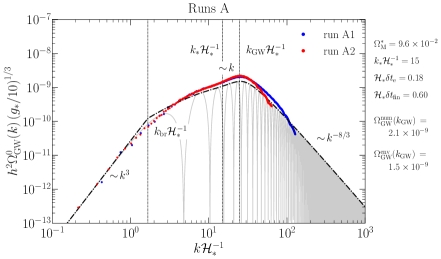
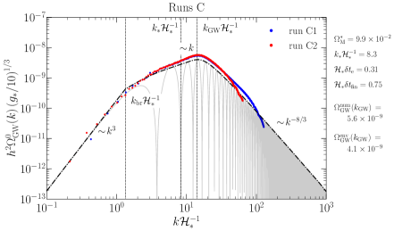
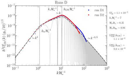
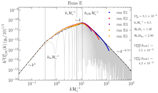
Figure 1: Simulated GW spectra $h^{2}\Omega_{\rm GW}^{0}(k)$ of runs A–E (dots) compared to the analytical model developed in Sec. II.4 assuming constant magnetic stresses: Eq. (18) at $t_{\rm fin}$ (thin gray lines) and its envelope Eq. (28) (dot-dashed black lines). The maximal values over one oscillation of the numerical outputs at each wave number are shown in different colors for runs with different domain sizes, and are combined to show the GW spectra from subhorizon scales up to the scales where the inertial range is developed. Runs A1–E1 (blue dots) are computing the smallest scales resolved, up to a Nyquist wave number of $k_{\rm Ny}{\cal H}_{*}^{-1}=126$. The spectra are shown in terms of $k{\cal H}_{*}^{-1}$ and compensated by $(g_{*}/10)^{-{1\over 3}}$, such that they can be scaled to the specific value of the comoving Hubble rate at the time of generation ${\cal H}_{*}$ and to different values of $g_{*}$.

The GW spectra resulting from the simulations are shown in Fig. 1, together with the analytical solution obtained at $t_{\rm fin}$ [cf. Eq. (18)] and its envelope [cf. Eq. (28)]. As observed in previous simulations (see, e.g., Refs. Roper Pol et al. (2020b, 2022)) and explained in Sec. II.4, we confirm that the $k$ modes of the GW spectra initially grow in time as $\delta t^{2}$ and, after a time $\delta t\sim 1/k$, they start to oscillate around a stationary value. To plot the GW spectra in Fig. 1, we choose the maximal amplitude of such oscillations for each wave number, since we are interested in the envelope of the oscillations. In previous simulations, the low wave number regime was not captured, due to the size of the domains Roper Pol et al. (2020b, 2022); Brandenburg et al. (2021a). Here, we have increased the size of the domain and we have run the simulations for long times (see Table 1, where $t_{\rm end}$ denotes the end of the simulations), such that even the smallest wave numbers of the box reach the oscillatory regime. Since $t_{\rm end}\gg\delta t_{\rm fin}\gtrsim\delta t_{\rm e}$, in the GW spectra of Fig. 1, we observe both the causal $k^{3}$ slope, expected at $k<k_{\rm br}\equiv 1/\delta t_{\rm fin}$, following the model of constant magnetic stresses presented in Sec. II.4.1, and the transition toward the regime that is linear in $k$, expected at $\max({\cal H}_{*},1/\delta t_{\rm fin})<k\lesssim k_{\rm GW}$. The latter was also observed in previous numerical simulations Roper Pol et al. (2020b); Kahniashvili et al. (2021); Roper Pol et al. (2022); Brandenburg et al. (2021c, a).

In order to investigate the spectrum at the smallest wave numbers, we have performed several runs with the same parameters $k_{*}$ and $\Omega_{\rm M}^{*}$, but with different sizes of the cubic domain: respectively, runs A1 and A2, C1 and C2, D1 and D2, and runs E1–E5. Runs A1, B1, C1, and D1 have a resolution of $768^{3}$ mesh points and a size ${\cal H}_{*}L=6\pi$, which corresponds to $k_{0}{\cal H}_{*}^{-1}=1/3$ and a Nyquist wave number of $k_{\rm Ny}{\cal H}_{*}^{-1}=126$. For runs A, C, and D, we have performed a second set of runs, with the same initial conditions but domains doubling the size of A1, C1, and D1, so that the smallest wave number is $k_{0}{\cal H}_{*}^{-1}=1/6$. We reconstruct the final GW spectrum by combining the results of the multiple simulations. This allows us to compute more discretized modes of the GW spectra in different wave number ranges. From Fig. 1, one appreciates that we can accurately reproduce the break from $k^{3}$ to $k^{1}$.

Runs E have the largest eddy turnover time; hence, the $k^{3}$ regime is expected to occur at smaller wave numbers. We have then performed four additional runs, with the largest domain (E5) being 15 times larger than the initial one (E1), corresponding to $k_{0}{\cal H}_{*}^{-1}=1/30$. Runs E have ${\cal H}_{*}\delta t_{\rm fin}>1$: the transition from the $k^{3}$ to the $k^{1}$ regimes should therefore be smoother, according to the constant stress model, and develop a logarithmic dependence in the region $1/\delta t_{\rm fin}<k<{\cal H}_{*}$. Indeed, the GW spectrum follows the curve predicted by the analytical model, i.e., $k^{3}\ln^{2}(1+{\cal H}_{*}/k)$, and the transition of this curve toward the $k^{3}$ regime occurs around the wave number $k_{\rm br}{\cal H}_{*}^{-1}=({\cal H}_{*}\delta t_{\rm fin})^{-1}\simeq 0.3$.

II.6 Fit of the analytical to the numerical GW spectra

Figure 1 shows that the analytical model based on the assumption of constant anisotropic stresses over the time interval $\delta t_{\rm fin}$ accounts for most of the SGWB spectral features: the slopes [including the $k^{3}\ln^{2}(1+{\cal H}_{*}/k)$ increase characteristic of the constant source], the positions at which the slopes change, and the total amplitude. In addition, it predicts accurately the early time evolution of the spectra, starting with an initial phase of growth, proportional to $\delta t^{2}$ and a subsequent oscillatory period, settling in after a time $\delta t\sim 1/k$. However, the analytical model does not provide a value for $\delta t_{\rm fin}$, which is related to the validity of the constant-in-time magnetic stress approximation, and, hence, on the dynamical decay of the turbulent magnetic field, characterized by the eddy turnover time $\delta t_{\rm e}$. Additionally, the numerical spectra have a smoother transition from $k^{3}$ toward the $k^{3}\ln^{2}(1+{\cal H}_{*}/k)$ curve than the piecewise envelope given in Eq. (28), leading to larger values of the numerical GW amplitudes at the peak $k_{\rm GW}$. This is likely due to the fact that the source decays smoothly in time, instead of shutting down abruptly as we assume in the constant model.

Since the MHD turbulent decay occurs on a typical timescale of the order of the eddy turnover time, we expect the source duration parameter $\delta t_{\rm fin}$ to be related to $\delta t_{\rm e}$. The specific values of $\delta t_{\rm fin}$ used in the envelopes shown in Fig. 1 (see Table 1) have been extracted by fitting the analytical solution to the numerical spectra output from each simulation in the $k^{3}$ range. In Fig. 2 (upper panel), we show $\delta t_{\rm fin}$ inferred from the simulations vs $\delta t_{\rm e}$ and fit the linear relation

$$\delta t_{\rm fin}=0.184{\cal H}_{*}^{-1}+1.937\,\delta t_{\rm e}.$$ (40)

Note that, in the limit $\delta t_{\rm e}\rightarrow 0$, this fit yields a finite $\delta t_{\rm fin}$, which is unphysical. Furthermore, we only have one simulated point in the region of large $\delta t_{\rm e}$. Equation (40) is therefore a tentative fit and should not be extrapolated outside the range of $\delta t_{\rm e}$ validated by the simulations.

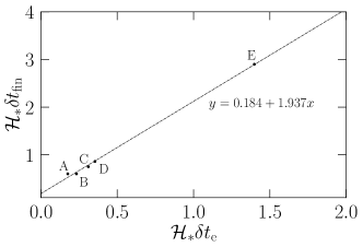
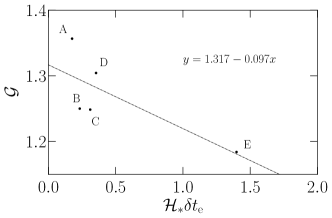
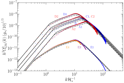
Figure 2: Upper Panel: the points represent the eddy turnover times of the simulations $\delta t_{\rm e}$ and the corresponding values of $\delta t_{\rm fin}$ obtained by fitting the break into $k^{3}$ (occurring at $1/\delta t_{\rm fin}$ according to the analytical model). The dashed line represents the fit of Eq. (40). Middle panel: the points represent the ratio ${\cal G}$ between the numerical and the analytical SGWB amplitudes at the peak. The dashed line represents the fit of Eq. (41). Bottom panel: the SGWBs computed with the analytical model given in Eq. (28) (dot-dashed lines), and from the adjusted model given in Eq. (44) (solid lines), are compared to the results of the MHD simulations (colored points). The compensated model uses the empirical fits shown in the upper and middle panels.

The discrepancy between the amplitude of the numerical and analytical GW spectra at the peak (see Table 1) is expected to decrease as the eddy turnover time increases, since the decay is slower and the assumption of a constant source is appropriate for a larger range of wave numbers. In the middle panel of Fig. 2, we show the ratio between $\Omega_{\rm GW}^{\rm num}(k_{\rm GW})$ and $\Omega_{\rm GW}^{\rm env}(k_{\rm GW})$ [cf. Eq. (29)], which is decreasing, as expected, together with the following fit:

$${\cal G}=\frac{\Omega_{\rm GW}^{\rm num}(k_{\rm GW})}{\Omega_{\rm GW}^{\rm env}(k_{\rm GW})}=1.317-0.097\,{\cal H}_{*}\delta t_{\rm e}.$$ (41)

Altogether, the SGWB spectrum for given initial parameters $k_{*}$ and $\Omega_{\rm M}^{*}$ can be obtained from the analytical model relying on constant stresses developed in Sec. II.4.1 and, in particular, from Eq. (28), fixing $\delta t_{\rm fin}$ via the empirical linear fit of Eq. (40), with the caveat, however, that this relation has only been validated in the range tested with the simulations.

Additionally, one can compensate the second branch of the envelope in Eq. (28), i.e., the regime $1/\delta t_{\rm fin}<k\lesssim k_{\rm GW}$ proportional to $\ln^{2}[1+({\cal H}_{*}/k)]$, by the factor ${\cal G}$ given by the empirical fit of Eq. (41). This compensated model of the envelope of the GW spectrum at $t_{\rm fin}$ reads

$$\Omega_{\rm GW} (k,t_{\rm fin})=\,3\,\biggl{(}\frac{k}{k_{*}}\biggr{)}^{3}\,{\Omega_{\rm M}^{*}}^{2}\frac{{\cal C}(\alpha)}{{\cal A}^{2}(\alpha)}\,\,p_{\Pi}\biggl{(}\frac{k}{k_{*}}\biggr{)}$$

$$\times \left\{\begin{array}[]{ll}\ln^{2}[1+{\cal H}_{*}\delta t_{\rm fin}]&\text{ if }k<k_{\rm br}^{\rm comp},\\ {\cal G}\ln^{2}[1+(k/{\cal H}_{*})^{-1}]&\text{ if }k\geq k_{\rm br}^{\rm comp},\end{array}\right.$$ (44)

where the specific position of the compensated break $k_{\rm br}^{\rm comp}$ is moved from $1/\delta t_{\rm fin}$ to

$$k_{\rm br}^{\rm comp}\,{\cal H}_{*}^{-1}=\Bigl{[}(1+{\cal H}_{*}\delta t_{\rm fin})^{1/\sqrt{\cal G}}-1\Bigr{]}^{-1},$$ (45)

to ensure continuity in the envelope function after compensating one of the branches by ${\cal G}$. The envelopes of the GW spectra are shown in Fig. 2 (bottom panel), both with and without compensating by ${\cal G}$, together with the output of the simulations listed in Table 1.

Whether to use the compensated model Eq. (44) or directly Eq. (28) depends on the particular situation. It can be appreciated from Fig. 2 that the uncompensated model fits the numerical simulations better in the region below the spectral peak ($k<k_{\rm GW}$), but it underpredicts the amplitude at the peak; while the compensated one fits the peak but overpredicts the spectra at smaller wave numbers. Hence, the choice between one or the other model depends on which range of wave numbers one prioritizes to reproduce with the highest accuracy.

III Comparison with PTA results

In this section, we adopt the analytical model developed in Sec. II.4 and validated in Sec. II.5 with MHD simulations and compare the resulting SGWB with the observations reported by the PTA collaborations Arzoumanian et al. (2020); Goncharov et al. (2021); Chen et al. (2021); Antoniadis et al. (2022), thereby inferring the range of parameters $T_{*}$, $k_{\ast}$, and $\Omega_{\rm M}^{*}$, which could account for the PTA results. We remind that we consider a nonhelical magnetic field and assume that the GW production starts once the magnetic field has a fully developed turbulent spectrum.

III.1 PTA results

The three PTA collaborations NANOGrav, PPTA, and EPTA, and the IPTA Collaboration, have independently constrained the amplitude $A_{\rm CP}$ of a red common process (CP) to several pulsars by fitting the power spectral density $S(f)$ to a single power law (PL) of slope $-\gamma$, as Arzoumanian et al. (2020); Goncharov et al. (2021); Chen et al. (2021); Antoniadis et al. (2022)

$$S(f)=\frac{A_{\rm CP}^{2}}{12\pi^{2}}\left(\frac{f}{f_{\rm yr}}\right)^{-\gamma}f_{\rm yr}^{-3},$$ (46)

or to a broken PL as

$$S(f)= \,\frac{A_{\rm CP}^{2}}{12\pi^{2}}\left(\frac{f}{f_{\rm yr}}\right)^{-\gamma}$$

$$\times \,\left[1+\left(\frac{f}{f_{\rm bend}}\right)^{1\over\kappa}\right]^{\kappa\gamma}f_{\rm yr}^{-3},$$ (47)

with $f_{\rm bend}=1.035\times 10^{-8}$ Hz and $\kappa=0.1$. The reference frequency corresponds to 1 yr, $f_{\rm yr}\simeq 3.17\times 10^{-8}{\rm\,Hz}$.

The CP reported by NANOGrav, PPTA, EPTA, and IPTA, characterized by the amplitude $A_{\rm CP}$ and the slope $\gamma$, does not show enough statistical significance toward a quadrupolar correlation over pulsars, following the Hellings-Downs curve, to be ascribed to a SGWB Hellings and Downs (1983); Arzoumanian et al. (2020); Goncharov et al. (2021); Chen et al. (2021); Antoniadis et al. (2022). Interpreting the CP as an actual GW signal, the characteristic strain $h_{\rm c}(f)$ of the corresponding single-PL SGWB would be

$$h_{\rm c}(f)=\sqrt{12\pi^{2}S(f)f^{3}}=A_{\rm CP}\left(\frac{f}{f_{\rm yr}}\right)^{{3-\gamma\over 2}},$$ (48)

and the SGWB spectrum $\Omega_{\rm GW}^{0}(f)$, defined in Eqs. (15) and (31), would be

$$\Omega_{\rm GW}^{0}(f)=\Omega_{\rm yr}\left(\frac{f}{f_{\rm yr}}\right)^{\beta},$$ (49)

with

$$\Omega_{\rm yr}=\frac{2\pi^{2}}{3H_{0}^{2}}f_{\rm yr}^{2}A_{\rm CP}^{2},\quad\beta=5-\gamma.$$ (50)

Analogously, the GW spectrum for the broken PL would be

$$\Omega_{\rm GW}^{0}(f)= \,\Omega_{\rm yr}\left(\frac{f}{f_{\rm yr}}\right)^{\beta}$$

$$\times \,\left[1+\left(\frac{f}{f_{\rm bend}}\right)^{1\over\kappa}\right]^{\kappa(5-\beta)}.$$ (51)

In Fig. 3 (upper panel), we reproduce the 1$\sigma$ and 2$\sigma$ contours of the amplitude $\Omega_{\rm yr}$ as a function of slope $\beta$ reported by NANOGrav using both the single- and broken-PL fits Arzoumanian et al. (2020), and by PPTA Goncharov et al. (2021), EPTA Chen et al. (2021), and IPTA Antoniadis et al. (2022) using the single-PL fit.

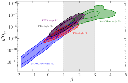
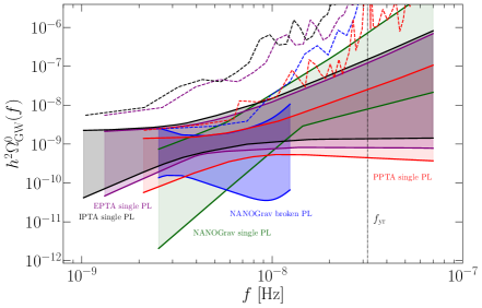
Figure 3: Upper panel: 1$\sigma$ and 2$\sigma$ contours of the amplitude $h^{2}\Omega_{\rm yr}$ vs slope $\beta$ [cf. Eqs. (49) and (51)] derived from the NANOGrav dataset for both the broken-PL (blue) and single-PL (green) fits and from the PPTA (red), EPTA (purple), and IPTA (black) datasets for the single-PL fit Arzoumanian et al. (2020); Goncharov et al. (2021); Chen et al. (2021); Antoniadis et al. (2022). The gray shaded area shows the slopes $\beta\in(1,3)$ characteristic of the SGWB produced by primordial MHD turbulence below the spectral peak; cf. Sec. II.4.1. Lower panel: shaded regions: range of the SGWB spectra $h^{2}\Omega_{\rm GW}^{0}(f)$ of Eqs. (49) and (51), corresponding to the 2$\sigma$ contours given in the upper panel. The vertical line shows the reference frequency $f_{\rm yr}$. Dashed lines: $2\sigma$ maximum amplitude at each frequency—such that larger amplitudes are, in principle, excluded by the PTA observations.

The PTA collaborations present their data in terms of Fourier components of the timing spectrum of the CP. The frequency of the first Fourier mode corresponds to the inverse total observation time, respectively 12.5, 15, 24, and 31 yr for NANOGrav, PPTA, EPTA, and IPTA. From this frequency, up to $f\simeq 1.25\times 10^{-8}{\rm\,Hz}$, the NANOGrav, PPTA, EPTA, and IPTA analyses include, respectively, the first five, six, eight, and ten Fourier modes. At higher frequencies, the Fourier modes have bigger uncertainty and the presence of a PL behavior is less clear Arzoumanian et al. (2020); Goncharov et al. (2021); Chen et al. (2021); Antoniadis et al. (2022). As can be appreciated in Fig. 3, the posterior SGWB amplitude and slope of the NANOGrav dataset differ, depending on whether one fits a single PL to the whole dataset or a broken PL turning to flat noise ($\beta=5$) at high frequencies $f\gtrsim f_{\rm bend}$. This behavior is not observed in the PPTA, EPTA, and IPTA analyses. We therefore consider both the single and broken PL for the NANOGrav result, while we only keep the single PL for PPTA, EPTA, and IPTA.

The part of the MHD-produced SGWB spectrum compatible with the PTA constraints on the spectral slope is the subinertial range below the spectral peak, where $\beta\in(1,3)$ according to Eq. (28) and the numerical results (cf. Fig. 1). The inertial range slope $\beta=-8/3$ corresponds to $\gamma=23/3$, which is too steep compared to the slopes reported by the PTA collaborations (cf. Fig. 3). The peak wave number, separating the subinertial and inertial parts of the spectrum, must satisfy $k_{\rm GW}>k_{*}\geq 2\pi{\cal H}_{*}$ by causality. Using the relation

$$f_{\rm GW}\simeq \,\,1.12\times 10^{-8}$$

$$\times \,\frac{k_{\rm GW}}{2\pi{\cal H}_{*}}\,\frac{T_{*}}{100{\rm\,MeV}}\,\biggl{(}{g_{*}\over 10}\biggr{)}^{1\over 6}\,{\rm\,Hz}\,,$$ (52)

and the value of the GW peak position $k_{\rm GW}\simeq 1.6\,k_{\ast}$, derived in Sec. II.4.1, this translates into frequencies today $f_{\rm GW}\gtrsim 1.8\times 10^{-8}{\rm\,Hz}$, for temperatures around the QCD scale. The subinertial range is therefore expected to cover the region of highest quality PTA data (extending up to $f\simeq 1.25\times 10^{-8}{\rm\,Hz}$), supporting the hypothesis that the latter are compatible with the GW signal from MHD turbulence present at the QCD scale. At lower temperatures $T_{*}\lesssim 70{\rm\,MeV}$, however, $f_{\rm GW}$ decreases below $f\simeq 1.25\times 10^{-8}{\rm\,Hz}$. Moreover, at $T_{*}\lesssim 5{\rm\,MeV}$, the subinertial range exits completely the frequency range of the IPTA dataset if $k_{\ast}=2\pi{\cal H}_{*}$ (IPTA represents the lowest frequencies probed by PTA—cf. Fig. 3).

For the range of initial parameters $k_{*}$ and $\Omega_{\rm M}^{*}$ that fit the PTA observations, the break of the spectrum from the $f^{3}$ to the $f^{1}$ slope occurs in the PTA frequency band; in particular, one can roughly estimate that $10^{-9}{\rm\,Hz}\lesssim f_{\rm br}\lesssim 4\cdot 10^{-9}{\rm\,Hz}$ for temperatures of the order of $100$ MeV. The lowest bound in the above equation is obtained from the values of the magnetic field parameters that maximize the source duration, since $k_{\rm br,min}=1/\delta t_{\rm fin,max}$. Following relation (40), and given $\delta t_{\rm e}=\Bigl{(}k_{*}\sqrt{{3\over 2}\Omega_{\rm M}^{*}}\,\Bigr{)}^{-1}$, one needs to insert the minimal values of both $k_{*}$ and $\Omega_{\rm M}^{*}$. The former corresponds to the horizon scale $k_{*}=2\pi\,{\cal H}_{*}$, while the latter can be roughly estimated imposing that the SGWB peak given in Eq. (29), and evolved till today with Eq. (31), is in the middle of the allowed region, say $\Omega_{\rm GW}^{0}\gtrsim 5\cdot 10^{-10}$ (cf. Fig. 3). This leads to $\Omega_{\rm M}^{*}\gtrsim 0.03$. From the two conditions together, one then finds ${\cal H}_{*}\delta t_{\rm fin,max}\simeq 1.6$, i.e., $k_{\rm br,min}{\cal H}_{*}^{-1}\simeq 0.6$, which gets translated into frequency today via Eq. (52). Conversely, the upper bound of $f_{\rm br}$ can be estimated from the maximal allowed value $\Omega_{\rm M}^{*}=0.1$ and the maximal $k_{*}$. The latter can again be estimated thanks to Eq. (29) repeating the same argument as above, leading to $k_{*}\lesssim 6\pi\,{\cal H}_{*}$. From these values, one finds then ${\cal H}_{*}\delta t_{\rm fin,min}\simeq 0.4$, i.e., $k_{\rm br,max}{\cal H}_{*}^{-1}\simeq 2.2$.

When better quality data will be available, the presence of the break might become important to constrain the origin of the SGWB; cf. the discussion in Secs. III.2 and IV. Moreover, since the maximal source duration is close to the Hubble time ${\cal H}_{*}\delta t_{\rm fin,max}\simeq 1.6$, we expect the transition to occur rather sharply, i.e., without an extended logarithmic transition typical of long sources.

III.2 Constraints on nonhelical magnetic fields using the PTA results

In this section, we use the $2\sigma$ PTA contours of the amplitude and spectral slope of the CP (cf. Fig. 3) to identify the regions in the parameter space of the primordial magnetic field $(k_{\ast},\Omega_{\rm M}^{*})$ leading to a GW signal compatible with the PTA observations, for fixed $T_{*}$. We limit the magnetic field characteristic wave number to be larger than the horizon $k_{\ast}\geq 2\pi{\cal H}_{*}$ and its maximum amplitude to be below 10%, i.e., $\Omega_{\rm M}^{*}\lesssim 0.1$, according to Refs. Shvartsman (1969); Grasso and Rubinstein (1996); Kahniashvili et al. (2011).

For a fixed $T_{*}$, varying the parameters $(k_{\ast},\Omega_{\rm M}^{*})$, we construct the corresponding SGWBs using the analytical model of Eq. (28) and setting $\delta t_{\rm fin}$ to the empirical fit of Eq. (40), validated by the numerical simulations. Note that we are not compensating by the factor $\mathcal{G}$ as in Eq. (44) [cf. also Eq. (41)], since we are interested in fitting the SGWB spectrum at frequencies below the peak: as demonstrated in Sec. III.1, only the subinertial part of the GW spectrum is expected to be in the frequency region where the PTA data could be compatible with a nonzero signal.

For each SGWB so constructed, we compute its slope at each frequency in a subset of the frequency range of the PTA observations. The subset is defined as follows: for the single-PL fit, we choose a range spanning from the first Fourier mode up to $f\simeq 1.25\times 10^{-8}{\rm\,Hz}$, thereby excluding the highest frequencies at which the PTA results have large uncertainties (cf. Sec. III.1); for the broken-PL fit of NANOGrav, we further restrict the range to the maximal frequency $f\simeq 9\times 10^{-9}{\rm\,Hz}$, excluding the part transitioning to the flat power spectral density with $\beta=5$ (cf. Fig. 3).

To compute the slope of the SGWB given in Eq. (28), we simplify the frequency dependence of $p_{\Pi}$ as

$$p_{\Pi}(f/f_{*})=\left\{\begin{array}[]{ll}(f/2f_{*})^{0}&{\rm for}~{}f\leq 2f_{*}\,,\\ (f/2f_{*})^{-11/3}&{\rm for}~{}f>2f_{*}\,,\end{array}\right.$$ (55)

while, in general, it is computed numerically using Eq. (11). The resulting SGWB slope is

$$\beta=\frac{\partial\ln\Omega_{\rm GW}^{0}(f)}{\partial\ln f}=$$

$$\left\{\begin{array}[]{rl}3&\text{if }f<1/(2\pi\delta t_{\rm fin}),\\ 3-2s(f/{\cal H}_{*})&\text{if }1/(2\pi\delta t_{\rm fin})\leq f<2f_{*},\\ \!\!\!-{\textstyle{2\over 3}}-2s(f/{\cal H}_{*})&\text{if }f\geq 2f_{*},\end{array}\right.$$ (59)

where the function $s$ gives the slope of the logarithmic term appearing in Eq. (28),

$$s(x)= \,-\frac{1}{2}\frac{{\rm d}\ln(\ln^{2}[1+1/(2\pi x)])}{{\rm d}\ln x}$$

$$= \,\Bigl{[}(1+2\pi x)\bigl{|}\ln(1+1/(2\pi x)\bigr{|}\Bigr{]}^{-1},$$ (60)

and takes values between 0 and 1 in the low and high $f$ regimes, respectively, yielding the slopes of the SGWB presented in Sec. II.4.

Via Eqs. (49) and (51), one can calculate the range of SGWB amplitudes allowed at 2$\sigma$ by the PTA observations, for a specific slope and frequency, given as a range of $\Omega_{\rm yr}$ (cf. Fig. 3). For a fixed $T_{*}$, we consider that a point in the parameter space $(k_{\ast},\Omega_{\rm M}^{*})$ is compatible with the results reported by one of the PTA collaborations if it provides a SGWB spectrum with amplitude lying within the PTA 2$\sigma$ bounds corresponding to its slope at, at least, one of the frequencies in the chosen PTA frequency subset. Note that the amplitudes reported by the PTA collaborations assume that the GW signal follows a PL, while we expect the subinertial range of the SGWB produced by MHD turbulence to present a spectral shape characterized by two different regimes: one being a PL proportional to $f^{3}$ and the other one being approximately a PL proportional to $f^{1}$ (cf. Sec. II.4). Hence, our approach is conservative and does not rule out SGWBs that present the break from $f^{3}$ to $f^{1}$ within the PTA range of frequencies, which has not been included in the reported analyses by the PTA collaborations. We also allow, in our analysis, the break from $f^{1}$ to $f^{-8/3}$ to occur within the PTA range. The additional consequences of a broken-PL SGWB in cosmology, consistent with NANOGrav observations, have been studied in Ref. Benetti et al. (2022).

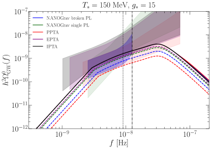
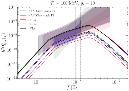
Figure 4: For $T_{*}=150{\rm\,MeV}$ and $g_{*}=15$ in the upper panel, and $T_{*}=100{\rm\,MeV}$ and $g_{*}=10$ in the lower panel, we show the upper boundary (solid lines) and the lower boundary (dashed lines) of the regions compatible with the PTA data at $2\sigma$. To be compatible with NANOGrav with broken PL, each SGWB spectrum must lie in the region within the blue solid and dashed lines; with NANOGrav with single PL, within the green solid and dashed lines; with PPTA, within the red solid and dashed lines; with EPTA, within the purple solid and dashed lines; with IPTA, within the black solid and dashed lines. The shaded areas correspond to the range of allowed values $h^{2}\Omega_{\rm GW}^{0}(f)$ of Eqs. (49) and (51), restricted to the range of slopes of interest for a MHD-produced SGWB, i.e., $\beta\in(1,3)$. The magnetic field characteristic scale is bound to $k_{*}\geq 2\pi{\cal H}_{*}$ and the magnetic energy densities to $\Omega_{\rm M}^{*}\leq 0.1$. The vertical lines show the upper bound of the PTA frequency subset to which we restrain the analysis: $f\simeq 1.25\times 10^{-8}{\rm\,Hz}$ for the single-PL cases (dot-dashed line) and $f\simeq 9\times 10^{-9}{\rm\,Hz}$ for the NANOGrav broken-PL case (dashed line).

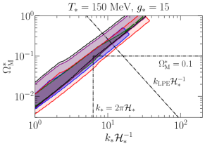
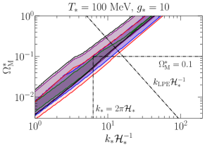
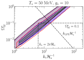
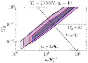
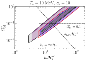
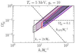
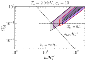
Figure 5: For different values of $T_{*}\in(2,200){\rm\,MeV}$, we show the allowed regions in the $(k_{\ast},\Omega_{\rm M}^{*})$ parameter space, derived as described in the main text from the 2$\sigma$ results of NANOGrav using the broken-PL (blue) and single-PL (green) fits and from the 2$\sigma$ results of EPTA (purple), PPTA (red), and IPTA (black) using the single-PL fits. The vertical and horizontal dot-dashed lines show the physical limits $k_{\ast}\geq 2\pi{\cal H}_{*}$ and $\Omega_{\rm M}^{*}\leq 0.1$, respectively: the allowed parameter region lies within the rectangle. The wave number of the largest processed eddies $\left.k_{*}\right|_{\rm LPE}$ is also shown (dot-dashed diagonal line).

In Fig. 4, we show the curves delimiting the allowed regions in which any SGWB compatible with the PTA observations must lie, obtained using the values of $(k_{\ast},\Omega_{\rm M}^{*})$ derived as described above. To be compatible with the results of a given PTA collaboration, each MHD-produced SGWB must lie within the region delimited by the dashed and solid lines corresponding to that collaboration (i.e., purple lines for EPTA, red for PPTA, and so on). We display the results for energy scales close to the QCD phase transition, e.g., $T_{*}=150{\rm\,MeV}$ and $g_{*}=15$ in the upper panel and $T_{*}=100{\rm\,MeV}$ and $g_{*}=10$ in the lower panel.

If $T_{*}=150{\rm\,MeV}$, the upper boundary of the allowed region is the same for all PTA data; hence, the solid lines superimpose. This roughly corresponds to the point in parameter space $(k_{\ast}=2\pi{\cal H}_{*},\Omega_{\rm M}^{*}=0.1$) (though these values can vary slightly with frequency). The lower boundary of the allowed region is instead different for each dataset considered: NANOGrav with both single and broken PLs, PPTA, EPTA, and IPTA. If $T_{*}=100{\rm\,MeV}$, the region allowed by the NANOGrav single-PL fit corresponds to $\Omega_{\rm M}^{*}$ slightly smaller than 0.1 and $k_{\ast}$ slightly larger than the horizon scale. Note that, in general, the NANOGrav single-PL case is more constraining in terms of $(k_{\ast},\Omega_{\rm M}^{*})$ values, since the minimum slope allowed at 2$\sigma$ is $\beta=1.25$ (cf. Fig. 3), while the other cases allow slopes down to $\beta=1$.

The range of parameters $(k_{\ast},\Omega_{\rm M}^{*})$ compatible with the data of the PTA collaborations at $2\sigma$ are shown in Fig. 5 for temperature scales ranging from 2 to 200 MeV. At temperatures below $1{\rm\,MeV}$, the PTA results cannot be accounted for by a GW signal produced by MHD turbulence, in the limit $\Omega_{\rm M}^{*}\leq 0.1$. For $100{\rm\,MeV}\leq T_{*}\leq 200{\rm\,MeV}$, the magnetic field parameters are strongly constrained: its characteristic wave number $k_{*}$ must be close to the horizon, and its amplitude must be close to the upper bound $\Omega_{\rm M}^{*}\leq 0.1$. Smaller characteristic scales and amplitudes are allowed as $T_{*}$ decreases. For temperatures below $20{\rm\,MeV}$, the point in parameter space $(k_{\ast}=2\pi{\cal H}_{*},\Omega_{\rm M}^{*}=0.1$) is no longer compatible with the data, which prefer magnetic fields with smaller characteristic scales but higher amplitudes, until the latter exceed again their upper bound for temperatures smaller than 1 MeV.

In particular, setting the largest processed eddies as the characteristic scale of the magnetic field, $\left.l_{*}\right|_{\rm LPE}{\cal H}_{*}=\sqrt{{\textstyle{3\over 2}}\Omega_{\rm M}^{*}}$, the resulting SGWB is only compatible with the PTA observations at low temperatures $T_{*}\in(2,50){\rm\,MeV}$ when we limit $\Omega_{\rm M}^{*}\leq 0.1$.

From the allowed parameter regions $(k_{\ast},\Omega_{\rm M}^{*})$ at each $T_{*}$, one can predict at which frequencies the break from $f^{3}$ to $f^{1}$ occurs. While a rough estimate of the break frequency was given in Sec. III.1 for $T_{*}=100{\rm\,MeV}$, we show in Fig. 6 the results of this more refined analysis. It can be appreciated that the smaller the temperature of the phase transition, the smaller the break frequency. Consequently, if this break will be identified in future PTA data, it will help elucidating the SGWB origin: as for the spectral peak $f_{\rm GW}$, we find that $f_{\rm br}$ is connected to the energy scale of the SGWB generating process.

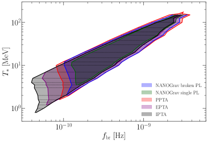
Figure 6: Range of frequencies at which the $f^{3}$ to $f^{1}$ break $f_{\rm br}$ occurs, for the parameters $(k_{\ast},\Omega_{\rm M}^{*})$ compatible with the results of each of the PTA collaborations, for different $T_{*}$ (cf. Fig. 5), in the limit $\Omega_{\rm M}^{*}\leq 0.1$. The horizontal dot-dashed lines correspond to the computed values of $T_{*}$.

III.3 Constraints on the magnetic field amplitude and characteristic scale today

The analysis performed in Sec. III.2 allowed us to constrain the magnetic field amplitude $\Omega_{\rm M}^{*}$ and characteristic scale $k_{\ast}$ at several fixed temperature values $T_{*}$. In this section, we derive the constraints on the comoving magnetic field strength $B_{*}$ and characteristic length $l_{*}$ compatible with the PTA results. We then compare them with other constraints on primordial magnetic fields, in particular at recombination. The results are shown in Fig. 7.

To begin with, we transform the constraints on $\Omega_{\rm M}^{*}$ to constraints on the comoving magnetic field root mean square amplitude $B_{*}=\sqrt{\langle\mathchoice{\mbox{\boldmath$\displaystyle B$}}{\mbox{\boldmath$\textstyle B$}}{\mbox{\boldmath$\scriptstyle B$}}{\mbox{\boldmath$\scriptscriptstyle B$}}{}^{2}\rangle}$:

$$B_{*} = \sqrt{2\,{\cal E}_{\rm M}^{*}\,\mu_{0}}\,\biggl{(}\frac{a_{*}}{a_{0}}\biggr{)}^{2}$$ (61)

$$\simeq 3.87\,\sqrt{{\Omega_{\rm M}^{*}}}\,\biggl{(}\frac{g_{*}}{10}\biggr{)}^{-{1\over 6}}\mu{\rm G},$$

where ${\cal E}_{\rm M}^{*}=\Omega_{\rm M}^{*}\,{\cal E}_{\rm rad}^{*}$, the factor $({a_{*}}/{a_{0}})^{2}$ accounts for the fact that the magnetic field is comoving, and we have recovered $c=3\times 10^{8}{\rm\,m}/{\rm\,s}=9.72\times 10^{-15}{\rm\,Mpc}/{\rm\,s}$ and $\mu_{0}=40\pi$ G² (J/m³)^-1, otherwise set to $c=\mu_{0}=1$, since in this section we want to express $B_{*}$ in Gauss (G) and $l_{*}$ in parsecs. Consequently, ${\cal E}_{\rm rad}^{*}=\pi^{2}g_{*}T_{*}^{4}/(30(\hbar c)^{3})$ Kolb and Turner (1990). The characteristic comoving length scale $l_{*}$ can be expressed in parsecs using Eq. (37):

$$l_{*}=\frac{2\pi}{k_{\ast}}\simeq 5.4\,\frac{{\cal H}_{*}}{ck_{\ast}}\frac{100{\rm\,MeV}}{T_{*}}\biggl{(}\frac{g_{*}}{10}\biggr{)}^{-{1\over 6}}{\rm pc}.$$ (62)

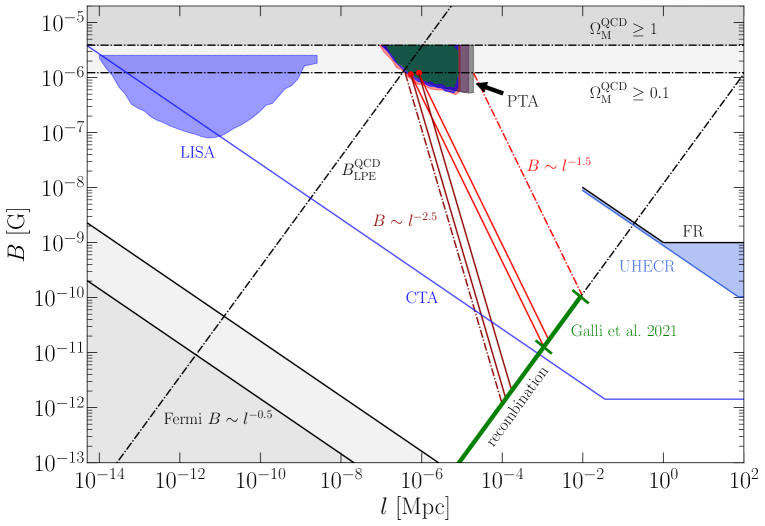
Figure 7: Region in the magnetic field parameter space, given by its comoving amplitude $B$ and characteristic scale $l$, compatible with the observations of the different PTA collaborations: in blue, NANOGrav with broken PL; in green, NANOGrav with single PL; in red, PPTA; in purple, EPTA; in black, IPTA. The parameter space region accessible to LISA is shown in light blue. The horizontal dot-dashed lines show the bounds $\Omega_{\rm M}^{*}\leq 1$, and $\Omega_{\rm M}^{*}\leq 0.1$ from nucleosynthesis Shvartsman (1969); Grasso and Rubinstein (1996); Kahniashvili et al. (2011). The black dot-dashed diagonal lines show i) the magnetic field amplitude when the characteristic scale corresponds to the largest processed eddies at the QCD phase transition $\left.l_{*}\right|_{\rm LPE}$ [cf. Eq. (63)]; ii) the magnetic field amplitude reached at recombination [cf. Eq. (64)]. The dot-dashed red and brown lines show the evolutionary paths of the extremities of the parameter space region compatible with the PTA results up to recombination, following compressible (red) and incompressible (brown) MHD free decay. The solid red and brown lines indicate the evolutionary paths of an initial field with $k_{\ast}=2\pi{\cal H}_{*}$ and $\Omega_{\rm M}^{*}=0.1$ at $T_{*}=100{\rm\,MeV}$ and $g_{*}=10$ (right red dot) and at $T_{*}=150{\rm\,MeV}$ and $g_{*}=15$ (left red dot). The green line indicates the upper limit $B\lesssim 0.1$ nG, and the range $B_{\rm rec}\in(0.013,0.1)$ nG, proposed to alleviate the Hubble tension, both derived in Ref. Galli et al. (2022) from CMB constraints on the baryon clumping. The black solid diagonal lines show the Fermi Large Area Telescope (LAT) lower bound on the intergalactic magnetic field from timing of the blazar signal (darker gray area) and from the search of extended emission (lighter gray area) Ackermann et al. (2018). The blue line shows the expected sensitivity of CTA Korochkin et al. (2021). At larger scales, the upper bound from Faraday rotation (FR) is shown Pshirkov et al. (2016), and the blue shaded region indicates the observations of UHECR from the Perseus-Pisces supercluster Abbasi et al. ; Neronov et al. . Note that the latter constraints refer to present time magnetic field strength and characteristic scale, and they have been cut to avoid intersecting the evolutionary paths from the QCD phase transition up to recombination in the plot, for clarity.

The region of $B_{*}$ and $l_{*}$ values allowed by the PTA results is shown in Fig. 7, and it is limited by $T_{*}\in(1,200){\rm\,MeV}$, $l_{*}\in(0.4,20)$ pc, and $B_{*}\in(0.5,1.2)\,\mu$G, when we consider the nucleosynthesis constraint $\Omega_{\rm M}^{*}\leq 0.1$, which gives $B_{*}\leq 1.2\,\mu$G $(g_{*}/10)^{-{1\over 6}}$. If we allow $0.1\leq\Omega_{\rm M}^{*}\leq 1$, then the region extends to $B_{*}\in(0.5,3.8)\,\mu$G, $l_{*}\in(0.1,20){\rm\,pc}$, and $T_{*}\in(0.2,350){\rm\,MeV}$.

Figure 7 also shows the region in parameter space $(B_{*},\,l_{*})$ that could be probed by the Laser Interferometer Space Antenna (LISA). We have obtained it via a similar analysis to that of Sec. III.2, using the model developed in Sec. II.4.1, and considering the PL sensitivity of LISA for a threshold signal-to-noise ratio of 10 and 4 yr of mission duration Caprini et al. (2019); Schmitz (2021). LISA could probe the SGWB from primordial magnetic fields with amplitudes in the range $B_{*}\in(0.08,0.8)\,\mu$G and characteristic scales in the range $l_{*}\in(2.6\times 10^{-8},\,8\times 10^{-4})$ pc, with a range of temperatures $T_{*}\in(50{\rm\,GeV},2000{\rm\,TeV})$ when $\Omega_{\rm M}^{*}\leq 0.1$. If we allow $0.1\leq\Omega_{\rm M}^{*}\leq 1$, then the range of temperatures compatible with LISA extends to $T_{*}\in(5{\rm\,GeV},5000{\rm\,TeV})$ and the primordial magnetic field parameters to $l_{*}\in(10^{-8},2.6\times 10^{-3})\,{\rm\,pc}$ and $B_{*}\in(0.08,2.5)\,\mu$G.

Along with the GW production, the primordial magnetic field evolves following the MHD turbulent free decay. For nonhelical fields, the direct cascade leads to the scaling $B\propto l^{-5/2}$ for incompressible turbulence and $B\propto l^{-3/2}$ for compressible turbulence Durrer and Neronov (2013); Banerjee and Jedamzik (2004). Furthermore, the turbulent evolution is expected to drive the magnetic characteristic scale to the one of the largest processed eddies Banerjee and Jedamzik (2004), $\left.l_{*}\right|_{\rm LPE}{\cal H}_{*}=\sqrt{{3\over 2}\Omega_{\rm M}^{*}}$. The magnetic field amplitude at this scale can be obtained combining Eqs. (61) and (62):

$$\left.B_{*}\right|_{\rm LPE}\simeq 3.6\,\frac{\left.l_{*}\right|_{\rm LPE}}{1{\rm\,pc}}\,\frac{T_{*}}{100{\rm\,MeV}}\,\mu{\rm G}.$$ (63)

This equation can be readily applied to find as well the magnetic field amplitude at recombination Banerjee and Jedamzik (2004); Durrer and Neronov (2013)

$$\left.B_{\rm rec}\right|_{\rm LPE}\simeq 10^{-2}\,{\rm nG}\,\frac{\left.l_{\rm rec}\right|_{\rm LPE}}{1{\rm\,kpc}},$$ (64)

where we have used $T_{\rm rec}=0.32$ eV Durrer (2008). Both Eqs. (63) and (64) are shown in Fig. 7 by black dot-dashed lines.

The evolutionary paths, from the QCD phase transition up to the epoch of recombination, of the extremities of the $(B_{*},\,l_{*})$ region compatible with the PTA observations are shown by red (compressible) and brown (incompressible) dot-dashed lines in Fig. 7. In particular, the solid lines indicate the evolutionary paths of a primordial magnetic field with $k_{\ast}=2\pi{\cal H}_{*}$ and $\Omega_{\rm M}^{*}=0.1$ at $T_{*}=150{\rm\,MeV}$ and $g_{*}=15$ and at $T_{*}=100{\rm\,MeV}$ and $g_{*}=10$.

In Ref. Neronov et al. (2021), it was shown that the magnetic field compatible with the NANOGrav results Arzoumanian et al. (2020) would correspond at recombination to a magnetic field of the same order of magnitude of those analyzed in Refs. Jedamzik and Abel ; Jedamzik and Pogosian (2020). In these works, it was pointed out that a sub-nano-Gauss prerecombination magnetic field would induce additional baryon inhomogeneities, which would enhance the recombination rate, thereby changing the CMB spectrum in a way that would alleviate the Hubble tension. Reference Galli et al. (2022) derived updated constraints on the baryon clumping from data of CMB experiments, of about $b\lesssim 0.5$ at 95% confidence level, which can be translated into an upper limit on the prerecombination magnetic field amplitude $B_{\rm rec}\lesssim 0.1$ nG. In addition, they derive a range $b\in(0.16,\,0.55)$ that is compatible with a value $H_{0}\approx 70{\rm\,km}{\rm\,s}^{-1}{\rm\,Mpc}^{-1}$, relieving the Hubble tension. Such values of the clumping factor correspond to magnetic field strengths $B_{\rm rec}\in(0.013,\,0.1)$ nG, which include phase transition and inflationary produced magnetic fields Jedamzik and Saveliev (2019); Galli et al. (2022). The upper limit and, in particular, the range derived to alleviate the Hubble tension are indicated in Fig. 7 by a green line and interval, respectively.

The end points of the evolutionary paths of the magnetic field amplitude and characteristic scale compatible with the PTA results, representing their values at recombination, lie on the line given in Eq. (64), where we also superimpose the constraint $B_{\rm rec}\lesssim 0.1$ nG from Ref. Galli et al. (2022). It can be appreciated that they are compatible. We therefore confirm that a magnetic field at the QCD scale could both account for the PTA results and alleviate the Hubble tension, as pointed out in Refs. Jedamzik and Pogosian (2020); Galli et al. (2022), depending on the parameters $k_{\ast}$ and $\Omega_{\rm M}^{*}$ of the initial field and whether the developed MHD turbulence of the primordial plasma is compressible or incompressible.

Furthermore, in Fig. 7, we report the lower bounds on the magnetic field amplitude from the Fermi gamma-ray telescope Ackermann et al. (2018); Durrer and Neronov (2013); Neronov and Semikoz (2009); Korochkin et al. (2021). It was shown recently that CTA is sensitive to primordial magnetic fields up to 0.01 nG (cf. Fig. 7) in the voids of the LSS Korochkin et al. (2021). The signal from a primordial magnetic field produced in phase transitions can be distinguished from one produced during inflation since the latter is expected to produce a coherent signal among several nearby blazars Korochkin et al. .

The magnetic field can be additionally constrained from above by observations of ultra-high-energy cosmic rays (UHECR) sources. Recent observations of UHECR from the Perseus-Pisces supercluster Abbasi et al. allowed one for the first time to put an upper limit on the primordial magnetic field in the voids of the LSS Neronov et al. . Finally, the upper bounds from Faraday rotation measurements Pshirkov et al. (2016) are shown in Fig. 7.

III.4 Role of the magnetogenesis scenario on the SGWB spectrum

Primordial magnetic fields can be either produced or amplified during the QCD phase transition (see Refs. Durrer and Neronov (2013); Subramanian (2016); Vachaspati (2021) for reviews and references therein). In particular, some magnetogenesis scenarios at the QCD scale have been proposed; see e.g., Refs. Quashnock et al. (1989); Vachaspati (1991); Cheng and Olinto (1994); Sigl et al. (1997); Forbes and Zhitnitsky ; Tevzadze et al. (2012); Miniati et al. (2018). Previous works performing simulations to compute the SGWB produced by MHD turbulence, both in the general context of phase transitions Roper Pol et al. (2020b); Brandenburg et al. (2021c); Kahniashvili et al. (2021); Roper Pol et al. (2022) and, more specifically, at the QCD phase transition Brandenburg et al. (2021a), have modeled the magnetic field production via a forcing term in the induction equation [cf. Eq. (4)]. These simulations show that, in general, the efficiency of the GW production $q=k_{\ast}{\cal H}_{*}^{-1}\sqrt{h^{2}\,\Omega_{\rm GW}^{0}}/\Omega_{\rm M}^{*}$ is larger when the magnetic field is driven than when it is given at the initial time of the simulation Roper Pol et al. (2020b, 2022). The spectral shape is also affected, mostly in the inertial range, i.e., at frequencies larger than $f_{\rm GW}$, where it presents a steeper forward cascade toward smaller scales Roper Pol et al. (2020b, 2022); Brandenburg et al. (2021a). In the subinertial range, the slope can also be slightly modified, presumably due to deviations from Gaussianity Brandenburg and Boldyrev (2020); Brandenburg et al. (2021c); Roper Pol et al. (2022).

However, since the magnetogenesis dynamics are still uncertain and are model dependent, previous simulations do not necessarily reproduce the actual physical mechanism of magnetic field production that might have operated in the early Universe. In any case, their results suggest that the model presented in our work, which assumes that the magnetic field is already present at the beginning of the simulation, might be underpredicting the SGWB signal (or, equivalently, overestimating the magnetic field strength necessary to explain the PTA data). This can be appreciated in Fig. 8, where we compare the SGWB obtained from the analytical model of Eqs. (28) and (40), with the one obtained in Ref. Brandenburg et al. (2021a) for nonhelical fields with $\Omega_{\rm M}^{*}=0.1$ and $k_{\ast}=10\,{\cal H}_{*}$ at $T_{*}=100{\rm\,MeV}$. We also show, for comparison, the SGWB obtained in Ref. He et al. from an inflationary magnetogenesis scenario with an end-of-reheating temperature around the QCD scale, both for a nonhelical magnetic field with $\Omega_{\rm M}^{*}\simeq 0.04$ and $k_{\ast}\simeq 2.9\,{\cal H}_{*}$ at $T_{*}=150{\rm\,MeV}$ and a helical field with $\Omega_{\rm M}^{*}\simeq 0.1$ and $k_{\ast}\simeq 6.7\,{\cal H}_{*}$ at $T_{*}=120{\rm\,MeV}$.

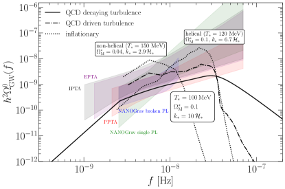
Figure 8: SGWBs generated by different sources operating around the QCD scale compared to the PTA results. The black solid line shows the analytical model developed in Sec. II.4, validated with MHD turbulence simulations in Sec. II.5 (“QCD decaying turbulence”). The dot-dashed line shows the SGWB obtained in Ref. Brandenburg et al. (2021a) by adding a forcing term in the induction equation to model the magnetic field generation (“QCD driven turbulence”). The dotted lines correspond to the inflationary magnetogenesis scenario of Ref. He et al. with an end-of-reheating temperature around the scale of the QCD phase transition (“inflationary”).

IV Comparison with the SGWB from supermassive black hole binaries

The most commonly considered model of the SGWB in the nanohertz frequency range is that of the collective GW signal from mergers of supermassive black hole binaries (SMBHB). This unrelated signal serves as a “foreground” for the cosmological SGWB signal detection. It is interesting to analyze whether the two types of SGWB can be distinguished by current and future detections.

Straightforward analytical estimates Phinney ; Sampson et al. (2015) show that the cumulative spectrum of the GW emission from a population of SMBHB losing energy exclusively via gravitational radiation is expected to follow a PL with the slope $(3-\gamma)/2=-2/3$ or, equivalently, $\beta=2/3$ [cf. Eqs. (48) and (49)]. This naive model is shown by the black dotted line in Fig. 9. The large error bars of the PTA measurements do not allow one to distinguish between this slope and the expected slope of the SGWB produced by primordial MHD turbulence (shown by the blue line in Fig. 9).

This simple analytical model $\Omega_{\rm GW}^{0}(f)\sim f^{2/3}$ does not take into account a number of effects that influence the shape of the SGWB from supermassive black hole mergers. One of these effects is related to the “last parsec” problem Sampson et al. (2015), the fact that the timescale of the gravitational energy loss on GW emission is longer than the Hubble time for binaries with subparsec binary separations. Orbital periods of such binaries are about 10 yr and the GW emission from these systems falls into the frequency range of the PTA results. SMBHB can occur on the time span of the age of the Universe only if there exists a nongravitational energy loss that resolves the last parsec problem. In any case, this alternative energy loss channel removes energy from the GW signal and suppresses the GW spectral power. This results in deviations from the PL scaling $\beta=2/3$.

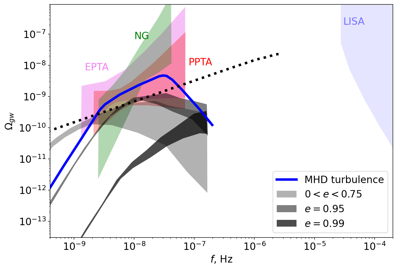
Figure 9: Possible SGWB from supermassive black hole mergers and by MHD turbulence, using the analytical model developed in Sec. II.4, compared to the PTA results. The black dotted line is proportional to $f^{2/3}$.

Dynamical friction produced by scattering of stars may be a viable solution to the last parsec problem if the eccentricity of the binary black hole systems is taken into account. Examples of modeling of this effect Kelley et al. (2017) are shown by gray-shaded bands in Fig. 9. The suppression of the GW power occurs in the frequency range of PTAs for highly eccentric systems, with $e\geq 0.95$.

Still another effect may produce a second break in the spectrum at higher frequency, as seen in Fig. 9. This break occurs due to the discreetness of the spatial distribution of sources contributing to the SGWB Sesana et al. (2008); Kelley et al. (2017).

Overall, the combination of the two breaks may result in a SGWB spectrum from SMBHB similar to that produced from MHD turbulence. This is clear from a comparison of the model spectrum discussed above (blue line in Fig. 9) with the state-of-art models for the supermassive black hole SGWB spectra (gray bands in Fig. 9), calculated based on the cosmological hydrodynamical model Illustris Sijacki et al. (2015).

It still should be possible to distinguish between the SMBHB and cosmological models using the statistics of individual binary system detections at higher frequencies. Even though the diffuse background flux is suppressed at high frequencies because of the discreetness of the source distribution, individual sources (not considered anymore as part of the diffuse flux) become detectable. Their spectra typically extend well into the frequency range of LISA and their cumulative flux still follows the analytical $f^{2/3}$ scaling, with a moderate suppression in the LISA frequency range due to the fact that the GW emission from higher mass systems does not reach LISA sensitivity band. If the supermassive black hole SGWB is at the level of the current PTA measurements, LISA should be able to detect numerous individual merging systems and independently constrain the normalization of the supermassive black hole merger part of the background Sesana et al. (2008).

V Conclusions

In this work, we have analyzed the GW signal produced by the anisotropic stresses of a primordial nonhelical magnetic field. We suppose that some process related to a primordial phase transition—in particular, here we focus on the QCD phase transition—generates the initial magnetic field. Since both the kinetic viscosity and the resistivity are very low in the early Universe, the magnetic field induces MHD turbulence in the primordial plasma. For simplicity, we do not model the magnetic field generation nor the buildup of the turbulent cascade, but we set as initial condition for the GW production a magnetic field with fully developed turbulent spectrum. This is an important caveat of our analysis. We have chosen this approach to better keep under control the physics of the GW production and consequently gain insight on the resulting GW spectral shape, starting from simple initial conditions. The chosen initial conditions are conservative: we expect the MHD turbulent magnetic spectrum to develop for any magnetogenesis mechanism and the amplitude of the SGWB to increase if an initial period of magnetic field generation is included in the analysis. We plan to increase the level of complexity by analyzing concrete magnetic field production mechanisms in future works.

The first important result of our analysis is that the GW signal can be easily reproduced by assuming that the magnetic stresses sourcing the GWs are constant in time over a time interval $\delta t_{\rm fin}$. The reason is that, for most of the spectral modes of the GW signal, the typical time of the GW production is shorter than the typical time of the magnetic field evolution since, by causality, the Alfvén speed is smaller than the speed of light. We provide in Eq. (28) a simple formula for the resulting SGWB spectrum, in which the spectral slopes and the scaling with the source parameters (i.e., energy scale of the source and magnetic field’s amplitude and characteristic scale) are apparent.

This formula can be used in general as a template for the SGWB spectrum from fully developed MHD turbulence. We have in fact validated it with a series of MHD simulations initiated with a fully developed magnetic field spectrum and no initial bulk velocity. These have been performed using the Pencil Code Brandenburg et al. (2021b) and consist in several runs that cover a wide range of modes, from the large super-Hubble scales up to the high wave numbers of the magnetic field inertial range. The GW spectra outputs from the simulations are well reproduced by the template obtained under the assumption of constant anisotropic stress. In particular, they both feature a break at a characteristic wave number corresponding to the inverse duration of the GW source, where the causal $k^{3}$ increase transitions to a linear increase, more or less smoothly depending on whether the source lasts more or less than one Hubble time. We indeed use the break position in the simulations to fix the source duration parameter $\delta t_{\rm fin}$, which is a free parameter of the analytical model, in terms of the eddy turnover time $\delta t_{\rm e}$.

We have then applied our results to the case of the QCD phase transition. As pointed out in a previous work Neronov et al. (2021), the GW signal from MHD turbulence occurring close to the QCD energy scale in the early Universe can account for the CP reported recently by the observations of the PTA collaborations: NANOGrav, PPTA, EPTA, and IPTA. Here we have used the simulation-validated SGWB template Eq. (28) and compared it to the PTA results.

Several points deserve to be highlighted concerning this particular possible explanation of the PTA CP. First of all, the region of the MHD-produced SGWB spectrum that is compatible with the PTA constraints on the CP spectral index is the subinertial region, and for temperature scales of the order of the QCD phase transition, the subinertial region naturally falls in the frequency range where the PTA data present less uncertainty.

Second, the break in the SGWB spectrum is also expected to fall in the same best quality data frequency region, for temperatures around 100 MeV. The position of the break is correlated to the energy scale of the process that generated the magnetic field and, in turn, the SGWB. Therefore, measuring the position of the break in the future PTA data offers the interesting opportunity to pin down its origin, especially if the PTA observations can be combined with LISA to help disentangle this SGWB of primordial origin from the one due to SMBHB.

Third, the energy scale of the magnetogenesis mechanism, and therefore of the GW production, is quite constrained already by the PTA data: it must be in the range $1{\rm\,MeV}<T_{*}<200{\rm\,MeV}$; otherwise, this scenario fails to explain the PTA results in the limit $\Omega_{\rm M}^{*}\leq 0.1$. At the same time, the initial amplitude of the magnetic field must be at least 1% of the radiation energy density, and its characteristic scale must be within 10% of the horizon scale. It is therefore not unreasonable to expect that future PTA data will be able to falsify the hypothesis of the SGWB signal from MHD turbulence.

At last, the ranges of magnetic field amplitudes and characteristic scales that can account for the PTA CP through the GW signal they generate could also affect the evolution of the baryon density fluctuations at recombination, effectively enhancing the recombination process and lowering the sound horizon at recombination Jedamzik and Pogosian (2020); Galli et al. (2022); Jedamzik et al. (2021). The presence of a magnetic field at recombination with present-time strength of about $0.01\lesssim B_{\rm rec}\lesssim 0.1$ nG was recently proposed as a possible way to alleviate the Hubble tension Galli et al. (2022); Jedamzik and Pogosian (2020). Such a field could be detected in the voids of Large Scale Structure with a future CTA gamma-ray observatory Korochkin et al. (2021). We find here that the SGWB which such a magnetic field would produce offers a further observational channel to test this hypothesis.

DATA AVAILABILITY

The source code used for the simulations of this study, the Pencil Code, is freely available Brandenburg et al. (2021b). The simulation datasets are also publicly available Roper Pol et al. . The calculations, the simulation data, and the routines generating the plots are publicly available on GitHub Roper Pol .

ACKNOWLEDGEMENTS

We are grateful to Ruth Durrer and Tina Kahniashvili for their useful feedback and comments. Support through the French National Research Agency (ANR) project MMUniverse (ANR-19-CE31-0020) is gratefully acknowledged. A.R.P. also acknowledges support from the Shota Rustaveli National Science Foundation (SRNSF) of Georgia (Grant No. FR/18-1462). We acknowledge the allocation of computing resources provided by the Grand Équipement National de Calcul Intensif (GENCI) to the project “Opening new windows on Early Universe with multi-messenger astronomy” (A0090412058).

References

- Neronov and Vovk (2010) A. Neronov and I. Vovk, “Evidence for strong extragalactic magnetic fields from fermi observations of tev blazars,” Science 328, 73 (2010).
- Ackermann et al. (2018) M. Ackermann et al. (Fermi-LAT Collaboration), “Search for spatial extension in high-latitude sources detected by the Fermi Large Area Telescope,” Astrophys. J. Suppl. 237, 32 (2018), arXiv:1804.08035 [astro-ph.HE] .
- Durrer and Neronov (2013) R. Durrer and A. Neronov, “Cosmological magnetic fields: Their generation, evolution and observation,” Astron. Astrophys. Rev. 21, 62 (2013), arXiv:1303.7121 [astro-ph.CO] .
- Vachaspati (2021) T. Vachaspati, “Progress on cosmological magnetic fields,” Rep. Prog. Phys. 84, 074901 (2021), arXiv:2010.10525 [astro-ph.CO] .
- Ahonen and Enqvist (1996) J. Ahonen and K. Enqvist, “Electrical conductivity in the early universe,” Phys. Lett. B 382, 40 (1996), arXiv:hep-ph/9602357 .
- Brandenburg et al. (1996) A. Brandenburg, K. Enqvist, and P. Olesen, “Large scale magnetic fields from hydromagnetic turbulence in the very early universe,” Phys. Rev. D 54, 1291 (1996), arXiv:astro-ph/9602031 .
- Caprini and Figueroa (2018) C. Caprini and D. G. Figueroa, “Cosmological backgrounds of gravitational waves,” Classical Quantum Gravity 35, 163001 (2018), arXiv:1801.04268 [astro-ph.CO] .
- Sazhin (1978) M. V. Sazhin, “Opportunities for detecting ultralong gravitational waves,” Soviet Ast. 22, 36 (1978).
- Detweiler (1979) S. L. Detweiler, “Pulsar timing measurements and the search for gravitational waves,” Astrophys. J. 234, 1100 (1979).
- Deryagin et al. (1986) D. V. Deryagin, D. Y. Grigoriev, V. A. Rubakov, and M. V. Sazhin, “Possible anisotropic phases in the early Universe and gravitational wave background,” Mod. Phys. Lett. A 01, 593 (1986).
- Hogan (1986) C. J. Hogan, “Gravitational radiation from cosmological phase transitions,” Mon. Not. R. Astron. Soc. 218, 629 (1986).
- Witten (1984) E. Witten, “Cosmic separation of phases,” Phys. Rev. D 30, 272 (1984).
- Signore and Sanchez (1989) M. Signore and N. G. Sanchez, “Comments on cosmological gravitational waves background and pulsar timings,” Mod. Phys. Lett. A 04, 799 (1989).
- Thorsett and Dewey (1996) S. E. Thorsett and R. J. Dewey, “Pulsar timing limits on very low frequency stochastic gravitational radiation,” Phys. Rev. D 53, 3468 (1996).
- Caprini et al. (2010) C. Caprini, R. Durrer, and X. Siemens, “Detection of gravitational waves from the QCD phase transition with pulsar timing arrays,” Phys. Rev. D 82, 063511 (2010), arXiv:1007.1218 [astro-ph.CO] .
- Arzoumanian et al. (2020) Z. Arzoumanian et al. (NANOGrav Collaboration), “The NANOGrav 12.5 yr data set: Search for an isotropic stochastic gravitational-wave background,” Astrophys. J. Lett. 905, L34 (2020), arXiv:2009.04496 [astro-ph.HE] .
- Goncharov et al. (2021) B. Goncharov et al., “On the evidence for a common-spectrum process in the search for the nanohertz gravitational-wave background with the Parkes Pulsar Timing Array,” Astrophys. J. Lett. 917, L19 (2021), arXiv:2107.12112 [astro-ph.HE] .
- Chen et al. (2021) S. Chen et al., “Common-red-signal analysis with 24-yr high-precision timing of the European Pulsar Timing Array: Inferences in the stochastic gravitational-wave background search,” Mon. Not. R. Astron. Soc. 508, 4970 (2021), arXiv:2110.13184 [astro-ph.HE] .
- Antoniadis et al. (2022) J. Antoniadis et al., “The International Pulsar Timing Array second data release: Search for an isotropic gravitational wave background,” Mon. Not. R. Astron. Soc. 510, 4873 (2022), arXiv:2201.03980 [astro-ph.HE] .
- Hellings and Downs (1983) R. W. Hellings and G. S. Downs, “Upper limits on the isotropic gravitational radiation background from pulsar timing analysis,” Astrophys. J. Lett. 265, L39 (1983).
- Haehnelt (1994) M. G. Haehnelt, “Low-frequency gravitational waves from supermassive black-holes,” Mon. Not. R. Astron. Soc. 269, 199 (1994), arXiv:astro-ph/9405032 [astro-ph] .
- Sesana et al. (2004) A. Sesana, F. Haardt, P. Madau, and M. Volonteri, “Low-frequency gravitational radiation from coalescing massive black hole binaries in hierarchical cosmologies,” Astrophys. J. 611, 623 (2004), arXiv:astro-ph/0401543 .
- Sesana et al. (2008) A. Sesana, A. Vecchio, and C. N. Colacino, “The stochastic gravitational-wave background from massive black hole binary systems: Implications for observations with pulsar timing arrays,” Mon. Not. R. Astron. Soc. 390, 192–209 (2008), arXiv:0804.4476 [astro-ph] .
- Vagnozzi (2021) S. Vagnozzi, “Implications of the NANOGrav results for inflation,” Mon. Not. R. Astron. Soc. 502, L11 (2021), arXiv:2009.13432 [astro-ph.CO] .
- Li et al. (2021a) H.-H. Li, G. Ye, and Y.-S. Piao, “Is the NANOGrav signal a hint of dS decay during inflation?” Phys. Lett. B 816, 136211 (2021a), arXiv:2009.14663 [astro-ph.CO] .
- Kuroyanagi et al. (2021) S. Kuroyanagi, T. Takahashi, and S. Yokoyama, “Blue-tilted inflationary tensor spectrum and reheating in the light of NANOGrav results,” J. Cosmol. Astropart. Phys. 01, 071 (2021), arXiv:2011.03323 [astro-ph.CO] .
- Sharma (2022) R. Sharma, “Constraining models of inflationary magnetogenesis with NANOGrav data,” Phys. Rev. D 105, L041302 (2022), arXiv:2102.09358 [astro-ph.CO] .
- Lazarides et al. (2021) G. Lazarides, R. Maji, and Q. Shafi, “Cosmic strings, inflation, and gravity waves,” Phys. Rev. D 104, 095004 (2021), arXiv:2104.02016 [hep-ph] .
- (29) Z. Yi and Z.-H. Zhu, “NANOGrav signal and LIGO-Virgo primordial black holes from Higgs inflation,” arXiv:2105.01943 [gr-qc] .
- (30) Y. He, A. Roper Pol, and A. Brandenburg, “Leading-order nonlinear gravitational waves from reheating magnetogeneses,” arXiv:2110.14456 [astro-ph.CO] .
- Ellis and Lewicki (2021) J. Ellis and M. Lewicki, “Cosmic string interpretation of NANOGrav pulsar timing data,” Phys. Rev. Lett. 126, 041304 (2021), arXiv:2009.06555 [astro-ph.CO] .
- Blasi et al. (2021) S. Blasi, V. Brdar, and K. Schmitz, “Has NANOGrav found first evidence for cosmic strings?” Phys. Rev. Lett. 126, 041305 (2021), arXiv:2009.06607 [astro-ph.CO] .
- Buchmuller et al. (2020) W. Buchmuller, V. Domcke, and K. Schmitz, “From NANOGrav to LIGO with metastable cosmic strings,” Phys. Lett. B 811, 135914 (2020), arXiv:2009.10649 [astro-ph.CO] .
- Samanta and Datta (2021) R. Samanta and S. Datta, “Gravitational wave complementarity and impact of NANOGrav data on gravitational leptogenesis,” J. High Energy Phys. 05, 211 (2021), arXiv:2009.13452 [hep-ph] .
- Bian et al. (2021) L. Bian, R.-G. Cai, J. Liu, X.-Y. Yang, and R. Zhou, “Evidence for different gravitational-wave sources in the NANOGrav dataset,” Phys. Rev. D 103, L081301 (2021), arXiv:2009.13893 [astro-ph.CO] .
- Liu et al. (2021) J. Liu, R.-G. Cai, and Z.-K. Guo, “Large anisotropies of the stochastic gravitational wave background from cosmic domain walls,” Phys. Rev. Lett. 126, 141303 (2021), arXiv:2010.03225 [astro-ph.CO] .
- Chiang and Lu (2021) C.-W. Chiang and B.-Q. Lu, “Testing clockwork axion with gravitational waves,” J. Cosmol. Astropart. Phys. 05, 049 (2021), arXiv:2012.14071 [hep-ph] .
- Gorghetto et al. (2021) M. Gorghetto, E. Hardy, and H. Nicolaescu, “Observing invisible axions with gravitational waves,” J. Cosmol. Astropart. Phys. 06, 034 (2021), arXiv:2101.11007 [hep-ph] .
- Blanco-Pillado et al. (2021) J. J. Blanco-Pillado, K. D. Olum, and J. M. Wachter, “Comparison of cosmic string and superstring models to NANOGrav 12.5-year results,” Phys. Rev. D 103, 103512 (2021), arXiv:2102.08194 [astro-ph.CO] .
- Chang and Cui (2022) C.-F. Chang and Y. Cui, “Gravitational waves from global cosmic strings and cosmic archaeology,” J. High Energy Phys. 03, 114 (2022), arXiv:2106.09746 [hep-ph] .
- Buchmuller et al. (2021) W. Buchmuller, V. Domcke, and K. Schmitz, “Stochastic gravitational-wave background from metastable cosmic strings,” J. Cosmol. Astropart. Phys. 12, 006 (2021), arXiv:2107.04578 [hep-ph] .
- Vaskonen and Veermäe (2021) V. Vaskonen and H. Veermäe, “Did NANOGrav see a signal from primordial black hole formation?” Phys. Rev. Lett. 126, 051303 (2021), arXiv:2009.07832 [astro-ph.CO] .
- De Luca et al. (2021) V. De Luca, G. Franciolini, and A. Riotto, “NANOGrav data hints at primordial black holes as dark matter,” Phys. Rev. Lett. 126, 041303 (2021), arXiv:2009.08268 [astro-ph.CO] .
- Kohri and Terada (2021) K. Kohri and T. Terada, “Solar-mass primordial black holes explain NANOGrav hint of gravitational waves,” Phys. Lett. B 813, 136040 (2021), arXiv:2009.11853 [astro-ph.CO] .
- Domènech and Pi (2022) G. Domènech and S. Pi, “NANOGrav hints on planet-mass primordial black holes,” Sci. China Phys. Mech. Astron. 65, 230411 (2022), arXiv:2010.03976 [astro-ph.CO] .
- Wu et al. (2021) L. Wu, Y. Gong, and T. Li, “Primordial black holes and secondary gravitational waves from string inspired general no-scale supergravity,” Phys. Rev. D 104, 123544 (2021), arXiv:2105.07694 [gr-qc] .
- Nakai et al. (2021) Y. Nakai, M. Suzuki, F. Takahashi, and M. Yamada, “Gravitational waves and dark radiation from dark phase transition: Connecting NANOGrav pulsar timing data and Hubble tension,” Phys. Lett. B 816, 136238 (2021), arXiv:2009.09754 [astro-ph.CO] .
- Addazi et al. (2021) A. Addazi, Y.-F. Cai, Q. Gan, A. Marciano, and K. Zeng, “NANOGrav results and dark first order phase transitions,” Sci. China Phys. Mech. Astron. 64, 290411 (2021), arXiv:2009.10327 [hep-ph] .
- Ratzinger and Schwaller (2021) W. Ratzinger and P. Schwaller, “Whispers from the dark side: Confronting light new physics with NANOGrav data,” SciPost Phys. 10, 047 (2021), arXiv:2009.11875 [astro-ph.CO] .
- Moore and Vecchio (2021) C. J. Moore and A. Vecchio, “Ultra-low-frequency gravitational waves from cosmological and astrophysical processes,” Nat. Astron. 5, 1268 (2021), arXiv:2104.15130 [astro-ph.CO] .
- Abe et al. (2021) K. T. Abe, Y. Tada, and I. Ueda, “Induced gravitational waves as a cosmological probe of the sound speed during the QCD phase transition,” J. Cosmol. Astropart. Phys. 06, 048 (2021), arXiv:2010.06193 [astro-ph.CO] .
- Arzoumanian et al. (2021) Z. Arzoumanian et al. (NANOGrav Collaboration), “Searching for gravitational waves from cosmological phase transitions with the NANOGrav 12.5-year dataset,” Phys. Rev. Lett. 127, 251302 (2021), arXiv:2104.13930 [astro-ph.CO] .
- Li et al. (2021b) S.-L. Li, L. Shao, P. Wu, and H. Yu, “NANOGrav signal from first-order confinement-deconfinement phase transition in different QCD-matter scenarios,” Phys. Rev. D 104, 043510 (2021b), arXiv:2101.08012 [astro-ph.CO] .
- Neronov et al. (2021) A. Neronov, A. Roper Pol, C. Caprini, and D. Semikoz, “NANOGrav signal from magnetohydrodynamic turbulence at the QCD phase transition in the early Universe,” Phys. Rev. D 103, L041302 (2021), arXiv:2009.14174 [astro-ph.CO] .
- Brandenburg et al. (2021a) A. Brandenburg, E. Clarke, Y. He, and T. Kahniashvili, “Can we observe the QCD phase transition-generated gravitational waves through pulsar timing arrays?” Phys. Rev. D 104, 043513 (2021a), arXiv:2102.12428 [astro-ph.CO] .
- Khodadi et al. (2021) M. Khodadi, U. K. Dey, and G. Lambiase, “Strongly magnetized hot QCD matter and stochastic gravitational wave background,” Phys. Rev. D 104, 063039 (2021), arXiv:2108.09320 [gr-qc] .
- Brandenburg et al. (2021b) A. Brandenburg et al. (Pencil Code Collaboration), “The Pencil Code, a modular MPI code for partial differential equations and particles: Multipurpose and multiuser-maintained,” J. Open Source Software 6, 2807 (2021b), arXiv:2009.08231 [astro-ph.IM] .
- Roper Pol et al. (2020a) A. Roper Pol, A. Brandenburg, T. Kahniashvili, A. Kosowsky, and S. Mandal, “The timestep constraint in solving the gravitational wave equations sourced by hydromagnetic turbulence,” Geophys. Astrophys. Fluid Dynamics 114, 130 (2020a), arXiv:1807.05479 [physics.flu-dyn] .
- Roper Pol et al. (2020b) A. Roper Pol, S. Mandal, A. Brandenburg, T. Kahniashvili, and A. Kosowsky, “Numerical simulations of gravitational waves from early-universe turbulence,” Phys. Rev. D 102, 083512 (2020b), arXiv:1903.08585 [astro-ph.CO] .
- Jedamzik and Pogosian (2020) K. Jedamzik and L. Pogosian, “Relieving the Hubble tension with primordial magnetic fields,” Phys. Rev. Lett. 125, 181302 (2020), arXiv:2004.09487 [astro-ph.CO] .
- Jedamzik et al. (2021) K. Jedamzik, L. Pogosian, and G.-B. Zhao, “Why reducing the cosmic sound horizon alone can not fully resolve the Hubble tension,” Commun. Phys. 4, 123 (2021), arXiv:2010.04158 [astro-ph.CO] .
- Galli et al. (2022) S. Galli, L. Pogosian, K. Jedamzik, and L. Balkenhol, “Consistency of Planck, ACT, and SPT constraints on magnetically assisted recombination and forecasts for future experiments,” Phys. Rev. D 105, 023513 (2022), arXiv:2109.03816 [astro-ph.CO] .
- Korochkin et al. (2021) A. Korochkin, O. Kalashev, A. Neronov, and D. Semikoz, “Sensitivity reach of gamma-ray measurements for strong cosmological magnetic fields,” Astrophys. J. 906, 116 (2021), arXiv:2007.14331 [astro-ph.CO] .
- Kahniashvili et al. (2021) T. Kahniashvili, A. Brandenburg, G. Gogoberidze, S. Mandal, and A. Roper Pol, “Circular polarization of gravitational waves from early-Universe helical turbulence,” Phys. Rev. Research 3, 013193 (2021), arXiv:2011.05556 [astro-ph.CO] .
- Brandenburg et al. (2021c) A. Brandenburg, G. Gogoberidze, T. Kahniashvili, S. Mandal, A. Roper Pol, and N. Shenoy, “The scalar, vector, and tensor modes in gravitational wave turbulence simulations,” Classical Quantum Gravity 38, 145002 (2021c), arXiv:2103.01140 [gr-qc] .
- Roper Pol et al. (2022) A. Roper Pol, S. Mandal, A. Brandenburg, and T. Kahniashvili, “Polarization of gravitational waves from helical MHD turbulent sources,” J. Cosmol. Astropart. Phys. 04, 019 (2022), arXiv:2107.05356 [gr-qc] .
- Brandenburg et al. (2017a) A. Brandenburg, T. Kahniashvili, S. Mandal, A. Roper Pol, A. G. Tevzadze, and T. Vachaspati, “Evolution of hydromagnetic turbulence from the electroweak phase transition,” Phys. Rev. D 96, 123528 (2017a), arXiv:1711.03804 [astro-ph.CO] .
- Isserlis (1916) L. Isserlis, “On certain probable errors and correlation of multiple frequency distributions with skew regression,” Biometrika 11, 185 (1916).
- Monin and Yaglom (1975) A. S. Monin and A. M. Yaglom, Statistical fluid mechanics: Mechanics of turbulence, Vol. 2 (MIT press, Cambridge, MA, U.S.A., 1975).
- Durrer and Caprini (2003) R. Durrer and C. Caprini, “Primordial magnetic fields and causality,” J. Cosmol. Astropart. Phys. 11, 010 (2003), arXiv:astro-ph/0305059 .
- Kolmogorov (1941) A. Kolmogorov, “The local structure of turbulence in incompressible viscous fluid for very large Reynolds’ numbers,” Akademiia Nauk SSSR Doklady 30, 301 (1941).
- Kraichnan (1965) R. H. Kraichnan, “Inertial-range spectrum of hydromagnetic turbulence,” Phys. Fluids 8, 1385 (1965).
- Iroshnikov (1964) P. S. Iroshnikov, “Turbulence of a conducting fluid in a strong magnetic field,” Astron. Zh. 40, 742 (1964).
- Goldreich and Sridhar (1995) P. Goldreich and S. Sridhar, “Toward a theory of interstellar turbulence. 2. Strong Alfvenic turbulence,” Astrophys. J. 438, 763 (1995).
- Ng and Bhattacharjee (1997) C. S. Ng and A. Bhattacharjee, “Scaling of anisotropic spectra due to the weak interaction of shear-Alfvén wave packets,” Phys. Plasmas 4, 605 (1997).
- Boldyrev (2006) S. Boldyrev, “Spectrum of anisotropic magnetohydrodynamic turbulence,” Phys. Rev. Lett. 96, 115002 (2006), arXiv:astro-ph/0511290 .
- Christensson et al. (2001) M. Christensson, M. Hindmarsh, and A. Brandenburg, “Inverse cascade in decaying 3-D magnetohydrodynamic turbulence,” Phys. Rev. E 64, 056405 (2001), arXiv:astro-ph/0011321 .
- Müller and Biskamp (2000) W.-C. Müller and D. Biskamp, “Scaling properties of three-dimensional magnetohydrodynamic turbulence,” Phys. Rev. Lett. 84, 475 (2000), arXiv:physics/9906003 [physics.flu-dyn] .
- Kahniashvili et al. (2013) T. Kahniashvili, A. G. Tevzadze, A. Brandenburg, and A. Neronov, “Evolution of primordial magnetic fields from phase transitions,” Phys. Rev. D 87, 083007 (2013), arXiv:1212.0596 [astro-ph.CO] .
- Brandenburg et al. (2015) A. Brandenburg, T. Kahniashvili, and A. G. Tevzadze, “Nonhelical inverse transfer of a decaying turbulent magnetic field,” Phys. Rev. Lett. 114, 075001 (2015), arXiv:1404.2238 [astro-ph.CO] .
- Brandenburg and Kahniashvili (2017) A. Brandenburg and T. Kahniashvili, “Classes of hydrodynamic and magnetohydrodynamic turbulent decay,” Phys. Rev. Lett. 118, 055102 (2017), arXiv:1607.01360 [physics.flu-dyn] .
- Caprini et al. (2009a) C. Caprini, R. Durrer, and G. Servant, “The stochastic gravitational wave background from turbulence and magnetic fields generated by a first-order phase transition,” J. Cosmol. Astropart. Phys. 12, 024 (2009a), arXiv:0909.0622 [astro-ph.CO] .
- Grishchuk (1974) L. P. Grishchuk, “Amplification of gravitational waves in an isotropic universe,” Zh. Eksp. Teor. Fiz. 67, 825 (1974).
- Shvartsman (1969) V. F. Shvartsman, “Density of relict particles with zero rest mass in the universe,” Pisma Zh. Eksp. Teor. Fiz. 9, 315 (1969).
- Grasso and Rubinstein (1996) D. Grasso and H. R. Rubinstein, “Revisiting nucleosynthesis constraints on primordial magnetic fields,” Phys. Lett. B 379, 73 (1996), arXiv:astro-ph/9602055 .
- Kahniashvili et al. (2011) T. Kahniashvili, A. G. Tevzadze, and B. Ratra, “Phase transition generated cosmological magnetic field at large scales,” Astrophys. J. 726, 78 (2011), arXiv:0907.0197 [astro-ph.CO] .
- (87) T. Kahniashvili, E. Clarke, J. Stepp, and A. Brandenburg, “Big Bang nucleosynthesis limits and relic gravitational waves detection prospects,” arXiv:2111.09541 [astro-ph.CO] .
- (88) A. Roper Pol and C. Caprini, to be published .
- Caprini et al. (2009b) C. Caprini, R. Durrer, T. Konstandin, and G. Servant, “General properties of the gravitational wave spectrum from phase transitions,” Phys. Rev. D 79, 083519 (2009b), arXiv:0901.1661 [astro-ph.CO] .
- Niksa et al. (2018) P. Niksa, M. Schlederer, and G. Sigl, “Gravitational waves produced by compressible MHD turbulence from cosmological phase transitions,” Classical Quantum Gravity 35, 144001 (2018), arXiv:1803.02271 [astro-ph.CO] .
- Hindmarsh and Hijazi (2019) M. Hindmarsh and M. Hijazi, “Gravitational waves from first order cosmological phase transitions in the sound shell model,” J. Cosmol. Astropart. Phys. 12, 062 (2019), arXiv:1909.10040 [astro-ph.CO] .
- Hindmarsh et al. (2021) M. B. Hindmarsh, M. Lüben, J. Lumma, and M. Pauly, “Phase transitions in the early universe,” SciPost Phys. Lect. Notes 24, 1 (2021), arXiv:2008.09136 [astro-ph.CO] .
- Caprini et al. (2020) C. Caprini et al., “Detecting gravitational waves from cosmological phase transitions with LISA: An update,” J. Cosmol. Astropart. Phys. 03, 024 (2020), arXiv:1910.13125 [astro-ph.CO] .
- Aghanim et al. (2020) N. Aghanim et al. (Planck Collaboration), “Planck 2018 results. VI. Cosmological parameters,” Astron. Astrophys. 641, A6 (2020), Erratum: Astron. Astrophys. 652, C4(E) (2021), arXiv:1807.06209 [astro-ph.CO] .
- Kolb and Turner (1990) E. W. Kolb and M. S. Turner, The early Universe, Vol. 69 (CRC Press, Boca Raton, FL, U.S.A., 1990).
- Arnold et al. (2000) P. B. Arnold, G. D. Moore, and L. G. Yaffe, “Transport coefficients in high temperature gauge theories. 1. Leading log results,” J. High Energy Phys. 11, 001 (2000), arXiv:hep-ph/0010177 .
- Brandenburg et al. (2017b) A. Brandenburg, J. Schober, I. Rogachevskii, T. Kahniashvili, A. Boyarsky, J. Frohlich, O. Ruchayskiy, and N. Kleeorin, “The turbulent chiral-magnetic cascade in the early universe,” Astrophys. J. Lett. 845, L21 (2017b), arXiv:1707.03385 [astro-ph.CO] .
- Benetti et al. (2022) M. Benetti, L. L. Graef, and S. Vagnozzi, “Primordial gravitational waves from NANOGrav: A broken power-law approach,” Phys. Rev. D 105, 043520 (2022), arXiv:2111.04758 [astro-ph.CO] .
- Pshirkov et al. (2016) M. S. Pshirkov, P. G. Tinyakov, and F. R. Urban, “New limits on extragalactic magnetic fields from rotation measures,” Phys. Rev. Lett. 116, 191302 (2016), arXiv:1504.06546 [astro-ph.CO] .
- (100) R. U. Abbasi et al. (Telescope Array Collaboration), “Indications of a cosmic ray source in the Perseus-Pisces Supercluster,” arXiv:2110.14827 [astro-ph.HE] .
- (101) A. Neronov, D. Semikoz, and O. Kalashev, “Limit on intergalactic magnetic field from ultra-high-energy cosmic ray hotspot in Perseus-Pisces region,” arXiv:2112.08202 [astro-ph.HE] .
- Caprini et al. (2019) C. Caprini, D. G. Figueroa, R. Flauger, G. Nardini, M. Peloso, M. Pieroni, A. Ricciardone, and G. Tasinato, “Reconstructing the spectral shape of a stochastic gravitational wave background with LISA,” J. Cosmol. Astropart. Phys. 11, 017 (2019), arXiv:1906.09244 [astro-ph.CO] .
- Schmitz (2021) K. Schmitz, “New sensitivity curves for gravitational-wave signals from cosmological phase transitions,” J. High Energy Phys. 01, 097 (2021), arXiv:2002.04615 [hep-ph] .
- Banerjee and Jedamzik (2004) R. Banerjee and K. Jedamzik, “The evolution of cosmic magnetic fields: From the very early universe, to recombination, to the present,” Phys. Rev. D 70, 123003 (2004), arXiv:astro-ph/0410032 .
- Durrer (2008) R. Durrer, The Cosmic Microwave Background (Cambridge University Press, Cambridge, England, 2008).
- (106) K. Jedamzik and T. Abel, “Weak primordial magnetic fields and anisotropies in the Cosmic Microwave Background radiation,” arXiv:1108.2517 [astro-ph.CO] .
- Jedamzik and Saveliev (2019) K. Jedamzik and A. Saveliev, “Stringent limit on primordial magnetic fields from the Cosmic Microwave Background radiation,” Phys. Rev. Lett. 123, 021301 (2019), arXiv:1804.06115 [astro-ph.CO] .
- Neronov and Semikoz (2009) A. Neronov and D. V. Semikoz, “Sensitivity of gamma-ray telescopes for detection of magnetic fields in intergalactic medium,” Phys. Rev. D 80, 123012 (2009), arXiv:0910.1920 [astro-ph.CO] .
- (109) A. Korochkin, A. Neronov, G. Lavaux, M. Ramsoy, and D. Semikoz, “Detectability of large correlation length inflationary magnetic field with Cherenkov telescopes,” arXiv:2111.10311 [astro-ph.HE] .
- Subramanian (2016) K. Subramanian, “The origin, evolution and signatures of primordial magnetic fields,” Rep. Prog. Phys. 79, 076901 (2016), arXiv:1504.02311 [astro-ph.CO] .
- Quashnock et al. (1989) J. M. Quashnock, A. Loeb, and D. N. Spergel, “Magnetic field generation during the cosmological QCD phase transition,” Astrophys. J. Lett. 344, L49 (1989).
- Vachaspati (1991) T. Vachaspati, “Magnetic fields from cosmological phase transitions,” Phys. Lett. B 265, 258 (1991).
- Cheng and Olinto (1994) B.-l. Cheng and A. V. Olinto, “Primordial magnetic fields generated in the quark - hadron transition,” Phys. Rev. D 50, 2421 (1994).
- Sigl et al. (1997) G. Sigl, A. V. Olinto, and K. Jedamzik, “Primordial magnetic fields from cosmological first order phase transitions,” Phys. Rev. D 55, 4582 (1997), arXiv:astro-ph/9610201 .
- (115) M. M. Forbes and A. R. Zhitnitsky, “Primordial galactic magnetic fields: An Application of QCD domain walls,” arXiv:hep-ph/0102158 .
- Tevzadze et al. (2012) A. G. Tevzadze, L. Kisslinger, A. Brandenburg, and T. Kahniashvili, “Magnetic fields from QCD phase transitions,” Astrophys. J. 759, 54 (2012), arXiv:1207.0751 [astro-ph.CO] .
- Miniati et al. (2018) F. Miniati, G. Gregori, B. Reville, and S. Sarkar, “Axion-driven cosmic magnetogenesis during the QCD crossover,” Phys. Rev. Lett. 121, 021301 (2018), arXiv:1708.07614 [astro-ph.CO] .
- Brandenburg and Boldyrev (2020) A. Brandenburg and S. Boldyrev, “The turbulent stress spectrum in the inertial and subinertial ranges,” Astrophys. J. 892, 80 (2020), arXiv:1912.07499 [astro-ph.CO] .
- (119) E. S. Phinney, “A practical theorem on gravitational wave backgrounds,” arXiv:astro-ph/0108028 .
- Sampson et al. (2015) L. Sampson, N. J. Cornish, and S. T. McWilliams, “Constraining the solution to the last parsec problem with pulsar timing,” Phys. Rev. D 91, 084055 (2015), arXiv:1503.02662 [gr-qc] .
- Kelley et al. (2017) L. Z. Kelley, L. Blecha, L. Hernquist, A. Sesana, and S. R. Taylor, “The gravitational wave background from massive black hole binaries in Illustris: Spectral features and time to detection with pulsar timing arrays,” Mon. Not. R. Astron. Soc. 471, 4508–4526 (2017), arXiv:1702.02180 [astro-ph.HE] .
- Sijacki et al. (2015) D. Sijacki, M. Vogelsberger, S. Genel, V. Springel, P. Torrey, G. F. Snyder, D. Nelson, and L. Hernquist, “The Illustris simulation: The evolving population of black holes across cosmic time,” Mon. Not. R. Astron. Soc. 452, 575–596 (2015), arXiv:1408.6842 [astro-ph.GA] .
- (123) A. Roper Pol, C. Caprini, A. Neronov, and D. Semikoz, Datasets for “Gravitational wave signal from primordial magnetic fields in the pulsar timing array frequency band,” 10.5281/zenodo.5782752.
-
(124)
A. Roper Pol, GitHub project
“GW_turbulence”, 10.5281/zenodo.6045844;
https://github.com/
AlbertoRoper/GW_turbulence.