Chiral fermion asymmetry in high-energy plasma simulations

Abstract

The chiral magnetic effect (CME) is a quantum relativistic effect that describes the appearance of an additional electric current along a magnetic field. It is caused by an asymmetry between the number densities of left- and right-handed fermions, which can be maintained at high energies when the chirality flipping rate can be neglected, for example in the early Universe. The inclusion of the CME in the Maxwell equations leads to a modified set of magnetohydrodynamical (MHD) equations. The CME is studied here in numerical simulations with the Pencil Code. We discuss how the CME is implemented in the code and how the time step and the spatial resolution of a simulation need to be adjusted in presence of a chiral asymmetry. The CME plays a key role in the evolution of magnetic fields, since it results in a dynamo effect associated with an additional term in the induction equation. This term is formally similar to the $\alpha$ effect in classical mean-field MHD. However, the chiral dynamo can operate without turbulence and is associated with small spatial scales that can be, in the case of the early Universe, orders of magnitude below the Hubble radius. A chiral $\alpha_{\mu}$ effect has also been identified in mean-field theory. It occurs in the presence of turbulence, but is not related to kinetic helicity. Depending on the plasma parameters, chiral dynamo instabilities can amplify magnetic fields over many orders of magnitude. These instabilities can potentially affect the propagation of MHD waves. Our numerical simulations demonstrate strong modifications of the dispersion relation for MHD waves for large chiral asymmetry. We also study the coupling between the evolution of the chiral chemical potential and the ordinary chemical potential, which is proportional to the sum of the number densities of left- and right-handed fermions. An important consequence of this coupling is the emergence of chiral magnetic waves (CMWs). We confirm numerically that linear CMWs and MHD waves are not interacting. Our simulations suggest that the chemical potential has only a minor effect on the non-linear evolution of the chiral dynamo.

1 Introduction

Research in turbulence physics was always strongly guided by input from experiments and also astronomical observations. This also applies to magnetohydrodynamic (MHD) turbulence, studied in solar and space physics, astrophysics, as well as in liquid sodium experiments (Gailitis et al., 2000; Stieglitz and Müller, 2001; Monchaux et al., 2007). These investigations corroborate the existence of the $\alpha$ effect, which enables a large-scale dynamo caused by helical turbulent motions (Moffatt, 1978; Krause and Rädler, 1980; Zeldovich et al., 1983). In recent times, MHD turbulence simulations have played important roles in demonstrating various scaling laws that cannot easily be determined observationally. However, under the extreme conditions of the early universe or in neutron stars, for example, only very limited information about the nature of such turbulence is available. Here, numerical simulations play a particularly crucial role. They allow new physical effects to be modeled and studied under turbulent conditions.

The Pencil Code is designed for exploring the dynamical evolution of turbulent, compressible, and magnetized plasmas in the MHD limit. It is, in particular, suitable for studying a large variety of cosmic plasmas and astrophysical systems from planets and stars, to the interstellar medium, galaxies, the intergalactic medium, and cosmology. In its basic configuration, the Pencil Code solves the equations of classical MHD, which describe the evolution of the mass density, $\rho$, the magnetic field strength, $\bm{B}$, the velocity, $\bm{U}$, and the temperature, $T$. Interestingly, this set of dynamical variables has to be extended in the limit of high energies, where a new degree of freedom, the chiral chemical potential, arises from the chiral magnetic effect (CME). This anomalous fermionic quantum effect emerges within the standard model of high energy particle physics and describes the generation of an electric current along the magnetic field if there is an asymmetry between the number density of left- and right-handed fermions. The CME modifies the Maxwell equations and leads to a system of chiral MHD equations, which turn into classical MHD when the chiral chemical potential vanishes. In this paper, we describe how the CME affects a relativistic plasma and how it can be explored with a new module in the Pencil Code.

The CME was first suggested by Vilenkin (1980) and was later derived independently by Nielsen and Ninomiya (1983). These findings triggered many theoretical studies of the effect in various fields, from cosmology (Joyce and Shaposhnikov, 1997; Semikoz and Sokoloff, 2005; Tashiro et al., 2012; Boyarsky et al., 2012; Boyarsky et al., 2015; Dvornikov and Semikoz, 2017) and neutron stars (Dvornikov and Semikoz, 2015; Sigl and Leite, 2016; Yamamoto, 2016), to heavy ion collisions (Kharzeev, 2014; Kharzeev et al., 2016) and condensed matter (Miransky and Shovkovy, 2015). Some of the theoretical predictions have already been confirmed experimentally in condensed matter (Wang, 2013; Abelev et al., 2013). Three dimensional high-resolution direct numerical simulations (DNS) are an additional tool for gaining deeper understanding of the importance of the CME in high energy plasmas. Therefore, a new module for chiral MHD has been implemented in the Pencil Code. The module is based on a system of equations that has been derived by Rogachevskii et al. (2017). An important extension of those equations is, however, the inclusion of the evolution of the ordinary (achiral) chemical potential, which is proportional to the sum of the number densities of left- and right-handed fermions. Previous investigations have demonstrated that a non-vanishing chiral chemical potential can result in chiral MHD dynamos, which have later been confirmed in DNS (Schober et al., 2018b). One important implication of chiral MHD dynamos is the generation of chiral-magnetically driven turbulence with an energy spectrum proportional to $k^{-2}$ within well-defined boundaries in wavenumber $k$ (Brandenburg et al., 2017; Schober et al., 2018a).

In this paper we discuss the implementation of chiral MHD in the Pencil Code which is, as far as we know, one of the first codes that includes a full implementation of the CME in the MHD limit; but see also Masada et al. (2018) and Del Zanna and Bucciantini (2018) for more recent examples of other codes. In section 2, we provide an introduction to the physical background of the CME and highlight the most important properties of the set of chiral MHD equations in terms of numerical modelling. The implementation of chiral MHD in the Pencil Code is described in section 3. In section 4 we discuss how chiral MHD can be explored in DNS and what to expect in different exemplary numerical scenarios. We discuss chiral MHD dynamos, effects of turbulence, the modification of MHD waves, and finally chiral magnetic waves caused by a non-zero chemical potential. We draw our conclusions in section 5.

2 Theoretical background

2.1 The nature of the CME

The CME occurs in magnetized relativistic plasmas, in which the number density of left-handed fermions differs from the one of right-handed fermions (see e.g. Kharzeev et al., 2013; Kharzeev, 2014; Kharzeev et al., 2016, for reviews). This asymmetry is described by the chiral chemical potential

$$\mu_{5}^{\mathrm{phys}}\equiv\mu_{{}_{\rm L}}^{\mathrm{phys}}-\mu_{{}_{\rm R}}^{\mathrm{phys}},$$ (1)

which is defined as the difference between the chemical potential of left- and right-handed fermions, $\mu_{{}_{\rm L}}^{\mathrm{phys}}$ and $\mu_{{}_{\rm R}}^{\mathrm{phys}}$, respectively. In the presence of a magnetic field, the momentum vectors of the fermions at the lowest Landau level align with the field lines while their direction depends on the handedness of the fermion; see the illustration in figure 1. A non-vanishing $\mu_{5}^{\mathrm{phys}}$ leads to the occurrence of the electric current

$$\bm{J}_{\rm CME}=\frac{\alpha_{\rm em}}{\pi\hbar}\mu_{5}^{\mathrm{phys}}\bm{B},$$ (2)

where $\alpha_{\rm em}\approx 1/137$ is the fine structure constant and $\hbar$ is the reduced Planck constant (Vilenkin, 1980; Alekseev et al., 1998; Fröhlich and Pedrini, 2000; Fukushima et al., 2008; Son and Surowka, 2009). The presence of $\alpha_{\rm em}$ indicates that the CME is a quantum effect.

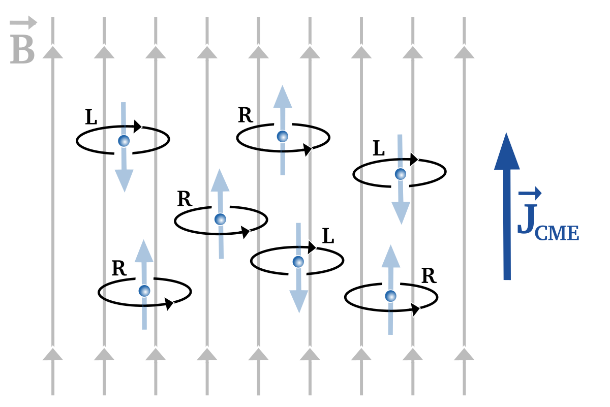
Figure 1: Illustration of the chiral magnetic effect. In the presence of an external magnetic field $\bm{B}$, the momenta of right-(left-)handed fermions at the lowest Landau level align with (antiparallel to) the field lines. An asymmetry between the number densities of left- and right-handed particles results in a net electric current $\bm{J}_{\rm CME}$. (Colour online)

2.2 System of chiral MHD equations

The chiral electric current (2) adds to the classical Ohmic current, leading to a modification of the Maxwell equations. Combining these equations with Ohm’s law, the following set of chiral MHD equations for an isothermal high temperature plasma is obtained:

$$\frac{\upartial\bm{B}}{\upartial t} = \bm{\nabla}\times\left[{\bm{U}}\times{\bm{B}}-\eta\,\left(\bm{\nabla}\times{\bm{B}}-\mu_{5}{\bm{B}}\right)\right],$$ (3)

$$\rho{{\mathrm{D}}\bm{U}\over{\mathrm{D}}t} = (\bm{\nabla}\times{\bm{B}})\times\bm{B}-\bm{\nabla}p+\bm{\nabla}{\bm\cdot}(2\nu\rho\mbox{\boldmath${\sf S}$}{})+\rho\bm{f},$$ (4)

$$\frac{{\mathrm{D}}\rho}{{\mathrm{D}}t} = -\rho\,\bm{\nabla}\cdot\bm{U},$$ (5)

$$\frac{{\mathrm{D}}\mu_{5}}{{\mathrm{D}}t} = D_{5}\,\Delta\mu_{5}+\lambda\,\eta\,\left[{\bm{B}}{\bm\cdot}(\bm{\nabla}\times{\bm{B}})-\mu_{5}{\bm{B}}^{2}\right]-C_{5}({\bm{B}}{\bm\cdot}\bm{\nabla})\mu-\Gamma_{\rm\!f}\mu_{5},$$ (6)

$$\frac{{\mathrm{D}}\mu}{{\mathrm{D}}t} = D_{\mu}\,\Delta\mu-C_{\mu}(\bm{B}{\bm\cdot}\bm{\nabla})\mu_{5},$$ (7)

where the magnetic field $\bm{B}$ is normalised such that the magnetic energy density is $\bm{B}^{2}/2$ (so the magnetic field in Gauss is $\sqrt{4\pi}\,\bm{B}$), $\eta$ is the magnetic resistivity, $\bm{U}$ is the velocity, and ${\mathrm{D}}/{\mathrm{D}}t\equiv\upartial/\upartial t+\bm{U}\cdot\bm{\nabla}$. The normalised chiral chemical potential $\mu_{5}\equiv(4\alpha_{\rm em}/\hbar c)\mu_{5}^{\mathrm{phys}}$ is scaled such that it has the same units as a wavelength (inverse length); see also table 1. The chiral nonlinearity parameter is

$$\lambda=3\hbar c\left({8\alpha_{\rm em}\over k_{\rm B}T}\right)^{2},$$ (8)

where $T$ is the temperature, $k_{\rm B}$ is the Boltzmann constant and $c$ is the speed of light. The expression for $\lambda$ given above is valid for $k_{\rm B}T\gg{\rm max}(|\mu_{{}_{\rm L}}^{\mathrm{phys}}|,|\mu_{{}_{\rm R}}^{\mathrm{phys}}|)$, which holds for the description of the hot plasma in the early Universe. In a dense plasma, like within a neutron star where $k_{\rm B}T\ll{\rm max}(|\mu_{{}_{\rm L}}^{\mathrm{phys}}|,|\mu_{{}_{\rm R}}^{\mathrm{phys}}|)$, a dependence on the usual chemical potential $\mu^{\mathrm{phys}}\equiv\mu_{{}_{\rm R}}^{\mathrm{phys}}+\mu_{{}_{\rm L}}^{\mathrm{phys}}$ needs to be included (see, e.g. Kharzeev, 2014; Kharzeev et al., 2016; Dvornikov and Semikoz, 2015).

In equations (3)–(7), $p$ is the fluid pressure, ${\sf S}_{ij}={\textstyle{1\over 2}}(U_{i,j}+U_{j,i})-{\textstyle{1\over 3}}\delta_{ij}{\bm\nabla}{\bm\cdot}\bm{U}$ are the components of the trace-free strain tensor, where commas denote partial spatial differentiation, $\nu$ is the kinematic viscosity, and $\bm{f}$ is a forcing function used to drive turbulence in DNS. For an isothermal equation of state, the pressure $p$ is related to the mass density $\rho$ via $p=c_{\rm s}^{2}\rho$, where $c_{\rm s}$ is the isothermal sound speed. The last term in equation (6) describes the chiral flipping reactions at a rate $\Gamma_{\rm\!f}>0$. This rate characterises the flipping between left- and right-handed states of a fermion and becomes important at low temperatures, i.e. when the mass of the particles cannot be neglected anymore. Equation (7) describes the evolution of $\mu^{\mathrm{phys}}$, which is, in consistency with $\mu_{5}$, normalised as $\mu\equiv(4\alpha_{\rm em}/\hbar c)\mu^{\mathrm{phys}}$. Equation (7) for $\mu$ and equation (6) for $\mu_{5}$ have been derived by Gorbar et al. (2016) using chiral kinetic theory in the high-temperature limit. The evolution equations of $\mu_{5}$ and $\mu$ are coupled through the coupling parameters $C_{5}$ and $C_{\mu}$, respectively, and $D_{5}$ and $D_{\mu}$ are diffusion coefficients.

Table 1: Physical units in chiral MHD

Parameter	cgs unit	Natural unit	Comment
$\mu_{5}^{\mathrm{phys}}$	erg	eV
$\mu_{5}$	$\mathrm{cm}^{-1}$	eV	$\mu_{5}=4\alpha_{\rm em}/(\hbar c)\mu_{5}^{\mathrm{phys}}$
$\mu^{\mathrm{phys}}$	erg	eV
$\mu$	$\mathrm{cm}^{-1}$	eV	$\mu=4\alpha_{\rm em}/(\hbar c)\mu^{\mathrm{phys}}$
$\lambda$	$\mathrm{s}^{2}\mathrm{g}^{-1}\mathrm{cm}^{-1}$	$\mathrm{eV}^{-2}$
$D_{5}$	$\mathrm{cm}^{2}\mathrm{s}^{-1}$	$\mathrm{eV}^{-1}$
$D_{\mu}$	$\mathrm{cm}^{2}\mathrm{s}^{-1}$	$\mathrm{eV}^{-1}$
$\sqrt{4\pi}\bm{B}$	G=$\mathrm{g}^{1/2}\mathrm{cm}^{-1/2}\mathrm{s}^{-1}$	$\mathrm{eV}^{2}$	defined such that $\bm{B}^{2}/2$ is an energy density
$\Gamma_{\mathrm{f}}$	$\mathrm{s}^{-1}$	$\mathrm{eV}$

In the Pencil Code, a dimensionless form of the system of equations (3)–(7) has been implemented. We give this system of equations in Appendix A. In the following we will use the chiral velocity, defined as $v_{\mu}\equiv\eta\mu_{5,0}$, where $\mu_{5,0}\equiv\mu_{5}(t=0)$, and the corresponding dimensionless chiral Mach number ${\rm Ma}_{\mu}\equiv v_{\mu}/c_{\mathrm{s}}$. Since $\mu_{5}$ has the dimension of a wavenumber (see also table 2), $v_{\mu}$ has the dimension of a velocity. Also, we introduce a dimensionless form of the chiral nonlinearity parameter as $\lambda_{5}=\lambda\eta^{2}\overline{\rho}$, where the overbar denotes a volume average. We note that the default setup of the Pencil Code does not include the $\mu$ terms and equation (7). These terms can be switched on via the logical parameter lmuS. If lmuS=.true., the MVAR CONTRIBUTION in cparam.local needs to be increased by one.

2.3 Conservation law in chiral MHD

A remarkable consequence of the system of equations (3)–(7) is that

$$\frac{\upartial}{\upartial t}\left({\lambda\over 2}{\bm A}{\bm\cdot}\bm{B}+\mu_{5}\right)+\bm{\nabla}{\bm\cdot}\left[{\lambda\over 2}\left({\bm\bm{E}}\times{\bm A}-\bm{B}\,\Phi\right)-D_{5}\bm{\nabla}\mu_{5}+C_{5}{\bm{B}}\mu\right]=0,$$ (9)

where $\bm{E}=-\bm{U}\times\bm{B}+\eta\bm{\nabla}\times\bm{B}-\eta\,\mu_{5}\,\bm{B}+{\rm O}(\eta^{2})$ is the electric field and ${\bm A}$ is the magnetic vector potential, with $\bm{B}=\bm{\nabla}\times{\bm A}$; see Boyarsky et al. (2012) and Section 4.3. of Rogachevskii et al. (2017). For periodic boundary conditions, which are often applied in MHD simulations, the divergence term in equation (9) vanishes and hence $\lambda{\bm A}{\bm\cdot}\bm{B}+2\mu_{5}=\mathrm{const}$. We stress that conservation of the sum of magnetic helicity density and chiral density holds for arbitrary values of $\eta$. This is different from classical MHD, where magnetic helicity $\int{\bm A}{\bm\cdot}\bm{B}\,dV$ is only conserved in the limit of $\eta\to 0$.

From equation (9), under the assumption of vanishing initial magnetic helicity, a maximum magnetic field strength for a given initial chiral chemical potential can be estimated through (Brandenburg et al., 2017)

$$\overline{\bm{B}^{2}}_{\mathrm{sat}}\,\xi_{\rm M}\approx{2\mu_{5,0}}\big{/}{\lambda},$$ (10)

where $\xi_{\rm M}$ is the correlation length of the magnetic field and overlines denote volume averages.

2.4 Length and time scales in chiral MHD

2.4.1 Laminar dynamo phase

With a plane wave ansatz, the linearised induction equation (3) with the CME term and a vanishing velocity field yields an instability that is characterized by the growth rate

$$\gamma(k)=|v_{\mu}k|-\eta k^{2},$$ (11)

with $k$ being the wavenumber. The maximum growth rate of this instability is

$$\gamma_{\mu}={v_{\mu}^{2}}\big{/}{(4\eta)},$$ (12)

and the typical wavenumber of the dynamo instability in laminar flows is

$$k_{\mu}={|\mu_{5}|}\big{/}{2}.$$ (13)

This chiral instability is caused by the term $\bm{\nabla}\times(v_{\mu}\bm{B})$ in the induction equation (3) of chiral MHD. We note that, while this term is formally similar to the $\alpha$ effect in classical mean-field MHD, the $v_{\mu}$ is not produced by turbulence, but rather by a quantum effect related to the handedness of fermions. This is the $v_{\mu}^{2}$ dynamo. In the presence of shear, its growth rate is modified in ways that are similar to those of the classical $\alpha\Omega$ dynamo (Rogachevskii et al., 2017), except that this chiral dynamo is not related to a turbulent flow.

2.4.2 Turbulent dynamo phase

In the presence of turbulence, regardless of whether it is driven by a forcing function or by the Lorentz force, the growth rate of the mean magnetic field obtained in the framework of the mean-field approach (Rogachevskii et al., 2017), is given by

$$\gamma(k)=|(\overline{v}_{\mu}+\alpha_{\mu})\,k|-(\eta+\,\eta_{{}_{T}})\,k^{2},$$ (14)

with $k^{2}=k_{x}^{2}+k_{z}^{2}$ and $\overline{v}_{\mu}$ being the mean chiral chemical potential multiplied by $\eta$. In comparison to equation (11), turbulent diffusion $\eta_{{}_{T}}=u_{\mathrm{rms}}/(3k_{\mathrm{f}})$ adds to Ohmic diffusion, where $k_{\mathrm{f}}$ is the forcing wavenumber. Additionally, as has been shown by Rogachevskii et al. (2017), the CME leads to a novel large-scale dynamo that is caused by the $\alpha_{\mu}$ effect:

$$\alpha_{\mu}=\begin{cases}-\dfrac{(q-1)}{3(q+1)}\,{\rm Re}_{{}_{\mathrm{M}}}^{2}\,\overline{v}_{\mu},&\mathrm{for}~{}{\rm Re}_{{}_{\mathrm{M}}}\ll 1,\\[8.00003pt] -\dfrac{2}{3}\overline{v}_{\mu}\log\,{{\rm Re}_{{}_{\mathrm{M}}}},&\mathrm{for}~{}{\rm Re}_{{}_{\mathrm{M}}}\gg 1,\end{cases}$$ (15)

with $1<q<3$. ${\rm Re}_{{}_{\mathrm{M}}}=u_{\mathrm{rms}}/(\eta k_{\mathrm{f}})$ is the magnetic Reynolds number. The expression given in equation (15) is valid for weak mean magnetic fields, when the energy of the mean magnetic field is much smaller than the turbulent kinetic energy. While $\alpha_{\mu}$ is related to the fluctuations of the magnetic and velocity field – in contrast to the $\alpha$ effect in classical mean-field MHD – kinetic helicity is not required for it to occur.

The maximum growth rate of the mean magnetic field is

$$\gamma_{\alpha}={(\overline{v}_{\mu}+\alpha_{\mu})^{2}\over 4(\eta+\,\eta_{{}_{T}})}={(\overline{v}_{\mu}+\alpha_{\mu})^{2}\over 4\eta(1+\,{\rm Re}_{{}_{\mathrm{M}}}/3)}.$$ (16)

The maximum growth rate of the $\alpha_{\mu}$ dynamo is attained at the wavenumber

$$k_{\alpha}={|\overline{v}_{\mu}+\alpha_{\mu}|\over 2(\eta+\,\eta_{{}_{T}})}={|\overline{v}_{\mu}+\alpha_{\mu}|\over 2\eta\,(1+\,{\rm Re}_{{}_{\mathrm{M}}}/3)}.$$ (17)

provided that small-scale turbulence is present.

There is one more characteristic scale in chiral MHD turbulence, namely the scale on which dynamo saturation occurs. It has been shown in Brandenburg et al. (2017) that, without applying a forcing function in the Navier-Stokes equation, the CME produces chiral-magnetically driven turbulence, which causes a $k^{-2}$ magnetic energy spectrum between the wavenumbers $k_{\mu}$ and

$$k_{\lambda}\approx 4\sqrt{\overline{\rho}\lambda}\,\mu_{5,0}\eta.$$ (18)

Regarding spatial scales, we note that a fluid description, as presented here, is only valid as long as all relevant chiral length scales are larger than the mean free path. Otherwise, a kinetic description of the plasma (Artsimovich and Sagdeev, 1985) needs to be applied, which will not be discussed here.

3 Application of the chiral MHD module in the Pencil Code

3.1 Implementation

In comparison to classical MHD, in chiral MHD the evolution equation of at least one additional scalar field, the chiral chemical potential $\mu_{5}(\boldsymbol{x},t)$, needs to be solved. The evolution equation for $\mu_{5}(\boldsymbol{x},t)$ is given by equation (6). Additionally, $\mu_{5}(\boldsymbol{x},t)$ enters the induction equation (3) via the chiral dynamo term $\bm{\nabla}\times(\eta\mu_{5}\bm{B})$.

Chiral MHD is currently implemented in the Pencil Code as a special module, where $\mu_{5}(\mathbf{x},t)$ is made available as a pencil p%mu5 and in the f-array, and can be activated by adding the line

   SPECIAL   =   special/chiral_mhd

to the file src/Makefile.local. Obviously, also the magnetic.f90 module needs to be switched on. For solving the complete set of equations (3)–(7), additionally, the hydro.f90 module, the density.f90 module, and an equation of state module are required. An example for the setup in the Pencil Code is presented in the appendix.

3.2 Time stepping

The time step $\delta t$ in the Pencil Code can either be set to a fixed value or be adjusted automatically, depending on the instantaneous values of characteristic time scales in the simulation. In the latter case, $\delta t$ is specified by the Courant time step, which is taken as the minimum of all involved terms of the equations solved in the simulation and can be multiplied by a user-definable scale factor cdt in the input file run.in.

The chiral-mhd.f90 module introduces the following six time step contributions:

$$\delta t_{\lambda_{5}}=\, \frac{1}{\lambda\eta\bm{B}^{2}},\, \delta t_{D_{5}}=\, \frac{\delta x^{2}}{D_{5}},\, \delta t_{\Gamma_{\mathrm{f}}}=\, \frac{1}{\Gamma_{\mathrm{f}}},$$ (19)

$$\hskip 42.67912pt\delta t_{\mathrm{CMW}}=\, \frac{\delta x}{|\bm{B}|\sqrt{C_{5}C_{\mu}}},\, \delta t_{D_{\mu}}=\, \frac{\delta x^{2}}{D_{\mu}},\, \delta t_{v_{\mu}}=\, \frac{\delta x}{\eta\mu_{5}}.\hskip 56.9055pt$$ (20)

The contribution $\delta t_{\lambda_{5}}$ results from the term proportional to $\lambda$ in equation (6) and $\delta t_{\Gamma_{\mathrm{f}}}$ from the flipping term in the same equation. The contributions $\delta t_{D_{5}}$ and $\delta t_{D_{\mu}}$ are required to describe diffusion of $\mu_{5}$ and $\mu$, respectively. Further, $\delta t_{v_{\mu}}$ results from the chiral dynamo term in the induction equation and $\delta t_{\mathrm{CMW}}$ from chiral magnetic waves (CMWs). The total contribution to the time step calculated in the chiral MHD module, is given by

$$\delta t_{\mathrm{chiral}}=c_{\mathrm{\delta t,chiral}}~{}\mathrm{min}(\delta t_{\lambda_{5}},\delta t_{D_{5}},\delta t_{\Gamma_{\mathrm{f}}},\delta t_{\mathrm{CMW}},\delta t_{D_{\mu}},\delta t_{v_{\mu}}),$$ (21)

which can be scaled by the parameter $c_{\mathrm{dt,chiral}}$. The default value of $c_{\mathrm{dt,chiral}}$ is chosen to be unity, but can be set to smaller values in run.in.

The relative importance of the chiral contributions to the simulation time step is demonstrated in figure 2, where four different simulations are presented. These simulations are performed in two-dimensional (2D) domains with a size of $(2\pi)^{2}$ and a resolution of $512^{2}$, that is, $\delta x\approx 0.012$, and the magnetic and chiral Prandtl numbers are ${\rm Pr}_{{}_{\mathrm{M}}}=\nu/\eta=1$ and ${\rm Pr}_{{}_{5}}=\nu/D_{5}=1$, respectively; see also appendix A. We probe different combinations of the chiral Mach number, using ${\rm Ma}_{\mu}=0.5$ and $2$, and the nonlinearity parameter $\lambda_{5}=0.5$ and $8$, as given in the individual panels of figure 2. In these examples, the chiral flipping rate and the chemical potential have been neglected. We note that this might be an incorrect simplification for proto-neutron stars, where $\Gamma_{\mathrm{f}}$, being proportional to $m_{e}^{2}$, can reach very large values (Grabowska et al., 2015; Dvornikov, 2017). DNS with non-vanishing $\Gamma_{\mathrm{f}}$ have been presented in Schober et al. (2018b), where it was shown that the evolution of $\mu_{5}$, and hence $B_{\mathrm{rms}}$, can be strongly affected in the case without turbulence. A detailed study of the effect of chiral flipping reactions in a turbulent plasma and the potential damping out of chiral magnetic instabilities, will be an interesting subject for future DNS.

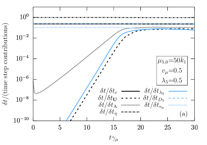
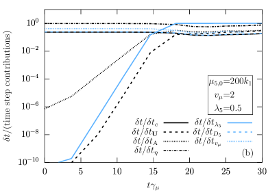
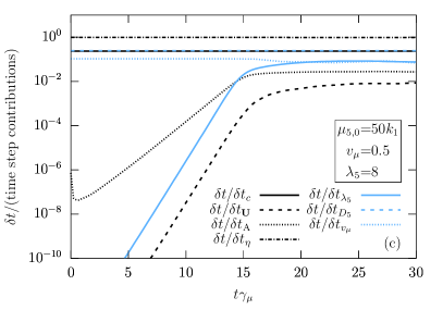
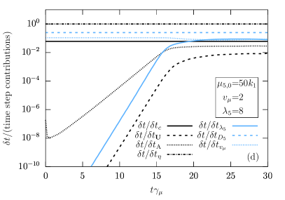
Figure 2: Comparison of various contributions to the time step. Different panels show 2D simulations with different values of $\mu_{5,0}/k_{1}$, $v_{\mu}$, and $\lambda_{5}$ as indicated in the boxes. In all cases, ${\rm Pr}_{{}_{\mathrm{M}}}={\rm Pr}_{{}_{5}}=1$ and the resolution is $512^{2}$ mesh points. Different lines show different time steps, where black colour indicates time steps from classical MHD and blue colour shows time steps from the chiral MHD module. The time steps are normalised by the overall $\delta t$, which is determined as the minimum of the individual time steps from all term involved. (Colour online)

In typical simulations of chiral MHD, the minimum time step is not determined by the new contributions from the chiral_mhd.f90 module, but those can have an important indirect effect caused by the amplification of the magnetic field. It can be seen from figure 2 that the chiral contributions, indicated by blue colour, play mostly a subdominant role. For comparison, time-step contributions from classical MHD are plotted, including the acoustic time-step $\delta t_{c}=c_{\delta t}\delta x/\mathrm{max}(c_{\mathrm{s}})$, the advective time-step $\delta t_{\bm{U}}=c_{\delta t}\,\delta x/{\rm max}|\bm{U}|$, the Alfvén time-step $\delta t_{\mathrm{A}}=c_{\delta t}\,\delta x/{\rm max}|v_{\mathrm{A}}|$, and the resistive time-step $\delta t_{\eta}=c_{\delta t,\mathrm{v}}\,\delta x^{2}/\eta$, where $c_{\delta t}$ and $c_{\delta t,\mathrm{v}}$ are user-defined constants (the default values are $c_{\delta t}=0.9$ and $c_{\delta t,\mathrm{v}}=0.25$), and $v_{\mathrm{A}}$ is the Alfvén velocity. From equations (19) and (20), one could get the impression that the chiral time step should become very small when the magnetic field is strong, that is, at dynamo saturation. However, $\bm{B}^{2}$ occurs here always with a prefactor of $\lambda$ and, according to equation (10), $\bm{B}^{2}\lambda\approx\mu_{5,0}$. The only regime where the chiral contribution to the time step becomes important is the nonlinear phase of a plasma with large $v_{\mu}$ and low $\lambda_{5}$; e.g. for $t\gamma_{\mu}>17$ in figure 2(b).

Increasing ${\rm Ma}_{\mu}$ has an effect on the contributions to the time step from classical MHD. As mentioned before, a larger $\mu_{5,0}$ leads to a larger saturation magnetic field strength; see equation (10). This increases the Alfvén velocity and reduces the corresponding time step, $\delta t_{\mathrm{A}}$; see the evolution of the black dotted lines in figure 2.

3.3 Minimum resolution

The minimum resolution required for a simulation can be estimated using the mesh Reynolds number, which is defined as

$$\mbox{Re}_{\rm mesh}=\frac{{\rm max}(|\bm{U}|)\delta x}{\nu},$$ (22)

based on the resolution $\delta x$. The value of $\mbox{Re}_{\rm mesh}$ should not exceed a certain value, which is approximately $5$, but can be larger or smaller, depending on the nature of the flow (smaller when the flow develops shocks, for example); see the Pencil Code manual, section K.3. Using this empirical value for a given viscosity (or resistivity) and given maximum velocity, a minimum resolution $\delta x$ can be estimated.

In the following, velocities are given in units of the speed of sound, $c_{\mathrm{s}}$. Besides the sound speed, the turbulent velocity and shear velocities can occur and determine $\mbox{Re}_{\rm mesh}$. Most importantly at late stages of chiral dynamo simulations, i.e., in the nonlinear dynamo phase and especially close to saturation, the Alfvén velocity, $v_{\mathrm{A}}$, can play a dominant role. In dimensional units, $v_{\mathrm{A,rms}}=B_{\mathrm{rms}}/\sqrt{\overline{\rho}}$, but in code units with $\overline{\rho}=1$, we have $v_{\mathrm{A,rms}}=B_{\mathrm{rms}}$.

In chiral MHD, the maximum $v_{\mathrm{A}}$ can be estimated from the conservation law (9). Assuming that the magnetic field has a correlation length that is equal to the size of the domain, the maximum magnetic field is of the order of $(\mu_{5,0}/\lambda)^{1/2}$; see equation (10). Hence, when a domain of size $(2\pi)^{3}$ is resolved with $N_{\mathrm{grid}}^{3}$ grid points, we find the following requirement for the minimum resolution:

$$N_{\mathrm{grid}}\gtrsim\left(\frac{\mu_{5,0}}{\lambda}\right)^{1/2}\frac{2\pi}{\nu\mbox{Re}_{\rm mesh,crit}}.$$ (23)

One must not use too large values of mu5_const in start.in and too small values of nu (or eta) and lambda5 in run.in. For example, when $\mu_{5,0}=10$, $\lambda=10^{3}$ and $\nu=10^{-3}$, a resolution of more than $128^{3}$ mesh points is necessary.

We note that, in principle, larger saturation values of the magnetic field can be calculated in the Pencil Code by manually setting the value of $c_{\mathrm{s}}$ in start.in to a larger value, e.g. $c_{\mathrm{s}}=2$. This, however, is accompanied by a decrease of the simulation time step; see the previous section.

4 Numerical simulations in chiral MHD

4.1 The chiral MHD dynamo instability

4.1.1 Classical vs. chiral MHD

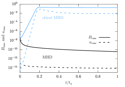
Figure 3: Classical vs. chiral MHD. Two 2D simulations with a an initially weak magnetic field and vanishing velocity field, without external forcing of turbulence. The black lines show the evolution of the rms magnetic fields strength (solid black line) and the rms velocity (dashed black line) in the case of classical MHD. Here both, $B_{\mathrm{rms}}$ and $u_{\mathrm{rms}}$, decay in time, which is plotted in terms of the resistive time, $t_{\eta}\equiv{(\eta k_{1})^{-1}}$. When the chiral chemical potential is non-zero, as here shown with blue colour, both, $B_{\mathrm{rms}}$ and $u_{\mathrm{rms}}$, grow exponentially over many orders of magnitude, due to the laminar chiral MHD dynamo. (Colour online)

The term $\bm{\nabla}\times(\eta\mu_{5}\bm{B})$ in the induction equation (3) drastically increases the range of laminar and turbulent dynamos. An example, where the evolution of a plasma with CME differs strongly from the classical picture, is presented in figure 3. The two 2D runs in domains of size $(2\pi)^{2}$ compared there, are resolved by $256^{2}$ grid cells. They have periodic boundary conditions, an initially vanishing velocity field, and a weak magnetic seed field. In both cases, ${\rm Pr}_{{}_{\mathrm{M}}}=\mathrm{Pr}_{5}=1$, explicit viscosity, resistivity, and diffusivity of $\mu_{5}$ have been included, and the equation of state is that of an ideal gas.

The run presented as black lines in figure 3 shows the classical MHD case. Here, as expected, the magnetic field decreases, since no classical dynamo is operating in this system. The blue lines in figure 3 show the time evolution for a typical chiral MHD scenario. The simulation setup is chosen exactly in the same way as for the classical MHD case, with the exception that the chiral_mhd.f90 module is activated, that is, the induction equation includes the term $\bm{\nabla}\times(\eta\mu_{5}\bm{B})$ and equation (6) is solved to follow the evolution of $\mu_{5}$. The simulation parameters are chosen such that ${\rm Ma}_{\mu}=0.02$ and $\lambda_{5}=0.002$. The chiral instability scale is equal to $\mu_{5,0}/k_{1}=20$, where $k_{1}=1$ is the largest wavenumber possible in the numerical domain.

The instability caused by the chiral term in the induction equation leads to an increase of $B_{\mathrm{rms}}$ over more than 6 orders of magnitude before saturation commences. This occurs after less than $0.2$ diffusive times, $t_{\eta}$. Simultaneously, the velocity $u_{\mathrm{rms}}$ increases by approximately 12 orders of magnitude due to driving of turbulence via the Lorentz force, that is, via chiral-magnetic driving.

4.1.2 Initial conditions for the chiral MHD dynamo

Laminar dynamo theory predicts a scale-dependent growth rate of the magnetic field according to equation (12). If the initial magnetic field is distributed over all wavenumbers within the box, like, for example, in case of Gaussian noise, the instability is strongest on the scale $k_{\mu}=\mu_{5,0}/2$ and the rms magnetic field strength $B_{\mathrm{rms}}$ grows at the maximum rate $\gamma_{\mu}=\eta\mu_{5,0}^{2}/4$. If the initial magnetic field is, however, concentrated at a single wavenumber $k_{\mathrm{B}}$, which is the case for a force-free Beltrami field, e.g., for a vector potential $\bm{A}=(\cos k_{\mathrm{B}}z,\;\sin k_{\mathrm{B}}z,\;0)$, $B_{\mathrm{rms}}$ increases at the rate $\gamma(k_{\mathrm{B}})$.

A demonstration of the importance of the initial magnetic field configuration is presented in figure 4, which shows the time evolution for three 2D simulations. All of these simulations have $k_{\mu}/k_{1}=10$. The case with initial Gaussian noise increases with $\gamma_{\mu}$ until saturation is reached at approximately $t=0.2~{}t_{\eta}$. The Beltrami field, initiated at wavenumber $k_{\mathrm{B}}=1$, grows at a rate $\gamma(1)<\gamma_{\mu}$. Only once a field strength of $\eta^{2}\mu_{5,0}$ at $t\approx 0.4~{}t_{\eta}$ is reached, the field configuration has changed sufficiently such that the magnetic energy is non-zero at $k_{\mu}$ and the $B_{\mathrm{rms}}$ continues to grow with $\gamma_{\mu}$.

We note that a Beltrami initial field can also result in amplification with $\gamma_{\mu}$, if it is concentrated around $k_{\mathrm{B}}=k_{\mu}$. This is demonstrated by the simulation with $k_{\mathrm{B}}=k_{\mu}=20~{}k_{1}$, which increases with the maximum possible growth rate from the beginning. For all runs discussed above, the growth rates are shown in figure 4(b) as a function of time.

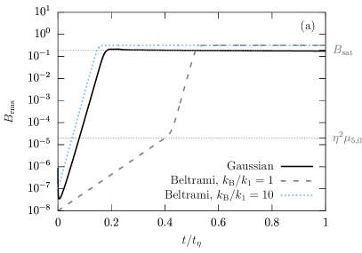
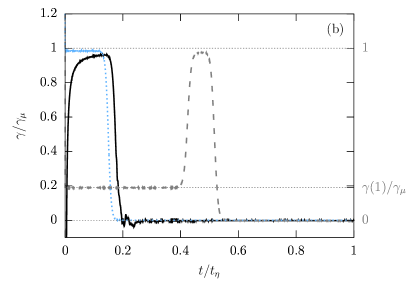
Figure 4: Simulations with different initial conditions of the magnetic field. The 2D simulations with a domain of $(2\pi)^{2}$ and a resolution of $256^{2}$ have parameters of ${\rm Pr}_{{}_{\mathrm{M}}}=1$, $\lambda_{5}=0.002$, and $k_{\mu}/k_{1}=10$. The runs differ in the configurations of the initial magnetic field. We consider Gaussian noise (black solid lines) and Beltrami fields with $k_{\mathrm{B}}/k_{1}=1$ (gray dashed lines) and $k_{\mathrm{B}}/k_{1}=k_{\mu}/k_{1}=10$ (blue dotted lines). (a) Time evolution of the rms magnetic field strength. (b) Time evolution of the growth rate of the magnetic field strength. (Colour online)

4.2 Chiral MHD in turbulence

4.2.1 Properties of chiral dynamos in chiral-magnetically and externally driven turbulence

The effects of turbulence on the evolution of a magnetic field in a chiral plasma can be described by mean-field theory, which was reviewed briefly in Section 2.4.2. The Pencil Code allows for more detailed studies of chiral turbulent dynamos without using simplifications of the equations that are made for an analytical treatment. Therefore, in the following we present two three-dimensional simulations in domains of size $(2\pi)^{3}$ with periodic boundary conditions and a resolution of $200^{3}$. They are initiated with a weak random magnetic field and a chiral chemical potential $\mu_{5,0}=20k_{1}$. The two DNS are identical except for the fact that in one, turbulence is driven externally at the wavenumber $k_{\rm f}=10\,k_{1}$. We label the run with external forcing as “$\mathrm{R}_{\mathrm{f}}$”, where “f” refers to forcing, and the initially laminar one as “$\mathrm{R}_{\chi}$”, where “$\chi$” refers to chiral-magnetically driven turbulence.

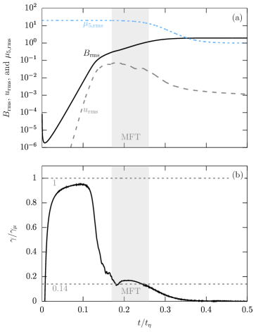
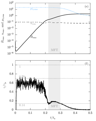
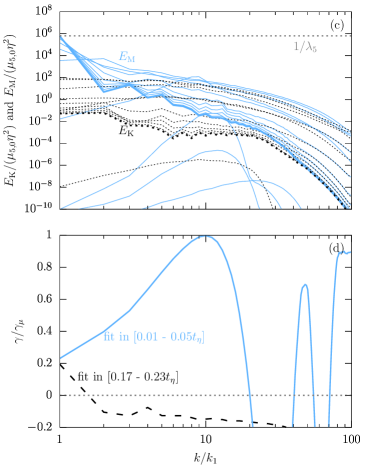
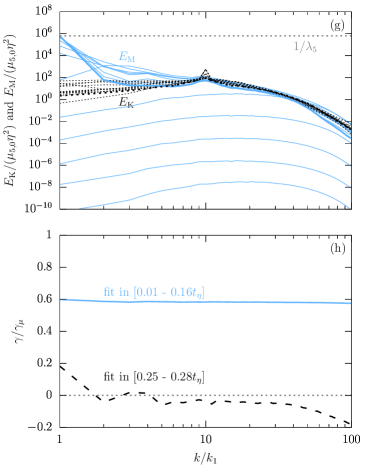
Figure 5: Direct comparison of chiral MHD dynamos in chiral-magnetically driven turbulence (left) and externally forced turbulence (right). In the first two rows, we present the time series of $B_{\mathrm{rms}}$, $u_{\mathrm{rms}}$, $\mu_{5,\mathrm{rms}}$, and $\gamma/\gamma_{\mu}$. The time interval in which linear mean-field theory (“MFT”) applies is highlighted by a gray background. In the third row, the dotted black lines show kinetic energy spectra and the solid blue lines show magnetic energy spectra in uniform time intervals. The final spectra, obtained at $t=0.5t_{\eta}$ are plotted as thick lines. The scale dependence of the growth rate at different time intervals is shown in the last line. (Colour online)

In figure 5, the two simulations are compared directly, where we present run $\mathrm{R}_{\chi}$ in the left panels and run $\mathrm{R}_{\mathrm{f}}$ in the right panels. The main differences between the two cases are clearly visible in the upper panels, which show the time evolution of $B_{\mathrm{rms}}$, $u_{\mathrm{rms}}$, and $\mu_{5,\mathrm{rms}}$. The magnetic field grows much faster in run $\mathrm{R}_{\chi}$, which can be seen more clearly in the second row of figure 5, where the evolution of $\gamma$, normalised by the laminar growth rate $\gamma_{\mu}$, is presented. Simultaneously with $B_{\mathrm{rms}}$ growing at a rate of $\gamma_{\mu}$, $u_{\mathrm{rms}}$ grows at a rate of approximately $2\gamma_{\mu}$, as expected for driving through the Lorentz force. Once the kinetic energy becomes comparable to the magnetic energy at $t\approx 0.12~{}t_{\eta}$, $\gamma$ decreases as a result of additional turbulent diffusion. When turbulence is forced externally, we observe an initial amplification of $B_{\mathrm{rms}}$ with a growth rate that is reduced as compared to $\gamma_{\mu}$. As in run $\mathrm{R}_{\chi}$, mean-field effects, e.g. turbulent diffusion and the $\alpha_{\mu}$ effect, occur in $\mathrm{R}_{\mathrm{f}}$ once $B_{\mathrm{rms}}\approx u_{\mathrm{rms}}$, resulting in an overall decrease of the growth rate at $t\approx 0.2~{}t_{\eta}$.

A major difference between externally and chiral-magnetically driven turbulence appears in the comparison of the energy spectra; see the third row of figure 5. While in the initially laminar run $\mathrm{R}_{\chi}$, the magnetic field instability occurs at wavenumber $k_{\mu}=\mu_{5,0}/2=10$, we observe a scale-independent growth of the magnetic energy in $\mathrm{R}_{\mathrm{f}}$. The growth rate is presented as a function of $k$ in the bottom panel. This dependence is clearly different from the parabola shape predicted from theory, see equation (11), and is the result of mode coupling. Hence, in the presence of turbulence, the magnetic field grows at a reduced rate, which can be estimated

as

$$\tilde{\gamma}(\mu_{5,0})=\frac{1}{\mu_{5,0}-k_{1}}\int_{k_{1}}^{\mu_{5,0}}\gamma(k)~{}\mathrm{d}k=\, \frac{1}{6}\eta(\mu_{5,0}-k_{1})(\mu_{5,0}+2k_{1})$$

$$=\, \frac{2}{3}\frac{(\mu_{5,0}-k_{1})(\mu_{5,0}+2k_{1})}{\mu_{5,0}^{2}}\gamma_{\mu}.$$ (24)

The value $\tilde{\gamma}(\mu_{5,0})$ reaches its maximum of $(3/4)\gamma_{\mu}$ at $\mu_{5,0}=4k_{1}$. When $\mu_{5,0}$ is increased, the initial growth rate of the magnetic field decreases; e.g. for $\mu_{5,0}=20k_{1}$ we find $\tilde{\gamma}(20k_{1})\approx 0.70\gamma_{\mu}$, as expected for our DNS, and for $\mu_{5,0}=100k_{1}$ we estimate $\tilde{\gamma}(100k_{1})\approx 0.67\gamma_{\mu}$. The growth rate of $0.70\gamma_{\mu}$ is indicated as a horizontal dotted line in figure 5(f).

In runs $\mathrm{R}_{\chi}$ and $\mathrm{R}_{\mathrm{f}}$, the presence of an $\alpha_{\mu}$ effect, which drives a large-scale dynamo, can only be seen at late times, shortly before dynamo saturation. As discussed in Schober et al. (2018b) and in the following section in more detail, the growth rates measured in DNS at late times agree approximately with the theoretical prediction from equation (16).

The DNS results suggest that mean-field effects in the evolution of the magnetic field occur once the magnetic energy is larger than the kinetic energy. In terms of normalised quantities, this translates to $B_{\mathrm{rms}}>u_{\mathrm{rms}}$. Whether or not the system can reach this condition is determined by the chiral conservation law and, in particular, by the value of $\lambda$. Using equation (10), one finds that mean-field effects in the evolution of $B_{\mathrm{rms}}$ occur for $\lambda\lesssim\mu_{5,0}/(\xi_{\mathrm{M}}u_{\mathrm{rms}}^{2})$.

4.2.2 Indirect evidence for the $\alpha_{\mu}$ effect

In the limit of large ${\rm Re}_{{}_{\mathrm{M}}}$ and a weak mean magnetic field, the theoretically expected growth rate (16) can be written as

$$\gamma_{\alpha}({\rm Re}_{{}_{\mathrm{M}}})=\gamma_{\mu}\frac{\left[1-(2/3)\,\log\,{\rm Re}_{{}_{\mathrm{M}}}\right]^{2}}{1+\,{\rm Re}_{{}_{\mathrm{M}}}/3}.$$ (25)

In fact, at ${\rm Re}_{{}_{\mathrm{M}}}\approx 4.5$, $\gamma_{\alpha}({\rm Re}_{{}_{\mathrm{M}}})$ as given above vanishes. However, at these moderate values of ${\rm Re}_{{}_{\mathrm{M}}}$, deviations from the $\tau$ approximation, used for deriving equation (25), can be expected. The maximum of the dynamo growth rate in turbulence is expected for ${\rm Re}_{{}_{\mathrm{M}}}\approx 38.7$, where $\gamma_{\alpha}(38.7)\approx 0.15\gamma_{\mu}$.

In the DNS presented in figure 5, the maximum Reynolds number for run $\mathrm{R}_{\chi}$ is $\approx 25$, which is comparable to the value of ${\rm Re}_{{}_{\mathrm{M}}}$ achieved in run $\mathrm{R}_{\mathrm{f}}$ via external forcing. Based on mean-field theory we expect $\gamma_{\alpha}(25)\approx 0.14\gamma_{\mu}$, which is indicated as horizontal dotted lines in figures 5(b) and 5(f). The agreement between the growth rate measured in DNS and mean-field theory, shown in these two examples, can be viewed as indirect evidence for the existence of the $\alpha_{\mu}$ effect.

4.3 MHD waves and the CME

The chiral asymmetry also affects the dispersion relation for MHD waves in a plasma. If a chiral instability is excited, it has a direct effect on the the frequencies and amplitudes of Alfvén and magnetosonic waves through the amplification of the magnetic field. How the dispersion relation in chiral MHD differs from the one in classical MHD has been shown in (Rogachevskii et al., 2017). The general expression for a compressible flow is given by

$$\left(\omega^{2}-\omega_{\rm A}^{2}\right)\,\Big{[}\omega^{4}-\omega^{2}\,({\bm v}_{A}^{2}+c_{\rm s}^{2})k^{2}+\omega_{\rm A}^{2}c_{\rm s}^{2}k^{2}\Big{]}-\omega^{2}\,(v_{\mu}\,k)^{2}\,\left(\omega^{2}-c_{\rm s}^{2}k^{2}\right)=0,$$ (26)

where $\omega_{\rm A}={\bm k}\cdot{\bm v}_{A}$ is the frequency of Alfvén waves in the absence of the CME. The complexity of the dispersion relation (26) indicates that in chiral MHD, the Alfvén and magnetosonic waves are strongly affected by a non-zero $\mu_{5}$. For solutions of equation (26) as a function of the angle between the wavevector ${\bm k}$ and the background magnetic field, we refer to figure 1 of Rogachevskii et al. (2017). In summary, the frequencies of the Alfvén wave and the magnetosonic wave are increased for a weak magnetic field, while the frequency of the slow magnetosonic wave is decreased in chiral MHD.

We use the Pencil Code to study the properties of MHD waves in chiral MHD. To this end, we set up 1D simulations with an imposed magnetic field of the form $(B_{0},0,0)$ and $B_{0}=0.1$. As initial condition for the magnetic field, we use Alfven-x, which creates an Alfvén wave travelling in the $x$ direction:

$$A_{z}\propto\sin(k_{x}x-\omega_{\rm A}t).$$ (27)

The simulations of a domain with an extension $[-\pi,\pi]$ are resolved by $128$ grid points and the magnetic Prandtl number is $1$.

In figure 6, the effect of changing $v_{\mu}$ on the propagation of the wave is illustrated. In the left panel, the classical MHD case with $v_{\mu}=0$ is shown for reference. Here the Alfvén wave is damped, leading to a decrease of the amplitude in time and a propagation of the peak to the right with the Alfvén velocity $v_{\mathrm{A}}$. In the middle panel, a chiral MHD run is shown with $v_{\mu}=0.2$ and in the right panel with $v_{\mu}=0.3$. In all panels of figure 6, we show the same time interval, and curves of the same colour indicate the same times. One clearly sees in these simulations that, in chiral MHD, the wave propagates more slowly, while its amplitude increases due to the chiral dynamo instability.

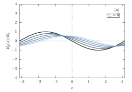
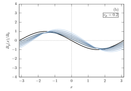
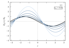
Figure 6: Propagation of a one-dimensional Alfvén wave for different values of $\boldsymbol{v_{\mu}}$. From left to right, $v_{\mu}$ increases from $0$ (classical MHD) to $v_{\mu}=0.3$. The black lines show the initial condition of $B_{y}$ ($t=0$) and later times are indicated by blue colour with the lightest blue indicating the last time shown in the figure ($t=0.16~{}t_{\mathrm{P}}$ with $t_{\mathrm{P}}$ being the period of a classical Alfvén wave). The time difference between neighbouring lines is constant and the magnetic field is normalised to its initial amplitude. (Colour online)

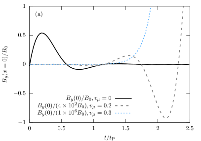
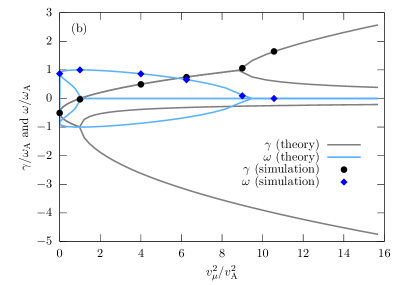
Figure 7: Effect of the CME on a one-dimensional Alfvén wave for different values of $\boldsymbol{v_{\mu}}$. (a) The displacement of $B_{y}/B_{0}$ in the middle of the one-dimensional domain (at $x=0$) for the three runs presented in figure 6. The black solid curve, with $v_{\mu}=0$, shows the classical damped Alfvén wave with the normal Alfvén frequency $\omega_{\mathrm{A}}$. For better visibility, we present the case of $v_{\mu}=0.2$ (gray dashed line) divided by a factor of $4\times 10^{2}$ and the case of $v_{\mu}=0.3$ (blue dotted line) divided by a factor of $10^{6}$. (b) Solution of the dispersion relation (26) and comparison with simulation results for runs with different $v_{\mu}$. Theoretical solutions for the growth rate $\gamma$ (real parts of solutions) are shown as gray lines and solution for the frequency $\omega$ (imaginary parts of solutions) as light blue lines. On top of these curves results from DNS with different values of $v_{\mu}$ are presented: Black dots show the measured growth rates and blue diamonds the frequencies, both of which are obtained from fits to $B_{y}(x=0,t)$. (Colour online)

In figure 7(a), we present the time evolution of $B_{y}(x=0)$ for all runs shown in figure 6. In the classical MHD case, the Alfvén wave is damped and the amplitude becomes indistinguishable from zero after approximately 1.5 periods. The case of $v_{\mu}=0.2$ corresponds to a wave with a growing amplitude. By contrast, for $v_{\mu}=0.3$ we observe a non-oscillating solution with exponentially growing amplitude. By fitting $B_{y}(x=0)$, we can obtain the growth rate $\gamma$ and the frequency $\omega$. The results of these fits are presented in figure 7(b) as a function of $(v_{\mathrm{A}}/v_{\mu})^{2}$. The values measured in DNS agree well with the solutions of the dispersion relation (26), which are presented as solid lines.

4.4 The role of the chemical potential

In all the simulations discussed up to now, the ordinary chemical potential $\mu$ has been neglected. For finite $C_{5}$, however, the evolution of $\mu_{5}$ is coupled to that of $\mu$ via the term $-C_{5}({\bm{B}}{\bm\cdot}\bm{\nabla})\mu$, which could potentially affect chiral MHD dynamos and excite collective modes. In this section we present DNS of chiral MHD including a non-zero chemical potential.

4.4.1 Effects on the nonlinear evolution of the chiral dynamos

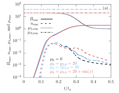
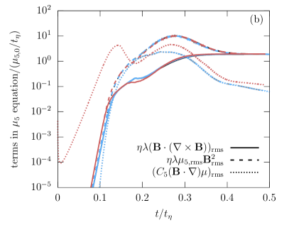
Figure 8: Chiral MHD dynamos with different chemical potentials $\boldsymbol{\mu}$. The figure shows results for various initial conditions with $\mu_{0}=0$ and $\mu_{5,0}=20$ (black lines), $\mu_{0}=\mu_{5,0}=20$ (grey lines), $\mu_{0}=2\mu_{5,0}=40$ (blue lines), and $\mu_{0}=\mu_{5,0}=20+\sin(x)$ (red lines). (a) Time evolution of $B_{\mathrm{rms}}$, $u_{\mathrm{rms}}$, $\mu_{5,\mathrm{rms}}$, and $\mu_{\mathrm{rms}}$, as indicated in the label. (b) Time evolution of the terms in the evolution equation of $\mu_{5}$, normalised to $\mu_{5,0}/t_{\eta}$. (Colour online)

To explore the role of the chemical potential in chiral dynamos, we repeat our exemplary run for chiral-magnetically driven turbulence, which is presented in figures 5(a)–(d). Here we solve the full system of equations (3)–(7), neglecting only the forcing term in the Navier-Stokes equation and chirality flipping in the evolution equation of $\mu_{5}$. The diffusivity $D_{\mu}$ has the same value as $D_{5}=\eta=\nu$ and for the coupling constants in equations (6) and (7) we use $C_{5}=C_{\mu}=1$, respectively. Three different initial conditions for the chemical potential are considered: $\mu_{0}=\mu_{5,0}=20k_{1}$, which illustrates the case with only left- or right-handed fermions, a case with $\mu_{0}=2\mu_{5,0}=40k_{1}$, and $\mu_{0}=\mu_{5,0}=(20+\sin(x))k_{1}$.

In figure 8(a), these three runs are compared with the simulation presented in figures 5(a)–(d), where $\mu_{0}=0$ and the evolution of $\mu$ has been neglected. Different colours in figure 8 indicate results for different runs. Black lines show the case presented in figure 5(a)–(d), grey lines the case where $\mu_{0}=\mu_{5,0}$, blue lines the case where $\mu_{0}=2\mu_{5,0}$, and red lines the case with a sinusoidal spatial variation in $\mu_{0}$ and $\mu_{5,0}$. As one may expect, only minor differences in the nonlinear phase of $u_{\mathrm{rms}}$ and $\mu_{5,\mathrm{rms}}$ can be noticed between the different runs. Naturally, the small deviations of $u_{\mathrm{rms}}$ and $\mu_{5,\mathrm{rms}}$ do not depend on the value of $\mu_{0}$ if it is constant and non-zero. A slightly larger change in the non-linear evolution of $u_{\mathrm{rms}}$ as compared to $\mu_{0}=0$, is seen in the case of an initial sinusoidal variation of $\mu_{0}$, due to the larger gradients in $\mu$.

For a better understanding of the evolution of $\mu_{5}$ in the different DNS, we present in figure 8(b) the time evolution of the various terms in equation for $\mu_{5}$: $\lambda\,\eta\,{\bm{B}}{\bm\cdot}(\bm{\nabla}\times{\bm{B}})$, $\lambda\,\eta\,\mu_{5}{\bm{B}}^{2}$, and $C_{5}({\bm{B}}{\bm\cdot}\bm{\nabla})\mu$. All of these terms are normalised by $\mu_{5,0}/t_{\eta}$ and the same colour code is used as in figure 8(a). It is important to note that the first two of these terms are only relevant for the nonlinear dynamo phase, e.g. when $\bm{B}$ is large. As can be seen in the plot, the term $\lambda\,\eta\,\mu_{5}{\bm{B}}^{2}$ is eventually responsible for decreasing $\mu_{5}$ and therefore shutting off the dynamo. We observe only very minor differences between all three runs in the terms $\lambda\,\eta\,{\bm{B}}{\bm\cdot}(\bm{\nabla}\times{\bm{B}})$ and $\lambda\,\eta\,\mu_{5}{\bm{B}}^{2}$. Obviously, the term $C_{5}({\bm{B}}{\bm\cdot}\bm{\nabla})\mu$ evolves very differently for a constant $\mu_{0}$ and one with a sinusoidal variation. Therefore the red dotted line is initially dominant. At time $\approx 0.12t_{\eta}$, it drops and the non-linear dynamo phase in this case becomes comparable to the cases with constant $\mu_{0}$. For extreme gradients in $\mu$, the term $C_{5}({\bm{B}}{\bm\cdot}\bm{\nabla})\mu$ could, in principle, suppress the mean-field chiral dynamo phase completely.

In summary, our DNS show that a non-zero constant initial $\mu$ does not affect chiral dynamos in the non-linear regime, and a very minor effect is observed if $\mu$ has an initial sinusoidal spatial variation. Yet, a systematic exploration of the parameter space and the impact of initial conditions on a chiral plasma, including the evolution of $\mu$, is beyond the scope of this paper.

4.4.2 Effects on collective modes

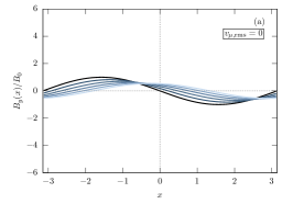
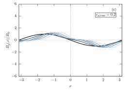
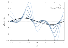
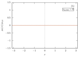
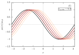
Figure 9: Propagation of a one-dimensional Alfvén wave for different values of $\boldsymbol{v_{\mu}}$ and with non-zero $\mu$. The top panels are the same as in figure 6 and in the bottom panels the propagation of the chiral magnetic wave is shown. The coupling constants in these runs are $C_{5}=C_{\mu}=1$. (Colour online)

A non-zero chemical potential $\mu$ can trigger chiral magnetic waves (CMWs; see Kharzeev and Yee, 2011), as described by the coupled linearised equations (6) and (7). The frequency of chiral magnetic waves is

$$\omega_{\rm CMW}=(C_{5}\,C_{\mu})^{1/2}\left|{\bm k}{\bm\cdot}{\bm B}_{0}\right|.$$ (28)

In order to explore these collective modes, we repeat the 1D runs of section 4.3 for a non-zero $\mu_{0}$. Again, the initial magnetic field is of the form (27) and we use

$$\mu_{5,0}=\mu_{5,0}^{A}\sin(k_{x}x)\quad\mathrm{and}\quad\mu_{0}=\mu_{0}^{A}\sin(k_{x}x).$$ (29)

Such an initial condition results in a chiral dynamo with an $x$-averaged absolute value of the chiral chemical potential $\mu_{5,\mathrm{rms},0}=2\mu_{5,0}^{A}/\pi$, due to the “quadratic” nature of the $v_{\mu}^{2}$ dynamo. All the DNS discussed in the following have $\mu_{0}^{A}=\mu_{5,0}^{A}$ and $C_{5}=C_{\mu}$.

In figure 9, we present results for $v_{5,\mathrm{rms}}=0$, $v_{5,\mathrm{rms}}=0.2$, and $v_{5,\mathrm{rms}}=0.3$, using $C_{5}=C_{\mu}=1$. The case of $v_{5,\mathrm{rms}}=0$ (figures 9(a)–(b)) is equivalent to figure 6(a). For $\mu_{5,0}=0$, the Alfvén wave is simply decaying and no CMW can be observed due to its vanishing amplitude. A clear difference between figures 6 and 9 is the shape of the magnetic wave. In the presence of a CMW, the shape of $B_{y}(x)$ deforms in time, which is most clearly visible in figure 9(e). Here, the chiral dynamo has, on average, the highest growth rate, with the fastest growth occurring at the location of the extrema of $\mu_{5}(x)$. When the CME and the Alfvén wave are out of phase, the $B_{y}(x)$ curve is deformed accordingly.

For a fixed value of $v_{5,\mathrm{rms}}=0.2$, we change the values of $C_{5}$ and $C_{\mu}$, in order to check the dispersion relation given in equation (28). As can be seen in figure 10, the 1D simulations agree perfectly with the theory. An extended numerical study of CMW and its effects on the nonlinear evolution of the magnetic field is desirable for future studies.

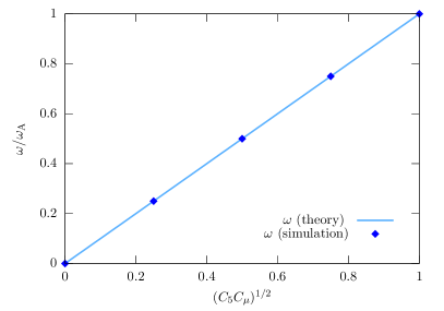
Figure 10: Dispersion relation of the chiral magnetic wave for different values of $(C_{5}C_{\mu})^{1/2}$. The simulation setups are same as in the run presented in figures 9(c)–(d), in particular $v_{\mu}=0.2$, but $(C_{5}C_{\mu})^{1/2}$ is varied between $0$ and $1$. (Colour online)

5 Conclusions

Numerical simulations are a key tool for studying the properties of high-energy plasmas, such as those of the early Universe or of proto-neutron stars. At energies $k_{\rm B}T>10\,{\rm MeV}$, the number of degrees of freedom increases by the chiral chemical potential, which is non-zero in case of an asymmetry between the number of left- and right-handed fermions. Through the additional electric current in the presence of such an asymmetry, the phenomenology of chiral MHD is even richer than that of classical MHD and numerical simulations are needed to gain a deeper understanding of the plasma and magnetic field evolution. To our knowledge, one of the first high-order parallelised codes, which has been used for chiral MHD, is the Pencil Code. A central purpose of this paper was to describe the implementation of the chiral MHD module in the Pencil Code, to discuss the relevant parameters and initial conditions in a chiral plasma, and to point out crucial differences to classical MHD. We also have presented typical applications of the chiral MHD module and discussed the obtained numerical results.

First, we have compared the initially laminar dynamo phase and the dynamo with externally driven turbulence in chiral MHD. The distinct phases in the two cases were reviewed briefly on the basis of time series and energy spectra. We have discussed the mean-field $\alpha_{\mu}^{2}$ dynamo, which can be excited in turbulence via the interaction of magnetic fluctuations due to tangling of the mean magnetic field by the fluctuating velocity and magnetic fluctuations produced by the mean chiral chemical potential. In DNS, this effect has been seen by measuring the dynamo growth rate in a stage when turbulence has been produced by the Lorentz force. Predictions of mean-field theory for the dynamo growth rate based on the $\alpha_{\mu}$ effect are in agreement with the measurements in DNS.

Second, the Pencil Code was used to check the dispersion relation of chiral MHD waves and results were compared with analytical predictions. We find agreement for the frequencies and the growth or damping rates of the chiral MHD waves: The chiral dynamo instability leads to a growth of the wave amplitude and a decrease of the frequency for chiral velocities larger than the Alfvén velocity.

Finally, we have explored the role of the ordinary chemical potential $\mu$ regarding chiral dynamos. We have demonstrated that $\mu$ can only affect the evolution of $\mu_{5}$, if the former has strong gradients. An initial sinusoidal spatial variation added to a constant $\mu_{0}$ can lead to minor variations of the velocity field in chiral-magnetically driven turbulence. Additionally, the Pencil Code was used to study chiral magnetic waves (CMWs), which occur in the presence of an imposed magnetic field and a non-vanishing coupling between $\mu$ and $\mu_{5}$. As expected, CMWs are decoupled from chiral MHD waves, at least in the linear regime of the evolution, and their frequency scales with the square root of the product of the coupling constants, i.e. $(C_{5}C_{\mu})^{1/2}$.

Appendix A Chiral MHD equations in dimensionless form

For DNS, it is convenient to move from a system formulated in physical units to a dimensionless one. This can be achieved when velocity is measured in units of the sound speed $c_{\mathrm{s}}$, length is measured in units of $\mu_{5,0}^{-1}$, where $\mu_{5,0}$ is the initial value of a uniform $\mu_{5}$, and time is measured in units of $(c_{\mathrm{s}}\mu_{5,0})^{-1}$. With the definitions ${\bm\bm{B}}=\sqrt{\overline{\rho}}\,c_{\mathrm{s}}\tilde{\bm\bm{B}}$, ${\bm\bm{U}}=c_{\mathrm{s}}\tilde{\bm\bm{U}}$, $\mu_{5}=\mu_{5,0}\,\tilde{\mu}_{5}$, $\mu=\mu_{5,0}\,\tilde{\mu}$, and $\rho=\overline{\rho}\,\tilde{\rho}$, where $\overline{\rho}$ is the volume-averaged density, the system of equations (3)–(7) can be written as

$$\frac{\upartial\tilde{\bm}{B}}{\upartial\tilde{t}} = \tilde{\bm\nabla}{\bm\times}\biggl{[}\tilde{\bm\bm{U}}{\bm\times}\tilde{\bm{B}}+{\rm Ma}_{\mu}\,\Big{(}\tilde{\mu}_{5}\tilde{\bm{B}}-\tilde{\bm\nabla}{\bm\times}{\tilde{\bm}{B}}\Big{)}\biggr{]},$$ (30)

$$\tilde{\rho}{{\mathrm{D}}\tilde{\bm}{U}\over{\mathrm{D}}\tilde{t}} = (\tilde{\bm}{\nabla}\times\tilde{\bm{B}})\times\tilde{\bm}{B}-\tilde{\bm}{\nabla}\tilde{p}+{\rm Re}_{5}^{-1}\tilde{\bm}{\nabla}{\bm\cdot}(2\tilde{\rho}\tilde{}\mbox{\boldmath${\sf S}$}{})+\tilde{\rho}\tilde{\bm}{f},$$ (31)

$$\frac{{\mathrm{D}}\tilde{\rho}}{{\mathrm{D}}\tilde{t}} = -\tilde{\rho}\,\tilde{\bm}{\nabla}\cdot\tilde{\bm}{U},$$ (32)

$$\frac{{\mathrm{D}}\tilde{\mu}_{5}}{{\mathrm{D}}\tilde{t}} = \tilde{D}_{5}\,\tilde{\Delta}\tilde{\mu}_{5}+\Lambda_{5}\,\Big{[}{\tilde{\bm}{B}}{\bm\cdot}(\tilde{\bm}{\nabla}{\bm\times}{\tilde{\bm}{B}})-\tilde{\mu}_{5}{\tilde{\bm}{B}}^{2}\Big{]}-\tilde{\Gamma}_{\mathrm{f}}\tilde{\mu}_{5}-\tilde{C}_{5}(\tilde{\bm}{B}{\bm\cdot}\tilde{\bm}{\nabla})\tilde{\mu},$$ (33)

$$\frac{{\mathrm{D}}\tilde{\mu}}{{\mathrm{D}}\tilde{t}} = \tilde{D}_{\mu}\,\tilde{\Delta}\tilde{\mu}-\tilde{C}_{\mu}(\tilde{\bm}{B}{\bm\cdot}\tilde{\bm}{\nabla})\tilde{\mu}_{5}.$$ (34)

A summary of the chiral parameters and their names in the Pencil Code can be found in Table 2. We have introduced the following dimensionless parameters.

• The chiral Mach number

  $${\rm Ma}_{\mu}={\eta\mu_{5,0}}\big{/}{c_{\mathrm{s}}}\equiv{v_{\mu}}\big{/}{c_{\mathrm{s}}},$$ (35)

  which measures the relevance of the chiral term in the induction equation (3) and determines the growth rate of the small-scale chiral dynamo instability.

• The magnetic Prandtl number

  $${\rm Pr}_{{}_{\rm M}}={\nu}/{\eta},$$ (36)

  which is equivalent to the definition in classical MHD.

• The chiral Prandtl number

  $${\rm Pr}_{{}_{5}}={\nu}\big{/}{D_{5}},$$ (37)

  which measures the ratio of viscosity and diffusion of $\mu_{5}$.

• The chemical potential Prandtl number

  $${\rm Pr}_{\mu}={\nu}\big{/}{D_{\mu}},$$ (38)

  which measures the ratio of viscosity and diffusion of $\mu$.

• The chiral nonlinearity parameter

  $$\lambda_{5}=\lambda\eta^{2}\overline{\rho},$$ (39)

  which characterises the nonlinear back reaction of the magnetic field on the chiral chemical potential $\tilde{\mu}_{5}$. The value of $\lambda_{5}$ affects the strength of the saturation magnetic field and the strength of the magnetically driven turbulence.

• The chiral flipping parameter

  $$\tilde{\Gamma}_{\mathrm{f}}={\Gamma_{\mathrm{f}}}\big{/}{\big{(}\mu_{5,0}c_{\mathrm{s}}\bigr{)}},$$ (40)

  which measures the relative importance of chiral flipping reactions.

• The coupling parameters

  $$\tilde{C}_{5}=\sqrt{\overline{\rho}}\,C_{5}$$ (41)

  and

  $$\tilde{C}_{\mu}=\sqrt{\overline{\rho}}\,C_{\mu},$$ (42)

  which measure the strength of the coupling between the evolution of $\mu$ and $\mu_{5}$, respectively.

Using the definitions above, one finds that $\tilde{D}_{5}={\rm Ma}_{\mu}\,{\rm Pr}_{{}_{\rm M}}/{\rm Pr}_{{}_{5}}$, $\tilde{D}_{\mu}={\rm Ma}_{\mu}\,{\rm Pr}_{{}_{\rm M}}/{\rm Pr}_{\mu}$, $\,\Lambda_{5}=\lambda_{5}/{\rm Ma}_{\mu}$, and ${\rm Re}_{5}=\left({\rm Ma}_{\mu}\,{\rm Pr}_{{}_{\rm M}}\right)^{-1}$ in equations (30)–(34).

Table 2: Chiral MHD parameters in the Pencil Code

Dimensionless parameter	Name in the Pencil Code
$\tilde{\mu}_{5}$	p%mu5
$\tilde{\mu}_{S}$	p%muS
$\Lambda_{5}$	lambda5
$\tilde{D}_{5}$	diffmu5
$\tilde{D}_{\mu}$	diffmuS
$\tilde{C}_{5}$	coef_mu5
$\tilde{C}_{\mu}$	coef_muS
$\tilde{\Gamma}_{\mathrm{f}}$	gammaf5

Appendix B A chiral MHD setup in the Pencil Code

An example for a minimum set up of the src/Makefile.local looks like this:

###                             -*-Makefile-*-
### Makefile for modular pencil code -- local part
### Included by ‘Makefile’
###

MPICOMM        =  nompicomm
HYDRO          =    hydro
DENSITY        =    density
MAGNETIC       =    magnetic
FORCING        =  noforcing
VISCOSITY      =    viscosity
EOS            =    eos_idealgas
SPECIAL        =    special/chiral_mhd
REAL_PRECISION =    double

Further, for running the chiral MHD module, one needs to add

   &special_init_pars
   initspecial=’const’, mu5_const=10.

to start.in and

   &special_run_pars
   diffmu5=1e-4, lambda5=1e3, cdtchiral=1.0

to run.in, where we have chosen exemplary values for the chiral parameters.

References

- Abelev et al. (2013) Abelev, B., Adam, J., Adamová, D., Adare, A.M., Aggarwal, M.M., Aglieri Rinella, G., Agocs, A.G., Agostinelli, A., Aguilar Salazar, S., Ahammed, Z. and et al., Charge separation relative to the reaction plane in Pb-Pb collisions at sNN=2.76TeV. Phys. Rev. Lett., 2013, 110, 012301.
- Alekseev et al. (1998) Alekseev, A.Y., Cheianov, V.V. and Fröhlich, J., Universality of transport properties in equilibrium, Goldstone theorem and chiral anomaly. Phys. Rev. Lett., 1998, 81, 3503–3506.
- Artsimovich and Sagdeev (1985) Artsimovich, L.A. and Sagdeev, R.Z., Plasma Physics for Physicists, 1985 (Benjamin, New York).
- Boyarsky et al. (2012) Boyarsky, A., Fröhlich, J. and Ruchayskiy, O., Self-Consistent Evolution of Magnetic Fields and Chiral Asymmetry in the Early Universe. Phys. Rev. Lett., 2012, 108, 031301.
- Boyarsky et al. (2015) Boyarsky, A., Fröhlich, J. and Ruchayskiy, O., Magnetohydrodynamics of Chiral Relativistic Fluids. Phys. Rev. D, 2015, 92, 043004.
- Brandenburg et al. (2017) Brandenburg, A., Schober, J., Rogachevskii, I., Kahniashvili, T., Boyarsky, A., Fröhlich, J., Ruchayskiy, O. and Kleeorin, N., The turbulent chiral-magnetic cascade in the early universe. ApJL, 2017, 845, L21.
- Del Zanna and Bucciantini (2018) Del Zanna, L. and Bucciantini, N., Covariant and 3 + 1 equations for dynamo-chiral general relativistic magnetohydrodynamics. MNRAS, 2018, 479, 657–666.
- Dvornikov and Semikoz (2015) Dvornikov, M. and Semikoz, V.B., Energy source for the magnetic field growth in magnetars driven by the electron-nucleon interaction. Phys. Rev. D, 2015, 92, 083007.
- Dvornikov and Semikoz (2017) Dvornikov, M. and Semikoz, V.B., Influence of the turbulent motion on the chiral magnetic effect in the early universe. Phys. Rev. D, 2017, 95, 043538.
- Dvornikov (2017) Dvornikov, M.S., Relaxation of the Chiral Chemical Potential in the Dense Matter of a Neutron Star. Russian Physics Journal, 2017, 59, 1881–1890.
- Fröhlich and Pedrini (2000) Fröhlich, J. and Pedrini, B., New applications of the chiral anomaly; in Mathematical Physics 2000, edited by A.S. Fokas, A. Grigoryan, T. Kibble and B. Zegarlinski, International Conference on Mathematical Physics 2000, Imperial college (London), 2000.
- Fukushima et al. (2008) Fukushima, K., Kharzeev, D.E. and Warringa, H.J., The Chiral Magnetic Effect. Phys. Rev., 2008, D78, 074033.
- Gailitis et al. (2000) Gailitis, A., Lielausis, O., Dement’ev, S., Platacis, E., Cifersons, A., Gerbeth, G., Gundrum, T., Stefani, F., Christen, M., Hänel, H. and Will, G., Detection of a Flow Induced Magnetic Field Eigenmode in the Riga Dynamo Facility. Phys. Rev. Lett., 2000, 84, 4365–4368.
- Gorbar et al. (2016) Gorbar, E.V., Shovkovy, I.A., Vilchinskii, S., Rudenok, I., Boyarsky, A. and Ruchayskiy, O., Anomalous Maxwell equations for inhomogeneous chiral plasma. Phys. Rev. D, 2016, 93, 105028.
- Grabowska et al. (2015) Grabowska, D., Kaplan, D.B. and Reddy, S., Role of the electron mass in damping chiral plasma instability in Supernovae and neutron stars. Phys. Rev. D, 2015, 91, 085035.
- Joyce and Shaposhnikov (1997) Joyce, M. and Shaposhnikov, M.E., Primordial magnetic fields, right electrons, and the Abelian anomaly. Phys. Rev. Lett., 1997, 79, 1193–1196.
- Kharzeev et al. (2016) Kharzeev, D.E., Liao, J., Voloshin, S.A. and Wang, G., Chiral magnetic and vortical effects in high-energy nuclear collisions—A status report. Prog. Part. Nucl. Phys., 2016, 88, 1–28.
- Kharzeev (2014) Kharzeev, D.E., The Chiral Magnetic Effect and Anomaly-Induced Transport. Prog.Part.Nucl.Phys., 2014, 75, 133–151.
- Kharzeev et al. (2013) Kharzeev, D.E., Landsteiner, K., Schmitt, A. and Yee, H.U., Strongly interacting matter in magnetic fields: an overview. Lect. Notes Phys., 2013, 871, 1–11.
- Kharzeev and Yee (2011) Kharzeev, D.E. and Yee, H.U., Chiral magnetic wave. Phys. Rev. D, 2011, 83, 085007.
- Krause and Rädler (1980) Krause, F. and Rädler, K.H., Mean-Field Magnetohydrodynamics and Dynamo Theory, 1980 (Pergamon, Oxford).
- Masada et al. (2018) Masada, Y., Kotake, K., Takiwaki, T. and Yamamoto, N., Chiral magnetohydrodynamic turbulence in core-collapse supernovae. Phys. Rev. D, 2018, 98, 083018.
- Miransky and Shovkovy (2015) Miransky, V.A. and Shovkovy, I.A., Quantum field theory in a magnetic field: From quantum chromodynamics to graphene and Dirac semimetals. Phys. Rept., 2015, 576, 1–209.
- Moffatt (1978) Moffatt, H.K., Magnetic Field Generation in Electrically Conducting Fluids, 1978 (Cambridge, England, Cambridge University Press).
- Monchaux et al. (2007) Monchaux, R., Berhanu, M., Bourgoin, M., Moulin, M., Odier, P., Pinton, J.F., Volk, R., Fauve, S., Mordant, N., Pétrélis, F., Chiffaudel, A., Daviaud, F., Dubrulle, B., Gasquet, C., Marié, L. and Ravelet, F., Generation of a Magnetic Field by Dynamo Action in a Turbulent Flow of Liquid Sodium. Phys. Rev. Lett., 2007, 98, 044502.
- Nielsen and Ninomiya (1983) Nielsen, H.B. and Ninomiya, M., The Adler-Bell-Jackiw anomaly and Weyl fermions in a crystal. Physics Lett. B, 1983, 130, 389–396.
- Rogachevskii et al. (2017) Rogachevskii, I., Ruchayskiy, O., Boyarsky, A., Fröhlich, J., Kleeorin, N., Brandenburg, A. and Schober, J., Laminar and turbulent dynamos in chiral magnetohydrodynamics-I: Theory. ApJ, 2017, 846, 153.
- Schober et al. (2018a) Schober, J., Brandenburg, A., Rogachevskii, I. and Kleeorin, N., Energetics of turbulence generated by chiral MHD dynamos. Geophys. Astrophys. Fluid Dyn., in press (arXiv:1803.06350), 2018a.
- Schober et al. (2018b) Schober, J., Rogachevskii, I., Brandenburg, A., Boyarsky, A., Fröhlich, J., Ruchayskiy, O. and Kleeorin, N., Laminar and Turbulent Dynamos in Chiral Magnetohydrodynamics. II. Simulations. ApJ, 2018b, 858, 124.
- Semikoz and Sokoloff (2005) Semikoz, V.B. and Sokoloff, D., Magnetic helicity and cosmological magnetic field. A&A, 2005, 433, L53–L56.
- Sigl and Leite (2016) Sigl, G. and Leite, N., Chiral magnetic effect in protoneutron stars and magnetic field spectral evolution. JCAP, 2016, 1, 025.
- Son and Surowka (2009) Son, D.T. and Surowka, P., Hydrodynamics with Triangle Anomalies. Phys. Rev. Lett., 2009, 103, 191601.
- Stieglitz and Müller (2001) Stieglitz, R. and Müller, U., Experimental demonstration of a homogeneous two-scale dynamo. Physics of Fluids, 2001, 13, 561–564.
- Tashiro et al. (2012) Tashiro, H., Vachaspati, T. and Vilenkin, A., Chiral effects and cosmic magnetic fields. Phys. Rev. D, 2012, 86, 105033.
- Vilenkin (1980) Vilenkin, A., Equilibrium parity violating current in a magnetic field. Phys. Rev. D, 1980, 22, 3080–3084.
- Wang (2013) Wang, G., Search for Chiral Magnetic Effects in High-Energy Nuclear Collisions. Nuclear Physics A, 2013, 904-905, 248c – 255c The Quark Matter 2012.
- Yamamoto (2016) Yamamoto, N., Scaling laws in chiral hydrodynamic turbulence. Phys. Rev. D., 2016, 93, 125016.
- Zeldovich et al. (1983) Zeldovich, Y.B., Ruzmaikin, A.A. and Sokoloff, D.D., Magnetic Fields in Astrophysics, 1983 (Gordon and Breach, New York).