Beyond $\Lambda$CDM with Low and High Redshift Data: Implications for Dark Energy

Abstract

Assuming that the Universe at higher redshifts ($z\sim 4$ and beyond) is consistent with $\Lambda$CDM model as constrained by the Planck measurements, we reanalyze the low redshift cosmological data to reconstruct the Hubble parameter as a function of redshift. This enables us to address the $H_{0}$ and other tensions between low $z$ observations and high $z$ Planck measurement from CMB. From the reconstructed $H(z)$, we compute the energy density for the “dark energy” sector of the Universe as a function of redshift without assuming a specific model for dark energy. We find that the dark energy density has a minimum for certain redshift range and that the value of dark energy at this minimum ${\rho}_{{}_{\text{DE}}}^{\text{min}}$ is negative. This behavior can most simply be described by a negative cosmological constant plus an evolving dark energy component. We discuss possible theoretical and observational implications of such a scenario.

Keywords: Dark energy, Low redshift data, CMB, H0 tension.

1 Introduction

Thanks to various sets of cosmological data, we can now talk about “the standard model of cosmology”, the $\Lambda$CDM Universe [1, 2]. It provides the simplest paradigm that fits remarkably well to most of the current cosmological observations. As the precision of the low redshift data increases, there are however emerging tensions in $\Lambda$CDM model which is otherwise consistent with high redshift CMB observations by Planck. The major tension is between the model independent measurement of $H_{0}$ parameter ($\sim 73\leavevmode\nobreak\ \text{km/s/Mpc}$) by SH0ES collaboration [3, 4, 5] and that by Planck assuming $\Lambda$CDM model [1, 2, 6, 7]. The latest Planck-2018 data shows, $H_{0}=67.8\pm 0.9\leavevmode\nobreak\ \text{km/s/Mpc}$ [6] and this is at tension over $3.5\sigma$ with the SH0ES measurement which is $H_{0}=73.52\pm 1.62\leavevmode\nobreak\ \text{km/s/Mpc}$. A similar mild inconsistency in $H_{0}$ for $\Lambda$CDM model is also observed by Strong Lensing experiments like H0LiCow using time delay measurements [8] which measured $H_{0}=71.9^{+2.4}_{-3.0}\leavevmode\nobreak\ \text{km/s/Mpc}$ for $\Lambda$CDM Universe. Moreover the BOSS survey for baryon acoustic oscillations measurements using Lyman-$\alpha$ forest [9] has also measured the expansion rate of the Universe at $z=2.34$. This measured expansion rate of the Universe at $z=2.34$ is also at tension over $2\sigma$ with Planck result for $\Lambda$CDM [10]. The important consequences of these tensions are the prediction of the dark energy density evolution with time and more importantly for us, the possibility of having negative dark energy density at higher redshifts as discussed by [9, 10, 19]. Similar conclusion has also been obtained recently by [20] using a dark energy model independent approach. In their study, Wang et al. attributed the evolution of dark energy density as well as its negative values at high redshifts to non-minimally coupled scalar field theory like Brans-Dicke theory. Interestingly in all these studies, the dark energy density is not only negative at higher redshifts but it is unbounded from below. This poses a serious problem as in a spatially flat universe, with such a negative dark energy density, the matter energy density parameter will be more than one and grow quickly without any upper bound at higher redshifts. This will have catastrophic effect on the structure formation scenario.This surely needs to be resolved.

In this work, we revisit the process of constraining the dark energy behavior using cosmological observations to find the likely sources of tensions between low and high redshifts cosmological observations. For this, we should be careful that although Planck constrains the high redshift Universe using CMB with unprecedented accuracy, it may not be sensitive enough to any new physics beyond $\Lambda$CDM at low redshifts. Fitting the entire background evolution of the Universe from $z\sim 1100$ till $z=0$ using $\Lambda$CDM in which the dark energy density is a redshift independent quantity, can be the source of aforementioned tensions.

Therefore we reanalyze the low-redshift data involving background cosmology assuming that for a certain higher redshift $z=z_{\text{match}}$ and beyond, one recovers the background evolution as constrained by Planck-2018 for $\Lambda$CDM Universe. For this, we assume that $z_{\text{match}}$ has to be larger than $z\sim 2.4$, as around this redshift, we have the constraint on expansion rate of Universe from BOSS survey using Lyman-$\alpha$ forest. This takes care of any new physics for dark energy evolution (beyond $\Lambda$CDM Universe) that is predicted by low-redshift observations for $z<z_{\text{match}}$ including the SH0ES measurement for $H_{0}$. With these assumptions, we study the dark energy behaviour which is consistent with the low-redshift data for $z\leq z_{match}$ while smoothly matching the Planck-constrained $H(z)$ behaviour for $\Lambda$CDM model for $z>z_{match}$. In this process, we do not assume any particular dark energy model. We directly reconstruct the Hubble parameter $H(z)$ as a function of redshift using cosmographic approach. Subsequently, we reconstruct the dark energy density evolution in a “dark energy relaxed XCDM framework,” in which we do not assume any specific dark energy model, while still assume the Universe is spatially flat and contains pressure-less matter (including baryons and dark matter) plus another unknown component. This extra unknown component can be due to dark energy or it may arise as an effective dark energy component due to any sort of modification of gravity at large cosmological scales. We also ignore the contribution from radiation energy density as it is negligible compared to matter or dark energy at late times.

Our dark energy model-independent analysis within the above set of working assumptions and framework reveals that ${\rho}_{{}_{\text{DE}}}(z)$ has two specific features: it has a minimum and a phantom crossing at $z=z_{\text{min}}$. Moreover, the value of ${\rho}_{{}_{\text{DE}}}$ at $z=z_{\text{min}}$ is negative. The simplest explanation for ${\rho}_{{}_{\text{DE}}}^{\text{min}}<0$, is the existence of a negative Cosmological Constant.

2 Data sets and their analysis

There are different approaches to constrain the behavior of dark energy without assuming any particular dark energy model. Here we take the cosmographic approach that directly constrains different kinematical quantities related to the background evolution. The Taylor expansion of $H(z)$ for this purpose does not work for $z>1$ and hence we use the Pade Approximation that improves the convergence at higher redshifts [25, 26, 27, 28, 29, 30].

For our purpose we model the Hubble parameter $H(z)$ using Pade approximation $P_{2,2}$:

$$H(z)=H_{0}\frac{1+P_{1}z+P_{2}z^{2}}{1+Q_{1}z+Q_{2}z^{2}}.$$ (1)

All the constant parameters $P_{1},P_{2},Q_{1},Q_{2}$ appearing in the above expression, can be written in terms of the kinematic quantities like, $q,j,s,l$ (deceleration, jerk, snap, and lerk) (see [31] for details). Note that for $\Lambda$CDM model, the jerk parameter $j=1$ for all redshifts and any deviation from $j=1$, confirms a non-$\Lambda$CDM behavior.

In the following two subsections we reconstruct $H(z)$ in two cases to highlight the effects of inclusion of constraint on background expansion at high redshifts from Planck measurements of CMB anisotropy: In section 2.1 we only consider the low redshift data samples mentioned below using Pade approximant. In section 2.2 we reanalyze the low redshift data requiring $H(z)$ passes through three data points at $z_{\text{match}},z_{\text{match}}\pm 1$. The former may then be used to compare with results of [17, 20]. This analysis may be viewed as a check for the Pade parametrization used.

2.1 Low redshift data only

To constrain the background cosmology, we use the following set of low-redshift observational data:

• BAO measurements from different surveys including eBoss quasar clustering and Lyman-$\alpha$ forest samples (see [32] and references therein);

• latest Pantheon data for SNIa [4, 33];

• the OHD data for Hubble parameter at different redshifts [34];

• strong lensing time-delay measurements by H0LiCOW experiment [8];

• angular diameter distances measured using water megamasers under the Megamaser Cosmology Project [32, 35, 36, 37];

• finally the measurement of $H_{0}$ by [3][R16].

For details about all the data used in this analysis, please refer to [31]. The independent parameters for the data analysis are $H_{0},q_{0},j_{0},s_{0}$, $l_{0}$ and $r_{d}$, the sound horizon at drag epoch. Here the subscript $``0"$ means the value at present ($z=0$).

The reconstructed $H(z)$ is shown in Fig.1 (Left-Top plot). Note that the high uncertainty beyond $z\sim 2.4$ is due to unavailability of low redshift data beyond $z\sim 2.4$. As one can see (the Right-Top plot), the reconstructed $H(z)$ from low-redshift observations is at large tension with the same, reconstructed from Planck-2018 data. Also at low redshifts ($z\leq 2$), there is oscillations in $H(z)$ behaviour around the best fit $H(z)$ behaviour for $\Lambda$CDM as measured by Planck-2018. Such oscillation in $H(z)$ has already been reported in [20] through a model independent study. In this work, we obtain exactly the same behaviour in a completely different approach using Pade approximation for cosmography.

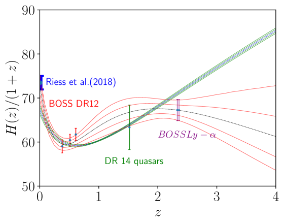
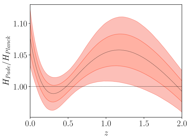
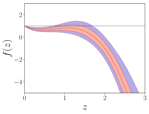
Figure 1: Low data redshift analysis without inclusion of high redshift CMB data from Planck. Left-Top: Reconstructed Hubble parameter $H(z)$ from various low-redshift data sets. The black dashed line is for best fit values whereas the inner and outer lines denote $1\sigma$ and $2\sigma$ contours. The thin shaded region is reconstructed $H(z)$ behaviour from Planck-2018 measurements. Right-Top: Comparison of our reconstructed $H(z)$ using Pade approximant and the best fit $H(z)$ for $\Lambda$CDM by Planck-2018. Bottom: Reconstructed dark energy density as a function of redshift. The horizontal line $f(z)=1$ is for $\Lambda$CDM.

Once we constrain the $H(z)$ behaviour using available low-redshift data, we can further constrain the redshift evolution of any exotic component which one needs to add to the matter contribution. This extra component (we denote it as ${\rho}_{{}_{\text{DE}}}$) can be due to dark energy or due to any modification of gravity on large cosmological scales that gives rise to some effective dark energy component. Following [20], we write:

$$3H^{2}(z)=\rho_{m}+{\rho}_{{}_{\text{DE}}}=\rho_{m0}(1+z)^{3}+\rho_{{}_{\text{DE}0}}f(z).$$ (2)

Here we set $8\pi G=1$ and superscript “0" indicates values at present $z=0$ and subscript “DE” stands for any dark component (either actual or effective) that yields late time acceleration. The $f(z)$ (a dimensionless quantity) specifies the allowed redshift evolution of ${\rho}_{{}_{\text{DE}}}$. Assuming a flat Universe, $\Omega_{m}+\Omega_{\text{DE}}=1$, equation (2) can be rewritten as

$$\frac{H^{2}}{H_{0}^{2}}=\Omega^{(0)}_{m}(1+z)^{3}+\Omega^{(0)}_{\text{DE}}f(z)=\Omega^{(0)}_{m}(1+z)^{3}+(1-\Omega^{(0)}_{m})f(z).$$ (3)

With this, one can constrain the redshift evolution for ${\rho}_{{}_{\text{DE}}}(z)$ using the behaviour for $H(z)$ shown in Fig.1. For this, one needs to assume the value of $\Omega^{(0)}_{m}$ and for our purpose, we assume $\Omega^{(0)}_{m}=0.315$ which is best fit value for Planck-2018 for $\Lambda$CDM and this value is not very sensitive to dark energy behaviour. Using this, one can now reconstruct the $f(z)$ behaviour from low-redshift observation which is shown in Fig. 1 (Bottom plot). As one can see, the $f(z)$ clearly shows oscillations around the $f(z)=1$ $\Lambda$CDM behaviour for low redshifts. This confirms the phantom-non phantom crossing. Also for larger redshifts, $f(z)<0$ and is also unbounded from below. These behaviours of $f(z)$ are in complete agreement with the results obtained by [20], confirming our methodology of using Pade approximations.

2.2 Low redshift data plus inclusion of CMB Planck data points for H(z)

Once we confirm the results obtained by [20] as well as other authors [10, 9, 19] with different approach, our next goal is to solve the problem of ${\rho}_{{}_{\text{DE}}}$ being unbounded from below for negative values for larger redshifts. To address this problem, we assume that $H(z)$ as constrained by the low redshift data, should also fit $H(z)$ as measured by Planck for $\Lambda$CDM at some higher redshift $z=z_{\text{match}}$ and beyond. This assumption is well justified noting that the difference between our XCDM model and $\Lambda$CDM is in their dark energy sector and that the dark energy effects becomes relevant to the evolution of the Universe only at lower redshifts. Also as discussed in the Introduction, to take into account any new physics in the dark energy sector that may arise due to the BAO observations at $z=2.4$ using Lyman-$\alpha$ forest, $z_{\text{match}}\gtrsim 4$ should be a reasonable choice. Of course, as we will comment in the discussion part, in a full and complete analysis, $z_{\text{match}}$ should also come out from the analysis itself. Here we only intend to present a “proof of concept” analysis.

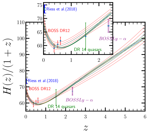
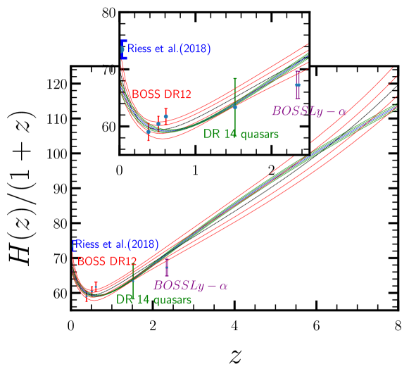
Figure 2: Reconstructed Hubble parameter $H(z)$ behavior employing both low redshift and CMB Planck data sets, see the text for details. The left one is based on Planck $H(z)$ data at $z=4,5,6$ and right one is for $z=6,7,8$. The dashed line is for mean and inner and outer regions are for $68\%$ and $95\%$ confidence regions. The thin shaded region is reconstructed $H(z)$ behaviour from Planck-2018 measurements.

To this end, we generate $H(z)$ data points for higher redshifts using Planck sample chains and use those data for the fitting. We use two sets of data for this purpose: in one case we generate data for $H(z)$ using Planck $\Lambda$CDM chains for redshifts $z=4,5,6$ [hereafter we refer this case as PL1] assuming $z_{match}\sim 4$ and in another case we do the same for $z=6,7,8$ [hereafter we refer his case PL2] assuming $z_{match}\sim 6$. In both cases, we use sample chains for Planck+WP+highL+lensing-2015 for baseline $\Lambda$CDM model [42].

The reconstructed Hubble parameter, as a function of $z$, is shown in Fig.2. As one can see, the reconstructed $H(z)$ fits the $H_{0}$ data from R16 as well as $H(z)$ points as measured by Planck-2015 for $\Lambda$CDM model [1] at higher redshifts. The constraints on deceleration and jerk parameters at $z=0$ are: ($q_{0}=-0.83^{+0.10}_{-0.10},j_{0}=3.93^{+0.53}_{-0.53}$) and ($q_{0}=-0.94^{+0.11}_{-0.10},j_{0}=4.31^{+0.51}_{-0.53}$) for PL1 and PL2 respectively. Clearly $j_{0}=1$ is ruled out with high confidence level confirming the inconsistency with $\Lambda$CDM model at present. This is consistent with previous results by [17] and [20].

Once we constrain the $H(z)$ using above data points, we again reconstruct the dark energy behavior through $f_{{}_{\text{DE}}}(z)$ as described equations (4) and (5). Here instead of choosing a particular value for $\Omega_{m0}$, we choose two different values, $0.3$ and $0.32$ respectively to see effect of $\Omega_{m0}$ on reconstructed $f(z)$. The result is shown in Fig 3.

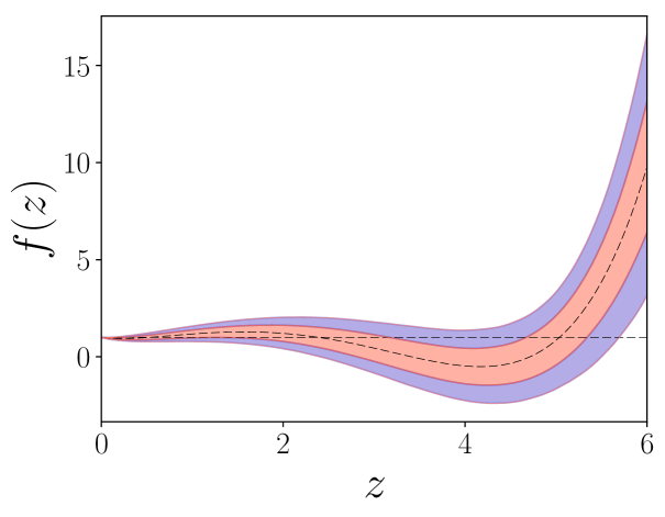
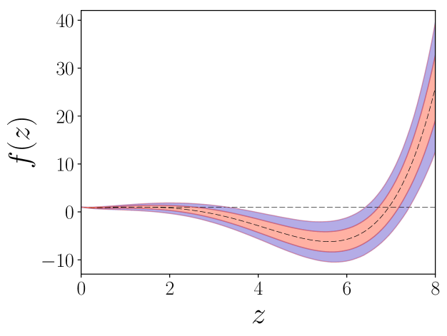
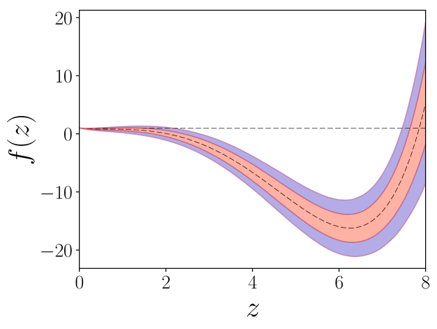
Figure 3: Reconstructed $f(z)$. The top ones for PL1 whereas the bottom ones are PL2. In each case, left ones are for $\Omega^{(0)}_{m}=0.3$ and right ones are for $\Omega^{(0)}_{m}=0.32$. The different regions and lines are same as in Fig.2.

As one can see, $f(z)$ exhibits two generic features: (1) the overall shape for $f(z)$ is the same for different choices of $\Omega^{(0)}_{m}$ as well as the redshift range where we generate $H(z)$ data using Planck chains for $\Lambda$CDM. It has always a minimum at some $z=z_{\text{min}}$, and generically $f(z)<0$ at this minimum; (2) $z_{\text{min}}$ and $f_{\text{min}}=f(z_{\text{min}})$ depend on the value of $\Omega^{(0)}_{m}$ and the range of redshifts where one takes the $H(z)$ data from Planck. For $\Omega^{(0)}_{m}>0.29$, there is always a negative minimum for $f(z)$, and for $H(z)$ data from the Planck at higher redshift range, the negative minimum for $f(z)$ exists with a greater confidence level. The presence of this negative minimum in ${\rho}_{{}_{\text{DE}}}(z)$ does not affect the background evolution. This can be seen from Fig.2 that there is no pathological behavior in $H(z)$ which is perfectly consistent with a late time accelerating Universe.

3 Generic Results

$f(z)$ is essentially showing “time dependence” of the dark energy density ${\rho}_{{}_{\text{DE}}}(z)$, therefore the time derivative of ${\rho}_{{}_{\text{DE}}}$ vanishes at $z_{\text{min}}$:

$$\dot{\rho}_{{}_{\text{D}E}}(z)|_{z=z_{\text{min}}}=0\ \ \ \Longrightarrow\hskip 5.69054pt({\rho}_{{}_{\text{DE}}}+{P}_{{}_{\text{DE}}})_{z=z_{\text{min}}}=0.$$

That is, at the minimum, the ${\rho}_{{}_{\text{DE}}}$ behaves like a cosmological constant. Moreover, this minimum value being negative, can be simply modeled through a negative cosmological constant with $\Lambda=3H_{0}^{2}(1-\Omega^{(0)}_{m})f_{\text{min}}$. The most significant outcome of our analysis is that the low redshift data together with Planck constraint on $H(z)$ for $\Lambda$CDM at higher redshifts allows for a negative cosmological constant.

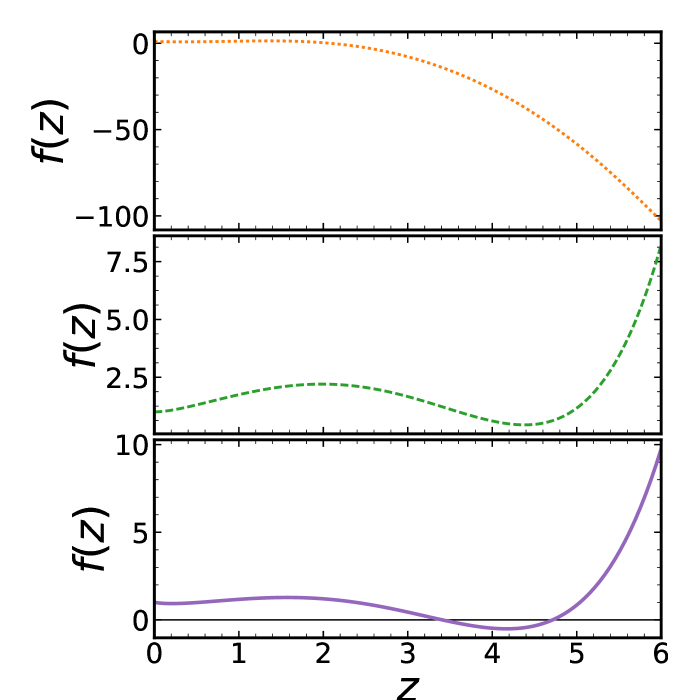
Figure 4: Reconstructed $f(z)$. The mean $f(z)$ is plotted from the MCMC chains. The top one is without $H_{0}$ data as well as without taking Planck points for $H(z)$ for higher redshifts. The middle one is without $H_{0}$ data but taking Planck points for $H(z)$ for higher redshifts. The bottom one is taking both the $H_{0}$ data and Planck Points for $H(z)$ for higher redshifts. The rest of the low redshift data as mentioned in the text are taken in all plots. Planck points for $H(z)$ are for PL1 and $\Omega^{(0)}_{m}=0.3$ is assumed.

As discussed in the Introduction, the negative ${\rho}_{{}_{\text{DE}}}$ without any minimum for higher redshifts has already been confirmed by [20] using low redshift data in a model independent way. The new feature in our analysis is the inclusion of the Planck’s constraints on $H(z)$ for higher redshifts. This yields to a lower negative bound on $\rho_{DE}$ which can be associated with a negative Cosmological Constant. To show these dependencies, in Fig. 4 we plot the mean $f(z)$ behavior from our reconstruction for a specific case. The topmost behavior is without including $H_{0}$ data from R16 and also without including $H(z)$ data generated using Planck $\Lambda$CDM chains. The $f(z)$ clearly goes to negative values at higher redshifts as confirmed by [20], and this is mainly due to Lyman-$\alpha$ measurement of BAO at $z\sim 2.4$ as pointed out in [20], see also [9, 19]. Next we add the $H(z)$ data from Planck at higher redshift and this results a minimum in $f(z)$ which is positive. Finally, as we add the $H_{0}$ data from R16, the minimum shifts to a negative value. The inclusion of $H_{0}$ data from R16 enforces present Hubble parameter to be larger which can be compensated by lowering (even negative) dark energy density in the intermediate redshifts. Hence the Lyman-$\alpha$ data at $z\sim 2.4$, the $H_{0}$ data from R16 as well as the constraints from Planck on $H(z)$ at higher redshifts, all together play the crucial role for having a negative minimum for ${\rho}_{{}_{\text{DE}}}$ which may be modelled by a negative Cosmological Constant.

The above conclusion can also be seen in this following way. Several previous analysis with low redshift data [20], [9, 19] including our current analysis indicate that $f(z)$ becomes negative at some $z>1$. At the same time, $H(z)$ should also go to matter domination at higher redshift. Then the only option for $f(z)$ is that it start with some positive value at $z=0$, starts decreasing for $z>0$, becomes negative at some point, attains a minimum with a negative value and then increases to $0$ for higher $z$, before matching to the Planck data at around $z_{\text{match}}.$

Moreover, for $z>z_{\text{min}}$, the $\rho_{{}_{\text{DE}}}$ decreases with time, whereas for $z<z_{\text{min}}$, it increases with time, confirming the phantom crossing at $z=z_{\text{min}}$. The phantom region in this case cannot be mimicked by a minimally coupled scalar field rolling uphill the potential as discussed in [43, 44]. This is because for a minimally coupled scalar field $\phi$, at $\rho_{{}_{\text{DE}}}^{\text{min}}$, $\frac{d{\phi}}{dt}=0$, which does not allow $\phi$ to roll uphill the potential.

4 Discussion and Outlook

Based on two requirements that $H_{0}$-tension is ameliorated (in favor of [3]) and $\Lambda$CDM is still the best fit for Planck data at higher redshifts, we reanalyzed the low redshift data. If we consider just the low-redshift data, as we did in section 2.1, we get $H_{0}=72.56\pm 1.55$, which is perfectly consistent with [3]. Adding the $H(z)$ data for higher redshift from Planck chains for $\Lambda$CDM as we did in section 2.2, we get the following results: For $z_{\text{match}}=4$, $H_{0}=68.7\pm 1.3$, which is $2.3\sigma$ tension with [5]. For $z_{\text{match}}=6$, $H_{0}=70.0\pm 1.4$ which is at $1.65\sigma$ tension with [5] and is at less than $2\sigma$ tension with [45]. The details of these analysis will appear in an upcoming paper. So the take away is: (1) adding the Planck constraint on background evolution at higher redshifts, the $H_{0}$ shifts towards lower values compared to only low-redshift analysis and (2) adding the data point from $H(z)$ reconstructed by Planck chains, prefers higher $z_{\text{match}}$. As we already pointed out with higher $z_{\text{match}}$ the likelihood of having negative minimum in $f(z)$ is greater. As we mention below, the exact value of $z_{\text{match}}$ should be obtained with a thorough analysis including low redshift and full CMB likelihood.

We reconstructed the $H(z)$ behavior for $z\lesssim 8$ region and subsequently the ${\rho}_{{}_{\text{DE}}}(z)$ behavior. We stated and discussed three generic results of our analysis in the previous sections. It is important to highlight the differences of our work from some recent works along this line. In the work by [17], the equation of state parameter for the dark energy was reconstructed with the assumption of ${\rho}_{{}_{\text{DE}}}>0$, and also no interaction between matter and the dark energy, therefore, setting aside a very large class of dark energy models including modified gravity models. In a subsequent paper by [20], ${\rho}_{{}_{\text{DE}}}$ was reconstructed directly, and it was found to be unbounded from below at higher redshifts. Almost similar inference was drawn in [19]. In our analysis, we directly reconstruct the $H(z)$ from low redshift data using Pade approximation and get the similar result. Our analysis reproduces the result of [20] that ${\rho}_{{}_{\text{DE}}}<0$ at higher redshift. The fact that two different reconstructions yield similar results, supports the validity of our $H(z)$ reconstruction process which is based on Pade parametrization.

Subsequently we incorporated Planck constraint on background universe, directly through $H(z)$ as measured by Planck for $\Lambda$CDM at intermediate redshifts. This makes sure that our reconstructed $H(z)$ from low redshift data is consistent with Planck measured $H(z)$ for $\Lambda$CDM at intermediate redshifts. This results in a minimum for ${\rho}_{{}_{\text{DE}}}$ and this minimum is negative. The notable features of our approach for low-redshift data analysis are direct $H(z)$ reconstruction (using Pade approximant/parametrization) and imposing Planck constraint on $H(z)$ at intermediate redshifts.

Below, we add some further comments and things to be worked out and studied in future:

• Vetting the working assumptions and robustness of our results:

  This is probably the first study where we assume two different $H(z)$ behavior at low and high redshifts and match them around some $z=z_{\text{match}}$, for which we chose some reasonable values. To justify this working assumption, we have tested different $z_{\text{match}}$ and overall behavior of our results remain the same. This is also shown in Fig.3, where we plot $f(z)$ for two different choices of redshift range to generate $H(z)$ data from Planck $\Lambda$CDM model. Of course, to get an actual estimate of $z_{\text{match}}$, one needs to do a full combined analysis using all the low redshift data together with Planck Likelihood assuming that for $z\leq z_{\text{match}}$, $H(z)$ is given by (1) and for $z>z_{\text{match}}$, $H(z)$ is given by $\Lambda$CDM model and get a estimate of $z_{\text{match}}$. This is beyond the scope of present study and will be reported in a separate publication.

  Our other working assumption was the use of Pade Approximation. Pade approximation has been extensively used earlier for low-redshift reconstruction purposes, more detailed references can be found in [25] and more recent usage of Pade parametrization in [10, 46, 26, 27, 28, 29] . Probably the first work on reconstruction of quintessence potential using Type-Ia Supernova data used the rational function like Pade Approximation to model the Luminosity Distance [25]. In our case, we use the same for the Hubble Parameter with larger set of observational data. We emphasis that use of Pade Approximation to reconstruct of Hubble parameter does not bias the final result. The result that dark energy density can be negative at higher redshifts (primarily due to $H_{0}$ measurement by Riess et al and the Lyman-$\alpha$ measurement of BAO at $z\sim 2.4$) has been also confirmed by several earlier works. It is, however, useful to reanalyze the data using other parametrizations and verify that the final features and results do not depend on the parametrization used in any crucial way.
  

• Consistency with Planck’s measurement of the CMB anisotropy:

  

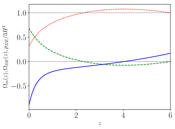
  Figure 5: The dotted red line is for $\Omega_{\text{m}}(z)$, the dashed green line is for $\Omega_{{}_{\text{DE}}}(z)$ and the solid blue line is for ${P}_{{}_{\text{DE}}}/(3H^{2})$. This is for Planck H(z) data at $z=4,5,6$ and $\Omega^{(0)}_{m}=0.32$.

  The simplest dark energy model we can suggest based on our results is a negative Cosmological Constant and a phantom crossing for the rest of the dark energy. To show that such a model is consistent with CMB temperature anisotropy as measured by Planck, we calculate $C_{l}^{TT}$ for CMB anisotropy spectra assuming that till $z\leq 6$, $H(z)$ is given by best fit of our reconstructed $H(z)$ and for $z>6$, it is given by Planck best fit $\Lambda$CDM model [1, 2] . Note that at $z=6$, $\Lambda$CDM model is well within matter dominated era. In Fig. 5, we show the behaviours of density parameters for matter and dark energy. As one can see, around $z=6$, $\Omega_{m}=1$ and $\Omega_{\text{DE}}=0$, allowing us to match our reconstructed $H(z)$ with a matter dominated era.

  Using this $H(z)$, we use CLASS code [47] to compute the $C_{l}^{TT}$ and compare with Planck data as well as Planck best fit $\Lambda$CDM model. The result is shown in Fig.6. As expected and one can see, $C_{l}^{TT}$ in our model is a good fit to Planck’s measurement.
  

• Effects on Structure Formation:

  The existence of this small negative $\Lambda$ can have interesting effect on growth of structures. As one can see in Fig. 5, $\Omega_{m}$ is slightly greater than $1$ for a certain redshift range depending on where we match the $H(z)$ with Planck’s $\Lambda$CDM model. This will give enhancement in growth of structures at higher redshifts and the nonlinear regime may start earlier than in $\Lambda$CDM model. This may result in the presence of more massive galaxies at higher redshifts compared to $\Lambda$CDM model, effects on reionization process as well as on lensing. All these are potential observable signatures for our model that can be tested by present and next generation galaxy surveys and CMB experiments.
  

• Modeling the ${\rho}_{{}_{\text{DE}}}(z)$:

  Within our data analysis framework, we have a clear indication that dark energy sector cannot be described by only a cosmological constant. Moreover, as discussed, ${\rho}_{{}_{\text{DE}}},{P}_{{}_{\text{DE}}}$ cannot be obtained from a minimally coupled scalar field (with any potential); that is, quintessence models do not lead to our ${\rho}_{{}_{\text{DE}}}(z)$. Given that ${\rho}_{{}_{\text{DE}}}$ takes negative values for a range of $z$, the simplest model is to assume presence of a negative cosmological constant with its value $\Lambda=\rho_{\text{min}}$ and then try to model $\rho={\rho}_{{}_{\text{DE}}}-\rho_{\text{min}}$ within a non-minimally coupled scalar theory with a positive definite potential. This latter should be such that it provides crossing to phantom region $({\rho}_{{}_{\text{DE}}}+{P}_{{}_{\text{DE}}}<0)$ for $z<z_{\text{min}}$. Such models can be constructed, e.g. within Brans-Dicke theory [20]. Seeking and exploring such models is postponed to future works.
  

• Theoretical implications of our dark energy model:

  A positive cosmological constant which is assumed to drive the current accelerated expansion of the Universe is a theoretical challenge: Getting a vacuum solution with a positive cosmological constant within moduli-fixed consistent and stable string theory compactifications has been a daunting task [48, 49, 50, 51]. Moreover, formulating quantum field theory on the background of a de Sitter space has its own challenges, from the choice of the vacuum state to non-existence of a well-defined S-matrix (on global de Sitter space) [52, 53]. Our findings here, lifts all those questions by simply removing the need for a positive cosmological constant.

  

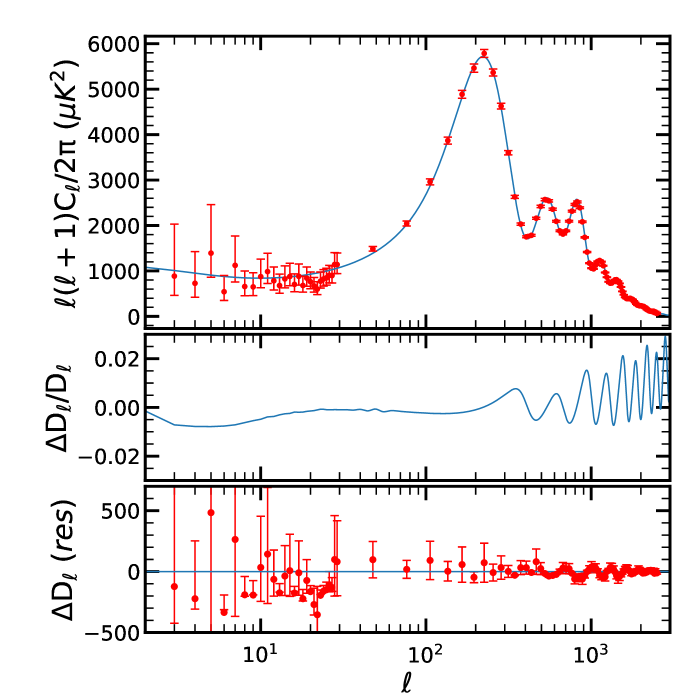
  Figure 6: CMB TT spectra. Top one: for model considered in this work (see text) together with Planck data and error bars for TT spectra. Middle one: the difference in TT spectra for our model and Planck best fit $\Lambda$CDM model. Bottom one: The residual for our model with the Planck data.

  On the other hand, a negative cosmological constant is a theoretical sweet spot: it provides an anti-de Sitter (AdS) background, which is very much welcome due to AdS/CFT duality [54], providing a “dual” framework for cosmology. In addition, string theory clearly prefers AdS background to de Sitter, consistent AdS backgrounds are ubiquitous in string theory settings [55]. Interestingly, it has been argued that accelerated expansion of the Universe may be possible with a negative cosmological constant [56].

  Finally, we comment on the recently proposed “swampland” conjecture [57] which favors quintessence models over $\Lambda$CDM. Our results here are in clear tension with the swampland conjecture. Similar statement has also been made in [58].
  

• Our results and anthropic reasoning.

  In mid 1980’s and long before observational establishment of late-time cosmic acceleration, based on structure formation constraints which is necessary to yield existence of life (as it is usually perceived) it was argued that the value of cosmological constant, if positive, should not be much bigger than $H_{0}^{2}$ [59]. A negative value of the cosmological constant, too, is bounded by similar anthropic reasoning [60]. Interestingly, the negative cosmological constant in our model which is within $1\%$ of the current total energy density of the Universe is certainly consistent with these bounds.

We emphasize that we ascribe the tension between the inferred value of $H_{0}$ between the local measurements and the Planck data fully on the dynamics of dark energy. Given this is the true case for this tension, what we find is that a negative value of the cosmological constant is still allowed by the data. To summarise, we discuss the prospects of solving the tension between low and high redshift cosmological observations in the presence of a small negative cosmological constant. This is probably the first time, that there are observational suggestions for presence of a negative cosmological constant. Its presence predicts definite observational signatures in large scale structure formation in the Universe and can be tested with present and future experiments.

Note added: As we were updating and revising our paper, the paper [45] appeared which has now a new measured value for $H_{0}$ which is $74.03\pm 1.42$ km/s/Mpc. This is now in tension with Planck-2018 measurement for $H_{0}$ at $4.4\sigma$. For our case with PL2 ($z_{match}=6$), the value for $H_{0}$ is $70^{+1.45}_{-1.50}$ Km/s/Mpc. The deviation of this value with [45] is $1.98\sigma$ which is at less than $2\sigma$ tension. See also [61] for more discussions and analysis.

References

- [1] Planck Collaboration, P. A. R. Ade et al., “Planck 2015 results. XIII. Cosmological parameters,” Astron. Astrophys. 594 (2016) A13, 1502.01589.
- [2] Planck Collaboration, P. A. R. Ade et al., “Planck 2015 results. XIV. Dark energy and modified gravity,” Astron. Astrophys. 594 (2016) A14, 1502.01590.
- [3] A. G. Riess et al., “A 2.4% Determination of the Local Value of the Hubble Constant,” Astrophys. J. 826 (2016), no. 1, 56, 1604.01424.
- [4] A. G. Riess et al., “Type Ia Supernova Distances at Redshift >1.5 from the Hubble Space Telescope Multi-cycle Treasury Programs: The Early Expansion Rate,” Astrophys. J. 853 (2018), no. 2, 126, 1710.00844.
- [5] A. G. Riess et al., “Milky Way Cepheid Standards for Measuring Cosmic Distances and Application to Gaia DR2: Implications for the Hubble Constant,” Astrophys. J. 861 (2018), no. 2, 126, 1804.10655.
- [6] Planck Collaboration, Y. Akrami and others (Planck 2018 Collaboration), “Planck 2018 results. I. Overview and the cosmological legacy of Planck,” 1807.06205.
- [7] Planck Collaboration, N. Aghanim and others (Planck 2018 Collaboration), “Planck 2018 results. VI. Cosmological parameters,” 1807.06209.
- [8] V. Bonvin et al., “H0LiCOW - V. New COSMOGRAIL time delays of HE 0435-1223: H0 to 3.8 per cent precision from strong lensing in a flat LCDM model,” Mon. Not. Roy. Astron. Soc. 465 (2017), no. 4, 4914–4930, 1607.01790.
- [9] BOSS Collaboration, T. Delubac et al., “Baryon acoustic oscillations in the Ly-alpha forest of BOSS DR11 quasars,” Astron. Astrophys. 574 (2015) A59, 1404.1801.
- [10] V. Sahni, A. Shafieloo, and A. A. Starobinsky, “Model independent evidence for dark energy evolution from Baryon Acoustic Oscillations,” Astrophys. J. 793 (2014), no. 2, L40, 1406.2209.
- [11] J. Sola Peracaula, A. Gomez-Valent, and J. d. C. Perez, “Signs of Dynamical Dark Energy in Current Observations,” Phys. Dark Univ. 25 (2019) 100311, 1811.03505.
- [12] J. Solà Peracaula, J. de Cruz Pérez, and A. Gómez-Valent, “Dynamical dark energy vs. = const in light of observations,” EPL 121 (2018), no. 3, 39001, 1606.00450.
- [13] J. Ryan, S. Doshi, and B. Ratra, “Constraints on dark energy dynamics and spatial curvature from Hubble parameter and baryon acoustic oscillation data,” Mon. Not. Roy. Astron. Soc. 480 (2018), no. 1, 759–767, 1805.06408.
- [14] J. Ooba, B. Ratra, and N. Sugiyama, “Planck 2015 constraints on spatially-flat dynamical dark energy models,” 1802.05571.
- [15] E. Di Valentino, A. Melchiorri, E. V. Linder, and J. Silk, “Constraining Dark Energy Dynamics in Extended Parameter Space,” Phys. Rev. D96 (2017), no. 2, 023523, 1704.00762.
- [16] A. Bonilla Rivera and J. G. Farieta, “Exploring the Dark Universe: constraints on dynamical Dark Energy models from CMB, BAO and growth rate measurements,” Int. J. Mod. Phys. D28 (2019), no. 09, 1950118, 1605.01984.
- [17] G.-B. Zhao et al., “Dynamical dark energy in light of the latest observations,” Nat. Astron. 1 (2017), no. 9, 627–632, 1701.08165.
- [18] Y. Zhang, H. Zhang, D. Wang, Y. Qi, Y. Wang, and G.-B. Zhao, “Probing dynamics of dark energy with latest observations,” Res. Astron. Astrophys. 17 (2017), no. 6, 050, 1703.08293.
- [19] V. Poulin, K. K. Boddy, S. Bird, and M. Kamionkowski, “Implications of an extended dark energy cosmology with massive neutrinos for cosmological tensions,” Phys. Rev. D97 (2018), no. 12, 123504, 1803.02474.
- [20] Y. Wang, L. Pogosian, G.-B. Zhao, and A. Zucca, “Evolution of dark energy reconstructed from the latest observations,” Astrophys. J. 869 (2018) L8, 1807.03772.
- [21] A. Shafieloo, “Model Independent Reconstruction of the Expansion History of the Universe and the Properties of Dark Energy,” Mon. Not. Roy. Astron. Soc. 380 (2007) 1573–1580, astro-ph/0703034.
- [22] M. Seikel, C. Clarkson, and M. Smith, “Reconstruction of dark energy and expansion dynamics using Gaussian processes,” JCAP 1206 (2012) 036, 1204.2832.
- [23] F. Gerardi, M. Martinelli, and A. Silvestri, “Reconstruction of the Dark Energy equation of state from latest data: the impact of theoretical priors,” JCAP 1907 (2019) 042, 1902.09423.
- [24] D. Wang, W. Zhang, and X.-H. Meng, “Searching for the evidence of dynamical dark energy,” Eur. Phys. J. C79 (2019), no. 3, 211, 1903.08913.
- [25] T. D. Saini, S. Raychaudhury, V. Sahni, and A. A. Starobinsky, “Reconstructing the cosmic equation of state from supernova distances,” Phys. Rev. Lett. 85 (2000) 1162–1165, astro-ph/9910231.
- [26] C. Gruber and O. Luongo, “Cosmographic analysis of the equation of state of the universe through Pade approximations,” Phys. Rev. D89 (2014), no. 10, 103506, 1309.3215.
- [27] H. Wei, X.-P. Yan, and Y.-N. Zhou, “Cosmological Applications of Pade Approximant,” JCAP 1401 (2014) 045, 1312.1117.
- [28] M. Rezaei, M. Malekjani, S. Basilakos, A. Mehrabi, and D. F. Mota, “Constraints to Dark Energy Using PADE Parameterizations,” Astrophys. J. 843 (2017), no. 1, 65, 1706.02537.
- [29] A. Mehrabi and S. Basilakos, “Dark energy reconstruction based on the Pade approximation; an expansion around the CDM,” Eur. Phys. J. C78 (2018), no. 11, 889, 1804.10794.
- [30] M. Benetti and S. Capozziello, “Connecting early and late epochs by f(z)CDM cosmography,” 1910.09975.
- [31] S. Capozziello, Ruchika, and A. A. Sen, “Model independent constraints on dark energy evolution from low-redshift observations,” Mon. Not. Roy. Astron. Soc. 484 (2019) 4484, 1806.03943.
- [32] J. Evslin, A. A. Sen, and Ruchika, “Price of shifting the Hubble constant,” Phys. Rev. D97 (2018), no. 10, 103511, 1711.01051.
- [33] A. Gomez-Valent and L. Amendola, “H0 from cosmic chronometers and Type Ia supernovae, with Gaussian Processes and the novel Weighted Polynomial Regression method,” JCAP 1804 (2018), no. 04, 051, 1802.01505.
- [34] A. M. Pinho, S. Casas, and L. Amendola, “Model-independent reconstruction of the linear anisotropic stress ,” JCAP 1811 (2018), no. 11, 027, 1805.00027.
- [35] M. J. Reid, J. A. Braatz, J. J. Condon, K. Y. Lo, C. Y. Kuo, C. M. V. Impellizzeri, and C. Henkel, “The Megamaser Cosmology Project: IV. A Direct Measurement of the Hubble Constant from UGC 3789,” Astrophys. J. 767 (2013) 154, 1207.7292.
- [36] C. Kuo, J. A. Braatz, M. J. Reid, F. K. Y. Lo, J. J. Condon, C. M. V. Impellizzeri, and C. Henkel, “The Megamaser Cosmology Project. V. An Angular Diameter Distance to NGC 6264 at 140 Mpc,” Astrophys. J. 767 (2013) 155, 1207.7273.
- [37] F. Gao, J. A. Braatz, M. J. Reid, K. Y. Lo, J. J. Condon, C. Henkel, C. Y. Kuo, C. M. V. Impellizzeri, D. W. Pesce, and W. Zhao, “The Megamaser Cosmology Project VIII. A Geometric Distance to NGC 5765b,” Astrophys. J. 817 (2016), no. 2, 128, 1511.08311.
- [38] E. Di Valentino, A. Melchiorri, and J. Silk, “Planck evidence for a closed Universe and a possible crisis for cosmology,” Nat. Astron. (2019) 1911.02087.
- [39] G. C. Carvalho, A. Bernui, M. Benetti, J. C. Carvalho, and J. S. Alcaniz, “Baryon Acoustic Oscillations from the SDSS DR10 galaxies angular correlation function,” Phys. Rev. D93 (2016), no. 2, 023530, 1507.08972.
- [40] J. S. Alcaniz, G. C. Carvalho, A. Bernui, J. C. Carvalho, and M. Benetti, “Measuring baryon acoustic oscillations with angular two-point correlation function,” Fundam. Theor. Phys. 187 (2017) 11–19, 1611.08458.
- [41] G. C. Carvalho, A. Bernui, M. Benetti, J. C. Carvalho, E. de Carvalho, and J. S. Alcaniz, “Measuring the transverse baryonic acoustic scale from the SDSS DR11 galaxies,” 1709.00271.
- [42] ESA Cosmological Data webpage on wikipedia, https://wiki.cosmos.esa.int/.
- [43] C. Csaki, N. Kaloper, and J. Terning, ‘‘Exorcising w <-1 ,’’ Annals Phys. 317 (2005) 410--422, astro-ph/0409596.
- [44] C. Csaki, N. Kaloper, and J. Terning, ‘‘The Accelerated acceleration of the Universe,’’ JCAP 0606 (2006) 022, astro-ph/0507148.
- [45] A. G. Riess, S. Casertano, W. Yuan, L. M. Macri, and D. Scolnic, ‘‘Large Magellanic Cloud Cepheid Standards Provide a 1% Foundation for the Determination of the Hubble Constant and Stronger Evidence for Physics beyond CDM,’’ Astrophys. J. 876 (2019), no. 1, 85, 1903.07603.
- [46] A. Aviles, A. Bravetti, S. Capozziello, and O. Luongo, ‘‘Precision cosmology with Pade rational approximations: Theoretical predictions versus observational limits,’’ Phys. Rev. D90 (2014), no. 4, 043531, 1405.6935.
- [47] D. Blas, J. Lesgourgues, and T. Tram, ‘‘The Cosmic Linear Anisotropy Solving System (CLASS) II: Approximation schemes,’’ JCAP 1107 (2011) 034, 1104.2933.
- [48] J. M. Maldacena and C. Nunez, ‘‘Supergravity description of field theories on curved manifolds and a no go theorem,’’ Int. J. Mod. Phys. A16 (2001) 822--855, hep-th/0007018. [,182(2000)].
- [49] S. Kachru, R. Kallosh, A. D. Linde, and S. P. Trivedi, ‘‘De Sitter vacua in string theory,’’ Phys. Rev. D68 (2003) 046005, hep-th/0301240.
- [50] J. P. Conlon and F. Quevedo, ‘‘Astrophysical and cosmological implications of large volume string compactifications,’’ JCAP 0708 (2007) 019, 0705.3460.
- [51] U. H. Danielsson and T. Van Riet, ‘‘What if string theory has no de Sitter vacua?,’’ Int. J. Mod. Phys. D27 (2018), no. 12, 1830007, 1804.01120.
- [52] E. Witten, ‘‘Quantum gravity in de Sitter space,’’ in Strings 2001: International Conference Mumbai, India, January 5-10, 2001. 2001. hep-th/0106109.
- [53] N. Goheer, M. Kleban, and L. Susskind, ‘‘The Trouble with de Sitter space,’’ JHEP 07 (2003) 056, hep-th/0212209.
- [54] J. M. Maldacena, ‘‘The Large N limit of superconformal field theories and supergravity,’’ Int. J. Theor. Phys. 38 (1999) 1113--1133, hep-th/9711200. [Adv. Theor. Math. Phys.2,231(1998)].
- [55] R. Bousso and J. Polchinski, ‘‘Quantization of four form fluxes and dynamical neutralization of the cosmological constant,’’ JHEP 06 (2000) 006, hep-th/0004134.
- [56] J. B. Hartle, S. W. Hawking, and T. Hertog, ‘‘Accelerated Expansion from Negative ,’’ 1205.3807.
- [57] P. Agrawal, G. Obied, P. J. Steinhardt, and C. Vafa, ‘‘On the Cosmological Implications of the String Swampland,’’ Phys. Lett. B784 (2018) 271--276, 1806.09718.
- [58] E. O. Colgain, M. H. P. M. Van Putten, and H. Yavartanoo, ‘‘Observational consequences of tension in de Sitter Swampland,’’ 1807.07451.
- [59] S. Weinberg, ‘‘Anthropic Bound on the Cosmological Constant,’’ Phys. Rev. Lett. 59 (1987) 2607.
- [60] J. D. Barrow and F. J. Tipler, The Anthropic Cosmological Principle. Oxford U. Pr., Oxford, 1988.
- [61] K. Dutta, A. Roy, Ruchika, A. A. Sen, and M. M. Sheikh-Jabbari, ‘‘Cosmology with low-redshift observations: No signal for new physics,’’ Phys. Rev. D100 (2019), no. 10, 103501, 1908.07267.