The timestep constraint in solving the gravitational wave equations sourced by hydromagnetic turbulence

Abstract

Hydromagnetic turbulence produced during phase transitions in the early universe can be a powerful source of stochastic gravitational waves (GWs). GWs can be modelled by the linearised spatial part of the Einstein equations sourced by the Reynolds and Maxwell stresses. We have implemented two different GW solvers into the Pencil Code—a code which uses a third order timestep and sixth order finite differences. Using direct numerical integration of the GW equations, we study the appearance of a numerical degradation of the GW amplitude at the highest wavenumbers, which depends on the length of the timestep—even when the Courant–Friedrichs–Lewy condition is ten times below the stability limit. This degradation leads to a numerical error, which is found to scale with the third power of the timestep. A similar degradation is not seen in the magnetic and velocity fields. To mitigate numerical degradation effects, we alternatively use the exact solution of the GW equations under the assumption that the source is constant between subsequent timesteps. This allows us to use a much longer timestep, which cuts the computational cost by a factor of about ten.

1 Introduction

Wave equations coupled to fluid equations appear in at least two different contexts. The Lighthill equation in aeroacoustics is one such example (Lighthill, 1952, 1954), and the linearised gravitational wave (GW) equation is another (e.g., Grishchuk, 1974; Deryagin et al., 1986). The former example is important not only in aviation, where the Lighthill equation is used to quantify the sound production from jet engines, but it is also relevant to stars with outer convection zones, where sound waves from the outer layers can be responsible for chromospheric and coronal heating (Stein, 1967). Stochastic GWs, on the other hand, are expected to be generated in the early universe by hydrodynamic turbulence, as discussed in early papers by Kamionkowski et al. (1994) and Kosowsky et al. (2002). GWs are also expected from magnetohydrodynamic (MHD) turbulence; see Durrer et al. (2000). Recently, the GW signal from MHD turbulence has been studied in Niksa et al. (2018) and Saga et al. (2018) (see also Caprini and Figueroa, 2018, for a review, and references therein). It is therefore of interest to solve the MHD equations simultaneously with the GW equation. Both the MHD and GW equations are three-dimensional partial differential equations that can be solved with similar numerical techniques. However, the numerical properties are not quite equivalent and the physical intuition gained from numerical hydrodynamics gives insufficient guidance on the numerical requirements for the length of the timestep.

For the numerical solution of the fluid equations, often the accuracy of the solution is not strongly affected by the timestep. Therefore, in practice, one is able to use a timestep that is close to the stability limit of the scheme. However, with a finer timestep, more steps are needed to cover a given time span, so increased error accumulation is a possibility. The situation seems to be different for the solution of a wave equation sourced by hydrodynamic and magnetic stresses. An accurate representation of the high wavenumber contributions hinges sensitively on the length of the timestep adopted. This leads to an artificial drop of the GW spectral energy density at high wavenumbers, due to the inaccuracy in the solution, if the timestep is not small enough.

In numerical hydrodynamics and MHD, the maximum permissible timestep $\delta t$ is given by the Courant–Friedrichs–Lewy (CFL) condition (Courant et al., 1928),

$$\delta t\,\leq\,C_{\rm CFL}\delta x/U_{\rm eff}\,,$$ (1)

where $C_{\rm CFL}$ is a number of the order of unity, $\delta x$ is the mesh width, and $U_{\rm eff}$ is an effective propagation speed. This could be the advection speed $\bm{u}$, the sound speed $c_{\rm s}$, the Alfvén speed $v_{\rm A}$ in the presence of magnetic fields, or, more generally, a combination of various relevant speeds such as $|\bm{u}|+(c_{\rm s}^{2}+v_{\rm A}^{2})^{1/2}$, which is the expression for the Doppler-shifted fast magnetosonic wave speed. The CFL condition is a necessary condition for the stability of explicit time integration and upwind schemes in hyperbolic equations (e.g., wave or convection equations), where information travels a distance $U_{\rm eff}\delta t$ within one time step $\delta t$ (see chapter 8.3 in Ferziger, 1998). In addition, the CFL condition also affects more complex partial differential equations, which include the presence of waves. This is the case for the MHD equations. Under these circumstances, the CFL condition is an approximation to the required condition for stability, where the exact value of $C_{\rm CFL}$ depends on the time stepping scheme.

A major difference between the hydrodynamic and the aforementioned aeroacoustic and GW equations lies in the fact that the former are nonlinear. Therefore, even though there may also be an inverse cascade, some energy always cascades down to smaller length scales. This does not happen with linear wave equations with constant coefficients. Here, instead, the high wavenumber contributions are only excited because they are being sourced at those high wavenumbers.

2 Basic equations

2.1 Aeroacoustic and GW applications

The aeroacoustic or Lighthill equation describes the generation of acoustic waves propagating away from a turbulent source in a stationary medium outside the region of turbulence (Glegg and Devenport, 2017). It can be written in the form due to (Lighthill, 1952, 1954)

$$\left({\upartial^{2}\over\upartial t^{2}}-c_{\rm s}^{2}\nabla^{2}\right)\delta\rho(\bm{x},t)\,=\,{\upartial^{2}T_{ij}(\bm{x},t)\over\upartial x_{i}\upartial x_{j}}\,,$$ (2)

where $c_{\rm s}$ is the sound speed of the stationary background medium, which is constant, $\delta\rho$ is the density fluctuation in the stationary medium, $t$ and $\bm{x}$, in the context of this equation, to physical space and time coordinates (as opposed to comoving space and conformal time coordinates used in the GW equation discussed below), and $T_{ij}(\bm{x},t)=\rho u_{i}u_{j}$ is the stress tensor with $\rho$ being the mass density and $\bm{u}$ the turbulent velocity. It has been applied to sound generation from isotropic homogeneous turbulence by Proudman (1952). In this work, it was found that the efficiency of sound production, i.e., the ratio between acoustic power and the rate of kinetic energy dissipation, $\epsilon_{\rm K}\approx u_{\rm rms}^{3}/\ell$, scales with the Mach number ${\rm Ma}=u_{\rm rms}/c_{\rm s}$ to the fifth power, where $u_{\rm rms}$ is the root mean square velocity perturbation and $\ell$ is the turbulence length scale. The intensity of sound waves is related to the fluctuation of the pressure field, which, in turn, is related to the density perturbations through the sound speed $c_{\rm s}$ as $\delta p(\bm{x},t)=c_{\rm s}^{2}\,\delta\rho(\bm{x},t)$. The acoustic intensity in a statistically stationary homentropic medium, which holds far from the turbulent source, is defined as the expectation value of $\delta p\,\bm{u}$. In Fourier space, using hydrodynamic momentum conservation, one obtains the radial intensity, i.e., the intensity of the sound wave propagating away from the source, as $\tilde{I}_{\rm r}(\bm{k},t)=|\widetilde{\delta}p(\bm{k},t)|^{2}/(2\rho c_{\rm s})$, where $\widetilde{\delta p}(\bm{k},t)$ is the Fourier amplitude of the pressure perturbation $\delta p(\bm{x},t)$ (Glegg and Devenport, 2017).

The direct analogy between sound generation and GW generation from isotropic homogeneous turbulence was exploited by Gogoberidze et al. (2007) and Kahniashvili et al. (2008). The aeroacoustic analogy allows approximated analytical description of turbulence generated GWs. In this work we focus on the numerical aspects of GW and MHD equations, and the generation of sound waves, as well as the aeroacoustic analogy for GW generation, is left for future studies. In a flat expanding universe, during the radiation-dominated epoch, using comoving spatial coordinates (which follow the expansion of the universe) and conformal time $t$ (related to physical time $t_{\rm phys}$ through ${\rm d}t_{\rm phys}=a(t){\rm d}t$), the GW equation (see appendix A for details) is given by (54).

$$\left({\upartial^{2}\over\upartial t^{2}}-c^{2}\nabla^{2}\right)h_{ij}^{\rm TT}(\bm{x},t)\,=\,{16\pi G\over a(t)c^{2}}T_{ij}^{\rm TT}(\bm{x},t)\,,$$ (3)

where ${\bm\nabla}$ refers to comoving spatial derivatives, $a(t)$ is the scale factor in the Friedmann–Lemaître–Robertson–Walker (FLRW) model, which exhaustively describes the metric tensor in a spatially flat isotropic and homogeneous universe, $h_{ij}^{\rm TT}(\bm{x},t)$ are the scaled tensor-mode perturbations of the metric tensor, also called (scaled) strains, related to physical strains through $h_{ij}^{\rm TT}(\bm{x},t)=a(t)h_{ij,\text{phys}}^{\rm TT}(\bm{x},t)$, such that the spatial components of the metric tensor are $g_{ij}(\bm{x},t)=a^{2}(t)[\delta_{ij}+h_{ij,\text{phys}}^{\rm TT}(\bm{x},t)]$, $\delta_{ij}$ being the Kronecker delta; $c$ is the speed of light, $G$ is Newton’s gravitational constant, and $T_{ij}^{\rm TT}(\bm{x},t)$ is the transverse and traceless (TT) projection of the comoving stress–energy tensor $T_{ij}(\bm{x},t)$ (see Grishchuk 1974 and Deryagin et al. 1986). Since (3) is the result of linearisation in unbounded space, we assume that the spatial average of $T_{ij}^{\rm TT}(\bm{x},t)$ vanishes. During the radiation-dominated epoch, $a(t)$ evolves linearly with conformal time, as inferred from the Friedmann equations (Friedmann, 1922) for a perfect fluid with relativistic equation of state $p=\rho c^{2}/3$. Hence, in (3) there is no damping term due to the expansion of the universe; see appendix A for details.

The TT projection (see box 35.1 of Misner et al., 1973) can be computed in Fourier space (indicated by a tilde) as

$$\tilde{T}_{ij}^{\rm TT}(\bm{k},t)\,=\,\bigl{(}P_{il}P_{jm}-{\textstyle{1\over 2}}P_{ij}P_{lm}\bigr{)}\,\tilde{T}_{lm}(\bm{k},t)\hskip 22.76219pt\mbox{for $|\bm{k}|>0$}\,,$$ (4)

where $P_{ij}(\bm{k})=\delta_{ij}-\hat{k}_{i}\hat{k}_{j}$ is the projection operator, $\bm{k}$ is the wavevector, and $\hat{\bm{k}}=\bm{k}/k$ is its unit vector with $k=|\bm{k}|$ being the modulus. The stress-energy tensor $T_{ij}$ consists of the sum of negative Reynolds and Maxwell stresses, expressed for flat space-time geometry as

$$T_{ij}\,=\,(p+\rho c^{2})\gamma^{2}u_{i}u_{j}/c^{2}+p\delta_{ij}-B_{i}B_{j}/\mu_{0}+\delta_{ij}\bm{B}^{2}/(2\mu_{0})+\cdots\,,$$ (5)

where $p$ is the fluid pressure, ${\cal E}_{\rm rad}=\,\rho c^{2}$ is the radiation energy density, $\rho$ being a normalised energy density (not to be confused with the previously introduced mass density), $\gamma=(1-\bm{u}^{2}/c^{2})^{-1/2}$ is the Lorentz factor, $\bm{u}$ is the turbulent velocity, $\bm{B}$ is the magnetic field, $\mu_{0}$ is the vacuum permeability and the ellipsis denotes viscous and resistive contributions that are ignored here. From now on, we adopt Lorentz–Heaviside units for the magnetic fields, such that $\mu_{0}=1$. The MHD fields ($p$, $\rho$, $\bm{u}$ and $\bm{B}$) that appear in (5) are functions of comoving space and conformal time coordinates. They are expressed as comoving fields, leading to the comoving stress-energy tensor, as described in appendix A.

The GW equation (3) can be rewritten using normalised comoving space $\bar{\bm{x}}=\bm{x}\,c/H_{*}$, and conformal time $\bar{t}=t/t_{*}$, normalised Laplacian $\bar{\nabla}^{2}=H_{*}^{2}\nabla^{2}/c^{2}$, and normalised stress-energy tensor $\bar{T}_{ij}^{\text{TT}}(\bar{\bm{x}},\bar{t})=T^{\text{TT}}_{ij}(\bm{x},t)/{\cal E}_{\rm rad}^{*}$, where $t_{*}$, $H_{*}$, and ${\cal E}_{\rm rad}^{*}$ are time, the Hubble parameter $H(t)=\dot{a}/a=a^{\prime}/a^{2}$ (with the dot denoting derivative with respect to physical time $t_{\rm phys}$, and the prime denoting derivative with respect to normalised conformal time $t$), and the radiation energy density; see (55), respectively, all taken during the time of generation (see appendix A for details). The normalised equation during the radiation-dominated epoch is

$$\left(\frac{\upartial^{2}}{\upartial t^{2}}-\nabla^{2}\right)h_{ij}^{\text{TT}}(\bm{x},t)\,=\,\frac{6}{t}T_{ij}^{\text{TT}}(\bm{x},t)\,,$$ (6)

where the overbar has been omitted from (59), so we will be referring to normalised comoving space and conformal time coordinates, Laplacian operator and stress–energy tensor, as well as normalised wavenumber and frequency, from now on unless otherwise stated.

2.2 TT projection and linear polarisation basis

The six components of the spatial part of the symmetric tensor $h_{ij}(\bm{x},t)$, characterising the linearised evolution of the scaled strains, contain four degrees of gauge freedom. In the TT gauge, these are eliminated by requiring $\tilde{h}_{ij}^{\rm TT}(\bm{k},t)$ to be a transverse and traceless tensor, i.e., $\tilde{h}_{ii}^{\rm TT}(\bm{k},t)=0$, and $k_{j}\tilde{h}_{ij}^{\rm TT}(\bm{k},t)=0$, respectively, where Einstein summation convention is being used, leaving only two independent components which, in the linear polarisation basis, are the $+$ and $\times$ polarisation modes. To compute the physically observable characteristic amplitude, GW energy density, and the degree of circular polarisation, we compute $\tilde{h}_{ij}^{\rm TT}(\bm{k},t)$ and $\tilde{h}_{ij}^{{}^{\prime}\rm TT}(\bm{k},t)$, and express them in terms of the linear polarisation modes. The observable spectra of interest are defined and derived in more detail in section 2.4. To compute $\tilde{h}_{ij}^{\rm TT}(\bm{k},t)$ from $h_{ij}(\bm{x},t)$, we take the Fourier transform of the six components of $h_{ij}(\bm{x},t)$ using the convention

$$\tilde{h}_{ij}(\bm{k},t)\,=\,\int h_{ij}(\bm{x},t)\,e^{-{\rm i}\bm{k}\cdot\bm{x}}\,{\rm d}^{3}\bm{x}\,,$$ (7)

for $1\leq i\leq j\leq 3$ and compute the components in the TT gauge as

$$\tilde{h}_{ij}^{\rm TT}(\bm{k},t)\,=\,(P_{il}P_{jm}-{\textstyle{1\over 2}}P_{ij}P_{lm})\,\tilde{h}_{lm}(\bm{k},t)\,.$$ (8)

Next, we compute the linear polarisation basis,

$$e^{+}_{ij}(\bm{k})\,\,=\,e_{i}^{1}e_{j}^{1}-e_{i}^{2}e_{j}^{2}\,,\hskip 28.45274pte^{\times}_{ij}(\bm{k})\,=\,e_{i}^{1}e_{j}^{2}+e_{i}^{2}e_{j}^{1}\,,$$ (9)

where $\bm{e}^{1}$ and $\bm{e}^{2}$ are unit vectors perpendicular to $\bm{k}$ and perpendicular to each other. This polarisation basis has the following orthogonality property

$$e^{+}_{ij}(\bm{k})e^{+}_{ij}(\bm{k})\,=\,e^{\times}_{ij}(\bm{k})e^{\times}_{ij}(\bm{k})\,=\,2\,,\hskip 28.45274pte^{+}_{ij}(\bm{k})e^{\times}_{ij}(\bm{k})\,=\,0\,.$$ (10)

Thus, the strains are decomposed into the two independent $+$ and $\times$ modes, such that $\tilde{h}_{ij}^{\rm TT}(\bm{k},t)=e^{+}_{ij}(\bm{k})\tilde{h}_{+}(\bm{k},t)+e^{\times}_{ij}(\bm{k})\tilde{h}_{\times}(\bm{k},t)$, with

$$\tilde{h}_{+}(\bm{k},t)\,=\,{\textstyle{1\over 2}}e^{+}_{ij}(\bm{k})\,\tilde{h}^{\rm TT}_{ij}(\bm{k},t)\,,\hskip 28.45274pt\tilde{h}_{\times}(\bm{k},t)\,=\,{\textstyle{1\over 2}}e^{\times}_{ij}(\bm{k})\,\tilde{h}^{\rm TT}_{ij}(\bm{k},t)\,.$$ (11)

We then return into physical space and compute

$$h_{+,\times}(\bm{x},t)\,=\,{1\over(2\pi)^{3}}\int\tilde{h}_{+,\times}(\bm{k},t)\,e^{{\rm i}\bm{k}\cdot\bm{x}}\,{\rm d}^{3}\bm{k}\,.$$ (12)

Analogous calculations are performed to compute $\tilde{h}^{\prime}_{+,\times}(\bm{k},t)$ and $\tilde{T}_{+,\times}(\bm{k},t)$. The normalised GW equation (6) can be expressed for the two independent $+,\times$ modes, in Fourier space, as

$$\left(\frac{\upartial^{2}}{\upartial t^{2}}+\bm{k}^{2}\right)\tilde{h}_{+,\times}(\bm{k},t)\,=\,\frac{6}{t}\tilde{T}_{+,\times}(\bm{k},t)\,.$$ (13)

2.3 Choice of unit vectors in Fourier space

The linear polarisation basis is formed by $\bm{e}^{1}$, $\bm{e}^{2}$, and $\bm{e}^{3}=\hat{\bm{k}}$, for all wavevectors except $\boldsymbol{k}=\ \boldsymbol{0}$, that corresponds to a monochromatic uniform field, and is neglected in GW spectra because uniform fields do not generate GWs. To construct $\bm{e}^{1}$ and $\bm{e}^{2}$ from $\bm{k}$, we distinguish three cases

$$\mbox{for}\;|k_{1}|\,<\,\min(|k_{2}|,|k_{3}|) :$$

$$\bm{e}^{1}\,=\,{\rm sgn} (\bm{k})\,(0,-\hat{k}_{3},\hat{k}_{2})\,, \bm{e}^{2}\,=\, \,(\hat{k}_{2}^{2}+\hat{k}_{3}^{2},-\hat{k}_{1}\hat{k}_{2},-\hat{k}_{1}\hat{k}_{3})\,,$$ (14)

$$\mbox{for}\;|k_{2}|\,<\,\min(|k_{3}|,|k_{1}|) :$$

$$\bm{e}^{1}\,=\,{\rm sgn} (\bm{k})\,(\hat{k}_{3},0,-\hat{k}_{1})\,, \bm{e}^{2}\,=\, \,(-\hat{k}_{2}\hat{k}_{1},\hat{k}_{3}^{2}+\hat{k}_{1}^{2},-\hat{k}_{2}\hat{k}_{3})\,,$$ (15)

$$\mbox{for}\;|k_{3}|\leq\,\min(|k_{1}|,|k_{2}|) :$$

$$\bm{e}^{1}\,=\,{\rm sgn} (\bm{k})\,(-\hat{k}_{2},\hat{k}_{1},0)\,, \bm{e}^{2}\,= \,\,(-\hat{k}_{3}\hat{k}_{1},-\hat{k}_{3}\hat{k}_{2},\hat{k}_{1}^{2}+\hat{k}_{2}^{2})\,,$$ (16)

where we define the sign of a general wavevector $\bm{k}=(k_{1},k_{2},k_{3})$ in the following way

$${\rm sgn}(\bm{k})=\left\{\begin{array}[]{l l}{\rm sgn}(k_{3})&\hskip 8.53581pt\text{if }\hskip 5.69054ptk_{3}\neq 0\,,\\[1.99997pt] {\rm sgn}(k_{2})&\hskip 8.53581pt\text{if }\hskip 5.69054ptk_{3}=0\text{ \ and \ }\ k_{2}\neq 0\,,\\[1.99997pt] {\rm sgn}(k_{1})&\hskip 8.53581pt\text{if }\hskip 5.69054ptk_{2}=k_{3}=0\,,\end{array}\right.$$ (17)

such that half of the wavevectors are considered positive and the other corresponding half of the wavevectors are considered negative. The way to choose which half of the wavevectors are positive is arbitrary and could be changed leading to the same final result.

Note that neither $\bm{e}^{1}$ nor $\bm{e}^{2}$ flip sign under the parity transformation $\bm{k}\to-\bm{k}$. The reason for the ${\rm sgn}(\bm{k})$ term is the following. The linear polarisation tensorial basis $e_{ij}^{+}(\bm{k})$ and $e_{ij}^{\times}(\bm{k})$ must be represented by even operators with respect to $\bm{k}$ to reproduce the required modes, as will be shown in next section with a simple example, a one-dimensional Beltrami field. Alternatively, without loss of generality, we could have defined $\bm{e}^{1}$ and $\bm{e}^{2}$ such that both flip sign under $\bm{k}\rightarrow-\bm{k}$ transformations, such that both $e_{ij}^{+}(\bm{k})$ and $e_{ij}^{\times}(\bm{k})$ tensors are even operators.

2.4 Characteristic amplitude and GW energy density

The most important physical observables related to stochastic primordial GWs are the characteristic amplitude $h_{\rm rms}(t)$ and the normalised GW energy density $\varOmega_{\rm GW}(t)$. In this section, we give a definition of these functions in terms of the physical strains $h_{ij,{\rm phys}}^{\rm TT}(\bm{x},t)$. We also define the spectral functions $h_{\rm rms}(k,t)$, $\varOmega_{\rm GW}(k,t)$, and $\varXi_{\rm GW}(k,t)$, that are useful to characterise the energy and polarisation of GWs. The characteristic amplitude $h_{\rm rms}(t)$ of GWs is defined as

$$h^{2}_{\rm rms}(t)\,=\,\tfrac{1}{2}\bigl{\langle}h_{ij,{\rm phys}}^{\rm TT}(\bm{x},t)h_{ij,{\rm phys}}^{\rm TT}(\bm{x},t)\bigr{\rangle}\,,$$ (18)

where angle brackets indicate volume averaging in physical space. The mean GW energy density ${\cal E}_{\rm GW}(t)$ is computed from the physical time derivative of the physical strains $\dot{h}_{ij,{\rm phys}}^{\rm TT}(\bm{x},t)$ as

$${\cal E}_{\rm GW}(t)\,=\,\frac{c^{2}}{32\pi G}\left\langle\dot{h}_{ij,{\rm phys}}^{\rm TT}(\bm{x},t)\dot{h}_{ij,{\rm phys}}^{\rm TT}(\bm{x},t)\right\rangle.$$ (19)

The normalised GW energy density is $\varOmega_{\rm GW}(t)={\cal E}_{\rm GW}(t)\left/{\cal E}_{\rm rad}^{*}\right.$, where ${\cal E}_{\rm rad}^{*}$ is the radiation energy density, defined in (55). The details on the computation of these quantities from the numerical code are given in appendix B.

The influence of velocity and magnetic fields on the sourcing stress-energy tensor $T_{ij}(\bm{x},t)$ depends on the kinetic and magnetic energies. These are defined from the physical density, velocity and magnetic fields as ${\cal E}_{\rm K}(t)=\langle\rho(\bm{x},t)\bm{u}^{2}(\bm{x},t)\rangle/2$ and ${\cal E}_{\rm M}(t)=\langle\bm{B}^{2}(\bm{x},t)\rangle/2$. In analogy to the GW energy density, the normalised magnetic and kinetic energy densities are defined as $\varOmega_{\rm M,K}(t)={\cal E}_{\rm M,K}(t)\left/{\cal E}_{\rm rad}^{*}\right.$. It is common notation to use $\varOmega$ for normalised energy densities in cosmology.

We are interested in the spectra related to the physical observables described above, in terms of their dependence on wavenumber $k$ and, hence, frequency $f$, related to each other through the dispersion relation for GWs, $2\pi f=k$. Note that $k$ and $f$ are comoving and normalised as described in appendix A. The spectral function associated with the characteristic amplitude is $h^{2}_{\rm rms}(k,t)=kS_{h}(k,t)$, where $S_{h}$ is defined in appendix B; see (67), such that the characteristic amplitude $h_{\rm rms}(t)$ is

$$h_{\rm rms}^{2}(t)\,=\,\int_{-\infty}^{\infty}h_{\rm rms}^{2}(k,t)\,{\rm d}\ln k\,.$$ (20)

Note that $h_{\rm rms}(t)$ and its spectral function $h_{\rm rms}(k,t)$ are distinguished by the explicit specification of the argument $k$. We use the same symbol for both since they represent the same physical quantity.

The corresponding spectral function for the normalised energy spectrum is

$$\varOmega_{\rm GW}(k,t)\,=\,\frac{kS_{\dot{h}}(k,t)}{6H_{*}^{2}}\,,\hskip 22.76219pt\text{such that \ }\hskip 11.38109pt\int_{-\infty}^{\infty}\varOmega_{\rm GW}(k,t)\,{\rm d}\ln k\,=\,\varOmega_{\rm GW}(t)\,,\hskip 22.76219pt$$ (21)

where $S_{\dot{h}}(k,t)$ is defined in appendix B; see (73), and $\varOmega_{\rm GW}(t)$ corresponds to the quantity defined in (19). Note that both $h_{\rm rms}(k,t)$, and $\varOmega_{\rm GW}(k,t)$ are the spectra defined per logarithmic wavenumber interval. In analogy to the normalised energy spectrum $\varOmega_{\rm GW}(k,t)$, the antisymmetric or helical energy spectrum $\varXi_{\rm GW}(k,t)$ is defined as

$$\varXi_{\rm GW}(k,t)\,=\,\frac{kA_{\dot{h}}(k,t)}{6H_{*}^{2}},\hskip 22.76219pt\text{such that \ }\hskip 11.38109pt\int_{-\infty}^{\infty}\varXi_{\rm GW}(k,t)\,{\rm d}\ln k\,=\,\varXi_{\rm GW}(t)\,,\hskip 22.76219pt$$ (22)

where $A_{\dot{h}}(k,t)$ is defined in appendix B; see (76), and $\varXi_{\rm GW}(t)$ is the total normalised helical energy density. The symmetric, $S_{\dot{h}}$, and antisymmetric, $A_{\dot{h}}$, spectral functions, used to characterise the tensorial field, $\dot{h}_{ij,{\rm phys}}^{\rm TT}$, are described in detail in appendix B. The polarisation degree of GWs is defined as the ratio between the antisymmetric and symmetric spectra.

$$\mathcal{P}(k,t)\,=\,\frac{\varXi_{\rm GW}(k,t)}{\varOmega_{\rm GW}(k,t)}\,=\,\frac{A_{\dot{h}}(k,t)}{S_{\dot{h}}(k,t)}\,.$$ (23)

Again, in analogy to the GW spectra, we define normalised magnetic and kinetic spectra as

$$\varOmega_{\rm M,K}(k,t)\,=\,\frac{kE_{\rm M,K}(k,t)}{{\cal E}_{\rm rad}^{*}},\hskip 22.76219pt\text{such that \ }\hskip 11.38109pt\int_{-\infty}^{\infty}\varOmega_{\rm M,K}(k,t)\,{\rm d}\ln k\,=\,\varOmega_{\rm M,K}(t)\,,\hskip 22.76219pt$$ (24)

where the magnetic and kinetic energy spectra $E_{\rm M,K}(k,t)$ are defined in appendix B; see (97) and (98), and the total $\varOmega_{\rm M,K}(t)$ corresponds to the normalised magnetic and kinetic energy densities, defined above. Note that these spectra are defined per logarithmic wavenumber interval, just like the normalised GW energy spectrum $\varOmega_{\rm GW}(k,t)$.

2.5 Hydromagnetic equations

There is a striking analogy between the normalised radiation energy density $\rho={\cal E}_{\rm rad}/c^{2}$ in the present context of an ultrarelativistic plasma and the mass density in the usual MHD equations and in the Lighthill equation (2). Note that here “normalised” just refers to division by $c^{2}$, not the normalisation presented in appendix A. This analogy was employed by Christensson et al. (2001) and Banerjee and Jedamzik (2004) to argue that the equations for the early universe could be solved using just ordinary MHD codes. Here and below, we expand $\gamma$ in $\bm{u}/c$, i.e., $\gamma\sim 1+\frac{1}{2}\bm{u}^{2}/c^{2}$, including only terms up to second order. The $p/c^{2}$ term enters in the stress–energy tensor because in a relativistic plasma, the gas pressure is equal to one third of the radiation energy density, $\rho c^{2}$. Using the ultrarelativistic equation of state, we have $p=\rho c^{2}/3$, so the prefactor of $\gamma^{2}u_{i}u_{j}$ in (5) reduces to $4\rho/3$. Hence, similar 4/3 factors appear in the MHD equations for an ultrarelativistic gas in a flat expanding universe (Brandenburg et al., 1996, 2017; Kahniashvili et al., 2017), which are given by

$${\upartial\ln\rho\over\upartial t}\,=\, \,-\,\frac{4}{3}\left(\bm{\nabla}{\bm\cdot}\bm{u}+\bm{u}{\bm\cdot}\bm{\nabla}\ln\rho\right)+{1\over\rho c^{2}}\left[\bm{u}{\bm\cdot}(\bm{J}\times\bm{B})+\eta\bm{J}^{2}\right],$$ (25)

$${\upartial\bm{u}\over\upartial t}\,=\, \,-\,\bm{u}{\bm\cdot}\bm{\nabla}\bm{u}+{\bm{u}\over 3}\left(\bm{\nabla}{\bm\cdot}\bm{u}+\bm{u}{\bm\cdot}\bm{\nabla}\ln\rho\right)-{\bm{u}\over\rho c^{2}}\left[\bm{u}{\bm\cdot}(\bm{J}\times\bm{B})+\eta\bm{J}^{2}\right]$$

$$\,-{c^{2}\over 4}\bm{\nabla}\ln\rho+{3\over 4\rho}\bm{J}\times\bm{B}+{2\over\rho}\bm{\nabla}{\bm\cdot}\left(\rho\nu\mbox{\boldmath${\sf S}$}{}\right),$$ (26)

$${\upartial\bm{B}\over\upartial t}\,=\, \,{\bm\nabla}\times(\bm{u}\times\bm{B}-\eta\bm{J})\,,$$ (27)

where ${\sf S}_{ij}={\textstyle{1\over 2}}(u_{i,j}+u_{j,i})-{\textstyle{1\over 3}}\delta_{ij}\bm{\nabla}{\bm\cdot}\bm{u}$ are the components of the rate-of-strain tensor with commas denoting partial derivatives, $\bm{J}$ is the current density, $\nu$ is the viscosity, and $\eta$ is the magnetic diffusivity. We assume constant $\eta$ and $\nu$ in all our simulations. We emphasise that all variables have been scaled appropriately so that terms proportional to $\dot{a}/a$ appear neither in (25)–(27) nor in (3), i.e., we use comoving variables that already take into account the effect of the expansion of the universe; see appendix A. Nevertheless, there remains the $a^{-1}(t)$ term on the right-hand side of the GW equation (3), which means that the source of GWs gradually declines during the radiation-dominated epoch of the universe.

Returning to the proposal of Christensson et al. (2001) and Banerjee and Jedamzik (2004) to use just ordinary MHD computer codes for simulating the early universe, it is useful to compare with the non-relativistic limit. Assuming $p\ +\bm{B}^{2}/2\ll\rho c^{2}/3$, (25) and (26) reduce to

$${\upartial\ln\rho\over\upartial t}\,=\, \,-\,\left(\bm{\nabla}{\bm\cdot}\bm{u}+\bm{u}{\bm\cdot}\bm{\nabla}\ln\rho\right),$$ (28)

$${\upartial\bm{u}\over\upartial t}\,=\, \,-\,\bm{u}{\bm\cdot}\bm{\nabla}\bm{u}-{1\over\rho}\bm{\nabla}p+{1\over\rho}\bm{J}\times\bm{B}+{2\over\rho}\bm{\nabla}{\bm\cdot}\left(\rho\nu\mbox{\boldmath${\sf S}$}{}\right),$$ (29)

amended by an isothermal equation of state with $p=\rho c_{\rm s}^{2}$ (Christensson et al., 2001; Banerjee and Jedamzik, 2004), and (27) is unchanged. However, in this paper we do not use the simplified equations even though the difference in the final results between the two sets of equations is small: the kinetic energy is less by a factor $4/3$ in the relativistic case in the magnetically dominated case, while in the magnetically subdominant case, the magnetic energy is larger by a factor $4/3$ (see Brandenburg et al., 2017).

2.6 Two approaches to solving the GW equation

The decomposition into the linear polarisation basis described in section 2.2 is applied to the normalised GW equation (6). However, the projection of $\,\tilde{T}_{ij}^{\rm TT}(\bm{k},t)$ onto $\tilde{T}_{+,\times}(\bm{k},t)$ at every timestep of the numerical simulation, is computationally expensive, because it requires nonlocal operations involving Fourier transformations. When numerically integrating the GW equations, it is therefore advantageous to instead evolve the scaled strains, $h_{ij}(\bm{x},t)$, in an arbitrary gauge (computed from the GW equation sourced by the unprojected $T_{ij}(\bm{x},t)$, instead of $T_{ij}^{\rm TT}(\bm{x},t)$), compute $\tilde{h}_{ij}^{\rm TT}(\bm{k},t)$, and then perform the decomposition into the linear polarisation basis whenever we compute physical quantities such as averages or spectra. Note that the GW strains are always gauge invariant, $h_{ij}^{\rm TT}(\bm{x},t)$, while the unprojected strains $h_{ij}(\bm{x},t)$ are a mathematical artifact used to solve the GW equation. Thus, we solve the linearised GW equation,

$$\left({\upartial^{2}\over\upartial t^{2}}-c^{2}\nabla^{2}\right)h_{ij}(\bm{x},t)\,=\,{\cal G}(t)\,T_{ij}(\bm{x},t)\,,$$ (30)

for the six components $1\leq i\leq j\leq 3$. Here, ${\cal G}(t)=6/t$ is the prefactor in the normalised GW equation, given in (6), that is only valid in the radiation-dominated epoch, where the scale factor increases linearly with conformal time. In the matter-dominated epoch, by contrast, there would be an additional damping term that is not relevant for our study. For test purposes, (30) can also be applied to a non-expanding universe by setting a constant ${\cal G}=6$; see (57). In this case, the scaled strains, comoving variables, and conformal time, are readily given as physical quantities.

In the first approach, we solve (30) using the third-order Runge-Kutta scheme of Williamson (1980). Furthermore, since the GW equation is second order in time, we also need to advance the first conformal time derivative, $h^{\prime}_{ij}(\bm{x},t)$. Thus, the solution at the time $t+\delta t$, where $\delta t$ is the length of the timestep, can be written in terms of the solution at the previous time $t$ as

$$\begin{pmatrix}h_{ij}\\ h^{\prime}_{ij}\end{pmatrix}_{t+\delta t}\,\equiv\,\bm{q}_{3}\hskip 56.9055pt\mbox{(approach~{}I)}\,,$$ (31a)

where

$$\bm{q}_{n}\,=\,\bm{q}_{n-1}+\beta_{n}\bm{w}_{n}\,,\hskip 56.9055pt\bm{w}_{n}\,=\,\alpha_{n}\bm{w}_{n-1}+\delta t\bm{Q}_{n-1}\,,$$ (31b)

for $n=1,\,2,\,3$, with $\alpha_{1}=0$, $\alpha_{2}=-5/9$, $\alpha_{3}=-153/128$, $\beta_{1}=1/3$, $\beta_{2}=15/16$, $\beta_{3}=8/15$, and

$$\bm{q}_{n-1}\,\equiv\,\begin{pmatrix}h_{ij}\\ h^{\prime}_{ij}\end{pmatrix}_{n-1}\,,\hskip 42.67912pt\bm{Q}_{n-1}\,\equiv\,\begin{pmatrix}h^{\prime}_{ij}\\ c^{2}\nabla^{2}h_{ij}+{\cal G}T_{ij}\end{pmatrix}_{n-1},$$ (32)

with initial $\bm{q}_{0}$ and $\bm{Q}_{0}$ evaluated at $t$. This scheme is accurate to third order, i.e., $(h_{ij},\,h^{\prime}_{ij})=(h_{ij},\,h^{\prime}_{ij})_{\rm exact}+c_{\rm Wil}\delta t^{3}(h_{ij},\,h^{\prime}_{ij})^{\prime\prime\prime}$, where $c_{\rm Wil}$ is a small number of the order of $10^{-4}$ which is characteristic of the Williamson scheme; see Brandenburg (2003) for various numerical tests.

Even in the general case when both ${\cal G}(t)$ and $T_{ij}(\bm{x},t)$ change with time, those changes are small between two consecutive timesteps, due to the restriction on $\delta t$ from the CFL condition. In Fourier space, assuming the right-hand side to be constant in time allows us to solve (30) exactly from one timestep to the next. In this second approach, we first compute $\tilde{T}_{ij}^{\rm TT}(\bm{k},t)$ in Fourier space and then determine the two independent components in the linear polarisation basis, $\tilde{T}_{+,\times}(\bm{k},t)$. Thus, we only need to evolve $\tilde{h}_{+,\times}(\bm{k},t)$. Knowing therefore $\tilde{h}_{+,\times}(\bm{k},t)$ and $\tilde{h}^{\prime}_{+,\times}(\bm{k},t)$ at the conformal time $t$, we can compute the exact solution assuming constant ${\cal G}(t)\tilde{T}_{+,\times}(\bm{k},t)$ over the duration of one timestep $(t,t+\delta t)$ as

$$\begin{pmatrix}\omega\tilde{h}-\omega^{-1}{\cal G}\tilde{T}\\ \tilde{h}^{\prime}\end{pmatrix}^{t+\delta t}_{+,\times}=\begin{pmatrix}~{}~{}\cos\omega\delta t&~{}~{}\sin\omega\delta t\\ -\sin\omega\delta t&~{}~{}\cos\omega\delta t\end{pmatrix}\begin{pmatrix}\omega\tilde{h}-\omega^{-1}{\cal G}\tilde{T}\\ \tilde{h}^{\prime}\end{pmatrix}^{t}_{+,\times}\quad\quad\mbox{(approach~{}II)}.$$ (33)

Here, $\omega=k$ with $k=|\bm{k}|$ is the normalised angular frequency at normalised wavevector $\bm{k}$, according to the normalisation defined in appendix A. In the following, both approaches will be compared with each other.

Approach I involves numerical integration of (30). In section 3, this will be seen to produce numerical inaccuracy unless $\delta t$ is much smaller than the one imposed by the CFL condition. Therefore, since the second approach circumvents this drawback, the timestep is only limited by the CFL condition, which allows us to use a much larger $\delta t$ and, hence, to compute $\tilde{T}_{+,\times}(\bm{k},t)$ at every timestep, leading to a direct computation of the linear polarisation modes $\tilde{h}_{+,\times}(\bm{k},t)$. However, in approach I, this is not computationally viable and, hence, we compute $\tilde{h}_{+,\times}(\bm{k},t)$ from $h_{ij}(\bm{x},t)$ only when we are interested in obtaining the physical observables derived from the scaled strains.

We use the Pencil Code for the numerical treatment of (31) and (33) together with (25)–(27). In its default configuration, it uses a sixth-order accurate discretisation in space and a third-order accurate time stepping scheme. Both, approaches I and II are implemented as special modules SPECIAL=gravitational_waves_hij6 and gravitational_waves_hTXk, respectively.

3 Results

3.1 GWs for a Beltrami field

It is useful to have an analytic solution to compare the numerical solutions against. A simple example that has not previously been discussed in this context is the case of GWs generated by a magnetic Beltrami field in a non-expanding flat universe, governed by (30) with ${\cal G}=6$, in the absence of fluid motions. In this case, the scale factor, $a(t)$, does not affect the GW equation. Hence, the initial time can be chosen to be zero. The one-dimensional Beltrami magnetic field is expressed as

$$\bm{B}(x,t)\,=\,B_{0}{\varTheta}(t)\begin{pmatrix}0\cr\sin k_{0}x\cr\cos k_{0}x\end{pmatrix},$$ (34)

where $k_{0}$ and $B_{0}$ are the characteristic wavenumber and amplitude of the Beltrami field, respectively, and ${\varTheta}(t)$ is the Heaviside step function, such that the sourcing magnetic field is assumed to appear abruptly at the starting time of generation $t_{*}=0$. In the present work, we assume this time to be at the electroweak phase transition. The normalised magnetic energy density, $\varOmega_{\rm M}=B_{0}^{2}\left/(2{\cal E}_{\rm rad}^{*})\right.$ is constant in time.

The Beltrami field can equally well be applied to the velocity field, i.e., $\bm{u}(x,t)=u_{0}{\varTheta}(t)\left(0,\sin k_{0}x,\cos k_{0}x\right)^{\rm T}$. The normalised kinetic energy density is $\varOmega_{\rm K}=\rho u_{0}^{2}\left/(2{\cal E}_{\rm rad}^{*})\right.$. In this case, there would be no initial magnetic field, although it could be generated by a dynamo at later times, when $\eta\neq 0$. Hence, this case would require solving the time-dependent MHD equations simultaneously with the GW equation, if $\eta=0$ cannot be assumed.

The fractional helicity of the Beltrami field is $\pm 1$ and has the same sign as the characteristic wavenumber $k_{0}$. The Beltrami field (when applied to $\bm{B}$) is force-free ($\bm{J}\times\bm{B}=\bm{0}$), so no velocity will be generated. In the absence of magnetic diffusion ($\eta=0$), we can therefore treat this magnetic field as given and do not need to evolve it. In the TT projection, we can write the normalised stress tensor as $T_{ij}^{\rm TT}(x,t)=(-B_{i}B_{j}+{\textstyle{1\over 2}}\delta_{ij}\bm{B}^{2})/{\cal E}_{\rm rad}^{\ast}$ for $i,j=2,3$ and $T_{ij}^{\rm TT}=0$ for $i=1$ and/or $j=1$. We have

$$T_{ij}^{\rm TT}(x,t)\,=\,-\,\varOmega_{\rm M}{\varTheta}(t)\begin{pmatrix}\,0\,&\,0\,&\,0\,\\[1.00006pt] \,0\,&\,-\cos 2k_{0}x\,&\,\sin 2k_{0}x\,\\[1.00006pt] \,0\,&\,~{}~{}\sin 2k_{0}x\,&\,\cos 2k_{0}x\,\end{pmatrix}.$$ (35)

For kinetic motions, the normalised stress-energy tensor can be written as $T_{ij}^{\rm TT}(x,t)=\left(4\gamma^{2}u_{i}u_{j}/c^{2}+\delta_{ij}\right){\varTheta}(t)\rho\left/\left(3\rho_{\ast}\right)\right.\sim\left[4u_{i}u_{j}/c^{2}\left(1+{\textstyle{1\over 2}}u_{0}^{2}/c^{2}\right)+\delta_{ij}\right]{\varTheta}(t)\rho\left/\left(3\rho_{\ast}\right)\right.$, for $i,j=2,3$ and $T_{ij}^{\rm TT}=0$ for $i=1$ and/or $j=1$. The contributions to the stress-energy tensor due to viscosity have been neglected. Constant ($k=0$) terms do not source GWs. Now, since $\rho$ is constant (note that the velocity field defined is divergence-free, i.e., $\boldsymbol{\nabla}{\bm\cdot}\bm{u}=0$), the $\delta_{ij}$ terms can be neglected since they would be ruled out after linearisation. Similarly, we can simplify $\sin^{2}k_{0}x=\frac{1}{2}\left(1-\cos 2k_{0}x\right)$, of which only the term $-\frac{1}{2}\cos 2k_{0}x$ gives a contribution, which is at $k=2\,k_{0}$. Likewise, $\cos^{2}k_{0}x$ leads only to a contribution given by $\frac{1}{2}\sin 2k_{0}x$. For this same reason, we have explicitly specified $T_{ij}^{\rm TT}=0$ for $i=1$ and/or $j=1$, in both magnetic and kinetic Beltrami fields, since the Beltrami fields defined are only functions of $x$, and $T_{ij}^{\rm TT}$ is required to be transverse. After these modifications, the normalised transverse and traceless stress-energy tensor for kinetic motions is

$$T_{ij}^{\rm TT}(x,t)\,=\,{\textstyle\frac{4}{3}}\varOmega_{\rm K}\left(1+{\textstyle{1\over 2}}u_{0}^{2}/c^{2}\right){\varTheta}(t)\begin{pmatrix}\,0\,&\,0\,&\,0\,\\[1.00006pt] \,0\,&\,-\cos 2k_{0}x\,&\,\sin 2k_{0}x\,\\[1.00006pt] \,0\,&\,~{}~{}\sin 2k_{0}x\,&\,\cos 2k_{0}x\,\end{pmatrix},$$ (36)

which is equivalent to (35) with a different prefactor and opposite sign. From now on, we only refer to magnetic fields, because the initial kinetic Beltrami field can lead to velocity evolution and to magnetic field generation, unless $\nu=\eta=0$. This would require solving the full system of MHD equations and does not allow us to obtain simple analytic expressions as desired for validation of the Pencil Code. If $\nu=\eta=0$, the one-dimensional kinetic Beltrami field is a stationary solution, and the results obtained for the magnetic field can be applied to the kinetic field by changing $\varOmega_{\rm M}\rightarrow-\frac{4}{3}\varOmega_{\rm K}\left(1+{\textstyle{1\over 2}}u_{0}^{2}/c^{2}\right)$.

Note that $T_{ij}^{\rm TT}(x,t)$ in (35) and (36) has only two independent terms, so we can directly compute the $+$ and $\times$ components. For the Beltrami magnetic field, we have

$$T_{+}(x,t)\,=\,\varOmega_{\rm M}{\varTheta}(t)\cos 2k_{0}x,\hskip 28.45274ptT_{\times}(x,t)\,=\,-\,\varOmega_{\rm M}{\varTheta}(t)\sin 2k_{0}x\,.$$ (37)

These modes are directly obtained using the decomposition into the $+,\times$ polarisation basis, described in section 2.2, with the change of sign described in section 2.3. If the change of sign is not taken into account, the $\times$ mode obtained is $\tilde{T}_{\times}(x,t)\propto{\rm i}\cos 2k_{0}x$, which is not independent of the $+$ mode. Since the $+$ and $\times$ modes have to be orthogonal functions, the change of sign is required to appropriately describe the modes.

Assuming $h_{+}=h_{\times}=\dot{h}_{+}=\dot{h}_{\times}=0$ at the initial time $t=0$, when the Beltrami field starts to act as a source of GWs, the time-dependent part of the solutions to (57) is proportional to $1-\cos 2\omega_{0}t=2\sin^{2}\!\omega_{0}t$, where $\omega_{0}=ck_{0}$, so we have

$$h_{+}(x,t)\,= \hskip 5.69054pt\frac{3H_{\ast}^{2}}{c^{2}k_{0}^{2}}\,\varOmega_{\rm M}{\color[rgb]{0,0,0}\varTheta(t)}\cos 2k_{0}x\,\sin^{2}\!\omega_{0}t\,,$$ (38a)

$$h_{\times}(x,t)\,=\,- \hskip 5.69054pt\frac{3H_{\ast}^{2}}{c^{2}k_{0}^{2}}\,\varOmega_{\rm M}{\color[rgb]{0,0,0}\varTheta(t)}\sin 2k_{0}x\,\sin^{2}\!\omega_{0}t\,.$$ (38b)

The spectral function $S_{h}$, defined in (67), is given by

$$S_{h}(k,t)\,=\,\left(\frac{3H_{*}^{2}}{c^{2}k_{0}^{2}}\right)^{2}\varOmega^{2}_{\rm M}{\color[rgb]{0,0,0}\varTheta(t)}\delta(k-2\,k_{0})\sin^{4}\omega_{0}{\color[rgb]{0,0,0}t}\,,$$ (39)

where $\delta(k-2\,k_{0})$ is the Dirac delta function, and the shell-integration is performed in 1D, such that we get a factor $\varOmega_{1}=2$ in the computation. The characteristic wavenumber $k_{0}$ has been considered to be positive because the shell-integration rules out the dependence on direction of the wavevector $\bm{k}$, leading to a function that only depends on the positive modulus $k$. For negative $k_{0}$ the $\delta$ term in (39) should then be $\delta(k+2k_{0})$ instead. In general, we write $\delta(k-2|k_{0}|)$. The $h_{\rm rms}(k,t)$ spectral function is

$$h_{\rm rms}(k,t)\,=\,\frac{3\sqrt{2}H_{*}^{2}}{c^{2}k_{0}^{2}}\sqrt{k_{0}}\varOmega_{\rm M}{\color[rgb]{0,0,0}\varTheta(t)}\delta(k-2\,{\color[rgb]{0,0,0}|k_{0}|})\sin^{2}\omega_{0}t\,,$$ (40)

which leads to a characteristic amplitude

$$h_{\rm rms}(t)\,=\,\left(\int_{0}^{\infty}S_{h}(k,t)\,{\rm d}k\right)^{\!1/2}\,=\,\frac{3H_{*}^{2}}{c^{2}k_{0}^{2}}\varOmega_{\rm M}{\color[rgb]{0,0,0}\varTheta(t)}\sin^{2}\omega_{0}t\,.$$ (41)

The spectral function $S_{\dot{h}}(k,t)$ of (73) is given by

$$S_{\dot{h}}(k,t)\,=\,\left(\frac{3H_{*}^{2}}{ck_{0}}\right)^{\!2}\varOmega_{\rm M}^{2}{\color[rgb]{0,0,0}\varTheta(t)}\delta(k-2\,{\color[rgb]{0,0,0}|k_{0}|})\sin^{2}2\omega_{0}t\,,$$ (42)

where we have used the time derivatives of the strains

$$\dot{h}_{+}(x,t)\,= \hskip 5.69054pt\frac{3H_{*}^{2}}{ck_{0}}\varOmega_{\rm M}{\color[rgb]{0,0,0}\varTheta(t)}\cos 2k_{0}x\sin 2\omega_{0}t,$$ (43a)

$$\dot{h}_{\times}(x,t)\,= \hskip 5.69054pt\frac{3H_{*}^{2}}{ck_{0}}\varOmega_{\rm M}{\color[rgb]{0,0,0}\varTheta(t)}\sin 2k_{0}x\sin 2\omega_{0}t\,.\hskip 22.76219pt$$ (43b)

The normalised GW energy spectrum $\varOmega_{\rm GW}(k,t)$ is given by

$$\varOmega_{\rm GW}(k,t)\,=\,\frac{kS_{\dot{h}}}{6H_{*}^{2}}\,=\,{\color[rgb]{0,0,0}\frac{3H_{\ast}^{2}}{c^{2}|k_{0}|}}\varOmega_{\rm M}^{2}{\color[rgb]{0,0,0}\varTheta(t)}\delta(k-{\color[rgb]{0,0,0}2|k_{0}|})\sin^{2}2\omega_{0}t\,.$$ (44)

This leads to the total normalised GW energy density

$$\varOmega_{\rm GW}(t)\,=\,\frac{1}{6H_{*}^{2}}\int_{0}^{\infty}S_{\dot{h}}(k,t)\,{\rm d}k\,=\,{\color[rgb]{0,0,0}\frac{3}{2}}\frac{H_{*}^{2}}{c^{2}k_{0}^{2}}\varOmega_{\rm M}^{2}{\color[rgb]{0,0,0}\varTheta(t)}\sin^{2}2\omega_{0}t\,.$$ (45)

The time-averaged values of $h_{\rm rms}(t)$ and $\varOmega_{\rm GW}(t)$ are given by

$$\bar{h}_{\rm rms}\,=\,{\color[rgb]{0,0,0}\frac{3}{2}}\frac{H_{\ast}^{2}}{c^{2}k_{0}^{2}}\,\varOmega_{\rm M}\,,\hskip 42.67912pt\bar{\varOmega}_{\rm GW}\,=\,{\color[rgb]{0,0,0}\frac{3}{4}}\frac{H_{\ast}^{2}}{c^{2}k_{0}^{2}}\,\varOmega_{\rm M}^{2}\,.$$ (46)

Note that the energy ratio obeys $\bar{\varOmega}_{\rm GW}/\varOmega_{\rm M}=\,{\color[rgb]{0,0,0}\bar{h}_{\rm rms}/2}$ and is thus proportional to $k_{0}^{-2}$. The normalised antisymmetric spectral function $A_{\dot{h}}(k,t)$ of (76) is given by

$$A_{\dot{h}}(k,t)\,=\,\left(\frac{3H_{*}^{2}}{ck_{0}}\right)^{2}\varOmega_{\rm M}^{2}{\color[rgb]{0,0,0}\varTheta(t)}\delta(k-2k_{0})\sin^{2}2\omega_{0}t\,,$$ (47)

where $k_{0}$ has been considered to be positive. For negative $k_{0}$ the $\delta$ factor in (47) changes to $-\delta(k+2\,k_{0})$, where the negative sign corresponds to negative $\boldsymbol{k}$, as described in section 2.3. In general, we write ${\rm sgn}(k_{0})\delta(k-2|k_{0}|)$. The normalised antisymmetric spectral GW function $\varXi_{\rm GW}(k,t)$ is given in Fourier space by

$$\varXi_{\rm GW}(k,t)\,=\,\frac{kA_{\dot{h}}}{6H_{*}^{2}}\,=\,{\color[rgb]{0,0,0}\frac{3H_{\ast}^{2}}{c^{2}k_{0}}}\varOmega_{\rm M}^{2}{\color[rgb]{0,0,0}\varTheta(t)}{\color[rgb]{0,0,0}{\rm sgn}(k_{0})\delta(k-2|k_{0}|)}\sin^{2}2\omega_{0}t\,.$$ (48)

This leads to the total normalised $\varXi_{\rm GW}(t)$

$$\varXi_{\rm GW}(t)\,=\,\frac{1}{6H_{*}^{2}}\int_{0}^{\infty}A_{\dot{h}}(k,t){\rm d}k\,=\,{\color[rgb]{0,0,0}\frac{3}{2}}\frac{H_{*}^{2}}{c^{2}k_{0}^{2}}\varOmega_{\rm M}^{2}{\color[rgb]{0,0,0}\varTheta(t){\rm sgn}(k_{0})}\sin^{2}2\omega_{0}t\,,$$ (49)

which corresponds to the same function of time as $\varOmega_{\rm GW}(t)$. The degree of circular polarisation is obtained as the fraction of the antisymmetric spectral function to the GW energy density, $\mathcal{P}_{\rm GW}(k,t)=\varXi_{\rm GW}(k,t)\left/\varOmega_{\rm GW}(k,t),\right.$ such that the polarisation degree of Beltrami fields is $\pm 1$ at $k=\pm 2k_{0}$ and the sign is the same as the sign of the magnetic helicity, given by the sign of $k_{0}$, and undefined for other values of $k$. The characteristic wavenumber of GWs is $k_{\rm GW}=2k_{0}$ for the Beltrami field, where $k_{0}$ is the characteristic wavenumber of the source $E_{\rm M}(k,t)$. Hence, we observe a shift between the characteristic wavenumber of $\varOmega_{\rm GW}(k,t)$ and that of $\varOmega_{\rm M}(k,t)$.

3.2 Numerical solutions for approach I at finite spatio-temporal resolution

At small enough grid spacings and small enough timesteps, our numerical solutions reproduce the considered one-dimensional Beltrami field. At coarser resolution, however, we find that $h_{\rm rms}(t)$ and $\varOmega_{\rm GW}(t)$ are characterised by an additional decay of the form

$$h_{\rm rms}(t)\,=\, \,\Big{(}3H_{\ast}^{2}\left/c^{2}k_{0}^{2}\right.\Big{)}\varOmega_{\rm M}\,{\mathrm{e}}^{-\lambda t}\sin^{2}\omega_{0}t\,,$$ (50a)

$$\varOmega_{\rm GW}(t)\,=\, \,{\color[rgb]{0,0,0}\Big{(}3H_{\ast}^{2}\left/2c^{2}k_{0}^{2}\right.\Big{)}}\varOmega_{\rm M}^{2}\,{\mathrm{e}}^{-\lambda t}\sin^{2}2\omega_{0}t\,,$$ (50b)

where $\lambda$ is the numerical decay rate. We emphasise that $\lambda\neq 0$ is entirely artificial and has to do with imperfect numerics in the case of approach I. Results for $\lambda$ are given in table LABEL:Tres as functions of $\delta t$ (quantified by the Courant number $\delta t\,c/\delta x$) and the GW wavenumber $k_{\rm GW}$ (normalised by the Nyquist wavenumber $k_{\rm Ny}=\pi/\delta x$ to give $k_{\rm GW}/k_{\rm Ny}=k_{\rm GW}\delta x/\pi$), defined in (75).

The magnetic field wavenumber, see (99), is $k_{\rm M}=k_{0}$, so $k_{\rm GW}=2k_{0}\ =2k_{\rm M}$ is the wavenumber of the GWs generated by the one-dimensional Beltrami field. We see from table LABEL:Tres that the decay rate is largest for $k_{\rm GW}=k_{\rm Ny}$ and varies there between $6\times 10^{-2}$ (for $\delta t\,c/\delta x=0.2$) and $10^{-3}$ (for $\delta t\,c/\delta x=0.05$). In figure 1 we plot contours of $\lambda$ (colour-coded) versus $k_{\rm GW}$ and $\delta t$. Again, the largest values of $\lambda$ occur when $k_{\rm GW}=k_{\rm Ny}$ and $\delta t$ is large. We also see that the lines of constant decay rate scale like $\delta t\propto k_{\rm GW}^{-1}$. In figure 2 we show, in separate panels, the changes in $\lambda$ versus $k_{\rm GW}$ and $\delta t$. We see that the data points are compatible with the scalings $\lambda\propto k_{\rm GW}^{3}$ and $\lambda\propto\delta t^{3}$. The cubic scaling of $\lambda$ is related to the third order accuracy of the time stepping scheme. The slight departures from this behaviour can be attributed to the low number of runs computed to construct table LABEL:Tres.

Table 1: Dependence of the numerical decay rate $\lambda$ on $k_{\rm GW}/k_{\rm Ny}$ and $\delta t\,c/\delta x$.

$\delta t\,c/\delta x$ $k_{\rm GW}/k_{\rm Ny}=1/4$ 1/2 1 0.2 $6.7\times 10^{-4}$ $1.0\times 10^{-2}$ $6.0\times 10^{-2}$ 0.1 $8.2\times 10^{-5}$ $1.3\times 10^{-3}$ $8.0\times 10^{-3}$ 0.05 $1.2\times 10^{-5}$ $3.2\times 10^{-4}$ $1.0\times 10^{-3}$

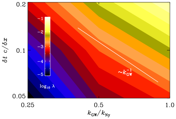
Figure 1: Dependence of the decay rate of the Beltrami field solution due to numerical error, $\lambda$, on $k_{\rm GW}/k_{\rm Ny}$ and $\delta t\,c/\delta x$. Blue (yellow) shades indicate low (high) numerical errors. The error is high when $k_{\rm GW}$ is close to the Nyquist wavenumber and $\delta t$ is large. The scaling $\delta t\,c/\delta x\propto(k_{\rm GW}/k_{\rm Ny})^{-1}$ is indicated by a white solid line (colour online).

Figure 2: Scaling of the decay rate of the Beltrami field solution due to numerical error, $\lambda$, with $k_{\rm GW}/k_{\rm Ny}$ (left panel) for $\delta t\,c/\delta x=0.05$ (straight line), $0.1$ (dotted line), and $0.2$ (dashed line), and with $\delta t\,c/\delta x$ (right panel) for $k_{\rm GW}/k_{\rm Ny}=0.25$ (straight line), $0.5$ (dotted line), and $1.0$ (dashed line). Cubic scalings are indicated by the straight lines.

3.3 Timestep constraint for approach I in a turbulent case

We now present an example where the timestep constraint becomes particularly apparent when directly integrating the GW equation. As alluded to in the introduction, this is the case when GWs are being sourced by turbulent stresses, and we use the approach I. We consider here the case of decaying helical magnetic turbulence. This case was originally considered in the cosmological context using just an irregular magnetic field and no flow as the initial condition (Brandenburg et al., 1996; Christensson et al., 2001; Banerjee and Jedamzik, 2004). In this context, one can argue that the magnetic field at scales larger than the injection scale must be causally related. This, together with the solenoidality of the magnetic field, leads to a $k^{4}$ subinertial range spectrum (Durrer and Caprini, 2003). The $E_{\rm M}(k,t)\propto k^{4}$ scaling corresponds to $\varOmega_{\rm M}(k,t)\propto k^{5}$. The magnetic field is strong and the fluid motions are just the result of the Lorentz force. The $k^{4}$ subinertial range spectrum is then followed by a $k^{-2}$ weak turbulence spectrum at high wavenumbers (Brandenburg et al., 2015). The normalised wavenumber where the change of behaviour occurs, is the peak wavenumber, $k_{*}$. For an initial $k^{4}$ spectrum, the magnetic field undergoes inverse cascading such that the magnetic energy spectrum is self-similar and obeys

$$\varOmega_{\rm M}(k,t)/k\,=\,\phi_{\rm M}\left(k\xi_{\rm M}(t)\right),$$ (51)

where $\phi_{\rm M}$ is a generic function (Christensson et al., 2001; Brandenburg and Kahniasvhili, 2017) and $\xi_{\rm M}(t)$ is the magnetic integral scale given by (99).

In figure 3 we show, for three different times, the normalised magnetic and GW energy spectra, obtained following approach I, for an expanding universe, so we have ${\cal G}(t)=6/t$ on the right-hand side of (30), and $t=1$ is the initial normalised time, which refers to the starting time of generation. Independent of the value of $\delta t$, the peak of $\varOmega_{\rm M}(k,t)/k$ is seen to propagate gradually towards smaller $k$. This is the inverse cascade owing to the presence of magnetic helicity (Pouquet et al., 1976; Biskamp and Müller, 1999; Christensson et al., 2001). Note that the peak of the spectrum always has the same height. This is compatible with (51). The ratio of $\varOmega_{\rm M}(t)/\varOmega_{\rm GW}(t)$ changes from about 100 at early times to about 20 at the last time as the magnetic field decays, while $\varOmega_{\rm GW}(t)$ stays approximately constant.

Let us now focus on the comparison of solutions for different Courant numbers, $\delta t\,c/\delta x=0.23$, $0.12$, and $0.05$ in figure 3. While the magnetic energy spectra are virtually identical for different $\delta t$, even for high wavenumbers, the GW spectra are not. There is a dramatic loss of power at large $k$, when $\delta t\,c/\delta x=0.23$. A value of $\delta t\,c/\delta x=0.8$ was always found to be safe as far as the hydrodynamics is concerned, but this is obviously not small enough for the GW solution. This is a surprising result that may not have been noted previously.

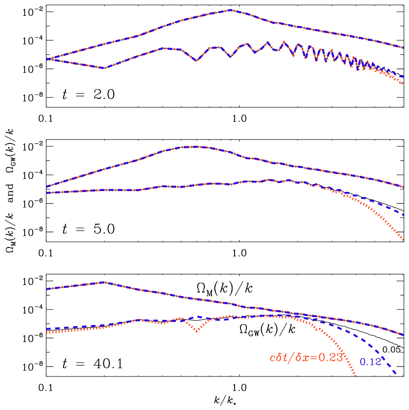
Figure 3: GW (lower curves) and magnetic (upper curves) energy spectra at three different normalised conformal times, $t=2$ (top panel), $5$ (middle panel), and $40$ (bottom panel), which are normalised with the time when the turbulence source turns on, i.e., $t_{*}$. Each panel shows three different Courant numbers: $\delta t\,c/\delta x=0.23$ (red dotted lines), 0.12 (blue dashed lines), and 0.05 (black solid lines). The wavenumbers are normalised with the normalised peak wavenumber $k_{\ast}$, at the starting time of generation. In this simulation, $k_{\ast}=10$, and the total initial magnetic field energy density is $\varOmega_{\rm M}\,(t=1)\approx 0.123$ (colour online).

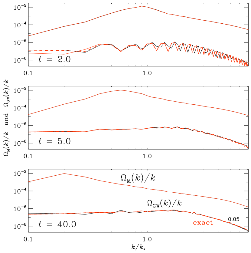
Figure 4: Same as figure 3, but now comparing the case with $\delta t\,c/\delta x=0.05$ (black solid lines), using approach I, with the analytic solution assuming constant ${\cal G}(t)T_{ij}(\bm{x},t)$, in time, between consecutive timesteps (red solid line), which corresponds to approach  II, here referred to as “exact”, using $\delta t\,c/\delta x=0.8$. The red dashed lines indicate the spectrum computed from the conformal time derivatives of the strains, $\varOmega^{\rm h^{\prime}}_{\rm GW}(k,t)/k$ (colour online).

Table 2: Dependence of the decay rate of the numerical error $\lambda$ on $k_{\rm GW}/k_{\rm Ny}$ and $\delta t\,c/\delta x$ for hydromagnetically driven GWs. Dashes indicate that the decay rate was too small compared with the fluctuations and could not be determined.

$\delta t\,c/\delta x$ $k_{\rm GW}/k_{\rm Ny}=1/4$ 1/2 1 0.23 0.012 0.16 1.1 0.12 – 0.015 0.12 0.05 – – 0.006

In figure 4, we show that the solution with $\delta t\,c/\delta x\mathrel{\mathchoice{\vbox{\offinterlineskip\halign{\hfil$\displaystyle#$\hfil\cr<\cr\sim\cr}}}{\vbox{\offinterlineskip\halign{\hfil$\textstyle#$\hfil\cr<\cr\sim\cr}}}{\vbox{\offinterlineskip\halign{\hfil$\scriptstyle#$\hfil\cr<\cr\sim\cr}}}{\vbox{\offinterlineskip\halign{\hfil$\scriptscriptstyle#$\hfil\cr<\cr\sim\cr}}}}0.05$ agrees perfectly with that of approach II at $\delta t\,c/\delta x\mathrel{\mathchoice{\vbox{\offinterlineskip\halign{\hfil$\displaystyle#$\hfil\cr<\cr\sim\cr}}}{\vbox{\offinterlineskip\halign{\hfil$\textstyle#$\hfil\cr<\cr\sim\cr}}}{\vbox{\offinterlineskip\halign{\hfil$\scriptstyle#$\hfil\cr<\cr\sim\cr}}}{\vbox{\offinterlineskip\halign{\hfil$\scriptscriptstyle#$\hfil\cr<\cr\sim\cr}}}}0.8$. The additional cost in performing Fourier transforms at every timestep, used in approach II, is easily outweighted by the more than 10 times longer timestep, when comparing to approach I. We also show the comparison between the actual GW energy spectrum, $\varOmega_{\rm GW}(k,t)$; see (21), and the spectrum obtained from conformal time derivatives, $\varOmega^{h^{\prime}}_{\rm GW}(k,t)$; see (85). These two spectra become more similar for large wavenumbers and for longer times.

To see whether the observed degradation using approach I; see figure 3, is compatible with what has been seen for the monochromatic Beltrami field, we determine again the decay rates for three wavenumbers of the spectral GW amplitude. The result is given in table LABEL:TresDNS. We see that, although the scalings with $k_{\rm GW}$ and $\delta t$ are compatible with what has been seen in section 3.2 for the Beltrami field, the actual values of $\lambda$ are about 12 times larger. The reason for this is not clear at this point.

In addition to the numerical error discussed above, when computing the solution using approach I, we found a numerical instability that is distinct from the usual one invoked in connection with the CFL condition. This new instability emerges when the accuracy of the solution is already strongly affected by the length of the timestep, namely for $\delta t\,c/\delta x\,\mathrel{\mathchoice{\vbox{\offinterlineskip\halign{\hfil$\displaystyle#$\hfil\cr>\cr\sim\cr}}}{\vbox{\offinterlineskip\halign{\hfil$\textstyle#$\hfil\cr>\cr\sim\cr}}}{\vbox{\offinterlineskip\halign{\hfil$\scriptstyle#$\hfil\cr>\cr\sim\cr}}}{\vbox{\offinterlineskip\halign{\hfil$\scriptscriptstyle#$\hfil\cr>\cr\sim\cr}}}}\,0.46$, which is still well within the range of what would normally (in hydrodynamics) be numerically stable. The problem appears at late times, after the GW spectrum has long been established. This new numerical error manifests itself as an exponential growth that is seen first at large wavenumbers and then at progressively smaller ones; see figure 5. Our earlier studies have shown that this problem cannot be controlled by adding explicit diffusion to the GW equation. Given that the solution is already no longer accurate for this length of the timestep, this numerical instability was not worth further investigation, but it highlights once again the surprising differences in the numerical behaviour of wave and fluid equations.

Figure 5: Late time numerical instability for $\delta t\,c/\delta x=0.46$ seen in the temporal evolution of $\varOmega_{\rm GW}(k,t)/k$ after $t=6$ for $k/k_{*}=7.2$ (solid), 3.6 (dotted), 1.8 (dashed), and 0.4 (dash-dotted). The spectra shown are normalised with the total GW energy density shortly after the start of the simulation, at $t\mathrel{\mathchoice{\vbox{\offinterlineskip\halign{\hfil$\displaystyle#$\hfil\cr>\cr\sim\cr}}}{\vbox{\offinterlineskip\halign{\hfil$\textstyle#$\hfil\cr>\cr\sim\cr}}}{\vbox{\offinterlineskip\halign{\hfil$\scriptstyle#$\hfil\cr>\cr\sim\cr}}}{\vbox{\offinterlineskip\halign{\hfil$\scriptscriptstyle#$\hfil\cr>\cr\sim\cr}}}}1$, $\varOmega_{\rm GW}(k,t)/k\varOmega_{\rm GW}(t\mathrel{\mathchoice{\vbox{\offinterlineskip\halign{\hfil$\displaystyle#$\hfil\cr>\cr\sim\cr}}}{\vbox{\offinterlineskip\halign{\hfil$\textstyle#$\hfil\cr>\cr\sim\cr}}}{\vbox{\offinterlineskip\halign{\hfil$\scriptstyle#$\hfil\cr>\cr\sim\cr}}}{\vbox{\offinterlineskip\halign{\hfil$\scriptscriptstyle#$\hfil\cr>\cr\sim\cr}}}}1)$. The normalised peak wavenumber is $k_{\ast}=10$, and the total initial magnetic energy density is $\varOmega_{\rm M}\,(t=1)\approx 0.123$.

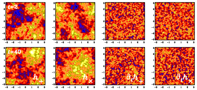
Figure 6: $xy$ cross-sections through $z=0$ of $h_{+}(\bm{x},t)$, $h_{\times}(\bm{x},t)$, and the normalised conformal time derivatives, $h_{+}^{\prime}(\bm{x},t)=\upartial_{t}h_{+}(\bm{x},t)$, and $h_{\times}^{\prime}(\bm{x},t)=\upartial_{t}h_{+}(\bm{x},t)$, at $t=2$ (upper row) and $t=40$ (lower row). The simulation parameters are the same as in figures 3 and 4 (colour online).

Looking again at the GW energy spectra at early times, figures 3 and 4, we see wiggles in the spectrum at $t=2$ (top panel). One might be concerned that these are caused by numerical artifacts, but the spatial distributions of physical $h_{+}(\bm{x},t=2)$ and $h_{\times}(\bm{x},t=2)$ look smooth; see figure 6. Thus, the wiggles in $\varOmega_{\rm GW}(k,t)/k$ are not artificial, but presumably related to the finite domain size and the way the initial condition for the magnetic field, $\varOmega_{\rm M}\,(k,t=1)/k$ is posed using combined $k^{4}$ and $k^{-2}$ power laws, for small and large wavenumbers respectively. They might appear as a transient effect in the evolution from the initially vanishing GW energy density to the shape observed for later times. Indeed, at late times the wiggles disappear.

4 Can the timestep cause artifacts in hydrodynamic and MHD turbulence?

There have been reports in the literature that the length of the timestep can affect the convergence properties of solutions of incompressible hydrodynamic simulations (Snellman et al., 2015). In the present compressible MHD simulations, however, no obvious side effects of increasing the length of the timestep within the standard CFL condition have been seen. However, there could be subtle effects. Here we investigate two possibilities. The first is the bottleneck effect in hydrodynamic turbulence, which refers to the kinetic energy spectrum, $\varOmega_{\rm K}(k,t)/k$, slightly shallower than the Kolmogorov $k^{-5/3}$ spectrum. This phenomenon is explained by the inability of triad interactions with modes in the dissipative subrange to dispose of turbulent energy from the end of the inertial range (Falkovich, 1994). This also has subtle effects on the growth rate of turbulent small-scale dynamos (see Brandenburg et al., 2018, hereafter referred to as BHLS). The second possible subtlety is a modification of the magnetic energy spectrum, $\varOmega_{\rm M}(k,t)/k$, during the kinematic growth phase. This problem of a kinematic small-scale dynamo is closest to our GW experiment in that both problems are linear and there is no turbulent cascade in either of the two problems. We begin with the first possibility.

The description in this section refers only to MHD turbulence and, for convenience, the usual non-normalised and physical variables are used for comparison with other works (e.g., $k$ refers to dimensional physical wavenumbers), instead of the normalised variables that are useful in the context of GWs. As in previous sections, however, we continue to show magnetic and kinetic energy spectra in terms of $\varOmega_{\rm M,K}(k,t)/k$.

In the simulations of BHLS, turbulence was being forced at low wavenumbers using an explicit forcing function $\bm{f}(\bm{x},t)$ on the momentum equation. It drives modes in a narrow band of wavenumbers. We consider here run D of BHLS, where driving was applied at wavenumbers between 1.4 and 1.8 times the lowest wavenumber of the domain, $k_{\min}=2\pi/L$ of a cubic domain of size $L^{3}$. The magnetic Reynolds number based on the average wavenumber was about $540$.

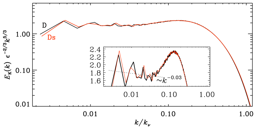
Figure 7: Comparison of the kinetic spectrum compensated with the usual Kolmogorov inertial scaling $k^{-5/3}\epsilon_{\rm K}^{2/3}$, for run D (black line) of BHLS with those of a continuation of this run with a four times shorter timestep (run Ds, red line). The inset shows the compensated spectra on a linear scale. The dotted line shows the expected inertial range correction proportional to $k^{-0.03}$ (Anselmet, 1984; She and Leveque, 1994). The physical wavenumbers are normalised with the dissipation wavenumber $k_{\nu}$. Both spectra are time-averaged after compensating against the exponential growth (colour online).

The important point of BHLS was to show that the bottleneck effect is independent of the forcing wavenumber, provided that the effective forcing wavenumber is used in the definition of the magnetic Reynolds number. Here we demonstrate that the bottleneck is not affected by the length of the timestep. Technically, the simulations presented in this section are done with magnetic fields included, but the field is at all scales still extremely weak, so for all practical purposes we can consider those as hydrodynamic simulations. The result is shown in figure 7, where we compare run D of BHLS, which uses a timestep of $\delta t\,c_{\rm s}/\delta x=0.6$, with a new one called run Ds, where ‘s’ indicates that the timestep is shorter, such that now $\delta t\,c_{\rm s}/\delta x=0.15$, where $c_{\rm s}$ refers to the sound speed. Both spectra fall off in the same way as $k$ approaches the viscous cutoff wavenumber $k_{\nu}=(\epsilon_{\rm K}/\nu^{3})^{1/4}$, where $\epsilon_{\rm K}$ is the mean kinetic energy injection rate per unit mass, and $\nu$ is the kinematic viscosity.

It turns out that there is no difference in the energy spectrum relative to run D, where the timestep obeys $\delta t\,c_{\rm s}/\delta x=0.60$. Thus, the artifacts reported in the present paper, namely the excessive damping of power at high wavenumbers, seem to be confined to the GW spectrum and do not affect in any obvious way the properties of the energy spectrum of MHD turbulence.

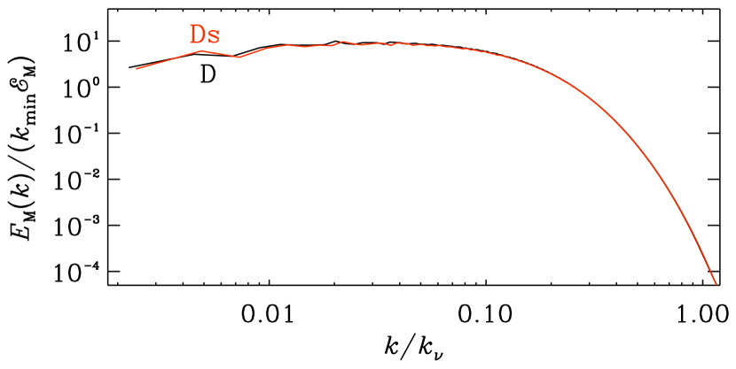
Figure 8: Comparison of the magnetic energy spectrum, $\varOmega_{\rm M}(k)/k$, normalised with the total magnetic energy ${\cal E}_{\rm M}$, for run D (black line) of BHLS with that of a continuation of this run with a four times shorter timestep (run Ds, red line) (colour online).

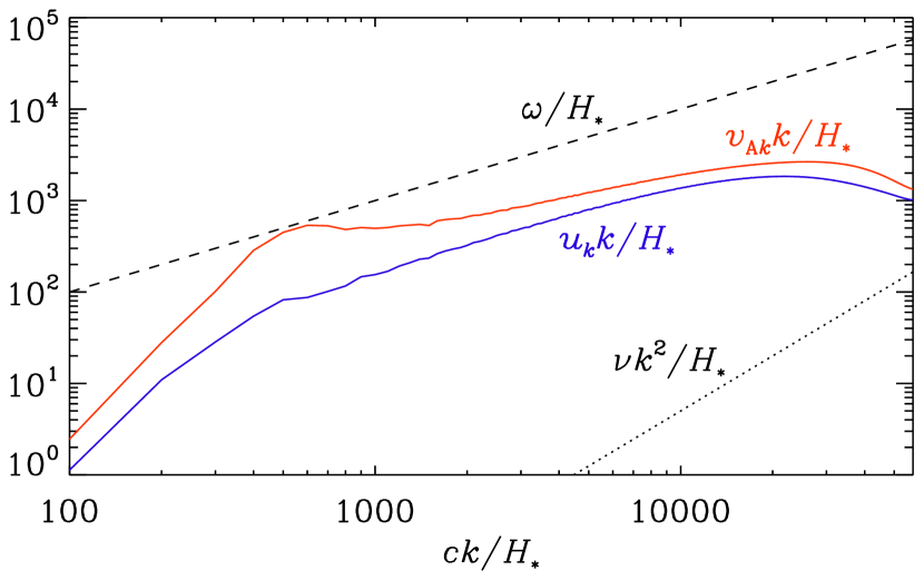
Figure 9: Comparison of the GW frequency $\omega=ck$ with the turnover rate $u_{k}(k)\,k$ of the turbulence, the turbulent Alfvén rate $v_{{\rm A}k}(k)\,k$, and the viscous damping rate $\nu k^{2}$ at normalised wavenumber $ck/H_{*}$. Note that all frequencies in the plot are normalised with $H_{*}$ (colour online).

Next, let us look at the magnetic energy spectrum during the kinematic stage. Again, we compare run D of BHLS with our new run Ds. The result is shown in figure 8, where we see virtually no difference between the two curves. In this sense, the idea that the sharp decay of the MHD energy spectra at higher wavenumbers is being masked by the forward cascade of energy may not be borne out by the simulations. However, it is possible that the spreading of energy across wavenumbers is not so much the result of nonlinearity, which is indeed unimportant in the kinematic stage of a dynamo, but that it is due to the fact that the induction equation has non-constant coefficients. This leads to mode coupling, as has been seen in other turbulent systems during the linear stage. An example is the Bell instability (Bell, 2004), where significant spreading of energy across different modes has been observed (see, for example, figure 4 of Rogachevskii et al., 2012).

The lack of any noticeable high wavenumber artifacts in MHD turbulence can simply be explained by the absence of relatively rapid oscillations in MHD flows, compared to GW oscillations, which are proportional to $c$. To demonstrate this, we compare in figure 9 the GW frequency $\omega=ck$ with the turbulent turnover rate $u_{k}(k)k$, the turbulent Alfvén rate $v_{{\rm A}k}(k)k$, and the viscous damping rate $\nu k^{2}$ at wavenumber $k$ for a simulation of GWs at $1152^{3}$ mesh points, a Reynolds number, Re = $u_{\rm rms}/\nu k$ of about 1000, and a magnetic Reynolds number Rm = Re, so that $\nu=\eta$. Here, we use the relations $u_{k}(k)=\sqrt{2E_{\rm K}(k)}$, and $v_{{\rm A}k}(k)=\sqrt{2E_{\rm M}(k)}$ for the $k$-dependent turbulent velocity and the $k$-dependent Alfvén speed. Note that $\max(v_{{\rm A}k}(k)\,k)$, at $ck/H_{*}\approx 3\cdot 10^{-4}$, is about 30 times smaller than $\omega=ck$, and the difference is bigger for larger values of $k$. This shows that from an accuracy point of view, the timestep could well be 30 times longer before the accuracy of MHD begins to be affected.

5 Conclusions

Our work has identified an important aspect that constrains the length of the timestep in numerical solutions of the linearised GW equation through approach I in a more stringent way than what is known in the more familiar MHD context. In this approach, the wave equation is integrated in the same way as the MHD equations. The resulting numerical error affects the GW spectrum at high wavenumbers in a systematic way, which may have gone unnoticed in earlier investigations.

Similar numerical errors do not seem to affect the hydromagnetic energy spectra, which could be a consequence of a direct energy cascade. It therefore appears that the direct energy cascade is insensitive to numerical errors in hydrodynamic and hydromagnetic turbulence. As discussed, fast turbulent MHD waves might have very small amplitudes due to the viscous cutoff, which becomes dominant in the range of high frequencies (see figure 9). On the other hand, this cutoff is not present in the GW oscillations. This allows the presence of waves with very high frequencies that require very small $\delta t$ to accurately represent the high frequency oscillations numerically. A particularly interesting aspect of numerical solutions of turbulence is the bottleneck effect, i.e., a shallower fall-off of spectral energy just before turbulence disposes of its energy in the viscous dissipative subrange (Kaneda et al., 2003; Haugen and Brandenburg, 2006, BHLS). One might therefore be concerned that this bottleneck itself could be the result of numerical artifacts by a finite timestep. However, we have now shown that this is not the case and that the height of the bottleneck is independent of the length of the timestep. Nevertheless, there could be other effects, especially in strongly compressible turbulence, where short timescales play a role and the solution might contain errors for timesteps below the CFL condition.

We conclude that, to obtain the correct energy spectrum at high wavenumbers with approach I, it is essential to compute solutions with rather small timesteps of just a few percent of the CFL condition. This makes reasonably accurate GW spectra (where the decay rate is less than 1% of the Hubble rate, i.e., the case with $\delta t\,c/\delta x=0.05$ in figure 3) by at least a factor of 10 more costly than what would naively be expected. In multiphysics systems, as in our case, where we solve coupled MHD equations and linearised Einstein field equations, it becomes even more important to lower the upper bound on $\delta t$, since this is affecting the duration of the numerical simulation of the whole system of equations. With approach II, however, accurate solutions have been found at ordinary timestep lengths with $C_{\rm CFL}=0.8$. The less stringent requirement on accuracy is due to the fact that the GW solution is not numerically integrated, and the oscillations are represented analytically between subsequent timesteps. This allows the representation of very high frequency oscillations, even if $\delta t$ is not small enough to numerically represent these oscillations accurately. High resolution runs have now been carried out with this scheme for a range of cases with initial magnetic field and also for cases where hydrodynamic or hydromagnetic turbulence is driven during a brief episode of stochastic forcing either in the momentum equation or in the induction equation. Those results are being reported in a separate publication (Roper Pol et al., 2019).

Appendix A Normalised GW equation

We present here the detailed derivation of the normalised GW equation (6). The spatial components of the background metric for an isotropic and homogeneous universe are described by the Friedmann–Lemaître–Robertson–Walker (FLRW) metric $\gamma_{ij}(t)=a^{2}(t)\delta_{ij}$, for signature $(-++\,\,+)$, where $a(t)$ is the scale factor, and $\delta_{ij}$ is the Kronecker delta. Assuming small tensor-mode perturbations $a^{2}(t)h_{ij}^{\rm phys}(\bm{x},t)$, where $h_{ij}^{\rm phys}(\bm{x},t)$ are also called strains, over the FLRW metric, such that the resulting metric tensor is $g_{ij}(\bm{x},t)=\gamma_{ij}(t)+a^{2}(t)h_{ij}^{\rm phys}(\bm{x},t)=a^{2}(t)[\delta_{ij}+h_{ij}^{\rm phys}(\bm{x},t)]$, the GW equation in physical space and time coordinates, governing the physical strains is

$$\biggl{(}{\upartial^{2}\over\upartial t_{\rm phys}^{2}}+3H(t){\upartial\over\upartial t_{\rm phys}}-c^{2}\nabla^{2}_{\text{phys}}\biggr{)}h_{ij,\text{phys}}^{\rm TT}(\bm{x},t)\,=\,\frac{16\pi G}{c^{2}}T^{\text{TT}}_{ij,\text{phys}}(\bm{x},t)\,,$$ (52)

where $c$ is the speed of light, $G$ is Newton’s gravitational constant, $H(t)=\dot{a}/a=a^{\prime}/a^{2}$ is the Hubble rate, where dot represents physical time derivative, and prime denotes conformal time derivative; and TT is the transverse and traceless projection described in section 2.2. The physical space and time coordinates are related to the comoving space and conformal time coordinates through $\bm{x}_{\rm phys}=a(t)\bm{x}$, $a(t){\bm\nabla}_{\text{phys}}={\bm\nabla}$, and ${\mathrm{d}}t_{\text{phys}}=a(t){\mathrm{d}}t$. The physical stress-energy tensor is related to the comoving stress-energy tensor through $a^{4}(t)T_{ij,\text{phys}}^{\text{TT}}(\bm{x},t)=T_{ij}^{\text{TT}}(\bm{x},t)$. The comoving variables are defined to take into account the expansion of the universe, and the corresponding dilution of the energy density. Note that the physical wavevector in Fourier space, $\bm{k}_{\rm phys}$, is also related to the comoving wavevector as $a(t)\bm{k}_{\rm phys}=\bm{k}$. This also affects the frequency $f_{\rm phys}$, which is related to $k_{\rm phys}=|\bm{k}_{\rm phys}|$ through the dispersion relation $2\pi f_{\rm phys}=ck_{\rm phys}$. Hence, the comoving frequency is $a(t)f_{\rm phys}=f$.

The stress-energy has been defined as a comoving variable. This affects the hydromagnetic fields that are part of the stress-energy tensor, i.e., $p,\rho,\bm{u},\bm{B}$, and the fields that can be obtained as a function of the hydromagnetic fields, e.g., $\bm{J}$ or $\boldsymbol{S}$, which appear in section 2.5. Hence, all these fields are defined also as comoving fields, consistently with the $a^{-4}(t)$ dilution of the stress-energy tensor. This is described in more detail in Subramanian (2016).

A.1 Using conformal time

The GW equation (52) can be expressed in terms of comoving space and conformal time coordinates, comoving stress-energy tensor, and scaled strains $h_{ij}^{\text{TT}}(\bm{x},t)=a(t)h_{ij,\text{phys}}^{\text{TT}}(\bm{x},t)$ as

$$\left({\upartial^{2}\over\upartial t^{2}}-{a^{\prime\prime}\over a}(t)-c^{2}\nabla^{2}\right)h_{ij}^{\text{TT}}(\bm{x},t)\,=\,\frac{16\pi G}{a(t)c^{2}}T_{ij}^{\text{TT}}(\bm{x},t)\,.$$ (53)

When the universe was dominated by radiation (approximately until the epoch of recombination), the pressure was dominated by radiation, and given by the relativistic equation of state $p=\rho c^{2}/3$, so the speed of sound is $c_{\rm s}=c/\sqrt{3}$. This relation allows us to obtain the solution to the Friedmann equations (see Friedmann, 1922), which results in a linear evolution of the scale factor with conformal time, i.e., $a(t)=C_{t}t$, for some constant $C_{t}$, such that $a^{\prime\prime}=0$. This simplifies equation (53) to

$$\left({\upartial^{2}\over\upartial t^{2}}-c^{2}\nabla^{2}\right)h_{ij}^{\text{TT}}(\bm{x},t)\,=\,\frac{16\pi G}{a(t)c^{2}}T_{ij}^{\text{TT}}(\bm{x},t)\,.$$ (54)

The stress-energy tensor can be normalised as $\bar{T}_{ij}^{\text{TT}}(\bm{x},t)=T_{ij}^{\text{TT}}(\bm{x},t)/{\cal E}_{\rm rad}^{*}$, where the radiation energy density during the radiation-dominated epoch is equal to the total energy density of the universe, given by the critical energy density derived from the Friedmann equations,

$${\cal E}_{\rm rad}^{*}\,=\,\frac{\pi^{2}g_{*}(T_{*})(k_{\rm B}T_{*})^{4}}{30\,(\hbar c)^{3}}\,=\,{\cal E}_{\rm crit}^{*}\,=\,\rho_{*}c^{2}\,=\,\frac{3H_{*}^{2}c^{2}}{8\pi G}\,,$$ (55)

where $T_{*}$, $g_{*}(T_{*})$, and $H_{\ast}$ are the temperature, the number of relativistic degrees of freedom, and the Hubble rate, respectively, during the time of generation, and $k_{\rm B}$ and $\hbar$ are the Boltzmann and the reduced Planck constants. In our simulations, we choose the electroweak phase transition as the starting time of turbulence generation. The Hubble parameter at the electroweak phase transition is given by (55) as

$$H_{*}\,\approx\,2.066\cdot 10^{10}\ {\rm s}^{-1}\left(T_{*}\over 100\ {\rm GeV}\right)^{2}\left(g_{*}(T_{*})\over 100\right)^{1/2},$$ (56)

where an energy of $k_{\rm B}T_{*}=100\,{\rm GeV}$, and the corresponding relativistic degrees of freedom $g_{*}(T_{*})=100$, have been used to get an estimate of the Hubble rate, $H_{*}$, at the electroweak phase transition. The exact temperature at the electroweak phase transition is uncertain, so it is left as a parameter in (56).

A.2 Case I: Static universe

The resulting expression for GWs in a static universe, after normalisation of $\bar{T}_{ij}^{\rm TT}(\bm{x},t)$, is

$$\left({\upartial^{2}\over\upartial t^{2}}-c^{2}\nabla^{2}\right)h_{ij}^{\rm TT}(\bm{x},t)\,=\,6H_{\ast}^{2}\bar{T}_{ij}^{\rm TT}(\bm{x},t)\,.$$ (57)

This is the equation that we use for a non-expanding universe, where we can shift the time coordinate to zero at the starting time of generation due to the absence of the scale factor $a(t)$ in the equation, to simplify the resulting expressions. Comoving space and conformal time coordinates are the same as the physical coordinates in this case, and likewise for physical and scaled strains. Hence, the solution is readily given in terms of physical quantities.

A.3 Case II: Expanding universe

For more realistic cosmological computations of GWs generated by hydromagnetic turbulence during the radiation-dominated epoch, the expansion of the universe has to be taken into account. For this purpose, it is useful to normalise $t$ with respect to the conformal time of generation $t_{*}$, which corresponds to the time where the turbulent motions sourcing GWs are assumed to begin to be generated, such that $\bar{t}=t/t_{*}$. The Hubble parameter at the starting time of generation $H_{*}$ can be related to $C_{t}$ via $C_{t}=H_{*}a_{*}^{2}$, which allows us to express the initial time of generation as $t_{*}=\left(H_{*}a_{*}\right)^{-1}$. The Laplacian operator is normalised as $\bar{\nabla}^{2}=c^{2}\nabla^{2}/H_{*}^{2}$. As previously, the normalisation of the Laplacian operator implies the normalisation of wavenumber $\bar{k}=ck/H_{*}$, and the frequency $\bar{f}=f/H_{*}$, related to $\bar{k}$, through the dispersion relation $2\pi\bar{f}=\bar{k}$. This normalisation allows us to express the evolution of the scale factor as $a(\bar{t})=$ $a_{*}\bar{t}$, where $a_{*}$ is the scale factor at the starting time of generation. For a flat FLRW model, the scale factor $a(t)$ at any time $t$ is only defined relative to its value at any other time of the universe history (Weinberg, 2008). The usual convention is to set $a_{0}=1$ at the present time. However, for the present purpose, it is more convenient to set $a_{*}=1$, at the initial time of the simulation $\bar{t}=1$, i.e., at the electroweak phase transition. This needs to be taken into account when the characteristic amplitude and the energy density obtained from the calculations are expressed as observables at the present time, as described in appendix B. The expansion of the universe is assumed to be adiabatic, such that $g_{S}(T)T^{3}a^{3}(T)$ is constant, where $g_{S}(T)$ is the number of adiabatic degrees of freedom at temperature $T$. This allows us to compute the scale factor at the present time $a_{0}$, relative to $a_{*}=1$, as

$$a_{0}\,\approx\,1.254\cdot 10^{15}\left(T_{*}\over 100\ {\rm GeV}\right)\left(g_{S}(T_{*})\over 100\right)^{1/3},$$ (58)

where $g_{S}(T_{*})$ is the number of adiabatic degrees of freedom during the period of generation. Again, the exact values of $g_{S}(T_{*})$ and $T_{*}$ at the electroweak phase transition are uncertain, and the previous expression allows to use different values. After this normalisation, the GW equation (54) reduces to the normalised GW equation.

$$\left({\upartial^{2}\over\upartial\bar{t}^{2}}-\bar{\nabla}^{2}\right)h_{ij}^{\rm TT}(\bar{\bm{x}},\bar{t})\,=\,{6\over\bar{t}}\bar{T}_{ij}^{\rm TT}(\bar{\bm{x}},\bar{t})\,,$$ (59)

where $\bar{\bm{x}}$ are also normalised comoving space coordinates, related to comoving space coordinates $\bar{\bm{x}}=H_{*}\bm{x}/c$. After removing the bars, we recover (6).

Appendix B Computation of the characteristic amplitude, the GW energy density and the spectral functions.

We present here a detailed description of the characteristic amplitude and GW energy density, defined in section 2.4, how to relate these quantities to observables at the present time, and how to compute them from the numerical simulations. From now on, to simplify notation, the TT projection will be assumed since only TT projected strains, i.e., the gauge invariant strains, are physically relevant. We also define the spectral functions $S_{h}(k,t)$, $S_{\dot{h}}(k,t)$, and $A_{\dot{h}}$, that are used in section 2.4 to describe the spectral characteristic amplitude $h_{\rm rms}(k,t)$, the GW energy spectrum $\varOmega_{\rm GW}(k,t)$, and the helical GW spectrum $\varXi_{\rm GW}(k,t)$. The characteristic amplitude $h_{\rm rms}(t)$, defined in (18) in terms of the physical strains, can also be expressed in terms of the scaled strains and normalised conformal time as

$$h_{\rm rms}^{2}(t)\,=\,\frac{1}{2t^{2}}\langle h_{ij}(\bm{x},t)h_{ij}(\bm{x},t)\rangle\,,$$ (60)

where angle brackets indicate volume averaging in physical space. This expression can be computed directly from the solutions that we obtain from the code, following the methodology presented in section 2.6. In our simulations, we assume MHD turbulence sourcing GWs from the time of generation until the end of the radiation-dominated epoch, at recombination. At this point, we assume that there are no sources affecting the primordial stochastic GW background, such that the latter freely propagates from this time on. In the absence of GW generation, the physical strains damp as $a^{-1}(t)$ with the expansion of the universe, as can be inferred from (6) with $T_{ij}=0$. The observable characteristic amplitude at the present time, $h_{\rm rms}^{0}$, is related to the final result obtained at the end of the simulation (denoted by superscript “end”) as

$$h_{\rm rms}^{0}\,=\,h_{\rm rms}^{\rm(end)}a^{\rm(end)}a_{0}^{-1}\,=\,\sqrt{{\textstyle{1\over 2}}\langle h_{ij}(\bm{x},t)h_{ij}(\bm{x},t)\rangle^{\rm(end)}}\,a_{0}^{-1}\,,$$ (61)

where $a_{0}$ is the scale factor at the present time, scaled such that the scale factor at the starting time of generation is unity; see (58), and $a^{\rm(end)}$ is the scale factor at the end of the simulation. We have used the fact that the scale factor is $a(t)=t$ in normalised units (see appendix A for details), to simplify the previous equation.

The mean GW energy density ${\cal E}_{\rm GW}(t)$ is defined in (19) in terms of the derivative of the physical strains with respect to physical time $\dot{h}_{ij}^{\rm phys}(\bm{x},t)$ and the normalised GW energy density is $\varOmega_{\rm GW}(t)={\cal E}_{\rm GW}(t)\left/{\cal E}_{\rm rad}^{*}\right.$, where the radiation energy density at the starting time of generation, ${\cal E}_{\rm rad}^{*}$, is defined in (55).

In the case of an expanding universe, it is also useful to define normalised $\varOmega_{\rm GW}^{0}(t)=\left.{\cal E}_{\rm GW}(t)\right/{\cal E}_{\rm crit}^{0}$, where ${\cal E}_{\rm crit}^{0}=3H_{0}^{2}c^{2}\left/\left(8\pi G\right)\right.$ is the critical energy density at present time, $H_{0}$ being the current Hubble parameter. The value of the Hubble parameter at the present time is customarily expressed as $H_{0}=100\,h_{0}\,{\rm km}\,{\rm s}^{-1}\,{\rm Mpc}^{-1}$, where $h_{0}\approx 0.71$ takes into account the uncertainties of its value (Riess et al., 2011; Ade et al., 2015). To get rid of the uncertainties of $H_{0}$ in the calculations, it is common to use $h_{0}^{2}\varOmega_{\rm GW}^{0}(t)$, instead of just $\varOmega_{\rm GW}^{0}(t)$ (Maggiore, 2000). This is used to compute the present time observable GW signal generated during the early universe turbulent epoch and taking into account its dilution due to the expansion of the universe, as it has been done for $h_{\rm rms}(t)$.

We recall that the dots in (19) denote physical time derivatives. In terms of the normalised conformal time $t$ and scaled strains $h_{ij}(\bm{x},t)$, the physical time derivative of the physical strains $h_{ij}^{\rm phys}(\bm{x},t)$ is

$$\dot{h}_{ij}^{\rm phys}(\bm{x},t)\,=\,{H_{*}\over t}{\upartial\over\upartial t}\left(h_{ij}(\bm{x},t)\over t\right)\,=\,\frac{H_{*}}{t^{2}}\left(h^{\prime}_{ij}(\bm{x},t)-{h_{ij}(\bm{x},t)\over t}\right)\,.$$ (62)

Therefore, the normalised GW energy density $\varOmega_{\rm GW}^{0}(t)$ can be expressed in terms of the normalised conformal time as

$$\varOmega_{\rm GW}^{0}(t)\,=\,\frac{\left(H_{*}\left/H_{0}\right.\right)^{2}}{12t^{4}}\left[\langle h^{\prime}_{ij}h^{\prime}_{ij}\rangle+\frac{1}{t^{2}}\langle h_{ij}h_{ij}\rangle-\frac{2}{t}\langle h^{\prime}_{ij}h_{ij}\rangle\right],$$ (63)

where the explicit dependence on $\bm{x}$ and $t$ has been omitted to simplify the notation. The energy density $\varOmega^{0}_{\rm GW}(t)$ has three different contributions:

$$\varOmega_{\rm GW}^{{\rm h^{\prime}},0}(t)\,\propto\, \,\langle h^{\prime}_{ij}h^{\prime}_{ij}\rangle\,,$$ (64a)

$$\varOmega_{\rm GW}^{{\rm h},0}(t)\,\propto\, \,\langle h_{ij}h_{ij}\rangle\,=\,2t^{2}h_{\rm rms}^{2}(t)\,,$$ (64b)

$$\varOmega_{\rm GW}^{{\rm mix},0}(t)\,\propto\, \,\langle h^{\prime}_{ij}h_{ij}\rangle\,,$$ (64c)

such that $\varOmega^{0}_{\rm GW}(t)=\varOmega_{\rm GW}^{{\rm h^{\prime}},0}(t)+t^{-2}\varOmega_{\rm GW}^{{\rm h},0}(t)-2t^{-1}\varOmega_{\rm GW}^{{\rm mix},0}(t)$. Note that $\varOmega_{\rm GW}(t)$ is obtained from (63) without the prefactor $H_{*}\left/H_{0}\right.$, as well as $\varOmega^{i}_{\rm GW}(t)$, for $i$ = h^′, h, mix. The energy density dilutes as $a^{-4}$ due to the expansion of the universe. We can relate the GW energy density at the present time with the final result obtained at the end of the simulation as

$$\varOmega_{\rm GW}^{0}(t_{\rm end})t_{\rm end}^{4}a_{0}^{-4}\,=\,\varOmega_{\rm GW}^{{\rm h^{\prime}},0}(t_{\rm end})+t_{\rm end}^{-2}\varOmega_{\rm GW}^{{\rm h},0}(t_{\rm end})-2t_{\rm end}^{-1}\varOmega_{\rm GW}^{{\rm mix},0}(t_{\rm end})\,,$$ (65)

where

$$\varOmega_{\rm GW}^{{\rm h^{\prime}},0}(t_{\rm end})\,=\, \,{\left(H_{*}\left/H_{0}\right.\right)^{2}\over 12a_{0}^{4}}\langle h^{\prime}_{ij}h^{\prime}_{ij}\rangle^{\rm(end)\,},$$ (66a)

$$\varOmega_{\rm GW}^{{\rm h},0}(t_{\rm end})\,=\, \,{\left(H_{*}\left/H_{0}\right.\right)^{2}\over 12a_{0}^{4}}\langle h_{ij}h_{ij}\rangle^{\rm(end)}\,,$$ (66b)

$$\varOmega_{\rm GW}^{{\rm mix},0}(t_{\rm end})\,=\, \,{\left(H_{*}\left/H_{0}\right.\right)^{2}\over 12a_{0}^{4}}\langle h_{ij}h^{\prime}_{ij}\rangle^{\rm(end)}\,.$$ (66c)

The spectral function $S_{h}(k,t)$, used to compute the characteristic amplitude $h_{\rm rms}(k,t)$ (see section 2.4) is defined as

$$S_{h}(k,t)\,=\,\int_{\varOmega_{D}}\left(\left|\tilde{h}_{+}^{\rm phys}(\bm{k},t)\right|^{2}+\left|\tilde{h}_{\times}^{\rm phys}(\bm{k},t)\right|^{2}\right)\,k^{D-1}\,{\rm d}\varOmega_{k}\,.$$ (67)

This is the shell-integrated spectrum of ${\textstyle{1\over 2}}\tilde{h}^{\rm phys}_{ij}\tilde{h}^{\rm phys,*}_{ij}$ over all directions of $\bm{k}$, which can be expressed, using the orthogonality property of the linear polarisation basis, as $\tilde{h}^{\rm phys}_{+}\tilde{h}_{+}^{\rm phys,*}+\tilde{h}^{\rm phys}_{\times}\tilde{h}_{\times}^{\rm phys,*}$; see (10); $D$ is the number of dimensions, and $\varOmega_{D}$ is the solid angle subtended by the entire $(D-1)$–sphere, such that $\varOmega_{1}=2$, $\varOmega_{2}=2\pi$, $\varOmega_{3}=4\pi$ are, respectively, the $(D-1)$–surface of a line, a circle and a sphere. The spectral function $S_{h}(k,t)$ is expressed in terms of the scaled strains $\tilde{h}_{+,\times}(\bm{k},t)$ as

$$S_{h}(k,t)\,=\,{1\over t^{2}}\int_{\varOmega_{D}}\left(\left|\tilde{h}_{+}(\bm{k},t)\right|^{2}+\left|\tilde{h}_{\times}(\bm{k},t)\right|^{2}\right)\,k^{D-1}\,{\rm d}\varOmega_{k}\,.$$ (68)

For a non-expanding universe we can directly use (67) since scaled and physical strains are then the same. The integration over all wavenumbers of $S_{h}(k,t)$ leads to

$$\int_{0}^{\infty}S_{h}(k,t)\,{\rm d}k\,=\,\int_{-\infty}^{\infty}h_{\rm rms}^{2}(k,t)\,{\rm d}\ln k=h_{\rm rms}^{2}(t)\,.$$ (69)

This can be shown making use of the Parseval’s theorem

$$\langle h_{ij}(\bm{x},t)h_{ij}(\bm{x},t)\rangle\,=\, \,\frac{1}{L^{3}}\int_{\cal V}h_{ij}(\bm{x},t)h_{ij}(\bm{x},t)\,{\rm d}^{3}{\color[rgb]{0,0,0}\bm{x}}$$

$$=\, \,\,\sum_{\bm{k}}\tilde{h}_{ij}(\bm{k},t)\tilde{h}_{ij}^{\ast}(\bm{k},t)$$

$$=\, \,\,2\sum_{\bm{k}}\left(\tilde{h}_{+}(\bm{k},t)\tilde{h}_{+}^{*}(\bm{k},t)+\tilde{h}_{\times}(\bm{k},t)\tilde{h}_{\times}^{*}(\bm{k},t)\right)\,$$

$$=\, \,2t^{2}\int_{0}^{\infty}S_{h}(k,t)\,{\rm d}k\,=\,2t^{2}h_{\rm rms}^{2}(t)\,,$$ (70)

where ${\cal V}=L^{3}$ is the volume in physical space of length $L$.

The spectral function associated with the characteristic amplitude $h^{0}_{\rm rms}(k)$ can also be expressed as an observable at the present time, as it has been done in (61), for the physical $h_{\rm rms}(t)$.

$$h^{0}_{\rm rms}(k)\,=\,a_{0}^{-1}\sqrt{kS_{h}(k,t_{\rm end})}\,,$$ (71)

where $t_{\rm end}$ is the end time of the simulation. When we compute the observable $h_{\rm rms}$ spectrum at the present time, we are interested in its dependence on the physical wavenumber $k^{\rm phys}_{0}$ at the present time. The relation to the normalised wavenumber $k$ is given by

$$k_{0}^{\rm phys}\,=\,H_{*}a_{0}^{-1}k/c\,.$$ (72)

This shifting in wavenumbers is computed for the following spectral functions when we plot spectra as observables at the present time.

Analogous to $S_{h}(k,t)$ we define the spectral function $S_{\dot{h}}(k,t)$, with a dot, as

$$S_{\dot{h}}(k,t)\,=\,\int_{\varOmega_{D}}\left(\left|\dot{\tilde{h}}_{+}^{\rm phys}(\bm{k},t)\right|^{2}+\left|\dot{\tilde{h}}_{\times}^{\rm phys}(\bm{k},t)\right|^{2}\right)\,k^{D-1}\,{\rm d}\varOmega_{k}\,.$$ (73)

This is the shell-integrated spectrum over all directions of ${\textstyle{1\over 2}}\dot{\tilde{h}}_{ij}^{\rm phys}\dot{\tilde{h}}_{ij}^{\rm phys,*}=\dot{\tilde{h}}_{+}^{\rm phys}\dot{\tilde{h}}_{+}^{\rm phys,*}+\dot{\tilde{h}}_{\times}^{\rm phys}\dot{\tilde{h}}_{\times}^{\rm phys,*}$, defined as in (67). The corresponding spectral function for the energy spectrum $E_{\rm GW}(k,t)$ is defined as

$$E_{\rm GW}(k,t)\,=\,\frac{c^{2}}{16\pi G}S_{\dot{h}}(k,t),\hskip 22.76219pt\text{such that \ }\hskip 17.07164pt\int_{0}^{\infty}E_{\rm GW}(k,t)\,{\rm d}k\,=\,{\cal E}_{\rm GW}(t)\,,\hskip 17.07164pt$$ (74)

where, as before, the resulting mean energy density ${\cal E}_{\rm GW}(t)$ corresponds to that defined in (19), due to Parseval’s theorem, used in (70). The GW spectrum $E_{\rm GW}(k,t)$ is used to define a characteristic length scale of GWs, $\xi_{\rm GW}(t)$, and the corresponding characteristic wavenumber, $k_{\rm GW}(t)$, as

$$\xi_{\rm GW}(t)\,=\,k_{\rm GW}^{-1}(t)\,=\,\frac{1}{{\cal E}_{\rm GW}(t)}\int_{0}^{\infty}k^{-1}E_{\rm GW}(k,t)\,{\rm d}k\,.$$ (75)

Note that we have defined here $\xi_{\rm GW}$ without $2\pi$ factor, which is analogous to our definition of the magnetic and kinetic correlation lengths (see Kahniashvili et al., 2010). We also define $\varOmega_{\rm GW}^{0}(k,t)$, normalising with $H_{0}$ instead of $H_{*}$. The antisymmetric spectral function of GWs, $A_{\dot{h}}(k,t)$, in relation to the symmetric spectral function $S_{\dot{h}}(k,t)$, is defined as

$${\color[rgb]{0,0,0}i}A_{\dot{h}}(k,t)\, \,=\,\int_{\varOmega_{D}}\left(\dot{\tilde{h}}_{+}^{\rm phys}\dot{\tilde{h}}_{\times}^{{\rm phys},\ast}-\dot{\tilde{h}}_{+}^{{\rm phys},\ast}\dot{\tilde{h}}_{\times}^{\rm phys}\right)\,k^{D-1}\,{\rm d}\varOmega_{k}$$

$$\,=\,2{\color[rgb]{0,0,0}i}\int_{\varOmega_{D}}{\rm Im}\left(\dot{\tilde{h}}_{+}^{\rm phys}\dot{\tilde{h}}_{\times}^{{\rm phys},\ast}\right)\,k^{D-1}\,{\rm d}\varOmega_{k}\,,$$ (76)

where the explicit dependence on $\bm{k}$ and $t$ in the integrand has been avoided for notational simplicity. Contrary to the symmetric spectral function $S_{\dot{h}}(k,t)$, which is positive definite, $A_{\dot{h}}(k,t)$ can be positive or negative. The motivation to define $S_{\dot{h}}(k,t)$ and $A_{\dot{h}}(k,t)$ follows the description of the autocorrelation function for any second-rank tensor used in Caprini et al. (2004). The autocorrelation function for the physical time derivative of the scaled strains $\dot{\tilde{h}}_{ij}(\bm{k},t)$ is defined in terms of the symmetric and antisymmetric spectral functions as

$$\int_{\varOmega_{D}}\dot{\tilde{h}}_{ij}(\bm{k},t)\dot{\tilde{h}}^{*}_{lm}(\bm{k}^{\prime},t)\,k^{D-1}\,{\rm d}\varOmega_{k}\,=\,\frac{1}{4}\Big{[}{\cal M}_{ijlm}S_{\dot{h}}(k,t)+i{\cal A}_{ijlm}A_{\dot{h}}(k,t)\Big{]}\,,$$ (77)

where the prefactor tensors ${\cal M}_{ijlm}$, and ${\cal A}_{ijlm}$ are defined as

$${\cal M}_{ijlm}\,=\, \,P_{il}P_{jm}+P_{im}P_{jl}-P_{ij}P_{lm}\,,$$ (78)

$${\cal A}_{ijlm}\,=\, \,{\textstyle{1\over 2}}\bm{e}^{q}\left(P_{jm}\epsilon_{ilq}+P_{il}\epsilon_{jmq}+P_{im}\epsilon_{jlq}+P_{jl}\epsilon_{imq}\right)\,,$$ (79)

where $P_{ij}$ is the projection operator that appears in (4), $\bm{e}^{i}$ is the basis defined in section 2.3, and $\epsilon_{ijk}$ is the Levi-Civita tensor. The spectral function associated with the corresponding antisymmetric contribution to the energy density, $H_{\rm GW}(k,t)$, is

$$H_{\rm GW}(k,t)\,=\,\frac{c^{2}}{16\pi G}A_{\dot{h}}(k,t),\hskip 22.76219pt\text{such that \ }\hskip 17.07164pt\int_{0}^{\infty}H(k,t)\,{\rm d}k\,=\,{\cal H}_{\rm GW}(t)\,,\hskip 17.07164pt$$ (80)

where an antisymmetric or helical energy density ${\cal H}_{\rm GW}(t)$ has been defined in analogy to the energy density ${\cal E}_{\rm GW}(t)$. We also define $\varXi_{\rm GW}^{0}(k,t)$ and $\varXi_{\rm GW}^{0}(t)$ normalised with $H_{0}$.

The spectral functions $S_{\dot{h}}(k,t)$ and $A_{\dot{h}}(k,t)$ depend on the physical time derivatives of the physical strains. We want to express the spectral functions in terms of derivatives of the scaled strains with respect to conformal time. For that purpose, to compute $S_{\dot{h}}(k,t)$, we define the spectral functions $S_{h^{\prime}}(k,t)$ and $S_{\rm mix}(k,t)$ as

$$S_{h^{\prime}}(k,t)\,=\, \,\int_{\varOmega_{D}}\left(\left|\tilde{h}^{\prime}_{+}(\bm{k},t)\right|^{2}+\left|\tilde{h}^{\prime}_{\times}(\bm{k},t)\right|^{2}\right)\,k^{D-1}\,{\rm d}\varOmega_{k}\,,$$ (81)

$$S_{\rm mix}(k,t)\,=\, \,\int_{\varOmega_{D}}{\rm Re}\left(\tilde{h}_{+}\tilde{h}_{+}^{{}^{\prime}*}(\bm{k},t)+\tilde{h}_{\times}\tilde{h}_{\times}^{{}^{\prime}*}(\bm{k},t)\right)\,k^{D-1}\,{\rm d}\varOmega_{k}\,.$$ (82)

Now, using (62), we can express $S_{\dot{h}}(k,t)$ as

$$S_{\dot{h}}(k,t)\,=\,\frac{H_{*}^{2}}{t^{4}}\Big{[}S_{h^{\prime}}(k,t)+S_{h}(k,t)-2t^{-1}S_{\rm mix}(k,t)\Big{]}\,,$$ (83)

where $S_{h}(k,t)$ is defined in (67) and (68). This allows us to define, analogous to (74) and (21), the GW energy spectra

$$E_{\rm GW}^{\rm h^{\prime}}(k,t)\,=\,c^{2}S_{h^{\prime}}(k,t)\left/\left(16\pi G\right)\right.,\hskip 22.76219ptE_{\rm GW}^{\rm mix}(k,t)\,=\,c^{2}S_{\rm mix}(k,t)\left/\left(16\pi G\right)\right.,\hskip 22.76219pt$$ (84)

and the normalised spectra

$$\varOmega_{\rm GW}^{\rm h^{\prime}}(k,t)\,=\, \,kS_{h^{\prime}}(k,t)\left/\left(6H_{*}^{2}\right)\right., \varOmega_{\rm GW}^{\rm mix}(k,t)\,=\, \,kS_{\rm mix}(k,t)\left/\left(6H_{*}^{2}\right)\right.,$$ (85a)

$$\varOmega_{\rm GW}^{{\rm h^{\prime}},0}(k,t)\,=\, \,kS_{h^{\prime}}(k,t)\left/\left(6H_{0}^{2}\right)\right., \varOmega_{\rm GW}^{{\rm mix},0}(k,t)\,=\, \,kS_{\rm mix}(k,t)\left/\left(6H_{0}^{2}\right)\right..\hskip 22.76219pt$$ (85b)

For the antisymmetric spectral function we define $A_{h^{\prime}}(k,t)$, $A_{\rm mix}(k,t)$ and $A_{h}(k,t)$ as

$$A_{h^{\prime}}(k,t)\,=\, \,2\int_{\varOmega_{D}}{\rm Im}\left(\tilde{h}^{\prime}_{+}\tilde{h}_{\times}^{\prime\,\ast}\right)\,k^{D-1}\,{\rm d}\varOmega_{k}\,,$$ (86)

$$A_{\rm mix}(k,t)\,=\, \,\int_{\varOmega_{D}}{\rm Im}\left(\tilde{h}^{\prime}_{+}\tilde{h}_{\times}^{\ast}+\tilde{h}_{+}\tilde{h}^{\prime\,\ast}_{\times}\right)\,k^{D-1}\,{\rm d}\varOmega_{k}\,,$$ (87)

$$A_{h}(k,t)\,=\, \,2\int_{\varOmega_{D}}{\rm Im}\left(\tilde{h}_{+}^{\rm phys}\tilde{h}_{\times}^{\rm phys,\ast}\right)\,k^{D-1}\,{\rm d}\varOmega_{k}$$

$$=\, \,2t^{-2}\int_{\varOmega_{D}}{\rm Im}\left(\tilde{h}_{+}\tilde{h}_{\times}^{\ast}\right)\,k^{D-1}\,{\rm d}\varOmega_{k}\,,$$ (88)

such that $A_{\dot{h}}(k,t)$ can be expressed as

$$A_{\dot{h}}(k,t)\,=\,\frac{H_{*}^{2}}{t^{4}}\Big{[}A_{h^{\prime}}(k,t)+A_{h}(k,t)-2t^{-1}A_{\rm mix}(k,t)\Big{]}\,.$$ (89)

Again, this allows us to define, analogous to (80) and (22), the antisymmetric GW energy spectra

$$H_{\rm GW}^{\rm h^{\prime}}(k,t)\,=\,c^{2}A_{h^{\prime}}(k,t)\left/\left(16\pi G\right)\right.,\hskip 22.76219ptH_{\rm GW}^{\rm mix}(k,t)\,=\,c^{2}A_{\rm mix}(k,t)\left/\left(16\pi G\right)\right.,\hskip 22.76219pt$$ (90)

and the normalised spectra

$$\varXi_{\rm GW}^{\rm h^{\prime}}(k,t)\,=\, \,kA_{h^{\prime}}(k,t)\left/\left(6H_{*}^{2}\right)\right., \varXi_{\rm GW}^{\rm mix}(k,t)\,=\, \,kA_{\rm mix}(k,t)\left/\left(6H_{*}^{2}\right)\right.,$$ (91a)

$$\varXi_{\rm GW}^{{\rm h^{\prime}},0}(k,t)\,=\, \,kA_{h^{\prime}}(k,t)\left/\left(6H_{0}^{2}\right)\right., \varXi_{\rm GW}^{{\rm mix},0}(k,t)\,=\, \,kA_{\rm mix}(k,t)\left/\left(6H_{0}^{2}\right)\right..\hskip 17.07164pt$$ (91b)

Therefore, the spectral functions $\varOmega_{\rm GW}^{0}(k,t)$, $\varXi_{\rm GW}^{0}(k,t)$, and ${\cal P}(k,t)$ can be expressed as

$$\varOmega^{0}_{\rm GW}(k,t)\,=\, \,{\left(H_{*}\left/H_{0}\right.\right)^{2}\over 6t^{4}}k\Big{[}S_{h^{\prime}}(k,t)+S_{h}(k,t)-2t^{-1}S_{\rm mix}(k,t)\Big{]}\,,$$ (92)

$$\varXi^{0}_{\rm GW}(k,t)=\, \,{\left(H_{*}\left/H_{0}\right.\right)^{2}\over 6t^{4}}k\Big{[}A_{h^{\prime}}(k,t)+A_{h}(k,t)-2t^{-1}A_{\rm mix}(k,t)\Big{]}\,,$$ (93)

$${\cal P}(k,t)\,=\, \,\frac{A_{h^{\prime}}(k,t)+A_{h}(k,t)-2t^{-1}A_{\rm mix}(k,t)}{S_{h^{\prime}}(k,t)+S_{h}(k,t)-2t^{-1}S_{\rm mix}(k,t)}\,.$$ (94)

Note that $\varOmega_{\rm GW}(k,t)$ and $\varXi_{\rm GW}(k,t)$ can be obtained using (92) and (93) without the factor $H_{*}\left/H_{0}\right.$. We are interested in expressing the spectral functions corresponding to the energy densities as observables at the present time. These functions are obtained in the same way as (65):

$$\varOmega_{\rm GW}^{0}(k,\,t_{\rm end}) \,t_{\rm end}^{4}a_{0}^{-4}$$

$$=\, \,{\left(H_{*}\left/H_{0}\right.\right)^{2}\over 6a_{0}^{4}}k\Big{[}S_{h^{\prime}}(k,t_{\rm end})+S_{h}(k,t_{\rm end})-2t^{-1}S_{\rm mix}(k,t_{\rm end})\Big{]}\,,\hskip 22.76219pt$$ (95)

$$\varXi_{\rm GW}^{0}(k,\,t_{\rm end}) \,t_{\rm end}^{4}a_{0}^{-4}$$

$$=\, \,{\left(H_{*}\left/H_{0}\right.\right)^{2}\over 6a_{0}^{4}}k\Big{[}A_{h^{\prime}}(k,t_{\rm end})+A_{h}(k,t_{\rm end})-2t^{-1}A_{\rm mix}(k,t_{\rm end})\Big{]}\,.\hskip 22.76219pt$$ (96)

These spectra are more meaningfully described as functions of the physical wavenumber $k_{0}^{\rm phys}$ at the present time, given by (72).

The magnetic spectrum, $E_{\rm M}(k,t)$, is defined as

$$2E_{\rm M}(k,t)\,=\,\int_{\varOmega_{\rm D}}\tilde{B}_{i}(\bm{k},t)\tilde{B}^{*}_{i}(\bm{k},t)k^{{\rm D}-1}\,{\rm d}\varOmega_{k}\,,$$ (97a)

such that

$$\int_{0}^{\infty}E_{\rm M}(k,t)\,{\rm d}k\,=\,{\cal E}_{\rm M}(t)\,,$$ (97b)

where $\tilde{B}_{i}(\bm{k},t)$ are the Fourier transformed comoving components of the magnetic field. Again, using Parseval’s theorem, the energy density ${\cal E}_{\rm M}(t)$ is the same as that defined in section 2.4. In the same way, the kinetic spectrum, $E_{\rm K}(k,t)$, is defined as

$$2E_{\rm K}(k,t)\,=\,\int_{\varOmega_{\rm D}}\tilde{u}_{i}(\bm{k},t)\tilde{u}^{*}_{i}(\bm{k},t)k^{{\rm D}-1}\,{\rm d}\varOmega_{k}\,,$$ (98a)

such that

$$\int_{0}^{\infty}E_{\rm K}(k,t)\,{\rm d}k\,=\,{\cal E}_{\rm K}(t)\,,$$ (98b)

where $\tilde{u}_{i}(\bm{k},t)$ are the Fourier transformed comoving components of the velocity field.

The characteristic length and wavenumber corresponding to the source (kinetic or magnetic) are defined in analogy to the integral length scale in isotropic and homogeneous turbulence, in terms of $\varOmega_{\rm M,K}(k,t)$, as

$$\xi_{\rm M,K}(t)\,=\,k_{\rm M,K}^{-1}(t)\,=\,\frac{1}{\varOmega_{\rm M,K}(t)}\int_{0}^{\infty}k^{-2}\varOmega_{\rm M,K}(k,t)\,{\rm d}k\,.$$ (99)

References

- Ade et al. (2015) Ade, P. A. R., et al., Planck intermediate results. Astron. Astrophys. 2015, 580, A22.
- Anselmet (1984) Anselmet, F., Gagne, Y., Hopfinger, E. J. and Antonia, R. A., High-order velocity structure functions in turbulent shear flows. J. Fluid Mech. 1984, 140, 63–89.
- Banerjee and Jedamzik (2004) Banerjee, R. and Jedamzik, K., Evolution of cosmic magnetic fields: From the very early Universe, to recombination, to the present. Phys. Rev. D 2004, 70, 123003.
- Bell (2004) Bell, A. R., Turbulent amplification of magnetic field and diffusive shock acceleration of cosmic rays. Month. Not. Roy. Astron. Soc. 2004, 353, 550–558.
- Biskamp and Müller (1999) Biskamp, D. and Müller, W.-C., Decay laws for three-dimensional magnetohydrodynamic turbulence. Phys. Rev. Lett. 1999, 83, 2195–2198.
- Brandenburg (2003) Brandenburg, A., Computational aspects of astrophysical MHD and turbulence. In Advances in nonlinear dynamos (The Fluid Mechanics of Astrophysics and Geophysics, Vol. 9) (ed. A. Ferriz-Mas and M. Núñez) 2003, pp. 269–344. Taylor and Francis, London and New York.
- Brandenburg et al. (1996) Brandenburg, A., Enqvist, K. and Olesen, P., Large-scale magnetic fields from hydromagnetic turbulence in the very early universe. Phys. Rev. D 1996, 54, 1291–1300.
- Brandenburg et al. (2018) Brandenburg, A., Haugen, N. E. L., Li, X.-Y. and Subramanian, K., Varying the forcing scale in low Prandtl number dynamos. Month. Not. Roy. Astron. Soc. 2018, 479, 2827–2833.
- Brandenburg et al. (2017) Brandenburg, A., Kahniashvili, T., Mandal, S., Roper Pol, A., Tevzadze, A. G. and Vachaspati, T., Evolution of hydromagnetic turbulence from the electroweak phase transition. Phys. Rev. D 2017, 96, 123528.
- Brandenburg and Kahniasvhili (2017) Brandenburg, A. and Kahniashvili, T., Classes of hydrodynamic and magnetohydrodynamics turbulent decay. Phys. Rev. Lett. 2017, 118, 055102.
- Brandenburg et al. (2015) Brandenburg, A., Kahniashvili, T. and Tevzadze, A. G., Nonhelical inverse transfer of a decaying turbulent magnetic field. Phys. Rev. Lett. 2015, 114, 075001.
- Caprini et al. (2004) Caprini, C., Durrer, R. and Kahniashvili, T., Cosmic microwave background and helical magnetic fields: The tensor mode. Phys. Rev. D 2004, 69, 063006.
- Caprini and Figueroa (2018) Caprini, C. and Figueroa, D. G., Cosmological backgrounds of gravitational waves. Class. Quant. Grav. 2018, 35, 163001.
- Christensson et al. (2001) Christensson, M., Hindmarsh, M. and Brandenburg, A., Inverse cascade in decaying 3D magnetohydrodynamic turbulence. Phys. Rev. E 2001, 64, 056405.
- Courant et al. (1928) Courant, R., Friedrichs, K. and Lewy, H., Über die partiellen Differenzengleichungen der mathematischen Physik. Mathematische Annalen 1928, 100, 32–74; Engl. Transl.: On the partial difference equations of mathematical physics. IBM J. Res. Dev. 1967, 11, 215–234.
- Deryagin et al. (1986) Deryagin, D. V., Grigoriev, D. Y., Rubakov, V. A. and Sazhin, M. V., Possible anisotropic phases in the early universe and gravitational wave background. Mod. Phys. Lett. A 1986, 1, 593–600.
- Durrer and Caprini (2003) Durrer, R. and Caprini, C., Primordial magnetic fields and causality. J. Cosmol. Astropart. Phys. 2003, 0311, 010.
- Durrer et al. (2000) Durrer, R., Ferreira, P. G. and Kahniashvili, T., Tensor microwave anisotropies from a stochastic magnetic field. Phys. Rev. D 2000, 61, 043001.
- Falkovich (1994) Falkovich, G., Bottleneck phenomenon in developed turbulence. Phys. Fluids 1994, 6, 1411–1414.
- Ferziger (1998) Ferziger, J., Numerical Methods for Engineering Applications. Wiley 1998. New York
- Friedmann (1922) Friedmann, A., Über die Krümmung des Raumes. Zeitschrift für Physik 1922, 10, 377; Engl. Transl.: On the curvature of space. General Relativity and Gravitation 1999, 31, (12) 1991–2000.
- Glegg and Devenport (2017) Glegg, S. and Devenport, W., Aeroacoustics of low Mach number flows. Elsevier 2017. London
- Gogoberidze et al. (2007) Gogoberidze, G., Kahniashvili, T. and Kosowsky, A., Spectrum of gravitational radiation from primordial turbulence. Phys. Rev. D 2007, 76, 083002.
- Grishchuk (1974) Grishchuk, L. P., Amplification of gravitational waves in an isotropic universe. Sov. Phys. JETP 1974, 40, 409–415.
- Haugen and Brandenburg (2006) Haugen, N. E. L. and Brandenburg, A., Hydrodynamic and hydromagnetic energy spectra from large eddy simulations. Phys. Fluids 2006, 18, 075106.
- Kahniashvili et al. (2017) Kahniashvili, T., Brandenburg, A., Durrer, R., Tevzadze, A. G. and Yin, W., Scale-invariant helical magnetic field evolution and the duration of inflation. J. Cosmol. Astropart. Phys. 2017, 12, 002.
- Kahniashvili et al. (2010) Kahniashvili, T., Brandenburg, A., Tevzadze, A. G. and Ratra, B., Numerical simulations of the decay of primordial magnetic turbulence. Phys. Rev. D 2010, 81, 123002.
- Kahniashvili et al. (2008) Kahniashvili, T., Gogoberidze, G. and Ratra, B., Gravitational radiation from primordial helical magnetohydrodynamic turbulence. Phys. Rev. Lett. 2008, 100, 231301.
- Kamionkowski et al. (1994) Kamionkowski, M., Kosowsky, A. and Turner, M., Gravitational radiation from first-order phase transitions. Phys. Rev. D 1994, 49, 2837–2851.
- Kaneda et al. (2003) Kaneda, Y., Ishihara, T., Yokokawa, M., Itakura, K. and Uno, A., Energy dissipation rate and energy spectrum in high resolution direct numerical simulations of turbulence in a periodic box. Phys. Fluids 2003, 15, L21–L24.
- Kosowsky et al. (2002) Kosowsky, A., Mack, A. and Kahniashvili, T., Gravitational radiation from cosmological turbulence. Phys. Rev. D 2002, 66, 024030.
- Lighthill (1952) Lighthill, M. J., On sound generated aerodynamically. I. General theory. Proc. Roy. Soc. Lond. A 1952, 211, 564–587.
- Lighthill (1954) Lighthill, M. J., On sound generated aerodynamically. II. Turbulence as a source of sound. Proc. Roy. Soc. Lond. A 1952, 222, 1–32.
- Maggiore (2000) Maggiore, M., Gravitational wave experiments and early universe cosmology. Phys. Rep. 2000, 331, 283–367.
- Misner et al. (1973) Misner, C., Thorne, K. and Wheeler, J. A., Gravitation. W. H. Freeman 1973. San Francisco
- Niksa et al. (2018) Niksa, P., Schlederer, M. and Sigl, G., Gravitational waves produced by compressible MHD turbulence from cosmological phase transitions. Class. Quant. Grav. 2018, 35, 144001.
- Pouquet et al. (1976) Pouquet, A., Frisch, U. and Léorat, J., Strong MHD helical turbulence and the nonlinear dynamo effect. J. Fluid Mech. 1976, 77, 321–354.
- Proudman (1952) Proudman, I., The generation of noise by isotropic turbulence. Proc. Roy. Soc. Lond. A 1952, 214, 119–132.
- Riess et al. (2011) Riess, A. G., Macri, L., Casertano, S., Lampeitl, H. and Ferguson, H. C., A 3% solution: determination of the Hubble constant with the Hubble Space Telescope and Wide Field Camera 3. Astrophys. J. 2011, 730, 2–119.
- Rogachevskii et al. (2012) Rogachevskii, I., Kleeorin, N., Brandenburg, A. and Eichler, D., Cosmic-ray current-driven turbulence and mean-field dynamo effect. Astrophys. J. 2012, 753, 6.
- Roper Pol et al. (2019) Roper Pol, A., Mandal, S., Brandenburg, A., Kahniashvili, T. and Kosowsky, A., Numerical Simulations of Gravitational Waves from Early-Universe Turbulence. Phys. Rev. Lett. 2019, submitted, arXiv:1903.08585.
- Saga et al. (2018) Saga, S., Tashiro, H. and Yokoyama, S., Limits on primordial magnetic fields from direct detection experiments of gravitational wave background. Phys. Rev. D 2018, 98, 083518.
- She and Leveque (1994) She, Z.-S. and Leveque, E., Universal scaling laws in fully developed turbulence. Phys. Rev. Lett. 1994, 72, 336–339.
- Snellman et al. (2015) Snellman, J. E., Käpylä, P. J., Käpylä, M. J., Rheinhardt, M. and Dintrans, B., Testing turbulent closure models with convection simulations. Astron. Nachr. 2015, 336, 32–52.
- Stein (1967) Stein, R. F., Generation of acoustic and gravity waves by turbulence in an isothermal stratified atmosphere. Solar Phys. 1967, 2, 385–432.
- Subramanian (2016) Subramanian, K., The origin, evolution and signatures of primordial magnetic fields. Rep. Prog. Phys. 2016, 79, 076901.
- Weinberg (2008) Weinberg, S., Cosmology. Oxford, UK: Oxford Univ. Pr. 2008.
- Williamson (1980) Williamson, J. H., Low-storage Runge-Kutta schemes. J. Comp. Phys. 1980, 35, 48–56.