Nearly Optimal Pricing Algorithms for
Production Constrained and Laminar Bayesian Selection

Abstract

We study online pricing algorithms for the Bayesian selection problem with production constraints and its generalization to the laminar matroid Bayesian online selection problem. Consider a firm producing (or receiving) multiple copies of different product types over time. The firm can offer the products to arriving buyers, where each buyer is interested in one product type and has a private valuation drawn independently from a possibly different but known distribution.

Our goal is to find an adaptive pricing for serving the buyers that maximizes the expected social-welfare (or revenue) subject to two constraints. First, at any time the total number of sold items of each type is no more than the number of produced items. Second, the total number of sold items does not exceed the total shipping capacity. This problem is a special case of the well-known matroid Bayesian online selection problem studied in Kleinberg and Weinberg (2012), when the underlying matroid is laminar.

We give the first Polynomial-Time Approximation Scheme (PTAS) for the above problem as well as its generalization to the laminar matroid Bayesian online selection problem when the depth of the laminar family is bounded by a constant. Our approach is based on rounding the solution of a hierarchy of linear programming relaxations that systematically strengthen the commonly used ex-ante linear programming formulation of these problems and approximate the optimum online solution with any degree of accuracy. Our rounding algorithm respects the relaxed constraints of higher-levels of the laminar tree only in expectation, and exploits the negative dependency of the selection rule of lower-levels to achieve the required concentration that guarantees the feasibility with high probability.

1 Introduction

This paper revisits a quintessential problem in online algorithms and mechanism design: how should a planner allocate a limited number of goods or resources to a set of agents arriving over time? Examples of this canonical problem range from selling seats in a concert hall to the multi-billion dollar online retail and sponsored-search auctions. In many of these applications, it is often reasonable to assume that each agent has a private valuation drawn from a known distribution. Moreover, the allocation is often subject to combinatorial constraints such as matroids, matchings, or knapsacks. The goal of the planner is then to maximize social-welfare, i.e. the total value of served agents. This allocation problem, termed as Bayesian online selection, originated from the seminal work of Krengel and Sucheston in the 70s, and has since been studied quite extensively (see Lucier, 2017, for a comprehensive survey).

A common approach to the above stochastic online optimization problem is to attain the so-called prophet inequalities; the goal there is to evaluate the performance of an online algorithm relative to an offline “omniscient prophet”, who knows the valuation of each agent and therefore can easily maximize the social-welfare. The upshot of a significant line of work studying prophet inequalities is that in many complex combinatorial settings there exist simple and elegant take-it-or-leave-it pricing rules that obtain a constant factor approximation with respect to the omniscient prophet benchmark. Examples include (but are not limited to) matroids (Samuel-Cahn et al., 1984; Hajiaghayi et al., 2007; Chawla et al., 2010; Kleinberg and Weinberg, 2012), matchings (Chawla et al., 2010; Alaei et al., 2012; Alaei, 2014), and combinatorial auctions (Feldman et al., 2013). Somewhat surprisingly, it is also often possible to prove matching information theoretic lower-bounds (e.g. in matroids), i.e. showing that no online algorithm can obtain a better constant factor of the omniscient prophet than that of the simple pricing rules.

In this paper, we deviate from the above framework and dig into the question of characterizing and computing optimum online policies. Given the sequence of value distributions, Richard Bellman’s “principle of optimality” (Bellman, 1954) proposes a simple dynamic programming that computes the optimum online policy for all of the above problems. Again, these policies turn out to be simple adaptive pricing rules. On the flip side, the dynamic program needs to track the full state of the system and therefore it often requires exponential time and space.

While there are fairly strong lower bounds for the closely related computation of Markov Decision Processes (see Papadimitriou and Tsitsiklis (1987) for the PSPACE-hardness of the general Markove decision processes with partial observations), the computational complexity of the stochastic online optimization problems with a concise combinatorial structure, like the one we are considering here, is poorly understood. Here, we ask whether it is possible to approximate the optimum online in polynomial time, and obtain improved approximation factors compared to those derived form the prophet inequalities. If we answer this question in the affirmative, it justifies the optimum online policy as a less pessimistic benchmark compared to the omniscient prophet benchmark.

We focus on two special cases of the Bayesian online selection problem. Consider a firm producing (or receiving) multiple copies of different product types over time. The firm offers the products to arriving unit-demand buyers, where each buyer is interested in one product type and they have valuations drawn independently from known possibly non-identical distributions. The goal is to compute approximations to the optimum online policy for maximizing social-welfare (or revenue) subject to two constraints. First, at any time the total number of sold items of each type is no more than the number of produced items. Second, the total number of sold items does not exceed the total shipping capacity. We term this stochastic online optimization problem as production constrained Bayesian selection .

We also consider a generalization of the above problem to the laminar Bayesian selection, which is a special case of the well-known matroid Bayesian online selection problem studied in Kleinberg and Weinberg (2012), when the underlying matroid is laminar. In this problem, elements arrive over time with values drawn from heterogeneous but known independent distributions. Kleinberg and Weinberg, 2012 show a tight $2$-approximation prophet inequality for this problem. Again, we focus on approximations to the optimum online policy instead and show that both of these problems are amenable to polynomial time approximations with any degrees of accuracy.

Main results: we give Polynomial Time Approximation Schemes (PTAS) for the production constrained Bayesian selection problem, as well as its generalization to the laminar Bayesian selection problem when the depth of the laminar family is bounded by a constant.

Overview of the techniques.

We start by characterizing the optimum online policy for both of the problems through a Linear Programming formulation. The LP formulations capture Bellman’s dynamic program by tracking the state of the system through allocation and state variables (see Section 2 for more details) and express the conditions for a policy to be feasible and online implementable as linear constraints. The resulting LPs are exponentially big but they accept polynomial-sized relaxations with a small error. Furthermore, the relaxations can be rounded and implemented as online implementable policies, in the same way as exponential-sized LPs.

More precisely, we propose a hierarchy of linear programming relaxations that systematically strengthen the commonly used “ex-ante” LP formulation of the problem and approximate the optimum solution with any degrees of accuracy. The first level of our LP hierarchy is the ex-ante relaxation, which is a simple linear program requiring that the allocation satisfies the capacity constraint(s) only in expectation. It is well-known that the integrality gap of this LP is 2 (Düetting et al., 2017; Alaei, 2014). At the other extreme, the linear program is of exponential size and is equivalent to the dynamic program.

Given $\epsilon$ as the error parameter of the desired PTAS, we show how to choose a linear program that combines the constraints of these two LPs in a careful way to get $\epsilon$-close to the optimum solution. In a nutshell, this hierarchy is parametrized by how we divide up the capacity constraints into “large” and “small”. In the production constrained Bayesian selection, we simply consider two cases based on shipping capacity being large or small (right figure). In the laminar Bayesian selection, we consider the tree corresponding to the laminar family of constraints. Our approach here is based on chopping the tree (with the constraints as its internal nodes) by a horizontal cut, and then marking the constraints above the cut as large and below the cut as small (left figure). The final relaxation then needs to respect all the small constraints exactly and all the large constraints only in expectation.

Our final algorithms start by reducing the capacities of large bins by a factor of $(1-\epsilon)$ to create some slack, solve the corresponding LP relaxation, and then adaptively round the solution. A coupling argument shows that the LP solution can be implemented with an adaptive online pricing policy (potentially with randomized tie-breaking). However, the resulting online policy respects the large constraints only in expectation. The main technical ingredient of the remaining analysis is establishing negative cylinder dependency between the allocation events of this policy; this in turn leads to concentration results on the number of allocated items in large bins (e.g. see Dubhashi and Ranjan, 1998), and shows that the policy only violates the large capacity constraints with a small probability.

In the first problem, the negative dependency analysis uses a very careful argument that essentially establishes submodularity of the value function of the dynamic program. See Section 2 for the details. Surprisingly, the negative dependency of optimum online policies no longer holds for laminar matroids with arbitrary arrival order of elements. We present examples in which the event that one agent accepts the offered price leads the optimum online to offer a lower price to the next agent! In this case, we use a different trick by carefully chopping the laminar tree and marking the constraints to ensure negative dependency. See Section 3 for the marking algorithm and its analysis.

The rest of the paper is organized as follows. In Section 2, we formalize the production constrained Bayesian selection problem and describe our solution. In Section 3 we generalize our techniques to the laminar Bayesian selection problem.

Further related work.

Besides the combinatorial settings mentioned earlier, constraints such as knapsack (Feldman et al., 2016), $k$-uniform matroids (for better bounds) (Hajiaghayi et al., 2007; Alaei, 2014), or even general downward-closed (Rubinstein, 2016) have been studied in the literature on prophet inequalities. Moreover, many variations such as prophet inequalities with limited samples form the distributions (Azar et al., 2014), i.i.d. and random order prophets (Esfandiari et al., 2017; Abolhassani et al., 2017; Azar et al., 2018), and free-order prophets (Yan, 2011) have been explored, and connections to the price of anarchy (Düetting et al., 2017), online contention resolution schemes (Feldman et al., 2016; Lee and Singla, 2018), and online combinatorial optimization (Göbel et al., 2014) have been of particular interest in this literature. Finally, techniques and results in this literature had an immense impact on mechanism design (Chawla et al., 2010; Cai et al., 2012; Feldman et al., 2013; Babaioff et al., 2015; Cai et al., 2016; Chawla and Miller, 2016). For a full list, refer to Lucier, 2017.

Stochastic optimization problems with similar flavors, either online or offline, have also been massively studied both in the computer science and the operations research literature. Examples include (but not limited to) stochastic knapsack (Dean et al., 2004; Bhalgat et al., 2011; Ma, 2014), online stochastic matching (Manshadi et al., 2012), stochastic probing (Chen et al., 2009; Gupta et al., 2016), and pre-planning in stochastic optimization (Immorlica et al., 2004). Closest to our work in the computer science literature are (Li and Yuan, 2013) and the recent work of Fu et al., 2018. The closest work in the operations research literature to our paper is (Halman et al., 2014). These papers also obtain PTASs for some specific stochastic dynamic programs; however they diverge from our treatment both in terms of techniques, results, and the category of the problems they can solve.

2 Production Constrained Bayesian Selection

The goal of this section is to first formalize the production constrained Bayesian selection problem, and then propose a PTAS for the optimal online policy for maximizing social-welfare. On our way to achieve this goal, we will discuss an exponential-sized dynamic program and how it can also be written as a linear program. We further relax this linear program and explore how it can be rounded to a feasible online policy without a considerable loss in expected social-welfare. The combination of these two ideas gives us our first polynomial time approximation scheme.

2.1 Problem description

Consider a firm that produces multiple copies of $m$ different product types over time. The firm offers these items in an online fashion to $n$ arriving unit-demand buyers, where each buyer is interested in one type and has a private valuation drawn independently from a possibly different but known distribution. We further assume the ordering of buyers and their types are known in advance. Our goal is to find a feasible online policy for allocating the items to the buyers to maximize social-welfare, or equivalently sum of the valuations of all the served buyers. A feasible policy should respect the production constraints, i.e. at any time the number of sold items of each type is no more than the number of produced items. Moreover, it should respect the shipping constraint, i.e. the total number of sold items does not exceed the total shipping capacity of $K$.

We assume each buyer $t=1,\ldots,n$ has private value $v_{t}$ drawn independently from the value distribution $F_{t}$ (which can be atomic or non-atomic). Buyers arrive at continuous times over the span of $T$ days, and reveal their value upon arrival. Suppose by the beginning of day $i$, the firm has received (or produced) $k^{j}_{i}$ units of type $j$. Let $B^{j}_{i}\subseteq[n]$ (referred to as a bin) denote the type $j$ buyers arriving before day $(i+1)$ and $B^{j}\triangleq B^{j}_{T}$ denote the set of all the buyers of type $j$. See Fig. 1 for more details.

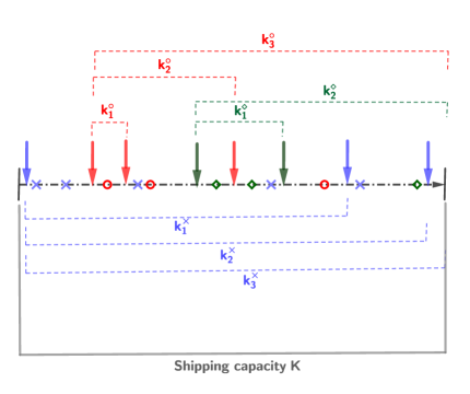
Figure 1: The arrivals of the buyers are indicated by points $\times$(blue), $\circ$(red) and $\diamond$(green) representing different types. Arrows of different colors indicate points in time (beginning of different days in our model) at which the productions of different types happen.

Throughout the paper, we will focus on characterizing the optimal online policy and will evaluate our algorithms against that benchmark. In that sense, we deviate from the prophet inequality framework that compares various policies against the omniscient prophet or equivalently the optimum offline. It is not hard to see, and we will show this later, that these two benchmarks could be off by a factor 2 of each other even for the special case of single item prophet inequality (see also Kleinberg and Weinberg, 2012).

2.2 A simple exponential-sized dynamic program

Our production constrained Bayesian selection problem can be solved exactly using a simple exponential-sized dynamic program. Let $\vec{s}=[s_{1},s_{2},...,s_{m}]\in\mathbb{Z}^{m}$ be the vector maintaining the current number of sold products of different types. We say $\vec{s}$ is a feasible state at time $t$ if it can be reached at time $t$ by a feasible online policy respecting all production constraints and the shipping constraint. It is possible to check whether $\vec{s}$ is feasible at time $t$ using a simple greedy algorithm.

Define $\mathcal{V}_{t}(\vec{s})$ to be the maximum total expected welfare that an online policy can obtain from time $t$ to time $n$ given $\vec{s}$. Define $\mathcal{V}_{t}(\vec{s})=-\infty$ when $s$ is not feasible at time $t$ and $\mathcal{V}_{n+1}(\vec{s})=0$ for all $\vec{s}$. We can compute $\mathcal{V}_{t}(s)$ for the remaining values of $s$ and $t$ recursively as follows. At time $t$, the policy offers the buyer the price $\tau=\tau_{t}(\vec{s})$. Depending on whether or not the value of the customer is above $\tau$, the mechanism obtains either $v_{t}+\mathcal{V}_{t+1}(\vec{s}+\vec{e}_{j_{t}})$ or $\mathcal{V}_{t+1}(\vec{s})$, where $e_{x}$ is the standard basis vector with a single non-zero entry of value $1$ at location $x$ and $j_{t}$ is the request type of buyer $t$. The probability of each event can be computed using the distribution of valuation of buyer $t$. Therefore, the dynamic programming table can be computed using the following rule also known as the Bellman equation:

$$\mathcal{V}_{t}(\vec{s})=\max_{\tau}\left\lparen\mathbb{E}_{#1}[\left\lparen v_{t}+\mathcal{V}_{t+1}(\vec{s}+\vec{e}_{j_{t}})\right\rparen\cdot\mathds{1}[v_{t}\geq\tau]]+\mathbb{E}_{#1}[\mathcal{V}_{t+1}(\vec{s})\cdot\mathds{1}[v_{t}<\tau]]\right\rparen.$$ (1)

Note that the price $\tau_{t}(\vec{s})=\mathcal{V}_{t+1}(\vec{s})-\mathcal{V}_{t+1}(\vec{s}+\vec{e}_{j_{t}})$ maximizes the above equation, and so the final prices of an optimal online policy can be computed easily given the table values.

The above dynamic program has an exponentially large table. In the rest of this section, we describe a linear programming formulation equivalent to the above dynamic program, a natural relaxation for the LP, and a randomized rounding of the relaxation that yields a PTAS.

2.3 Linear programming formulation and ex-ante relaxation

An online policy can be fully described by allocation variables $\mathcal{X}_{t}(\vec{s},v)$, where for every time $t$ and state $\vec{s}$, $\mathcal{X}_{t}(\vec{s},v)$ represents the conditional probability of the event that the buyer at time $t$ is served and the state upon her arrival is $\vec{s}$, conditioned on $v_{t}=v$. We further use state variables $\mathcal{Y}_{t}(\vec{s})$ to represent the probability of the event that an online policy reaches the state $\vec{s}$ upon the arrival of buyer $t$, and auxiliary variables $\mathcal{X}_{t}(v)$ for the marginal allocation probability of buyer $t$ conditioned on $v_{t}=v$.

Having this description, the LP formulation of the dynamic program in Section 2.2 is a combination of two new ideas. The first idea is to ensure the feasibility of the policy by adding the constraint $\mathcal{Y}_{t}(\vec{s})=0$ to the linear program for an infeasible state $\vec{s}$ at time $t$. The second idea is to add another constraint describing how the probability $\mathcal{Y}_{t}(\vec{s})$ updates from time $t$ to $t+1$ as the result of the probabilistic decision made by the policy at time $t$. As will be elaborated more later, this constraint is the necessary and sufficient condition for any policy to be implementable in an online fashion.

Let the set $\mathcal{S}\subset\mathbb{Z}^{m}$ be a finite set containing all possible feasible states at any time $t$. Consider the following exponential-sized (both in the number of variables and constraints) linear program:

$$\begin{array}[]{ll@{}ll}\text{maximize}&\displaystyle\sum_{t=1}^{n}\mathbb{E}_{v_{t}}\left[v_{t}\cdot\mathcal{X}_{t}(v_{t})\right]&\\ \text{subject to}&\{\mathcal{X}_{t}(\vec{s},v),\mathcal{X}_{t}(v),\mathcal{Y}_{t}(\vec{s})\}\in\mathcal{P}^{\textrm{opt}}~{},\end{array}$$ (LP₁)

where $\mathcal{P}^{\textrm{opt}}$ is the polytope of point-wise feasible online policies, defined by these linear constraints:

$$\begin{array}[]{ll@{}ll}&\mathcal{X}_{t}(v)=\displaystyle\sum_{\vec{s}\in\mathcal{S}}\mathcal{X}_{t}(\vec{s},v)&~{}~{}\forall v,~{}t=1,2,\ldots,n,\\ \\ &0\leq\mathcal{X}_{t}(\vec{s},v)\leq\mathcal{Y}_{t}(\vec{s})&~{}~{}\forall v,~{}\vec{s}\in\mathcal{S},t=1,2,\ldots,n,\\ &\mathcal{Y}_{t+1}(\vec{s})=\mathcal{Y}_{t}({\vec{s}})-\mathbb{E}_{v_{t}}\left[\mathcal{X}_{t}(\vec{s},v_{t})\right]+\mathbb{E}_{v_{t}}\left[\mathcal{X}_{t}(\vec{s}-\vec{e}_{j_{t}},v_{t})\right]&~{}~{}\forall\vec{s}\in\mathcal{S},~{}t=1,\ldots,n-1&~{}~{}~{}({\emph{{state update}}})\\ &\mathcal{Y}_{1}(\vec{0})=1\\ &\mathcal{Y}_{t}(\vec{s})=0&~{}~{}\forall\vec{s}\in{\partial\mathcal{S}}(t),t=2,3,\ldots,n.&~{}~{}~{}({\emph{{feasibility check}}})\end{array}$$

where, as a reminder, $j_{t}$ is the type of the buyer arriving at $t$ and $\vec{e}_{x}$ is the standard basis vector with a single non-zero entry of value $1$ at location $x$. We also use $\partial\mathcal{S}(t)$ to denote the set of all forbidden neighboring states at time $t$. It is easy to see that the the set $\partial\mathcal{S}(t)$ has at most $O(n^{K+1})$ states.

$$\partial S(t)\triangleq\left\{\vec{s}\in\mathbb{Z}^{m}:\left[\textrm{$\vec{s}$ is not a feasible state upon the arrival of buyer $t$}\right]~{}\&~{}\left[\exists j~{}\textrm{s.t.}~{}\vec{s}-\vec{e}_{j}\in\mathcal{S}\right]\right\}$$

It is also not hard to see that any feasible online policy induces a feasible assignment for the linear program (LP₁). The only tricky constraint to check is the constraint corresponding to the “state update”. To do so, note that the online policy will reach the state $\vec{s}$ at time $t+1$ if and only if either the state at time $t$ is $\vec{s}$ and the buyer $t$ is not served, or the state at time $t$ is $\vec{s}-\vec{e}_{j_{t}}$ and the buyer $t$ gets served, evolving the state from $\vec{s}-\vec{e}_{j_{t}}$ to $\vec{s}-\vec{e}_{j_{t}}+\vec{e}_{j_{t}}=\vec{s}$.

More importantly, we show the converse holds by proposing an exact rounding algorithm in the form of an adaptive pricing with randomized tie-breaking policy; such a policy offers the price $\tau_{t}(\vec{s})$ to buyer $t$ if the current state is $\vec{s}$. In case of a tie ($v_{t}=\tau_{t}(\vec{s})$), the pricing policy breaks the tie independently with probability $p_{t}(\vec{s})$, in favor of selling the item.

Proposition 2.1.

There exists an adaptive pricing policy with randomized tie breaking, whose expected social-welfare is equal to the optimal solution of the linear program (LP₁) and is a feasible online policy for the production constrained Bayesian selection problem.

We postpone the formal proof and a discussion on how to compute prices and tie-breaking probabilities (given the LP optimal assignment) to Appendix A, and just sketch the main ideas here.

Proof sketch..

Let $\{\mathcal{X}^{*}_{t}(\vec{s},v)\}$ and $\{\mathcal{Y}^{*}_{t}(\vec{s})\}$ be the optimal solutions of LP₁. Consider the following simple online randomized rounding scheme: start from the all-zero assignment at time $t<1$. Now, suppose at time $t\geq 1$, the current state, i.e., number of sold products of different types, is $\vec{s}$ and the realized buyer value is $v_{t}=v$. The rounding algorithm first checks whether $\mathcal{Y}^{*}_{t}(\vec{s})$ is zero. If yes, it skips the buy request. Otherwise, it accepts the request with probability $\tfrac{\mathcal{X}^{*}_{t}(\vec{s},v)}{\mathcal{Y}^{*}_{t}(\vec{s})}$.

It is not hard to show this simple scheme will have allocation and state probabilities matching the LP optimal assignment, i.e. $\{\mathcal{X}^{*}_{t}(\vec{s},v)\}$ and $\{\mathcal{Y}^{*}_{t}(\vec{s})\}$. Moreover, $\mathcal{Y}^{*}_{t}(\vec{s})=0$ for all forbidden neighboring states $\vec{s}$, i.e. infeasible states that can only be reached from a feasible state at time $t$ by accepting an extra request. Hence an inductive argument shows that the resulting online policy is always feasible. There is also a simple coupling argument, with shifting the probability masses to higher values, showing that the above algorithm can be implemented using an adaptive pricing policy with the randomized tie breaking. Prices and probabilities can then be computed by straightforward calculations. ∎

Ex-ante relaxation.

LP₁ has exponential size. Nevertheless, without a shipping constraint, it can be solved in polynomial time. In fact, any online policy can be decomposed into $m$ separate online policies for type-specific sub-problems; in each sub-problem, its corresponding policy only requires to respect the production constraints of its type. At the same time, the dynamic programming table of each sub-problem $j$ is polynomial-sized, as the state at time $t$ is essentially the number of sold products of type $j$ before $t$. Therefore the overall optimal online policy can be computed in polynomial time.

What if we relax the shipping constraint to hold only in expectation (over the randomness of the policy/values)? This relaxation is used in the prophet inequality literature (Alaei et al., 2015; Feldman et al., 2016; Düetting et al., 2017; Lee and Singla, 2018), where is termed as the ex-ante relaxation.

Similar to the linear program of the optimal online policy (LP₁), we formulate the ex-ante relaxation as an LP. First, re-define $\mathcal{S}\triangleq[1:{\max}_{j}~{}{k^{j}_{T}}]$ to be the set of possible states of each sub-problem. Second, for each type $j$ and buyer $t\in B^{j}$, we use allocation variables $\mathcal{X}_{t}(s_{j},v)$, marginal variables $\mathcal{X}_{t}(v)$, and state variables $\mathcal{Y}_{t}(s_{j})$, where $s_{j}$ represents the number of sold items of type $j$ before the arrival of buyer $t$. We further use variables ${\mathcal{N}}_{j}$ to represent the expected number of served buyers of each type $j$.

$$\begin{array}[]{ll@{}ll}\text{maximize}&\displaystyle\sum_{t=1}^{n}\mathbb{E}_{v_{t}}\left[v_{t}\cdot\mathcal{X}_{t}(v_{t})\right]&&\\ \text{subject to}&\displaystyle\sum_{t\in B^{j}}\mathbb{E}_{v_{t}}\left[\mathcal{X}_{t}(v_{t})\right]\leq{\mathcal{N}}_{j},&~{}~{}~{}j=1,\ldots,m.\\ &\{\mathcal{X}_{t}(s_{j},v),\mathcal{X}_{t}(v),\mathcal{Y}_{t}(s_{j})\}_{t\in B^{j}}\in\mathcal{P}^{\textrm{sub}_{j}},&~{}~{}~{}j=1,\ldots,m.\\ &\displaystyle\sum_{j=1}^{m}{\mathcal{N}}_{j}\leq K.&~{}~{}~{}\emph{(shipping capacity in expectation)}\end{array}$$ (LP₂)

where $B^{j}\subseteq[n]$ is the set of all buyers of type $j$ and $\mathcal{P}^{\textrm{sub}_{j}}$ is the polytope of point-wise feasible online policies for serving type $j$ buyers, defined by the following set of linear constraints (similar to LP₁):

$$\begin{array}[]{ll@{}ll}&\mathcal{X}_{t}(v)=\displaystyle\sum_{s_{j}\in\mathcal{S}}\mathcal{X}_{t}(s_{j},v)&~{}~{}\forall v,~{}t\in B^{j},\\ \\ &0\leq\mathcal{X}_{t}(s_{j},v)\leq\mathcal{Y}_{t}(s_{j})&~{}~{}\forall v,~{}s_{j}\in\mathcal{S},t\in B^{j},\\ &\mathcal{Y}_{t}(s_{j})=\mathcal{Y}_{t^{\prime}}(s_{j})-\mathbb{E}_{v_{t^{\prime}}}\left[\mathcal{X}_{t^{\prime}}(s_{j},v_{t^{\prime}})\right]+\mathbb{E}_{v_{t^{\prime}}}\left[\mathcal{X}_{t^{\prime}}(s_{j}-1,v_{t^{\prime}})\right]&~{}~{}\forall s_{j}\in\mathcal{S},~{}t,t^{\prime}\in B^{j},~{}~{}~{}~{}~{}({\emph{{state update}}})\\ &&~{}~{}[t^{\prime}+1:t-1]\cap B^{j}=\emptyset\\ \\ &\mathcal{Y}_{t_{0}}(0)=1&~{}~{}t_{0}=\min\{t\in B^{j}\}\\ &\mathcal{Y}_{t}(s_{j})=0&~{}~{}\forall s_{j}\in\partial\mathcal{S}^{j}(t),t\in B^{j}.~{}~{}~{}~{}({\emph{{feasibility check}}})\end{array}$$

where $\partial\mathcal{S}(t)$ is the set of all forbidden neighboring states of the sub-problem of type $j$ at time $t$, i.e.

$$\partial S^{j}(t)\triangleq\left\{s\in\mathbb{Z}:\left[\textrm{${s}$ is greater than the total production of type $j$ up to time $t$}\right]~{}\&~{}\left[s\leq\underset{j}{\max}~{}k_{T}^{j}+1\right]\right\}$$

Note that because of the collapse of the state space, LP₂ program has polynomial size.

As every online policy for our problem induces a feasible online policy for each request type $j$, and because it respects the shipping capacity point-wise, we have the following proposition.

Proposition 2.2.

LP₂ is a relaxation of the optimal online policy for maximizing expected social-welfare in the production constrained Bayesian selection problem.

2.4 Polynomial-Time Approximation Scheme (PTAS)

Given parameter $\epsilon>0$, our proposed polynomial time approximation scheme is based on solving a linear program with size polynomial in $n$ and an adaptive pricing mechanism with randomized tie breaking that rounds this LP solution to a $\left(1-O(\epsilon)\right)$-approximation. For notation purposes here and in Section 2.5, let $\{\mathcal{X}^{*}_{t}(\vec{s},v_{t}),\mathcal{X}^{*}_{t}(v_{t}),\mathcal{Y}^{*}_{t}(\vec{s})\}$ be the optimal assignment of LP₁, and $\{\mathcal{X}^{*}_{t}(s_{j},v_{t}),\mathcal{X}^{*}_{t}(v_{t}),\mathcal{Y}^{*}_{t}(s_{j}),{\mathcal{N}}^{*}_{j}\}$ be the optimal assignment of LP₂ for the buyers $t\in B^{j}$.

Overview.

Consider the linear program of the optimal online policy (LP₁) and the ex-ante relaxation (LP₂). For a given constant $\delta>0$, we turn to one of these linear programs, depending on whether the shipping capacity $K$ is small ($K\leq\frac{1}{\delta}$) or large ($K>\frac{1}{\delta}$). In the former case, we pay the computational cost of solving LP₁ and then round it exactly to a point-wise feasible online policy. In the latter case, we first reduce the large shipping capacity $K$ by a factor of $(1-\epsilon)$ to create some slack, and then solve LP₂ with this reduced shipping capacity (which has polynomial size). We then round the LP solution exactly by an adaptive pricing with randomized tie breaking policy. The hope is the resulting online policy respects all the constraints of the production constrained Bayesian selection problem with high probability because:

1. For every type $j$, the policy respects the corresponding production constraints point-wise.

2. The policy respects the reduced large shipping capacity in expectation.

3. Moreover, we show that the total number of served buyers concentrates because of the negative dependency of the selection rule.

4. Finally, due to the available slack in the large shipping capacity and because of the mentioned concentration, this capacity is exhausted with small probability.

The algorithm.

More precisely, we run the following algorithm (Algorithm 1).

Algorithm 1 PTAS-Production-Constrained ($\epsilon,\delta$)

1:Input parameters $\epsilon,\delta>0$.

2:if $\left(K\leq\frac{1}{\delta}~{}\textrm{i.e. when shipping capacity is small}\right)$ then

3:    Solve the linear program of optimal online policy (LP₁).

4:    Given the optimal assignment, extract adaptive prices $\tau_{t}(\vec{s})$ and tie-breaking probabilities $\tau_{t}(\vec{s})~{},\forall\vec{s}\in\mathcal{S}$.

5:else $\left(K>\frac{1}{\delta}~{}\textrm{i.e. when shipping capacity is large}\right)$

6:    Reduce the shipping capacity $K$ by a multiplicative factor $(1-\epsilon)$.

7:    Solve the ex-ante relaxation linear program (LP₂) with the reduced shipping capacity of $K(1-\epsilon)$.

8:    for product types $j=1,2,\ldots,m$ do

9:         Given the optimal assignment corresponding to the variables of type $j$, extract adaptive prices $\tau_{t}(s_{j})$           and tie-breaking probabilities $p_{t}(s_{j})$ for every $s_{j}\in\mathcal{S}$ and every buyer $t$ such that $j_{t}=j$.

10:    end for

11:end if

12:Offer the adaptive prices (with randomized tie breaking) computed above to arriving buyers based on their types $j$. In the exceptional cases when there is no remaining shipping capacity, offer the price of infinity.

Computing prices and tie-breaking probabilities.

Given $\{\mathcal{X}^{*}_{t}(\vec{s},v_{t}),\mathcal{Y}^{*}_{t}(\vec{s})\}$, the proof of Proposition 2.1 in Appendix A (sketched in Section 2.3) gives a recipe to find $\tau_{t}(\vec{s})$ and $p_{t}(\vec{s})$ efficiently, so that the corresponding adaptive pricing with randomized tie-breaking policy maintains the same expected marginal allocation $\mathbb{E}_{v_{t}}\left[\mathcal{X}^{*}_{t}(\vec{s},v_{t})\right]$ as the optimal online policy for every buyer $t$ and state $\vec{s}\in\mathcal{S}$, while having at least the same expected social-welfare.

For the case of large shipping capacity, we apply exactly the same argument for each sub-problem $j$ separately. Given $\{\mathcal{X}^{*}_{t}(s_{j},v_{t}),\mathcal{Y}^{*}_{t}(s_{j}),{\mathcal{N}}^{*}_{j}\}$ for ${t\in B^{j}}$, we can efficiently find prices $\tau_{t}(s_{j})$ and probabilities $p_{t}(s_{j})$, so that the corresponding adaptive pricing with randomized tie-breaking for buyers with type $j$ maintains the same expected marginal allocation $\mathbb{E}_{v_{t}}\left[\mathcal{X}^{*}_{t}(s_{j},v_{t})\right]$ for every $t\in B^{j}$ and $s_{j}\in\mathcal{S}$, while having at least the same expected social-welfare from serving each individual buyer of type $j$.

Feasibility, running time and social-welfare.

Clearly, Algorithm 1 is a feasible online policy in the case of small shipping capacity (Proposition 2.1). In the case of large shipping capacity, as $\mathcal{Y}^{*}_{t}(s_{j})=0$ for any forbidden neighboring state of sup-problem $j$, the same argument shows that it respects all of the production constraints of each type $j$. The policy also never violates the shipping capacity by construction, and hence is feasible. In terms of running time, the linear program of optimal online policy LP₁ has at most $n^{\frac{1}{\delta}}$ states, as no more than $\frac{1}{\delta}$ requests can be accepted. By setting $\delta=\epsilon^{2}/\log(1/\epsilon)$, Algorithm 1 has running time $\texttt{poly}(n^{\frac{\log(1/\epsilon)}{\epsilon^{2}}})$. We further show that its expected welfare is at least $(1-O(\epsilon))$ fraction of the expected welfare of the optimal online policy (whose proof is deferred to Section 2.4.1, Proposition 2.6).

Theorem 2.3 (PTAS for optimal online policy).

By setting $\delta=\frac{\epsilon^{2}}{\log(1/\epsilon)}$, Algorithm 1 is a $(1-O(\epsilon))$-approximation for the expected social-welfare of the optimal online policy of the production constrained Bayesian selection problem, and runs in time $\texttt{poly}(n^{\frac{\log(1/\epsilon)}{\epsilon^{2}}})$.

Corollary 2.4 (PTAS to maximize revenue).

By applying Myerson’s lemma from Bayesian mechanism design (Hartline, 2012; Myerson, 1981) and replacing each buyer value $v_{t}$ with her ironed virtual value $\bar{\phi}_{t}(v_{t})$, Theorem 2.3 gives a PTAS for the optimal online policy for maximizing expected-revenue.

2.4.1 Analysis of the algorithm (proof of Theorem 2.3)

If the shipping capacity is small, i.e. $K\leq\frac{1}{\delta}$, Algorithm 1 has the optimal expected social-welfare among all the feasible online policies, because of the optimality of LP₁ (Proposition 2.1). Next consider the ex-ante relaxation LP in the case when $K>\frac{1}{\delta}$. By Proposition 2.2, its optimal solution is an upper bound on the social-welfare of any feasible online policy. By scaling the shipping capacity by a factor $(1-\epsilon)$, we change the optimal value of this LP by only a multiplicative factor of at least $(1-\epsilon)$.

As sketched before, for each type $j$ the adaptive pricing policies $\{\tau_{t}(s_{j}),p_{t}(s_{j})\}$ extract an expected value from buyer $t$ that is at least equal to the contribution of this buyer to the objective value of the ex-ante relaxation LP. However, buyer $t$ can be served by the adaptive pricing policy of type $j_{t}$ only if the large shipping capacity has not been exceeded yet. So, to bound the loss, the only thing left to prove is that the probability of this bad event is small (as small as $O(\epsilon)$).

Concentration and negative cylinder dependency.

In the case when the shipping capacity is large, let $X_{t}\in\{0,1\}$ be a Bernoulli random variable, indicating whether the resulting pricing policy of type $j_{t}$ serves the buyer $t$ or not. Note that $\sum_{t}\mathbb{E}[X_{t}]\leq(1-\epsilon)K$, as LP₂ ensures feasibility of the shipping constraint in expectation. Now, if the total count $\sum_{t}X_{t}$ concentrates around its expectation, we will be able to bound the probability of the bad event that the shipping capacity is exceeded.

Clearly, $\{X_{t}\}_{t\in B^{1}},\{X_{t}\}_{t\in B^{2}},\ldots,\{X_{t}\}_{t\in B^{m}}$ are mutually independent, as we run a separate adaptive pricing policy for each type $j$. However, the indicators random variables of the same type are not mutually independent with each other. So, for proving the required concentration, Chernoff bound cannot be applied immediately. Yet, we can use a certain variant of negative dependency instead of independence (Dubhashi and Ranjan, 1998; Pemantle, 2000; Chekuri et al., 2009), known as the negative cylinder dependency, and still prove Chernoff-style concentration bounds.

Definition 2.5 (Negative cylinder dependency, Pemantle (2000)).

Random variables $X_{1},...,X_{n}$ satisfy the negative cylinder property if and only if for every $S\subseteq[1:n]$,

$$\mathbb{E}[\displaystyle\prod_{t\in S}X_{t}]\leq\displaystyle\prod_{t\in S}\mathbb{E}[X_{t}]$$ (2)

We now prove the following proposition, assuming the required negative cylinder dependency.

Proposition 2.6.

If for every request type $j$, the random variables $\{X_{t}\}_{t\in B^{j}}$ satisfy the negative cylinder dependency and if $K>\frac{1}{\delta}=\frac{\log(1/\epsilon)}{\epsilon^{2}}$, then the probability that the shipping capacity $K$ is exhausted is $O(\epsilon)$.

Proof.

Applying the negative cylinder dependency property, for every $\alpha>0$ we have:

$$\mathbb{E}[\displaystyle\prod_{t}e^{\alpha X_{t}}]=\mathbb{E}[\displaystyle\prod_{j\in[m]}\prod_{t\in B^{j}}\left(1+(e^{\alpha}-1)\cdot X_{t}\right)]\overset{(1)}{\leq}\displaystyle\prod_{t}\left(1+(e^{\alpha}-1)\cdot\mathbb{E}[X_{t}]\right)=\displaystyle\prod_{t}\mathbb{E}[e^{\alpha X_{t}}],$$ (3)

where in (1) we use the negative cylinder property among $\{X_{t}\}_{t\in B^{j}}$ for each type $j$, and the mutual independence of the Bernoulli variables across different types. Now, as Eq. 3 is essentially the first step of the proof of Chernoff bound, it ensures that we have a Chernoff-type concentration (Dubhashi and Ranjan, 1998). Therefore, as $\sum_{t}\mathbb{E}[X_{t}]\leq(1-\epsilon)K$, we have:

$$\mathbb{P}[\displaystyle\sum_{t}X_{t}>K]\leq\mathbb{P}[\displaystyle\sum_{t}(X_{t}-\mathbb{E}[X_{t}])>\epsilon K]\leq e^{-\frac{K\epsilon^{2}}{3}}=O(\epsilon). \square$$

∎

2.5 Negative cylinder dependency for optimal online policy

Fix a product type $j$. For notation simplicity, re-index $\{X_{t}\}_{t\in B^{j}}$ as $X_{t_{1}},\ldots,X_{t_{l}}$, where $t_{1}\leq t_{2}\leq\ldots\leq t_{l}$ and $l\triangleq\lvert B^{j}\rvert$. To show $\{X_{t_{i}}\}$ satisfy the negative cylinder dependency, it is enough to show that:

$$\forall i\in[1:l],S\subseteq[1:l]:\mathbb{P}[X_{t_{i}}=1\nonscript\>|\nonscript\>\mathopen{}\displaystyle\bigcap_{i^{\prime}\in S}\{X_{t_{i^{\prime}}}=1\}]\leq\mathbb{P}[X_{t_{i}}=1]$$ (4)

To see this, note that $X_{t}\in\{0,1\}$. Hence if Eq. 4 holds, we have

$$\mathbb{E}[\displaystyle\prod_{i=1}^{l}X_{t_{i}}]=\mathbb{P}[\displaystyle\bigcap_{i=1}^{l}\{X_{t_{i}}=1\}]=\displaystyle\prod_{i=1}^{l}\mathbb{P}[X_{t_{i}}=1|\bigcap_{j\leq i-1}\{X_{t_{j}}=1\}]\overset{\lx@cref{creftype~refnum}{eq:neg-alter}}{\leq}\displaystyle\prod_{i=1}^{l}\mathbb{P}[X_{t_{i}}=1]=\displaystyle\prod_{i=1}^{l}\mathbb{E}[X_{t_{i}}]$$

which shows the negative cylinder dependence. Given this simple observation, one needs to show that for the adaptive pricing with randomized tie-breaking used in Algorithm 1, the probability of accepting a buy request at time $t$ can only decrease conditioned on more requests being accepted in the past. Another neat observation is that given ${\mathcal{N}}^{*}_{j}$ as the optimal soft shipping capacity that needs to hold only in expectation, $\{\mathcal{X}^{*}_{t}(s_{j},v_{t}),\mathcal{X}^{*}_{t}(v_{t}),\mathcal{Y}^{*}_{t}(s_{j})\}$ for $t\in B^{j}$ is indeed the optimal solution of the following linear program.

$$\begin{array}[]{ll@{}ll}\text{maximize}&\displaystyle\sum_{t\in B^{j}}\mathbb{E}_{v_{t}}\left[v_{t}\cdot\mathcal{X}_{t}(v_{t})\right]&&\\ \text{subject to}&\displaystyle\sum_{t\in B^{j}}\mathbb{E}_{v_{t}}\left[\mathcal{X}_{t}(v_{t})\right]={\mathcal{N}}^{*}_{j},&~{}~{}~{}\emph{(soft shipping constraint)}\\ &\{\mathcal{X}_{t}(s_{j},v),\mathcal{X}_{t}(v),\mathcal{Y}_{t}(s_{j})\}_{t\in B^{j}}\in\mathcal{P}^{\textrm{sub}_{j}}.&\end{array}$$ (LP-sub_j)

Therefore, it is enough to show the same property holds for another adaptive pricing with randomized tie-breaking algorithm that is used for exactly rounding LP-sub_j, as both of these rounding algorithms have the same allocation distribution for the buyers of type $j$.

For simplicity of the proofs in this section, we assume that the valuations are non-atomic. Note that under this assumption, there will be no need for randomized tie breaking, and indeed our rounding algorithm will be a pure adaptive pricing. We now prove our claim in two steps.

1. Step 1: by using LP duality, we show that the optimal online policy of the sub-problem of type $j$ with an extra soft shipping constraint ${\mathcal{N}}^{*}_{j}$ is indeed the optimal online policy for an instance that has no soft constraint and all the values are shifted by some number $\lambda^{*}$, i.e. $\hat{v}_{t}=v_{t}-\lambda^{*}$.

2. Step 2: we show that the optimal online policy of a particular sub-problem $j$, whether value distributions have negative points in their support or not, satisfies the negative cylinder dependency.

Putting the two pieces, we prove the negative cylinder dependency among $X_{t_{1}},...,X_{t_{l}}$ as desired. In the remaining of this section, we prove the two steps.

Proof of Step 1.

Consider (LP-sub_j) that captures the optimal online policy of sub-problem $j$. We start by moving the soft shipping constraint into the objective of of (LP-sub_j) and writing the Lagrangian.

$$\begin{array}[]{ll@{}ll}\underset{\lambda}{\text{minimize}}~{}\underset{\mathcal{X}}{\text{maximize}}&\displaystyle\mathcal{L}(\mathcal{X},\lambda)=\sum_{t\in B^{j}}\mathbb{E}_{v_{t}}\left[v_{t}\cdot\mathcal{X}_{t}(v_{t})\right]+\lambda({\mathcal{N}}_{j}^{*}-\sum_{t\in B^{j}}\mathbb{E}_{v_{t}}\left[\mathcal{X}_{t}(v_{t})\right])&\\ &\{\mathcal{X}_{t}(s_{j},v),\mathcal{X}_{t}(v),\mathcal{Y}_{t}(s_{j})\}_{t\in B^{j}}\in\mathcal{P}^{\textrm{sub}_{j}}.&\end{array}$$

Let $\lambda^{*}$ be the optimum dual solution. By dropping the constant terms and rearranging we get the following equivalent program for the optimal solution:

$$\begin{array}[]{ll@{}ll}{\text{maximize}}&\displaystyle\sum_{t\in B^{j}}\mathbb{E}_{v_{t}}\left[(v_{t}-\lambda^{*})\cdot\mathcal{X}_{t}(v_{t})\right]\\ &\{\mathcal{X}_{t}(s_{j},v),\mathcal{X}_{t}(v),\mathcal{Y}_{t}(s_{j})\}_{t\in B^{j}}\in\mathcal{P}^{\textrm{sub}_{j}}.&\end{array}$$

This shows that the optimal online policy respecting the soft shipping constraint ${\mathcal{N}}_{j}^{*}$ is equivalent to the optimal online policy for an instance of the problem where all the values are shifted by some constant $\lambda^{*}$. ∎

Proof of Step 2.

We only need to show that the negative cylinder dependency holds for the dynamic programming that solves each sub-problem, as the distributions are non-atomic and there is a unique deterministic optimal online policy, characterized both by the LP and the dynamic programming. Consider sub-problem $j$. We use induction to show by serving more customers in the past, the prices for new buyers increase. Let $s_{t}^{j}$ denote the total number of products of type $j$ that have been sold up to the arrival of buyer $t$. Note that the algorithm only needs $s_{t}^{j}$ to decide whether buyer $t$ should be served.

Let $D_{t}(s_{t}^{j})$ denote the maximum total expected welfare that an online policy can obtain from time $t$ to $n$, assuming that it starts from state $s_{t}^{j}$. Also let $C_{t}^{j}$ denote the set of production checkpoints of type $j$ that occur at or after time $t$. Using the Bellman equations we have

$$D_{t-1}(s_{t-1}^{j})=\left\{\begin{array}[]{@{}l@{\thinspace}l}D_{t}(s_{t-1}^{j})&~{}~{}\textrm{if}~{}~{}\min\left(\left\{k_{i}^{j}-s_{t-1}^{j}\right\}_{i\in C_{t-1}^{j}}\right)=0\\ \mathbb{E}_{v_{t-1}}\left[\max(D_{t}(s_{t-1}^{j}+1)+v_{t-1},D_{t}(s_{t-1}^{j}))\right]&~{}~{}\textrm{if}~{}~{}\min\left(\left\{k_{i}^{j}-s_{t-1}^{j}\right\}_{i\in C_{t-1}^{j}}\right)>0\\ \end{array}\right.$$

As the base of our induction, we know that if we serve the last buyer, the probability that we serve any other buyers does not increase. Now assume while serving buyer $t$, we have

$$D_{t}(s_{t}^{j})-D_{t}(s_{t}^{j}+1)\leq D_{t}(s_{t}^{j}+1)-D_{t}(s_{t}^{j}+2).$$ (5)

Note that this shows the price offered to buyer $t$ increases if we serve more buyers before buyer $t$. When buyer $t-1$ arrives, we need to show

$$D_{t-1}(s_{t-1}^{j})-D_{t-1}(s_{t-1}^{j}+1)\leq D_{t-1}(s_{t-1}^{j}+1)-D_{t-1}(s_{t-1}^{j}+2)$$ (6)

which is equivalent to

$$D_{t-1}(s_{t-1}^{j})+D_{t-1}(s_{t-1}^{j}+2)\leq 2D_{t-1}(s_{t-1}^{j}+1).$$

Note that this property is linear in the terms involved. So it is enough to assume that the value $v_{t-1}$ is deterministic first and prove the above inequality. Then by linearity of expectation, the inequality would hold in the general case.

Note that for the case where $\min\left(\left\{k_{i}^{j}-s_{t-1}^{j}\right\}_{i\in C_{t-1}^{j}}\right)<2$, the inequality holds trivially because we assume $D_{t-1}(s)=-\infty$ for any non-negative integer $s$ such that $\min\left(\left\{k_{i}^{j}-s\right\}_{i\in C_{t-1}^{j}}\right)<0$. According to our induction hypothesis, if $D_{t-1}(s_{t-1}^{j}+2)$ is updated, then the other two variables are updated as well. More precisely, if $D_{t-1}(s_{t-1}^{j}+2)=D_{t}(s_{t-1}^{j}+3)+v_{t-1}$, then

$$D_{t-1}(s_{t-1}^{j}+1)=D_{t}(s_{t-1}^{j}+2)+v_{t-1},$$

$$D_{t-1}(s_{t-1}^{j})=D_{t}(s_{t-1}^{j}+1)+v_{t-1}.$$

In a similar way, if $D_{t-1}(s_{t-1}^{j}+1)=D_{t}(s_{t-1}^{j}+2)+v_{t-1}$, then

$$D_{t-1}(s_{t-1}^{j})=D_{t}(s_{t-1}^{j}+1)+v_{t-1}.$$

Considering these relations, we have three different cases. (i) none of these variables are updated. In this case, Eq. 6 turns into Eq. 5 which holds according to our induction hypothesis. (ii) all of these variables are updated. In this case, Eq. 6 turns into

$$D_{t}(s_{t}^{j}+1)+v_{t-1}-D_{t}(s_{t}^{j}+2)-v_{t-1}\leq D_{t}(s_{t}^{j}+2)+v_{t-1}-D_{t}(s_{t}^{j}+3)-v_{t-1}$$

which holds again according to the induction hypothesis. Finally, (iii) the case where $D_{t-1}(s_{t-1}^{j})$ is updated and $D_{t-1}(s_{t-1}^{j}+2)$ is not updated. In this case, we can write Eq. 6 as

$$D_{t}(s_{t}^{j}+1)+v_{t-1}+D_{t}(s_{t}^{j}+2)\leq 2\max(D_{t}(s_{t}^{j}+2)+v_{t-1},D_{t}(s_{t}^{j}+1))$$

and this always holds because for any two values $x,y$, $\frac{x+y}{2}\leq\max(x,y)$. ∎

3 Generalization to the Laminar Matroid Bayesian Selection

Another approach to the production constrained Bayesian selection problem is to view it as follows: for each product type $j$, nested subsets $B_{1}^{j}\subseteq\ldots\subseteq B_{T}^{j}\subseteq B^{0}\triangleq[n]$ are given, where $B^{0}$ has capacity $K$ and each subset $B_{i}^{j}$ has capacity $k_{i}^{j}$. A subset of requests in $[n]$ is considered to be feasible if from each subset $B^{0}$ or $B_{i}^{j}$ no more than their capacities are selected. This alternative view suggests looking at the problem as a special case of a combinatorially richer stochastic online optimization problem known as the laminar matroid Bayesian selection (Kleinberg and Weinberg, 2012; Feldman et al., 2016).

3.1 Problem description

In a laminar matroid Bayesian selection problem, we have a set of $n$ elements and a laminar family of subsets of these elements termed as the bins, i.e. a collection $\mathscr{F}$ of subsets where for every $B,B^{\prime}\in\mathscr{F}$ either $B\subseteq B^{\prime}$, $B^{\prime}\subseteq B$ or $B\cap B^{\prime}=\emptyset$. It is often helpful to represent the laminar family as a tree whose internal nodes are the bins and the leaves are the elements. The elements arrive over time in an arbitrary but known order, and reveal their values. We further assume values are drawn independently from known heterogeneous distributions. Moreover, each bin $B$ has capacity $k_{B}$. The goal is to design an online policy/algorithm for selecting a subset of elements $1,2,\cdots,n$ with maximum possible total expected value, so that no more than $k_{B}$ elements are picked from each bin $B$. Figure 2 describes how this problem generalizes the production constrained Bayesian selection problem of Section 2.

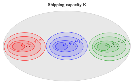
Figure 2: Production constrained Bayesian selection as a special case of Laminar Bayesian selection; each of the types $\circ$(red), $\times$(blue), and $\diamond$(green) has a corresponding collection of nested bins (path laminar), and these bins are inside an outer bin $[n]$ to model the shipping constraint.

We consider generalizing the machinery developed in Section 2 to this problem. Again, similar to Section 2, we deviate from the prophet inequality framework that compares various policies against the omniscient prophet or equivalently the optimum offline. Our main result in this section is a PTAS for the optimal online policy, when the depth of the family (or equivalently the height of the tree) is constant. We also show that our final algorithm has the form of an adaptive pricing with randomized tie-breaking.

We further generalize our setting by replacing each singleton element with a laminar Bayesian selection sub-problem. As a simple corollary, we show our result holds if the optimal online policy for each sub-problem can be implemented efficiently and satisfies the negative cylinder dependency (Definition 2.5). Notably, the production constrained Bayesian selection is subsumed under this corollary as a special case.

3.2 Sketch of our approach

Our general strategy to solve this problem is to first divide the internal nodes of the laminar tree into large and small bins, similar to what we did for the shipping constraint in the previous section. To do so, we start from the root, and mark each node as either large or small. Once a bin is marked as small, all of its descendants will also be marked as small. Next, inspired by our approach in Section 2, we proceed with these steps:

1. Finding a linear programming formulation for characterizing feasible online policies in each small bin. As in Section 2, we use an state update rule (similar to the dynamic programming update) to help us with this characterization.

2. Writing a hierarchy of linear programming relaxations, where the relaxations are parameterized by how we divide the bins into small and large. For a given marking, the corresponding relaxation should select a point-wise feasible online policy in each small bin, and impose global capacity constraints that hold only in expectation for large bins.

3. Using a particular marking algorithm to select a polynomially solvable linear programming relaxation in the above mentioned hierarchy.

4. Using an adaptive pricing with randomized tie-breaking to round this LP relaxation.

5. Using a concentration argument to show large capacities are only violated with small probabilities.

We next elaborate more on each of the bullets above, while highlighting the new technical pieces we need to add to the techniques in Section 2.

3.3 A hierarchy of linear programming relaxations for general laminar matroids

We define a family of linear programming relaxations, parametrized by different markings of bins into small and large. Given a particular marking, as described in Section 3.2, let $\mathscr{L}$ be the set of large bins and $\mathscr{S}$ be the set of maximal small bins.

For an instance of the laminar matroid Bayesian selection problem with laminar family $\mathscr{F}$, an online policy is said to be at the state $\vec{s}\in\mathbb{Z}^{\mathscr{F}}$ upon the arrival of an element if $\vec{s}$ is the vector of remaining capacities of all of the bins in $\mathscr{F}$. Given this definition, the state $\vec{s}$ is a sufficient information to find the optimal online policy from time $t$ to $n$, for both the allocation and the expected social-welfare, using (an exponential-time) dynamic programming à la Section 2.2.

To avoid exponentially many states in our hierarchy of LP relaxations, we use the same state-space structure, but we only track the local state of each maximal small bin in $\mathscr{S}$ separately. In other words, we can think of each maximal small bin $B$ as a separate laminar matroid Bayesian selection sub-problem with laminar family $\mathscr{F}^{B}\triangleq\{B^{\prime}\in\mathscr{F}:B^{\prime}\subseteq B\}$, where each arriving element is only in one of the sub-problems (because subsets in $\mathscr{S}$ form a partition of the set of all elements). Now, if the arriving element at time $t$ belongs to $B\in\mathscr{S}$, the linear program only needs to keep track of the change in the local state $\vec{s}\in\mathbb{Z}^{\mathscr{F}^{B}}$ of the sub-problem $B$, i.e. the vector of remaining capacities of the bins in $\mathscr{F}^{B}$.

For every small bin $B$, define $\mathcal{S}^{B}$ to be the set of all feasible local states of the sub-problem $B$, i.e. the set of all possible remaining capacity vectors of the bins in $\mathscr{F}^{B}$, where each vector can be reached by an online policy for this sub-problem that respects all the capacities in $\mathscr{F}^{B}$ . Note that $\lvert\mathcal{S}^{B}\rvert\leq n^{k_{B}}$, because no feasible online policy for the sub-problem $B$ can pick more than $k_{B}$ elements. We now can write a linear program with the following variables and constraints:

Variables.

We add allocation variables $\mathcal{X}_{t}(\vec{s},v)$, marginal allocation variables $\mathcal{X}_{t}(v)$ and state variables $\mathcal{Y}_{t}(\vec{s})$ as before, in a similar fashion to the ex-ante relaxation linear program (LP₂) in Section 2. For the variables $\mathcal{X}_{t}(\vec{s},v)$ and $\mathcal{Y}_{t}(\vec{s})$, assuming the element arriving at time $t$ belongs to the maximal small bin $B$, the vector $\vec{s}$ represents the local state of $B$ right before arrival of this element.

Constraints.

We add two categories of linear constraints to our LP relaxations:

• Global ex-ante constraints: these constraints ensure that the capacity of all large bins are respected in expectation, i.e.

  $$\forall B\in\mathscr{L}:\displaystyle\sum_{t\in B}\mathbb{E}_{v_{t}}\left[\mathcal{X}_{t}(v_{t})\right]\leq k_{B}$$

• Local online feasibility constraints: for every bin $B\in\mathscr{S}$, similar to LP₂, we can define a polytope $\mathcal{P}^{B}$ of feasible online policies that ensures a feasible assignment of the linear program is online implementable by a feasible policy. So, these constraints will be:

  $$\forall B\in\mathscr{S}:\{\mathcal{X}_{t}(\vec{s},v),\mathcal{X}_{t}(v),\mathcal{Y}_{t}(\vec{s})\}\in\mathcal{P}^{B}$$

Polytope of feasible online policies.

The polytope $\mathcal{P}^{B}$ is defined using exactly the same style of linear constraints as in $\mathcal{P}^{\textrm{sub}_{j}}$ (Section 2.3, LP₂), with some slight modifications:

$$\begin{array}[]{ll@{}ll}&\mathcal{X}_{t}(v)=\displaystyle\sum_{\vec{s}\in\mathcal{S}^{B}}\mathcal{X}_{t}(\vec{s},v)&~{}~{}~{}~{}\forall v,~{}t\in B,\\ \\ &0\leq\mathcal{X}_{t}(\vec{s},v)\leq\mathcal{Y}_{t}(\vec{s})&~{}~{}~{}~{}\forall v,~{}\vec{s}\in\mathcal{S}^{B},t\in B,\\ &\mathcal{Y}_{t}(\vec{s})=\mathcal{Y}_{t^{\prime}}({\vec{s}})-\mathbb{E}_{v_{t^{\prime}}}\left[\mathcal{X}_{t^{\prime}}(\vec{s},v_{t^{\prime}})\right]+\mathbb{E}_{v_{t^{\prime}}}\left[\mathcal{X}_{t^{\prime}}(\vec{s}+\vec{d}_{t^{\prime}},v_{t^{\prime}})\right]&~{}~{}~{}~{}\forall\vec{s}\in\mathcal{S}^{B},~{}t,t^{\prime}\in B,~{}~{}~{}~{}~{}({\emph{{Bellman eq.}}})\\ &&~{}~{}~{}~{}[t^{\prime}+1:t-1]\cap B=\emptyset\\ \\ &\mathcal{Y}_{t_{0}}([k_{B^{\prime}}]_{B^{\prime}\in\mathscr{F}^{B}})=1&~{}~{}~{}~{}t_{0}=\min\{t\in B\}\\ &\mathcal{Y}_{t}(\vec{s})=0&~{}~{}~{}~{}\forall\vec{s}\in\partial\mathcal{S}^{B},t\in B.\end{array}$$

where $\vec{d}_{t}\in\{0,1\}^{\mathscr{F}^{B}}$ is a binary vector denoting which bins in $\mathscr{F}^{B}$ will be used if we pick the element arriving at time $t\in B$, and $\partial\mathcal{S}^{B}$ is the set of all forbidden neighboring states of sub-problem $B$, i.e.

$$\partial S^{B}\triangleq\{\vec{s}\in\mathbb{Z}^{\mathscr{F}^{B}}:\left[\textrm{$\vec{s}$ is an infeasible local state}\right]~{}~{}\&~{}~{}\left[\exists\vec{r}\in\mathcal{S}^{B},t\in B,~{}\textrm{s.t.}~{}\vec{s}=\vec{r}-u_{t}\right]\}.$$

Given these variables and constraints, the LP relaxation corresponding to the marking $(\mathscr{S},\mathscr{L})$ (which we show later why is actually a relaxation) can be written down as following.

$$\begin{array}[]{ll@{}ll}\text{maximize}&\displaystyle\sum_{t=1}^{n}\mathbb{E}_{v_{t}}\left[v_{t}\cdot\mathcal{X}_{t}(v_{t})\right]&&\\ \text{subject to}&\displaystyle\sum_{t\in B}\mathbb{E}_{v_{t}}\left[\mathcal{X}_{t}(v_{t})\right]\leq k_{B}&~{}~{}~{}~{}\forall B\in\mathscr{L}&\textit{(Global ex-ante constraints)},\\ &\\ &\{\mathcal{X}_{t}(\vec{s},t),\mathcal{Y}_{t}(\vec{s}),\mathcal{X}_{t}(v)\}\in\mathcal{P}^{B}&~{}~{}~{}~{}\forall B\in\mathscr{S}&\textit{(Local online feasibility constraints).}\end{array}$$ (LP₄)

Again, it is easy to see that any feasible online policy for the sub-problem $B\in\mathscr{S}$ is represented by a feasible point inside the polytope $\mathcal{P}^{B}$. As every online policy for the laminar matroid Bayesian selection problem induces a feasible online policy for each sub-problem $B\in\mathscr{S}$ (by simulating the randomness of the policy and values outside of $B$), and because it respects all the large bin capacity constraints point-wise, we have the following proposition (formal proof is deferred to Appendix B).

Proposition 3.1.

For any marking $(\mathscr{S},\mathscr{L})$ of the laminar tree, LP₄ is a relaxation of the optimal online policy for maximizing expected social-welfare in the laminar matroid Bayesian selection problem.

3.4 Exact rounding through adaptive pricing with randomized tie-breaking

One can also use exactly the same technique as in Section 2 to develop exact rounding algorithms for the induced optimal solution of LP₄ inside each maximal small bin $B\in\mathscr{S}$. Formally speaking, given a particular marking $(\mathscr{S},\mathscr{L})$, we show there exists a family of adaptive pricing with randomized tie-breaking policies $\left\{\tau_{t}^{B}(\vec{s}),p^{B}_{t}(\vec{s})\right\}_{B\in\mathscr{S}}$, where each of these pricing policies exactly rounds the solution induced by the optimal solution of (LP₄) in each small bin $B\in\mathscr{S}$.

The above rounding schemes can then be combined with each other, resulting in an online policy that is point-wise feasible inside each small bin and only ex-ante feasible inside each large bin, i.e. it only respects the large bin capacity constraints in expectation. The combining procedure is simple: once an element arrives at time $t$ that belonged to $B\in\mathscr{S}$, the algorithm looks at the state of the bin $B$ (suppose it is $\vec{s}$), and posts the price $\tau^{B}(\vec{s})$ with tie-breaking probability $p_{t}(\vec{s})$. The element is then accepted w.p. 1 if $v_{t}>\tau_{t}^{B}(\vec{s})$, w.p. 0 if $v_{t}<\tau_{t}^{B}(\vec{s})$, and w.p. $p_{t}(\vec{s})$ if $v_{t}=\tau_{t}^{B}(\vec{s})$.

Proposition 3.2.

For the laminar Bayesian online selection problem, given any marking $(\mathscr{S},\mathscr{L})$ of the laminar tree, there exists an adaptive pricing policy with randomized tie breaking whose expected welfare is equal to the optimal solution of the linear program (LP₄). Moreover, the resulting policy is feasible inside each small bin and ex-ante feasible inside each large bin.

Proof sketch.

We first employ a simple randomized rounding to show how to exactly round the LP, and then use a simple coupling argument to argue why the optimal solution should have the form of a thresholding with randomized tie-breaking. Details of the proof are similar to those of the proof of Proposition 2.1 and hence are omitted for brevity. ∎

By putting all the pieces together, we run the following algorithm given a particular marking.

Algorithm 2 PTAS-Laminar ($\mathscr{S},\mathscr{L},\epsilon$)

1:Input parameter $\epsilon>0$.

2:Multiply the capacities of all the large bins $B\in\mathscr{L}$ by $(1-\epsilon)$.

3:Solve the LP relaxation (LP₄) for the given marking $(\mathscr{S},\mathscr{L})$.

4:Extract adaptive prices $\{\tau^{B}_{t}(\vec{s})\}$ and adaptive tie-breaking probabilities $\{p^{B}_{t}(\vec{s})\}$ for every maximal small bin $B\in\mathscr{S}$ and $t\in B$.

5:Run the adaptive pricing with randomized tie breaking for each small bin $B\in\mathscr{S}$ separately, using the computed prices and probabilities in step (6). In the exceptional cases when there is no remaining capacity when a customer arrives, we offer her the price of infinity.

Remark 3.3.

Once an element $t$ arrives, the algorithm identifies the maximal small bin $B\in\mathscr{S}$ that contains $t$, and finds the current state $\vec{s}$ in this bin. It then posts the price $\tau_{t}^{B}(\vec{s})$ with randomized tie-breaking probability $p^{B}_{t}(\vec{s})$.

Remark 3.4.

Given the optimal solution of (LP₄), the corresponding prices and tie-breaking probabilities needed by Algorithm 2 can be computed in a similar fashion to the case of nested laminar, which was explained in Proposition 2.1 (see the related discussion in Appendix A).

3.5 Marking and concentration for constant-depth laminar

In this section, we want to show that our rounding algorithm (Algorithm 2) achieves a $(1-O(\epsilon))$ fraction of the expected social-welfare obtained by the optimal online policy. Note that (LP₄) is a relaxation, and scaling down the large capacities decreases the benchmark by at most a factor $(1-\epsilon)$.

Once an element arrives at time $t$, consider all large bins $B\in\mathscr{L}$ that are alongside a path from this element to the root of the laminar tree. By construction, the expected value extracted from this element by the pricing policy would be exactly equal to the contribution of this element to the objective value of (LP₄) (after scaling down the capacities), but only if the element is not ignored; an element will be ignored, i.e. offered a price of infinity, if one of the mentioned large capacities is exceeded. Therefore, to show that the loss is bound by $O(\epsilon)$ fraction of total, we only need to show that the bad event of an element being ignored happens with a probability that is bounded by $O(\epsilon)$.

In order to bound the above probability, we need a concentration bound for the random variable corresponding to the total number of elements picked in each large bin. Previously in Section 2, we could show negative (cylinder) dependency among selection indicators of the optimal online policy for a chain of nested bins (with a particular ordering of the elements), which gave us the required concentration.

Nevertheless, negative dependency does not hold for general laminar matroids with arbitrary arrival order of elements. To see this, consider the laminar matroid depicted in Fig. 3 with elements arriving one by one from $e_{1}$ to $e_{5}$. Let $e_{4}$ and $e_{5}$ be uniformly distributed on $\{0,2\}$ and $e_{3}$ be uniformly distributed on $\{0,1\}$. One can see that if $e_{1}$ is picked, then the price offered to $e_{2}$ will be $1$, while if $e_{1}$ is discarded the price offered to $e_{2}$ is $1.25$.

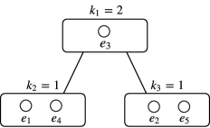
Figure 3: Bad example indicating the lack of negative dependency for optimal online policy of general laminar matroid.

We now propose a marking algorithm, parametrized by $\delta>0$, such that it guarantees the required concentration. Without loss of generality, assume $k_{B}\leq k_{B^{\prime}}$ for any two bins $B$ and $B^{\prime}$, whenever $B$ is a child of $B^{\prime}$ in the laminar tree. Let $L$ be the depth of the given instance (which we assume is constant in this section). Now, for every bin $B$ at depth $d$ of the laminar tree, i.e. when it has distance $d$ from the root, mark it as small if and only if $k_{B}\leq\frac{1}{\delta^{L-d}}$, and large otherwise (Fig. 4).

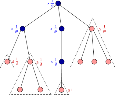
Figure 4: Depth-based marking for concentration.

The key idea here is that our proposed marking algorithm provides enough separation between a large bin and its small descendants. In fact, we partition the bins so that the capacity of every large bin is at least $\frac{1}{\delta}$ times the capacity of any of its small immediate descendant bins. This separation provides us with the required concentration bound.

Theorem 3.5.

Using the proposed marking algorithm and by setting $\delta=\frac{\epsilon^{2}}{\log(1/\epsilon)}$, Algorithm 2 is a $(1-O(\epsilon))$-approximation for the expected welfare of the optimal online policy in the laminar matroid Bayesian selection problem with depth $L$, and runs in time $\texttt{poly}(n)$ assuming $L$ and $\epsilon$ to be constant

Proof.

For every $B^{\prime}\in\mathscr{S}$, let $C_{B^{\prime}}$ denote the total number of elements picked from this bin. As maximal small bins $\mathscr{S}$ induce a partitioning over the set of all elements, and since Algorithm 2 runs an independent online policy in each bin $B^{\prime}\in\mathscr{S}$, random variables $\{C_{B^{\prime}}\}_{B^{\prime}\in\mathscr{S}}$ are mutually independent.

Now consider a large bin $B\in\mathscr{L}$ and suppose $B^{\prime}_{1},...,B^{\prime}_{m}$ be the small descendant bins that partition $B$. Moreover, assume bin $B$ is at depth $d$ of the laminar tree. Hence $k_{B}>\frac{1}{\delta^{L-d}}$ and $k_{B^{\prime}_{j}}\leq\frac{1}{\delta^{L-d-1}}$ for $j=1,...,m$. As the policy inside each small bin $B^{\prime}_{j}$ is a point-wise feasible policy, $C_{B^{\prime}_{j}}\leq k_{B^{\prime}_{j}}\leq\frac{1}{\delta^{L-d-1}}$. Moreover, linear program (LP₄) imposes a soft-constraint equal to $\sum_{t\in B^{\prime}_{j}}\mathbb{E}_{v_{t}}\left[\mathcal{X}^{*}_{t}(v_{t})\right]$ on each small bin. This soft-constraint should be respected in expectation by the final pricing policy (due to the construction of our randomized rounding scheme), so $\mathbb{E}[C_{B^{\prime}_{j}}]\leq\sum_{t\in B^{\prime}_{j}}\mathbb{E}_{v_{t}}\left[\mathcal{X}^{*}_{t}(v_{t})\right]$ for all $B^{\prime}_{j}$. Because of the global ex-ante constraints, these soft constraints should respect the large bin capacity constraints of the laminar matroid when large capacities are scaled down by a factor $(1-\epsilon)$. Therefore

$$\sum_{j=1}^{m}\mathbb{E}[C_{B^{\prime}_{j}}]\leq\sum_{j=1}^{m}\sum_{t\in B^{\prime}_{j}}\mathbb{E}_{v_{t}}\left[\mathcal{X}^{*}_{t}(v_{t})\right]=\sum_{t\in B}\mathbb{E}_{v_{t}}\left[\mathcal{X}^{*}_{t}(v_{t})\right]\leq k_{B}(1-\epsilon)$$

Now, by applying simple Chernoff bound for independent random variables $\{C_{B^{\prime}_{j}}\}_{j=1}^{m}$, we have (define the notation $\tilde{C}_{B^{\prime}_{j}}\triangleq C_{B^{\prime}_{j}}\cdot\delta^{L-d-1}$, so that it normalizes the total count to $[0,1]$):

$$\mathbb{P}[\displaystyle\sum_{j=1}^{m}C_{B^{\prime}_{j}}>k_{B}] =\mathbb{P}[\displaystyle\sum_{j=1}^{m}(C_{B^{\prime}_{j}}-\mathbb{E}[C_{B^{\prime}_{j}}])>k_{B}-\displaystyle\sum_{j=1}^{m}\mathbb{E}[C_{B^{\prime}_{j}}]]\leq\mathbb{P}[\displaystyle\sum_{j=1}^{m}(C_{B^{\prime}_{j}}-\mathbb{E}[C_{B^{\prime}_{j}}])>\epsilon k_{B}]$$

$$=\mathbb{P}[\displaystyle\sum_{j=1}^{m}(\tilde{C}_{B^{\prime}_{j}}-\mathbb{E}[\tilde{C}_{B^{\prime}_{j}}])>\epsilon\cdot\delta^{L-d-1}k_{B}]\leq\exp\left(-\frac{\epsilon^{2}\cdot\delta^{2(L-d-1)}\cdot k_{B}^{2}}{3\sum_{j=1}^{m}\mathbb{E}[\tilde{C}_{B^{\prime}_{j}}]}\right)$$

$$\leq\exp\left(-\frac{\epsilon^{2}\cdot\delta^{2(L-d-1)}\cdot k_{B}}{3}\right)$$

Now, for a particular element $t$, consider a path from the maximal small bin containing this element to the root of the laminar tree. This path consists of all the large bins that we need to check whether their capacities are exceeded or not at the time of the arrival of element $t$. Therefore, we need to take a union bound over all such bins. As mentioned earlier, without the loss of generality, we can assume the capacities of these large bins is an increasing sequence when indexed from lower-levels of the tree to the root (otherwise, bad events corresponding to nested bins of the same capacity merge while we take the union). Let $d^{*}$ be the depth of the maximal small bin containing $t$ in the laminar tree, and $B_{d}$ be the large bin along the mentioned path at depth $d$. By applying union bound:

$$\mathbb{P}[\exists B\in\mathscr{L}:t\in B,\displaystyle\sum_{t^{\prime}\in B}X_{t^{\prime}}>k_{B}]\leq\displaystyle\sum_{d=1}^{d^{*}+1}e^{\left(-\frac{\epsilon^{2}\delta^{2(L-d-1)}k_{B_{d}}}{3}\right)}\leq 2e^{\left(-\frac{\epsilon^{2}\delta^{2(L-d^{*}-1)}k_{B_{d^{*}}}}{3}\right)}\leq 2e^{\left(-\frac{\epsilon^{2}}{3\delta}\right)}=O(\epsilon)$$

where the last equality holds as $\delta=\frac{\epsilon^{2}}{\log(1/\epsilon)}$. Accordingly, with probability at least $1-O(\epsilon)$ none of these capacities are exceeded at the time that algorithm processes element $t$. Therefore, because of the linearity of expectation, Algorithm 2 achieves $(1-O(\epsilon))$ fraction of the expected social-welfare of the optimal online policy. Moreover, the linear program (LP₄) has size at most $O(n^{\frac{1}{\delta^{L}}})$, and hence the running time is $\texttt{poly}\left(n^{\left(\frac{\log(1/\epsilon)}{\epsilon^{2}}\right)^{L}}\right)$ by setting $\delta=\frac{\epsilon^{2}}{\log(1/\epsilon)}$. This running time is $\texttt{poly}(n)$ assuming $L$ and $\epsilon$ are constant. ∎

3.6 Discussion: extension to laminar over non-constant depth sub-problems.

As we saw earlier in Section 3.5, we can prove the correctness of our polynomial time approximation scheme only if the depth of the laminar family is constant. At the same time, as an observation, if one thinks of the production constrained Bayesian selection problem as an instance of the laminar Bayesian selection, then the depth of the corresponding laminar family will simply be $T+1$, and hence is not a constant. Yet, as we saw in Section 2, our approach in that section could yield to a PTAS. Can we still see this PTAS as a special case of our PTAS for the constant-depth laminar?

This discrepancy can easily be explained by extending our result for the constant depth laminar Bayesian selection to a generalization where every element is replaced by a sub-problem. With this view, in the production constrained Bayesian selection we indeed have only a 1-level tree (connecting the root to the type-specific sub-problems), and each leaf of this 1-level tree plays the role of one of the type-specific sub-problems. To make the analysis work, we require two things from each sub-problem. First, a local optimum online policy for each sub-problem, for possibly atomic or even non-positive value distributions, should be computable in polynomial time. Second, the selection rule of this local optimum online policy should satisfy the required negative cylinder dependency. Having these two properties, the proof of this section goes through, as by replacing each element with a group of negatively dependent elements we still have the required concentration. The proof of this generalization is basically the same, and so we omit to avoid redundancy.

4 Conclusion

We studied variations of the Bayesian selection problem. In this model, the goal is to serve a subset of arriving customers, maximizing the expected social welfare while respecting certain capacity or structural constraints. We presented two polynomial time approximation schemes when the set of allowable customers is restricted either by joint production/shipping constraints or a laminar family with constant depth. Our algorithms are based on rounding the solution of a hierarchy of linear programming relaxations that approximate the optimum solution within any degrees of accuracy. We take the first stab at designing polynomial time approximation schemes for Bayesian online selection problems; we hope that benchmarks similar to the type of linear programming hierarchy that we proposed here can lead to more insights, and new and interesting algorithms for this class of stochastic online optimization problems (or even beyond).

Appendix A Deferred Proofs of Section 2

Proof of Proposition 2.1.

We show how to round the linear programming solution of (LP₁). Let $\{\mathcal{X}^{*}_{t}(\vec{s},v),\mathcal{Y}^{*}_{t}(\vec{s})\}$ be the optimal solution of LP. First consider the following simple online randomized rounding scheme. It starts from all-zero assignment at time $t<1$. Now, suppose at time $t\geq 1$, the current state, i.e. vector of remaining capacities, is $\vec{s}$ and the realized value is $v_{t}=v$. The rounding algorithm first checks whether $\mathcal{Y}^{*}_{t}(\vec{s})$ is zero. If yes, it skips the buyer. Otherwise, it flips a coin with heads probability $\tfrac{\mathcal{X}^{*}_{t}(\vec{s},v)}{\mathcal{Y}^{*}_{t}(\vec{s})}$ and serves the buyer if the coin flips heads. Note that if we assume for all possible states $\vec{s^{\prime}}$, and all possible value $v^{\prime}$ the following holds so far:

$$\forall t^{\prime}<t:\mathbb{P}[\textrm{policy serves the buyer $t^{\prime}$ and the state at $t^{\prime}$ is $\vec{s}^{\prime}$}\nonscript\>|\nonscript\>\mathopen{}v_{t^{\prime}}=v^{\prime}]=\mathcal{X}^{*}_{t^{\prime}}(\vec{s}^{\prime},v^{\prime}),$$

$$\forall t\leq t:\mathbb{P}[\textrm{policy reaches the state $\vec{s^{\prime}}$ at $t^{\prime}$}]=\mathcal{Y}^{*}_{t^{\prime}}(\vec{s^{\prime}}),$$

then by progressing from $t$ to $t+1$, the same invariant holds because:

$$\mathbb{P}[\textrm{policy serves the buyer $t$ and the state at $t$ is $\vec{s}$}\nonscript\>|\nonscript\>\mathopen{}v_{t}=v]$$

$$= \mathbb{P}[\textrm{policy reaches the state $\vec{s^{\prime}}$ at $t^{\prime}$}]\cdot\tfrac{\mathcal{X}^{*}_{t}(\vec{s},v)}{\mathcal{Y}^{*}_{t}(\vec{s})}=\mathcal{Y}^{*}_{t}(\vec{s})\cdot\tfrac{\mathcal{X}^{*}_{t}(\vec{s},v)}{\mathcal{Y}^{*}_{t}(\vec{s})}=\mathcal{X}^{*}_{t}(\vec{s},v)$$

where in the first line we use that $v_{t}\sim F_{t}$ is independently drawn from the past. Moreover,

$$\mathbb{P}[\textrm{policy reaches the state $\vec{s}$ at $t+1$}]$$

$$=\mathbb{P}[\textrm{policy reaches the state $\vec{s}$ at $t$}]-\mathbb{P}[\textrm{policy serves the buyer $t$ and the state at $t$ is $\vec{s}$}]+$$

$$~{}~{}~{}~{}~{}\mathbb{P}[\textrm{policy serves the buyer $t$ and the state at $t$ is $\vec{s}+\vec{u}_{l_{t}}$}]$$

$$=\mathcal{Y}^{*}_{t}(\vec{s})-\mathbb{E}_{v_{t}}\left[\mathcal{X}^{*}_{t}(\vec{s},v_{t})\right]+\mathbb{E}_{v_{t}}\left[\mathcal{X}^{*}_{t}(\vec{s}+\vec{u}_{l_{t}},v_{t})\right]=\mathcal{Y}^{*}_{t+1}(\vec{s})$$

where $l_{t}$ is the day during which the $t^{\textrm{th}}$ buyer arrives, and in the last line we used the fact that the optimal solution of the LP satisfies the state evolution update rule (i.e. the LP constraint).

Putting all the pieces together, we conclude that the mentioned simple randomized rounding exactly simulates the probabilities predicted by the optimal LP solution, and hence is a point-wise feasible online policy with the same expected social welfare as the optimal value of the LP.

It only remains to show how an adaptive pricing mechanism with randomized tie breaking can also round the LP exactly. Let $\mathcal{Z}^{*}_{t}(\vec{s},v)\triangleq\tfrac{\mathcal{X}^{*}_{t}(\vec{s},v)}{\mathcal{Y}^{*}_{t}(\vec{s})}$ for every $v$ and $\vec{s}$ where $\mathcal{Y}^{*}_{t}(\vec{s})\neq 0$. By applying a simple coupling argument, we claim there should exist a threshold $\tau$ such that $\mathcal{Z}^{*}_{t}(\vec{s},v)=1$ for $v>\tau$, and $\mathcal{Z}^{*}_{t}(\vec{s},v)=0$ for $v<\tau$. If not, one can slightly move the allocation probability mass of the randomized rounding given $v_{t}=v$, i.e. $\mathcal{Z}^{*}_{t}(\vec{s},v)$, towards higher values, while maintaining the same expected marginal allocation $\mathbb{E}_{v_{t}}\left[X^{*}_{t}(\vec{s},v_{t})\right]$. This ensures that the state evolution probabilities will remain the same as the original randomized rounding, and hence this improved rounding algorithm can be coupled after time $t$ with the original randomized rounding (hence, will respect all the capacity constraints).

This new rounding algorithm achieves strictly more expected total value, a contradiction to the optimality of the original randomized rounding. Now, if $\mathcal{Y}^{*}_{t}(\vec{s})=0$ let $\tau_{t}(\vec{s})=+\infty$ (so that the adaptive pricing do not serve the buyer in this situation). Otherwise, let $\tau_{t}(\vec{s})$ be the threshold at which $\mathcal{Z}^{*}_{t}(\vec{s},v)$ switched to zero, and let $p_{t}(\vec{s})=\mathcal{Z}^{*}_{t}(\vec{s},\tau_{t}(\vec{s}))$. With these choices, the adaptive pricing with randomized tie breaking simulates the conditional probabilities $\mathcal{Z}^{*}_{t}(\vec{s},v)$ and couples with the original randomized rounding of the optimal LP solution, so it will be an optimal online policy. ∎

How to compute prices and tie-breaking probabilities in Proposition 2.1?.

Given the optimal assignment of LP₁, prices and tie-breaking probabilities can easily be computed. At any time $t$ and feasible state $\vec{s}$, find the minimum price $\tau_{t}(\vec{s})$ for which the probability that the buyer’s value is above the price is at most $\frac{\mathbb{E}_{v_{t}}\left[\mathcal{X}^{*}_{t}(\vec{s},v_{t})\right]}{\mathcal{Y}^{*}_{t}(\vec{s})}$. After finding $\tau_{t}(\vec{s})$, set the tie-breaking probability to $p_{t}(\vec{s})=\frac{1}{\mathbb{P}[v_{t}=\tau_{t}(\vec{s})]}\left(\frac{\mathbb{E}_{v_{t}}\left[\mathcal{X}^{*}_{t}(\vec{s},v_{t})\right]}{\mathcal{Y}^{*}_{t}(\vec{s})}-\mathbb{P}[v_{t}>\tau_{t}(\vec{s})]\right)$. An straightforward calculation shows this pricing policy has exactly the same state probabilities and expected social-welfare (LP objective) as of the LP optimal assignment. ∎

Appendix B Deferred Proofs of Section 3

Proof of Proposition 3.1.

Consider the optimal online policy and its induced feasible online policy for the sub-problem $B$. Let $\{\mathcal{X}_{t}(\vec{s},v_{t})\}_{t\in B}$ be the allocation probabilities and $\{\mathcal{Y}_{t}(\vec{s})\}_{t\in B}$ be the state evolution probabilities of this policy. First of all, clearly the objective function of the LP is equal to the expected social welfare of the online policy. Second, $\mathcal{Y}_{t_{0}}([k_{B^{\prime}}]_{B^{\prime}\in\mathscr{F}^{B}})=1$, as the policy has not yet picked any elements in $B$ when the first element in $B$ arrives. Moreover, the policy respects all the capacity constraints point-wise. Hence, in the resulting assignment $\mathcal{Y}_{t}(\vec{s})=0$ for $\vec{s}\in\partial\mathcal{S}^{B}$ and the global ex-ante constraints are satisfied.

The only tricky constraint remains to check is the Bellman update constraint of $\mathcal{P}^{B}$. In order to see the satisfaction of the constraint, note that the policy will reach state $\vec{s}$ at time $t$ if and only if either the state at time $t^{\prime}$ (i.e. the last time an element arrived in $B$) is $\vec{s}$ and the element at time $t^{\prime}$ is not selected, or the state at time $t$ is $\vec{s}+\vec{d}_{t^{\prime}}$ and the element at time $t^{\prime}$ is selected, evolving the state from $\vec{s}+\vec{d}_{t^{\prime}}$ to $\vec{s}+\vec{d}_{t^{\prime}}-\vec{d}_{t^{\prime}}=\vec{s}$. Therefore, the state evolution probabilities satisfy the Bellman update constraint. ∎

References

- Abolhassani et al. [2017] Melika Abolhassani, Soheil Ehsani, Hossein Esfandiari, MohammadTaghi HajiAghayi, Robert Kleinberg, and Brendan Lucier. Beating 1-1/e for ordered prophets. In Proceedings of the 49th Annual ACM SIGACT Symposium on Theory of Computing, pages 61–71. ACM, 2017.
- Alaei [2014] Saeed Alaei. Bayesian combinatorial auctions: Expanding single buyer mechanisms to many buyers. SIAM Journal on Computing, 43(2):930–972, 2014.
- Alaei et al. [2012] Saeed Alaei, MohammadTaghi Hajiaghayi, and Vahid Liaghat. Online prophet-inequality matching with applications to ad allocation. In Proceedings of the 13th ACM Conference on Electronic Commerce, pages 18–35. ACM, 2012.
- Alaei et al. [2015] Saeed Alaei, Jason Hartline, Rad Niazadeh, Emmanouil Pountourakis, and Yang Yuan. Optimal auctions vs. anonymous pricing. In Foundations of Computer Science (FOCS), 2015 IEEE 56th Annual Symposium on, pages 1446–1463. IEEE, 2015.
- Azar et al. [2014] Pablo D Azar, Robert Kleinberg, and S Matthew Weinberg. Prophet inequalities with limited information. In Proceedings of the twenty-fifth annual ACM-SIAM symposium on Discrete algorithms, pages 1358–1377. Society for Industrial and Applied Mathematics, 2014.
- Azar et al. [2018] Yossi Azar, Ashish Chiplunkar, and Haim Kaplan. Prophet secretary: Surpassing the 1-1/e barrier. In Proceedings of the 2018 ACM Conference on Economics and Computation, pages 303–318. ACM, 2018.
- Babaioff et al. [2015] Moshe Babaioff, Nicole Immorlica, Brendan Lucier, and S Matthew Weinberg. A simple and approximately optimal mechanism for an additive buyer. ACM SIGecom Exchanges, 13(2):31–35, 2015.
- Bellman [1954] Richard Bellman. The theory of dynamic programming. Bulletin of the American Mathematical Society, 60(6):503–515, 1954.
- Bhalgat et al. [2011] Anand Bhalgat, Ashish Goel, and Sanjeev Khanna. Improved approximation results for stochastic knapsack problems. In Proceedings of the twenty-second annual ACM-SIAM symposium on Discrete Algorithms, pages 1647–1665. Society for Industrial and Applied Mathematics, 2011.
- Cai et al. [2012] Yang Cai, Constantinos Daskalakis, and S Matthew Weinberg. Optimal multi-dimensional mechanism design: Reducing revenue to welfare maximization. In Foundations of Computer Science (FOCS), 2012 IEEE 53rd Annual Symposium on, pages 130–139. IEEE, 2012.
- Cai et al. [2016] Yang Cai, Nikhil R Devanur, and S Matthew Weinberg. A duality based unified approach to bayesian mechanism design. In Proceedings of the forty-eighth annual ACM symposium on Theory of Computing, pages 926–939. ACM, 2016.
- Chawla and Miller [2016] Shuchi Chawla and J Benjamin Miller. Mechanism design for subadditive agents via an ex ante relaxation. In Proceedings of the 2016 ACM Conference on Economics and Computation, pages 579–596. ACM, 2016.
- Chawla et al. [2010] Shuchi Chawla, Jason D Hartline, David L Malec, and Balasubramanian Sivan. Multi-parameter mechanism design and sequential posted pricing. In Proceedings of the forty-second ACM symposium on Theory of computing, pages 311–320. ACM, 2010.
- Chekuri et al. [2009] Chandra Chekuri, Jan Vondrák, and Rico Zenklusen. Dependent randomized rounding for matroid polytopes and applications. arXiv preprint arXiv:0909.4348, 2009.
- Chen et al. [2009] Ning Chen, Nicole Immorlica, Anna R Karlin, Mohammad Mahdian, and Atri Rudra. Approximating matches made in heaven. In International Colloquium on Automata, Languages, and Programming, pages 266–278. Springer, 2009.
- Dean et al. [2004] Brian C Dean, Michel X Goemans, and J Vondrdk. Approximating the stochastic knapsack problem: The benefit of adaptivity. In Foundations of Computer Science, 2004. Proceedings. 45th Annual IEEE Symposium on, pages 208–217. IEEE, 2004.
- Dubhashi and Ranjan [1998] Devdatt Dubhashi and Desh Ranjan. Balls and bins: A study in negative dependence. Random Structures and Algorithms, 13(2):99–124, 1998.
- Düetting et al. [2017] Paul Düetting, Michal Feldman, Thomas Kesselheim, and Brendan Lucier. Prophet inequalities made easy: Stochastic optimization by pricing non-stochastic inputs. In Foundations of Computer Science (FOCS), 2017 IEEE 58th Annual Symposium on, pages 540–551. IEEE, 2017.
- Esfandiari et al. [2017] Hossein Esfandiari, MohammadTaghi Hajiaghayi, Vahid Liaghat, and Morteza Monemizadeh. Prophet secretary. SIAM Journal on Discrete Mathematics, 31(3):1685–1701, 2017.
- Feldman et al. [2013] Michal Feldman, Hu Fu, Nick Gravin, and Brendan Lucier. Simultaneous auctions are (almost) efficient. In Proceedings of the forty-fifth annual ACM symposium on Theory of computing, pages 201–210. ACM, 2013.
- Feldman et al. [2016] Moran Feldman, Ola Svensson, and Rico Zenklusen. Online contention resolution schemes. In Proceedings of the twenty-seventh annual ACM-SIAM symposium on Discrete algorithms, pages 1014–1033. Society for Industrial and Applied Mathematics, 2016.
- Fu et al. [2018] Hao Fu, Jian Li, and Pan Xu. A ptas for a class of stochastic dynamic programs. arXiv preprint arXiv:1805.07742, 2018.
- Göbel et al. [2014] Oliver Göbel, Martin Hoefer, Thomas Kesselheim, Thomas Schleiden, and Berthold Vöcking. Online independent set beyond the worst-case: Secretaries, prophets, and periods. In International Colloquium on Automata, Languages, and Programming, pages 508–519. Springer, 2014.
- Gupta et al. [2016] Anupam Gupta, Viswanath Nagarajan, and Sahil Singla. Algorithms and adaptivity gaps for stochastic probing. In Proceedings of the twenty-seventh annual ACM-SIAM symposium on Discrete algorithms, pages 1731–1747. Society for Industrial and Applied Mathematics, 2016.
- Hajiaghayi et al. [2007] Mohammad Taghi Hajiaghayi, Robert Kleinberg, and Tuomas Sandholm. Automated online mechanism design and prophet inequalities. In AAAI, volume 7, pages 58–65, 2007.
- Halman et al. [2014] Nir Halman, Diego Klabjan, Chung-Lun Li, James Orlin, and David Simchi-Levi. Fully polynomial time approximation schemes for stochastic dynamic programs. SIAM Journal on Discrete Mathematics, 28(4):1725–1796, 2014.
- Hartline [2012] Jason D Hartline. Approximation in mechanism design. American Economic Review, 102(3):330–36, 2012.
- Immorlica et al. [2004] Nicole Immorlica, David Karger, Maria Minkoff, and Vahab S Mirrokni. On the costs and benefits of procrastination: Approximation algorithms for stochastic combinatorial optimization problems. In Proceedings of the fifteenth annual ACM-SIAM symposium on Discrete algorithms, pages 691–700. Society for Industrial and Applied Mathematics, 2004.
- Kleinberg and Weinberg [2012] Robert Kleinberg and Seth Matthew Weinberg. Matroid prophet inequalities. In Proceedings of the forty-fourth annual ACM symposium on Theory of computing, pages 123–136. ACM, 2012.
- Krengel and Sucheston [1978] Ulrich Krengel and Louis Sucheston. On semiamarts, amarts, and processes with finite value. Advances in probability and related topics, 4:197–266, 1978.
- Lee and Singla [2018] Euiwoong Lee and Sahil Singla. Optimal online contention resolution schemes via ex-ante prophet inequalities. arXiv preprint arXiv:1806.09251, 2018.
- Li and Yuan [2013] Jian Li and Wen Yuan. Stochastic combinatorial optimization via poisson approximation. In Proceedings of the forty-fifth annual ACM symposium on Theory of computing, pages 971–980. ACM, 2013.
- Lucier [2017] Brendan Lucier. An economic view of prophet inequalities. ACM SIGecom Exchanges, 16(1):24–47, 2017.
- Ma [2014] Will Ma. Improvements and generalizations of stochastic knapsack and multi-armed bandit approximation algorithms. In Proceedings of the twenty-fifth annual ACM-SIAM symposium on Discrete algorithms, pages 1154–1163. SIAM, 2014.
- Manshadi et al. [2012] Vahideh H Manshadi, Shayan Oveis Gharan, and Amin Saberi. Online stochastic matching: Online actions based on offline statistics. Mathematics of Operations Research, 37(4):559–573, 2012.
- Myerson [1981] Roger B Myerson. Optimal auction design. Mathematics of operations research, 6(1):58–73, 1981.
- Papadimitriou and Tsitsiklis [1987] Christos H Papadimitriou and John N Tsitsiklis. The complexity of markov decision processes. Mathematics of operations research, 12(3):441–450, 1987.
- Pemantle [2000] Robin Pemantle. Towards a theory of negative dependence. Journal of Mathematical Physics, 41(3):1371–1390, 2000.
- Rubinstein [2016] Aviad Rubinstein. Beyond matroids: Secretary problem and prophet inequality with general constraints. In Proceedings of the forty-eighth annual ACM symposium on Theory of Computing, pages 324–332. ACM, 2016.
- Samuel-Cahn et al. [1984] Ester Samuel-Cahn et al. Comparison of threshold stop rules and maximum for independent nonnegative random variables. the Annals of Probability, 12(4):1213–1216, 1984.
- Yan [2011] Qiqi Yan. Mechanism design via correlation gap. In Proceedings of the twenty-second annual ACM-SIAM symposium on Discrete Algorithms, pages 710–719. Society for Industrial and Applied Mathematics, 2011.