Decay of acoustic turbulence in two dimensions and implications
for cosmological gravitational waves

Abstract

Gravitational waves from a phase transition associated with the generation of the masses of elementary particles are within the reach of future space-based detectors such as LISA. A key determinant of the resulting power spectrum, not previously studied, is the lifetime of the acoustic turbulence which follows. We study decaying acoustic turbulence using numerical simulations of a relativistic fluid in two dimensions. Working in the limit of non-relativistic bulk velocities, with an ultra-relativistic equation of state, we find that the energy spectrum evolves towards a self-similar broken power law, with a high-wavenumber behaviour of $k^{-2.08\pm 0.08}$, cut off at very high $k$ by the inverse width of the shock waves. Our model for the decay of acoustic turbulence can be extended to three dimensions using the universality of the high-$k$ power law and the evolution laws for the kinetic energy and the integral length scale. It is used to build an estimate for the gravitational wave power spectrum resulting from a collection of shock waves, as might be found in the aftermath of a strong first order phase transition in the early universe. The power spectrum has a peak wavenumber set by the initial length scale of the acoustic waves, and a new secondary scale at a lower wavenumber set by the integral scale after a Hubble time. Between these scales a distinctive new power law appears. Our results allow more accurate predictions of the gravitational wave power spectrum for a wide range of early universe phase transition scenarios.

I Introduction

The first direct observation of gravitational waves in 2015 [1] started a new revolutionary era in gravitational wave astronomy. For the first time, it was possible to make observations without the limitations brought by detecting electromagnetic radiation or particles. Gravitational waves travel at the speed of light, and unlike electromagnetic radiation, interact extremely weakly with matter, travelling mostly undisturbed through the universe, carrying with them unfiltered information of their origins. These properties make them an outstanding probe of the pre-recombination era universe [2]. Sources of gravitational waves in the very early universe produce a stochastic gravitational wave background [3, 4] that could be detectable with future gravitational wave detectors [5, 6], like the upcoming Laser Interferometer Space Antenna (LISA) [7].

One potential source of contributions to the stochastic gravitational background of the very early universe is a first order cosmological phase transition [8, 9, 10, 11]. Such transitions proceed via the nucleation, expansion, and merger of bubbles containing the new low temperature phase [12, 13, 14, 15, 16]. The phase transition comes to an end when all bubbles have merged with the neighbouring bubbles so that the old phase has been replaced by the new one everywhere in the fluid, leaving behind a characteristic spectrum of sound waves [17, 18, 19, 20] and if the transition is strong enough, significant vorticity [21]. The sound waves are an important source of gravitational waves. They persist in the fluid long after the phase transition has completed, until dissipated away by the viscosity. Over time, these sound waves can steepen into shock waves. Such a statistically random field of shocks moving in various directions is known as acoustic turbulence [22, 23], and is the focus of this article.

Over the years the shock-containing compressional modes have received some study but to a much lesser degree when compared to vortical turbulence. Perhaps the most famous of such studies is that of the relatively simple Burgers’ equation [24, 25], which shares many of the properties seen in the Navier-Stokes equations, apart from the chaotic behaviour and randomness rising from small perturbations in the initial conditions. This is because it is possible to integrate Burgers’ equation explicitly. Burgers’ equation appears in the asymptotic limit in many physical situations, and has been extensively studied due to its simplicity.

As for the Navier-Stokes equations, there have been some earlier studies that deal with the compressional modes in fluids with a non-relativistic equation of state. Numerical simulations of the two- and three-dimensional Navier-Stokes equations with a longitudinal velocity component were performed by Porter, Pouquet and Woodward in Ref. [26] in the supersonic limit. They pay attention to the power laws seen in the energy spectra and the kinetic energy fractions between the longitudinal and transverse modes. The interactions between the compressible and rotational modes in a three-dimensional case were studied in 1990’s in Refs. [27, 28] with resolutions up to $1024^{3}$. Of the more cosmologically oriented papers using relativistic fluid equations, one worth highlighting is a paper by Pen and Turok [29] that contains one-, two- and three-dimensional simulations of shock formation in primordial acoustic oscillations.

In this paper we study two-dimensional decaying acoustic turbulence using numerical simulations with relativistic fluid equations and random initial conditions. The emphasis is on the profile of the generated shock waves, their effect on the shape of the energy spectrum, and the decay properties of the kinetic energy and the integral length scale. Using the obtained results, we also make an estimate for the gravitational wave power spectrum resulting from shocks in a three-dimensional fluid flow.

We have chosen to conduct the simulations in two dimensions for several reasons. The most important of these is that based on the existing literature, the shocks – amongst other phenomena – have the same properties, like the inertial range power laws in the energy spectrum, in two and three dimensions. However, the two-dimensional case is simpler to analyse: for example, it is easier to locate the shocks in two dimensions; some quantities, like the vorticity, are simpler (it being a scalar in 2D); and there are additional conserved quantities compared to 3D. In addition, there is the clear advantage of 2D being more computationally efficient, allowing for the use of larger grid sizes, increasing the dynamic range of the simulations. This makes it easier to study non-linear phenomena like turbulence and shocks. In 3D, the largest simulations to date have lattice sizes of $4200^{3}$ [19], and have not yet simulated sufficiently fast fluid flows for long enough to show the development of turbulence after a cosmological phase transition. Here, we simulate on grid sizes up to $10000^{2}$, for long enough to easily see the development and decay of shocks.

We also save some compute time by starting simulations with the velocity and density perturbations as a random field with given power spectra, rather than simulating the whole phase transition. This allows us to conclude that the effects we observe are not special to phase transitions. This is similar to the approach of Ref. [30], studying gravitational wave production by vortical turbulence, which starts its simulations with the Kolmogorov spectrum.

The contents of this article are as follows: Section II contains information about the fluid equations, details of the numerical simulations and the initial conditions, and lists some useful quantities used in characterising the state of the fluid. Section III concerns the results of our numerical simulations and is divided into several subsections. In Section III.1, an analytical form for the shock shape is derived using the fluid equations. Section III.2 focuses on the energy spectrum and its evolution over time, and in III.3 the decay of kinetic energy and the integral length scale is studied. The last subsection, III.4, takes a closer look at the transverse kinetic energy that arises from the longitudinal only initial conditions under these fluid equations. In Section IV an estimate is built for the gravitational wave power spectrum resulting from a collection of sound waves seen in our simulations. Two appendices are also included, Appendix A being about testing the results obtained in Section III.1 by conducting runs in a shock tube. Appendix B provides a more in depth look at the initial conditions and some more technical aspects of the simulations. Also listed are the runs used to obtain the tables and figures presented in this paper, and the initial conditions for each of the runs. In this paper we take the speed of light $c=1$.

II Methods

In this paper we study the evolution and properties of two-dimensional decaying acoustic turbulence using numerical simulations of a relativistic fluid. The equations we have employed are obtained from the relativistic fluid equations by expanding them to second order in first order small quantities that we have taken to be the non-relativistic bulk velocity v, and the bulk and shear viscosities. We also relate the pressure $p$ and energy density $\rho$ via the ultra-relativistic equation of state $p=c_{s}^{2}\rho$, where $c_{s}$ is the speed of sound parameter, which has the value $1/\sqrt{3}$ in the case of a radiation fluid. The derivation of the inviscid part of these equations is discussed in more detail in [31]. They can be written as

$$\frac{\partial\rho}{\partial t}+(1+c_{s}^{2})\nabla\cdot(\rho\textbf{v}) =0$$ (1)

$$\frac{\partial\textbf{v}}{\partial t}+\textbf{v}\cdot\nabla\textbf{v}-c_{s}^{2}\textbf{v}(\nabla\cdot\textbf{v})+\frac{c_{s}^{2}}{\rho(1+c_{s}^{2})}\nabla\rho =\frac{1}{1+c_{s}^{2}}\left[\eta\nabla^{2}\textbf{v}+\left(\frac{1}{3}\eta+\nu\right)\nabla(\nabla\cdot\textbf{v})\right]\,,$$ (2)

where $\eta$ and $\nu$ are the kinematic shear and bulk viscosity respectively. They enter the equations via the additions of the anisotropic stress tensor and the viscous bulk pressure to the energy momentum tensor. In the very early universe the Reynolds number is expected to be large and the shear viscosity to be dominant; its magnitude can be expressed in terms of the temperature and the electromagnetic gauge coupling parameter [32]. With our choice of scheme, viscosity is required to keep the numerical solution stable in cases where there is significant power in the longitudinal modes. In the longitudinal case shear and bulk viscosities also act in effectively the same way. The lack of an external forcing term means that the kinetic energy in the system decays over time, as it is being dissipated into internal energy by the viscosity at small length scales.

We define the spectral density $P(k)$ through the two-point correlation function of a homogenous and isotropic velocity field as

$$\left\langle v_{i}(\mathbf{k})v_{i}(\mathbf{k}^{\prime})\right\rangle=(2\pi)^{2}P(k)\delta(\mathbf{k}-\mathbf{k}^{\prime})$$ (3)

with $v_{i}(\mathbf{k})$ being the Fourier components of the velocity, related through the Fourier transform pair

$$v_{i}(\mathbf{k}) =\int v_{i}(\mathbf{r})e^{-i\mathbf{r}\cdot\mathbf{k}}\,d^{2}r$$ (4)

$$v_{i}(\mathbf{r}) =\frac{1}{(2\pi)^{2}}\int v_{i}(\mathbf{k})e^{i\mathbf{r}\cdot\mathbf{k}}\,d^{2}k\,,$$ (5)

where $\mathbf{k}$ is the wave vector. We define a quantity $E(k)$ through

$$E(k)=\frac{k}{4\pi}P(k)\,,$$ (6)

where $P(k)$ is the spectral density, such that

$$\frac{1}{2}\left\langle\textbf{v}^{2}\right\rangle=\int\limits_{0}^{\infty}E(k)\,dk\,,$$ (7)

from which we directly obtain the root mean square (rms) value of the velocity vector field. In a system with a non-relativistic equation of state, $E(k)$ is also the linear spectrum of the kinetic energy per unit mass, so we will refer to it as the energy spectrum. The true specific kinetic energy in our system is $(1+c_{\text{s}}^{2})\left\langle\textbf{v}^{2}\right\rangle$.

The velocity field is decomposed into longitudinal and transverse components so that

$$\textbf{v}=\textbf{v}_{\parallel}+\textbf{v}_{\perp}\,,$$ (8)

where the components fulfil the properties

$$\nabla\cdot\textbf{v}_{\perp}=0\,,\qquad\nabla\times\textbf{v}_{\parallel}=0\,.$$ (9)

This decomposition also splits the energy spectrum into two parts, $E(k)=E_{\parallel}(k)+E_{\perp}(k)$, where the longitudinal spectrum contains the contribution from acoustic turbulence, and the transverse part the vortical contributions associated with traditional fluid turbulence that consists of vortices of various sizes.

The fluid equations are integrated numerically using finite difference methods. Time integration is performed using the fourth order Runge-Kutta scheme, and spatial derivatives are evaluated with a second order central difference scheme. The spatial grid is a square with $N^{2}$ points and unit spacing. The time step size is chosen as $\Delta t=0.2\Delta x$, providing a stable numerical solution. Periodic boundary conditions are enforced on all edges of the grid. The corresponding reciprocal lattice is spanned by the wave vectors $\mathbf{k}_{i}$, whose elements obtain values in the range $[-\pi,\pi)$ with a spacing of $\Delta k=2\pi/(N\Delta x)$.

The initial conditions are given for the longitudinal and transverse components using an initial spectral density of the form

$$P(k)=A\frac{(k/k_{p})^{\beta_{0}}}{\left[1+(k/k_{p})^{\alpha_{0}/\gamma}\right]^{\gamma}}e^{-(k/k_{d})^{2}}\,.$$ (10)

The parameters $\alpha_{0}$ and $\beta_{0}$ set the initial values for the inertial range and low-$k$ power laws, $\gamma$ affects the shape around the peak of the spectrum, and $k_{p}$ is the initial wavenumber around which the peak is located. The inverse of $k_{p}$ deterimines the integral length scale $L$ characterizing the length scale at which most of the energy is located. We have also introduced an exponential suppression factor in order to reduce discretization effects at high wavenumbers. This suppression is controlled by the parameter $k_{d}$. Since we are interested in acoustic turbulence only, we set $P_{\perp}(k)=0$ initially, i.e. the initial velocity field is purely compressible. The Fourier components obtained from $P_{\parallel}(k)$ are given random phases in such a way that the resulting initial velocity field is real and statistically random. The energy density is initialized by writing it out as

$$\rho(\mathbf{r},t)=\rho_{0}+\delta\rho(\mathbf{r},t)\,$$ (11)

where the density perturbation $\delta\rho$ is initialized in the same way as the velocity components. More information about the execution of the simulations and their initial conditions can be found in Appendix B.

Next, we define some quantities that are useful in analysing the flows. We write the rms velocity of the longitudinal component as $\bar{v}=\sqrt{\left\langle\textbf{v}_{\parallel}^{2}\right\rangle}$, and define the integral length scale of the longitudinal component as

$$L=\frac{2}{\bar{v}^{2}}\int\limits_{0}^{\infty}\frac{1}{k}E_{\parallel}(k)\,dk\,.$$ (12)

From the initial values of these two quantities we can define a time scale,

$$t_{s}=L_{0}/\bar{v}_{0}$$ (13)

where $\bar{v}_{0}$ is the initial value of the rms longitudinal velocity, and $L_{0}$ is the initial value of the integral scale. In addition to the integral scale, there are other relevant length scales constructed from the effective viscosity $\mu=4\eta/3+\nu$, the rms velocity $\bar{v}$, and the quantity

$$\mathcal{D}=\left\langle(\nabla\cdot\textbf{v})^{2}\right\rangle,$$ (14)

the compressional part of the enstrophy, which can be used to quantify “shockiness” in the system. First, we have

$$\delta_{s}=\mu/\bar{v}\,,$$ (15)

which we shall see characterises the shock width. We also have the longitudinal counterparts of the Kolmogorov and Taylor microscales $L_{K}$ and $L_{T}$. We define the Kolmogorov microscale as

$$L_{K}=\left(\frac{\mu^{3}}{\epsilon}\right)^{1/6}\,,$$ (16)

where $\epsilon=-\dot{\mathcal{D}}$ is the dissipation rate of $\mathcal{D}$. From the equations of motion it follows that

$$\epsilon=\frac{4\mu}{1+c_{s}^{2}}\int\limits_{0}^{\infty}k^{4}E_{\parallel}(k)\,dk\,.$$ (17)

As in the case of vortical fluid turbulence, the Kolmogorov microscale specifies the length scale at which viscosity is dominant and dissipates kinetic energy into internal energy. The Taylor microscale is an intermediate length scale located between the integral and Kolmogorov length scales at which viscous effects become significant, and is defined by

$$L_{\text{T}}=\sqrt{\frac{\bar{v}^{2}}{\mathcal{D}}}\,.$$ (18)

The Taylor and Kolmogorov wavenumbers are defined as inverses of the corresponding length scales. We also define the longitudinal counterpart of the Reynolds number

$$\text{Re}=\frac{\bar{v}L}{\mu}\,,$$ (19)

that, as in the vortical only case, characterises the strength of non-linear effects in the flow, which in the longitudinal case means shocks. In other words, large values of the longitudinal Reynolds number lead to a formation of very strong and sharp shocks.

III Results

We have performed numerical simulations of acoustic turbulence with grid sizes of $N=4080$ and $N=10080$ with various initial power spectra (10) for the longitudinal component, leading to various shock formation times, and initial longitudinal Reynolds numbers in the range 16-223. We call runs with an initial Reynolds number that lies at the end of this range high Reynolds number runs. These kind of runs are obtained by increasing the initial rms velocity and also by increasing the initial integral length scale, which moves the top of the energy spectrum to lower wavenumbers. We have run for about 60 shock formation times in all of our runs to give the system enough time to show sufficient decay characteristics. A table listing each run and their initial conditions is found in Appendix B. In this section we shall present our findings from these runs focusing on the shape of the shocks, their impact on the energy spectrum, the decay of the longitudinal kinetic energy and the integral length scale, and the generation of transverse kinetic energy under these equations from the longitudinal only initial conditions.

III.1 Shock shape

In order to study the shape of the shock waves, we solve equations (1) and (2) for a single shock moving towards the positive x-axis using the ansatz

$$\rho(\mathbf{r},t)=L(k_{s}(x-ut)),\quad\vec{v}(\mathbf{r},t)=V(k_{s}(x-ut))\vec{e}_{x}\,.$$ (20)

Here $u$ denotes the shock velocity. The resulting differential equation is then written in terms of $\chi=k_{s}(x-ut)$ for $V(\chi)$ and is simplified by assuming that $V(\chi)\ll u$. Its solution is

$$V(x,t)=\frac{\sqrt{a^{2}+2bC}}{b}\tanh\left[k_{s}(x-x_{0}-ut)\right]-\frac{a}{b}\,,$$ (21)

where the parameters $a$ and $b$ can be written as:

$$a=u\left(1-\frac{c_{s}^{2}}{u^{2}}\right)$$ (22)

$$b=(1+c_{s}^{2})\left(\frac{c_{s}^{2}-1}{c_{s}^{2}+1}-\frac{c_{s}^{2}}{u^{2}}\right)\,.$$ (23)

The integration constant $C$ is fixed using the conditions that on the right side of the shock $V$ approaches the value $V_{+}$, and on the left side the value $V_{-}$ while the derivative of $V$ approaches zero on both sides. For a right-moving shock we also have $V_{-}>V_{+}$. These conditions fix $C$ as

$$C=aV_{+}+\frac{b}{2}V_{+}^{2}=aV_{-}+\frac{b}{2}V_{-}^{2}\,.$$ (24)

The shock velocity is solved from this equation and can be written in the form

$$u=c_{s}\left(1-\frac{2}{1+c_{s}^{2}}\xi\right)^{-\frac{1}{2}}\,,\quad\xi=\left(1+\frac{2}{\widetilde{\delta\rho}_{+}+\widetilde{\delta\rho}_{-}}\right)^{-1}$$ (25)

where $\widetilde{\delta\rho}_{+}$ and $\widetilde{\delta\rho}_{-}$ are the values of the fractional density perturbation on the left and right sides of the shock, obtained by replacing $V_{+}$ and $V_{-}$ using the relation between $V$ and the fractional density perturbation

$$V(x,t)=\frac{u}{1+c_{\text{s}}^{2}}\widetilde{\delta\rho}(x,t)\,,\quad\widetilde{\delta\rho}(x,t)=\frac{\delta\rho(x,t)}{\rho_{0}}.$$ (26)

Equation (25) gives us the expected result of the shock velocity always being larger than the speed of sound for a right-moving shock with $\widetilde{\delta\rho}_{+}=0$, since the smallest value $\xi$ can obtain is zero in the limit of the shock wave amplitude going to zero. It is also evident that the shock velocity increases with increasing amplitude.

The width of the shock is controlled by the parameter $k_{s}$ that can be written in terms of the above quantities as

$$k_{s}=\frac{3(1+c_{s}^{2})\sqrt{a^{2}+2bC}}{8\mu}$$ (27)

and whose inverse is of the same order of magnitude as the shock width $\delta_{s}$. The parameters $a$, $b$ and $C$ all increase with increasing shock velocity, which indicates that steep shocks are obtained when the amplitude of the shocks is large. Here the effects of the viscosities are clearly seen, with small viscosity values leading to steep shocks. We have conducted shock tube runs to study and verify the results obtained here by investigating shocks in a very narrow and long grid. These are discussed in Appendix A.

In our 2D simulations the initially smooth density and velocity fields generate multiple shock waves moving in various directions, after a time of order $t_{s}$. This can be seen in Figure 1, which on the left shows a contour plot of the density perturbation shortly after the shocks have formed. In the second plot on the right, the divergence of the velocity field has been plotted to highlight the shocks. Figure 2 shows zoomed in slices of the fractional density perturbation both in the high and low Reynolds number cases. In the case of the former, oscillations can be seen near the top of the shock, similar to the Gibbs phenomenon [33]. This limits the obtainable Reynolds numbers, as reducing the viscosity too much causes these oscillations to grow, eventually ruining the solution. This also has an effect on the shape of the energy spectrum around the Kolmogorov microscale, creating a bump in the spectrum at this wavenumber range.

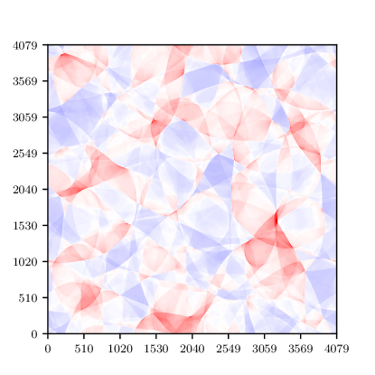
(a)

(b)

Figure 1: The density perturbation $\delta\rho$ of a $4080^{2}$ resolution run that has the same initial conditions as run 9 (a), and the divergence of the corresponding velocity field $\nabla\cdot\textbf{v}$ (b), showing the locations of the shocks at $t\approx 6.5t_{s}$.

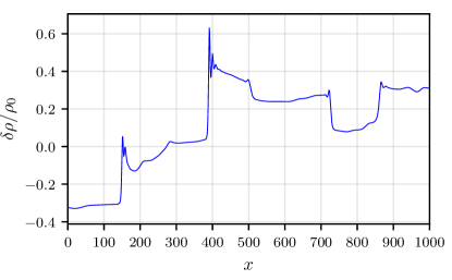
(a)

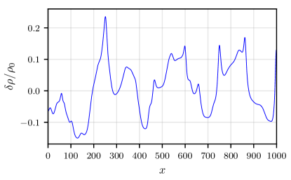
(b)

Figure 2: Zooms of the fractional density perturbation slices of the same $4080^{2}$ resolution run as in Figure 1 (a), and a similar moderate Reynolds number run (b) that has identical initial conditions to those of run 2. Both figures show the shocks after about $6.5$ shock formation times.

III.2 Shocks and the energy spectrum

Based on our simulations that use various different initial spectral densities (10), we find that as the initial conditions steepen into shocks, the features induced by the initial conditions near the peak of the energy spectrum are erased, and that the energy spectrum obtains a universal broken power law form whose power law values differ from those of the initial conditions. After a single shock formation time, the inertial range power law located between the integral length scale and the Taylor microscale settles into the well-known value of -2, first proposed and obtained by Burgers [34] for the one-dimensional Burgers equation, and later generalised to multiple dimensions in the case of the Euler and the continuity equation by Kadomtsev and Petviashvili [35].

The evolution of the inertial range power law in one of our runs has been plotted in Figure 3 as a function of the number of shock formation times. Due to strong oscillations in the spectrum at early times, the data for the plot has been obtained by fitting a power law $k^{-\varphi}$ to two intervals; between the Taylor and half the Kolmogorov wavenumber at early times when $t/t_{s}<0.6$, and between the integral wavenumber and the Taylor wavenumber otherwise. Early on, obtaining decent fits of the inertial range is obstructed by these oscillations, so we have tracked the evolution of the power law range of the initial conditions instead, which initially develops towards a similar power law value but at a higher wavenumber range. At $t/t_{s}=0.6$ the oscillations have weakened and the two ranges coincide, to a reasonable accuracy, so we have opted to change the limits of the fit at this particular time.

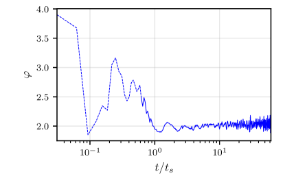
Figure 3: Evolution of the inertial range power law index obtained by fitting a power law $k^{-\varphi}$ to the data of run 9. The bounds of the fit are the Taylor and half times the Kolmogorov wavenumbers when $t/t_{s}<0.6$ (dashed curve) and the integral wavenumber and the Taylor wavenumber otherwise.

In order to study and determine the universal shape of the spectrum, we extract the time dependence from the spectrum. Figure 5 shows the time evolution of the spectrum with dark lines corresponding to late times. Over time the integral length scale $L$, introduced in section II, increases as evidenced by the shift of the peak of the spectrum towards small wavenumbers. Thus we fix the location of the peak by scaling the wavenumber by $L$, so that the spectrum becomes a function of $\kappa=L(t)k$. The other time dependent feature of the spectrum is the decay of the compressional kinetic energy $\mathcal{E}_{\parallel}$, which causes the magnitude of the spectrum to decrease. Thus, we write the spectrum in the form

$$E_{\parallel}(\kappa,t)=L(t)\mathcal{E}_{\parallel}(t)\Psi(\kappa)\,,\quad\kappa=L(t)k\,.$$ (28)

The function $\Psi(\kappa)$ is plotted in Figure 5 at even time intervals after the shocks have formed, and we see the spectra collapsing onto a single function on all but the very smallest length scales.

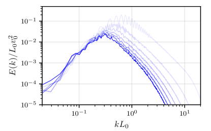
Figure 4: The scaled energy spectrum of run 2 plotted every $10t_{s}$ from $3t_{s}$ onwards. Dark colours correspond to late times.

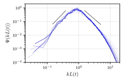
Figure 5: The energy spectra of Figure 5 collapsing into the function $\Psi(Lk)$. The black line above the inertial range describes the $k^{-2}$ power law, while the black line above the low-$k$ range goes like $k^{2.4}$.

In the range where the spectra collapse well, we model the function $\Psi$ by a broken power law form. We assume that this form holds at wavenumbers corresponding to length scales larger than the Taylor microscale, so that

$$\Psi(\kappa)=\Psi_{0}\frac{(\kappa/\kappa_{p})^{\beta}}{1+(\kappa/\kappa_{p})^{\alpha}}\,,\quad\kappa\ll L/L_{T}\,,$$ (29)

where $\beta$ is the low-$k$ power law index, and the inertial range power law is given by $\beta-\alpha$. From equation (28) it follows that the integral of $\Psi$ over all values of $\kappa$ must equal unity, and another condition follows from substituting (28) into the definition of the integral length scale in Equation (12). For both of these conditions to be satisfied simultaneously, the parameters $\Psi_{0}$ and $\kappa_{p}$ must fulfil

$$\Psi_{0}=\frac{\alpha}{\pi}\sin\left(\frac{\pi\beta}{\alpha}\right)$$ (30)

and

$$\kappa_{p}=\frac{\sin\left(\frac{\pi(\beta+1)}{\alpha}\right)}{\sin\left(\frac{\pi\beta}{\alpha}\right)}\,,$$ (31)

when $\beta-\alpha<-1$, meaning that these parameters get fixed by the normalisation condition and the choice of $L$ as the integral scale. In the high-$\kappa$ region where the collapse is not as good, and the function still changes a little over time. We ascribe this temporal behaviour to the changing shape of the shocks caused by the viscous dissipation. Thus, we expect the function $\Psi$ to be a broken power law modulated by a function that depends on the width of the shocks. To quantify the dilatation of the shocks, we use the dimensionless quantity $\mathcal{D}L^{2}/\mathcal{E}_{\parallel}$ to measure shockiness in the system, where $\mathcal{D}$ is defined through Eq. (14). The quantity $\nabla\cdot\mathbf{v}$, often called the dilatation, obtains large values at the locations of the shock waves briefly after shock formation in comparison to the values seen in the initial conditions, which leads to an increase in its rms value $\sqrt{\mathcal{D}}$. The dimensionless quantity is plotted in Figure 6, and a sharp increase in its value can be seen around one shock formation time, after which the quantity decreases, as the shocks deteriorate.

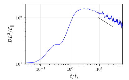
Figure 6: Plot of the dimensionless quantity $\mathcal{D}L^{2}/\mathcal{E}_{\parallel}$ that is used to measure shockiness of the system as a function of shock formation times. The data for the plot has been obtained from run 9. The black line indicates a $t^{-0.4}$ power law.

In order to determine what impact the shocks have on the energy spectrum, we follow the method presented in Ref. [36] to find the form of the two-dimensional energy spectrum using the one-dimensional spectrum. The one-dimensional energy spectrum of a tanh shock is obtained using the Fourier transform and has the form

$$E_{1}(k)=|\mathcal{F}(\tanh(k_{s}x))|^{2}=\frac{\pi^{2}}{k_{s}^{2}}\text{csch}^{2}\left(\frac{\pi k}{2k_{s}}\right)\,,$$ (32)

which can be related to the $D$-dimensional spectrum by separating the wavevector $\mathbf{k}$ into two parts; $\mathbf{k}_{1}$ and its transverse projection $\mathbf{k}_{\perp}$ and then by integrating over the latter

$$E_{1}(k_{1}) =\int E_{D}(|\mathbf{k}|)d\mathbf{k}_{\perp}$$ (33)

$$=\frac{1}{2}\Omega_{D-1}\int\limits_{k_{1}^{2}}^{\infty}E_{D}(s)(s^{2}-k_{1}^{2})^{\frac{D-3}{2}}\,ds^{2}\,.$$ (34)

where $\mathbf{k}=\mathbf{k}_{\perp}+\mathbf{k}_{1}$ and $\Omega_{D-1}$ is the solid angle of the ($D-2$)-sphere. For $D=2$ the equation can be written as

$$E_{1}(k_{1})=\int\limits_{k_{1}^{2}}^{\infty}\frac{E_{2}(\sqrt{u})}{\sqrt{u-k_{1}^{2}}}\,du\,.$$ (35)

Now we can use the property, that $E_{1}$ is a first order Liouville-Weyl fractional integral [37] of $E_{2}$ to solve for the two-dimensional spectrum, yielding

$$E_{2}(k)=\frac{1}{\pi}\int\limits_{k^{2}}^{\infty}\frac{1}{\sqrt{u-k^{2}}}\frac{d}{du}E_{1}(\sqrt{u})\,du\,.$$ (36)

Substituting Equation (32), changing the variable, and defining

$$E_{2}=\frac{\pi^{2}}{k_{s}^{3}}\mathcal{I}\,,\quad P=\frac{\pi k}{2k_{s}}$$ (37)

allows us to write (36) as

$$\mathcal{I}(P)=\int\limits_{1}^{\infty}\frac{ds}{\sqrt{s^{2}-1}}\frac{\cosh(Ps)}{\sinh^{3}(Ps)}\,.$$ (38)

The integral in $\mathcal{I}$ does not have a closed form solution, but its asymptotic behaviour at small and large values of the argument can be found to be

$$\mathcal{I}(P)\sim\begin{cases}\dfrac{\pi}{4P^{3}}\,,\quad P\ll 1\\ \\ 2\sqrt{\dfrac{\pi}{P}}e^{-2P}\,,\quad P\gg 1\end{cases}\,.$$ (39)

We now propose the function $\Psi(\kappa)$ to have the form

$$\Psi(\kappa)=\widetilde{\Psi}_{0}\frac{(\kappa/\kappa_{p})^{\beta+3}}{1+(\kappa/\kappa_{p})^{\alpha}}\mathcal{I}\left(\frac{\pi\kappa}{2\kappa_{s}}\right)\,,$$ (40)

where $\kappa_{s}=k_{s}L$. Note that the parameter $\beta$ still denotes the low-$k$ power law. Figure 7 shows $\Psi(\kappa)$ obtained from simulation data in comparison to the fit resulting from using the equation above. It is seen that the fit is very good in the high-$\kappa$ region. At the wavenumber range between the Taylor and the Kolmogorov wavenumbers, the fit deviates a bit from the simulation data, leading to slightly steeper values for the inertial range power than $k^{-2}$. The fit in this range can be improved by increasing the complexity of the fitting function, for example, by using a double broken power law instead, but for our purposes we deem Equation (40) to be a good enough estimate for the spectral collapse function $\Psi$.

Figure 7: The function $\Psi(\kappa)$, where the blue line is the curve obtained from simulation data of run 2 at $t\approx 20t_{s}$, and the dashed red line is a fit using Equation (40). The obtained values for the fit parameters are $\widetilde{\Psi}_{0}=0.0034$, $\alpha\approx 4.801$, $\beta\approx 2.013$. $\kappa_{p}\approx 0.976$, and $\kappa_{s}=12.541$.

III.3 Decay of longitudinal kinetic energy

Energy is dissipated into heat by the viscosity at small length scales, and since our fluid equations do not contain a forcing term, the total kinetic energy decreases over time. Figure 8 plots the kinetic energy normalised by its initial value for several runs as a function of the number of shock formation times. It is seen that after about 10 shock formation times the kinetic energy decays following a power law form.

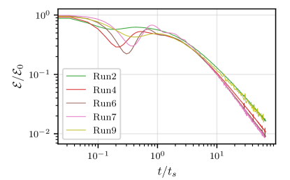
Figure 8: The kinetic energy normalised by the initial value plotted for some the runs listed in Table 4 as a function of the shock formation time.

In order to find an analytical function that models the kinetic energy behaviour seen in the figure, we have applied the analysis made by Saffman in Ref. [38], but to the longitudinal-only case instead. The starting point is the relation describing the kinetic energy decay due to viscous dissipation, which for the fluid equations (1) and (2) can be shown to be

$$\frac{1}{2}\frac{d\left\langle\textbf{v}^{2}_{\parallel}\right\rangle}{dt}=-\frac{2\mu}{1+c_{\text{s}}^{2}}\int\limits_{0}^{\infty}k^{2}E_{\parallel}(k)\,dk\,,$$ (41)

when the vorticity $\nabla\times\mathbf{v}$ is zero. There is some vorticity generated from longitudinal only initial conditions under these fluid equations, as discussed in the next section, but the transverse kinetic energy is still small enough in comparison to the longitudinal kinetic energy for the above equation to be approximately valid. After the shocks have formed, the energy spectrum has the familiar behaviour of $k^{-2}$ in the inertial range. According to Saffman, in the case of Burger’s equation, the spectrum in the inertial range has the form

$$E_{\parallel}(k)=\frac{\mathcal{L}\overline{J}^{2}}{4\pi k^{2}}\,,$$ (42)

which we assume to also hold for the fluid equations employed in this paper by applying the physical interpretations of $\mathcal{L}$ and $\overline{J}^{2}$ to the longitudinal case. Here $\mathcal{L}$ is the mean length of shocks per unit area, and $\overline{J}^{2}$ is the mean square jump in velocity across the shock. In analogy to [38], we cut off the integral at the wavenumber corresponding to the length scale of the shock width $\delta_{s}$ and substitute (42) into (41), which after integration gives

$$\frac{1}{2}\frac{d\left\langle\textbf{v}^{2}_{\parallel}\right\rangle}{dt}=-\frac{\mu}{2\pi(1+c_{s}^{2})}\frac{\mathcal{L}\overline{J}^{2}}{\delta_{s}}\propto\frac{\bar{v}^{3}(t)}{L(t)}\,,$$ (43)

where to obtain the latter expression we have used the proportionality relations

$$\quad\mathcal{L}\propto L^{-1}\,,\quad\overline{J}^{2}\propto\bar{v}^{2}\,,$$ (44)

and the definition for the shock width $\delta_{s}$ in equation (15). Now in order to make progress, we need to find a relation between the time behaviour of the integral length scale and the rms velocity. To this end, we write the spectrum in the form

$$E_{\parallel}(k,t)=D(t)\frac{\left[k/k_{p}(t)\right]^{\beta}}{1+\left[k/k_{p}(t)\right]^{\alpha}}\,,$$ (45)

where the prefactor $D(t)$ contains the time dependence of the spectral magnitude. Here we have ignored the high-$k$ behaviour of the spectrum found in the previous section. Now in the low-$k$ power law range, when $k\ll k_{p}$, the spectrum becomes

$$E_{\parallel}(k,t)\approx D(t)k_{p}(t)^{-\beta}k^{\beta}\,.$$ (46)

The very low-$k$ end of the spectrum stays mostly unchanged, maintaining its magnitude and power law index, as seen in Figure 5. Hence, it can be approximated that

$$D(t)k_{p}(t)^{-\beta}=\text{const.}$$ (47)

Substituting this spectrum into Equation (7) gives

$$\frac{1}{2}\left\langle\textbf{v}_{\parallel}^{2}\right\rangle=D(t)\int\limits_{0}^{\infty}\frac{\left[k/k_{p}(t)\right]^{\beta}}{1+\left[k/k_{p}(t)\right]^{\alpha}}\,dk\,.$$ (48)

Using this form for the spectrum leads to an overestimation of the integral, since we have ignored the high-$k$ behaviour, but we argue that this does not affect the value of the energy significantly, since the largest contribution to the integral comes from the energy containing scales around the peak of the spectrum, and the contributions from scales smaller than the Taylor microscale are small in comparison. After a change of variables $s=k/k_{p}$ the integral becomes

$$\frac{1}{2}\left\langle\textbf{v}_{\parallel}^{2}\right\rangle=D(t)k_{p}(t)\int\limits_{0}^{\infty}\frac{s^{\beta}}{1+s^{\alpha}}\,ds\,.$$ (49)

Since the power laws stay the same after the shocks have formed, the parameters $\alpha$ and $\beta$ are mostly constant. Thus, the integral gives approximately a constant value, and by using the definition of the rms velocity and relation (47) with $k_{p}(t)^{-1}=L(t)$, we get

$$\bar{v}^{2}(t)L(t)^{\beta+1}=\text{const.}\equiv\xi^{-(\beta+1)}\,.$$ (50)

Using this, we can now solve Equation (43) for the energy $\mathcal{E}=\left\langle\textbf{v}_{\parallel}^{2}\right\rangle/2=\bar{v}^{2}/2$ with the initial condition ${\mathcal{E}(t=0)=\mathcal{E}_{0}}$, yielding

$$\mathcal{E}(t)=\frac{\mathcal{E}_{0}}{\left(1+C\frac{t}{t_{s}}\right)^{\zeta}}\,,\quad\zeta=\frac{2(\beta+1)}{\beta+3}\,,$$ (51)

where in the denominator we have used (50) to write the constant $\xi$ in terms of the initial value of the integral length scale $L_{0}$ and the initial energy $\mathcal{E}_{0}$, resulting in $\xi(2\mathcal{E}_{0})^{(\beta+3)/(2(\beta+1))}=L_{0}^{-1}\bar{v}_{0}=t_{s}^{-1}$, which is used as an estimate for the shock formation time. We have also absorbed all constants into the parameter $C$, whose value depends on the values of the prefactors of the relations listed in Equation (44). Without knowing the numerical values of the prefactors, the value of $C$ can be obtained by fitting. Based on our fits detailed later in this section, its typical value lies in the range between 0.29 and 0.47. With the help of the above result, Equation (50) can be used to find $L(t)$, which reads as

$$L(t)=L_{0}\left(1+C\frac{t}{t_{s}}\right)^{\lambda}\,,\quad\lambda=\frac{2}{\beta+3}\,.$$ (52)

The integral length scales of some of the runs featured in table 4 of Appendix B are plotted in Figure 9 against time in units of $t_{s}$ the shock formation time.

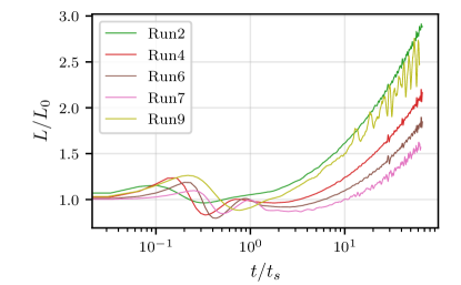
Figure 9: The longitudinal integral length scale normalised by the initial value plotted for multiple runs as a function of the number of shock formation times.

The results obtained for the power law values as functions of the low-$k$ power law $\beta$ in equations (51) and (52) coincide with those found by similar methods for three-dimensional classical vortical turbulence [39].

Equations (51) and (52) can now be used as fitting functions to the curves seen in Figures 8 and 9, and the obtained power law indices can then be compared to the analytical ones by measuring the low-$k$ power law index $\beta$ of each run. The fits to the kinetic energy and the integral length scale are constrained to the shock containing phase by using fitting ranges whose lower boundary lies in the range $t/t_{s}\geq 1$. In these ranges the inertial range has a power law of $k^{-2}$ and the fitting equations are valid. Figure 10 shows a pair of such fits for a single run. We have varied the lower bound of the fit to all data points in the range $1\leq t/t_{s}\leq 3$ and averaged over the results to obtain the averaged power law indices $\hat{\zeta}$ and $\hat{\lambda}$.

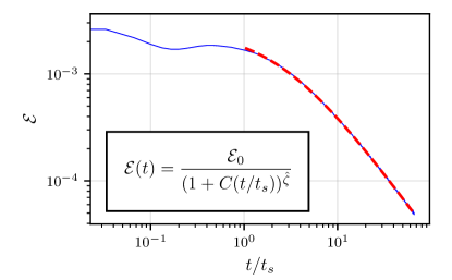
(a)

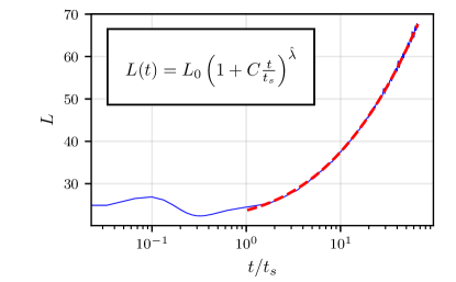
(b)

Figure 10: Fits of the functions (51) and (52) (red dashed curves) to the time evolution of the kinetic energy (a) and the integral length scale (b) of run 2 (blue curves). The fitting range is $t/t_{s}\geq 1$ and the parameter values obtained are $\mathcal{E}_{0}\approx 0.00263$, $\zeta\approx 1.207$, and $C\approx 0.391$ for the kinetic energy, and $L_{0}\approx 20.8$, $\lambda\approx 0.346$ and $C\approx 0.455$ for the integral length scale.

The low-$k$ power law indices are measured by fitting a broken power law, akin to that in Equation (45), on a suitable wavenumber range and averaging the obtained values for the fit parameters over times $8\leq t/t_{s}\leq 12$, which in our simulations results to around 120 data points on average. The suitable range in question has been chosen to be $k\in[1/6L,1/L_{T}]$, which contains the inertial range and a sufficient amount of the low-$k$ power law. Time averaging like this is necessary because there are oscillations in the spectrum that the fitting algorithm is sensitive to. We have used the standard deviations of the time averaging to quantify the strength of these oscillations.

It is also possible to derive relations between $\beta$, $\zeta$, and $\lambda$ that can be used to test the robustness of the theory by comparing to the values obtained from the simulations by fitting. Such relations have been obtained in Refs. [40, 41] by considering appropriate scaling of the energy spectrum and by making use of the rescaling invariance of the hydrodynamic equations. Here, one relation follows immediately from Equation (50), which requires

$$\lambda(\beta+1)-\zeta=0$$ (53)

for it to be valid. This relation can also be obtained directly from the power laws in equations (51) and (52). A relation containing only $\zeta$ and $\lambda$ can also be derived by replacing $\beta$ in the equation above by using either of these two equations, giving

$$\zeta-2(1-\lambda)=0\,.$$ (54)

Table 1 lists the averaged power law indices and the standard deviations obtained from fits to the time evolutions of the kinetic energy and the integral length scale. Power laws obtained from time averaging are denoted by hats, and alongside them are the power laws obtained from equations (51) and (52) using the values obtained for the time averaged low-$k$ power law $\hat{\beta}$. These values are listed in Table 2 alongside $\hat{\alpha}$ and the averaged value of the inertial range power law $\widehat{\beta-\alpha}$. Also listed are the standard deviations of these averages, denoted by sigmas, the initial low-$k$ power law index of the energy spectrum $\beta_{0}$ and the initial high-$k$ power law $\beta_{0}-\alpha_{0}$. The errors obtained from the fitting covariances are negligible in comparison to the standard deviations of the time fluctuations in all of these cases. We have also measured the magnitude of the statistical fluctuations resulting from different initial random phases given to the Fourier velocity components by making runs with the same initial conditions but with different random seeds. Based on these runs, the fluctuations are found to be either smaller or at the largest comparable in magnitude to the standard deviations in Tables 1 and 2. The values in these two tables are used to test the relations (53) and (54), which are listed in Table 3 along with their standard deviations obtained from the error propagation formula. These are denoted as $\Delta C_{i}$ where the index $i$ marks the column of the table (the run ID column being column 0). These relations are also plotted in a $\zeta\lambda$-coordinate system in Figure 11 where different low-$k$ power law values correspond to lines with different slopes converging at the origin [41]. The diagonal solid black line is the curve $\zeta=2(1-\lambda)$ of Equation (54). The error bars for the data points obtained from Table 1 are smaller than the data point markers and are thus not drawn in the figure. The scaling law following from the self-similarity is fulfilled well, with the value of zero lying within the margin of error, whereas the one using the scaling invariance is not as good due to the small standard deviations in the values of $\zeta$ and $\lambda$.

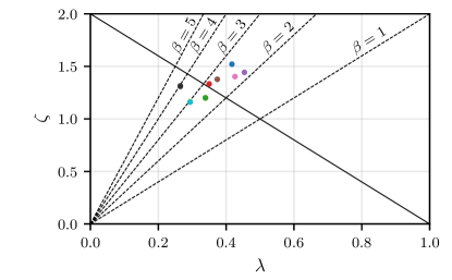
Figure 11: A $\zeta\lambda$-plot that illustrates the relations in equations (53) and (54). The diagonal solid black line is the curve $\zeta=2(1-\lambda)$. The data points for each run have been obtained using the values of $\hat{\zeta}$ and $\hat{\lambda}$ from Table 1.

ID	$\hat{\zeta}$	$\zeta$	$\hat{\lambda}$	$\lambda$	$\sigma_{\zeta}$	$\sigma_{\lambda}$
$\rule{0.0pt}{12.91663pt}{\color[rgb]{0.12109375,0.46484375,0.70703125}1}$	$1.521$	$1.294$	$0.417$	$0.353$	$1.09\text{\times}{10}^{-02}$	$7.48\text{\times}{10}^{-03}$
${\color[rgb]{1,0.49609375,0.0546875}2}$	$1.201$	$1.252$	$0.339$	$0.374$	$2.58\text{\times}{10}^{-03}$	$1.43\text{\times}{10}^{-03}$
${\color[rgb]{0.171875,0.62890625,0.171875}3}$	$1.200$	$1.252$	$0.339$	$0.374$	$2.56\text{\times}{10}^{-03}$	$1.42\text{\times}{10}^{-03}$
${\color[rgb]{0.83984375,0.15234375,0.15625}4}$	$1.333$	$1.284$	$0.350$	$0.358$	$1.08\text{\times}{10}^{-02}$	$5.07\text{\times}{10}^{-03}$
${\color[rgb]{0.58203125,0.40234375,0.7421875}5}$	$1.443$	$1.246$	$0.454$	$0.377$	$1.85\text{\times}{10}^{-02}$	$1.48\text{\times}{10}^{-02}$
${\color[rgb]{0.55078125,0.3359375,0.29296875}6}$	$1.377$	$1.359$	$0.374$	$0.320$	$1.53\text{\times}{10}^{-02}$	$7.96\text{\times}{10}^{-03}$
${\color[rgb]{0.890625,0.46484375,0.76171875}7}$	$1.403$	$1.352$	$0.426$	$0.324$	$1.83\text{\times}{10}^{-02}$	$1.32\text{\times}{10}^{-02}$
${\color[rgb]{0.49609375,0.49609375,0.49609375}8}$	$1.307$	$1.330$	$0.265$	$0.335$	$4.54\text{\times}{10}^{-03}$	$6.60\text{\times}{10}^{-03}$
${\color[rgb]{0.73828125,0.7421875,0.1328125}9}$	$1.164$	$1.296$	$0.294$	$0.352$	$3.07\text{\times}{10}^{-03}$	$2.07\text{\times}{10}^{-03}$
${\color[rgb]{0.08984375,0.74609375,0.8125}10}$	$1.160$	$1.237$	$0.294$	$0.381$	$3.38\text{\times}{10}^{-03}$	$1.88\text{\times}{10}^{-03}$
${\color[rgb]{0.1875,0.1875,0.1875}11}$	$1.314$	$1.422$	$0.265$	$0.289$	$7.46\text{\times}{10}^{-03}$	$4.15\text{\times}{10}^{-03}$

Table 1: Time averaged fit parameters for the kinetic energy and integral length scale power laws $\hat{\zeta}$ and $\hat{\lambda}$, obtained by fitting the curves seen in Figure 10 so that the lower boundary of the fitting range uses all data points in the range $1\leq t/t_{s}\leq 3$, and by averaging over the results. Also listed are the standard deviations, and the predicted values for the power laws given by equations (51) and (52) by using the values for the time averaged low-$k$ power law $\hat{\beta}$ listed in Table 2.

ID	$\beta_{0}$	$\beta_{0}-\alpha_{0}$	$\hat{\alpha}$	$\hat{\beta}$	$\widehat{\beta-\alpha}$	$\sigma_{\alpha}$	$\sigma_{\beta}$	$\sigma_{\beta-\alpha}$
$\rule{0.0pt}{12.91663pt}{\color[rgb]{0.12109375,0.46484375,0.70703125}1}$	$4$	$-8$	$3.576$	$2.669$	$-0.907$	$0.368$	$0.167$	$0.363$
${\color[rgb]{1,0.49609375,0.0546875}2}$	$3$	$-3$	$4.464$	$2.348$	$-2.116$	$0.072$	$0.113$	$0.069$
${\color[rgb]{0.171875,0.62890625,0.171875}3}$	$3$	$-3$	$4.464$	$2.349$	$-2.115$	$0.072$	$0.113$	$0.068$
${\color[rgb]{0.83984375,0.15234375,0.15625}4}$	$4$	$-5$	$4.182$	$2.586$	$-1.596$	$0.522$	$0.440$	$0.189$
${\color[rgb]{0.58203125,0.40234375,0.7421875}5}$	$5$	$-15$	$4.238$	$2.305$	$-1.933$	$0.426$	$0.299$	$0.182$
${\color[rgb]{0.55078125,0.3359375,0.29296875}6}$	$5$	$-5$	$4.986$	$3.240$	$-1.745$	$0.381$	$0.453$	$0.139$
${\color[rgb]{0.890625,0.46484375,0.76171875}7}$	$9$	$-6$	$5.258$	$3.176$	$-2.082$	$0.261$	$0.264$	$0.027$
${\color[rgb]{0.49609375,0.49609375,0.49609375}8}$	$5$	$-2$	$4.891$	$2.967$	$-1.924$	$0.443$	$0.464$	$0.050$
${\color[rgb]{0.73828125,0.7421875,0.1328125}9}$	$3$	$-3$	$4.693$	$2.683$	$-2.010$	$0.710$	$0.739$	$0.052$
${\color[rgb]{0.08984375,0.74609375,0.8125}10}$	$3$	$-3$	$4.374$	$2.243$	$-2.131$	$0.669$	$0.681$	$0.017$
${\color[rgb]{0.1875,0.1875,0.1875}11}$	$7$	$-4$	$5.970$	$3.916$	$-2.055$	$0.514$	$0.530$	$0.026$

Table 2: The initial low-$k$ power law of energy spectrum $\beta_{0}$ and the initial inertial range power law $\beta_{0}-\alpha_{0}$, and the same parameters after the shocks have formed obtained by time averaging the results obtained from broken power law fits of Equation (45) over the interval $8\leq t/t_{s}\leq 12$, denoted by hats. The last three columns list the standard deviations for the time fluctuations of the parameters $\alpha$ and $\beta$, and the inertial range power law.

ID	$\hat{\lambda}(\hat{\beta}+1)-\hat{\zeta}$	$\hat{\zeta}-2(1-\hat{\lambda})$	$\Delta C_{1}$	$\Delta C_{2}$
$\rule{0.0pt}{12.91663pt}{\color[rgb]{0.12109375,0.46484375,0.70703125}1}$	$0.008$	$0.354$	$0.076$	$1.85\text{\times}{10}^{-02}$
${\color[rgb]{1,0.49609375,0.0546875}2}$	$-0.066$	$-0.122$	$0.039$	$3.85\text{\times}{10}^{-03}$
${\color[rgb]{0.171875,0.62890625,0.171875}3}$	$-0.066$	$-0.122$	$0.039$	$3.82\text{\times}{10}^{-03}$
${\color[rgb]{0.83984375,0.15234375,0.15625}4}$	$-0.078$	$0.033$	$0.155$	$1.48\text{\times}{10}^{-02}$
${\color[rgb]{0.58203125,0.40234375,0.7421875}5}$	$0.056$	$0.351$	$0.145$	$3.49\text{\times}{10}^{-02}$
${\color[rgb]{0.55078125,0.3359375,0.29296875}6}$	$0.209$	$0.125$	$0.173$	$2.21\text{\times}{10}^{-02}$
${\color[rgb]{0.890625,0.46484375,0.76171875}7}$	$0.376$	$0.255$	$0.126$	$3.21\text{\times}{10}^{-02}$
${\color[rgb]{0.49609375,0.49609375,0.49609375}8}$	$-0.256$	$-0.163$	$0.126$	$1.40\text{\times}{10}^{-02}$
${\color[rgb]{0.73828125,0.7421875,0.1328125}9}$	$-0.080$	$-0.247$	$0.218$	$5.15\text{\times}{10}^{-03}$
${\color[rgb]{0.08984375,0.74609375,0.8125}10}$	$-0.206$	$-0.252$	$0.201$	$5.06\text{\times}{10}^{-03}$
${\color[rgb]{0.1875,0.1875,0.1875}11}$	$-0.013$	$-0.157$	$0.142$	$1.12\text{\times}{10}^{-02}$

Table 3: Numerical values for the relations of equations (53) and (54) that are obtained using the fit parameters in Tables 1 and 2. The last two columns contain the standard deviations of the relations in columns 1 and 2 obtained using the standard deviations of the fit parameters with the error propagation formula.

III.4 Generation of transverse kinetic energy

In our simulations we see an emergence of small amounts of transverse kinetic energy from longitudinal-only initial conditions. In order to study the vorticity generation more closely, we can take a look at the vorticity equation, obtained by taking a curl of Equation (2). The equation can be written for the vorticity $\omega=\nabla\times\textbf{v}$, which in two-dimensional case can be treated as a scalar, giving

$$\frac{\partial\omega}{\partial t}+(1-2c_{s}^{2})\omega(\nabla\cdot\textbf{v}) +(1-c_{s}^{2})(\textbf{v}\cdot\nabla)\omega$$ (55)

$$-c_{s}^{2}\textbf{v}\times\nabla^{2}\textbf{v}=\frac{\eta}{1+c_{s}^{2}}\nabla^{2}\omega\,.$$

From this it follows that if initially $\omega=0$

$$\frac{\partial\omega}{\partial t}=c_{s}^{2}\textbf{v}\times\nabla(\nabla\cdot\textbf{v})\,,$$ (56)

meaning that there is a vorticity generating term resulting from the last term on the left hand side of (2), giving rise to some transverse kinetic energy even when the initial conditions contain only longitudinal modes.

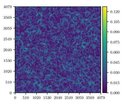
(a) $v(x,y)=|\mathbf{v}|$

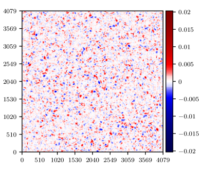
(b) $L\omega(x,y)$

(c) $v(x,y)=|\mathbf{v}|$

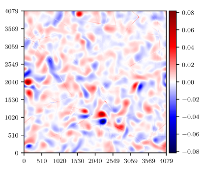
(d) $L\omega(x,y)$

Figure 12: The magnitude of the velocity field $|\textbf{v}|$ (a) and the corresponding vorticity field $\omega=\nabla\times\mathbf{v}$ scaled by the integral length scale (b) of a moderate Reynolds number $4080^{2}$ resolution run after about 13 shock formation times. Figures (c) and (d) show the same quantities for a high Reynolds number run at the end of the run at about $t=67t_{s}$. The runs have the same initial conditions as runs 2 and 9. In Figures (b) and (d) vortex-like structures can be seen, appearing in pairs of different signs.

In the simulations we see that early on the vorticity field attains its largest values in the regions containing overlapping or colliding shocks. This is illustrated in Figures 12a and 12b that show the magnitude of the velocity field and the corresponding vorticity that has been scaled by the integral length scale to obtain a dimensionless quantity. As the shocks overlap with each other, their amplitude increases, and regions with much higher amplitudes than seen in the initial conditions are formed, shown in the figure in yellow. The largest values of vorticity right after the shocks are formed are obtained around these regions, shown as thin short dark red lines in the contour plot. These features are short-lived and change location as the shocks travel. The other part of the vorticity field after shock formation is the background vorticity that changes slowly in comparison to the vorticity from shock collisions, and contains vortex-like structures that often appear in pairs of different signs. Over time as the shocks get dissipated, the background vorticity becomes dominant, with the shocks being only faintly visible in comparison, as seen in Figure 12d, which plots the dimensionless vorticity field at the very end of a run. The higher the Reynolds number of the run is, the higher the generated transverse kinetic energy is relative to the longitudinal kinetic energy. In Figure 13 the energy fraction $\mathcal{E}_{\perp}/\mathcal{E}_{\parallel}$ has been plotted for several runs, and the group of curves with the highest values corresponds to the high Reynolds number runs. It shows that the transverse kinetic energy is still small compared to the longitudinal kinetic energy, even after 60 shock formation times.

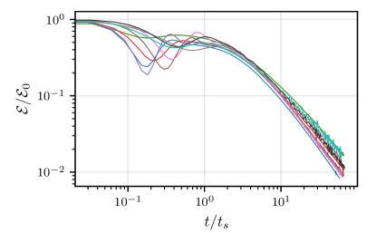
Figure 20: Figure 8 but all runs featured in table 4 are included. The runs have been colour coded to match the colours found in the ID columns of the tables here and in all other figures containing multiple runs to allow for distinguishability.

Runs 3 and 10 contain only bulk viscosity. We find that in the longitudinal case, both the bulk and the shear viscosity affect the fluid almost in an identical way. Runs 2 and 3, and 9 and 10 have the same initial conditions and random phases, with the only difference being the viscosity type. The values for the viscosities in these runs are chosen so that the value of the effective viscosity is the same. In the longitudinal case, these pairs of runs produce results that are very close to each other, which can also be seen from the plots of longitudinal quantities, such as in Figures 20, 21 of Appendix C, and 11, where the runs overlap, or from the tables of the previous section.

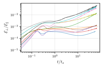
Figure 22: Figure 13 but all runs featured in table 4 are included. The high Reynolds number runs in the range 160-230, and the low Reynolds number runs in the range 10-60 are clearly separated into two groups by at least an order of magnitude, with the high Re runs having higher transverse kinetic energy. The exception is the low Re bulk viscosity only run (ID 3, green), which joins the high Re curves in the end. It has identical initial conditions to run 2 (orange) apart from the viscosity type.

The same is not true in the transverse case, as is evident by Figures 13 and 22, where the curves of the previously mentioned run pairs clearly separate from each other some time after the start of the run, with the bulk viscosity only run having a larger transverse kinetic energy at the end in both cases (see Table 4 in appendix B for the colour and viscosity type of each run in the case of Figure 22). This is because in the shear viscosity only case the dissipation of energy is larger, as under these fluid equations the dissipation due to viscosity can be shown to be

$$\frac{1}{2}\frac{d\left\langle\textbf{v}^{2}\right\rangle}{dt}=\begin{cases}-\frac{2\mu}{1+c_{\text{s}}^{2}}\int\limits_{0}^{\infty}k^{2}E(k)\,dk\,,\quad\text{when }\nabla\times\textbf{v}=0\\ -\frac{2\eta}{1+c_{\text{s}}^{2}}\int\limits_{0}^{\infty}k^{2}E(k)\,dk\,,\quad\text{when }\nabla\cdot\textbf{v}=0\end{cases}$$ (57)

meaning that for the transverse component the viscous dissipation is caused only by the shear viscosity. This also strongly affects the shape of the transverse energy spectrum at large-$k$ between the bulk and shear-viscosity only runs.

The focus of this paper is the study of the longitudinal case, and thus there is more potential work to be done in studying the transverse case under these fluid equations. The transverse only case (incompressible flow) has been extensively studied and forms part of the standard understanding of turbulence presented in textbooks (see e.g. Ref. [39]).

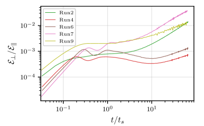
Figure 13: Development of the ratio of the transverse to longitudinal kinetic energy of several runs with time, in units of the shock formation time $t_{s}$. The high Reynolds number runs 7 and 9, and the low Reynolds number runs 2 and 4 are clearly separated into two groups by at least an order of magnitude, with the high Re runs having higher transverse kinetic energy. The exception is the low Re bulk viscosity only run (ID 2, green), which joins the high Re curves at the end of the run.

IV Estimate for the gravitational wave power spectrum

While there are no gravitational waves in two dimensions, we can estimate the gravitational wave power spectrum generated by shocks in three dimensions by using the results in Ref. [35], according to which the energy spectrum maintains the $k^{-2}$ inertial range power law in any number of space dimensions. By assuming the energy spectrum to have a simple broken power law form, the GW power spectrum can be obtained by adapting standard methods [42, 43, 44, 45, 46, 20].

The source of the gravitational waves is taken to be the shear stresses resulting from a velocity field consisting of randomly distributed sound waves, generated on a timescale long compared the light-crossing time of any important scales in the velocity field. The resulting GW power spectrum can be calculated from the unequal time velocity field correlators for the system. Our calculation assumes that the shock lifetime $t_{s}$ is much less than a Hubble time, meaning that the expansion of the universe can be approximated by setting the velocities to zero after a Hubble time [18]. It is also assumed that the fluid velocities are non-relativistic, and that the velocity can be treated as a Gaussian random field, with any non-Gaussianity leading to negligible contributions to the connected four-point correlator. As the initial velocity field steepens into shocks, the velocity field loses its Gaussianity but we assume the deviation from Gaussianity to be small, so that the correlator can still be approximately treated as Gaussian. Measuring the unequal time correlators for a collection of shock waves to test the validity of this assumption stands as possible future work.

We begin by citing Equation (3.46) of Ref. [20], which gives the growth rate of the gravitational wave power spectrum $\mathcal{P}_{\text{gw}}$ as

$$\frac{1}{H_{*}}\frac{d}{dt}\mathcal{P}_{\text{gw}}=3\left(\Gamma\bar{v}^{2}\right)^{2}(H_{*}L)\frac{(kL)^{3}}{2\pi^{2}}\tilde{P}_{\text{gw}}(kL)\,,$$ (58)

where $H_{*}$ is the Hubble rate at the time of the transition and $\Gamma$ is the mean adiabatic index of the fluid. We take $\Gamma=(1+c_{s}^{2})=4/3$, as appropriate for an ultrarelativistic fluid. The final factor in the expression is a dimensionless spectral density function, defined as

$$\tilde{P}_{\text{gw}}(y)=\frac{1}{4\pi yc_{s}} \left(\frac{1-c_{s}^{2}}{c_{s}^{2}}\right)^{2}\int\limits_{z_{-}}^{z_{+}}\frac{dz}{z}\frac{(z-z_{+})^{2}(z-z_{-})^{2}}{z_{+}+z_{-}-z}$$ (59)

$$\times\tilde{P}_{v}(z)\tilde{P}_{v}(z_{+}+z_{-}-z)\,,$$

where $z_{\pm}=y(1\pm c_{s})/(2c_{s})$, $z=qL$, and $\tilde{P}_{v}(z)$ is the scaled velocity spectral density, which is related to the actual spectral density as

$$P_{v}(qL)=L^{3}\bar{v}^{2}\tilde{P}_{v}(qL)$$ (60)

with $q$ being the wavenumber. The relation between the energy spectrum and the spectral density in 3D is

$$E(k)=\frac{k^{2}}{2\pi^{2}}P_{v}(k)\,.$$ (61)

On the other hand, the energy spectrum can also be written in terms of the collapse function $\Psi$ as seen in Equation (28), from which it follows that

$$P_{v}(z)=\pi^{2}L^{3}\bar{v}^{2}\frac{\Psi(z)}{z^{2}}\,.$$ (62)

Now for the function $\Psi(z)$ we use the broken power law form of Equation (29) that by using Equation (60) gives

$$\tilde{P}_{v}(z)=\frac{\Psi_{0}\pi^{2}}{z_{p}^{2}}\frac{(z/z_{p})^{\beta-2}}{1+(z/z_{p})^{\alpha}}\,.$$ (63)

Here the parameter $\kappa_{p}$ of Equation (29) has been denoted with $z_{p}$ to coincide notationally with $z$ and is fixed in terms of $\alpha$ and $\beta$ along with $\Psi_{0}$ through Equations (30) and (31). Using this and Equation (59), and integrating Equation (58) with respect to time with a change of variable ${z=kLs}$ gives the following expression for the gravitational wave power spectrum

$$\frac{1}{(H_{*}L_{0})^{2}} \mathcal{P}_{\text{gw}}(k,t_{H_{\star}})=\frac{3\pi\Psi_{0}^{2}\Gamma^{2}(1-c_{s}^{2})^{2}}{8L_{0}^{2}z_{p}^{4}c_{s}^{5}}k^{5}$$ (64)

$$\times\int\limits_{0}^{t_{H_{\star}}}dt\,\bar{v}^{4}(t)L^{6}(t)\int\limits_{s_{-}}^{s_{+}}ds\,I(s,t)$$

where $t_{H_{\star}}$ is the lifetime of the GW source, which we recall is taken to be the Hubble time at the time of the phase transition, [18]. The integrand $I$ has the form

$$I(s,t)=\frac{(s-s_{+})^{2}(s-s_{-})^{2}[s(s_{+}+s_{-}-s)/s_{p}^{2}(t)]^{\beta-3}}{s_{p}^{2}(t)[1+[s/s_{p}(t)]^{\alpha}][1+[(s_{+}+s_{-}-s)/s_{p}(t)]^{\alpha}]}\,,$$ (65)

with $s_{p}(t)=z_{p}/kL(t)$, and $s_{\pm}=(1\pm c_{s})/(2c_{s})$ Now we write the time integral only in terms of the integral scale $L(t)$ by relating it to $\bar{v}(t)$ using equation (50) and substituting the time development Equations (51) and (52) into it (while keeping in mind that $\mathcal{E}=\bar{v}^{2}/2$). Because of the relation between the power law indices in Equation (53) the time dependence vanishes and the equation can be written in the form

$$\bar{v}^{2}(t)=\bar{v}_{0}^{2}\left(\frac{L(t)}{L_{0}}\right)^{-(\beta+1)}\,.$$ (66)

Here $\bar{v}_{0}$ denotes the initial value of the rms velocity. Using this, the time integral in Equation (64) can be written as

$$\int\limits_{0}^{t_{H_{\star}}}dt\,\bar{v}^{4}(t)L^{6}(t)=\bar{v}_{0}^{4}L_{0}^{6}\int\limits_{0}^{t_{H_{\star}}}dt\,\left(\frac{L(t)}{L_{0}}\right)^{2(2-\beta)}\,.$$ (67)

Next we make a change of variables $\tau=kL(t)/z_{p}=s_{p}^{-1}$ in the time integral. This is tantamount to integrating over the integral length scale, which in the scenario considered here is a monotonically increasing quantity with time. The time differential can be related to the differential of this new variable by using Equation (52), which yields

$$dt=\frac{z_{p}}{\lambda Ck\bar{v}_{0}}\left(\frac{\tau}{\tau_{0}}\right)^{1/\lambda-1}\,d\tau\,,$$ (68)

where $\lambda$ is the decay power law of the integral length scale, $C$ is a decay parameter whose inverse gives the number of shock formation times that it takes for the flow to start decaying, and $\tau_{0}=kL_{0}/z_{p}$. Now, the $s$ integrand can also be written as

$$I(s,\tau)=\tau^{2(\beta-2)}I_{\tau}(s,\tau)\,,$$ (69)

where

$$I_{\tau}(s,\tau)=\frac{(s-s_{+})^{2}(s-s_{-})^{2}\left[s(s_{+}+s_{-}-s)\right]^{\beta-3}}{\left[1+(\tau s)^{\alpha}\right]\left[1+\tau^{\alpha}(s_{+}+s_{-}-s)^{\alpha}\right]}\,,$$ (70)

meaning that the factor of $\tau$ resulting from Equation (67) ends up cancelling with that coming from the $s$ integrand. The Equation (64) now becomes

$$\frac{1}{(H_{*}L_{0})^{2}}\mathcal{P}_{\text{gw}}(k)=\frac{3\pi\Psi_{0}^{2}z_{p}\Gamma^{2}(1-c_{s}^{2})^{2}}{8c_{s}^{5}}$$ (71)

$$\times\left(\frac{kL_{0}}{z_{p}}\right)^{4}\tau_{0}^{2\beta-1/\lambda-3}\int\limits_{\tau_{0}}^{\tau_{H_{\star}}}d\tau\,\tau^{1/\lambda-1}\int\limits_{s_{-}}^{s_{+}}ds\,I_{\tau}(s,\tau)\,,$$

where $\tau_{H_{\star}}=kL(t_{H_{\star}})/z_{p}$, and in the prefactor the powers of $k$ and $L_{0}$ are equal, so that they can be written in terms of $\tau_{0}=kL_{0}/z_{p}$. It is worth noting that with this formulation the integration limits also depend on the wavenumber $k$. We can now write the power law index $\lambda$ in terms of the low-$k$ power law index of the energy spectrum $\beta$ using the relation between them in Equation (52). We then factorise the result and write it in the form

$$\frac{1}{(H_{*}L_{0})^{2}}\mathcal{P}_{\text{gw}}(kL_{0},\tau_{H_{\star}})=\frac{\bar{v}_{0}^{3}}{C}\mathcal{N}S(kL_{0},\tau_{H_{\star}})\,,$$ (72)

where the numerical factor $\mathcal{N}$ is determined by the speed of sound in the fluid and the power law parameters $\alpha$ and $\beta$ appearing in the energy spectrum and has the form

$$\mathcal{N}=\frac{3\pi}{8}\frac{(\beta+3)\Psi_{0}^{2}z_{p}}{2}\frac{\Gamma^{2}(1-c_{s}^{2})^{2}}{c_{s}^{5}}\,.$$ (73)

The function $S(kL_{0},\tau_{H_{\star}})$ determines the shape of the spectrum, and can be written as

$$S(kL_{0},\tau_{H_{\star}})=\tau_{0}^{(3\beta-1)/2}\int\limits_{\tau_{0}}^{\tau_{H_{\star}}}d\tau\,\tau^{(\beta+1)/2}\int\limits_{s_{-}}^{s_{+}}ds\,I_{\tau}(s,\tau)\,.$$ (74)

Using Equation (74), we have plotted the shape of the GW power spectrum numerically. In the three-dimensional case the low-$k$ power law index of the energy spectrum $\beta$ is not expected to be the same as in 2D, and should be determined by numerical simulations. After the phase transition has completed, the fluid contains shocks and has the $k^{-2}$ power law at the inertial range. For this estimate, we have assumed a value of $\beta=4$, and taken $\alpha=6$ to obtain the correct value for the high-$k$ power law. The spectrum is then obtained by numerically integrating the two integrals that appear in (74) for a given ratio $L(t_{H_{\star}})/L_{0}$, which we have taken to be 6.1 for illustrative purposes when plotting the spectrum in Figure 14.

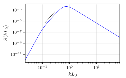
Figure 14: The function $S(kL_{0})$ obtained numerically from Equation (74) with parameter values $\alpha=6$, $\beta=4$, and $L(t_{H_{\star}})/L_{0}=6.1$. A bend in the spectrum at the low-$k$ end is seen at $kL_{0}\simeq z_{p}L_{0}/L(t_{H_{\star}})\simeq 0.1$. The black line demonstrates a power law of $k^{5.5}$.

The figure highlights an interesting aspect in the low-$k$ end of the spectrum, in that there is a change in the low-$k$ power law index around $kL_{0}\simeq z_{p}L_{0}/L(t_{H_{\star}})\simeq 0.095$, after which the power law changes from a steeper $k^{9}$ power law to a shallower power law of $k^{5.5}$. The location where this change occurs is determined by the lifetime of the source $t_{H_{\star}}$ through the ratio $L(t_{H_{\star}})/L_{0}$, so that the shallower power law appears in the range

$$z_{p}L_{0}/L(t_{H_{\star}})\lesssim kL_{0}\lesssim z_{p}\,.$$ (75)

Therefore, for short enough lifetimes, where the integral scale does not have enough time to grow significantly compared to its initial value, the range is short and close to the peak, meaning that effectively only the steeper slope is obtained, and for long lifetimes, where $L(t_{H_{\star}})>>L_{0}$, the bend occurs at very small wavenumbers close to the origin, so that the spectrum effectively only possesses the shallower slope. In the first case, the shock formation time $t_{s}$ is close in magnitude to the duration of the GW source $t_{H_{\star}}$, which is the Hubble time. Hence only short-lived source $t_{s}\ll t_{H_{\star}}$, as assumed here, will show the intermediate power law.

The power law behaviour of the GW power spectrum can be inspected by extracting the wavenumber behaviour of Equation (72) in different limits. At very small wavenumbers fulfilling the condition $\tau\ll 1$ for any $\tau\in[\tau_{0},\tau_{H_{\star}}]$ the integral over $s$ yields essentially a constant, from which it follows that

$$\frac{1}{(H_{*}L_{0})^{2}}\mathcal{P}_{\text{gw}}(k)\propto k^{2\beta+1}\,,$$ (76)

which for $\beta=4$ gives the value of the power law index seen in Figure 14. At large wavenumbers, so that $\tau\gg 1$ for any $\tau\in[\tau_{0},\tau_{H_{\star}}]$, it can be approximated

$$I_{\tau}(s,\tau)\approx\frac{(s-s_{+})^{2}(s-s_{-})^{2}\left[s(s_{+}+s_{-}-s)\right]^{\beta-\alpha-3}}{\tau^{2\alpha}}\,,$$ (77)

which means that the $s$-integral yields a constant once more, and after integrating over $\tau$, the $k$-dependence is found to be

$$\frac{1}{(H_{*}L_{0})^{2}}\mathcal{P}_{\text{gw}}(k)\propto k^{2(\beta-\alpha)+1}\,,$$ (78)

which for acoustic turbulence gives the power law of $k^{-3}$ at high wavenumbers. To touch on the intermediate power law seen in Figure 14, we need to understand the behaviour of the $\tau$-integrand in the regime where the $s$-integral does not yield a constant. To this end, we rewrite the integrals of Equation (74) in the form

$$\frac{1}{(H_{*}L_{0})^{2}}\mathcal{P}_{\text{gw}}(k)\propto k^{\frac{3\beta-1}{2}}\int\limits_{\tau_{0}}^{\tau_{H_{\star}}}f(\tau)\,,$$ (79)

where the function $f(\tau)$ denotes the integrand

$$f(\tau)=\tau^{\frac{\beta+1}{2}}\int\limits_{s_{-}}^{s_{+}}ds\,I_{\tau}(s,\tau)\,.$$ (80)

This function has been obtained numerically by using the same parameter values as in Figure 14, and is plotted in Figure 15.

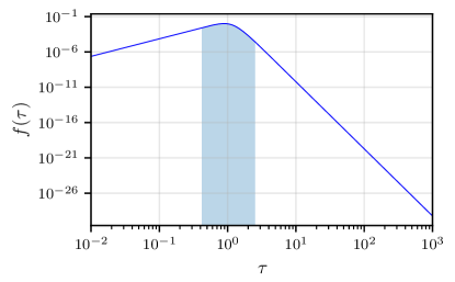
Figure 15: The integrand function $f(\tau)$ (see Eq. 80) plotted using the same parameter values as in Figure 14. The highlighted area shows the part of the curve contributing to the GW power spectrum at $kL_{0}=0.24$, which lies roughly in the middle of the intermediate power law range.

Since the integration limits depend on the wavenumber $k$, a different part of this curve is integrated for each value of $k$. It turns out that the intermediate power law is obtained at wavenumbers for which the integration range spans the peak of the function $f(\tau)$, that is, when the separation between $\tau_{H_{\star}}$ and $\tau_{0}$ is larger than the width of the peak in the integrand $f(\tau)$, which is located approximatively in the range $0.5\lesssim\tau\lesssim 2$. The width of the integration range for a given $k$ is determined by the the ratio $L(t_{H_{\star}})/L_{0}$. When it is large, the peak is panned even for small wavenumbers, resulting in the narrower power law at low-$k$, and when it is small, the integration range is narrow and does not span the peak entirely for any $k$ so that only the steeper power law is obtained. For the wavenumbers in the intermediate power law range, the integral over $f(\tau)$ is effectively a constant, since the largest contribution to the integral is obtained around the peak, which is spanned for all such wavenumbers, and since the contributions from the edges of the integration range are small in comparison. Therefore, it follows that in the intermediate power law range the GW power spectrum goes as

$$\frac{1}{(H_{*}L_{0})^{2}}\mathcal{P}_{\text{gw}}(k)\propto k^{\frac{3\beta-1}{2}}\,,$$ (81)

giving the power law seen in Figure 14 when $\beta=4$.

To conclude, apart from giving a power law of $k^{-3}$ in the high-$k$ range, the decay of the shocks also induces a change in the low-$k$ power law, going from $k^{2\beta+1}$ to a shallower $k^{(3\beta-1)/2}$ one, over a range depending on the integral scale of the fluid flow after a Hubble time. Note that the rate at which the flow was originally generated may also appear as a scale in the gravitational wave power spectrum, below which another power law may apply [46]. We have assumed that this happens at a lower wavenumber than any considered here.

V Conclusions

We have studied decaying acoustic turbulence using two-dimensional numerical simulations with the emphasis being on the impact of the shocks upon the energy spectrum, and on the decay of the kinetic energy. Conducting the simulations in two dimensions allows for better computational efficiency and the use of larger grid sizes in comparison to 3D, which leads to there being more dynamic range in the wavenumber space. Two-dimensional systems are also simpler to analyse and in the case of shocks share some properties with three-dimensional systems. By making use of the universality of the power spectra, the obtained two-dimensional decay properties and power laws of the system have been applied in three dimensions to calculate an estimate for the gravitational wave power spectrum resulting from a collection of shock waves.

The longitudinal energy spectrum of the fluid can be written in terms of the longitudinal kinetic energy, integral scale, and the dimensionless function $\Psi(kL)$ as seen in Equation (28). The function $\Psi(kL)$ has the property that it maintains its shape over time at length scales above the dissipation range. Using the tanh shock profile obtained from the fluid equations, we have presented an analytical universal form for this function, which is found to be a broken power law modulated by an integral function $\mathcal{I}$ that is shown in Equation (38). This function depends on the steepness of the shocks via the wavenumber parameter $k_{s}$ appearing in the argument of the tanh shocks. Between the wavenumbers corresponding to the integral scale and the Taylor microscale, the power law is found to be $k^{-2.08\pm 0.08}$, which agrees very well with the $k^{-2}$ power law associated with acoustic turbulence [35], obtained as an inverse-variance weighted average of the measurements in Table 2. At lower wavenumbers, using the same method, the power law is $k^{\beta}$, with $\beta=2.50\pm 0.31$.

In order to find the time evolution of the longitudinal kinetic energy, we have used the $k^{-2}$ inertial range power law, and the self-similarity of the spectrum at low-$k$ to find equations (51) and (52), the latter of which describes the decay of the longitudinal integral length scale. At times much larger than the shock formation time, these produce power law forms, where the values of the power law indices depend on the low-$k$ power law index of the energy spectrum. From the simulations using the earlier averaging technique with the means and standard deviations listed in Table 1, we find the kinetic energy to decay as $t^{-1.21\pm 0.06}$, and the integral scale to increase as $t^{0.32\pm 0.03}$. To test the validity of our results, we have used the analytical results and the scaling relations between the power law parameters, and compared the results from those to the independent data obtained from the simulations by fitting. In general, we find these to be in good agreement.

Lastly, we have produced an estimate for the shape of the gravitational wave power spectrum in three dimensions, using the universality of the $k^{-2}$ spectrum for a shocked fluid, and the evolution laws for the kinetic energy and the integral scale. The power spectrum is peaked at a wavenumber set by the initial integral scale. At higher wavenumbers the GW power spectrum is found to go as $k^{-3}$, which is the same as the power law predicted from linear evolution of acoustic waves produced by first order phase transitions [19, 20].

At wavenumbers lower than the peak of the spectrum, there is a change in the power law from $k^{2\beta+1}$ to a less steep $k^{(3\beta-1)/2}$. This power law is maintained down to values of $k$ of order the inverse integral scale at the end of the effective sourcing of GWs, expected to be about a Hubble time.

Our work is of direct relevance for calculations of the gravitational wave power spectrum produced by first order thermal phase transitions in the early Universe, in cases where the shock formation and decay time $t_{s}$ is shorter than the Hubble time, often the case for phase transitions strong enough to be observed. The acoustic turbulence simulated here in two dimensions will also develop in three dimensions, with the same $k^{-2}$ power law in the energy spectrum at high $k$. This is also the same power law as found in the linear approximation to the evolution of the sound waves following the phase transition, and so we do not expect qualitative changes to the GW power spectrum as a result of the appearance and decay of shocks. However, we do expect the acoustic turbulence to significantly affect the power-law behaviour of the gravitational wave power spectrum at wavenumbers lower than the peak, where a non-trivial power law may develop in the energy spectrum. The index of this power law cannot, however, be predicted from two-dimensional numerical simulations. In any case, the low-$k$ power law in the gravitational wave spectrum will be different from that from the linear evolution of acoustic waves and from vortical turbulence. Finding this characteristic power law is clearly a high priority for reliable predictions for the gravitational wave power spectrum following a phase transition.

Appendix A Shock tube runs

In the appendices, the length and time units are the lattice spacing. We take the speed of light to be 1. In order to check the validity of the results obtained for the shock waves in Section III.1, we have conducted runs on a shock tube, a very thin lattice of size $12240\times 2$, essentially corresponding to a one-dimensional situation. The grid spacing and the time step size are still the same as before. The initial condition in the energy density is a waveform

$$\delta\rho(x)=\frac{1}{2}\left[\tanh\left(\frac{1}{4}\left(x+\frac{N}{20}\right)\right)\right.\\ \left.-\tanh\left(\frac{1}{4}\left(x-\frac{N}{20}\right)\right)\right]\,,$$ (82)

where $N=12240$, giving a nearly square shaped waveform whose center is located at the origin and whose width is about $10\%$ of the grid length. The velocity is zero initially, that is $v_{x}(\mathbf{x},\mathbf{y})=v_{y}(\mathbf{x},\mathbf{y})=0$. These initial conditions do not fulfil the requirement $\left\langle\delta\rho\right\rangle=0$, but this is not essential, since we are only interested in the shocks and their properties, and not in the physicality of the system. The initial waveform breaks into two shocks, one travelling to the right and one to the left, with such waves also appearing in the velocity.

These isolated shock waves can now be used to test the shock profile found in Equation (21) by comparing it to the simulation data. This is done in Figure 16a for the velocity, which shows the wave profile obtained from data in blue and the shock profile obtained from the aforementioned equation in red for a run with a shear viscosity value of $\eta=0.264$. The same is done for the energy density in Figure 16b where to obtain the red curve the relation

$$\delta\rho(x,t)=\rho_{0}\left[\frac{u}{u-(1+c_{s}^{2})V(x,t)}-1\right]$$ (83)

is used, which reduces to Equation (26) when $\delta\rho\ll\rho_{0}$.

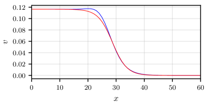
(a) Velocity

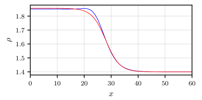
(b) Energy density

Figure 16: Comparison between a right-moving shock in (a) velocity and (b) energy density obtained from simulation data (blue line) and the shock profile predicted by section III.1 (red line) early on in a shock tube run. The viscosity of the run is $\eta=0.264$, and the parameter values used for the shock profile are $V_{+}=0.116$, $V_{m}=0$, and $x_{0}=28.7$, giving a shock velocity $u\approx 0.632$.

We see that the model matches the data quite well, apart from the crest of the shock, wherein there is a slight deviation from the value predicted by the model caused by the numerical scheme’s inability to precisely deal with sharp discontinuities. The strength of this effect depends on the initial rms velocity of the run, and the value of the viscosity, with large rms velocities and small viscosities leading to larger deviations and more oscillatory behaviour. This is demonstrated in Figure 17 where a right-moving shock profile has been plotted for runs with varying viscosity values. This effect can be reduced by using a higher order finite difference scheme, as can be seen in Figure 18, where a fourth order scheme has been used in performing the same run as in Figure 16a. By impacting the shock shape, higher order schemes also slightly change the shape of the energy spectrum at highwavenumbers and also, based on our tests, increase the amount of transverse power generated. Neither of these have a significant impact on the key results we have presented. Another aspect to consider is the conservation of the energy density $\left\langle\rho\right\rangle=\rho_{0}$, which is not by default taken into account when a central difference scheme is used. We have measured how well this conservation is fulfilled and we find that the largest deviations are obtained in the high Reynolds number runs. In run 9 the largest deviation for $\left\langle\rho\right\rangle/\rho_{0}$ from unity is 0.1, which is obtained only briefly at the start of the run, when the shocks are at their strongest, after about 4 shock formation times. The quantity remains mostly within 2.5% of the expected value and the deviations from it show a decreasing trend throughout the run after the initial phase. As these are the most extreme deviations and considering their small magnitude, we conclude that the energy density is conserved to a satisfactory level of accuracy even in the high Reynolds number case and thus the central difference scheme we have employed is expected to provide representative results for the set of runs we have featured in this paper.

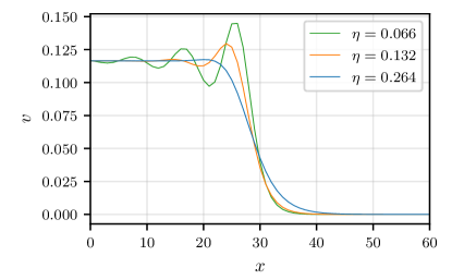
Figure 17: Shock profiles of different shock tube runs with varying values of shear viscosity after 6000 simulation time units.

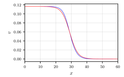
Figure 18: Figure 16a but a fourth order accurate finite difference scheme has been used in the run, improving the correspondence of the curves. All parameter values are the same apart from $x_{0}=29.0$.

The time evolution of the wave profile in a $\eta=0.264$ run has been plotted in Figure 19.

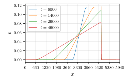
Figure 19: Evolution of the wave profile of a right-moving shock in the $\eta=0.264$ run. The profiles at various times have been shifted in $x$ to make the shocks overlap.

Over time the top of the wave profile gets narrower until a sawtooth form is reached. There is no decrease in the amplitude of the shock before this point. The opposite is true for the bottom of the wave profile, where it gets wider as time goes on. Using these properties, we have measured the velocity of the shock wave in this run and compared it to the value given by Equation (25) for the shock wave seen in the simulation. The chosen time window spans 6000 simulation time units, and is chosen near the start of the run in such a way that the wave profiles are not yet in the sawtooth phase, and there are no collisions between the right and left moving shock waves that could affect the shock speed. Since there is no decay in the amplitude and no change in the steepness of the shock, the propagation of a single point in the waveform can be measured in this interval, assuming a constant velocity. The value obtained from Equation (25) is found to be within 1% of th measured value.

Appendix B Runs and initial conditions

ID	$\alpha_{0}$	$\beta_{0}$	$\gamma$	$\beta_{0}-\alpha_{0}+1$	$k_{p}$	$A/V$	$B$	$\eta$	$\nu$	$|\delta|_{\text{max}}$	$t_{s}$	$\bar{v}$	Re
${\color[rgb]{0.12109375,0.46484375,0.70703125}1}$	$12$	$3$	$4$	$-8$	$0.100$	$64$	$0.5A$	$0.066$	$0$	$0.12$	$166$	$0.0761$	$10.9$
${\color[rgb]{1,0.49609375,0.0546875}2}$	$6$	$2$	$3$	$-3$	$0.035$	$128$	$1.0A$	$0.066$	$0$	$0.66$	$302$	$0.0768$	$20.2$
${\color[rgb]{0.171875,0.62890625,0.171875}3}$	$6$	$2$	$3$	$-3$	$0.035$	$128$	$1.0A$	$0$	$0.088$	$0.66$	$302$	$0.0768$	$20.2$
${\color[rgb]{0.83984375,0.15234375,0.15625}4}$	$9$	$3$	$3$	$-5$	$0.035$	$352$	$0.5A$	$0.066$	$0$	$0.14$	$301$	$0.0955$	$31.1$
${\color[rgb]{0.58203125,0.40234375,0.7421875}5}$	$20$	$4$	$5$	$-15$	$0.035$	$900$	$0.5A$	$0.066$	$0$	$0.12$	$532$	$0.0731$	$32.3$
${\color[rgb]{0.55078125,0.3359375,0.29296875}6}$	$10$	$4$	$2$	$-5$	$0.025$	$800$	$0.5A$	$0.066$	$0$	$0.08$	$300$	$0.1275$	$55.4$
${\color[rgb]{0.890625,0.46484375,0.76171875}7}$	$15$	$8$	$3$	$-6$	$0.009$	$17920$	$1.0A$	$0.066$	$0$	$0.50$	$625$	$0.1519$	$164.1$
${\color[rgb]{0.49609375,0.49609375,0.49609375}8}$	$7$	$4$	$2$	$-2$	$0.007$	$7840$	$1.0A$	$0.066$	$0$	$0.44$	$322$	$0.2201$	$177.4$
${\color[rgb]{0.73828125,0.7421875,0.1328125}9}$	$6$	$2$	$3$	$-3$	$0.007$	$15680$	$1.0A$	$0.066$	$0$	$0.27$	$643$	$0.1726$	$217.5$
${\color[rgb]{0.08984375,0.74609375,0.8125}10}$	$6$	$2$	$3$	$-3$	$0.007$	$15680$	$1.0A$	$0$	$0.088$	$0.27$	$643$	$0.1726$	$217.5$
${\color[rgb]{0.1875,0.1875,0.1875}11}$	$11$	$6$	$5$	$-4$	$0.006$	$89600$	$1.0A$	$0.066$	$0$	$0.61$	$595$	$0.1830$	$224.2$

Table 4: The initial parameter values for the spectral densities and some other quantities of interest in the $10080^{2}$-resolution runs used in this paper.

The runs have been performed using code written in Python with Cython [47] providing C-like performance in the most computationally demanding parts of the simulations, like in the evaluation of the spatial derivatives over arrays. The code is parallelised using MPI for Python [48] so that the computations can be distributed to multiple processor cores to provide further speed ups. NumPy [49] has been used for the computations involving arrays along with numexpr, which accelerates computations between arrays and optimises memory usage. The Runs have been conducted on CSC’s (Finnish IT center for science) supercomputer Puhti. All fits and numerical integrations used to obtain the results featured in this paper have been performed with SciPy [50], which is a Python library offering tools for scientific computing. The routines used are $\mathtt{curve\_fit}$ found in $\mathtt{scipy.optimize}$ for the fits, and $\mathtt{quad}$ found in $\mathtt{scipy.integrate}$ for the numerical integration. Numerical integration via $\mathtt{quad}$ is not however used in calculating quantities whose definitions contain integrals over the energy spectrum, such as the rms-velocities or the integral length scale in Equation (12). Instead, in those cases the integrals are discretised as sums over the squared Fourier arrays as

$$\int d^{2}k\rightarrow\frac{(2\pi)^{2}}{V}\sum\limits_{\bar{k}}\,,$$ (84)

where $V=N^{2}(\Delta x_{1})(\Delta x_{2})$. The routine from SciPy has only been used in the evaluation of the integrals in equations (38), (64) and (80).

The initial conditions are given in terms of the longitudinal and transverse spectral densities

$$P_{\parallel}(|\mathbf{k}|) =\frac{1}{V}\Big{(}|v_{x}^{\parallel}(\mathbf{k})|^{2}+|v_{y}^{\parallel}(\mathbf{k})|^{2}\Big{)}$$ (85)

$$P_{\perp}(|\mathbf{k}|) =\frac{1}{V}\Big{(}|v_{x}^{\perp}(\mathbf{k})|^{2}+|v_{y}^{\perp}(\mathbf{k})|^{2}\Big{)}$$ (86)

given in the form of Equation (10). The real space velocity components are then solved from these using the Fourier space projectors

$$v_{i}^{\perp}(\mathbf{k}) =(\delta_{ij}-\hat{k}_{i}\hat{k}_{j})v_{j}(\mathbf{k})$$ (87)

$$v_{i}^{\parallel}(\mathbf{k}) =\hat{k}_{i}\hat{k}_{k}v_{j}(\mathbf{k})$$ (88)

and by taking the inverse Fourier transforms of $v_{i}(\mathbf{k})$. Here $\delta_{ij}$ is the Kronecker delta, and the Einstein summation convention is applied. On the lattice, the unit vectors $\hat{k}_{i}$ are written in terms of the eigenvalues of the derivative operators as

$$\hat{k}_{i}=\frac{\sin(k_{i}\Delta x_{i})}{\sqrt{\sum\limits_{i}\sin^{2}(k_{i}\Delta x_{i})}}\,,$$ (89)

where $\Delta x_{i}$ is the lattice spacing in the direction of the $i$:th component. These projectors are also used to get the longitudinal energy spectra at non-initial times by applying them to the Fourier transformed velocity components. The Fourier transform algorithm utilised is the N-dimensional Fast Fourier Transform routine provided by NumPy. The spectrum $E_{\perp}(k)$ or $E_{\parallel}(k)$ is then obtained from the $N\times N$ sized arrays by radially averaging over circular rings of width $\Delta k$, which is the reciprocal lattice spacing. The averaging stops when the edges of the array are reached, meaning that the corner regions are ignored.

This paper contains results from 11 runs with a resolution of $10080^{2}$ whose initial conditions are listed in Table 4. In addition, there are a couple of $4080^{2}$ resolution runs that are used in plotting the contour plots of Figures 1 and 12 that use the same initial conditions as runs 2 and 9. The runs listed in the table are labelled from 1 to 11 in the order of increasing longitudinal Reynolds number. Columns 2-4 and 6-7 contain the initial parameter values for the longitudinal velocity spectral density given in Equation (10). The parameter $A$ has been scaled by dividing it by the volume $V$ to reduce its magnitude. The energy density is initialised in the same way as the velocity, and the initial density spectral density in all of the runs is the same, apart from the prefactor $A$ that is replaced by $B$, found in the 8th column of the table, given in terms of $A$. The 5th column shows the value of the initial high-$k$ power law in the energy spectrum.

The next two columns after the spectral parameters list the values of the shear viscosity $\eta$ and the bulk viscosity $\nu$. In the runs featured in this paper, all runs with shear viscosity use the value of $0.066$ and all runs with bulk viscosity use the value $0.088$. Finding a suitable value for the viscosity is a balancing act, as too large values either lead to no shocks forming at all, or to the formation of very weak and short lived shocks, whereas too low values give rise to significant instabilities and undesirable effects like the appearance of strong oscillations at the crest of the shocks. The bulk viscosity runs 3 and 10 use the same random seeds as runs 2 and 10, meaning they have the same initial waveforms both in velocity and density. All other runs use seeds that differ from each other.

The final four columns list some initial quantities measured from the initial conditions. The quantity $|\delta|_{\text{max}}$ is the largest value obtained by the fractional density perturbation $\delta\rho/\rho_{0}$ at the initial time, and $t_{s}$ is the shock formation time. The length of the runs in simulation time units is determined by it, as all of the runs are cut off after about 60 shock formation times. The final two columns list the initial root mean square velocity, and the longitudinal Reynolds number of the run, obtained using Equation (19). The cutoff parameter $k_{d}$ seen in the initial spectrum of equation 10 has the value of $1/\sqrt{5}$ in all runs.

The simulation code that has been used to create these runs can be found in Ref. [51]. Also included are the scripts used to initialise each of these runs. Non-related movies of longitudinal and transverse only runs produced with the simulation code can be found in Refs. [52, 53].

Appendix C Plots containing all of the runs

This section contains versions of Figures 8, 9, and 13 where curves from all runs found in table 4 are included in the plots. The runs are distinguishable from each other by the colours found in the ID column of the table.

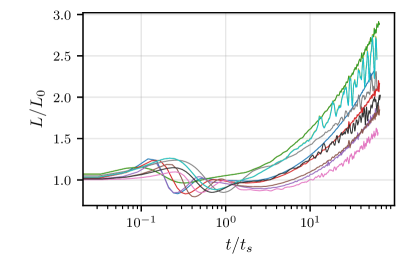
Figure 21: Figure 9 but all runs featured in table 4 are included.

References

- Abbott et al. [2016] B. P. Abbott et al. (LIGO Scientific, Virgo), Observation of Gravitational Waves from a Binary Black Hole Merger, Phys. Rev. Lett. 116, 061102 (2016), arXiv:1602.03837 [gr-qc] .
- Ricciardone [2017] A. Ricciardone, Primordial Gravitational Waves with LISA, J. Phys. Conf. Ser. 840, 012030 (2017), arXiv:1612.06799 [astro-ph.CO] .
- Christensen [2019] N. Christensen, Stochastic Gravitational Wave Backgrounds, Rept. Prog. Phys. 82, 016903 (2019), arXiv:1811.08797 [gr-qc] .
- Caprini and Figueroa [2018] C. Caprini and D. G. Figueroa, Cosmological Backgrounds of Gravitational Waves, Class. Quant. Grav. 35, 163001 (2018), arXiv:1801.04268 [astro-ph.CO] .
- Allen [1996] B. Allen, The Stochastic gravity wave background: Sources and detection, in Les Houches School of Physics: Astrophysical Sources of Gravitational Radiation (1996) pp. 373–417, arXiv:gr-qc/9604033 .
- Maggiore [2000] M. Maggiore, Gravitational wave experiments and early universe cosmology, Phys. Rept. 331, 283 (2000), arXiv:gr-qc/9909001 .
- Amaro-Seoane et al. [2017] P. Amaro-Seoane et al. (LISA), Laser Interferometer Space Antenna, (2017), arXiv:1702.00786 [astro-ph.IM] .
- Witten [1984] E. Witten, Cosmic Separation of Phases, Phys.Rev. D30, 272 (1984).
- Hogan [1986] C. J. Hogan, Gravitational radiation from cosmological phase transitions, Mon. Not. Roy. Astron. Soc. 218, 629 (1986).
- Kamionkowski et al. [1994] M. Kamionkowski, A. Kosowsky, and M. S. Turner, Gravitational radiation from first order phase transitions, Phys. Rev. D 49, 2837 (1994), arXiv:astro-ph/9310044 .
- Caprini et al. [2020] C. Caprini et al., Detecting gravitational waves from cosmological phase transitions with LISA: an update, JCAP 03, 024, arXiv:1910.13125 [astro-ph.CO] .
- Guth and Weinberg [1981] A. H. Guth and E. J. Weinberg, Cosmological Consequences of a First Order Phase Transition in the SU(5) Grand Unified Model, Phys. Rev. D23, 876 (1981).
- Steinhardt [1982] P. J. Steinhardt, Relativistic detonation waves and bubble growth in false vacuum decay, Phys.Rev. D25, 2074 (1982).
- Ignatius et al. [1994] J. Ignatius, K. Kajantie, H. Kurki-Suonio, and M. Laine, The growth of bubbles in cosmological phase transitions, Phys. Rev. D 49, 3854 (1994), arXiv:astro-ph/9309059 .
- Espinosa et al. [2010] J. R. Espinosa, T. Konstandin, J. M. No, and G. Servant, Energy Budget of Cosmological First-order Phase Transitions, JCAP 06, 028, arXiv:1004.4187 [hep-ph] .
- Mégevand and Ramírez [2018] A. Mégevand and S. Ramírez, Bubble nucleation and growth in slow cosmological phase transitions, Nucl. Phys. B 928, 38 (2018), arXiv:1710.06279 [astro-ph.CO] .
- Hindmarsh et al. [2014] M. Hindmarsh, S. J. Huber, K. Rummukainen, and D. J. Weir, Gravitational waves from the sound of a first order phase transition, Phys. Rev. Lett. 112, 041301 (2014), arXiv:1304.2433 [hep-ph] .
- Hindmarsh et al. [2015] M. Hindmarsh, S. J. Huber, K. Rummukainen, and D. J. Weir, Numerical simulations of acoustically generated gravitational waves at a first order phase transition, Phys. Rev. D 92, 123009 (2015), arXiv:1504.03291 [astro-ph.CO] .
- Hindmarsh et al. [2017] M. Hindmarsh, S. J. Huber, K. Rummukainen, and D. J. Weir, Shape of the acoustic gravitational wave power spectrum from a first order phase transition, Phys. Rev. D 96, 103520 (2017), [Erratum: Phys.Rev.D 101, 089902(E) (2020)], arXiv:1704.05871 [astro-ph.CO] .
- Hindmarsh and Hijazi [2019] M. Hindmarsh and M. Hijazi, Gravitational waves from first order cosmological phase transitions in the Sound Shell Model, JCAP 12, 062, arXiv:1909.10040 [astro-ph.CO] .
- Cutting et al. [2019] D. Cutting, M. Hindmarsh, and D. J. Weir, Vorticity, kinetic energy, and suppressed gravitational wave production in strong first order phase transitions, (2019), arXiv:1906.00480 [hep-ph] .
- L’vov et al. [1997] V. S. L’vov, Y. L’vov, A. C. Newell, and V. Zakharov, Statistical description of acoustic turbulence, Physical Review E 56, 390 (1997).
- L’vov et al. [2000] V. S. L’vov, Y. V. L’vov, and A. Pomyalov, Anisotropic spectra of acoustic turbulence, Phys. Rev. E 61, 2586 (2000), arXiv:chao-dyn/9905032 .
- Frisch and Bec [2000] U. Frisch and J. Bec, ’Burgulence’, in Les Houches 2000 Summer School: Session 74: New Trends in Turbulence (2000) arXiv:nlin/0012033 .
- Bec and Khanin [2007] J. Bec and K. Khanin, Burgers turbulence, Physics Reports 447, 1 (2007).
- Porter et al. [1992] D. Porter, A. Pouquet, and P. Woodward, A numerical study of supersonic turbulence, Theoretical and Computational Fluid Dynamics 4, 13 (1992).
- Kida and Orszag [1992] S. Kida and S. Orszag, Energy and spectral dynamics in decaying compressible turbulence, Journal of Scientific Computing 7, 1 (1992).
- Ducros et al. [1999] F. Ducros, V. Ferrand, F. Nicoud, C. Weber, D. Darracq, C. Gacherieu, and T. Poinsot, Large-eddy simulation of the shock/turbulence interaction, Journal of Computational Physics 152, 517 (1999).
- Pen and Turok [2016] U.-L. Pen and N. Turok, Shocks in the Early Universe, Phys. Rev. Lett. 117, 131301 (2016), arXiv:1510.02985 [astro-ph.CO] .
- Roper Pol et al. [2020] A. Roper Pol, S. Mandal, A. Brandenburg, T. Kahniashvili, and A. Kosowsky, Numerical simulations of gravitational waves from early-universe turbulence, Phys. Rev. D 102, 083512 (2020), arXiv:1903.08585 [astro-ph.CO] .
- Brandenburg et al. [1996] A. Brandenburg, K. Enqvist, and P. Olesen, Large scale magnetic fields from hydromagnetic turbulence in the very early universe, Phys. Rev. D 54, 1291 (1996), arXiv:astro-ph/9602031 .
- Arnold et al. [2006] P. B. Arnold, C. Dogan, and G. D. Moore, The Bulk Viscosity of High-Temperature QCD, Phys. Rev. D 74, 085021 (2006), arXiv:hep-ph/0608012 .
- Hewitt and Hewitt [1979] E. Hewitt and R. E. Hewitt, The gibbs-wilbraham phenomenon: An episode in fourier analysis, Archive for History of Exact Sciences 21, 129 (1979).
- Burgers [1948] J. Burgers, A mathematical model illustrating the theory of turbulence, Advances in Applied Mechanics 1, 171 (1948).
- Kadomtsev and Petviashvilil [1973] B. Kadomtsev and V. Petviashvilil, Dokl. Akad. Nauk SSSR 208, 794 (1973).
- Kuznetsov and Krasnoselskikh [2008] E. Kuznetsov and V. Krasnoselskikh, Anisotropic spectra of acoustic type turbulence, Physics of Plasmas 15, 062305 (2008), https://doi.org/10.1063/1.2928160 .
- Erdélyi et al. [1954] A. Erdélyi, W. Magnus, F. Oberhetinger, and F. Tricomi, Tables of integral transforms, Vol. 2 (McGraw-Hill, 1954) Chap. 13.
- Saffman [1971] P. G. Saffman, On the spectrum and decay of random two‐dimensional vorticity distributions at large reynolds number, Studies in Applied Mathematics 50, 10.1002/sapm1971504377 (1971).
- Lesieur [2008] M. Lesieur, Turbulence in Fluids, Fluid Mechanics and Its Applications (Springer Netherlands, 2008).
- Olesen [1997] P. Olesen, On inverse cascades in astrophysics, Phys. Lett. B 398, 321 (1997), arXiv:astro-ph/9610154 .
- Brandenburg and Kahniashvili [2017] A. Brandenburg and T. Kahniashvili, Classes of hydrodynamic and magnetohydrodynamic turbulent decay, Phys. Rev. Lett. 118, 055102 (2017), arXiv:1607.01360 [physics.flu-dyn] .
- Kosowsky et al. [2002] A. Kosowsky, A. Mack, and T. Kahniashvili, Gravitational radiation from cosmological turbulence, Phys. Rev. D 66, 024030 (2002), arXiv:astro-ph/0111483 .
- Gogoberidze et al. [2007] G. Gogoberidze, T. Kahniashvili, and A. Kosowsky, The Spectrum of Gravitational Radiation from Primordial Turbulence, Phys. Rev. D 76, 083002 (2007), arXiv:0705.1733 [astro-ph] .
- Caprini et al. [2008] C. Caprini, R. Durrer, and G. Servant, Gravitational wave generation from bubble collisions in first-order phase transitions: An analytic approach, Phys. Rev. D 77, 124015 (2008), arXiv:0711.2593 [astro-ph] .
- Caprini et al. [2009a] C. Caprini, R. Durrer, and G. Servant, The stochastic gravitational wave background from turbulence and magnetic fields generated by a first-order phase transition, JCAP 12, 024, arXiv:0909.0622 [astro-ph.CO] .
- Caprini et al. [2009b] C. Caprini, R. Durrer, T. Konstandin, and G. Servant, General Properties of the Gravitational Wave Spectrum from Phase Transitions, Phys. Rev. D 79, 083519 (2009b), arXiv:0901.1661 [astro-ph.CO] .
- Behnel et al. [2011] S. Behnel, R. Bradshaw, C. Citro, L. Dalcin, D. S. Seljebotn, and K. Smith, Cython: The best of both worlds, Computing in Science Engineering 13, 31 (2011).
- Dalcín et al. [2005] L. Dalcín, R. Paz, and M. Storti, Mpi for python, Journal of Parallel and Distributed Computing 65, 1108 (2005).
- Harris et al. [2020] C. R. Harris et al., Array programming with NumPy, Nature 585, 357 (2020).
- Virtanen et al. [2020] P. Virtanen et al., SciPy 1.0: Fundamental Algorithms for Scientific Computing in Python, Nature Methods 17, 261 (2020).
- Dahl [2021a] J. Dahl, Simulation code for fluids in two dimensions (2021a).
- Dahl [2021b] J. Dahl, Simulation code for fluids in two dimensions - density and velocity movies (2021b).
- Dahl [2021c] J. Dahl, Simulation code for fluids in two dimensions - vorticity movie (2021c).