Astrophysical magnetic fields and nonlinear dynamo theory

Abstract

The current understanding of astrophysical magnetic fields is reviewed, focusing on their generation and maintenance by turbulence. In the astrophysical context this generation is usually explained by a self-excited dynamo, which involves flows that can amplify a weak ‘seed’ magnetic field exponentially fast. Particular emphasis is placed on the nonlinear saturation of the dynamo. Analytic and numerical results are discussed both for small scale dynamos, which are completely isotropic, and for large scale dynamos, where some form of parity breaking is crucial. Central to the discussion of large scale dynamos is the so-called alpha effect which explains the generation of a mean field if the turbulence lacks mirror symmetry, i.e. if the flow has kinetic helicity. Large scale dynamos produce small scale helical fields as a waste product that quench the large scale dynamo and hence the alpha effect. With this in mind, the microscopic theory of the alpha effect is revisited in full detail and recent results for the loss of helical magnetic fields are reviewed.

and

1 Introduction

Magnetic fields are ubiquitous in the universe. Our most immediate encounter with magnetic fields is the Earth’s field. This field is not only useful for navigation, but it also protects us from hazardous cosmic ray particles. Magnetic fields play an important role in various branches of astrophysics. They are particularly important for angular momentum transport, without which the sun and similar stars would not spin as slowly as they do today [1]. Magnetic fields are responsible for the loops and arcades seen in X-ray images of the sun and in heating the coronae of stars with outer convection zones [2]. They play a crucial role in driving turbulence in accretion discs providing the stresses needed for accretion. Large scale fields in these discs are also thought to be involved in driving jets. A field permeating a rotating black hole probably provides one of the most efficient ways of extracting energy to power the jets from active galactic nuclei. Magnetic fields with micro-gauss strength and coherence scales of order several kilo parsecs are also observed in nearby galaxies and perhaps even in galaxies which have just formed. The magnetic field strength in galactic spiral arms can be up to 30 microgauss (e.g. in M51). Fields of order several micro-gauss and larger, with even larger coherence scales, are seen in clusters of galaxies. To understand the origin of magnetic fields in all these astrophysical systems is a problem of great importance.

The universe may not have begun magnetized. There are various processes such as battery effects, which can lead to a weak magnetic field, from zero initial fields. Most of these batteries lead to field strengths much weaker than the observed field, as will be discussed further in Section 3.9. So some way of amplifying the field is required. This is probably accomplished by the conversion of kinetic energy into magnetic energy, a process generally referred to as a dynamo; see Ref. [3] for a historic account. Some basic principles of dynamos are well understood from linear theory, but virtually all astrophysical dynamos are in a regime where the field is dynamically important, and kinematic theory is invalid. In recent years our understanding of nonlinear properties of dynamos has advanced rapidly. This is partly due to new high resolution numerical simulations which have also triggered further developments in analytic approaches. An example is the resistively slow saturation phase of dynamos with helicity that was first seen in numerical simulations [4], which then led to the development of a dynamical quenching model [5, 6, 7, 8]; see Section 9.3. The dynamical quenching model was actually developed much earlier [9], but it was mostly applied in order to explain chaotic behavior of the solar cycle [10, 11, 12]. Another example is the so-called small scale dynamo whose theory goes back to the early work of Kazantsev [13]; see Section 5.2. Again, only in recent years, with the advent of fast computers allowing high Reynolds number simulations of hydromagnetic turbulence, the community became convinced of the reality of the small scale dynamos. This in turn has triggered further advances in the theoretical understanding this problem, especially the nonlinear stages. Also quite recent is the realization that the small scale dynamo is much harder to excite when, for fixed resistivity, the viscosity is decreased (i.e. the magnetic Prandtl number is less than unity) so that the magnetic field is driven by a rough velocity field (Section 5.5).

Although there have been a number of excellent reviews about dynamo theory and comparisons with observations of astrophysical magnetic fields [14, 15, 16, 17, 18, 19, 20, 21, 22], there have been many crucial developments just over the past few years involving primarily magnetic helicity. It has now become clear that nonlinearity in large scale dynamos is crucially determined by the magnetic helicity evolution equation. At the same time, magnetic helicity has also become highly topical in observational solar physics, as is evidenced by a number of recent specialized meetings on exactly this topic [23]. Magnetic helicity emerges therefore as a new tool in both observational as well as in theoretical studies of astrophysical magnetohydrodynamics (MHD). This review discusses the details of why this is so, and how magnetic helicity can be used to constrain dynamo theory and to explain the behavior seen in recent simulations of dynamos in the nonlinear, high magnetic Reynolds number regime.

We also review some basic properties and techniques pertinent to mean field (large scale) dynamos (Section 10), so that newcomers to the field can gain deeper insight and are able to put new developments into perspective. In particular, we discuss a simplistic form of the so-called tau approximation that allows the calculation of mean field turbulent transport coefficients in situations where the magnetic fluctuations strongly exceed the magnitude of the mean field. This is when the quasilinear theory (also known as first order smoothing or second order correlation approximation) breaks down. We then lead to the currently intriguing question of what saturates the dynamo and why so much can be learned by rather simple considerations in terms of magnetic helicity.

In turbulent fluids, the generation of large scale magnetic fields is generically accompanied by the more rapid growth of small scale fields. The growing Lorentz force due to these fields can back-react on the turbulence to modify the mean field dynamo coefficients. A related topic of great current interest is the non helical small scale dynamo, and especially its nonlinear saturation. This could also be relevant for explaining the origin of cluster magnetic fields. These topics are therefore reviewed in the light of recent advances using both analytic tools as well as high resolution simulations (Section 5).

There are obviously many topics that have been left out, because they touch upon nonlinear dynamo theory only remotely. Both hydrodynamic and magnetohydrodynamic turbulence are only discussed in their applications, but there are many fundamental aspects that are interesting in their own right; see the text books by Frisch [24] and Biskamp [25] and the work by Goldreich and Sridhar [26]; for a recent review see Ref. [27]. Another broad research area that has been left out completely is magnetic reconnection and low beta plasmas. Again, we can here only refer to the text book by Priest and Forbes [28]. More close connections exist with hydrodynamic mean field theory relevant for explaining differential rotation in stars [29]. Even many of the applications of dynamo theory are outlined only rather broadly, but again, we can refer to a recent text book by Rüdiger and Hollerbach [30] where many of these aspects are addressed.

We begin in the next section with some observational facts that may have a chance in finding an explanation in terms of dynamo theory within the not too distant future. We then summarize some useful facts of basic MHD, and also discuss briefly battery effects to produce seed magnetic fields. Some general properties of dynamos are discussed in Section 4. These two sections are relatively general and can be consulted independently of the remainder. We then turn to small scale dynamos in Section 5. Again, this section may well be read separately and does not contain material that is essential for the remaining sections. The main theme of large scale dynamos is extensively covered in Sections 6–10. Finally, in Section 11 we discuss some applications of these ideas to various astrophysical systems. Some final reflections on outstanding issues are given in Section 12.

2 Magnetic field observations

In this section we discuss properties of magnetic fields observed in various astrophysical settings. We focus specifically on aspects that are believed to be important for nonlinear dynamo theory and its connection with magnetic helicity. We begin with a discussion of the solar magnetic field, which consists of small scale and large scale components. The typical length scale associated with the large scale field is the width of the toroidal flux belts with the same polarity which is around $30^{\circ}$ in latitude, corresponding to about $300\,{\rm Mm}$ ($1\,{\rm Mm}=1000\,{\rm km}$). The pressure scale height at the bottom of the convection zone is about $50\,{\rm Mm}$, and all scales shorter than that may be associated with the small scale field.

The theory of the large scale component has been most puzzling, while the small scale field could always be explained by turbulence and convection shredding and concentrating the field into isolated flux bundles. The simultaneous involvement of a so-called small scale dynamo may provide another source for the small scale field, which needs to be addressed. We begin by outlining the observational evidence for large scale fields in the sun and in stars, and discuss then the evidence for magnetic fields in accretion discs and galaxies, as well as galaxy clusters.

2.1 Solar magnetic fields

The sun has a magnetic field that manifests itself in sunspots through Zeeman splitting of spectral lines [31]. It has long been known that the sunspot number varies cyclically with a period between 7 and 17 years. The longitudinally averaged component of the radial magnetic field of the sun [32, 33] shows a markedly regular spatio-temporal pattern where the radial magnetic field alternates in time over the 11 year cycle and also changes sign across the equator (Fig. 2.1). One can also see indications of a migration of the field from mid latitudes toward the equator and the poles. This migration is also well seen in a sunspot diagram, which is also called a butterfly diagram, because the pattern formed by the positions of sunspots in time and latitude looks like a sequence of butterflies lined up along the equator (Fig. 2.2).

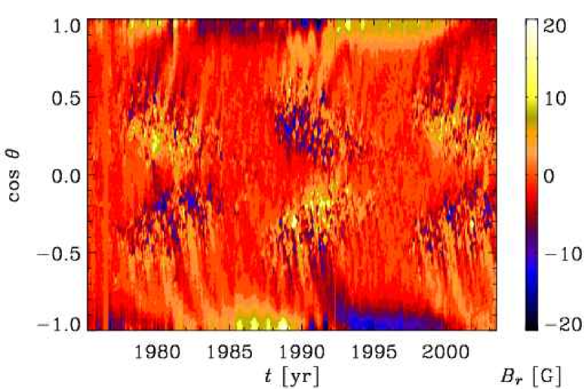
Figure 2.1: Longitudinally averaged radial component of the observed solar magnetic field as a function of cos(colatitude) and time. Dark (blue) shades denote negative values and light (yellow) shades denote positive values. Note the sign changes both in time and across the equator (courtesy of R. Knaack).

At the solar surface the azimuthally averaged radial field is only a few gauss ($1\,{\rm G}=10^{-4}\,\mbox{Tesla}$). This is rather weak compared with the peak magnetic field in sunspots of about $2\,{\rm kG}$. In the bulk of the convection zone, because of differential rotation, the magnetic field is believed to point mostly in the azimuthal direction, and it is probably much larger near the bottom of the convection zone due to an effect known as downward pumping (Section 6.4).

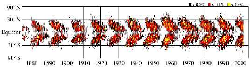
Figure 2.2: Solar butterfly diagram showing the sunspot number in a space-time diagram. Note the migration of sunspot activity from mid-latitudes toward the equator (courtesy of D. N. Hathaway).

2.1.1 Estimates of the field strength in the deeper convection zone

In the bulk of the solar convection zone the thermal energy transport is reasonably well described by mixing length theory [34]. This theory yields a rough estimate for the turbulent rms velocity which is around $u_{\rm rms}=20\,{\rm m}\,{\rm s}^{-1}$ near the bottom of the solar convection zone. With a density of about $\rho=0.2\,{\rm g}\,{\rm cm}^{-3}$ this corresponds to an equipartition field strength of about $3\,{\rm kG}$. (The equipartition field strength is here defined as $B_{\rm eq}=\sqrt{\mu_{0}\rho}\,u_{\rm rms}$, where $\mu_{0}$ is the magnetic permeability.)

A similar estimate is obtained by considering the total (unsigned) magnetic flux that emerges at the surface during one cycle. This argument is dubious, because one has to make an assumption about how many times the flux tubes in the sun have emerged at the solar surface. Nevertheless, the notion of magnetic flux (and especially unsigned flux) is rather popular in solar physics, because this quantity is readily accessible from solar magnetograms. The total unsigned magnetic flux is roughly estimated to be $10^{24}\,{\rm Mx}$. Distributed over a meridional cross-section of about $500\,{\rm Mm}$ in the latitudinal direction and about $50\,{\rm Mm}$ in radius (i.e. the lower quarter of the convection zone) yields a mean field of about $4\,{\rm kG}$, which is in fair agreement with the equipartition estimate above. This type of argumentation has first been proposed in an early paper by Galloway & Weiss [35].

Another type of estimate concerns not the mean field but rather the peak magnetic field in the strong flux tubes. Such tubes are believed to be ‘stored’ either just below or at the bottom of the convection zone. By storage one means that the field survives reasonably undisturbed for a good fraction of the solar cycle and evolves mostly under the amplifying action of differential rotation. Once such a flux tube becomes buoyant in one section of the tube it rises, expands and becomes tilted relative to the azimuthal direction owing to the Coriolis force. Calculations based on the thin flux tube approximation [36] predict field strengths of about $100\,{\rm kG}$ that are needed in order to produce the observed tilt angle of bipolar sunspots near the surface [37].

The systematic variation of the global field of the sun is important to understand both for practical reasons, e.g. for space weather forecasts, and for theoretical reasons because the solar field is a prime example of what we call large scale dynamo action. The 11 year cycle of the sun is commonly explained in terms of $\alpha\Omega$ dynamo theory (Sections 6.5 and 11.2), but this theory faces a number of problems that will be discussed later. Much of the resolution of these problems focuses around magnetic helicity. This has become a very active research field in its own right. Here we discuss the observational evidence.

2.1.2 Magnetic helicity of the solar field

Magnetic helicity studies have become an important observational tool to quantify the complexity of the sun’s magnetic field. Examples of complex magnetic structures being ejected from the solar surface are shown in Fig. 2.3. For a series of reviews covering the period until 1999 see Ref. [38]. The significance of magnetic helicity for understanding the nonlinear dynamo has only recently been appreciated. Here we briefly review some of the relevant observational findings.

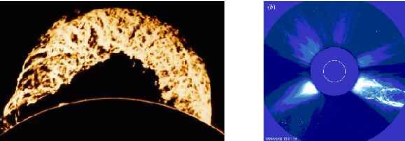
Figure 2.3: The famous “Grand daddy” prominence of 4 June 1946 (left) and a big coronal mass eruption of 2 June 1998 from the LASCO coronograph on board the SOHO satellite (right). Note the complexity of the ejected structures, being suggestive of helical nature. Courtesy of the SOHO consortium. SOHO is a project of international cooperation between ESA and NASA.

The only information about the magnetic helicity of the sun available to date is from surface magnetic fields, and these data are necessarily incomplete. Nevertheless, some systematic trends can be identified.

Vector magnetograms of active regions show negative (positive) current helicity in the northern (southern) hemisphere [39, 40, 41, 42]. From local measurements one can only obtain the current helicity density, so nothing can be concluded about magnetic helicity, which is a volume integral. As we shall show later (Section 3.7), under the assumption of isotropy, the spectra of magnetic and current helicity are however simply related by a wavenumber squared factor. This implies that the signs of current and magnetic helicities agree if they are determined in a sufficiently narrow range of length scales. We return to this issue in Section 9.4.

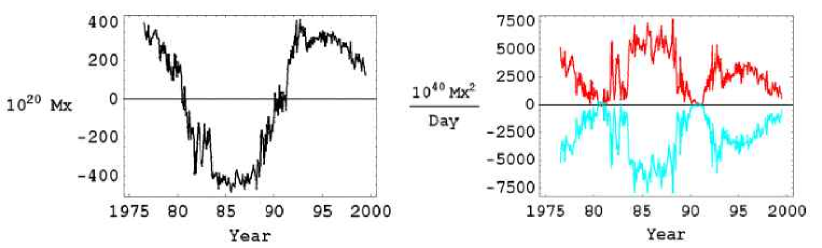
Figure 2.4: Net magnetic flux through the solar surface at the northern hemisphere (left hand panel) and magnetic helicity flux for northern and southern hemispheres (right hand panel, lower and upper curves, respectively). Adapted from Berger and Ruzmaikin [43].

Berger and Ruzmaikin [43] have estimated the flux of magnetic helicity from the solar surface using magnetograms. They discussed the $\alpha$ effect and differential rotation as the main agents facilitating the loss of magnetic helicity. Their results indicate that the flux of magnetic helicity due to differential rotation and the observed radial magnetic field component is negative (positive) in the northern (southern) hemisphere, and of the order of about $10^{46}\,{\rm Mx}^{2}$ integrated over the 11 year cycle; see Fig. 2.4.

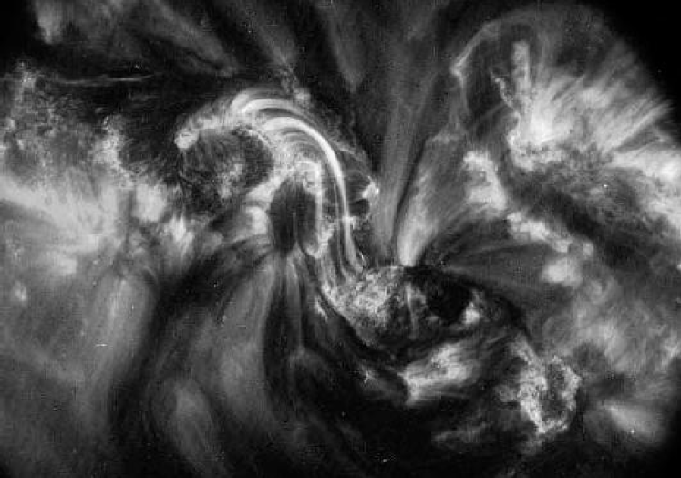
Figure 2.5: X-ray image at $195\,$Å  showing an N-shaped sigmoid (right-handed writhe) of the active region NOAA AR 8668 at the northern hemisphere (1999 August 21 at 18:51 UT). Adapted from Gibson et al. [47].

Chae [44] estimated the magnetic helicity flux based on counting the crossings of pairs of flux tubes. Combined with the assumption that two nearly aligned flux tubes are nearly parallel, rather than anti-parallel, his results again suggest that the magnetic helicity is negative (positive) in the northern (southern) hemisphere. The same sign distribution was also found by DeVore [45] who considered magnetic helicity generation by differential rotation. He finds that the magnetic helicity flux integrated over an 11 year cycle is about $10^{46}\,{\rm Mx}^{2}$ both from active regions and from coronal mass ejections. Thus, the sign agrees with that of the current helicity obtained using vector magnetograms. More recently, Démoulin et al. [46] showed that oppositely signed twist and writhe from shear are able to largely cancel, producing a small total magnetic helicity. This idea of a bi-helical field is supported further by studies of sigmoids [47]: an example is Fig. 2.5, which shows a TRACE image of an N-shaped sigmoid (right-handed writhe) with left-handed twisted filaments of the active region NOAA AR 8668, which is typical of the northern hemisphere. This observation is quite central to our new understanding of nonlinear dynamo theory [48, 49] and will be addressed in more detail below (Section 9.6.2).

2.1.3 Active longitudes

An important piece of information about the sun concerns the so-called active longitudes. These are longitudes where magnetic activity re-occurs over long durations, exceeding even the length of the solar cycle [50, 51, 52, 53]. On shorter time scales of about half a year, the angular velocity of active longitudes depends on the phase during the solar cycle, and hence on the latitude of their occurrence. At the beginning of the cycle, when new flux appears at high latitudes ($\pm 30^{\circ}$ latitude), the rotation rate of these active longitudes is about $446\,{\rm nHz}$. At this latitude the rotation rate of $446\,{\rm nHz}$ agrees with the value inferred from helioseismology at the fractional radius $r/R_{\odot}\approx 0.95$; see Fig. 2.6.

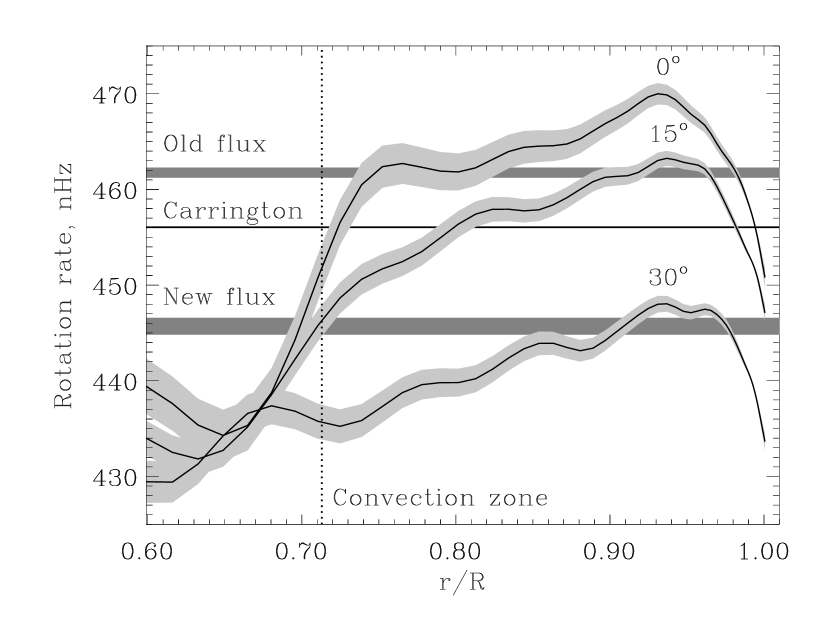
Figure 2.6: Radial profiles of the internal solar rotation rate, as inferred from helioseismology (sidereal, i.e. in a fixed frame). The rotation rate of active zones at the beginning of the cycle (at $\approx 30^{\circ}$ latitude) and near the end (at $\approx 4^{\circ}$) is indicated by horizontal bars, which intersect the profiles of rotation rate at $r/R_{\odot}\approx 0.97$. For orientation, the conventionally defined Carrington rotation period of 27.3 days (synodic value, corresponding to $424\,{\rm nHz}$) has been translated to the sidereal value of $456\,{\rm nHz}$. Courtesy of Benevolenskaya et al. [54].

If this magnetic activity were to come from the bottom of the convection zone at $r/R_{\odot}\approx 0.7$, where the rotation rate is around $435\,{\rm nHz}$, it would be by $11\,{\rm nHz}$ too slow (Fig. 2.6). After half a year, the corresponding regions at $r/R_{\odot}\approx 0.7$ and 0.95 would have drifted apart by $62^{\circ}$. Thus, if the active longitudes were to be anchored at $r/R_{\odot}\approx 0.7$, they could not be connected with matter at this latitude; instead they would need to be mapped to a lower latitude of about $15^{\circ}$, where the rotation rate at $r/R_{\odot}\approx 0.7$ agrees with the value of $446\,{\rm nHz}$ found for the active longitudes at $30^{\circ}$ latitude. Alternatively, they may simply be anchored at a shallower depth corresponding to $r/R_{\odot}\approx 0.95$, where the rotation rate of these active longitudes agrees with the helioseismologically inferred value. Similar considerations apply also to the rotation rate of old flux that occurs at about $\pm 4^{\circ}$ latitude. However, here the anchoring depth is ambiguous and could be either $r/R_{\odot}\approx 0.97$ or in the range 0.75…0.80. The rather unconventional suggestion of a shallow anchoring depth [55] will be addressed further at the end of Section 11.2.8.

2.2 Magnetic fields of late type stars

Looking at other stars is important for appreciating that the solar dynamo is not unique and just one particular example of a dynamo that happened to be a cyclic one. In fact, we now know that all stars with outer convection zones (usually referred to as ‘late-type stars’) have magnetic fields whose strength tends to increase with their angular velocity. Some very young stars (e.g. T Tauri stars) have average field strengths of about $2\,{\rm kG}$ [56]. These stars are fully convective and their field varies in a more erratic fashion. Cyclic variations are known to exist only for stars with colors $B-V$ in the range 0.57 and 1.37, i.e. for spectral types between G0 and K7 [57]. Some examples of the time traces are shown in Fig. 2.7. The sun’s color is 0.66, being close to the upper (bluer) end of the mass range where stars show cyclic activity. For the stars in this mass range there exists an empirical relation between three important parameters. One is the inverse Rossby number, $\mbox{Ro}^{-1}\equiv 2\Omega\tau_{\rm turnover}$, where $\tau_{\rm turnover}\approx\ell/u_{\rm rms}$ is the turnover time of the convection, estimated in terms of the mixing length, $\ell$, and the rms velocity of the convection, $u_{\rm rms}$. The second parameter is the ratio of cycle to rotation frequency, $\omega_{\rm cyc}/\Omega$, where $\omega_{\rm cyc}=2\pi/P_{\rm cyc}$ and $P_{\rm cyc}$ is the cycle period ($\approx 11$ years for the sun, but ranging from 7 to 21 years for other stars). The third parameter is the ratio of the mean chromospheric Calcium H and K line emission to the bolometric flux, $\langle R_{\rm HK}^{\prime}\rangle$, which can be regarded as a proxy of the normalized magnetic field strength, with $\langle R_{\rm HK}^{\prime}\rangle\propto(|\langle\bm{B}\rangle|/B_{\rm eq})^{\kappa}$ and $\kappa\approx 0.47$; see Ref. [58]. These three parameters are related to each other by approximate power laws,

$$\omega_{\rm cyc}/\Omega\approx c_{1}\mbox{Ro}^{-\sigma},\quad\omega_{\rm cyc}/\Omega\approx c_{2}\langle R_{\rm HK}^{\prime}\rangle^{\nu}\quad\langle R_{\rm HK}^{\prime}\rangle\approx c_{3}\mbox{Ro}^{-\mu},$$ (2.1)

where $c_{1}=c_{2}c_{3}^{\nu}$ and $\sigma=\mu\nu$. It turns out that the slopes $\sigma$ and $\nu$ are positive for active (A) and inactive (I) stars and that both groups of stars fall on distinct branches with $\sigma_{\sf A}\approx 0.46$ and $\nu_{\sf A}\approx 0.85$ for active stars and $\sigma_{\sf I}\approx 0.48$ and $\nu_{\sf I}\approx 0.72$ for inactive stars [59]. Since $\sigma$ and $\nu$ are obtained from separate fits, there is of course no guarantee that the relation $\sigma=\mu\nu$ will be obeyed by the data obtained from separate fits.

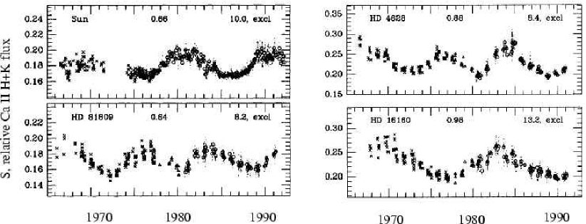
Figure 2.7: Time traces of the relative Calcium H and K line emission, $S$, for 4 stars (including the sun) with oscillatory activity behavior between the years 1966 and 1992 (adapted from Baliunas et al. [57])

Figure 2.8: Mutual correlations between the three quantities $\omega_{\rm cyc}/\Omega$, $\mbox{Ro}^{-1}$, and $\langle R_{\rm HK}^{\prime}\rangle$. Note the two distinct branches, separate by a factor of about 6 in the ratio $\omega_{\rm cyc}/\Omega$, with positive slope in the first two panels. The numbers and letters in the plots are abbreviations for specific active and inactive stars, respectively (adapted from Ref. [59], where also a key with the abbreviations of all stars is given). The values of $\sigma$, $\nu$, and $\mu$, given in the titles of the three plots, are obtained from three independent plots and hence do not obey the relation $\sigma=\mu\nu$.

In Fig. 2.8 we present scatter plots showing the mutual correlations between each of the three quantities for all cyclic stars whose parameters have been detected with quality parameters that were labeled [57] as ‘good’ and ‘excellent’. Plots similar to the third panel of Fig. 2.8 have also been produced for other activity proxies [60]. This work shows that there is a relation between activity proxy and inverse Rossby number not only for stars with magnetic activity cycles, but for all late type stars with outer convection zones – even when the stars are members of binaries [61].

The fact that the cycle frequency depends in a systematic fashion on either $\mbox{Ro}^{-1}$ or on $\langle R_{\rm HK}^{\prime}\rangle$ suggests that for these stars the dynamo has a rather stable dependence on the input parameters. What is not well understood, however, is the slope $\sigma\approx 0.5$ in the relation $\omega_{\rm cyc}/\Omega\sim\mbox{Ro}^{-\sigma}$, and the fact that there are two distinct branches. We note that there is also evidence for a third branch for even more active (‘superactive’) stars, but there the exponent $\sigma$ is negative [61]. Standard dynamo theory rather predicts that $\sigma$ is always negative [62]. We return to a possible interpretation of the exponent $\sigma$ and the origin of the different branches in Section 11.3.2.

2.3 Magnetic fields in accretion discs

Gaseous discs spinning around some central object are frequently found in various astrophysical settings, for example around young stars, stellar mass compact objects (white dwarfs, neutron stars, or black holes), or in supermassive ($10^{7}-10^{9}M_{\odot}$) black holes that have been found or inferred to exist in virtually all galaxies.

Explicit evidence for magnetic fields in discs is sparse: magnetization of meteorites that were formed in the disc around the young sun [63] or proxies of magnetic activity such as $H_{\beta}$ line emission from discs in binary stars [64]. A direct search for Zeeman-induced splitting of the maser lines in the accretion disc of the Seyfert II galaxy NGC 4258 has resulted in upper limits of $<50\,{\rm mG}$ for the toroidal component of the $B$ field at a distance of about 0.2 pc from the central black hole [65]. Faraday rotation measure (RM) maps of the central parsecs of quasars and radio galaxies hosting relativistic jets [66] also reveal that the medium on parsec scales surrounding AGNs could be significantly magnetized [67].

There are two strong theoretical reasons, however, why accretion discs should be magnetized. First, discs are often formed in an already magnetized environment. This is particularly clear for protostellar discs whose axes of rotation are often aligned with the direction of the ambient field [68]. Second, discs with weak ambient fields are unstable to the magnetorotational instability [69, 70] which, coupled with the dynamo instability, can leads to equipartition field strengths. In the case of protostellar discs, however, it is possible that the magnetorotational instability only worked in its early stages. At later stages, the parts of the disc near the midplane and at $\sim 1\,{\rm AU}$ distance from the central state may have become too cold and almost neutral, so these parts of the disc may then no longer be magnetized [71].

Many accretion discs around black holes are quite luminous. For example, the luminosity of active galactic nuclei can be as large as 100 times the luminosity of ordinary galaxies. Here, magnetic fields provide the perhaps only source of an instability that can drive the turbulence and hence facilitate the conversion of potential energy into thermal energy or radiation. In discs around active galactic nuclei the magnetic field may either be dragged in from large radii or it may be regenerated locally by dynamo action.

The latter possibility is particularly plausible in the case of discs around stellar mass black holes. Simulations have been carried out to understand this process in detail; see Section 11.4. Magnetic fields may also be crucial for driving outflows from discs. In many cases these outflows may be collimated by the ambient magnetic field to form the observed narrow jets [72].

2.4 Galactic magnetic fields

Galaxies and clusters of galaxies are currently the only astrophysical bodies where a large scale magnetic field can be seen inside the body itself. In the case of stars one only sees surface manifestations of the field. Here we describe the structure and magnitude of galactic fields.

2.4.1 Synchrotron emission from galaxies

Magnetic fields in galaxies are mainly probed using radio observations of their synchrotron emission. Excellent accounts of the current observational status can be found in the various reviews by Beck [73, 74, 75, 76] and references therein. We summarize here those aspects which are relevant to our discussion of galactic dynamos. Some earlier reviews of the observations and historical perspectives can be found in Refs [15, 16, 17, 77]. A map of the total synchrotron intensity allows one to estimate the total interstellar magnetic field in the plane of the sky (averaged over the volume sampled by the telescope beam). The synchrotron emissivity also depends on the number density of relativistic electrons, and so some assumption has to be made about its density. One generally assumes that the energy densities of the field and particles are in equipartition. (Specifically, equipartition is assumed to hold between magnetic fields and relativistic protons so that the proton/electron ratio enters as another assumption, with 100 taken as a standard value.) In our Galaxy the accuracy of the equipartition assumption can be tested, because we have independent measurements of the local cosmic-ray electron energy density from direct measurements and about the cosmic-ray proton distribution from $\gamma$-ray data. The combination of these with the strength of the radio continuum synchrotron emission gives a local strength of the total magnetic field of $6\pm 1\,\mu{\rm G}$ [78], which is almost the same value as that derived from energy equipartition [74].

The mean equipartition strength of the total magnetic field for a sample of 74 spiral galaxies is $\langle B_{\rm tot}\rangle=9\,\mu{\rm G}$ [73, 79]. The total field strength ranges from $\langle B_{\rm tot}\rangle\sim 4\,\mu{\rm G}$, in radio faint galaxies like M31 and M33 to $\langle B_{\rm tot}\rangle\sim 15\,\mu{\rm G}$ in grand design spiral galaxies like M51, M83 and NGC 6946 [76]. The strength of the total field in the inner spiral arms of M51 is about $30\,\mu{\rm G}$.

Synchrotron radiation is intrinsically highly linearly polarized, by $70$–$75\%$ in a completely regular magnetic field [80]. The observable polarization is however reduced due to a number of reasons. First the magnetic field usually has a tangled component which varies across the telescope beam (geometrical depolarization); second due to Faraday depolarization in the intervening medium and third because some part of the radio emission arises due to thermal continuum emission, rather than synchrotron emission. A map of the polarized intensity and polarization angle then gives the strength and structure of the ordered field, say $\overline{B}$ in the plane of the sky. Note that polarization can also be produced by any random field, which is compressed or stretched in one dimension (i.e. an anisotropic field which incoherently reverses its direction frequently) [81, 82]. So, to make out if the field does really have large scale order one needs also a map of Faraday rotation measures (RMs), as this will show large scale coherence only for ordered fields. Such a map also probes the strength and direction of the average magnetic field along the line of sight.

The large scale regular field in spiral galaxies (observed with a resolution of a few 100 pc) is ordered over several kpc. The strength of this regular field is typically $1...5\,\mu{\rm G}$, and up to $\sim 13\,\mu{\rm G}$ in the interarm region of NGC 6946, which has an exceptionally strong large scale field [83]. In our Galaxy the large scale field inferred from the polarization observations is about $4\,\mu{\rm G}$, giving a ratio of regular to total field of about $\langle B_{0}\rangle/\langle B_{\rm tot}\rangle\sim 0.6-0.7$ [84, 85, 86]. However the value inferred from pulsar RM data is $\langle B_{0}\rangle\approx 1.4\pm 0.2\,\mu{\rm G}$ [87, 88, 89], which is less than the above estimate. This may be understood if there is anticorrelation between the electron density $n_{e}$ and the total field $B$ [90].

In the context of dynamo theory it is of great interest to know the ratio of the regular to the random component of the magnetic field in galaxies. This is not easy to determine, especially because of the systematic biases that can arise in the magnetic field estimates [90]. Nevertheless, current estimates suggest that the ratio of regular to random fields is typically $1$ in interarm regions and $0.5$ or less in spiral arms (R. Beck, private communication [91, 92]).

2.4.2 Global structure of galactic fields

The global structure of the mean (or regular) magnetic field and that of the total field (mean $+$ random) are also of interest. The random field is almost always strongest within the spiral arms and thus follows the distribution of cool gas and dust. The regular field is generally weak within spiral arms, except for rare cases like M51 with strong density waves. Thus the total field is also strongest within the spiral arms where the random field dominates. The strongest total and regular fields in M51 are located at the positions of the prominent dust lanes on the inner edges of the optical spiral arms [93, 94], as expected if it were due to compression by density waves. However, the regular field also extends far into the interarm regions. The regular field in M31 is nearly aligned with the spiral arms forming the bright ‘ring’ of emission seen in this galaxy [95]. The $\bm{B}$ vectors of the regular field in several other galaxies (M81, M83, NGC 1566) also follow the optical spiral, though they are generally offset from the optical arms. A particularly spectacular case is that of the galaxy NGC 6946 [83, 96]; here the polarized emission (tracing the regular field) is located in dominant magnetic spiral arms. These magnetic spiral arms are interlaced and anti-correlated with the optical spiral structure. They have widths of about 500–1000 pc and regular fields of $\sim 13\,\mu{\rm G}$. The field in these arms is also ordered, as inferred from RM observations [74]. In Fig. 2.9 we show $6\,{\rm cm}$ radio observations of the galaxies M51 and NGC 6946, with superposed magnetic field vectors. One can clearly see that the magnetic field is ordered over large scales.

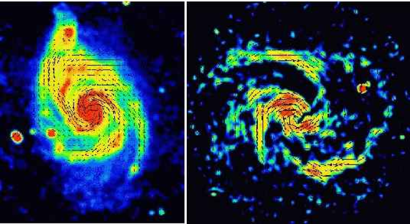
Figure 2.9: Left: M51 in $6\,{\rm cm}$, total intensity with magnetic field vectors. Right: NGC 6946 in $6\,{\rm cm}$, polarized intensity with magnetic field vectors. The physical extent of the images is approximately $28\times 34\,{\rm kpc}^{2}$ for M51 (distance $9.6\,{\rm Mpc}$) and $22\times 22\,{\rm kpc}^{2}$ for NGC 6946 (distance $7\,{\rm Mpc}$). (VLA and Effelsberg. Courtesy R. Beck.)

As we remarked earlier, RM observations are absolutely crucial to distinguish between coherent and incoherent fields. Coherence of RM on a large scale is indeed seen in a number of galaxies (for example, M31 [95], NGC 6946 [74], NGC 2997 [97]). The galaxy M31 seems to have a $20\,{\rm kpc}$ sized torus of emission, with the regular field nearly aligned with the spiral arms forming an emission ‘ring’, with an average pitch angle of about $-15^{\circ}$ [95, 98, 99]. Such a field can probably be produced only by a large scale dynamo.

The structure of the regular field is described in dynamo models by modes of different azimuthal and vertical symmetry; see Section 6.5.5. Again, Faraday rotation measure (RM) observations are crucial for this purpose [100]. The current data indicate a singly periodic azimuthal variation of RMs, suggesting a largely axisymmetric (ASS, $m=0$ symmetry) mean field structure in M31 [98] and IC 342 [101]. There is an indication of a bisymmetric spiral mode (BSS, $m=1$ symmetry) in M81 [102]. The field in M51 seems to be best described by a combination of ASS and BSS [103]. The magnetic arms in NGC 6946 may be the result of a superposition of ASS and quadrisymmetric ($m=2$) modes [73]. Indeed, in most galaxies the data cannot be described by only a single mode, but require a superposition of several modes which still cannot be resolved by the existing observations. It has also been noted [104] that in 4 out of 5 galaxies, the radial component of the spiral field could be such that the field points inward. This is remarkable in that the induction equation and the related nonlinearities do not distinguish between solutions $\bm{B}$ and $-\bm{B}$. An exception is the Hall effect where the direction matters [105], but this idea has not yet been applied to the field orientation in galaxies.

The vertical symmetry of the field is much more difficult to determine. The local field in our Galaxy is oriented mainly parallel to the plane (cf. [14, 77, 88]). This agrees well with the results from several other external edge-on galaxies [106], where the observed magnetic fields are generally aligned along the discs of the galaxies. Further, in our Galaxy the RMs of pulsars and extragalactic radio sources have the same sign above and below the galactic midplane, for galactic longitudes between $90^{\circ}$ and $270^{\circ}$, while toward the galactic center there is a claim that the RMs change sign cf. [107, 108]. This may point toward a vertically symmetric field in the Galaxy away from its central regions. Note that the determination of magnetic field structure in the Galaxy from Faraday rotation can be complicated by local perturbations. Taking into account such complications, and carrying out an analysis of the Faraday rotation measures of extragalactic sources using wavelet transforms, one finds evidence that the horizontal components of the regular magnetic field have even parity throughout the Galaxy, that is the horizontal components are similarly directed on both sides of the disc [109]. Note that a vertically symmetric field could arise from a quadrupolar meridional structure of the field, while vertically antisymmetric fields could arise from a dipolar structure. A vertically symmetric field also seems to be indicated from RM studies of the galaxy M31 [99].

The discovery of isolated non-thermal filaments throughout the inner few hundred parsecs of the galaxy [110, 111, 112] with orientations largely perpendicular to the galactic plane were interpreted as evidence for several milligauss level, space filling vertical fields in the central $200\,{\rm pc}$ of our galaxy [111]. However a recent $20\,{\rm cm}$ survey which has found numerous linear filaments finds them to have a wide range of orientations, which could complicate this simple picture [113, 114]. The observational situation needs to be clarified. If indeed the presence of a dipolar field in the galactic center regions is confirmed this would provide an important challenge for dynamo theory.

Although most edge-on galaxies have fields aligned along the disc, several galaxies (NGC 4631, NGC 4666 and M82) have also radio halos with a dominant vertical field component [73]. Magnetic spurs in these halos are connected to star forming regions in the disc. The field is probably dragged out by a strong, inhomogeneous galactic wind [115, 116].

Ordered magnetic fields with strengths similar to those in grand design spirals have also been detected in flocculent galaxies (M33 [BuB91], NGC 3521 and 5055 [117], NGC 4414 [118]), and even in irregular galaxies (NGC 4449 [119]). The mean degree of polarization is also similar between grand design and flocculent galaxies [117]. Also, a grand design spiral pattern is observed in all the above flocculent galaxies, implying that gaseous spiral arms are not an essential feature to obtain ordered fields.

There is little direct evidence on the nature of magnetic fields in elliptical galaxies, although magnetic fields may well be ubiquitous in the hot ionized gas seen in these galaxies [120]. This may be due to the paucity of relativistic electrons in these galaxies, which are needed to illuminate the magnetic fields by generating synchrotron emission. Faraday rotation of the polarized emission from background objects has been observed in a few cases. Particularly intriguing is the case of the gravitationally lensed twin quasar 0957+561, where the two images have a differential Faraday rotation of $\sim 100$ rad m^-2 [121]. One of the images passes through the central region of a possibly elliptical galaxy acting as the lens, and so this may indicate that the gas in this elliptical galaxy has ordered magnetic fields. It is important to search for more direct evidence for magnetic fields in elliptical galaxies.

2.5 Magnetic fields in clusters of galaxies

The most recent area of study of astrophysical magnetic fields is perhaps the magnetic fields of clusters of galaxies. Galaxy clusters are the largest bound systems in the universe, having masses of $\sim 10^{14}$–$10^{15}M_{\odot}$ and typical sizes of several $\,{\rm Mpc}$. Observations of clusters in X-rays reveal that they generally have an atmosphere of hot gas with temperatures $T\sim 10^{7}$ to $10^{8}$K, extending over $\,{\rm Mpc}$ scales. The baryonic mass of clusters is in fact dominated by this hot gas component. It has become clear in the last decade or so that magnetic fields are also ubiquitous in clusters. Succinct reviews of the observational data on cluster magnetic fields can be found in Ref. [122, 123]. Here we gather some important facts that are relevant in trying to understand the origin of these fields.

Evidence for magnetic fields in clusters again comes from mainly radio observations. Several clusters display relatively smooth low surface brightness radio halos, attributed to synchrotron emission from the cluster as a whole, rather than discrete radio sources. The first such halo to be discovered was that associated with the Coma cluster (called Coma C) [124]. Only recently have many more been found in systematic searches [125, 126, 127, 128]. These radio halos have typically sizes of $\sim 1$ Mpc, steep spectral indices, low surface brightness, low polarizations ($<5\%$ ), and are centered close to the center of the X-ray emission. Total magnetic fields in cluster radio halos, estimated using minimum energy arguments [129] range from $0.1$ to $1\,\mu{\rm G}$ [130], the value for Coma being $\sim 0.4\,\mu{\rm G}$ [131]. [The equipartition field will depend on the assumed proton to electron energy ratio; for a ratio of 100, like in the local ISM, the equipartition field will be larger by a factor $\sim 100^{2/7}\approx 3.7$ (R. Beck, private communication)].

Cluster magnetic fields can also be probed using Faraday rotation studies of both cluster radio galaxies and also background radio sources seen through the cluster. High resolution RM studies have been performed in several radio galaxies in both cooling flow clusters and non-cooling flow clusters (although the issue of the existence of cooling flows has become questionable). If one assumes a uniform field in the cluster, then minimum magnetic fields of $5$ to $10\,\mu{\rm G}$ are inferred in cooling flow clusters, whereas it could be a factor of 2 lower in non-cooling flow clusters [122]. However, the observed RM is patchy indicating magnetic field coherence scales of about $5$ to $10\,{\rm kpc}$ in these clusters. If we use such coherence lengths, then the estimated fields become larger. For example in the cooling flow cluster 3C295 the estimated magnetic field strength is $\sim 12\,\mu{\rm G}$ in the cluster core [132], whereas in the non-cooling flow cluster 3C129 the estimated field is about $6\,\mu{\rm G}$ [133]. In Hydra A, there is an intriguing trend for all the RMs to the north of the nucleus to be positive and to the south to be negative [134]. Naively this would indicate quite a large scale field ($100\,{\rm kpc}$) with strength $\sim 7\,\mu{\rm G}$ [134], but it is unclear which fraction is due to a cocoon surrounding the radio source (cf. Ref. [138]). The more tangled fields in the same cluster were inferred to have strengths of $\sim 30\,\mu{\rm G}$ and coherence lengths $\sim 4\,{\rm kpc}$ [134]. More recently, a novel technique to analyze Faraday rotation maps has been developed, assuming that the magnetic fields are statistically isotropic. This technique has been applied to several galaxy clusters [135, 136]. This analysis yields an estimate of $3\mu\,{\rm G}$ in Abell 2634, $6\mu\,{\rm G}$ in Abell 400 and $12\mu\,{\rm G}$ in Hydra A as conservative estimates of the field strengths, and field correlation lengths of $\sim 4.9\,{\rm kpc}$, $3.6\,{\rm kpc}$ and $0.9\,{\rm kpc}$, respectively, for these 3 clusters. (For Hydra A, a recent re-analysis of the data using an improved RM map and revised cluster parameters, has led to revised values of the central field of the cluster of $7\mu$G and correlation length of $3$ kpc, as well as a tentative determination of a Kolmogorov type magnetic power spectrum [137].)

Figure 2.10: Galaxy-corrected rotation measure plotted as a function of source impact parameter in kiloparsecs for the sample of 16 Abell clusters. The open points represent the cluster sources viewed through the thermal cluster gas while the closed points are the control sources at impact parameters beyond the cluster gas. Note the clear increase in the width of the RM distribution toward smaller impact parameter. Adapted from Clarke et al. [139].

There is always some doubt whether the RMs in cluster radio sources are produced due to Faraday rotation intrinsic to the radio source, rather than due to the intervening intracluster medium. While this is unlikely in most cases [122], perhaps more convincing evidence is the fact that studies of RMs of background radio sources seen through clusters, also indicate several $\,\mu{\rm G}$ cluster magnetic fields. A very interesting statistical study in this context is a recent VLA survey [139], where the RMs in and behind a sample of 16 Abell clusters were determined. The RMs were plotted as a function of distance from the cluster center and compared with a control sample of RMs from field sources; see Fig. 2.10. This study revealed a significant excess RM for sources within about $0.5\,{\rm Mpc}$ of the cluster center. Using a simple model, where the intracluster medium consists of cells of uniform size and field strength, but random field orientations, Clarke et al. [139] estimate cluster magnetic fields of $\sim 5\,(l/10\,{\rm kpc})^{-1/2}\,\mu{\rm G}$, where $l$ is the coherence length of the field.

Cluster magnetic fields can also be probed by comparing the inverse Compton X-ray emission and the synchrotron emission from the same region. Note that this ratio depends on the ratio of the background radiation energy density (which in many cases would be dominated by the Cosmic microwave background) to the magnetic field energy density. The main difficulty is in separating out the thermal X-ray emission. This separation can also be attempted using spatially resolved X-ray data. Indeed, an X-ray excess (compared to that expected from a thermal atmosphere) was seen at the location of a diffuse radio relic source in Abell 85 [140]. This was used in Ref. [140] to derive a magnetic field of $1.0\pm 0.1\,\,\mu{\rm G}$ for this source.

Overall it appears that there is considerable evidence that galaxy clusters are magnetized with fields ranging from a few $\,\mu{\rm G}$ to several tens of $\,\mu{\rm G}$ in some cluster centers, and with coherence scales of order $10\,{\rm kpc}$. These fields, if not maintained by some mechanism, will evolve as decaying MHD turbulence, and perhaps decay on the appropriate Alfvén time scale, which is $\sim 10^{8}$ yr, much less than the age of the cluster. We will have more to say on the possibility of dynamos in clusters in later sections toward the end of the review.

3 The equations of magnetohydrodynamics

In stars and galaxies, and indeed in many other astrophysical settings, the gas is partially or fully ionized and can carry electric currents that, in turn, produce magnetic fields. The associated Lorentz force exerted on the ionized gas (also called plasma) can in general no longer be neglected in the momentum equation for the gas. Magneto-hydrodynamics (MHD) is the study of the interaction of the magnetic field and the plasma treated as a fluid. In MHD we combine Maxwell’s equations of electrodynamics with the fluid equations, including also the Lorentz forces due to electromagnetic fields. We first discuss Maxwell’s equations that characterize the evolution of the magnetic field.

3.1 Maxwell’s equations

In gaussian cgs units, Maxwell’s equations can be written in the form

$${1\over c}{\partial\bm{B}\over\partial t}=-\bm{\nabla}\times\bm{E},\quad\bm{\nabla}\cdot\bm{B}=0,$$ (3.1)

$${1\over c}{\partial\bm{E}\over\partial t}=\bm{\nabla}\times\bm{B}-{4\pi\over c}\bm{J},\quad\bm{\nabla}\cdot\bm{E}=4\pi\rho_{\rm e},$$ (3.2)

where $\bm{B}$ is the magnetic flux density (usually referred to as simply the magnetic field), $\bm{E}$ is the electric field, $\bm{J}$ is the current density, $c$ is the speed of light, and $\rho_{\rm e}$ is the charge density.

Although in astrophysics one uses mostly cgs units, in much of the work on dynamos the MHD equations are written in ‘SI’ units, i.e. with magnetic permeability $\mu_{0}$ and without factors like $4\pi/c$. (Nevertheless, the magnetic field is still quoted often in gauss [G] and cgs units are used for density, lengths, etc.) Maxwell’s equations in SI units are then written as

$${\partial\bm{B}\over\partial t}=-\bm{\nabla}\times\bm{E},\quad\bm{\nabla}\cdot\bm{B}=0,$$ (3.3)

$${1\over c^{2}}{\partial\bm{E}\over\partial t}=\bm{\nabla}\times\bm{B}-\mu_{0}\bm{J},\quad\bm{\nabla}\cdot\bm{E}=\rho_{\rm e}/\epsilon_{0},$$ (3.4)

where $\epsilon_{0}=1/(\mu_{0}c^{2})$ is the permittivity of free space.

To ensure that $\bm{\nabla}\cdot\bm{B}=0$ is satisfied at all times it is often convenient to define $\bm{B}=\bm{\nabla}\times\bm{A}$ and to replace Eq. (3.3) by the ‘uncurled’ equation for the magnetic vector potential, $\bm{A}$,

$${\partial\bm{A}\over\partial t}=-\bm{E}-\bm{\nabla}\phi,$$ (3.5)

where $\phi$ is the scalar potential. Note that magnetic and electric fields are invariant under the gauge transformation

$$\bm{A}^{\prime}=\bm{A}+\bm{\nabla}\Lambda,$$ (3.6)

$$\phi^{\prime}=\phi-{\partial\Lambda\over\partial t}.$$ (3.7)

For numerical purposes it is often convenient to choose the gauge $\Lambda=\int\phi\,\mathrm{d}t$, which implies that $\phi^{\prime}=0$. Thus, instead of Eq. (3.5) one now solves the equation $\partial\bm{A}^{\prime}/\partial t=-\bm{E}$. There are a few other gauge choices that are numerically convenient (see, e.g., Section 8.1).

3.2 Resistive MHD and the induction equation

Using the standard Ohm’s law in a fixed frame of reference,

$$\bm{J}=\sigma\left(\bm{E}+\bm{U}\times\bm{B}\right),$$ (3.8)

where $\sigma$ is the electric conductivity, and introducing the magnetic diffusivity $\eta=(\mu_{0}\sigma)^{-1}$, or $\eta=c^{2}/(4\pi\sigma)$ in cgs units, we can eliminate $\bm{J}$ from Eq. (3.4), so we have

$$\left({1\over\eta}+{1\over c^{2}}{\partial\over\partial t}\right)\bm{E}=-\left({1\over\eta}\bm{U}-\bm{\nabla}\right)\times\bm{B}.$$ (3.9)

This formulation shows that the time derivative term (also called the Faraday displacement current) can be neglected if the relevant time scale over which the electric field varies, exceeds the Faraday time $\tau_{\rm Faraday}=\eta/c^{2}$. Below we shall discuss that for ordinary Spitzer resistivity, $\eta$ is proportional to $T^{-3/2}$ and varies between $10$ and $10^{10}\,{\rm cm}^{2}\,{\rm s}^{-1}$ for temperatures between $T=10^{8}$ and $T=10^{2}\,{\rm K}$. Thus, the displacement current can be neglected when the variation time scales are longer than $10^{-20}\,{\rm s}$ (for $T\approx 10^{8}\,{\rm K}$) and longer than $10^{-11}\,{\rm s}$ (for $T\approx 10^{2}\,{\rm K}$). For the applications discussed in this review, this condition is always met, even for neutron stars where the time scales of variation can be of the order of milliseconds, but the temperatures are very high as well. We can therefore safely neglect the displacement current and eliminate $\bm{E}$, so Eq. (3.4) can be replaced by Ampere’s law $\bm{J}=\bm{\nabla}\times\bm{B}/\mu_{0}$.

It is often convenient to consider $\bm{J}$ simply as a short hand for $\bm{\nabla}\times\bm{B}$. This can be accomplished by adopting units where $\mu_{0}=1$. We shall follow here this convection and shall therefore simply write

$$\bm{J}=\bm{\nabla}\times\bm{B}.$$ (3.10)

Occasionally we also state the full expressions for clarity.

Substituting Ohm’s law into the Faraday’s law of induction, and using Ampere’s law to eliminate $\bm{J}$, one can write a single evolution equation for $\bm{B}$, which is called the induction equation:

$${\partial\bm{B}\over\partial t}=\bm{\nabla}\times\left(\bm{U}\times\bm{B}-\eta\bm{J}\right).$$ (3.11)

We now describe a simple physical picture for the conductivity in a plasma. The force due to an electric field $\bm{E}$ accelerates electrons relative to the ions; but they cannot move freely due to friction with the ionic fluid, caused by electron–ion collisions. They acquire a ‘terminal’ relative velocity ${\bf V}$ with respect to the ions, obtained by balancing the Lorentz force with friction. This velocity can also be estimated as follows. Assume that electrons move freely for about an electron–ion collision time $\tau_{ei}$, after which their velocity becomes again randomized. Electrons of charge $e$ and mass $m_{e}$ in free motion during the time $\tau_{ei}$ acquire from the action of an electric field $\bm{E}$ an ordered speed ${\bf V}\sim\tau_{ei}e\bm{E}/m_{e}$. This corresponds to a current density $\bm{J}\sim en_{e}{\bf V}\sim(n_{e}e^{2}\tau_{ei}/m)\bm{E}$ and hence leads to $\sigma\sim n_{e}e^{2}\tau_{ei}/m_{e}$.

The electron–ion collision time scale (which determines $\sigma$) can also be estimated as follows. For a strong collision between an electron and an ion one needs an impact parameter $b$ which satisfies the condition $Ze^{2}/b>m_{e}v^{2}$. This gives a cross section for strong scattering of $\sigma_{t}\sim\pi b^{2}$. Since the Coulomb force is a long range force, the larger number of random weak scatterings add up to give an extra ‘Coulomb logarithm’ correction to make $\sigma_{t}\sim\pi(Ze^{2}/mv^{2})^{2}\ln\Lambda$, where $\ln\Lambda$ is in the range between 5 and 20. The corresponding mean free time between collisions is

$$\tau_{ei}\sim{1\over n_{i}\sigma_{t}v}\sim{(k_{\rm B}T)^{3/2}m_{e}^{1/2}\over\pi Ze^{4}n_{e}\ln\Lambda},$$ (3.12)

where we have used the fact that $m_{e}v^{2}\sim k_{\rm B}T$ and $Zn_{i}=n_{e}$. Hence we obtain the estimate

$$\sigma\sim{(k_{\rm B}T)^{3/2}\over m_{e}^{1/2}\pi Ze^{2}\ln\Lambda},$$ (3.13)

where most importantly the dependence on the electron density has canceled out. A more exact calculation can be found, for example, in Landau and Lifshitz [141] (Vol 10; Eq. 44.11) and gives an extra factor of $4(2/\pi)^{1/2}$ multiplying the above result. The above argument has ignored collisions between electrons themselves, and treated the plasma as a ‘lorentzian plasma’. The inclusion of the effect of electron–electron collisions further reduces the conductivity by a factor of about $0.582$ for $Z=1$ to $1$ for $Z\to\infty$; see the book by Spitzer [142], and Table 5.1 and Eqs. (5)–(37) therein, and leads to a diffusivity, in cgs units, of $\eta=c^{2}/(4\pi\sigma)$ given by

$$\eta=10^{4}\left({T\over 10^{6}\,{\rm K}}\right)^{-3/2}\left({\ln\Lambda\over 20}\right){\rm cm}^{2}{\rm s}^{-1}.$$ (3.14)

As noted above, the resistivity is independent of density, and is also inversely proportional to the temperature (larger temperatures implying larger mean free time between collisions, larger conductivity and hence smaller resistivity).

The corresponding expression for the kinematic viscosity $\nu$ is quite different. Simple kinetic theory arguments give $\nu\sim v_{\rm t}l_{i}$, where $l_{i}$ is the mean free path of the particles which dominate the momentum transport and $v_{\rm t}$ is their random velocity. For a fully ionized gas the ions dominate the momentum transport, and their mean free path $l_{i}\sim(n_{i}\sigma_{i})^{-1}$, with the cross-section $\sigma_{i}$, is determined again by the ion–ion ‘Coulomb’ interaction. From a reasoning very similar to the above for electron–ion collisions, we have $\sigma_{i}\sim\pi(Z^{2}e^{2}/k_{\rm B}T)^{2}\ln\Lambda$, where we have used $m_{i}v_{\rm t}^{2}\sim k_{\rm B}T$. Substituting for $v_{\rm t}$ and $l_{i}$, this then gives

$$\nu\sim{(k_{\rm B}T)^{5/2}\over n_{i}m_{i}^{1/2}\pi Z^{4}e^{4}\ln\Lambda}.$$ (3.15)

More accurate evaluation using the Landau collision integral gives a factor $0.4$ for a hydrogen plasma, instead of $1/\pi$ in the above expression (see the end of Section 43 in Vol. 10 of Landau and Lifshitz [141]). This gives numerically

$$\nu=6.5\times 10^{22}\left({T\over 10^{6}\,{\rm K}}\right)^{5/2}\left(n_{i}\over\,{\rm cm}^{-3}\right)^{-1}\left({\ln\Lambda\over 20}\right)^{-1}\,{\rm cm}^{2}\,{\rm s}^{-1},$$ (3.16)

so the magnetic Prandtl number is

$$P_{\rm m}\equiv{\nu\over\eta}=1.1\times 10^{-4}\left({T\over 10^{6}\,{\rm K}}\right)^{4}\left({\rho\over 0.1\,{\rm g}\,{\rm cm}^{-3}}\right)^{-1}\left({\ln\Lambda\over 20}\right)^{-2}.$$ (3.17)

Table 3.1: Summary of some important parameters in various astrophysical settings. The values given should be understood as rough indications only. In particular, the applicability of Eq. (3.17) is questionable in some cases and has therefore not been used for protostellar discs (see text). We have assumed $\ln\Lambda=20$ in computing $R_{\rm m}$ and $P_{\rm m}$. CZ means convection zone, CV discs and similar refer to cataclysmic variables and discs around other other compact objects such as black holes and neutron stars. AGNs are active galactic nuclei. Numbers in parenthesis indicate significant uncertainty due to other effects.

$T$ [K] $\rho\;[\,{\rm g}\,{\rm cm}^{-3}]$ $P_{\rm m}$ $u_{\rm rms}\;[\,{\rm cm}\,{\rm s}^{-1}]$ $L\;[\,{\rm cm}]$ $R_{\rm m}$ Solar CZ (upper part) $10^{4}$ $10^{-6}$ $10^{-7}$ $10^{6}$ $10^{8}$ $10^{6}$ Solar CZ (lower part) $10^{6}$ $10^{-1}$ $10^{-4}$ $10^{4}$ $10^{10}$ $10^{9}$ Protostellar discs $10^{3}$ $10^{-10}$ $10^{-8}$ $10^{5}$ $10^{12}$ $10$ CV discs and similar $10^{4}$ $10^{-7}$ $10^{-6}$ $10^{5}$ $10^{7}$ $10^{4}$ AGN discs $10^{7}$ $10^{-5}$ $10^{4}$ $10^{5}$ $10^{9}$ $10^{11}$ Galaxy $10^{4}$ $10^{-24}$ ($10^{11}$) $10^{6}$ $10^{20}$ ($10^{18}$) Galaxy clusters $10^{8}$ $10^{-26}$ ($10^{29}$) $10^{8}$ $10^{23}$ ($10^{29}$)

Thus, in the sun and other stars ($T\sim 10^{6}\,{\rm K}$, $\rho\sim 0.1\,{\rm g}\,{\rm cm}^{-3}$) the magnetic Prandtl number is much less than unity. Applied to the galaxy, using $T=10^{4}\,{\rm K}$ and $\rho=10^{-24}\,{\rm g}\,{\rm cm}^{-3}$, $\ln\Lambda\sim 10$, this formula gives $P_{\rm m}=4\times 10^{11}$. The reason $P_{\rm m}$ is so large in galaxies is mostly because of the very long mean free path caused by the low density [143]. For galaxy clusters, the temperature of the gas is even larger and the density smaller, making the medium much more viscous and having even larger $P_{\rm m}$.

In protostellar discs, on the other hand, the gas is mostly neutral with low temperatures. In this case, the electrical conductivity is given by $\sigma=n_{e}e^{2}\tau_{en}/m_{e}$, where $\tau_{en}$ is the rate of collisions between electrons and neutral particles. The associated resistivity is $\eta=234x_{e}^{-1}T^{1/2}\,{\rm cm}^{2}\,{\rm s}^{-1}$, where $x_{e}=n_{e}/n_{n}$ is the ionization fraction and $n_{n}$ is the number density of neutral particles [144]. The ionization fraction at the ionization–recombination equilibrium is approximately given by $x_{e}=(\zeta/\beta n_{n})^{1/2}$, where $\zeta$ is the ionization rate and $\beta=3\times 10^{-6}T^{-1/2}\,{\rm cm}^{3}\,{\rm s}^{-1}$ is the dissociative recombination rate [145, 146]. For a density of $\rho=10^{-10}\,{\rm g}\,{\rm cm}^{-3}$, and a mean molecular weight $2.33m_{p}$ [144], we have $n_{n}=2.6\times 10^{13}\,{\rm cm}^{-3}$. Adopting for $\zeta$ the cosmic ray ionizing rate $\zeta\sim 10^{-17}\,{\rm s}^{-1}$, which is not drastically attenuated by the dense gas in the disk, and a disc temperature $T=10^{3}\,{\rm K}$, we estimate $x_{e}\sim 2\times 10^{-12}$, and hence $\eta\sim 4\times 10^{15}\,{\rm cm}^{2}\,{\rm s}^{-1}$.

In Table LABEL:TAstrophysBodies we summarize typical values of temperature and density in different astrophysical settings and calculate the corresponding values of $P_{\rm m}$. Here we also give rough estimates of typical rms velocities, $u_{\rm rms}$, and eddy scales, $L$, which allow us to calculate the magnetic Reynolds number as

$$R_{\rm m}=u_{\rm rms}/(\eta k_{\rm f}),$$ (3.18)

where $k_{\rm f}=2\pi/L$. This number characterizes the relative importance of magnetic induction relative to magnetic diffusion. A similar number is the fluid Reynolds number, $\mbox{Re}=R_{\rm m}/P_{\rm m}$, which characterizes the relative importance of inertial forces to viscous forces. (We emphasize that in the above table, Reynolds numbers are defined based on the inverse wavenumber; our values may therefore be $2\pi$ times smaller that those by other authors. The present definition is a natural one in simulations where one forces power at a particular wavenumber around $k_{\rm f}$.)

3.3 Stretching, flux freezing and diffusion

The $\bm{U}\times\bm{B}$ term in Eq. (3.11) is usually referred to as the induction term. To clarify its role we rewrite its curl as

$$\bm{\nabla}\times\left(\bm{U}\times\bm{B}\right)=-\underbrace{\bm{U}\cdot\bm{\nabla}\bm{B}}_{\mbox{advection}}+\underbrace{\bm{B}\cdot\bm{\nabla}\bm{U}}_{\mbox{stretching}}-\underbrace{\bm{B}\bm{\nabla}\cdot\bm{U}}_{\mbox{compression}},$$ (3.19)

where we have used the fact that $\bm{\nabla}\cdot\bm{B}=0$. As a simple example, we consider the effect of a linear shear flow, $\bm{U}=(0,Sx,0)$ on the initial field $\bm{B}=(B_{0},0,0)$. The solution is $\bm{B}=(1,St,0)B_{0}$, i.e. the field component in the direction of the flow grows linearly in time.

The net induction term more generally implies that the magnetic flux through a surface moving with the fluid remains constant in the high-conductivity limit. Consider a surface $S$, bounded by a curve $C$, moving with the fluid, as shown in Fig. 3.1. Suppose we define the magnetic flux through this surface, $\Phi=\int_{S}\bm{B}\cdot\mathrm{d}\bm{S}$. Then after a time $\mathrm{d}t$ the change in flux is given by

$$\Delta\Phi=\int_{S^{\prime}}\bm{B}(t+\mathrm{d}t)\cdot\mathrm{d}\bm{S}-\int_{S}\bm{B}(t)\cdot\mathrm{d}\bm{S}.$$ (3.20)

Applying $\int\bm{\nabla}\cdot\bm{B}\,\mathrm{d}V=0$ at time $t+\mathrm{d}t$, to the ‘tube’-like volume swept up by the moving surface $S$, shown in Fig. 3.1, we also have

$$\int_{S^{\prime}}\bm{B}(t+\mathrm{d}t)\cdot\mathrm{d}\bm{S}=\int_{S}\bm{B}(t+\mathrm{d}t)\cdot\mathrm{d}\bm{S}-\oint_{C}\bm{B}(t+\mathrm{d}t)\cdot(\mathrm{d}\bm{l}\times\bm{U}\mathrm{d}t),$$ (3.21)

where $C$ is the curve bounding the surface $S$, and $\mathrm{d}\bm{l}$ is the line element along $C$. (In the last term, to linear order in $\mathrm{d}t$, it does not matter whether we take the integral over the curve $C$ or $C^{\prime}$.) Using the above condition in Eq. (3.20), we obtain

$$\Delta\Phi=\int_{S}[\bm{B}(t+\mathrm{d}t)-\bm{B}(t)]\cdot\mathrm{d}\bm{S}-\oint_{C}\bm{B}(t+\mathrm{d}t)\cdot(\mathrm{d}\bm{l}\times\bm{U})\mathrm{d}t.$$ (3.22)

Taking the limit of $\mathrm{d}t\to 0$, and noting that $\bm{B}\cdot(\mathrm{d}\bm{l}\times\bm{U})=(\bm{U}\times\bm{B})\cdot\mathrm{d}\bm{l}$, we have

$${d\Phi\over\mathrm{d}t}=\int_{S}{\partial\bm{B}\over\partial t}\cdot\mathrm{d}\bm{S}-\oint_{C}(\bm{U}\times\bm{B})\cdot\mathrm{d}\bm{l}=-\int_{S}(\nabla\times\eta\bm{J})\cdot\mathrm{d}\bm{S}.$$ (3.23)

In the second equality we have used $\oint_{C}(\bm{U}\times\bm{B})\cdot\mathrm{d}\bm{l}=\int_{S}\bm{\nabla}\times(\bm{U}\times\bm{B})\cdot\mathrm{d}\bm{S}$ together with the induction equation (3.11). One can see that, when $\eta\to 0$, $\mathrm{d}\Phi/\mathrm{d}t\to 0$ and so $\Phi$ is constant.

Figure 3.1: The surface $S$ enclosed by the curve $C$ is carried by fluid motion to the surface $S^{\prime}$ after a time $\mathrm{d}t$. The flux through this surface $\Phi$ is frozen into the fluid for a perfectly conducting fluid.

Now suppose we consider a small segment of a thin flux tube of length $l$ and cross-section $A$, in a highly conducting fluid. Then, as the fluid moves about, conservation of flux implies $BA$ is constant, and conservation of mass implies $\rho Al$ is constant, where $\rho$ is the local density. So $B\propto\rho l$. For a nearly incompressible fluid, or a flow with small changes in $\rho$, one will obtain $B\propto l$. Any shearing motion which increases $l$ will also amplify $B$; an increase in $l$ leading to a decrease in $A$ (because of incompressibility) and hence an increase in $B$ (due to flux freezing). This effect, also obtained in our discussion of stretching above, will play a crucial role in all scenarios involving dynamo generation of magnetic fields.

The concept of flux freezing can also be derived from the elegant Cauchy solution of the induction equation with zero diffusion. This solution is of use in several contexts and so we describe it briefly below. In the case $\eta=0$, the $\bm{\nabla}\times(\bm{U}\times\bm{B})$ term in Eq. (3.11) can be expanded to give

$${\mathrm{D}\bm{B}\over\mathrm{D}t}=\bm{B}\cdot\bm{\nabla}\bm{U}-\bm{B}(\bm{\nabla}\cdot\bm{U}),$$ (3.24)

where $\mathrm{D}/\mathrm{D}t=\partial/\partial t+\bm{U}\cdot\bm{\nabla}$ is the lagrangian derivative. If we eliminate the $\bm{\nabla}\cdot\bm{U}$ term using the continuity equation for the fluid,

$${\partial\rho\over\partial t}=-\bm{\nabla}\cdot(\rho\bm{U}),$$ (3.25)

where $\rho$ is the fluid density, then we can write

$${\mathrm{D}\over\mathrm{D}t}\left({\bm{B}\over\rho}\right)={\bm{B}\over\rho}\cdot\bm{\nabla}\bm{U}.$$ (3.26)

Suppose we describe the evolution of a fluid element by giving its trajectory as $\bm{x}(\bm{x}_{0},t)$, where $\bm{x}_{0}$ is its location at an initial time $t_{0}$. Consider further the evolution of two infinitesimally separated fluid elements, $A$ and $B$, which, at an initial time $t=t_{0}$, are located at $\bm{x}_{0}$ and $\bm{x}_{0}+\delta\bm{x}_{0}$, respectively. The subsequent location of these fluid elements will be, say, $\bm{x}_{A}=\bm{x}(\bm{x}_{0},t)$ and $\bm{x}_{B}=\bm{x}(\bm{x}_{0}+\delta\bm{x}_{0},t)$ and their separation is $\bm{x}_{B}-\bm{x}_{A}=\delta\bm{x}(\bm{x}_{0},t)$. Since the velocity of the fluid particles will be $\bm{U}(\bm{x}_{A})$ and $\bm{U}(\bm{x}_{A})+\delta\bm{x}\cdot\bm{\nabla}\bm{U}$, after a time $\delta t$, the separation of the two fluid particles will change by $\delta t\,\delta\bm{x}\cdot\bm{\nabla}\bm{U}$. The separation vector therefore evolves as

$${\mathrm{D}\delta\bm{x}\over\mathrm{D}t}=\delta\bm{x}\cdot\bm{\nabla}\bm{U},$$ (3.27)

which is an evolution equation identical to that satisfied by $\bm{B}/\rho$. So, if initially, at time $t=t_{0}$, the fluid particles were on a given magnetic field line with $(\bm{B}/\rho)(\bm{x}_{0},t_{0})=c_{0}\delta\bm{x}(t_{0})=c_{0}\delta\bm{x}_{0}$, where $c_{0}$ is a constant, then for all times we will have $\bm{B}/\rho=c_{0}\delta\bm{x}$. In other words, ‘if two infinitesimally close fluid particles are on the same line of force at any time, then they will always be on the same line of force, and the value of $\bm{B}/\rho$ will be proportional to the distance between the particles’ (Section 65 in Ref. [147]). Further, since $\delta x_{i}(\bm{x}_{0},t)={\sf G}_{ij}\delta x_{0j}$, where ${\sf G}_{ij}=\partial x_{i}/\partial x_{0j}$, we can also write

$$B_{i}(\bm{x},t)=\rho c_{0}\delta x_{i}={{\sf G}_{ij}(\bm{x}_{0},t)\over\det{\bf G}{}}\,B_{0j}(\bm{x}_{0}),$$ (3.28)

where we have used the fact that $\rho(\bm{x},t)/\rho(\bm{x}_{0},t_{0})=(\det{\bf G}{})^{-1}$. We will use this Cauchy solution in Appendix B.1.

3.4 Magnetic helicity

Magnetic helicity plays an important role in dynamo theory. We therefore give here a brief account of its properties. Magnetic helicity is the volume integral

$$H=\int_{V}\bm{A}\cdot\bm{B}\;\mathrm{d}V$$ (3.29)

over a closed or periodic volume $V$. By a closed volume we mean one in which the magnetic field lines are fully contained, so the field has no component normal to the boundary, i.e. $\bm{B}\cdot\bm{n}=0$. The volume $V$ could also be an unbounded volume with the fields falling off sufficiently rapidly at spatial infinity. In these particular cases, $H$ is invariant under the gauge transformation (3.6), because

$$H^{\prime}=\int_{V}\bm{A}^{\prime}\cdot\bm{B}^{\prime}\;\mathrm{d}V=H+\int_{V}\bm{\nabla}\Lambda\cdot\bm{B}\;\mathrm{d}V=H+\oint_{\partial V}\Lambda\bm{B}\cdot\hat{\mbox{\boldmath$n$}}{}\mathrm{d}S=H,$$ (3.30)

where $\hat{\mbox{\boldmath$n$}}{}$ is the normal pointing out of the closed surface $\partial V$. Here we have made use of $\bm{\nabla}\cdot\bm{B}=0$.

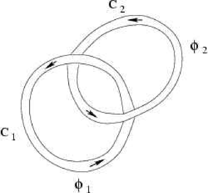
Figure 3.2: Two flux tubes with fluxes $\Phi_{1}$ and $\Phi_{2}$ are linked in such a way that they have a helicity $H=+2\Phi_{1}\Phi_{2}$. Interchanging the direction of the field in one of the two rings changes the sign of $H$.

Magnetic helicity has a simple topological interpretation in terms of the linkage and twist of isolated (non-overlapping) flux tubes. For example consider the magnetic helicity for an interlocked, but untwisted, pair of thin flux tubes as shown in Fig. 3.2, with $\Phi_{1}$ and $\Phi_{2}$ being the fluxes in the tubes around $C_{1}$ and $C_{2}$ respectively. For this configuration of flux tubes, $\bm{B}\,\mathrm{d}^{3}x$ can be replaced by $\Phi_{1}\mathrm{d}\bm{l}$ on $C_{1}$ and $\Phi_{2}\mathrm{d}\bm{l}$ on $C_{2}$. The net helicity is then given by the sum

$$H=\Phi_{1}\oint_{C_{1}}\bm{A}\cdot\mathrm{d}\bm{l}+\Phi_{2}\oint_{C_{2}}\bm{A}\cdot\mathrm{d}\bm{l},=2\Phi_{1}\Phi_{2}$$ (3.31)

where we have used Stokes theorem to transform

$$\oint_{C_{1}}\bm{A}\cdot\mathrm{d}\bm{l}=\!\!\int_{S(C_{1})}\!\!\bm{B}\cdot\mathrm{d}\bm{S}\equiv\Phi_{2},\quad\quad\oint_{C_{2}}\bm{A}\cdot\mathrm{d}\bm{l}=\!\!\int_{S(C_{2})}\!\!\bm{B}\cdot\mathrm{d}\bm{S}\equiv\Phi_{1}.$$ (3.32)

For a general pair of non-overlapping thin flux tubes, the helicity is given by $H=\pm 2\Phi_{1}\Phi_{2}$; the sign of $H$ depending on the relative orientation of the two tubes [148].

The evolution equation for $H$ can be derived from Faraday’s law and its uncurled version for $\bm{A}$, Eq. (3.5), so we have

$${\partial\over\partial t}(\bm{A}\cdot\bm{B}) = (-\bm{E}+\bm{\nabla}\phi)\cdot\bm{B}+\bm{A}\cdot(-\bm{\nabla}\times\bm{E})$$ (3.33)

$$= -2\bm{E}\cdot\bm{B}+\bm{\nabla}\cdot(\phi\bm{B}+\bm{A}\times\bm{E}).$$

Integrating this over the volume $V$, the magnetic helicity satisfies the evolution equation

$${\mathrm{d}H\over\mathrm{d}t}=-2\int_{V}\bm{E}\cdot\bm{B}\mathrm{d}V+\oint_{\partial V}(\bm{A}\times\bm{E}+\phi\bm{B})\cdot\hat{\mbox{\boldmath$n$}}{}\mathrm{d}S=-2\eta C,$$ (3.34)

where $C=\int_{V}\bm{J}\cdot\bm{B}\;\mathrm{d}V$ is the current helicity. Here we have used Ohm’s law, $\bm{E}=-\bm{U}\times\bm{B}+\eta\bm{J}$, in the volume integral and we have assumed that the surface integral vanishes for closed domains. If the $\mu_{0}$ factor were included, this equation would read $\mathrm{d}H/\mathrm{d}t=-2\eta\mu_{0}C$.

In the non-resistive case, $\eta=0$, the magnetic helicity is conserved, i.e. $\mathrm{d}H/\mathrm{d}t=0$. However, this does not guarantee conservation of $H$ in the limit $\eta\rightarrow 0$, because the current helicity, $\int\bm{J}\cdot\bm{B}\,\mathrm{d}V$, may in principle still become large. For example, the Ohmic dissipation rate of magnetic energy $Q_{\rm Joule}\equiv\int\eta{\bf J}^{2}\mathrm{d}V$ can be finite and balance magnetic energy input by motions, even when $\eta\rightarrow 0$. This is because small enough scales develop in the field (current sheets) where the current density increases with decreasing $\eta$ as $\propto\eta^{-1/2}$ as $\eta\rightarrow 0$, whilst the rms magnetic field strength, $B_{\rm rms}$, remains essentially independent of $\eta$. Even in this case, however, the rate of magnetic helicity dissipation decreases with $\eta$, with an upper bound to the dissipation rate $\propto\eta^{+1/2}\rightarrow 0$, as $\eta\rightarrow 0$. Thus, under many astrophysical conditions where $R_{\rm m}$ is large ($\eta$ small), the magnetic helicity $H$, is almost independent of time, even when the magnetic energy is dissipated at finite rates. This robust conservation of magnetic helicity is an important constraint on the nonlinear evolution of dynamos and will play a crucial role below in determining how large scale turbulent dynamos saturate. Indeed, it is also at the heart of Taylor relaxation in laboratory plasmas, where an initially unstable plasma relaxes to a stable ‘force-free’ state, dissipating energy, while nearly conserving magnetic helicity [149].

We also note the very important fact that the fluid velocity completely drops out from the helicity evolution equation (3.34), since $(\bm{U}\times\bm{B})\cdot\bm{B}=0$. Therefore, any change in the nature of the fluid velocity, for example due to turbulence (turbulent diffusion), the Hall effect, or ambipolar drift (see below), does not affect magnetic helicity conservation. We will discuss in more detail the concept of turbulent diffusion in a later section, and its role in dissipating the mean magnetic field. However, such turbulent magnetic diffusion does not dissipate the net magnetic helicity. This property is crucial for understanding why, in spite of the destructive properties of turbulence, large scale spatio-temporal coherence can emerge if there is helicity in the system.

For open volumes, or volumes with boundaries through which $\bm{B}\cdot\hat{\mbox{\boldmath$n$}}{}\neq 0$, the magnetic helicity $H$, as defined by Eq. (3.29), is no longer gauge-invariant. One can define a gauge-invariant relative magnetic helicity [150, 151, 152]

$$H_{\rm rel}=\int_{V}(\bm{A}+\bm{A}^{\rm ref})\cdot(\bm{B}-\bm{B}^{\rm ref})\;\mathrm{d}V,$$ (3.35)

where $\bm{B}^{\rm ref}=\bm{\nabla}\times\bm{A}^{\rm ref}$ is a reference magnetic field that is taken to be the potential field solution (where $\bm{B}^{\rm ref}=\bm{\nabla}\varphi$ is the gradient of a potential, so there is no current), with the boundary condition

$$\hat{\mbox{\boldmath$n$}}{}\cdot\bm{B}^{\rm ref}=\hat{\mbox{\boldmath$n$}}{}\cdot\bm{B},$$ (3.36)

i.e. the two fields have the same normal components. The quantity $H_{\rm rel}$ is gauge-invariant, because in Eq. (3.30) the term $\hat{\mbox{\boldmath$n$}}{}\cdot\bm{B}$ is replaced by $\hat{\mbox{\boldmath$n$}}{}\cdot(\bm{B}-\bm{B}^{\rm ref})$, which vanishes on the boundaries.

The evolution equation of the relative magnetic helicity is simplified by adopting a specific gauge for $\bm{A}^{\rm ref}$, with

$$\bm{\nabla}\cdot\bm{A}^{\rm ref}=0,\quad\bm{A}^{\rm ref}\cdot\hat{\mbox{\boldmath$n$}}{}|_{\partial V}=0.$$ (3.37)

We point out, however, that this restriction can in principle be relaxed. When the gauge (3.37) is used for the reference field, the relative magnetic helicity satisfies the evolution equation

$${\mathrm{d}H_{\rm rel}\over\mathrm{d}t}=-2\eta C-2\oint_{\partial V}(\bm{E}\times\bm{A}^{\rm ref})\cdot\mathrm{d}\bm{S},$$ (3.38)

where $\mathrm{d}\bm{S}=\hat{\mbox{\boldmath$n$}}{}\,\mathrm{d}S$ is the surface element. The surface integral covers the full closed surface around the volume $V$. In the case of the sun the magnetic helicity fluxes from the northern and southern hemispheres are expected to be about equally big and of opposite sign, so they would cancel approximately to zero. One is therefore usually interested in the magnetic helicity flux out of the northern or southern hemispheres, but this means that it is necessary to include the contribution of the equator to the surface integral in Eq. (3.38). This contribution can easily be calculated for data from numerical simulations, but in the case of the sun the contribution from the equatorial surface is not observed.

We should point out that it is also possible to define magnetic helicity as linkages of flux analogous to the Gauss linking formula for linkages of curves. We have recently used this approach to formulate the concept of a gauge invariant magnetic helicity density in the case of random fields, whose correlation length is much smaller than the system size [154].

We have emphasized earlier in this section that no net magnetic helicity can be produced by any kind of velocity. However, this is not true of the magnetic helicity flux which is affected by the velocity via the electric field. This can be important if there is differential rotation or shear which can lead to a separation of magnetic helicity in space. A somewhat related mechanism is the alpha effect (Section 6) which can lead to a separation of magnetic helicity in wavenumber space. Both processes are important in the sun or the galaxy.

3.5 The momentum equation

Finally we come to the momentum equation, which is just the ordinary Navier-Stokes equation in fluid dynamics supplemented by the Lorentz force, $\bm{J}\times\bm{B}$, i.e.

$$\rho{\mathrm{D}\bm{U}\over\mathrm{D}t}=-\bm{\nabla}p+\bm{J}\times\bm{B}+\bm{f}+\bm{F}_{\rm visc},$$ (3.39)

where $\bm{U}$ is the ordinary bulk velocity of the gas, $\rho$ is the density, $p$ is the pressure, $\bm{F}_{\rm visc}$ is the viscous force, and $\bm{f}$ subsumes all other body forces acting on the gas, including gravity and, in a rotating system also the Coriolis and centrifugal forces. (We use an upper case $\bm{U}$, because later on we shall use a lower case $\bm{u}$ for the fluctuating component of the velocity.) Equation (3.39) has to be supplemented by the continuity equation,

$${\partial\rho\over\partial t}=-\bm{\nabla}\cdot(\rho\bm{U}),$$ (3.40)

an equation of state, $p=p(\rho,e)$, an energy equation for the internal energy $e$, and an evolution equation for the magnetic field.

An important quantity is the adiabatic sound speed, $c_{\rm s}$, defined as $c_{\rm s}^{2}=(\partial p/\partial\rho)_{s}$, evaluated at constant entropy $s$. For a perfect gas with constant ratio $\gamma$ of specific heats ($\gamma=5/3$ for a monatomic gas) we have $c_{\rm s}^{2}=\gamma p/\rho$. When the flow speed is much smaller than the sound speed, i.e. when the average Mach number $\mbox{Ma}=\langle\bm{U}^{2}/c_{\rm s}^{2}\rangle^{1/2}$ is much smaller than unity and if, in addition, the density is approximately uniform, i.e. $\rho\approx\rho_{0}={\rm const}$, the assumption of incompressibility can be made. In that case, Eq. (3.25) can be replaced by $\bm{\nabla}\cdot\bm{U}=0$, and the momentum equation then simplifies to

$${\mathrm{D}\bm{U}\over\mathrm{D}t}=-{1\over\rho_{0}}\bm{\nabla}p+{\bm{J}\times\bm{B}\over\rho_{0}}+\bm{f}+\nu\nabla^{2}\bm{U},$$ (3.41)

where $\nu$ is the kinematic viscosity and $\bm{f}$ is now an external body force per unit mass. The ratio $P_{\rm m}=\nu/\eta$ is the magnetic Prandtl number; see Eq. (3.17).

The assumption of incompressibility is a great simplification that is useful for many analytic considerations, but for numerical solutions this restriction is often not necessary. As long as the Mach number is small, say below 0.3, the weakly compressible case is believed to be equivalent to the incompressible case [155].

3.6 Kinetic helicity evolution

We introduce the vorticity $\bm{W}=\bm{\nabla}\times\bm{U}$, and define the kinetic helicity as $F=\int\bm{W}\cdot\bm{U}\;\mathrm{d}V$. Using Eq. (3.41), and ignoring the magnetic field, $F$ obeys the evolution equation

$${\mathrm{d}F\over\mathrm{d}t}=2\int\bm{W}\cdot\bm{f}\;\mathrm{d}V-2\nu\int\bm{W}\cdot\bm{Q}\;\mathrm{d}V,$$ (3.42)

where $\bm{Q}=\bm{\nabla}\times\bm{W}$ is the curl of the vorticity. Note that in the absence of forcing, $\bm{f}=0$, and without viscosity, $\nu=0$, the kinetic helicity is conserved, i.e.

$${\mathrm{d}F\over\mathrm{d}t}=0\quad\mbox{(if $\nu=0$ and $\bm{f}=0$)}.$$ (3.43)

On the other hand, in the limit $\nu\to 0$ (which is different from the case $\nu=0$) the rate of kinetic helicity production will not converge to zero with decreasing values of $\nu$. This is a major difference to magnetic helicity conservation, where the rate of helicity production converges to zero at low resistivity. Ignoring compressibility effects, i.e. $\rho=\mbox{const}$, this follows by assuming that both kinetic energy, ${\textstyle{1\over 2}}\int\bm{U}^{2}\mathrm{d}V$, and the rate of kinetic energy dissipation, $\epsilon=\nu\int\bm{W}^{2}\mathrm{d}V$, are independent of $\nu$. Therefore, both the magnitude of the vorticity, $|\bm{W}|$, and the typical wavenumber $k_{\nu}$ associated with $|\bm{W}|\approx k_{\nu}|\bm{U}|$ scale like $k_{\nu}\sim\nu^{-1/2}$. Thus, $|\bm{Q}|\sim k_{\nu}|\bm{W}|\sim\nu^{-1}$, so $\nu|\bm{W}\cdot\bm{Q}|\sim\nu^{-1/2}$, and hence

$$\left|{\mathrm{d}F\over\mathrm{d}t}\right|\sim\nu^{-1/2}\to\infty\quad\mbox{(for $\nu\to 0$)}.$$ (3.44)

For comparison (as we pointed out earlier), in the magnetic case, the current density also diverges like $|\bm{J}|\sim\eta^{-1/2}$, but the rate of magnetic helicity production is only proportional to $\bm{J}\cdot\bm{B}$, and $\eta\bm{J}\cdot\bm{B}\sim\eta^{+1/2}\to 0$, so

$$\left|{\mathrm{d}H\over\mathrm{d}t}\right|\sim\eta^{+1/2}\to 0\quad\mbox{(for $\eta\to 0$)}.$$ (3.45)

It is worth emphasizing again that it is for this reason that the magnetic helicity is such an important quantity in magnetohydrodynamics.

3.7 Energy and helicity spectra

Magnetic energy and helicity spectra are usually calculated as

$$M_{k}=\frac{1}{2}\int_{\mbox{$k$-shell}}\bm{B}_{\bm{k}}^{*}\cdot\bm{B}_{\bm{k}}\,k^{2}\,\mathrm{d}\Omega_{k},$$ (3.46)

$$H_{k}=\frac{1}{2}\int_{\mbox{$k$-shell}}(\bm{A}_{\bm{k}}^{*}\cdot\bm{B}_{\bm{k}}+\bm{A}_{\bm{k}}\cdot\bm{B}_{\bm{k}}^{*})\,k^{2}\,\mathrm{d}\Omega_{\bm{k}},$$ (3.47)

where $\mathrm{d}\Omega_{\bm{k}}$ is the solid angle element in Fourier space, $\bm{B}_{\bm{k}}=\mathrm{i}\bm{k}\times\bm{A}_{\bm{k}}$ is the Fourier transform of the magnetic field, and $\bm{A}_{\bm{k}}$ is the Fourier transform of the vectors potential. These spectra are normalized such that

$$\int_{0}^{\infty}H_{k}\,\mathrm{d}k=\langle\bm{A}\cdot\bm{B}\rangle V\equiv H,$$ (3.48)

$$\int_{0}^{\infty}M_{k}\,\mathrm{d}k=\langle{\textstyle{1\over 2}}\bm{B}^{2}\rangle V\equiv M,$$ (3.49)

where $H$ and $M$ are magnetic helicity and magnetic energy, respectively, and angular brackets denote volume averages.

There is a conceptual advantage [4] in working with the real space Fourier filtered magnetic vector potential and magnetic field, $\bm{A}_{k}$ and $\bm{B}_{k}$, where $\bm{B}_{k}=\bm{\nabla}\times\bm{A}_{k}$, and the subscript $k$ (which is now a scalar!) indicates Fourier filtering to keep only those wavevectors $\bm{k}$ that lie in the shell

$$k-\delta k/2\leq|\bm{k}|<k+\delta k/2\quad(\mbox{$k$-shell}).$$ (3.50)

Magnetic energy and helicity spectra can then be written as

$$M_{k}={\textstyle{1\over 2}}\langle\bm{B}_{k}^{2}\rangle V/\delta k,$$ (3.51)

$$H_{k}=\langle\bm{A}_{k}\cdot\bm{B}_{k}\rangle V/\delta k,$$ (3.52)

where angular brackets denote averages over all space. We recall that, for a periodic domain, $H$ is gauge invariant. Since its spectrum can be written as an integral over all space, see Eq. (3.52), $H_{k}$ is – like $H$ – also gauge invariant.

It is convenient to decompose the Fourier transformed magnetic vector potential, $\bm{A}_{\bm{k}}$, into a longitudinal component, $\bm{h}^{\parallel}$, and eigenfunctions $\bm{h}^{\pm}$ of the curl operator. Especially in the context of spherical domains these eigenfunctions are also called Chandrasekhar–Kendall functions [156], while in cartesian domains they are usually referred to as Beltrami waves. This decomposition has been used in studies of turbulence [157], in magnetohydrodynamics [158], and in dynamo theory [159]. Using this decomposition we can write the Fourier transformed magnetic vector potential as

$$\bm{A}_{\bm{k}}=a_{\bm{k}}^{+}\bm{h}_{\bm{k}}^{+}+a_{\bm{k}}^{-}\bm{h}_{\bm{k}}^{-}+a_{\bm{k}}^{\parallel}\bm{h}_{\bm{k}}^{\parallel},$$ (3.53)

with

$$\mathrm{i}\bm{k}\times\bm{h}_{\bm{k}}^{\pm}=\pm k\bm{h}_{\bm{k}}^{\pm},\quad\quad k=|\bm{k}|,$$ (3.54)

and

$$\langle{\bm{h}_{\bm{k}}^{+}}^{*}\cdot\bm{h}_{\bm{k}}^{+}\rangle=\langle{\bm{h}_{\bm{k}}^{-}}^{*}\cdot\bm{h}_{\bm{k}}^{-}\rangle=\langle{\bm{h}_{\bm{k}}^{\parallel}}^{*}\cdot{\bm{h}_{\bm{k}}^{\parallel}}\rangle=1,$$ (3.55)

where asterisks denote the complex conjugate, and angular brackets denote, as usual, volume averages. The longitudinal part $a_{\bm{k}}^{\parallel}\bm{h}_{\bm{k}}^{\parallel}$ is parallel to $\bm{k}$ and vanishes after taking the curl to calculate the magnetic field. In the Coulomb gauge, $\nabla\cdot\bm{A}=0$, the longitudinal component vanishes altogether.

The (complex) coefficients $a_{\bm{k}}^{\pm}(t)$ depend on $\bm{k}$ and $t$, while the eigenfunctions $\bm{h}_{\bm{k}}^{\pm}$, which form an orthonormal set, depend only on $\bm{k}$ and are given by

$$\bm{h}_{\bm{k}}^{\pm}=\frac{1}{\sqrt{2}}{\bm{k}\times(\bm{k}\times\bm{e})\mp\mathrm{i}k(\bm{k}\times\bm{e})\over k^{2}\sqrt{1-(\bm{k}\cdot\bm{e})^{2}/k^{2}}},$$ (3.56)

where $\bm{e}$ is an arbitrary unit vector that is not parallel to $\bm{k}$. With these preparations we can write the magnetic helicity and energy spectra in the form

$$H_{k}=k(|a^{+}|^{2}-|a^{-}|^{2})V,$$ (3.57)

$$M_{k}={\textstyle{1\over 2}}k^{2}(|a^{+}|^{2}+|a^{-}|^{2})V,$$ (3.58)

where $V$ is the volume of integration. (Here again the factor $\mu_{0}^{-1}$ is ignored in the definition of the magnetic energy.) From Eqs. (3.57) and (3.58) one sees immediately that [148, 159]

$${\textstyle{1\over 2}}k|H_{k}|\leq M_{k},$$ (3.59)

which is also known as the realizability condition. A fully helical field has therefore $M_{k}=\pm{\textstyle{1\over 2}}kH_{k}$.

For further reference we now define power spectra of those components of the field that are either right or left handed, i.e.

$$H_{k}^{\pm}=\pm k|a_{\pm}|^{2}V,\quad M_{k}^{\pm}={\textstyle{1\over 2}}k^{2}|a_{\pm}|^{2}V.$$ (3.60)

Thus, we have $H_{k}=H_{k}^{+}+H_{k}^{-}$ and $M_{k}=M_{k}^{+}+M_{k}^{-}$. Note that $H_{k}^{\pm}$ and $M_{k}^{\pm}$ can be calculated without explicit decomposition into right and left handed field components using

$$H_{k}^{\pm}={\textstyle{1\over 2}}(H_{k}\pm 2k^{-1}M_{k}),\quad M_{k}^{\pm}={\textstyle{1\over 2}}(M_{k}\pm{\textstyle{1\over 2}}kH_{k}).$$ (3.61)

This method is significantly simpler than invoking explicitly the decomposition in terms of $a_{\bm{k}}^{\pm}\bm{h}_{\bm{k}}^{\pm}$.

In Section 8.3 plots of $M_{k}^{\pm}$ will be shown and discussed in connection with turbulence simulations. Here the turbulence is driven with a helical forcing function proportional to $\bm{h}_{\bm{k}}^{+}$; see Eq. (3.56).

3.8 Departures from the one–fluid approximation

In many astrophysical settings the typical length scales are so large that the usual estimates for the turbulent diffusion of magnetic fields, by far exceed the ordinary Spitzer resistivity. Nevertheless, the net magnetic helicity evolution, as we discussed above, is sensitive to the microscopic resistivity and independent of any turbulent contributions. It is therefore important to discuss in detail the foundations of Spitzer resistivity and to consider more general cases such as the two–fluid and even three–fluid models. In some cases these generalizations lead to important effects of their own, for example the battery effect.

3.8.1 Two–fluid approximation

The simplest generalization of the one–fluid model is to consider the electrons and ions as separate fluids which are interacting with each other through collisions. This two–fluid model is also essential for deriving the general form of Ohm’s law and for describing battery effects, that generate fields ab-initio from zero initial field. We therefore briefly consider it below.

For simplicity assume that the ions have one charge, and in fact they are just protons. That is the plasma is purely ionized hydrogen. It is straightforward to generalize these considerations to several species of ions. The corresponding set of fluid equations, incorporating the non-ideal properties of the fluids and the anisotropy induced by the presence of a magnetic field, is worked out and summarized by Braginsky [160]. For our purpose it suffices to follow the simple treatment of Spitzer [142], where we take the stress tensor to be just isotropic pressure, leaving out non-ideal terms, and also adopt a simple form for the collision term between electrons and protons. The equations of motion for the electron and proton fluids may then be written as

$${D_{e}\bm{u}_{e}\over Dt}=-{\bm{\nabla}p_{e}\over n_{e}m_{e}}-{e\over m_{e}}\left(\bm{E}+\bm{u}_{e}\times\bm{B}\right)-\bm{\nabla}\phi_{g}-{(\bm{u}_{e}-\bm{u}_{p})\over\tau_{ei}},$$ (3.62)

$${D_{i}\bm{u}_{i}\over Dt}=-{\bm{\nabla}p_{i}\over n_{i}m_{i}}+{e\over m_{i}}\left(\bm{E}+\bm{u}_{i}\times\bm{B}\right)-\bm{\nabla}\phi_{g}+{m_{e}n_{e}\over m_{i}n_{i}}{(\bm{u}_{e}-\bm{u}_{i})\over\tau_{ei}}.$$ (3.63)

Here $D_{j}\bm{u}_{j}/Dt=\partial\bm{u}_{j}/\partial t+\bm{u}_{j}\cdot\bm{\nabla}\bm{u}_{j}$ and we have included the forces due to the pressure gradient, gravity, electromagnetic fields and electron–proton collisions. Further, $m_{j},n_{j},u_{j},p_{j}$ are respectively the mass, number density, velocity, and the partial pressure of electrons ($j=e$) and protons ($j=i$), $\phi_{g}$ is the gravitational potential, and $\tau_{ei}$ is the $e$–$i$ collision time scale. One can also write down a similar equation for the neutral component $n$. Adding the $e$, $i$ and $n$ equations we can recover the standard MHD Euler equation.

More interesting in the present context is the difference between the electron and proton fluid equations. Using the approximation $m_{e}/m_{i}\ll 1$, this gives the generalized Ohms law; see the book by Spitzer [142], and Eqs. (2)–(12) therein,

$$\bm{E}+\bm{u}_{i}\times\bm{B}=-{\bm{\nabla}p_{e}\over en_{e}}+{\bm{J}\over\sigma}+{1\over en_{e}}\bm{J}\times\bm{B}+{m_{e}\over e^{2}}{\partial\over\partial t}\left({\bm{J}\over n_{e}}\right),$$ (3.64)

where $\bm{J}=(en_{i}\bm{u}_{i}-en_{e}\bm{u}_{e})$ is the current density and

$$\sigma={n_{e}e^{2}\tau_{ei}\over m_{e}}$$ (3.65)

is the electrical conductivity. [If $n_{e}\neq n_{i}$, additional terms arise on the RHS of (3.64) with $\bm{J}$ in (3.64) replaced by $-e\bm{u}_{i}(n_{e}-n_{i})$. These terms can usually be neglected since $(n_{e}-n_{i})/n_{e}\ll 1$. Also negligible are the effects of nonlinear terms $\propto u_{j}^{2}$.]

The first term on the RHS of Eq. (3.64), representing the effects of the electron pressure gradient, is the ‘Biermann battery’ term. It provides the source term for the thermally generated electromagnetic fields [161, 162]. If $\bm{\nabla}p_{e}/en_{e}$ can be written as the gradient of some scalar function, then only an electrostatic field is induced by the pressure gradient. On the other hand, if this term has a curl then a magnetic field can grow. The next two terms on the RHS of Eq. (3.64) are the usual Ohmic term $\bm{J}/\sigma$ and the Hall electric field $\bm{J}\times\bm{B}/(n_{e}e)$, which arises due to a non-vanishing Lorentz force. Its ratio to the Ohmic term is of order $\omega_{e}\tau_{ei}$, where $\omega_{e}=eB/m_{e}$ is the electron gyrofrequency. The last term on the RHS is the inertial term, which can be neglected if the macroscopic time scales are large compared to the plasma oscillation periods.

Note that the extra component of the electric field introduced by the Hall term is perpendicular to $\bm{B}$, and so it does not alter $\bm{E}\cdot\bm{B}$ on the RHS of the helicity conservation equation (3.34). Therefore the Hall electric field does not alter the volume dissipation/generation of helicity. The battery term however can in principle contribute to helicity dissipation/generation, but this contribution is generally expected to be small. To see this, rewrite this contribution to helicity generation, say $(\mathrm{d}H/\mathrm{d}t)_{\rm Batt}$, using $p_{e}=n_{e}k_{\rm B}T_{e}$, as

$$\left({\mathrm{d}H\over\mathrm{d}t}\right)_{\rm Batt}=2\int{\bm{\nabla}p_{e}\over en_{e}}\cdot\bm{B}\ \mathrm{d}V=-2\int{\ln n_{e}\over e}\ \bm{B}\cdot\bm{\nabla}(k_{\rm B}T_{e})\ \mathrm{d}V,$$ (3.66)

where $k_{\rm B}$ is the Boltzmann constant, and the integration is assumed to extend over a closed or periodic domain, so there are no surface terms. We see from Eq. (3.66) that generation/dissipation of helicity can occur only if there are temperature gradients parallel to the magnetic field [163, 164, 165]. Such parallel gradients are in general very small due to fast electron flow along field lines. We will see below that the battery effect can provide a small but finite seed field; this can also be accompanied by the generation of a small but finite magnetic helicity.

From the generalized Ohm’s law one can formally solve for the current components parallel and perpendicular to $\bm{B}$ (cf. the book by Mestel [166]). Defining an ‘equivalent electric field’

$$\bm{E}^{\prime}={\bm{J}\over\sigma}+{\bm{J}\times\bm{B}\over en_{e}},$$ (3.67)

one can rewrite the generalized Ohms law as [166]

$$\bm{J}=\sigma\bm{E}^{\prime}_{\parallel}+\sigma_{1}\bm{E}^{\prime}_{\perp}+\sigma_{2}{\bm{B}\times\bm{E}^{\prime}\over B},$$ (3.68)

where

$$\sigma_{1}={\sigma\over 1+(\omega_{e}\tau_{ei})^{2}},\quad\sigma_{2}={(\omega_{e}\tau_{ei})\sigma\over 1+(\omega_{e}\tau_{ei})^{2}}.$$ (3.69)

The conductivity becomes increasingly anisotropic as $\omega_{e}\tau_{ei}$ increases. Assuming numerical values appropriate to the galactic interstellar medium, say, we have

$$\omega_{e}\tau_{ei}\approx 4\times 10^{5}\left({B\over 1\,\mu{\rm G}}\right)\left({T\over 10^{4}K}\right)^{3/2}\left({n_{e}\over 1\,{\rm cm}^{-3}}\right)^{-1}\left({\ln\Lambda\over 20}\right)^{-1}.$$ (3.70)

The Hall effect and the anisotropy in conductivity are therefore important in the galactic interstellar medium and in the cluster gas with high temperatures $T\sim 10^{8}\,{\rm K}$ and low densities $n_{e}\sim 10^{-2}\,{\rm cm}^{-3}$. Of course, in absolute terms, neither the resistivity nor the Hall field are important in these systems, compared to the inductive electric field or turbulent diffusion. For the solar convection zone with $n_{e}\sim 10^{18}-10^{23}\,{\rm cm}^{-3}$, $\omega_{e}\tau_{ei}\ll 1$, even for fairly strong magnetic fields. On the other hand, in neutron stars, the presence of strong magnetic fields $B\sim 10^{13}\,{\rm G}$, could make the Hall term important, especially in their outer regions, where there are also strong density gradients. The Hall effect in neutron stars can lead to magnetic fields undergoing a turbulent cascade [167]. It can also lead to a nonlinear steepening of field gradients [168] for purely toroidal fields, and hence to enhanced magnetic field dissipation. However, even a small poloidal field can slow down this decay considerably [169]. In protostellar discs, the ratio of the Hall term to microscopic diffusion is $\sim\omega_{e}\tau_{en}\sim(8\times 10^{17}/n_{n})^{1/2}(v_{\rm A}/c_{\rm s})$, where $v_{\rm A}$ and $c_{\rm s}$ are the Alfvén and sound speeds respectively [144, 146, 170]. The Hall effect proves to be important in deciding the nature of the magnetorotational instability in these discs.

A strong magnetic field also suppresses other transport phenomena like the viscosity and thermal conduction perpendicular to the field. These effects are again likely to be important in rarefied and hot plasmas such as in galaxy clusters.

3.8.2 The effect of ambipolar drift

In a partially ionized medium the magnetic field evolution is governed by the induction equation (3.11), but with $\bm{U}$ replaced by the velocity of the ionic component of the fluid, $\bm{u}_{i}$. The ions experience the Lorentz force due to the magnetic field. This will cause them to drift with respect to the neutral component of the fluid. If the ion-neutral collisions are sufficiently frequent, one can assume that the Lorentz force on the ions is balanced by their friction with the neutrals. Under this approximation, the Euler equation for the ions reduces to

$$\rho_{i}\nu_{in}(\bm{u}_{i}-\bm{u}_{n})=\bm{J}\times\bm{B}\quad\mbox{(strong coupling approximation)},$$ (3.71)

where $\rho_{i}$ is the mass density of ions, $\nu_{in}$ the ion-neutral collision frequency and $\bm{u}_{n}$ the velocity of the neutral particles. For gas with nearly primordial composition and temperature $\sim 10^{4}\,{\rm K}$, one gets the estimate [240] of $\rho_{i}\nu_{in}=n_{i}\rho_{n}\langle\sigma v\rangle_{\rm eff}$, with $\langle\sigma v\rangle_{\rm eff}\sim 4\times 10^{-9}\,{\rm cm}^{3}\,{\rm s}^{-1}$, in cgs units. Here, $n_{i}$ is the number density of ions and $\rho_{n}$ the mass density of neutrals.

In a weakly ionized gas, the bulk velocity is dominated by the neutrals, and (3.71) substituted into the induction equation (3.11) then leads to a modified induction equation,

$${\partial\bm{B}\over\partial t}=\bm{\nabla}\times\left[(\bm{U}+a\bm{J}\times\bm{B})\times\bm{B}-\eta\bm{J}\right],$$ (3.72)

where $a=(\rho_{i}\nu_{in})^{-1}$. The modification is therefore an addition of an extra drift velocity, proportional to the Lorentz force. One usually refers to this drift velocity as ambipolar drift (and sometimes as ambipolar diffusion) in the astrophysical community (cf. Refs [166, 171, 172] for a more detailed discussion).

We note that the extra component of the electric field introduced by the ambipolar drift is perpendicular to $\bm{B}$ and so, just like the Hall term, does not alter $\bm{E}\cdot\bm{B}$ on the RHS of the helicity conservation equation (3.34); so ambipolar drift – like the Hall effect – does not alter the volume dissipation/generation of helicity. (In fact, even in the presence of neutrals, the magnetic field is still directly governed by only the electron fluid velocity, which does not alter the volume dissipation/generation of helicity.) Due to this feature, ambipolar drift provides a very useful toy model for the study of the nonlinear evolution of the mean field. Below, in Sections 5.3 and 8.10, we will study a closure model that exploits this feature.

Ambipolar drift can also be important in the magnetic field evolution in protostars, and also in the neutral component of the galactic gas. In the classical (non-turbulent) picture of star formation, ambipolar diffusion regulates a slow infall of the gas, which was originally magnetically supported [166]; see also Chapter 11. In the galactic context, ambipolar diffusion can lead to the development of sharp fronts near nulls of the magnetic field. This, in turn, can affect the rate of destruction/reconnection of the field [173, 174, 175].

3.9 The Biermann battery

Note that $\bm{B}=0$ is a perfectly valid solution of the induction equation (3.11), so no magnetic field would be generated if one were to start with zero magnetic field. The universe probably did not start with an initial magnetic field. One therefore needs some way of violating the induction equation to produce a cosmic battery effect, and to drive currents from a state with initially no current. There are a number of such battery mechanisms which have been suggested [19, 161, 162, 176, 177, 178, 179, 180, 181]. Almost all of them lead to only weak fields, much weaker than the observed fields. Therefore, dynamo action due to a velocity field acting to exponentiate small seed fields efficiently, is needed to explain observed field strengths. We briefly comment on one cosmic battery, the Biermann battery.

The basic problem any battery has to address is how to produce finite currents from zero currents? Most astrophysical mechanisms use the fact that positively and negatively charged particles in a charge-neutral universe, do not have identical properties. For example if one considered a gas of ionized hydrogen, then the electrons have a much smaller mass compared to protons. This means that for a given pressure gradient of the gas the electrons tend to be accelerated much more than the ions. This leads in general to an electric field, which couples back positive and negative charges. This is exactly the thermally generated field we found in deriving the generalized Ohm’s law.

Taking the curl of Eq. (3.64), using Maxwell’s equations (Faraday’s and Ampere’s law), and writing $p_{e}=n_{e}k_{\rm B}T$, where $k_{\rm B}$ is the Boltzmann constant, we obtain

$${\partial\bm{B}\over\partial t}=\bm{\nabla}\times(\bm{U}\times\bm{B})-\bm{\nabla}\times\eta\bm{J}-{ck_{\rm B}\over e}{\bm{\nabla}n_{e}\over n_{e}}\times\bm{\nabla}T.$$ (3.73)

Here we have taken the velocity of the ionic component to be also nearly the bulk velocity in a completely ionized fluid, so we put $\bm{u}_{i}=\bm{U}$. We have neglected the Hall effect and inertial effects as they are generally very small for the fields one generates.

We see that over and above the usual flux freezing and diffusion terms we have a source term for the magnetic field evolution, even if the initial field were zero. This source term is non-zero if and only if the density and temperature gradients, $\bm{\nabla}n_{e}$ and $\bm{\nabla}T$, are not parallel to each other. The resulting battery effect, known as the Biermann battery, was first proposed as a mechanism for the thermal generation of stellar magnetic fields [161, 162].

In the cosmological context, the Biermann battery can also lead to the thermal generation of seed fields in cosmic ionization fronts [177]. These ionization fronts are produced when the first ultraviolet photon sources, like quasars, turn on to ionize the intergalactic medium (IGM). The temperature gradient in a cosmic ionization front is normal to the front. However, a component to the density gradient can arise in a different direction, if the ionization front is sweeping across arbitrarily laid down density fluctuations. Such density fluctuations, associated with protogalaxies/clusters, in general have no correlation to the source of the ionizing photons. Therefore, their density gradients are not parallel to the temperature gradient associated with the ionization front. The resulting thermally generated electric field has a curl, and magnetic fields on galactic scales can grow. After compression during galaxy formation, they turn out to have a strength $B\sim 3\times 10^{-20}\,{\rm G}$ [177]. A similar effect was considered earlier in the context of generating fields in the interstellar medium in Ref. [182]. (This mechanism also has analogues in some laboratory experiments, when laser generated plasmas interact with their surroundings [183, 184]. Indeed, our estimate for the generated field is very similar to the estimate in Ref. [183].) This field by itself falls far short of the observed microgauss strength fields in galaxies, but it can provide a seed field, coherent on galactic scales, for a dynamo. Indeed the whole of the IGM is seeded with magnetic fields of small strength but coherent on megaparsec scales.

This scenario has in fact been confirmed in detailed numerical simulations of IGM reionization [185], where it was found that the breakout of ionization fronts from protogalaxies and their propagation through the high-density neutral filaments that are part of the cosmic web, and that both generate magnetic fields. The field strengths increase further due to gas compression occurring as cosmic structures form. The magnetic field at a redshift $z\sim 5$ closely traces the gas density, and is highly ordered on megaparsec scales. Gnedin et al. [185] found a mean mass-weighted field strength of $B\sim 10^{-19}\,{\rm G}$ in their simulation box.

The Biermann battery has also been shown to generate both vorticity and magnetic fields in oblique cosmological shocks which arise during cosmological structure formation [178, 186]. In fact, Kulsrud et al. [178] point out that the well-known analogy between the induction equation and the vorticity equation (without Lorentz force) extends even to the case where a battery term is present. Suppose we assume that the gas is pure hydrogen, has a constant (in space) ionization fraction $\chi$, and has the same temperature for electrons, protons and hydrogen, it follows that $p_{e}=\chi p/(1+\chi)$ and $n_{e}=\chi\rho/m_{p}$. Defining $\bm{\omega}_{B}=e\bm{B}/m_{p}$, the induction equation with the thermal battery term can then be written as

$${\partial\bm{\omega}_{B}\over\partial t}=\bm{\nabla}\times\left(\bm{U}\times\bm{\omega}_{B}-\eta\bm{\nabla}\times\bm{\omega}_{B}\right)+{\bm{\nabla}p\times\bm{\nabla}\rho\over\rho^{2}}{1\over 1+\chi}.$$ (3.74)

The last term, without the extra factor of $-(1+\chi)^{-1}$, corresponds to the baroclinic term in the equation for the vorticity $\bm{\omega}=\bm{\nabla}\times\bm{U}$,

$${\partial\bm{\omega}\over\partial t}=\bm{\nabla}\times\left(\bm{U}\times\bm{\omega}-\nu\bm{\nabla}\times\bm{\omega}\right)-{\bm{\nabla}p\times\bm{\nabla}\rho\over\rho^{2}}.$$ (3.75)

So, provided viscosity and magnetic diffusivity were negligible, both $\bm{\omega}_{B}(1+\chi)$ and $-\bm{\omega}$ satisfy the same equation. Furthermore, if they were both zero initially then, for subsequent times, we have $e\bm{B}/m_{p}=-\bm{\omega}/(1+\chi)$. Numerically, a value of $\omega\sim 10^{-15}\,{\rm s}^{-1}$ corresponds to a magnetic field of about $\sim 10^{-19}\,{\rm G}$.

We briefly comment on the extensive work trying to generate magnetic fields in the early universe; for example in a phase transition or during inflation (see for example the reviews [19, 176, 179, 180] and references therein). The main difficulty with generating such primordial fields in an early universe phase transition is the very small correlation length of the generated field, which is typically limited to a fraction of the Hubble radius at the epoch of generation. So, even if a significant fraction of the energy density of the universe went into magnetic fields, the field averaged over galactic dimensions turns out to be extremely small, typically smaller than the astrophysically generated seed fields discussed above. One exception is if helicity is also generated, in which can an inverse cascade can lead to an increase in the scale of the field [187, 188].

Generation of primordial fields during inflation can lead to the required large correlation lengths. However, one needs to break the conformal invariance of the electromagnetic action. A number of ways of breaking conformal invariance and generating magnetic fields have been explored [19, 179, 180, 189, 190]. But the amplitude of the generated primordial field is exponentially sensitive to the parameters. Primordial fields generated in the early universe can also influence structure formation in the universe if they are bigger than about a nanogauss [191, 192, 193]. Such fields can be constrained using CMB anisotropy observations [194, 195, 196, 197, 198, 199, 200]. In this review we shall not treat these issues in any detail but refer the interested reader to the papers referred to above.

4 Dynamos and the flow of energy

The dynamo mechanism provides a means of converting kinetic energy into magnetic energy. We shall focus on the astrophysically relevant case of a turbulent dynamo, as opposed to a laminar one. Laminar dynamos are easier to understand – and we shall discuss some simple examples – while turbulent dynamos have to be tackled via direct numerical simulations or by stochastic methods. Both will be discussed below.

4.1 Energetics

Important insight can be gained by considering the magnetic energy equation. By taking the dot product of Eq. (3.11) with $\bm{B}/(2\mu_{0})$ and integrating over the volume $V$, we obtain

$${\mathrm{d}\over\mathrm{d}t}\int_{V}{\bm{B}^{2}\over 2\mu_{0}}\,\mathrm{d}V=-\int_{V}\bm{U}\cdot(\bm{J}\times\bm{B})\,\mathrm{d}V-\int_{V}{\bm{J}^{2}\over\sigma}\,\mathrm{d}V-\oint_{\partial V}{\bm{E}\times\bm{B}\over\mu_{0}}\,\mathrm{d}\bm{S}.$$ (4.1)

This equation shows that the magnetic energy can be increased by doing work against the Lorentz force, provided this term exceeds resistive losses (second term) or losses through the surface (Poynting flux, last term). Likewise, by taking the dot product of Eq. (3.39) with $\rho\bm{U}$ and integrating, one arrives at the kinetic energy equation

$${\mathrm{d}\over\mathrm{d}t}\int_{V}{\textstyle{1\over 2}}\rho\bm{U}^{2}\,\mathrm{d}V=+\int_{V}p\bm{\nabla}\cdot\bm{U}\,\mathrm{d}V+\int_{V}\bm{U}\cdot(\bm{J}\times\bm{B})\,\mathrm{d}V$$

$$+\int_{V}\rho\bm{U}\cdot\bm{g}\,\mathrm{d}V-\int_{V}2\nu\rho\mbox{\boldmath${\sf S}$}{}^{2}\,\mathrm{d}V,$$ (4.2)

where ${\sf S}_{ij}={\textstyle{1\over 2}}(u_{i,j}+u_{j,i})-{\textstyle{1\over 3}}\delta_{ij}u_{k,k}$ is the traceless rate of strain tensor, and commas denote derivatives. In deriving Eq. (4.2) we have assumed stress-free boundary conditions, so there are no surface terms and no kinetic energy is lost through the boundaries. Equations (4.1) and (4.2) show that the generation of magnetic energy goes at the expense of kinetic energy, without loss of net energy.

In many astrophysical settings one can distinguish four different energy reservoirs that are involved in the dynamo process: magnetic, kinetic, thermal, and potential energy. In accretion discs the magnetic energy comes ultimately from potential energy which is first converted into kinetic energy. This is only possible by getting rid of angular momentum via Reynolds and/or Maxwell stresses. Half of the potential energy goes into orbital kinetic energy and the other half goes into turbulent kinetic energy which is then dissipated into heat and radiation. This requires turbulence to produce small enough length scales so that enough kinetic energy can indeed be dissipated on a dynamical time scale. This turbulence is most likely driven by the Balbus-Hawley (or magneto-rotational) instability; see Ref. [70] for a review. In Fig. 4.1 we show a typical energy diagram from a local simulation of the Balbus-Hawley instability. Here, the magnetic field necessary for the instability is maintained by a dynamo process. Most of the turbulent energy is dissipated by Joule heating [201]. The magnetic energy typically exceeds the kinetic energy by a factor of about 3 or more, but is below the thermal energy by a factor of about 10–20; see Ref. [202].

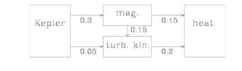
Figure 4.1: Energy budget in a local accretion disc simulation where the turbulence is maintained by the Balbus-Hawley instability. The numbers on the arrows indicate the approximate energy conversion rates in units of $\Omega E_{\rm M}$, where $\Omega$ is the angular velocity and $E_{\rm M}$ is the steady state value of the magnetic energy. (Adapted from Ref. [201].)

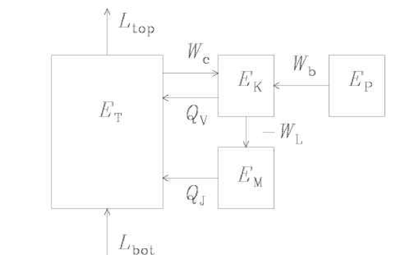
Figure 4.2: Energy budget in a local convection simulation. The dynamo is convectively driven by the luminosity entering from below, giving rise to convection via work done by adiabatic compression, $W_{\rm c}=\int p\bm{\nabla}\cdot\bm{u}\,\mathrm{d}V$, and through work done against the Lorentz force, $W_{\rm L}=\int\bm{u}\cdot(\bm{J}\times\bm{B})\,\mathrm{d}V$. Energy is being fed back from magnetic and kinetic energy to thermal energy via Joule and viscous heating, $Q_{\rm J}$ and $Q_{\rm v}$. Some of the kinetic energy is constantly being exchanged with potential energy $E_{\rm P}$ via $W_{\rm b}=\int\rho\bm{g}\cdot\bm{u}\,\mathrm{d}V$ (adapted from Ref. [203]).

In the case of solar convection the energy for the dynamo comes ultimately from the nuclear reactions in the center of the star. These acts as a source of thermal energy which gets converted into kinetic energy via the convection instability. The corresponding energy diagram for this case is shown in Fig. 4.2. Potential energy does not contribute directly: it only contributes through rearranging the mean density stratification [203].

4.2 Kinematic dynamos

The onset of dynamo action can be studied in the linear approximation, i.e. the velocity field is assumed to be given (kinematic problem). There is in general a critical value of the magnetic Reynolds number above which the magnetic field grows exponentially. A lot of work has been devoted to the question of whether the growth rate can remain finite in the limit $R_{\rm m}\to\infty$ (the so-called fast dynamo problem); see Refs [204, 205, 206] for reviews. Fast dynamos are physically meaningful only until nonlinear effects begin to modify the flow to limit further growth of the field.

In the following we consider two simple examples of a dynamo. Both are slow dynamos, i.e. magnetic diffusion is crucial for the operation of the dynamo. We also discuss the stretch-twist-fold dynamo as a qualitative example of what is possibly a fast dynamo.

4.2.1 The Herzenberg dynamo

In the wake of Cowling’s antidynamo theorem [207] the Herzenberg dynamo [208] played an important role as an early example of a dynamo where the existence of excited solutions could be proven rigorously. The Herzenberg dynamo does not attempt to model an astrophysical dynamo. Instead, it was complementary to some of the less mathematical and more phenomenological models at the time, such as Parker’s migratory dynamo [209] as well as the observational model of Babcock [210], and the semi-observational model of Leighton [211], all of which were specifically designed to describe the solar cycle.

The Herzenberg dynamo is based on the mutual interaction of the magnetic fields produced by two spinning spheres in a conducting medium. In its simplest variant, the axes of the two spheres lie in two parallel planes and have an angle $\varphi$ to each other; see Fig. 4.3, which shows the field vectors from a numerical simulation of the Herzenberg dynamo [212].

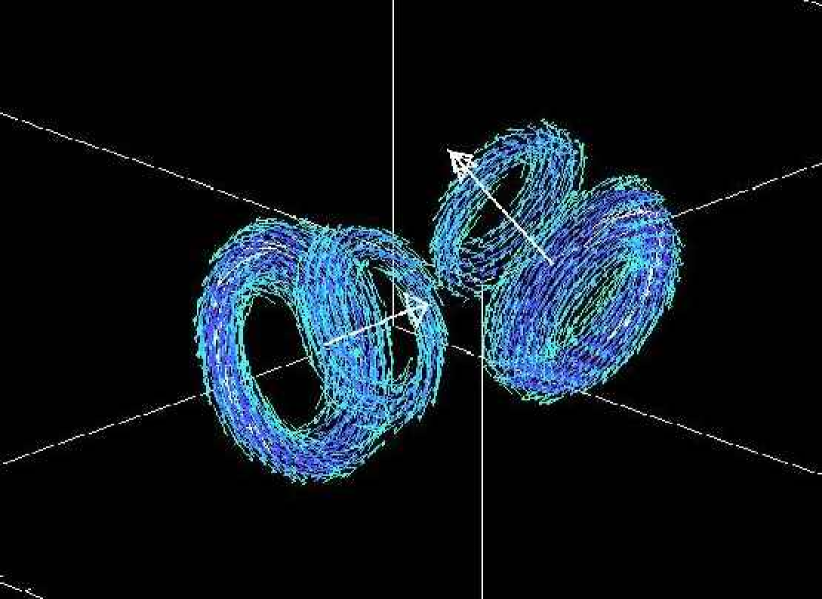
Figure 4.3: Three-dimensional visualization of the magnetic field geometry of the Herzenberg dynamo. $\bm{B}$-vectors are shown when their length exceeds about 25% of the maximum value (adapted from Ref. [212]).

Dynamo action is possible unless the angle $\varphi$ is exactly $0^{\circ}$, $90^{\circ}$, or $180^{\circ}$. For $90^{\circ}<\varphi<180^{\circ}$ nonoscillatory dynamo action is possible. In the limit where the radius of the spheres, $a$, is small compared with their separation $d$, one can expand the field locally in terms of multipoles to lowest order. Defining a magnetic Reynolds number as $R_{\rm m}=\omega d^{2}/\eta$, where $\omega$ is the spin frequency of each of the spheres, the critical magnetic Reynolds number for dynamo action, $R_{\rm crit}$, is found to be [148]

$$R_{\rm crit}^{-2}=-{1\over 4800}\left({a\over d}\right)^{6}\sin\!^{2}\varphi\cos\varphi\quad\mbox{(for $90^{\circ}<\varphi<180^{\circ}$}),$$ (4.3)

which shows that the smallest value of $R_{\rm crit}$ is reached for $\varphi\approx 125^{\circ}$. Critical magnetic Reynolds numbers are several hundreds. However, because $R_{\rm m}$ depends quadratically on $d$, $R_{\rm crit}$ would be only around ten if we were to redefine the magnetic Reynolds number based on some typical wavenumber; see Eq. (3.18). The dynamo works on the principle that each sphere winds up its ambient field, creates thereby a strong toroidal field around itself. Because there is an angle between the two spheres the toroidal field of one sphere acts as a poloidal field for the other sphere. For the toroidal field of each sphere to propagate to the other sphere, a non-zero diffusion is necessary, hence making this dynamo a slow dynamo.

Already back in the sixties, the idea of the Herzenberg dynamo has been verified experimentally [213, 214] using two conducting cylinders embedded in a solid block of the same material. The cylinders were in electric contact with the block through a thin lubricating film of mercury.

The asymptotic theory of Herzenberg [208] assumed that $a/d\ll 1$; for excellent reviews of the Herzenberg dynamo see Refs [148, 215]. Using numerical simulations [212], it has been shown that Eq. (4.3) remains reasonably accurate even when $a/d\approx 1$. These simulations also show that in the range $0^{\circ}<\varphi<90^{\circ}$ dynamo action is still possible, but the solutions are no longer steady but oscillatory; see Ref. [212] for an asymptotic treatment. In the early papers, only steady solutions were sought, which is the reason why no solutions were originally found for $0^{\circ}<\varphi<90^{\circ}$.

4.2.2 The Roberts flow dynamo

In the early years of dynamo theory most examples were constructed and motivated based on what seems physically possible and plausible. An important element of astrophysical dynamos is that the flow is bounded in space and that the magnetic field extends to infinity. Later, and especially in recent years, these restrictions were relaxed in may approaches. One of the first examples is the G. O. Roberts dynamo [216, 217]. The flow depends on only two coordinates, $\bm{U}=\bm{U}(x,y)$, and can be written in the form

$$\bm{U}(x,y)=k_{\rm f}^{-1}\bm{\nabla}\times(\varphi\hat{\mbox{\boldmath$z$}}{})+k_{\rm f}^{-2}\bm{\nabla}\times\bm{\nabla}\times(\varphi\hat{\mbox{\boldmath$z$}}{}),$$ (4.4)

with the stream function $\varphi=\sqrt{2}\,U_{0}\cos k_{x}x\cos k_{y}y$, where $k_{x}=k_{y}=\pi/a$; see Fig. 4.4. This flow is fully helical with $\bm{W}=k_{\rm f}\bm{U}$, were $k_{\rm f}^{2}=k_{x}^{2}+k_{y}^{2}$ and $\bm{W}=\bm{\nabla}\times\bm{U}$. The flow is normalized such that $\langle\bm{U}^{2}\rangle=U_{0}^{2}$. While the flow is only two-dimensional (in the sense that $\bm{U}$ is a function only of $x$ and $y$), the magnetic field must be three-dimensional for all growing solutions (dynamo effect). The field must therefore also depend on $z$.

Figure 4.4: Roberts flow pattern with periodicity $2a$, corresponding to Eq. (4.4) (adapted from Ref. [218]).

Figure 4.5: Critical magnetic Reynolds number, $R_{\rm crit}=U_{0}/(\eta k_{\rm f})_{\rm crit}$, for the Roberts flow as a function of $k_{z}/k_{\rm f}$, where $k_{\rm f}^{2}=k_{x}^{2}+k_{y}^{2}$. The critical magnetic Reynolds number based on $k_{z}$, $R_{{\rm crit},kz}=U_{0}/(\eta k_{z})_{\rm crit}$, has a minimum at $k_{z}\approx 0.34k_{\rm f}\approx 0.48k_{x}$ (dotted line). The case of a squared domain with $k_{x}=k_{y}=k_{z}$, i.e. $k_{z}/k_{\rm f}=1/\sqrt{2}$, is indicated by the vertical dash-dotted line.

The governing equations are homogeneous with coefficients that are independent of $z$ and $t$. The solutions of the kinetic problem can therefore be written in the form

$$\bm{B}(x,y,z,t)={\rm Re}\left[\hat{\bm{B}}_{k_{z}}(x,y)\exp(\mathrm{i}k_{z}z+\lambda t)\right],$$ (4.5)

where $\hat{\bm{B}}_{k_{z}}$ is the eigenfunction, which is obtained by solving the eigenvalue problem

$$\lambda\hat{\bm{A}}_{k_{z}}=\bm{U}\times\hat{\bm{B}}_{k_{z}}+\eta\left(\nabla^{2}-k_{z}^{2}\right)\hat{\bm{A}}_{k_{z}},$$ (4.6)

where $\hat{\bm{B}}_{k_{z}}=\bm{\nabla}\times\hat{\bm{A}}_{k_{z}}+\mathrm{i}\bm{k}_{z}\times\hat{\bm{A}}_{k_{z}}$ is expressed in terms of $\hat{\bm{A}}_{k_{z}}$, which is a mixed representation of the vector potential; in real space the vector potential would be ${\rm Re}\left[\hat{\bm{A}}_{k_{z}}(x,y)\exp(\mathrm{i}k_{z}z+\lambda t)\right]$. In Fig. 4.5 we present critical values of the magnetic Reynolds number as a function of $k_{z}$, obtained by solving Eq. (4.6) numerically as described in Refs [218, 219]. For $k_{z}=k_{x}=k_{y}\approx 0.71k_{\rm f}$, the marginal state ($\lambda=0$) is reached when $R_{\rm crit}\equiv U_{0}/(\eta k_{\rm f})_{\rm crit}\approx 3.90$. The larger the domain in the $z$-direction, the lower is the critical magnetic Reynolds number. However, the critical magnetic Reynolds number based on $k_{z}$, $R_{{\rm crit},kz}=U_{0}/(\eta k_{z})_{\rm crit}$, has a minimum at $k_{z}\approx 0.34k_{\rm f}\approx 0.48k_{x}$ with $R_{{\rm crit},kz}\approx 3.49$; cf. Fig. 4.5.

The horizontally averaged eigenfunction is $\overline{\hat{\bm{B}}}_{k_{z}}=(\mathrm{i},1,0)$, corresponding to a Beltrami wave (see Section 3.7), which has maximum magnetic helicity with a sign that is opposite to that of the flow. In the present case, the kinetic helicity of the flow is positive, so the magnetic and current helicities of the mean field are negative.

The significance of this solution is two-fold. On the one hand, this dynamo is the prototype of any fully helical dynamo capable of generating a large scale field ($k_{z}\ll k_{\rm f}$). On the other hand, it is a simple model of the Karlsruhe dynamo experiment where a similar flow of liquid sodium is generated by an arrangement of pipes with internal ‘spin generators’ making the flow helical. It is also an example of a flow where the generation of the magnetic field can be described in terms of mean field electrodynamics.

Unlike the original Roberts flow dynamo, the flow in the Karlsruhe dynamo experiment is bounded and embedded in free space. Within the dynamo domain, the mean field, $\overline{\hat{\bm{B}}}_{k_{z}}=(\mathrm{i},1,0)$, has only $(x,y)$-components. The field lines must close outside the dynamo domain, giving therefore rise to a dipole lying in the $(x,y)$-plane. Similar fields have long been predicted for rapidly rotating stars [220]. This will be discussed in more detail in Section 11.3.3.

4.3 Fast dynamos: the stretch-twist-fold picture

An elegant heuristic dynamo model illustrating the possibility of fast dynamos is what is often referred to as the Zeldovich ‘stretch-twist-fold’ (STF) dynamo (see Fig. 4.6). This is now discussed in many books [206, 222] and we briefly outline it here, as it illustrates nicely several features of more realistic dynamos.

The dynamo algorithm starts with first stretching a closed flux rope to twice its length preserving its volume, as in an incompressible flow (A$\to$B in Fig. 4.6). The rope’s cross-section then decreases by factor two, and because of flux freezing the magnetic field doubles. In the next step, the rope is twisted into a figure eight (B$\to$C in Fig. 4.6) and then folded (C$\to$D in Fig. 4.6) so that now there are two loops, whose fields now point in the same direction and together occupy a similar volume as the original flux loop. The flux through this volume has now doubled. The last important step consists of merging the two loops into one (D$\to$A in Fig. 4.6), through small diffusive effects. This is important in order that the new arrangement cannot easily undo itself and the whole process becomes irreversible. The newly merged loops now become topologically the same as the original single loop, but now with the field strength scaled up by factor 2.

Figure 4.6: A schematic illustration of the stretch-twist-fold-merge dynamo.

Repeating the algorithm $n$ times, leads to the field in the flux loop growing by factor $2^{n}$, or at a growth rate $\sim T^{-1}\ln 2$ where $T$ is the time for the STF steps. This makes the dynamo potentially a fast dynamo, whose growth rate does not decrease with decreasing resistivity. Also note that the flux through a fixed ‘Eulerian surface’ grows exponentially, although the flux through any lagrangian surface is nearly frozen; as it should be for small diffusivities.

The STF picture illustrates several other features: first we see that shear is needed to amplify the field at step A$\to$B. However, without the twist part of the cycle, the field in the folded loop would cancel rather than add coherently. To twist the loop the motions need to leave the plane and go into the third dimension; this also means that field components perpendicular to the loop are generated, albeit being strong only temporarily during the twist part of the cycle. The source for the magnetic energy is the kinetic energy involved in the STF motions.

Most discussions of the STF dynamo assume implicitly that the last step of merging the twisted loops can be done at any time, and that the dynamo growth rate is not limited by this last step. This may well be true when the fields in the flux rope are not strong enough to affect the motions, that is, in the kinematic regime. However as the field becomes stronger, and if the merging process is slow, the Lorentz forces due to the small scale kinks and twists will gain in importance compared with the external forces associated with the driving of the loop as a whole. This may then limit the efficiency of the dynamo.

Indeed, the growing complexity of the field, in the repeated application of the STF process, without the merging, can be characterized particularly by the evolution of the magnetic helicity spectrum. This is discussed for example in Ref. [223], where it is pointed out that the repeated application of the STF cycle (with the same sense for the twist part of the cycle), under flux freezing, leads to both a large scale writhe helicity associated with the repeated crossings of the flux tube, and oppositely signed twist helicity at much smaller scales. If one does not destroy this small scale structure by diffusion, then the Lorentz forces associated with these structures will interfere with the STF motions. A somewhat similar situation holds for the mean field turbulent dynamos, where we will find oppositely signed (almost equal strength) helicities being generated by the motions on different scales. In that case we also find the dynamo to be eventually resistively limited, when there is strict helicity conservation.

In this context one more feature deserves mentioning: if in the STF cycle one twists clockwise and folds, or twists counter-clockwise and folds one will still increase the field in the flux rope coherently. However, one would introduce opposite sense of writhe in these two cases, and so opposite internal twists. So, although the twist part of the cycle is important for the mechanism discussed here, the sense of twist can be random and does not require net helicity. This is analogous to a case when there is really only a small scale dynamo, but one that requires finite kinetic helicity density locally. We should point out, however, that numerical simulations [224] have shown that dynamos work and are potentially independent of magnetic Reynolds number even if the flow has zero kinetic helicity density everywhere.

If the twisted loops can be made to merge efficiently, the saturation of the STF dynamo would probably proceed differently. For example, the field in the loop may become too strong to be stretched and twisted, due to magnetic curvature forces. Another interesting way of saturation is that the incompressibility assumed for the motions may break down; as one stretches the flux loop the field pressure resists the decrease in the loop cross-section, and so the fluid density in the loop tends to decrease as one attempts to make the loop longer. (Note that it is $B/\rho$ which has to increase during stretching.) The STF picture has inspired considerable work on various mathematical features of fast dynamos and some of this work can be found in the book by Childress and Gilbert [206] which in fact has STF in its title!

4.4 Fast ABC-flow dynamos

ABC flows are solenoidal and fully helical with a velocity field given by

$$\bm{U}=\pmatrix{C\sin kz+B\cos ky\cr A\sin kx+C\cos kz\cr B\sin ky+A\cos kx}.$$ (4.7)

When $A$, $B$, and $C$ are all different from zero, the flow is no longer integrable and has chaotic streamlines. There is numerical evidence that such flows act as fast dynamos [225]. The magnetic field has very small net magnetic helicity [159, 223]. This is a general property of any dynamo in the kinematic regime and follows from magnetic helicity conservation, as will be discussed later (Section 8.2 and Fig. 8.2). Even in a nonlinear formulation of the ABC flow dynamo problem, where the flow is driven by a forcing function similar to Eq. (4.7) the net magnetic helicity remains unimportant [226, 227]. This is however not surprising, because the development of net magnetic helicity requires sufficient scale separation, i.e. the wavenumber of the flow must be large compared with the smallest wavenumber in the box ($k=k_{1}\equiv 2\pi/L$, where $L$ is the size of the box). If this is not the case, helical MHD turbulence behaves similarly to nonhelical turbulence [254]. A significant scale separation also weakens the symmetries associated with the flow and the field, and leads to a larger kinematic growth rate, more compatible with the turnover time scale [228]. These authors also find that the cigar-like magnetic field structures which develop in canonical $A=B=C$ flows with stagnation points, are replaced by more ribbon like structures in flows without such stagnation points.

Most of the recent work on nonlinear ABC flow dynamos has focused on the case with small scale separation and, in particular, on the initial growth and possible saturation mechanisms [229]. In the kinematic regime, these authors find a near balance between Lorentz work and Joule dissipation. The balance originates primarily from small volumes where the strong magnetic flux structures are concentrated. The net growth of the magnetic energy comes about through stretching and folding of relatively weak field which occupies most of the volume. The mechanism for saturation could involve achieving a local pressure balance in these strong field regions [230].

5 Small scale turbulent dynamos

Dynamos are often divided into small scale and large scale dynamos. Large scale dynamos are those responsible for the solar cycle, for example. They show large scale spatial coherence and, in the case of the sun, they also show long-term temporal order in the sense of the 11 year cycle, i.e. much longer than the time scale of the turbulent motions. Small scale dynamos produce magnetic fields that are correlated on scales of the order of or smaller than the energy carrying scale of the turbulence. In the literature such dynamos are sometimes also referred to as ‘fluctuation dynamos’. Nonhelical turbulent flows can act as small scale dynamos, while flows with significant amounts of kinetic helicity act as large scale dynamos. Inhomogeneous and anisotropic flows (e.g. shear flows) are potential candidates for producing large scale dynamo action. Of course, there may not be a clear boundary between small and large scale dynamos and indeed the two may interact Section 5.6.

Small scale dynamos are potentially important for several reasons. First, they typically have larger growth rates than large scale dynamos. The question now arises as to what effect this rapidly generated magnetic ‘noise’ has on the large scale dynamo action. Further, there could be physical settings where large scale dynamos do not work, like in clusters of galaxies or in elliptical galaxies where rotation effects are negligible and hence any turbulent flows lack helicity and persistent shear. In such systems, turbulence may still lead to small scale dynamo action and generate magnetic fields. Whether such fields are coherent enough to lead to the observed cluster rotation measures, for example, is an important question to settle.

5.1 General considerations

In a turbulent flow fluid particles random walk away from each other with time. A magnetic field line frozen into the fluid (assuming large $R_{\rm m}$) will then also lengthen by this random stretching. This leads to an increase in $B/\rho$ and for flows with $\rho\approx{\rm const}{}$, the magnetic field will be amplified. The lengthening of the field line in a given direction also leads to a decrease in its scale in the directions perpendicular to the stretching. As the field strength increases, the scale of individual field structures decreases and the Ohmic dissipation increases, until it roughly balances the growth due to random stretching. What happens after this? This question of the long term behavior of the magnetic field in a turbulent flow was first raised by Batchelor [231]. He argued on the basis of the analogy of the induction equation to the equation for vorticity, that the field will grow exponentially if the magnetic Prandtl number is larger than unity. This argument is dubious and the possibility of dynamo action in turbulent flows that lack helicity was first elucidated in a decisive manner by Kazantsev [13] for a special kind of flow. Numerical simulations of turbulent flows also show invariably that dynamo action can occur for forced turbulence. We first discuss the Kazantsev dynamo model and then present some results from simulations of turbulent flows.

5.2 Kazantsev theory

Kazantsev considered a velocity field, $\bm{v}$, which is an isotropic, homogeneous, gaussian random field with zero mean and also, more importantly, which is $\delta$-correlated in time. [We use the symbol $\bm{v}$ instead of $\bm{U}$ to emphasize that $\bm{v}$ is not the solution of the momentum equation (3.41).] The two point spatial correlation function of the velocity field can be written as $\langle v_{i}({\bm{x}},t)v_{j}({\bm{y}},s)\rangle=T_{ij}(r)\delta(t-s)$, where

$$T_{ij}(r)=\left(\delta_{ij}-{r_{i}r_{j}\over r^{2}}\right)T_{\rm N}(r)+{r_{i}r_{j}\over r^{2}}T_{\rm L}(r).$$ (5.1)

Here $\langle\cdot\rangle$ denotes averaging over an ensemble of the stochastic velocity field $\bm{v}$, $r=|\bm{x}-\bm{y}|$, $r_{i}=x_{i}-y_{i}$ and we have written the correlation function in the form appropriate for a statistically isotropic and homogeneous tensor (cf. Section 34 of Ref. [232]). Note that homogeneity implies that the two point correlation function depends only on $\bm{x}-\bm{y}$. Together with isotropy this also implies that the correlation tensor can only contain terms proportional to $\delta_{ij}$, $r_{i}r_{j}$ and $\epsilon_{ijk}$ and the functions multiplying these tensors depend only on $r$. $T_{\rm L}(r)$ and $T_{\rm N}(r)$ are the longitudinal and transverse correlation functions for the velocity field. (The helical part of the velocity correlations is assumed to be zero in this section; see however Section 5.6.) If $\bm{v}$ is assumed to be divergence free, then $T_{\rm N}$ is related to $T_{\rm L}$ via

$$T_{\rm N}={1\over 2r}{\partial\over\partial r}\left[r^{2}T_{\rm L}(r)\right],$$ (5.2)

with

$$T_{\rm L}(0)={\textstyle{1\over 3}}\int_{0}^{t}\langle\bm{v}(t)\cdot\bm{v}(t^{\prime})\rangle\;\mathrm{d}t^{\prime}.$$ (5.3)

We will see in the next section that $T_{\rm L}(0)$ is actually the turbulent diffusion coefficient for the mean field.

5.2.1 Kazantsev equation in configuration space

The stochastic induction equation can now be converted into equations for the various moments of the magnetic field. Assume that there is no mean field or first moment, and that the magnetic correlation has the same symmetries as the flow; i.e. it is isotropic and homogeneous. Then its equal time, two point correlation is given by $\left<B_{i}({\bm{x}},t)B_{j}({\bm{y}},t)\right>=M_{ij}(r,t)$, where

$$M_{ij}=\left(\delta_{ij}-{r_{i}r_{j}\over r^{2}}\right)M_{\rm N}(r,t)+{r_{i}r_{j}\over r^{2}}M_{\rm L}(r,t),$$ (5.4)

and $M_{\rm L}(r,t)$ and $M_{\rm N}(r,t)$ are, respectively, the longitudinal and transversal correlation functions of the magnetic field. Since $\bm{\nabla}\cdot\bm{B}=0$,

$$M_{\rm N}={1\over 2r}{\partial\over\partial r}\left(r^{2}M_{\rm L}\right).$$ (5.5)

Kazantsev derived an equation for $M_{\rm L}(r,t)$ by deriving the equation for the $k$-space magnetic spectrum using diagram techniques, and transforming the resulting integro-differential equation in $k$-space into a differential equation in $r$-space. This $k$-space equation was also derived by Kraichnan and Nagarajan [233]. Subsequently, Molchanov et al. [234, 235] derived this equation directly in $r$-space by the Wiener path integral method. We present a simple derivation of the Kazantsev equation in the more general case of helical turbulence in Appendix A, following the method outlined in Subramanian [236]. For a nonhelical random flow we have

$${\partial M_{\rm L}\over\partial t}={2\over r^{4}}{\partial\over\partial r}\left[r^{4}\eta_{\rm T}(r){\partial M_{\rm L}\over\partial r}\right]+GM_{\rm L},$$ (5.6)

where $\eta_{\rm T}(r)=\eta+\eta_{\rm t}(r)$ is the sum of the microscopic diffusivity, $\eta$, and an effective scale-dependent turbulent magnetic diffusivity $\eta_{\rm t}(r)=T_{\rm L}(0)-T_{\rm L}(r)$. The term $G=-2(T_{\rm L}^{\prime\prime}+4T_{\rm L}^{\prime}/r)$, where primes denote $r$ derivatives, describes the rapid generation of magnetic fluctuations by velocity shear and the potential existence of a small scale dynamo (SSD) independent of any large scale field; see the book by Zeldovich et al. [222] and references therein.

One can look for eigenmode solutions to Eq. (5.6) of the form $\Psi(r)\exp(2\Gamma t)=r^{2}\sqrt{\eta_{\rm T}}M_{\rm L}$. This transforms Eq. (5.6) for $M_{\rm L}(r,t)$, into a time independent, Schrödinger-type equation, but with a variable (and positive) mass,

$$-\Gamma\Psi=-\eta_{\rm T}{d^{2}\Psi\over dr^{2}}+U_{0}(r)\Psi.$$ (5.7)

The ‘potential’ is

$$U_{0}(r)=T_{\rm L}^{\prime\prime}+{2\over r}\,T_{\rm L}^{\prime}+{1\over 2}\,\eta_{\rm T}^{\prime\prime}-{(\eta_{\rm T}^{\prime})^{2}\over 4\eta_{\rm T}}+{2\over r^{2}}\,\eta_{\rm T}$$ (5.8)

for a divergence free velocity field. The boundary condition is $\Psi\to 0$ for $r\to 0,\infty$. Note that $U_{0}\to 2\eta/r^{2}$ as $r\to 0$, and since $T_{\rm L}(r)\to 0$ as $r\to\infty$, it follows that $U_{0}\to 2[\eta+T_{\rm L}(0)]/r^{2}$ as $r\to\infty$. The possibility of growing modes with $\Gamma>0$ is obtained, if one can have a potential well with $U_{0}$ sufficiently negative in some range of $r$. This allows for the existence of bound states with ‘energy’ $E=-\Gamma<0$. The solutions to the Kazantsev equation for various forms of $T_{\rm L}(r)$ have been studied quite extensively by several authors [13, 222, 236, 237, 238, 239, 240, 241, 242].

Suppose we have random motions correlated on a single scale $L$, with a velocity scale $V$. Define the magnetic Reynolds number $R_{\rm m}=VL/\eta$. (Here we define $R_{\rm m}$ using the correlation scale $L$ instead of $L/2\pi$ since this appears most natural, and is also commonly used, in real space treatments of the SSD.) Such a random flow may arise if the fluid is highly viscous, and it will also be relevant for the viscous cut-off scale eddies in Kolmogorov turbulence. Then one finds that there is a critical $R_{\rm m}=R_{\rm crit}$, so that for $R_{\rm m}>R_{\rm crit}$, the potential $U_{0}$ allows for the existence of bound states. For $R_{\rm m}=R_{\rm crit}$, one has $\Gamma=0$, and this marginal stationary state is the ‘zero’ energy eigenstate in the potential $U_{0}$. The value of $R_{\rm crit}$ one gets ranges between $30-60$, depending on the assumed form of $T_{\rm L}(r)$ [236, 237, 238]. (This $R_{\rm crit}$ corresponds to a value $30/2\pi-60/2\pi$ if we were to use the corresponding wavenumber $2\pi/L$ to define $R_{\rm m}$.) For $R_{\rm m}>R_{\rm crit}$, $\Gamma>0$ modes of the SSD can be excited, and the fluctuating field that is correlated on a scale $L$ grows exponentially on the corresponding ‘eddy’ turnover time scale. For example, suppose one adopts $T_{\rm L}(r)=(VL/3)(1-r^{2}/L^{2})$ for $r<L$, and zero otherwise, as appropriate for a single scale flow (or the flow below the viscous cut-off). Then, a WKBJ analysis [236] gives the growth rate for the fastest growing mode as $\Gamma={5\over 4}V/L-{\cal O}((\ln R_{\rm m})^{-2})$.

To examine the spatial structure for various eigenmodes of the small scale dynamo, it is more instructive to consider the function

$$w(r,t)=\langle\bm{B}({\bm{x}},t)\cdot\bm{B}({\bm{y}},t)\rangle={1\over r^{2}}{\partial\over\partial r}\left(r^{3}M_{\rm L}\right),\quad\mbox{$r=|\bm{x}-\bm{y}|$},$$ (5.9)

which measures the ensemble average of the dot product of the fluctuating field at two locations, with $w(0,t)=\langle\bm{B}^{2}\rangle$. We have $\int_{0}^{\infty}w(r)r^{2}dr=\int_{0}^{\infty}(r^{3}M_{\rm L})^{\prime}=0$, since $M_{\rm L}$ is regular at the origin and vanishes faster than $r^{-3}$ as $r\to\infty$. Therefore the curve $r^{2}w(r)$ should have zero area under it. Since $w(0,t)=\langle\bm{B}^{2}\rangle$, $w$ is positive near the origin. Therefore, $\bm{B}$ points in the same direction for small separation. As one goes to larger values of $r$, there must be values of $r$, say $r\sim d$, where $w(r)$ becomes negative. For such values of $r$, the field at the origin and at a separation $d$ are, on the average, pointing in opposite directions. This can be interpreted as indicating that the field lines, on the average, are curved on the scale $d$.

For the growing modes of the small scale dynamo, one finds [236, 237, 238, 239, 240] that $w(r)$ is strongly peaked within a region $r=r_{d}\approx LR_{\rm m}^{-1/2}$ about the origin, for all the modes, and for the fastest growing mode, changes sign across $r\sim L$ and rapidly decays with increasing $r/L$. The scale $r_{d}$ is in fact the diffusive scale determined by the balance of rate of the Ohmic decay, $\eta/r_{d}^{2}$, and the growth rate $V/L$ due to random shearing. (Note for the single scale flow one has linear shear at small scales, and hence a scale-independent shearing rate.) Detailed asymptotic solutions for $w(r)$ have been given in Ref. [238] and a WKBJ treatment can also be found in Ref. [236]. A physical interpretation of this correlation function [222, 238, 239] is that the small scale field in the kinematic regime is concentrated in structures with thickness $r_{d}$ and curved on a scale up to $\sim L$. How far such a picture holds in the nonlinear regime is still matter of investigation (see below).

The small scale dynamo in Kolmogorov turbulence can be modeled [236, 240] by adopting $T_{\rm L}(r)={\textstyle{1\over 3}}VL[1-(r/L)^{4/3}]$ in the inertial range $l_{d}<r<L$, a form suggested in Ref. [243]. Here $L$ is the outer scale and $l_{d}\approx L\mbox{Re}^{-3/4}$ is the viscous cut-off scale of the turbulence, where $\mbox{Re}=VL/\nu$ is the fluid Reynolds number. For Kolmogorov turbulence, the eddy velocity at any scale $l$, is $v_{l}\propto l^{1/3}$, in the inertial range. So the scale dependent diffusion coefficient scales as $v_{l}l\propto l^{4/3}$. This scaling, also referred to as Richardson’s law, is the motivation for the above form $T_{\rm L}(r)$. Also, in order to ensure that $T_{L}^{\prime}(0)=0$, $T_{L}$ is continued from its value at $r=l_{d}$ to zero, and was taken to be zero for $r>L$. (The exact form of the continuation has little effect on the conclusions.) In the inertial range the potential then has the scale invariant form,

$$U={v_{l}\over 3l}\left[-{8\over 9}\left({r\over l}\right)^{-2/3}-{(4/9)(r/l)^{2/3}\over 3/R_{\rm m}(l)+(r/l)^{4/3}}+{6\over R_{\rm m}(l)}\left({L^{2}\over r^{2}}\right)\right],$$ (5.10)

where $R_{\rm m}(l)=v_{l}l/\eta=R_{\rm m}(l/L)^{3/4}$ is the magnetic Reynolds number associated with a scale $l$. Note that the potential $U$ (not to be confused with the velocity $\bm{U}$) has the same form at any scale $l$, with $R_{\rm m}(l)$ appropriate to that scale. This suggests that conclusions about the excitation conditions can be applied separately at different scales, $l$, provided we use the corresponding velocity scale $v_{l}$ and Reynolds number $R_{\rm m}(l)$ appropriate to the scale $l$. For example, the condition for excitation of small scale dynamo modes which are concentrated at a scale $l$, is also $R_{\rm m}(l)=R_{\rm crit}\gg 1$.

Note that $R_{\rm m}(l)$ decreases as one goes to smaller scales, and so the small scale dynamo will be first excited when the magnetic Reynolds number at the outer scale satisfies $R_{\rm m}(L)>R_{\rm crit}$. For Kolmogorov turbulence described by the above $T_{\rm L}(r)$ it was estimated [236] using a WKBJ analysis that $R_{\rm crit}\sim 60$. Also, the marginal mode which has zero growth rate, in this case, has $w(r)$ peaked within $r\sim L/R_{\rm m}^{3/4}$. This different scaling can be understood as arising due to the fact that the shearing rate now is $(V/L)(r/L)^{-2/3}$ at any scale $r$ in the inertial range. For the marginal mode this is balanced by dissipation at $r=r_{d}$ which occurs at a rate $\eta/r_{d}^{2}$.

In Kolmogorov turbulence, the cut-off scale eddies have $R_{\rm m}(l_{d})=P_{\rm m}$, i.e. the cutoff-scale magnetic Reynolds number is equal to the magnetic Prandtl number. So, if $P_{\rm m}>R_{\rm crit}$ these eddies are themselves capable of small scale dynamo action. The fastest growing modes then have a growth rate $\sim v_{d}/l_{d}$, which is equal to the eddy turnover time associated with the cut-off scale eddies, a time scale much smaller than the turnover time of outer scale eddies. Also, for the fastest growing mode $w(r)$ is peaked about a radius corresponding to the diffusive scales associated with these eddies, and changes sign at $r\sim l_{d}$.

We have taken the scale-dependent turbulent diffusion coefficient $T_{\rm L}(0)-T_{\rm L}(r)\propto r^{n}$ with $n=4/3$ to model Kolmogorov turbulence. The index $n$ measures how ‘rough’ the velocity field is, with $n=2$ corresponding to a smooth velocity field. It turns out that for growing modes one requires $n>1$ at least [13]. Also, in a small $P_{\rm m}$ flow the closer $n$ is to unity, the larger could be the critical $R_{\rm m}$ needed to excite the small scale dynamo [244]. This may be of relevance for understanding the results of small $P_{\rm m}$ dynamo simulations that are described below (Section 5.5).

5.2.2 Kazantsev dynamo in Fourier space

It is instructive to study the Kazantsev problem in Fourier space. In $k$ space the differential equation (5.6) becomes an integro-differential equation for the magnetic spectrum $M(k,t)$, which is in general difficult to solve. However, if the magnetic spectrum is peaked on scales much smaller than the flow, as is the case for small fluid Reynolds number (large $P_{\rm m}$) flows, one can provide an approximate treatment for the large $k$ regime, $k\gg k_{\rm f}$. Here $k_{\rm f}$ is the forcing scale in case of a single scale random flow, or the viscous scale in case of Kolmogorov turbulence (assuming that eddies at the cut-off scale can also induce dynamo action). In this large $k\gg k_{\rm f}$ limit the Kazantsev equation becomes [143]

$${\partial M\over\partial t}={\gamma\over 5}\left(k^{2}{\partial^{2}M\over\partial k^{2}}-2k{\partial M\over\partial k}+6M\right)-2\eta k^{2}M,$$ (5.11)

where $\gamma=-(1/6)[\nabla^{2}T_{ii}(r)]_{r=0}$, is a measure of the rate of shearing by the flow. In terms of $T_{\rm L}$, we have $\gamma=7T_{\rm L}^{\prime\prime}(0)+8T^{\prime}_{\rm L}(0)/r$. The evolution of the magnetic spectrum was analyzed in some detail in Ref. [143], and is summarized nicely in Ref. [245].

Suppose the initial magnetic spectrum is peaked at some $k=k^{\prime}\ll k_{\rm f}R_{\rm m}^{1/2}$, i.e. at a wavenumber much smaller than the resistive wavenumber, then the amplitude of each Fourier mode grows exponentially in time at the rate ${3\over 4}\gamma$. Meanwhile, the peak of excitation moves to larger $k$, with $k_{\rm peak}=k^{\prime}\exp({3\over 5}\gamma t)$, leaving behind a power spectrum $M(k)\propto k^{3/2}$. These features can of course be qualitatively understood as due to the effects of random stretching. Once the peak reaches the resistive scale, one has to solve again an eigenvalue problem to determine the subsequent evolution of $M(k,t)$. Substituting $M(k,t)=\exp^{\lambda\gamma t}\Phi(k/k_{\eta})$, where $k_{\eta}=(\gamma/10\eta)^{1/2}$, into (5.11) and demanding that $\Phi\to 0$ as $k\to\infty$, one gets the solution [245]

$$\Phi(k/k_{\eta})={\rm const}{}\times k^{3/2}K_{\nu(\lambda)}(k/k_{\eta}),\quad\nu(\lambda)=\sqrt{5(\lambda-{\textstyle{3\over 4}})}.$$ (5.12)

Here $K_{\nu}$ is the Macdonald function and the eigenvalue $\lambda$ must be determined from the boundary condition at small $k$. This is a bit more tricky in the $k$-space analysis since the equations were simplified by taking the large $k$ limit; fortunately the results seem independent of the exact form of the boundary condition at small $k$ in the large $R_{\rm m}$ limit. In Ref. [245] a zero flux boundary condition is imposed at some $k=k_{*}\ll k_{\eta}$ and it is shown that this fixes $\lambda\approx 3/4$ and $\nu\approx 0$. In case we adopt $T_{\rm L}(r)={\textstyle{1\over 3}}VL(1-r^{2}/L^{2})$, for $r<L$ and zero otherwise, one gets $\gamma={5\over 3}V/L$ and so the growth rate is $\Gamma={3\over 4}\gamma={5\over 4}V/L$, which agrees with the WKBJ analysis of the Kazantsev equation obtained in Section 5.2.1. We also get $1/k_{\eta}=\sqrt{6}LR_{\rm m}^{-1/2}$ which is of the same order as expected for the diffusive scale $r_{d}$ in the real-space treatment.

We show in Figs. 5.1 and 5.2 the time evolution of the magnetic spectrum from simulations which are described in detail later. One important difference between simulations and the picture described above arises due to the presence of power (however small) in the initial spectrum, at the resistive scale. This leads to the magnetic spectrum extending to the resistive scale, and locking onto an eigenfunction right from the early stages of evolution, as can be seen in Fig. 5.1. We also show the corresponding time evolution for a high $P_{\rm m}$ simulation, which represents more closely the SSD for when the kinetic spectrum is peaked on a single scale; see Fig. 5.2

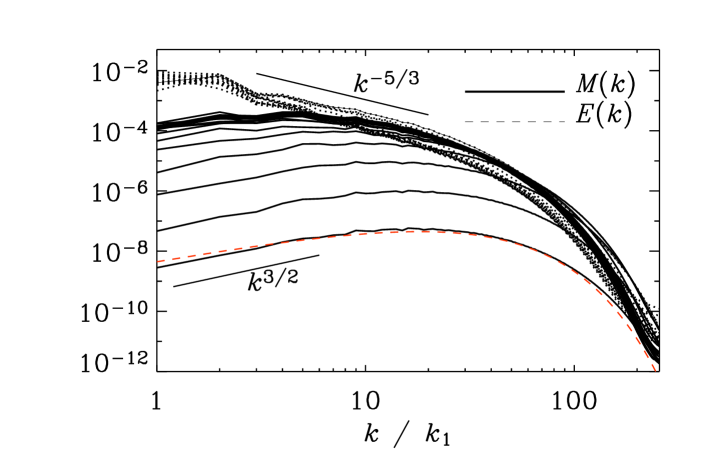
Figure 5.1: Magnetic and kinetic energy spectra from a nonhelical turbulence simulation with $P_{\rm m}=1$. The kinetic energy is indicated as a dashed line (except for the first time displayed where it is shown as a thin solid line). At early times the magnetic energy spectrum follows the $k^{3/2}$ Kazantsev law [the dashed line gives the fit to Eq. (5.12)], while the kinetic energy shows a short $k^{-5/3}$ range. The Reynolds number is $u_{\rm rms}/(\nu k_{\rm f})\approx 600$ and $512^{3}$ meshpoints were used [254]. The time difference between the spectra is about $14\,(k_{\rm f}u_{\rm rms})^{-1}$.

Figure 5.2: Magnetic and kinetic energy spectra from a nonhelical turbulence simulation with $P_{\rm m}=50$. The kinetic energy is indicated as a dotted line (except for the first time displayed where it is shown as a thin solid line). The magnetic spectrum for the last time is shown as a thick line. The Reynolds number is $u_{\rm rms}/(\nu k_{\rm f})\approx 80$, and the magnetic Reynolds number is $u_{\rm rms}/(\eta k_{\rm f})\approx 4000$ and $512^{3}$ meshpoints were used. Like in Fig. 5.1, the time difference between the spectra is about $14\,(k_{\rm f}u_{\rm rms})^{-1}$. At the end of the run the field is still not completely saturated.

5.2.3 Further results on the Kazantsev dynamo

A number of other interesting results have been found for the Kazantsev problem, particularly for the case of a single scale flow. In this case one can approximate the velocity to be a linear random shear flow. In the regime when the field has not yet developed small enough scales, resistivity is unimportant and one can assume the field to be frozen into the flow. The result of such passive random advection is that the magnetic field strength develops a log-normal probability distribution function (PDF) [246, 247]. This log-normal form for the PDF of $B$ can be understood from the induction equation without the diffusion term $\dot{B}_{i}=B_{j}u_{i,j}$ where the time derivative is a lagrangian derivative. Since the RHS is linear in $B_{i}$ and is multiplied by a constant random matrix $u_{i,j}$, the “gaussianity” of log$B$ is expected from the central limit theorem. This implies that the magnetic field becomes highly intermittent. To what extent this PDF is altered by resistivity is examined in Ref. [248]. They find that even when resistivity is included, the field is still intermittent and may be thought of as being concentrated into narrow strips.

This seems to be also borne out by a study of the behavior of higher order $k$-space correlators [249]. By examining their late time evolution, these authors find that the log-normality of the magnetic field PDF persists in the dissipative regime. An interpretation of their $k$-space scalings, suggests that the magnetic structures in physical space could look like ‘ribbons’ with the field directed along these ribbons. Recent numerical work [250], however, finds that even in the kinematic regime, the PDF of $|\bm{B}|$ changes character, perhaps due to having a finite box in the simulation.

Motivated by the need to understand the eventual nonlinear saturation of the small scale dynamo, work has been done by looking at the statistical properties of the Lorentz force, in particular the component $\bm{B}\cdot\bm{\nabla}\bm{B}$ [245, 247, 251]. The idea is that in an incompressible flow, the effects of the Lorentz force will be dominated by the magnetic curvature rather than the magnetic pressure gradient. (Note that although the magnetic pressure forces may be much larger, they are largely balanced by thermal pressure gradients in the incompressible limit.) In Ref. [247] it was shown that though both magnetic energy and mean-square curvature of field lines grow exponentially, the field strength and the curvature are anti-correlated. Thus, regions of strong field are nearly straight, while sharply curved fields are relatively weak. Such a result was in fact found earlier in simulations of dynamo generation of magnetic fields due to convection [203, 252]. In these simulations the magnetic field was found to be intermittent with relatively stronger field concentrated in structures which are relatively straight. Furthermore, the saturation of the dynamo was traced back to the component of $\bm{B}\cdot\bm{\nabla}\bm{B}$ that is perpendicular to the direction of the field; its field-aligned component (i.e. the tension force) was found to be unimportant for saturation [253].

The anti-correlation between the field strength and the curvature is interpreted by [245, 247] as showing that the field lies in folds, which are curved on the flow scale and with rapid reversals on the diffusive scale. To what extent the small scale dynamo generated field is indeed structured in this way is still a matter of debate (see below). Also, one should keep in mind that all the above semi-analytic results on the structure of the field pertain to the kinematic regime. The recent simulations of Haugen et al. [254], discussed in Section 5.4, show occasional field reversals, but such events occupy only a small part of the volume.

5.3 Saturation of the small scale dynamo

How does the small scale dynamo saturate? The answer to this question will be crucial to understanding both the effect of the small scale dynamo generated fields on the large scale dynamo, as well of the relevance of these fields to explain say cluster fields. From the discussion of the kinematic regime, we saw that the field would become intermittent and also concentrated into structures whose thickness, in at least one dimension, is the resistive scale. However nonlinear effects may intervene to alter this kinematic result. There have been a number of attempts to model the nonlinear saturation of the small scale dynamo, none of which are entirely compelling. We discuss these below.

Some effects of the growing magnetic field can arise just due to plasma phenomena like ambipolar drift in a partially ionized gas [240], anisotropic viscosity [255] or collisionless damping [256]. For example, collisionless processes can become important on scales smaller than the ion mean free path and could prevent the magnetic field from being concentrated below such a scale [256]. Ambipolar diffusion is particularly relevant in the galactic context, where there could be a significant neutral component to the interstellar medium. It changes the effective diffusivity by adding an ambipolar diffusion component [236, 240]; see Section 3.8.2 and Appendix A. The effective magnetic Reynolds number of the interstellar medium, taking ambipolar diffusion into account, decreases from about $3\times 10^{19}$ to $R_{\rm AD}\sim 10^{6}$ [240], as the field grows to microgauss strengths. This will then lead to an important increase of the effective diffusive scale which, due to nonlinear ambipolar drift, will become of order $L/R_{\rm AD}^{1/2}\sim 10^{-3}L$. However, since $R_{\rm AD}\gg R_{\rm crit}$, the small scale dynamo does not saturate due to this mechanism.

5.3.1 Saturation via artificial nonlinear drifts

The above discussion of ambipolar drift motivates a nonlinear model problem which may give hints as to how the small scale dynamo can in principle saturate even in a fully ionized gas [257]. Suppose one assumes that, as the magnetic field grows and the Lorentz force pushes on the fluid, the fluid instantaneously responds by developing an additive ‘drift’ component to the velocity, where the drift is proportional to the Lorentz force. The model velocity in the induction equation is then $\bm{u}=\bm{v}+\bm{v}_{\rm N}$, i.e. the sum of an externally prescribed stochastic field $\bm{v}$, and a drift component $\bm{v}_{\rm N}=a\bm{J}\times\bm{B}$. For ambipolar drift, $a$ would be related to the properties of the partially ionized gas. Suppose we adopt instead $a=\tau/\rho$, where $\tau$ is some response (or correlation) time, treated as a phenomenological free parameter and $\rho$ is the fluid density. This gives a model problem, where the nonlinear effects of the Lorentz force are taken into account as simple modification of the velocity field. (Note that in reality it is the acceleration and not the velocity which is proportional to the Lorentz force. Nevertheless the above model provides a useful toy problem for examining the nonlinear saturation effects, especially if the correlation time $\tau$ is small compared to the Alfvén time.) Adding a velocity contribution proportional to the Lorentz force of course also leads to a problem of closure, since in the equation for $M_{\rm L}$, the nonlinear drift term brings in a fourth order magnetic correlation. In Ref. [236, 257] a gaussian closure is assumed (cf. Appendix A).

The backreaction in the form of a nonlinear drift then simply replaces $\eta$ by an effective time-dependent $\eta_{\rm D}=\eta+2aM_{\rm L}(0,t)$ in the $\eta_{\rm T}(r)$ term of Eq. (5.6) [257] (cf. Appendix A). We thus obtain

$$\frac{\partial M_{\rm L}}{\partial t}=\frac{2}{r^{4}}\frac{\partial}{\partial r}\left[r^{4}\eta_{\rm T}(r)\frac{\partial M_{\rm L}}{\partial r}\right]+GM_{\rm L}+K,$$ (5.13)

$$K(r,t)=4aM_{\rm L}(0,t)\frac{1}{r^{4}}\frac{\partial}{\partial r}\left(r^{4}\frac{\partial M_{\rm L}}{\partial r}\right).$$ (5.14)

Define an effective magnetic Reynolds number (just like $R_{\rm AD}$), for fluid motions on scale $L$, by $R_{\rm D}(t)=VL/\eta_{\rm D}(t)$. Then, as the energy density in the fluctuating field, say $E_{\rm M}(t)={\textstyle{3\over 2}}M_{\rm L}(0,t)$, increases, $R_{\rm D}$ decreases. In the final saturated state, with $\partial M_{\rm L}/\partial t=0$ (obtained, say, at time $t_{s}$), $M_{\rm L}$, and hence the effective $\eta_{\rm D}$ in Eq. (5.13) become independent of time. Solving for this stationary state then becomes identical to solving for the marginal (stationary) mode of the kinematic problem, except that $R_{\rm m}$ is replaced by $R_{\rm D}(t_{s})$. The final saturated state is then the marginal eigenmode which one obtains when $E_{\rm M}$ has grown (and $R_{\rm D}$ decreased) such that $R_{\rm D}(t_{s})=VL/[\eta+2aM_{\rm L}(0,t_{s})]=R_{\rm crit}\sim 30$–$60$ (depending on the nature of the velocity field). Also, for this saturated state we predict that $w(r)$ is peaked within a region $r\approx L(R_{\rm crit})^{-1/2}$ about the origin, changes sign across $r\sim L$, and then rapidly decays for larger $r/L$. Further, from the above constraint it follows that $M_{\rm L}(0,t_{s})=vL/(2aR_{\rm crit})$, where we have assumed $\eta\ll 2aM_{\rm L}(0,t_{s})$. So, the magnetic energy at saturation is $E_{\rm M}(t_{s})={3\over 2}M_{\rm L}(0,t_{s})={3\over 2}(\rho v^{2}/2)\,(L/v\tau)R_{c}^{-1}$. Of course, since $\tau$ is an unknown model parameter, one cannot unambiguously predict $E_{\rm M}$. If we were to adopt $\tau\sim L/v$, that is the eddy turnover time, then $E_{\rm M}$ at saturation is a small fraction, $\sim R_{\rm crit}^{-1}$ ($\ll 1$), of the equipartition energy density.

Note that the mechanism for saturation is quite subtle. It is not that the fluid velocity has been decreased by the Lorentz force, as can be explicitly seen by looking at the kinetic energy spectra obtained in direct simulations incorporating such a nonlinear drift (see Section 8.10). Rather, the nonlinear drift due to the Lorentz force introduces an extra ‘diffusion’ between the field and fluid, effectively a growing ‘ambipolar’ diffusion (or growing impedance), which leads to the dynamo saturation. This model for saturation may be quite simplistic, but gives a hint of one possible property of the saturated state: it suggests that the final saturated state of the small scale dynamo could be (i) universal in that it does not depend on the microscopic parameters far away from the resistive/viscous scales, and (ii) could have properties similar to the marginal eigenmode of the corresponding kinematic small scale dynamo problem. It is of interest to check whether such a situation is indeed obtained in simulations.

The nonlinear drift velocity assumed above is not incompressible. Indeed ambipolar drift velocity in a partially ionized medium, need not have a vanishing divergence. It is the extra diffusion that causes the dynamo to saturate. One may then wonder what happens if we retained incompressibility of the motions induced by the Lorentz force? Is there still increased nonlinear diffusion? This has been examined in Ref. [258] by adopting $\bm{u}=\bm{v}+\bm{v}_{\rm N}$, with an incompressible $\bm{v}_{\rm N}=a(\bm{B}\cdot\bm{\nabla}\bm{B}-\bm{\nabla}p)$. Here, $p$ includes the magnetic pressure, but can be projected out in the usual way using $\bm{\nabla}\cdot\bm{v}_{\rm N}=0$. Such a model of the effects of nonlinearity is very similar to the quasilinear treatments mean field dynamo saturation (Appendix D). For this form of nonlinearity, one gets an integro-differential equation for the evolution of $M_{\rm L}$, which in general is not analytically tractable. One can however make analytic headway in two limits $r=|{\bm{x}-\bm{y}}|\gg l$, and $r\ll l$, where $l(t)$ is the length scale over which $M_{\rm L}(r,t)$ is peaked. For example, during the kinematic evolution, $M_{\rm L}(r,t)$ is strongly peaked within a radius $l=r_{d}\sim L/R_{\rm m}^{1/2}$, where $L$ is the correlation length associated with the motions. One gets [258]

$$K(r,t)=\left\{\begin{array}[]{ll}{\displaystyle{2aM_{\rm L}(0,t)\frac{1}{r^{4}}\frac{\partial}{\partial r}\left(r^{4}\frac{\partial M_{\rm L}}{\partial r}\right)+8\int_{0}^{\infty}\frac{du}{u}(M_{\rm L}^{\prime})^{2}}},\quad r\ll l,\\ {\displaystyle{-\frac{2\eta_{\rm HD}}{r^{4}}\frac{\partial}{\partial r}\left\{r^{4}\frac{\partial}{\partial r}\left[\frac{1}{r^{4}}\frac{\partial}{\partial r}\left(r^{4}\frac{\partial M_{\rm L}}{\partial r}\right)\right]\right\},\quad r\gg l.}}\end{array}\right.$$ (5.17)

Thus, the nonlinear backreaction term $K$ in this model problem is like a nonlinear diffusion for small $r\ll l$ (yet partially compensated by a constant), transiting to nonlinear hyperdiffusion for $r\gg l$ [258]. (The hyperdiffusion coefficient $\eta_{\rm HD}$ itself depends on $M_{\rm L}$ and its explicit form is given in Eq. (D.15).) In both regimes the damping coefficients are proportional to $E_{\rm M}(t)$. So, as the small scale field grows and $E_{\rm M}$ increases, the damping increases, leading to a saturated state. Note that both diffusion and hyperdiffusion would lead to an increase in the effective resistivity, just as in the case of ambipolar drift. Evidently, this property is obtained even if one demands $\bm{v}_{\rm N}$ to be incompressible.

A somewhat different model of the nonlinear backreaction can be motivated, if the fluid is highly viscous with $\mbox{Re}\ll 1\ll R_{\rm m}$ [259, 260]. In this case $\bm{v}_{\rm N}$ is assumed to satisfy the equation $\nu\bm{\nabla}^{2}\bm{v}_{\rm N}+\bm{J}\times\bm{B}-\bm{\nabla}p=0$, and $\bm{\nabla}\cdot\bm{v}_{\rm N}=0$. Again the equation for $M_{\rm L}$ becomes an integro-differential equation. The extra nonlinear term is again simplified near $r=0$. One gets $K(0,t)=-M_{\rm L}^{2}/3-\int_{0}^{\infty}r(M_{\rm L}^{\prime}(r))^{2}$ [259]. This can be interpreted as a nonlinear reduction of the $G$ term governing the stretching property of the flow. Saturation of the small scale dynamo will then result in a model where Lorentz forces reduce the random stretching, rather than increased diffusion as in the models of Refs [257, 258].

5.3.2 Modifying the Kazantsev spectral equation

Another approach to the nonlinear small scale dynamo with a large Prandtl number $P_{\rm m}$ has been explored in Refs  [245, 261]. The idea is to modify the coefficients of the Kazantsev equation in a phenomenologically motivated manner and then examine its consequences. The motivation arises from the expectation that, as the magnetic field grows, it suppresses the dynamo action of eddies that have energies smaller than the field. Only eddies that have energies larger than the field are able to still amplify the field. Also, in the kinematic regime of a small scale dynamo with large $P_{\rm m}$, the magnetic spectrum is peaked at large $k=k_{\eta}$ (the resistive wavenumber). With these features in mind, Schekochihin et al. [245] modify the $\gamma$ in the Kazantsev $k$-space equation Eq. (5.11) by taking it to be proportional to the turnover rate of the smallest ‘unsuppressed eddy’ and study the resulting evolution, assuming the fluid has a large $P_{\rm m}$. Specifically, they adopt

$$\gamma(t)=c_{1}\left[\int_{0}^{k_{s}(t)}k^{2}E(k)\mathrm{d}k\right]^{1/2},\quad c_{2}\int_{k_{s}(t)}^{\infty}E(k)\mathrm{d}k=E_{\rm M}(t),$$ (5.18)

where $E(k)$ is the kinetic energy spectrum, $c_{1}$, $c_{2}$ are constants, and $k_{s}(t)$ is the wavenumber at which the magnetic energy equals the kinetic energy of all the suppressed eddies.

In this model, after the magnetic energy has grown exponentially to the energy associated with the viscous scale eddies, its growth slows down, and becomes linear in time with $E_{\rm M}(t)=\epsilon t$, where $\epsilon=v^{3}/L$ is the rate of energy transfer in Kolmogorov turbulence. This phase proceeds until the energy reaches that of the outer scale eddies. However, the peak in the magnetic spectrum evolves to values of $k$ smaller than the initial $k=k_{\eta}$ only on the resistive time scale, which is very long for realistic astrophysical systems. This implies that the saturated small scale fields could have energies comparable to the energy of the motions, but the field will be still largely incoherent. More recently, another model has been explored in which saturation is achieved as a result of the velocity statistics becoming anisotropic with respect to the local direction of the growing field [261].

Clearly more work needs to be done to understand the saturation of small scale dynamos. A general feature however in all the above models is that the small scale dynamo saturates because of a ‘renormalization’ of the coefficients governing its evolution: increased nonlinear diffusion [257], increased diffusion plus additional hyperdiffusion [258], or reduced stretching [245, 259, 260, 261]. The nature of the saturated fields is still not very clear from these simplified models and one needs guidance also from simulations, to which we now turn.

5.4 Simulations

Since the pioneering work of Meneguzzi, Frisch, and Pouquet [262], small scale dynamo action has frequently been seen in direct simulations of turbulence. In the early years of dynamo theory, the Kazantsev result was not yet well known and it came somewhat as a surprise to many that kinetic helicity was not necessary for dynamo action. Until then, much of the work on dynamos had focused on the $\alpha$ effect. Indeed, the helically and non-helically forced simulations of Meneguzzi et al. [262] in cartesian geometry were rather seen as being complementary to the global simulations of Gilman and Miller [263] in the same year. In the global dynamo simulations the flow was driven by thermal convection in a spherical shell in the presence of rotation, so there was helicity and therefore also an $\alpha$ effect. The fact that dynamos do not require kinetic helicity was perhaps regarded as a curiosity of merely academic interest, because turbulence in stars and galaxies is expected to be helical.

Only more recently the topic of nonhelical MHD turbulence has been followed up more systematically. One reason is that in many turbulence simulations kinematic helicity is often found to be rather weak, even if there is stratification and rotation that should produce helicity [203, 253, 264]. Another reason is that with the advent of large enough simulations nonhelical dynamo action has become a topic of practical reality for any electrically conducting flow. Local and unstratified simulations of accretion disc turbulence also have shown strong dynamo action [265]. The fact that even completely unstratified nonrotating convection can display dynamo action has been used to speculate that much of the observed small scale magnetic field seen at the solar surface might be the result of a local dynamo acting only in the surface layers of the sun [266]. The other possible source of small scale magnetic fields in the sun could be the shredding of large scale fields by the turbulence [267, 268].

When the magnetic field is weak enough, but the magnetic Reynolds number larger than a certain critical value, the magnetic energy grows exponentially. The growth rate of the magnetic field scales with the inverse turnover time of the eddies at the dissipative cutoff wavenumber $k_{\rm d}$, i.e. $\lambda\sim u_{k_{\rm d}}k_{\rm d}\sim k_{\rm d}^{2/3}\sim R_{\rm m}^{1/2}$, where we have used $k_{\rm d}\sim R_{\rm m}^{3/4}$ (and assumed $R_{\rm m}=R_{\rm e}$). Quantitatively, it has been found [254] that, in the range $200<R_{\rm m}<1000$,

$$\lambda/(u_{\rm rms}k_{\rm f})\approx 3\times 10^{-3}R_{\rm m}^{1/2}\approx 0.018\times\left(R_{\rm m}/R_{\rm crit}\right)^{1/2}.$$ (5.19)

The critical magnetic Reynolds number for dynamo action is around 35 when $P_{\rm m}=1$; see Ref. [254]. This is around 30 times larger than the critical value for helical dynamos which is only around 1.2 [4]. It is also larger by about a factor $3$ compared to $R_{\rm crit}$ obtained in the Kazantsev model, which assumes a delta-correlated velocity field, showing that realistic flows are less efficient compared to the Kazantsev model (see also below). At early times the magnetic energy spectrum follows the $k^{3/2}$ Kazantsev law, but then it reaches saturation. The kinetic energy spectrum is decreased somewhat, such that the magnetic energy exceeds the kinetic energy at wavenumbers $k/k_{1}>5$; see Fig. 5.1.

Kazantsev’s theory is of course not strictly applicable, because it assumes a delta correlated flow. Also, the $k^{3/2}$ spectrum in the kinematic regime is obtained only for scales smaller than that of the flow, whereas in the simulations the velocity is not concentrated solely at the largest scale. This may be the reason why, according to Kazantsev’s theory, the growth rate is always overestimated: in the simulations (Run D2 of Ref. [254] with $R_{\rm m}=600$) the actual growth rate of the magnetic field is only $\sim 0.07\,u_{\rm rms}k_{\rm f}$. Nevertheless, the estimate for the Kazantsev cutoff wavenumber $k_{\eta}$, which is approximately where the kinematic spectrum peaks, is still fairly accurate (see Section 5.2.2).

Meanwhile, simulations of nonhelical dynamos have been carried out at a resolution of $1024^{3}$ meshpoints [270]. Such simulations are nowadays done on large parallel machines using the Message Passing Interface (MPI) for the communication between processors. Often, spectral methods are used to calculate derivatives and to solve a Poisson-type equation for the pressure. Alternatively, high order finite difference schemes can be used, which are more easily parallelized, because only data of a small number of neighboring meshpoints need to be communicated to other processors. In such cases it is advantageous to solve the compressible equations, whose solutions approximate the incompressible ones when the rms velocity is small compared with the sound speed. One such code, that is documented and publicly available, is the Pencil Code [271]. Many of the simulations presented in this review have been done using this code. Details regarding the numerical method can also be found in Ref. [272]. Quantitative comparisons with spectral codes are presented in Ref. [273].

In the simulations of Haugen et al. [270] the velocity field is forced randomly at wavenumbers between 1 and 2, where $k=1$ is the smallest wavenumber in a box of size $(2\pi)^{3}$. These simulations begin to show indications of a small inertial range beyond the wavenumber $k\approx 8$; see Fig. 5.3. The magnetic energy in the saturated state is also peaked at about this wavenumber. Note that the semi-analytic closure models which lead to a renormalization of the diffusion coefficient [236, 257], suggest a peak of the saturated spectrum at a wavenumber $k_{\rm p}\sim k_{\rm f}R_{\rm crit}^{1/2}$. For $k_{\rm f}\approx 1.5$ and $R_{\rm crit}\sim 35$, this predicts $k_{\rm p}\sim 8$, which indeed seems to match the value obtained from the simulation.

Figure 5.3: Magnetic, kinetic and total energy spectra. $1024^{3}$ meshpoints. The Reynolds number is $u_{\rm rms}/(\nu k_{\rm f})\approx 960$ (from Ref. [270]).

The fact that the magnetic energy spectrum peaks at $k\approx 8$ (or less) implies that in the present simulations there is not much dynamical range available before dissipation sets in. Furthermore, just before the dissipative subrange, hydrodynamic turbulence exhibits a ‘bottleneck effect’, i.e. a shallower spectrum (or excess power) at large $k$. It has been argued [274] that this is because of nonlocal wavevector interactions corresponding to elongated triangles with one short wavevector (corresponding to a long scale in the inertial range) and two long ones (corresponding to short scales in the dissipative subrange). These nonlocal interactions, which couple the inertial range with the resistive subrange, limit the amount of energy that the inertial range modes can dispose of.

While the bottleneck effect is not very pronounced in laboratory wind tunnel turbulence [275, 276], it has now become a very marked effect in fully three-dimensional spectra available from high resolution simulations [277, 278, 279]. The reason for the discrepancy has been identified as being a mathematical consequence of the transformation between three-dimensional and one-dimensional spectra [155]. This may also explain the shallower $k^{-3/2}$ (instead of $k^{-5/3}$) spectra seen in Fig. 5.3 for a narrow wavenumber interval. Another possibility is that the true inertial range has not yet been seen, and that asymptotic spectral equipartition may occur at still larger wavenumbers and larger Reynolds numbers [280].

Figure 5.4: Magnetic field vectors shown at those locations where $|\bm{B}|>4B_{\rm rms}$. Note the long but thin arcade-like structures extending over almost the full domain. The structures are sheet-like with a thickness comparable to the resistive scale (from Ref. [254]).

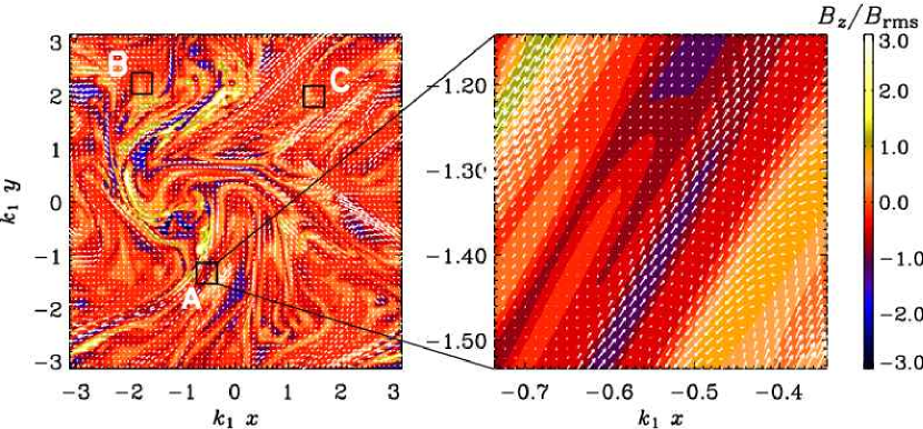
Figure 5.5: Snapshot of the magnetic field for $P_{\rm m}=50$, shown in a cross-section through the middle of the computational domain at a time when the field is in a saturated state. The data correspond to the spectra shown in Fig. 5.2. The field component perpendicular to the plane of the figure is shown color coded (or in shades of gray) with black corresponding to field pointing into the plane, and white to field pointing out of the plane. The field in the plane of the figure is shown with vectors whose length is proportional to the field strength. The right hand side shows an enlargement of the sub-domain A marked on the left hand side. Note the folded structures in sub-domain A.

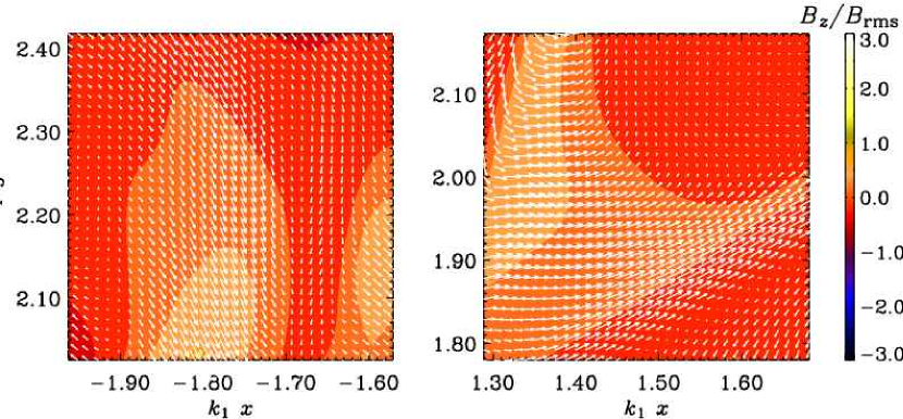
Figure 5.6: Magnetic field in sub-domains B and C that were indicated on the left hand side of Fig. 5.5. Note the lack of folded structures.

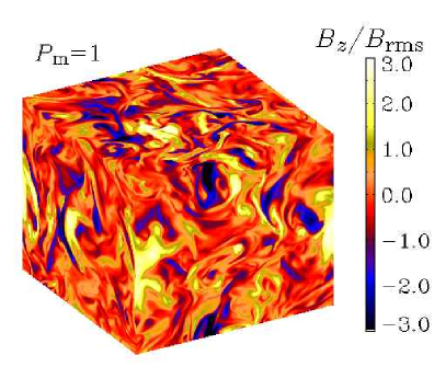
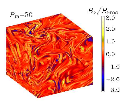
Figure 5.7: Comparison of $B_{z}$ (in shades of gray shown on the periphery of the box) for $P_{\rm m}=1$ (left) and $P_{\rm m}=50$ (right). The data shown here correspond to the spectra shown in Figs. 5.1 and 5.2, respectively. Note that the magnetic field for $P_{\rm m}=50$ is more intermittent in space and less space filling than for $P_{\rm m}=1$.

In Fig. 5.4 we show a visualization of the magnetic field vectors at those points where the magnetic field exceeds a certain field strength. The structures displayed represent a broad range of sizes even within one and the same structure: the thickness of the structures is often comparable to the resistive scale, their width is a bit larger (probably within the inertial range) and their length is comparable to the box size (subinertial range). Although large scales are involved in this simulations, we must distinguish them from the type of large scale magnetic fields seen in simulations with kinetic helicity that will be discussed in more detail in Section 8 and that are invoked to explain the solar cycle. Further, although the thickness of these structures is comparable to the resistive scale, we should keep in mind that these represent the rare structures with $|\bm{B}|>4B_{\rm rms}$, and are not volume filling.

At large magnetic Prandtl numbers the field shows folded structures that were discussed in detail by Schekochihin et al. [281]. An example of an arbitrarily chosen cross-section of a simulation with $P_{\rm m}=50$ is shown in Fig. 5.5, together with enlargements of different parts of the domain. The section A shows a region where the field is clearly folded; with the fairly straight field lines displaying rapid reversals transverse to its general direction. On the other hand there are also many other regions like B and C in the box, where the field is equally strong but is not in resistive scale folds. This illustrates that whereas there are folded structures, they need not be volume filling.

Folded structures are less prominent when $P_{\rm m}=1$. A comparison of the typical field structure for $P_{\rm m}=1$ and 50 is shown in Fig. 5.7, where we show color/gray scale representations of $B_{z}$ at an arbitrarily chosen moment during the saturated phase. The magnetic Reynolds number is $u_{\rm rms}/(\nu k_{\rm f})\approx 600$ and 4000 in the left and right hand panels, respectively, and the resolution is $512^{3}$ meshpoints in both cases.

For comparison with the analytic theory we plot in Fig. 5.8 the correlation function (5.9) of the magnetic field at saturation (and similarly for the velocity) for runs with $P_{\rm m}=1$ [254]. Similar autocorrelation functions have also been seen in simulations of convective dynamos [203]. It turns out that the velocity correlation length is $\sim 3$ (50% of the box size) while the magnetic field correlation length is $\sim 0.5$ (8% of the box size); see Fig. 5.8. (We recall that the box size is $2\pi$.) Clearly, the magnetic correlation length is much shorter than the velocity correlation length, but it is practically independent of Re ($=R_{\rm m}$) and certainly much longer than the resistive scale, $\sim 2\pi/k_{\rm d}\approx 0.04$ (0.7% if the box size). The fact that $w(r)$ in the saturated state is independent of the microscopic $R_{\rm m}$ agrees with the corresponding prediction of the closure model involving artificial nonlinear drifts [236, 257], discussed in Section 5.3.1.

Figure 5.8: Autocorrelation functions of magnetic field and velocity. Note that the autocorrelation functions are nearly independent of resolution and Reynolds number. The velocity correlation length is $\sim 3$ while the magnetic correlation length is $\sim 0.5$ (from Ref. [254]).

Figure 5.9: Saturation behavior of the spectral magnetic energy at wavenumbers $k=1$ (solid line) and $k=16$ (dashed line). The average forcing wavenumber is $k_{\rm f}=1.5$ and the resolution is $512^{3}$ meshpoints. Note the slow saturation behavior for $k=1$ (from Ref. [254]).

Figure 5.10: Evolution of characteristic wavenumbers. Note that the characteristic parallel wavenumber of the field, $k_{\parallel}$, becomes comparable with the scale of the box, while the so-called rms wavenumber, $k_{\rm rms}$, drops by almost a factor of two as saturation sets in. Here, $k_{\parallel}^{2}=\langle|\bm{B}\cdot\bm{\nabla}\bm{B}|^{2}\rangle/\langle\bm{B}^{4}\rangle$ and $k_{\rm rms}^{2}=\langle|\bm{\nabla}\bm{B}|^{2}\rangle/\langle\bm{B}^{2}\rangle$, where angular brackets denote volume averages. (The wavenumbers $k_{\bm{B}\times\bm{J}}$ and $k_{\bm{B}\cdot\bm{J}}$ are defined similarly to $k_{\parallel}$, but with $\bm{B}\times\bm{J}$ and $\bm{B}\cdot\bm{J}$, respectively, and follow a trend similar to that of $k_{\rm rms}$.) The rms wavenumber of the flow, $k_{\lambda}$, is proportional to the inverse Taylor microscale and decreases only slightly during saturation. Courtesy A. A. Schekochihin [281].

In contrast to large scale dynamos with helicity, which are now generally believed to have a resistively limited saturation phase in closed or periodic domains, the situation is less clear for nonhelical small scale dynamos; see Section 5.3.2 and Refs [245, 281]. The simulation results shown in Fig. 5.9 seem compatible with a slow saturation behavior for some intermediate time span ($80<u_{\rm rms}k_{\rm f}t<200$), but not at later times ($u_{\rm rms}k_{\rm f}t>200$).

As the small scale dynamo saturates, various magnetic length scales in the simulation increase quite sharply–some of them almost by a factor of two. For example, in convective dynamo simulations of a layer of depth $d$ the magnetic Taylor microscale, $\sqrt{5\langle\bm{B}^{2}\rangle/\langle\bm{J}^{2}\rangle}$, increased from $0.04d$ to $0.07d$ during saturation (see Fig. 4b of Ref. [203]). This increase of the characteristic length scale is in qualitative agreement with the analytic theory of the nonlinear saturation of the small scale dynamo (Section 5.3). In particular, during the kinematic stage these length scales remain unchanged. This can be seen from Fig. 5.10, where we show the evolution of various wavenumbers in a simulation of Schekochihin et al. [281]. The approximate constancy of the characteristic wavenumbers during the kinematic stage illustrates that the simple-minded picture of the evolution of single structures (Section 5.1) is different from the collective effect for an ensemble of many structures that are constantly newly generated and disappearing. We also note that in the saturated state the characteristic wavenumbers are approximately unchanged, suggesting that in the nonlinear regime there is no slow saturation phase (unlike the helical case that will be discussed later). During saturation, the drop of various characteristic wavenumbers is comparable to the increase of the Taylor microscale seen in the convective dynamo simulations [203].

5.5 Comments on the Batchelor mechanism and $P_{\rm m}$ dependence

In an early attempt to understand the possibility of small scale dynamo action, Batchelor [231] appealed to the formal analogy between the induction equation and the vorticity equation,

$${\mathrm{D}\bm{W}\over\mathrm{D}t} = \bm{W}\cdot\bm{\nabla}\bm{U}+\nu\nabla^{2}\bm{W},$$ (5.20)

$${\mathrm{D}\bm{B}\over\mathrm{D}t} = \bm{B}\cdot\bm{\nabla}\bm{U}+\eta\nabla^{2}\bm{B}.$$ (5.21)

These equations imply the following evolution equations for enstrophy and magnetic energy,

$${\textstyle{1\over 2}}{\mathrm{d}\langle\bm{W}^{2}\rangle\over\mathrm{d}t} = W_{i}W_{j}s_{ij}-\nu\langle(\bm{\nabla}\times\bm{W})^{2}\rangle,$$ (5.22)

$${\textstyle{1\over 2}}{\mathrm{d}\langle\bm{B}^{2}\rangle\over\mathrm{d}t} = B_{i}B_{j}s_{ij}-\eta\langle(\bm{\nabla}\times\bm{B})^{2}\rangle,$$ (5.23)

where $s_{ij}={\textstyle{1\over 2}}(u_{i,j}+u_{j,i})$ is the rate of strain tensor. Assuming that the rate of enstrophy dissipation, $\nu\langle(\bm{\nabla}\times\bm{W})^{2}\rangle$, is approximately balanced by the rate of enstrophy production, $W_{i}W_{j}s_{ij}$, and that this rate is similar to the rate of magnetic energy production, Batchelor argued that magnetic energy would grow in time provided $\eta<\nu$, i.e.

$$P_{\rm m}\equiv\nu/\eta>1.$$ (5.24)

By now there have been several numerical investigations of small scale dynamos that operate in a regime where the magnetic Prandtl number is less than unity. However, it is still not clear whether there exists a critical value of $P_{\rm m}$ below which no dynamo action is possible [282], whether the critical magnetic Reynolds number becomes independent of $P_{\rm m}$ for small enough values [244, 283], or whether, as $P_{\rm m}$ decreases, there continues to be a rise of the critical magnetic Reynolds number [254].

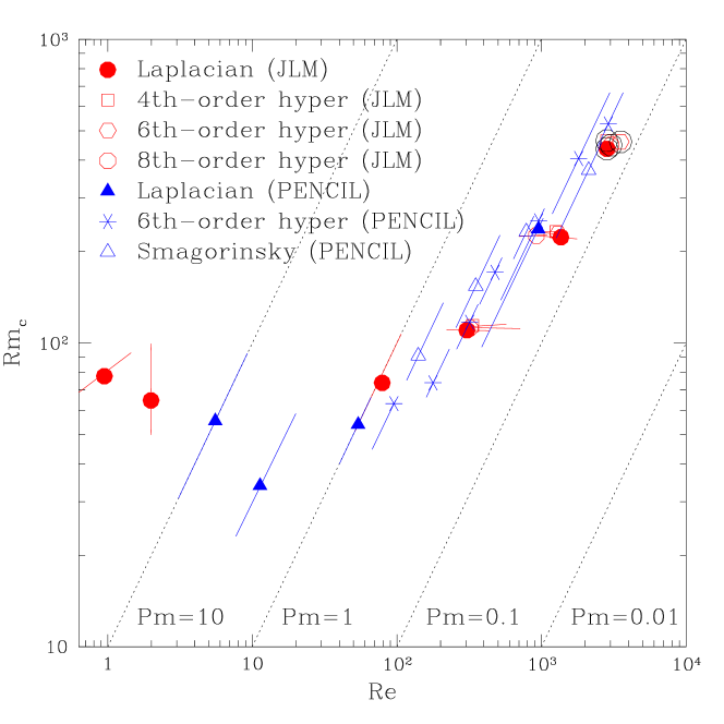
Figure 5.11: Dependence of $R_{\rm crit}$ on Re. “JLM” refers to simulations done with the incompressible spectral code written by J. L. Maron: runs with Laplacian viscosity, 4th-, 6th-, and 8th-order hyperviscosity (resolutions $64^{3}$ to $256^{3}$). In this set of simulations, hyperviscous runs were done at the same values of $\eta$ as the Laplacian runs, so the difference between the results for these runs is nearly imperceptible. “PENCIL” refers to weakly compressible simulations done with the Pencil Code: runs with Laplacian viscosity, 6th-order hyperviscosity, and Smagorinsky large-eddy viscosity (resolutions $64^{3}$ to $512^{3}$). Courtesy A. A. Schekochihin [273].

Comparing with Batchelor’s argument, the main reason why his argument may not apply is that, again, the $\bm{W}$ and $\bm{B}$ fields are in general not identical, and they do in general show quite different statistics [201, 203]. (Also $\bm{W}$ obeys a nonlinear equation, while $\bm{B}$ obeys a linear equation for a given $\bm{U}$.) Establishing the asymptotic dependence of $R_{\rm crit}$ on $P_{\rm m}$ is important because, even though the computing power will increase, it will still not be possible to simulate realistic values of $P_{\rm m}$ in the foreseeable future. Schekochihin et al. [273] have compared the results from two independent codes and show that there is as yet no evidence for an asymptotic independence of $R_{\rm crit}$ on $P_{\rm m}$; see Fig. 5.11.

We note that Fig. 5.11 compares not only the results of two different codes, but at the same time the results of an incompressible calculation with one of the weakly compressible equations (Mach number about 0.1). No significant difference is seen between the two simulations. However, when the flow becomes transonic (Mach number about 1), the critical magnetic Reynolds number increases by about a factor of 2; see Ref. [284] for results with $P_{\rm m}=1$ and 5.

Finally, we mention one property where the $\bm{W}$ and $\bm{B}$ fields do seem to show some similarity. For a $k^{-5/3}$ spectrum of kinetic energy the enstrophy spectrum is proportional to $k^{1/3}$, so one may expect a similar spectrum for the magnetic energy in the wavenumber range where feedback from the Lorentz force can be neglected. Such results have indeed been reported in the context of convection [203] and forced turbulence [254] during the kinematic stage. For forced turbulence, a $k^{1/3}$ spectrum has only been seen in the range $k_{1}<k<k_{\rm p}$, where $k_{\rm p}\approx k_{\rm f}R_{\rm crit}^{1/2}$ is the wavenumber where the magnetic energy spectrum peaks; see Fig. 5.3 and Section 5.4. We should emphasize, however, that it is not clear that this result is really a consequence of the (imperfect) analogy between $\bm{W}$ and $\bm{B}$.

5.6 Small and large scale dynamos: a unified treatment

We have so far discussed the case of small scale dynamos where the generated field has correlation lengths of order or smaller than the forcing scale of the flow. In the next section and thereafter we will discuss large scale or mean field dynamos. The large and small scale dynamo problems are usually treated separately. However this separation is often artificial; there is no abrupt transition from the field correlated on scales smaller than $L$ and that correlated on larger scales. If we consider both large and small scale fields to be random fields, it turns out that the equations for the magnetic correlation functions, which involve now both longitudinal and helical parts, are already sufficiently general to incorporate both small and large scale dynamos. They provide us with a paradigm to study the dynamics in a unified fashion, which could be particularly useful for studying the inverse cascade of magnetic fields to scales larger than $L$. We elaborate below.

We add a helical piece to the two point correlation of the velocity field for the Kazantsev-Kraichnan flow, so we have

$$T_{ij}(r)=\left(\delta_{ij}-{r_{i}r_{j}\over r^{2}}\right)\,T_{N}(r)+{r_{i}r_{j}\over r^{2}}\,T_{L}(r)+\epsilon_{ijk}r_{k}\,F(r),$$ (5.25)

where $F(r)$ represents the helical part of the velocity correlations. At $r=0$, we have

$$-2F(0)=-{\textstyle{1\over 3}}\int_{0}^{t}\langle\bm{v}(t)\cdot\bm{\nabla}\times\bm{v}(t^{\prime})\rangle\;\mathrm{d}t^{\prime},$$ (5.26)

indicating that $F(r)$ is related to the kinetic helicity of the flow.

Consider a system of size $S\gg L$, for which the mean field averaged over any scale is zero. Of course, the concept of a large scale field still makes sense, as the correlations between field components separated at scales $r\gg L$, can in principle be non-zero.

Since the flow can be helical, we need to allow the magnetic field to also have helical correlations. So, the equal-time, two point correlation of the magnetic field, $M_{ij}(r,t)$, is now given by

$$M_{ij}=\left(\delta_{ij}-{r_{i}r_{j}\over r^{2}}\right)\,M_{\rm N}+{r_{i}r_{j}\over r^{2}}\,M_{\rm L}+\epsilon_{ijk}r_{k}\,C,$$ (5.27)

where $C(r,t)$ represents the contribution from current helicity to the two-point correlation.

The Kazantsev equation can now be generalized to describe the evolution of both $M_{\rm L}$ and $C$ [236, 257, 285, 286] (see Appendix A). We get

$${\partial M_{\rm L}\over\partial t}={2\over r^{4}}{\partial\over\partial r}\left[r^{4}\eta_{\rm T}{\partial M_{\rm L}\over\partial r}\right]+GM_{\rm L}+4\alpha C,$$ (5.28)

$${\partial H\over\partial t}=-2\eta_{\rm T}C+\alpha M_{\rm L},\quad C=-\left(H^{\prime\prime}+{4H^{\prime}\over r}\right),$$ (5.29)

where $M_{\rm L}=M_{\rm L}(r,t)$ and $C=C(r,t)$, while $\alpha=\alpha(r)$ and $\eta_{\rm T}=\eta_{\rm T}(r)$, and we have defined the magnetic helicity correlation function $H(r,t)$. Note that $H(0,t)={1\over 6}\overline{\bm{A}\cdot\bm{B}}$, whereas $C(0,t)={1\over 6}\overline{\bm{J}\cdot\bm{B}}$. Also,

$$\alpha(r)=-2[F(0)-F(r)],$$ (5.30)

and so represents the effect of the helicity in the velocity field on the magnetic field. [We will see later in Section 8.10 that $\alpha(r\to\infty)$ is what is traditionally called the $\alpha$ effect]. This new term has some surprising consequences.

Suppose $\alpha_{0}=-2F(0)\neq 0$. Then one can see from Eqs. (5.28) and (5.29), that new “regenerating” terms arise at $r\gg L$, or for scales much larger than the correlation scales of the flow, due to the $\alpha$ effect. These are in the form $\dot{M}_{\rm L}=....+4\alpha_{0}C$ and $\dot{H}=...+\alpha_{0}M$, which couple $M_{\rm L}$ and $C$ and lead to the growth of large scale correlations. There is also decay of the correlations for $r\gg L$ due to diffusion with an effective diffusion coefficient, $\eta_{\rm T0}=\eta+T_{L}(0)$. From dimensional analysis, the effective growth rate is $\Gamma_{R}\sim\alpha_{0}/R-\eta_{\rm T0}/R^{2}$ for correlations on scale $\sim R$. This is exactly as in the large scale $\alpha^{2}$ dynamo to be discussed in the next section. This also picks out a special scale $R_{0}\sim\eta_{\rm T0}/\alpha_{0}$ for a stationary state (see below). Further, as the small scale dynamo, is simultaneously leading to a growth of $M_{\rm L}$ at $r<L$, the growth of large scale correlations can be seeded by the tail of the small scale dynamo eigenfunction at $r>L$. Indeed, as advertised, both the small and large scale dynamos operate simultaneously when $\alpha_{0}\neq 0$, and can be studied simply by solving for a single function $M_{\rm L}(r,t)$.

The coupled time evolution of $H$ and $M_{\rm L}$ for a non-zero $\alpha_{0}$ requires numerical solution, which we discuss later in Section 8.10. But interesting analytical insight into the system can be obtained for the marginal, quasi-stationary mode, with $\dot{M_{\rm L}}\approx 0$, $\dot{H}\approx 0$. Note that for $\eta\neq 0$, we will find that the above system of equations always evolves the correlation function at the resistive time scale. But for time scales much shorter than this, one can examine quasi-stationary states. For $\dot{H}\approx 0$, we get from Eq. (5.29) $C\approx[\alpha(r)/2\eta_{\rm T}(r)]M$. Substituting this into Eq. (5.28) and defining once again $\Psi=r^{2}\sqrt{\eta_{\rm T}}M_{\rm L}$, we get

$$-\eta_{\rm T}{d^{2}\Psi\over dr^{2}}+\Psi\left[U_{0}-{\alpha^{2}(r)\over\eta_{\rm T}(r)}\right]=0,$$ (5.31)

where $U_{0}$ is the potential defined earlier in Eq. (5.8). We see that the problem of determining the magnetic field correlations for the quasi-stationary mode once again becomes the problem of determining the zero-energy eigenstate in a modified potential, $U=U_{0}-\alpha^{2}/\eta_{\rm T}$. (Note that the $U$ in this subsection is not to be confused with velocity in other sections.) The addition to $U_{0}$, due to the helical correlations, is always negative definite. Therefore, helical correlations tend to make bound states easier to obtain. When $F(0)=0$, and there is no net $\alpha$ effect, the addition to $U_{0}$ vanishes at $r\gg L$, and $U\to 2\eta_{T}/r^{2}$ at large $r$, as before. The critical magnetic Reynolds number, for the stationary state, will however be smaller than when $F(r)\equiv 0$, because of the negative definite addition to $U_{0}$ (see also Ref. [287]).

Figure 5.12: Schematic illustration of the potential $U(r)$ for the marginal mode in helical turbulence. A non-zero $\alpha_{0}$ allows the tunneling of the zero-energy state to produce large scale correlations.

When $\alpha_{0}=-2F(0)\neq 0$, a remarkable change occurs in the potential. At $r\gg L$, where the turbulence velocity correlations vanish, we have $U(r)=2\eta_{\rm T0}/r^{2}-\alpha_{0}^{2}/\eta_{\rm T0}$. So the potential $U$ tends to a negative definite constant value of $-\alpha_{0}^{2}/\eta_{\rm T0}$ at large $r$ (and the effective mass changes, $1/2\eta_{\rm T}\to 1/2\eta_{\rm T0}$, which is independent of $r$.) So there are strictly no bound states, with zero energy/growth rate, for which the correlations vanish at infinity. We have schematically illustrated the resulting potential $U$ in Fig. 5.12, which is a modification of Fig. 8.4 of Zeldovich et al. [222]. In fact, for a non-zero $\alpha_{0}$, $U$ corresponds to a potential which allows tunneling (of the bound state) in the corresponding quantum mechanical problem. It implies that the correlations are necessarily non-zero at large $r>L$. The analytical solution to (5.31) at large $r\gg L$, is easily obtained. We have for $r\gg L$, $M_{\rm L}(r)={\bar{M}}_{\rm L}(r)\propto r^{-3/2}J_{\pm 3/2}(\mu r)$, where $\mu=\alpha_{0}/\eta_{\rm T0}=R_{0}^{-1}$. This corresponds to

$$w(r)={\bar{w}}(r)=\mu r^{-1}[C_{1}\sin\mu r+C_{2}\cos\mu r];\quad r\gg L,$$ (5.32)

where $C_{1},C_{2}$ are arbitrary constants. Clearly for a non-zero $\alpha_{0}$, the correlations in the steady state at large $r$, are like ‘free-particle’ states, extending to infinity! In fact this correlation function is also the one which one obtains if we demand the random field to be force free with $\bm{\nabla}\times\bm{B}=\mu\bm{B}$. We see therefore that having helicity in the flow opens up the possibility of generating large scale fields of scales much larger than that of the turbulent flow. This is the feature we will elaborate on more in the following sections.

5.7 Comments on anisotropy and nonlocality in MHD turbulence

The usual approach to MHD turbulence is to proceed analogously to hydrodynamic turbulence. Note that in hydrodynamic turbulence, one usually makes the assumption that the velocity field is statistically isotropic and homogeneous, and that the nonlinear interactions in wavenumber space are local. There is also a unique timescale associated with the nonlinear interactions, the eddy turnover time, $\tau_{k}=(kv_{k})^{-1}$, where $v_{k}=[2kE(k)]^{1/2}$ is the turbulent velocity at wavenumber $k$ and $E(k)$ is the 1-D kinetic energy spectrum. Demanding that in the ‘inertial range’ the energy transfer flux, $\epsilon=v_{k}^{2}/\tau_{k}$, is a constant, independent of scale, we have $v_{k}\propto k^{-1/3}$ and therefore the Kolmogorov spectrum $E(k)=C\epsilon^{2/3}k^{-5/3}$ for hydrodynamic turbulence.

There is a crucial difference in the presence of magnetic fields. A uniform velocity field simply advects the eddies and leaves the physical system unchanged (Galilean invariance). But a uniform (or large scale) magnetic field $\overline{\bm{B}}$, cannot be transformed away. Its presence supports propagation of hydromagnetic waves (Alfvén waves), and introduces a nonlocal coupling between small and large scales. Since these waves propagate along $\overline{\bm{B}}$ at the Alfvén speed $V_{\rm A}=\overline{B}/\sqrt{4\pi\rho}$, they introduce one more time scale, the Alfvén crossing time $\tau_{\rm A}(k)=(kV_{\rm A})^{-1}$, which can play a role in determining the turbulence properties. Furthermore, $\overline{\bm{B}}$ introduces a locally preferred direction, and the turbulence can in principle be anisotropic.

The work of Iroshnikov [288] and Kraichnan [289] (IK) emphasized the importance of the Alfvén crossing time $\tau_{\rm A}(k)$. Since the influential paper by Goldreich and Sridhar [26] it has become clear that anisotropy will also play a crucial role in MHD turbulence. We briefly discuss these ideas, before drawing comparisons with the MHD turbulence resulting from dynamo action. We focus on incompressible motions, split the magnetic field as $\bm{B}=\overline{\bm{B}}+\bm{b}$, and write the MHD equations in a more symmetric form, in terms of Elsasser fields $\bm{z}_{\pm}=\bm{u}\pm\bm{b}/\sqrt{4\pi\rho}$. We have, defining $\bm{V}_{\rm A}=\overline{\bm{B}}/\sqrt{4\pi\rho}$ as a vector,

$$\frac{\partial\bm{z}_{\pm}}{\partial t}\mp\bm{V}_{\rm A}\cdot\bm{\nabla}\bm{z}_{\pm}=-\bm{z}_{\mp}\cdot\bm{\nabla}\bm{z}_{\pm}-\bm{\nabla}\Pi+\nu\bm{\nabla}^{2}\bm{z}_{\pm}.$$ (5.33)

Here $\Pi=p/\rho+B^{2}/8\pi\rho$ acts to enforce $\bm{\nabla}\cdot\bm{z}_{\pm}=0$ and we have assumed for simplicity $\nu=\eta$.

Assuming either $\bm{z}_{+}=0$ or $\bm{z}_{-}=0$ gives exact solutions of the ideal MHD equations. The solution with $\bm{z}_{-}=0$ represents the Elsasser field $\bm{z}_{+}$ propagating non-dispersively in the direction of the mean field. A wave packet with $\bm{z}_{+}=0$, represents $\bm{z}_{-}$ propagating in the direction opposite to the mean field direction. Nonlinear interactions occur only if there is an overlap of both type of fluctuations, $\bm{z}_{\pm}$. This led Kraichnan [289] to suggest that energy transfer in MHD turbulence results from “collisions” between wave packets moving in opposite directions along the mean field. One can show from Eq. (5.33) that such collisions conserve the individual energies $\bm{z}_{\pm}^{2}$ of the oppositely traveling wave packets when $\nu=0$. Of course the total energy is also conserved under ideal MHD. These two conservation laws are equivalent to the conservation of the total energy and the cross helicity $H_{\rm cross}={\textstyle{1\over 2}}\int\bm{u}\cdot\bm{b}\,\mathrm{d}^{3}x={1\over 8}\int(\bm{z}_{+}^{2}-\bm{z}_{-}^{2})\,\mathrm{d}^{3}x$.

Suppose one assumes that equal amounts of $\bm{z}_{+}$ and $\bm{z}_{-}$ energies are present, and nonlinear interactions are due to oppositely directed wave packets. Such a collision occurs over the Alfvén crossing time of $1/(k_{\parallel}V_{\rm A})$, where $1/k_{\parallel}$ is the extent of the wave packet along $\overline{\bm{B}}$. The magnitude of the nonlinear interaction term $|\bm{z}_{\mp}\cdot\bm{\nabla}\bm{z}_{\pm}|\sim k_{\perp}z_{k_{\perp}}^{2}$, where $z_{k_{\perp}}$ is the magnitude of either Elsasser variable at wavenumber $k_{\perp}$, and $1/k_{\perp}$ is the extent of the wave packet transverse to $\overline{\bm{B}}$. (Here we have implicitly assumed that the component of $\bm{z}_{\mp}$ perpendicular to $\overline{\bm{B}}$ dominates over the parallel one, or that shear Alfvén waves dominate pseudo Alfvén waves [26, 290]). Due to the nonlinear term, the collision will then induce a fractional change $\chi$ in $\bm{z}_{\pm}$, given by

$$\chi\sim\frac{\delta z_{k_{\perp}}}{z_{k_{\perp}}}\sim\frac{k_{\perp}z_{k_{\perp}}}{k_{\parallel}V_{\rm A}}.$$ (5.34)

When $\chi\ll 1$ we are in the regime of weak turbulence. In this case, each collision results in a small random change in the wave packet. Since these changes add randomly, of order $N\sim 1/\chi^{2}\gg 1$ collisions are required for an order unity fractional change. This implies a time scale for the cascade of energy to a smaller scale of $\tau_{\rm cas}\sim\chi^{-2}(1/k_{\parallel}V_{\rm A})\sim(k_{\parallel}V_{\rm A})/(k_{\perp}z_{k_{\perp}})^{2}$.

Let us assume, naively following IK, that turbulence is isotropic, and take $z_{k_{\perp}}=z_{k}$, with wave packets having the same parallel and perpendicular scales, i.e. we put $k_{\parallel}=k_{\perp}=k$ in the above $\tau_{\rm cas}$. We demand that, far away from the injection or dissipative scales, the energy transfer flux, $\epsilon=z_{k}^{2}/\tau_{\rm cas}=z_{k}^{4}k/V_{\rm A}$, is a constant, independent of scale, we get $z_{k}\sim(\epsilon V_{\rm A}/k)^{1/4}$. Noting that the 1-D energy spectrum $E(k)\sim z_{k}^{2}/k$, we get the IK spectrum $E(k)\sim(\epsilon V_{\rm A})^{1/2}k^{-3/2}$. At best, the assumption of isotropy may be of use if the large scale field is itself randomly distributed in direction.

Also implicit in the above analysis is the importance of interactions which couple 3 waves. For weak turbulence these contribute to energy transfer only if the 3 waves satisfy the closure relations: $\omega_{1}+\omega_{2}=\omega_{3}$ and $\bm{k}_{1}+\bm{k}_{2}=\bm{k}_{3}$. Since $\omega=V_{\rm A}|k_{\parallel}|$, and the 3-mode coupling vanishes unless waves 1 and 2 propagate in opposite directions, the closure relations imply that either $k_{1\parallel}$ or $k_{2\parallel}$ must vanish, and the other parallel component equals $k_{3\parallel}$. So, for weak turbulence, 3-wave interaction do not cascade energy along $k_{\parallel}$.

Now suppose we do not make the assumption of isotropy, and keep $k_{\parallel}$ constant in working out the energy flux $\epsilon=z_{k_{\perp}}^{2}/\tau_{\rm cas}$. Then, setting $\epsilon$ to a constant in the inertial range gives $z_{k_{\perp}}\sim(\epsilon k_{\parallel}V_{\rm A}/k_{\perp}^{2})^{1/4}$. Defining the 1-D anisotropic spectrum by $k_{\perp}E(k_{\perp})=z_{k_{\perp}}^{2}$, we get

$$E(k_{\perp})=z_{k_{\perp}}^{2}/k_{\perp}\sim\frac{(\epsilon k_{\parallel}V_{\rm A})^{1/2}}{k_{\perp}^{2}}.$$ (5.35)

From the expression for $z_{k_{\perp}}$ we also see that the strength of nonlinear interactions is $\chi\propto k_{\perp}^{1/2}$. So, for small enough scales $\chi$ becomes of order unity and turbulence becomes strong.

Indeed strong MHD turbulence is the relevant one for most astrophysical applications, not only because of the above, but also because the stirring velocities and fields are comparable to $\overline{\bm{B}}$. Recall that in weak Alfvénic turbulence, where $\chi\ll 1$, the Alfvén time $\tau_{\rm A}=(k_{\parallel}V_{\rm A})^{-1}$ was small compared to the nonlinear interaction time $\tau_{\rm nl}=(k_{\perp}z_{k_{\perp}})^{-1}$. In fact we can write $\chi=\tau_{\rm A}/\tau_{\rm nl}$. GS argued that strong MHD turbulence exhibits what they refer to as a critical balance, whereby these 2 timescales become comparable, and $\chi\sim 1$. We already saw that if $\chi$ were small then at small enough scales it grows to order unity. On the other hand, were $\chi\gg 1$, for example because $k_{\parallel}<k_{c}=k_{\perp}z_{k_{\perp}}/V_{\rm A}$, then as the wave packets go through each other over a distance $1/k_{c}<1/k_{\parallel}$, strong distortions are already introduced, thereby creating structures with $k_{\parallel}=k_{c}$ (see the pictorial illustration in Ref. [291]). As a result, $\chi$ is driven to unity. It seems plausible therefore that something like critical balance is a stable fixed point of the system.

Critical balance implies that the cascade time is comparable to the other time scales, $\tau_{\rm cas}\sim\tau_{\rm A}\sim\tau_{\rm nl}$. Assuming again a scale independent energy flux $\epsilon=z_{k_{\perp}}^{2}/\tau_{\rm cas}=z_{k_{\perp}}^{3}k_{\perp}$, we get the GS relations

$$z_{k_{\perp}}\sim V_{\rm A}(k_{\perp}L)^{1/3},\quad k_{\parallel}\sim k_{\perp}^{2/3}L^{-1/3}.$$ (5.36)

Here we have used the estimate $\epsilon=V_{\rm A}^{3}/L$, assuming that the perturbed velocities are of order $V_{\rm A}$, and the scale of stirring is $L$. These scalings imply that the parallel and perpendicular sizes of eddies are correlated, with the eddies becoming highly elongated at small scales, even if they were isotropic at the forcing scale. We can define the three-dimensional spectrum $\bar{E}(k_{\perp},k_{\parallel})$ using $\int\bar{E}\,\mathrm{d}^{3}k=\sum z_{k_{\perp}}^{2}$. Since $k_{\parallel}\sim k_{\perp}^{2/3}L^{-1/3}$, this spectrum can be written as $\bar{E}(k_{\perp},k_{\parallel})=Af(k_{\parallel}L^{1/3}/k_{\perp}^{2/3})$, where $f(x)$ is a positive, symmetric function of $x$, which is of order 1 for $x<1$ and is negligible for $|x|\gg 1$. We can fix the dependencies in the normalization constant $A$ by changing variables in the integral over $\mathrm{d}k_{\parallel}$ to $x=k_{\parallel}L^{1/3}/k_{\perp}^{2/3}$, and using the definition of $\bar{E}$. We get the anisotropic Kolmogorov spectrum [26]

$$\bar{E}(k_{\perp},k_{\parallel})\sim\frac{V_{\rm A}^{2}}{k_{\perp}^{10/3}L^{1/3}}f\left(\frac{k_{\parallel}L^{1/3}}{k_{\perp}^{2/3}}\right).$$ (5.37)

GS also derived a kinetic equation where this spectrum arises as a stationary solution. For some succinct reviews see also [291, 292].

We note that in all the above discussions, the large scale field is assumed to be given or imposed. In this case, we see that it will introduce anisotropy at all scales, implying spectral nonlocality to all smaller scales. The full extent of the possible departures from isotropy and locality in wavenumber space, when the large scale field is generated during dynamo action, is yet to be clarified. It remains therefore to be seen whether in isotropically forced turbulence (without imposed field and just the dynamo-generated small scale field) the field averaged over any local sub-domain really introduces nonlocality on all smaller scales within this domain. If so, one would expect the spectrum of the hydromagnetic turbulence with imposed field to be similar to the deeper parts of the spectrum in hydromagnetic turbulence without imposed field. This does not seem to be the case, because in the latter case the spectral magnetic energy is found to be in super-equipartition (see Fig. 5.3). This behavior is not seen in simulations with imposed field where the spectrum of magnetic energy is rather in sub-equipartition if the field is strong.

The effect of anisotropy due to the mean field on the turbulent transport coefficients has been considered in a number of papers, but no explicit connection with the Goldreich–Sridhar theory has yet been made. The anisotropic cascade is potentially quite important for a proper understanding of turbulent magnetic diffusion. Further in discussing MHD turbulence, most of the semi-analytical works set magnetic helicity to zero. Inclusion of helicity is important to make connection with the large scale dynamo generated MHD turbulence.

6 Large scale turbulent dynamos

As the simulation results of Section 5.4 and the unified treatment in Section 5.6 have shown, the distinction between small and large scale dynamos is somewhat artificial. The so-called small scale dynamo may well generate magnetic field structures extending all the way across the computational domain; see Fig. 5.4. On the other hand, the overall orientation of these structures is still random. This is in contrast to the spatio-temporal coherence displayed by the sun’s magnetic field, where the overall orientation of flux tubes at a certain location in space and time follows a regular rule and is not random. Dynamo mechanisms that explain this will be referred to as large scale dynamos. Here the geometry of the domain and the presence of boundaries and shear are important.

In this section we discuss the basic theory of large scale dynamos in terms of the alpha effect and discuss simple models. A discussion of large scale dynamos in terms of the inverse cascade is presented in the next section.

6.1 Phenomenological considerations

Important insights into the operation of the solar dynamo have come from close inspection of magnetic fields on the solar surface [210]. One important ingredient is differential rotation. At the equator the sun is rotating about 30% faster than at the poles. This means that any poloidal field will be sheared out and toroidal field aligned with the direction of the shear will be generated. Mathematically, this is described by the stretching term in the induction equation; see Eq. (3.19), i.e.

$${\mathrm{d}\bm{B}_{\rm tor}\over\mathrm{d}t}=\bm{B}_{\rm pol}\cdot\bm{\nabla}\bm{U}_{\rm tor}+...\,.$$ (6.1)

This term describes the generation of magnetic field $\bm{B}_{\rm tor}$ in the direction of the flow $\bm{U}_{\rm tor}$ from a cross-stream poloidal magnetic field $\bm{B}_{\rm pol}$. To an order of magnitude, the amount of toroidal field generation from a $100\,{\rm G}$ poloidal field in a time interval $\Delta t=10^{8}\,{\rm s}=3\,{\rm yr}$ is

$$\Delta\bm{B}_{\rm tor}=\bm{B}_{\rm pol}\;\Delta\Omega_{\odot}\Delta t\approx 100\,{\rm G}\times 10^{-6}\times 10^{8}=10^{4}\,{\rm G},$$ (6.2)

where we have used $\Omega_{\odot}=3\times 10^{-6}\,{\rm s}^{-1}$ for the solar angular velocity, and $\Delta\Omega_{\odot}/\Omega_{\odot}=0.3$ for the relative latitudinal differential rotation. So, a $10\,{\rm kG}$ toroidal field can be regenerated completely from a $100\,{\rm G}$ poloidal field in about 3 years. However, in the bulk and the upper parts of the solar convection zone the poloidal fields are weaker ($3$-$10\,{\rm G}$), which would yield toroidal fields on the order of $300$-$1000\,{\rm G}$. This would be far too weak a field if it was to rise coherently all the way from the bottom of the convection zone, which is still the standard picture. However, if the field of bipolar regions is produced locally in the upper parts of the convection zone, as recently supposed in Ref. [55], a $300\,{\rm G}$ field might well be sufficient. The $2\,{\rm kG}$ fields in sunspots could then be the result of local compression by an ambient flow.

On the other hand, according to the standard picture (see Section 2.1.1) the $100\,{\rm kG}$ field, necessary to give the right tilt of emerging flux tubes, can perhaps be explained as the result of stretching of more localized $\sim 1\,{\rm kG}$ field patches that stay coherent over a time span of about $3\,{\rm yr}$.

In the bulk of the solar convection zone the turnover time, $\tau_{\rm turnover}=u_{\rm rms}/H_{p}$ (where $H_{p}$ is the pressure scale height) is only about 10 days. In order that a toroidal field can be generated, a mean poloidal field needs to be maintained and, in the case of the sun and other stars with cyclic field reversals, the poloidal field itself needs to change direction every 11 years.

Magnetic flux frequently emerges at the solar surface as bipolar regions. The magnetic field in sunspots is also often of bipolar nature. It was long recognized that such bipolar regions are tilted. This is now generally referred to as Joy’s law [37, 293]. The sense of average tilt is clockwise in the northern hemisphere and counter-clockwise in the southern. This tilt is consistent with the interpretation that a toroidal flux tube rises from deeper layers of the sun to upper layers where the density is less, so the tube evolves in an expanding flow field which, due to the Coriolis force, attains a clockwise swirl in the northern hemisphere and counter-clockwise swirl in the southern hemisphere; see Fig. 6.1.

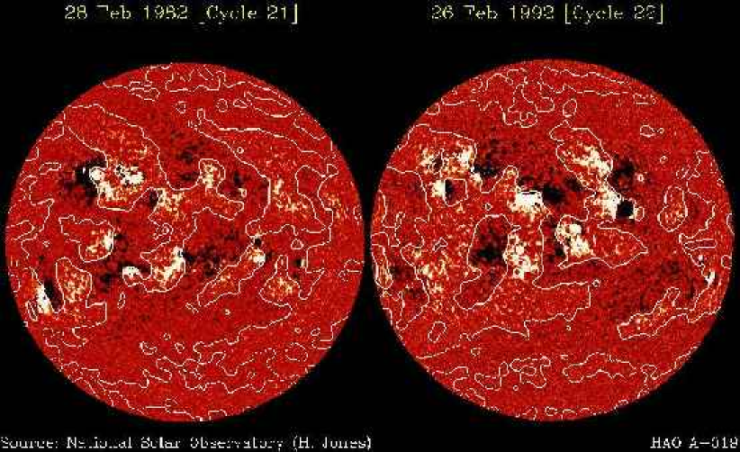
Figure 6.1: Solar magnetogram showing bipolar regions, their opposite orientation north and south of the equator, and the clockwise tilt in the northern hemisphere and the counter-clockwise tilt in the southern hemisphere. Note that the field orientation has reversed orientation at the next cycle (here after 10 years). Courtesy of the High Altitude Observatory.

Figure 6.2: Sketch of the Babcock-Leighton dynamo mechanism. As bipolar regions emerge near the surface, they get tilted in the clockwise sense in the northern hemisphere and counter-clockwise in the southern hemisphere. Beneath the surface this process leaves behind a poloidal field component that points here toward the north pole on either side of the equator. Once the remaining subsurface field gets sheared by the surface differential rotation, it points in the opposite direction as before, and the whole process starts again.

Observations suggest that once a tilted bipolar region has emerged at the solar surface, the field polarities nearer to the poles drift rapidly toward the poles, producing thereby new poloidal field [210, 294]. Underneath the surface, the field continues as before, but there it is also slightly tilted, although necessarily in the opposite sense (see Fig. 6.2). Because of differential rotation, the points nearest to the equator move faster, helping so to line up similarly oriented fields [295]. As is evident from Fig. 6.2, a toroidal field pointing east in the northern hemisphere and west in the southern will develop into a global northward pointing field above the surface.

6.2 Mean-field electrodynamics

Parker [209] first proposed the idea that the generation of a poloidal field, arising from the systematic effects of the Coriolis force (Fig. 6.3), could be described by a corresponding term in the induction equation,

$${\partial\overline{\bm{B}}_{\rm pol}\over\partial t}=\bm{\nabla}\times\left(\alpha\overline{\bm{B}}_{\rm tor}+...\right).$$ (6.3)

It is clear that such an equation can only be valid for averaged fields (denoted by overbars), because for the actual fields, the induced electromotive force (EMF) $\bm{U}\times\bm{B}$, would never have a component in the direction of $\bm{B}$. While being physically plausible, this approach only received general recognition and acceptance after Roberts and Stix [296] translated the work of Steenbeck, Krause, Rädler [297] into English. In those papers the theory for the $\alpha$ effect, as they called it, was developed and put on a mathematically rigorous basis. Furthermore, the $\alpha$ effect was also applied to spherical models of the solar cycle (with radial and latitudinal shear) [298] and the geodynamo (with uniform rotation) [299].

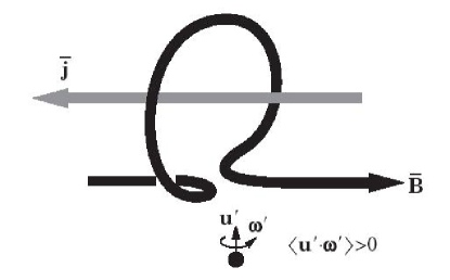
Figure 6.3: Production of positive writhe helicity by an uprising and expanding blob tilted in the clockwise direction by the Coriolis force in the southern hemisphere, producing a field-aligned current $\overline{\mbox{\boldmath$J$}}$ in the opposite direction to $\overline{\bm{B}}$. Courtesy of A. Yoshizawa [22].

In mean field theory one solves the Reynolds averaged equations, using either ensemble averages, toroidal averages or, in cases in cartesian geometry with periodic boundary conditions, two-dimensional (e.g. horizontal) averages. We thus consider the decomposition

$$\bm{U}=\overline{\mbox{\boldmath$U$}}+\bm{u},\quad\bm{B}=\overline{\bm{B}}+\bm{b}.$$ (6.4)

Here $\overline{\mbox{\boldmath$U$}}$ and $\overline{\bm{B}}$ are the mean velocity and magnetic fields, while $\bm{u}$ and $\bm{b}$ are their fluctuating parts. These averages satisfy the Reynolds rules,

$$\overline{\bm{U}_{1}+\bm{U}_{2}}=\overline{\mbox{\boldmath$U$}}_{1}+\overline{\mbox{\boldmath$U$}}_{2},\quad\overline{\overline{\mbox{\boldmath$U$}}}=\overline{\mbox{\boldmath$U$}},\quad\overline{\overline{\mbox{\boldmath$U$}}\bm{u}}=0,\quad\overline{\overline{\mbox{\boldmath$U$}}_{1}\;\overline{\mbox{\boldmath$U$}}_{2}}=\overline{\mbox{\boldmath$U$}}_{1}\;\overline{\mbox{\boldmath$U$}}_{2},$$ (6.5)

$$\overline{\partial\bm{U}/\partial t}=\partial\overline{\mbox{\boldmath$U$}}/\partial t,\quad\overline{\partial\bm{U}/\partial x_{i}}=\partial\overline{\mbox{\boldmath$U$}}/\partial x_{i}.$$ (6.6)

Some of these properties are not shared by several other averages; for gaussian filtering $\overline{\overline{\mbox{\boldmath$U$}}}\neq\overline{\mbox{\boldmath$U$}}$, and for spectral filtering $\overline{\overline{\mbox{\boldmath$U$}}\;\overline{\mbox{\boldmath$U$}}}\neq\overline{\mbox{\boldmath$U$}}\;\overline{\mbox{\boldmath$U$}}$, for example. Note that $\overline{\overline{\mbox{\boldmath$U$}}}=\overline{\mbox{\boldmath$U$}}$ implies that $\overline{\bm{u}}=0$.

Here a comment on scale separation is in order. The averaging procedure discussed above is valid even if there is hardly any scale separation, i.e. if the averaging length of the container is close to the eddy scale. One concern is that an $\alpha^{2}$ type large scale dynamo field (i.e. a mean field that is generated without shear; see below) may no longer be excited; see Section 9.4.1. But apart from this, the absence of scale separation does not impose any technical restrictions. Poor scale separation does however imply that the averages are not smooth in time and in the directions in which no averaging is performed. This, in turn, is reflected in the fact that turbulent transport coefficients estimated from simulations can be very noisy.

Scale separation does become an issue, however, if one wants to use averages for which the Reynolds rules are not obeyed. For example, if mean field theory is to model nonaxisymmetric features of stellar or galactic magnetic fields, one would like to define a mean field by averaging over small volumes. In order that the Reynolds rules remain then at least approximately valid, scale separation must be invoked.

In the remainder we assume that the Reynolds rules do apply. Averaging Eq. (3.11) yields then the mean field induction equation,

$${\partial\overline{\bm{B}}\over\partial t}=\bm{\nabla}\times\left(\overline{\mbox{\boldmath$U$}}\times\overline{\bm{B}}+\overline{\mbox{\boldmath${\mathcal{E}}$}}{}-\eta\overline{\mbox{\boldmath$J$}}\right),$$ (6.7)

where

$$\overline{\mbox{\boldmath${\mathcal{E}}$}}{}=\overline{\bm{u}\times\bm{b}}$$ (6.8)

is the mean EMF. Finding an expression for the correlator $\overline{\mbox{\boldmath${\mathcal{E}}$}}{}$ in terms of the mean fields is a standard closure problem which is at the heart of mean field theory. In the two-scale approach [148] one assumes that $\overline{\mbox{\boldmath${\mathcal{E}}$}}{}$ can be expanded in powers of the gradients of the mean magnetic field. This suggests the rather general expression

$${\cal E}_{i}=\alpha_{ij}(\hat{\bm{g}},\hat{\bm{\Omega}},\overline{\bm{B}},...)\overline{B}_{j}+\eta_{ijk}(\hat{\bm{g}},\hat{\bm{\Omega}},\overline{\bm{B}},...)\partial\overline{B}_{j}/\partial x_{k},$$ (6.9)

where the tensor components $\alpha_{ij}$ and $\eta_{ijk}$ are referred to as turbulent transport coefficients. They depend on the stratification, angular velocity, and mean magnetic field strength. The dots indicate that the transport coefficients may also depend on correlators involving the small scale magnetic field, for example the current helicity of the small scale field, as will be discussed in Section 9.3. We have also kept only the lowest large scale derivative of the mean field; higher derivative terms are expected to be smaller (cf. Section 7.2 in Moffatt [148]), although this may not be justified in certain cases [300].

The general subject has been reviewed in many text books [148, 301], but the importance of the small scale magnetic field (or rather the small scale current helicity) has only recently been appreciated [302, 303], even though the basic equations were developed much earlier [9, 304]. This aspect of the problem will be discussed in more detail in Section 8.7.

The general form of the expression for $\overline{\mbox{\boldmath${\mathcal{E}}$}}{}$ can be determined by rather general considerations [301]. For example, $\overline{\mbox{\boldmath${\mathcal{E}}$}}{}$ is a polar vector and $\overline{\bm{B}}$ is an axial vector, so $\alpha_{ij}$ must be a pseudo-tensor. The simplest pseudo-tensor of rank two that can be constructed using the unit vectors $\hat{\bm{g}}$ (symbolic for radial density or turbulent velocity gradients) and $\hat{\bm{\Omega}}$ (angular velocity) is

$$\alpha_{ij}=\alpha_{1}\delta_{ij}\,\hat{\bm{g}}\cdot\hat{\bm{\Omega}}+\alpha_{2}\hat{g}_{i}\hat{\Omega}_{j}+\alpha_{3}\hat{g}_{j}\hat{\Omega}_{i}.$$ (6.10)

Note that the term $\hat{\bm{g}}\cdot\hat{\bm{\Omega}}=\cos\theta$ leads to the co-sinusoidal dependence of $\alpha$ on latitude, $\theta$, and a change of sign at the equator. Additional terms that are nonlinear in $\hat{\bm{g}}$ or $\hat{\bm{\Omega}}$ enter if the stratification is strong or if the body is rotating rapidly. Likewise, terms involving $\overline{\mbox{\boldmath$U$}}$, $\overline{\bm{B}}$ and $\bm{b}$ may appear if the turbulence becomes affected by strong flows or magnetic fields. In the following subsection we discuss various approaches to determining the turbulent transport coefficients.

One of the most important outcomes of this theory is a quantitative formula for the coefficient $\alpha_{1}$ in Eq. (6.10) by Krause [305],

$$\alpha_{1}\,\hat{\bm{g}}\cdot\hat{\bm{\Omega}}=-{\textstyle{16\over 15}}\tau_{\rm cor}^{2}u_{\rm rms}^{2}\bm{\Omega}\cdot\bm{\nabla}\ln(\rho u_{\rm rms}),$$ (6.11)

where $\tau_{\rm cor}$ is the correlation time, $u_{\rm rms}$ the root mean square velocity of the turbulence, and $\bm{\Omega}$ the angular velocity vector. The other coefficients are given by $\alpha_{2}=\alpha_{3}=-\alpha_{1}/4$. Throughout most of the solar convection zone, the product $\rho u_{\rm rms}$ decreases outward. Therefore, $\alpha>0$ throughout most of the northern hemisphere. In the southern hemisphere we have $\alpha<0$, and $\alpha$ varies with colatitude $\theta$ like $\cos\theta$. However, this formula also predicts that $\alpha$ reverses sign very near the bottom of the convection zone where $u_{\rm rms}\to 0$. This is caused by the relatively sharp drop of $u_{\rm rms}$ [306].

The basic form and sign of $\alpha$ is also borne out by simulations of stratified convection [307, 308]. One aspect that was first seen in simulations is the fact that in convection the vertical component of the $\alpha$ effect can have the opposite sign compared with the horizontal components [307, 308]. The same result has later been obtained in analytic calculations of the $\alpha$ effect in supernova-driven interstellar turbulence [309] and in first order smoothing approximation (FOSA) calculations [310].

6.3 Calculation of turbulent transport coefficients

Various techniques have been proposed for determining turbulent transport coefficients. Even in the kinematic regime, where the changes in the velocity field due to Lorentz forces are ignored, these techniques have some severe uncertainties. Nevertheless, the various techniques produce similar terms, although the so-called minimal $\tau$ approximation (MTA) does actually predict an extra time derivative of the electromotive force [8]. This will be discussed in full detail in Section 10. We only mention here that in MTA the triple correlations are not neglected, as they are in FOSA; see Section 6.3.1. Instead, the triple correlations are approximated by quadratic terms. This is similar in spirit to the usual $\tau$ approximation used in the Eddy Damped Quasi-Normal Markovian (EDQNM) closure approximation (see Section 7.2), where the irreducible part of quartic correlations are approximated by a relaxation term proportional to the triple correlations. Other approaches include direct simulations [307, 308, 311] (see Section 6.4), calculations based on random waves [148, 312, 313] or individual blobs [309, 314] (see Section B.2.1), or calculations based on the assumption of delta-correlated velocity fields [13, 235, 315] (Section B.2). A summary of the different approaches, their properties and limitations is given in Table LABEL:Tsum.

One of the most promising approaches is indeed MTA, because there is now some numerical evidence from turbulence simulations that MTA may be valid even when the fluctuations are large and the correlation time not very short; see Section 9.2, and Ref. [316]. This is of course beyond the applicability regime of FOSA. Early references to MTA include the papers of Vainshtein and Kitchatinov [317] and Kleeorin and collaborators [318, 319, 320], but since MTA is based on a closure hypothesis, detailed comparisons between theory and simulations [4, 8, 316, 321] have been instrumental in giving this approach some credibility.

In the following we discuss the foundations of FOSA and MTA, but we defer detailed applications and calculations of MTA to Section 10.

6.3.1 First order smoothing approximation

The first order smoothing approximation (FOSA) or, synonymously, the quasilinear approximation, or the second order correlation approximation is the simplest way of calculating turbulent transport coefficients. The approximation consists of linearizing the equations for the fluctuating quantities and ignoring quadratic terms that would lead to triple correlations in the expressions for the quadratic correlations. This technique has traditionally been applied to calculating the turbulent diffusion coefficient for a passive scalar or the turbulent viscosity (eddy viscosity).

Table 6.1: Summary of various approaches to calculate turbulent transport coefficients.

Technique Refs linear? homogeneous? $\bm{b}^{2}/\overline{\bm{B}}^{2}$ EDQNM [304] no yes large MTA [8, 320] no no large? simulations [307, 308, 311] no no modest/large FOSA [148, 301] no no small stochastic [235] yes no large random waves [148, 312, 313] no no small individual blobs [309, 314] no no small

Suppose we consider the induction equation. The equation for the fluctuating field can be obtained by subtracting Eq. (6.7) from Eq. (3.11), so

$${\partial\bm{b}\over\partial t}=\bm{\nabla}\times\left(\overline{\mbox{\boldmath$U$}}\times\bm{b}+\bm{u}\times\overline{\bm{B}}+\bm{u}\times\bm{b}-\overline{\mbox{\boldmath${\mathcal{E}}$}}{}-\eta\bm{j}\right),$$ (6.12)

where $\bm{j}=\bm{\nabla}\times\bm{b}\equiv\bm{J}-\overline{\mbox{\boldmath$J$}}$ is the fluctuating current density. The first order smoothing approximation consists of neglecting the term $\bm{u}\times\bm{b}$ on the RHS of Eq. (6.12), because it is nonlinear in the fluctuations. This can only be done if the fluctuations are small, which is a good approximation only under rather restrictive circumstances, for example if $R_{\rm m}$ is small. The term $\overline{\mbox{\boldmath${\mathcal{E}}$}}{}$ is also nonlinear in the fluctuations, but it is not a fluctuating quantity and gives therefore no contribution, and the $\overline{\mbox{\boldmath$U$}}\times\bm{b}$ is often neglected because of simplicity (but see, e.g., Ref. [301]). The neglect of the $\overline{\mbox{\boldmath$U$}}$ term may not be justified for systems with strong shear (e.g. for accretion discs) where the inclusion of $\overline{\mbox{\boldmath$U$}}$ itself could lead to a new dynamo effect, namely the shear–current effect [322, 323, 324]. In the case of small $R_{\rm m}$, one can neglect both the nonlinear term $\bm{G}\equiv\bm{\nabla}\times(\bm{u}\times\bm{b}-\overline{\bm{u}\times\bm{b}})$, and the time derivative of $\bm{b}$, resulting in a linear equation

$$\eta\bm{\nabla}^{2}\bm{b}=-\bm{\nabla}\times\left(\bm{u}\times\overline{\bm{B}}\right).$$ (6.13)

This can be solved for $\bm{b}$, if $\bm{u}$ is given. $\overline{\mbox{\boldmath${\mathcal{E}}$}}{}$ can then be computed relatively easily [148, 301].

However, in most astrophysical applications, $R_{\rm m}\gg 1$. In such a situation, FOSA is thought to still be applicable if the correlation time $\tau_{\rm cor}$ of the turbulence is small, such that $\tau_{\rm cor}u_{\rm rms}k_{\rm f}\ll 1$, where $u_{\rm rms}$ and $k_{\rm f}$ are typical velocity and correlation wavenumber, associated with the random velocity field $\bm{u}$. Under this condition, the ratio of the nonlinear term to the time derivative of $\bm{b}$ is argued to be $\sim(u_{\rm rms}k_{\rm f}b)/(b/\tau_{\rm cor})=\tau_{\rm cor}u_{\rm rms}k_{\rm f}\ll 1$, and so $\bm{G}$ can be neglected [148] (but see below). We then get

$${\partial\bm{b}\over\partial t}=\bm{\nabla}\times\left(\bm{u}\times\overline{\bm{B}}\right).$$ (6.14)

To calculate $\overline{\mbox{\boldmath${\mathcal{E}}$}}{}$, we integrate $\partial\bm{b}/\partial t$ to get $\bm{b}$, take the cross product with $\bm{u}$, and average, i.e.

$$\overline{\mbox{\boldmath${\mathcal{E}}$}}{}=\overline{\bm{u}(t)\times{\int_{0}^{t}}\bm{\nabla}\times\left[\bm{u}(t^{\prime})\times\overline{\bm{B}}(t^{\prime})\right]\;\mathrm{d}t^{\prime}}.$$ (6.15)

For clarity, we have suppressed the common $\bm{x}$ dependence of all variables. Using index notation, we have

$$\overline{\mbox{\boldmath${\mathcal{E}}$}}{}_{i}(t)=\int_{0}^{t}\left[\hat{\alpha}_{ip}(t,t^{\prime})\overline{B}_{p}(t^{\prime})+\hat{\eta}_{ilp}(t,t^{\prime})\overline{B}_{p,l}(t^{\prime})\right]\,\mathrm{d}t^{\prime},$$ (6.16)

with $\hat{\alpha}_{ip}(t,t^{\prime})=\epsilon_{ijk}\overline{u_{j}(t)u_{k,p}(t^{\prime})}$ and $\hat{\eta}_{ilp}(t,t^{\prime})=\epsilon_{ijp}\overline{u_{j}(t)u_{l}(t^{\prime})}$, where we have used $\overline{B}_{l,l}=0=u_{l,l}$, and commas denote partial differentiation. In the statistically steady state, we can assume that $\hat{\alpha}_{ip}$ and $\hat{\eta}_{ilp}$ depend only on the time difference, $t-t^{\prime}$. Assuming isotropy (again only for simplicity), these tensors must be proportional to the isotropic tensors $\delta_{ip}$ and $\epsilon_{ilp}$, respectively, so we have

$$\overline{\mbox{\boldmath${\mathcal{E}}$}}{}(t)=\int_{0}^{t}\left[\hat{\alpha}(t-t^{\prime})\overline{\bm{B}}(t^{\prime})-\hat{\eta}_{\rm t}(t-t^{\prime})\overline{\mbox{\boldmath$J$}}(t^{\prime})\right]\,\mathrm{d}t^{\prime},$$ (6.17)

where $\hat{\alpha}(t-t^{\prime})=-{\textstyle{1\over 3}}\overline{\bm{u}(t)\cdot\bm{\omega}(t^{\prime})}$ and $\hat{\eta}_{\rm t}(t-t^{\prime})={\textstyle{1\over 3}}\overline{\bm{u}(t)\cdot\bm{u}(t^{\prime})}$ are integral kernels, and $\bm{\omega}=\bm{\nabla}\times\bm{u}$ is the vorticity of the velocity fluctuation.

If we assume the integral kernels to be proportional to the delta function, $\delta(t-t^{\prime})$, or, equivalently, if $\overline{\bm{B}}$ can be considered a slowly varying function of time, one arrives at

$$\overline{\mbox{\boldmath${\mathcal{E}}$}}{}=\alpha\overline{\bm{B}}-\eta_{\rm t}\overline{\mbox{\boldmath$J$}}$$ (6.18)

with

$$\alpha=-{\textstyle{1\over 3}}\int_{0}^{t}\overline{\bm{u}(t)\cdot\bm{\omega}(t^{\prime})}\;\mathrm{d}t^{\prime}\approx-{\textstyle{1\over 3}}\tau_{\rm cor}\overline{\bm{u}\cdot\bm{\omega}},$$ (6.19)

$$\eta_{\rm t}={\textstyle{1\over 3}}\int_{0}^{t}\overline{\bm{u}(t)\cdot\bm{u}(t^{\prime})}\;\mathrm{d}t^{\prime}\approx{\textstyle{1\over 3}}\tau_{\rm cor}\overline{\bm{u}^{2}},$$ (6.20)

where $\tau_{\rm cor}$ is the correlation time. When $t$ becomes large, the main contribution to these two expressions comes only from late times, $t^{\prime}$ close to $t$, because the contributions from early times are no longer strongly correlated with $\bm{u}(t)$. By using FOSA we have thus solved the problem of expressing $\overline{\mbox{\boldmath${\mathcal{E}}$}}{}$ in terms of the mean field. The turbulent transport coefficients $\alpha$ and $\eta_{\rm t}$ depend, respectively, on the helicity and the energy density of the turbulence.

One must however point out the following caveat to the applicability of FOSA in case of large $R_{\rm m}$. First, note that even if $\tau_{\rm cor}u_{\rm rms}k_{\rm f}\ll 1$, one can have $R_{\rm m}=(\tau_{\rm cor}u_{\rm rms}k_{\rm f})/(\eta\tau_{\rm cor}k_{\rm f}^{2})\gg 1$, because the diffusion time $(\eta\tau_{\rm cor}k_{\rm f}^{2})^{-1}$ can be much larger than the correlation time of the turbulence. As we have already discussed in Section 5.2, when $R_{\rm m}>R_{\rm crit}\sim 30$, small scale dynamo action may take place (depending on the value of $P_{\rm m}$) to produce exponentially growing fluctuating fields, independent of the mean field. So the basic assumption of FOSA of small $\bm{b}$ relative to $\overline{\bm{B}}$ will be rapidly violated and the $\bm{u}\times\bm{b}$ term in Eq. (6.12) cannot be neglected. Nevertheless, the functional form of the expressions for the turbulent transport coefficients obtained using FOSA seem to be not too different from that found in simulations. For example, it is likely that strong fluctuations produced by small scale dynamo action do not correlate well with $\bm{u}$ in $\overline{\bm{u}\times\bm{b}}$, so they would not contribute to $\overline{\mbox{\boldmath${\mathcal{E}}$}}{}$. This interpretation will be developed further in Section 6.3.2 on the $\tau$ approximation, which works specifically only with those parts that do correlate.

6.3.2 MTA – the ‘minimal’ $\tau$ approximation

The ‘minimal’ $\tau$ approximation is a simplified version of the $\tau$ approximation as it has been introduced by Orszag [325] and used by Pouquet, Frisch and Léorat [304] in the context of the Eddy Damped Quasi Normal Markovian (EDQNM) approximation. In that case a damping term is introduced in order to express fourth order moments in terms of third order moments. In the $\tau$ approximation, as introduced by Vainshtein and Kitchatinov [317] and Kleeorin and Rogachevskii [318, 319], one approximates triple moments in terms of quadratic moments via a wavenumber-dependent relaxation time $\tau(k)$. The ‘minimal’ $\tau$ approximation (MTA), as it is introduced by Blackman and Field [8], is applied in real space in the two-scale approximation. We will refer to both the above types of closures (where triple moments are approximated in terms of quadratic moments and a relaxation time $\tau$) as the ’minimal’ $\tau$ approximation or MTA.

There are some technical similarities between FOSA and the minimal $\tau$ approximation. The main advantage of the $\tau$ approximation is that the fluctuations do not need to be small and so the triple correlations are no longer neglected. Instead, it is assumed (and this can be and has been tested using simulations) that the one-point triple correlations are proportional to the quadratic correlations, and that the proportionality coefficient is an inverse relaxation time that can in principle be scale (or wavenumber) dependent.

In this approach, one begins by considering the time derivative of $\overline{\mbox{\boldmath${\mathcal{E}}$}}{}$ [8, 320],

$${\partial\overline{\mbox{\boldmath${\mathcal{E}}$}}{}\over\partial t}=\overline{\bm{u}\times\dot{\bm{b}}}+\overline{\dot{\bm{u}}\times\bm{b}},$$ (6.21)

where a dot denotes a time derivative. For $\dot{\bm{b}}$, we substitute Eq. (6.12) and for $\dot{\bm{u}}$, we use the Euler equation for the fluctuating velocity field,

$${\partial\bm{u}\over\partial t}=-{1\over\rho_{0}}\bm{\nabla}{p}+\bm{f}+\bm{F}_{\rm vis}+\bm{H},$$ (6.22)

where $\bm{H}=-\bm{u}\cdot\bm{\nabla}\bm{u}+\overline{\bm{u}\cdot\bm{\nabla}\bm{u}}$ is the nonlinear term, $\bm{f}$ is a stochastic forcing term (with zero divergence), and $\bm{F}_{\rm vis}$ is the viscous force. We have also assumed for the present that there is no mean flow ($\overline{\mbox{\boldmath$U$}}=0$), and have considered the kinematic regime where the Lorentz force is set to zero (the latter assumption will be relaxed in Section 9.2). All these restrictions can in principle be lifted (see below). For an incompressible flow, the pressure term can be eliminated in the standard fashion in terms of the projection operator. In practice $\bm{f}$ correlates only weakly with $\bm{b}$ and may therefore be neglected, as can be the small viscous term. The only contribution to $\overline{\dot{\bm{u}}\times\bm{b}}$ comes from the triple correlation involving $\bm{b}$ and $\bm{H}$. The $\overline{\bm{u}\times\dot{\bm{b}}}$ term however has non-trivial contributions. We get

$${\partial\overline{\mbox{\boldmath${\mathcal{E}}$}}{}\over\partial t}=\tilde{\alpha}\,\overline{\bm{B}}-\tilde{\eta}_{\rm t}\,\overline{\mbox{\boldmath$J$}}-{\overline{\mbox{\boldmath${\mathcal{E}}$}}{}\over\tau},$$ (6.23)

where the last term subsumes the effects of all triple correlations, and

$$\tilde{\alpha}=-{\textstyle{1\over 3}}\overline{\bm{u}\cdot\bm{\omega}}\quad\mbox{and}\quad\tilde{\eta}_{\rm t}={\textstyle{1\over 3}}\overline{\bm{u}^{2}}\quad\mbox{(kinematic theory)}$$ (6.24)

are coefficients that are closely related to the usual $\alpha$ and $\eta_{\rm t}$ coefficients in Eq. (6.18). We recall that in this kinematic calculation the Lorentz force has been ignored. Its inclusion (Section 9.2) turns out to be extremely important: it leads to the emergence of a small scale magnetic correction term in the expression for $\tilde{\alpha}$; see Eq. (9.5) below.

One normally neglects the explicit time derivative of $\overline{\mbox{\boldmath${\mathcal{E}}$}}{}$ [319, 320], and arrives then at almost the same expression as Eq. (6.18). The explicit time derivative can in principle be kept [8], although it becomes unimportant on time scales long compared with $\tau$; see also Refs [316, 321] for applications to the passive scalar problem and numerical tests. In comparison with Eq. (6.17), we note that if one assumes $\hat{\alpha}(t-t^{\prime})$ and $\hat{\eta}_{\rm t}(t-t^{\prime})$ to be proportional to $\exp[-(t-t^{\prime})/\tau]$ for $t>t^{\prime}$ (and zero otherwise), one recovers Eq. (6.23) with the relaxation time $\tau$ playing now the role of a correlation time.

Recently, Rädler & Rheinhardt [326] have pointed out that MTA does not reduce to FOSA even when FOSA is applicable, i.e. when either the magnetic diffusivity is large or the correlation time small. This conflict becomes particularly apparent when considering the high conductivity limit (so the correlation time should be short for FOSA to be valid). In this case FOSA predicts that $\alpha$ and $\eta_{\rm t}$ depend on the time integral over temporal two-point correlation functions [301], while the MTA results depend on the spatial two-point correlation function at a single time, multiplied by a relaxation time. Only in some special cases can these two quantities be shown to be equivalent. On the other hand, when the viscosity is large, MTA predicts an explicit dependence on viscosity that is not recovered under FOSA. However, in the momentum equation there is also the forcing term whose correlation with the magnetic field may balance that with the viscous term [326]. Nevertheless, in general one cannot regard MTA as an ‘approximation’, but rather as a closure hypothesis that captures in a conceptually straightforward way a number of turbulence effects, leaving the relaxation time $\tau$ (or the Strouhal number, which is $\tau$ normalized by the turnover time) as a free parameter. The strongest support for MTA comes from turbulence simulations that confirm the assumed relation between quadratic and triple correlations and that show Strouhal numbers of the order of unity for a range of applications [316, 327].

We will return to the $\tau$ approximation further below (Section 9.2) in connection with calculating nonlinear effects of the Lorentz force and with numerical verifications using turbulence simulations.

6.4 Transport coefficients from simulations

The main advantage of using simulations is that no approximations need to be made other than the restriction to only moderate values of the magnetic Reynolds number. Most notably, this approach allows the determination of transport coefficients in inhomogeneous systems in the presence of boundaries. This is important in the case of the sun, where there is a relatively sharp transition from the convection zone to the neighboring overshoot layers.

6.4.1 Measuring the $\alpha$ tensor

As a preliminary step, it is useful to restrict oneself to the assumption of an isotropic $\alpha$, ignoring also turbulent diffusion. In that case one has $\overline{\mbox{\boldmath${\mathcal{E}}$}}{}=\alpha\overline{\bm{B}}$, and so one can calculate $\alpha=\overline{\mbox{\boldmath${\mathcal{E}}$}}{}\cdot\overline{\bm{B}}/\overline{\bm{B}}^{2}$ as a function of position and time. Next, one can allow for a contribution of the form $\overline{\mbox{\boldmath${\mathcal{E}}$}}{}=...+\bm{\gamma}\times\overline{\bm{B}}$, which is also called a pumping term, because it describes the advection of mean field with the effective velocity $\bm{\gamma}$. It is long known that this effect expels mean magnetic field from regions of strong turbulence [328, 329], which is also the reason why this effect is sometimes referred to as turbulent diamagnetic effect. The components of $\bm{\gamma}$ are related to the antisymmetric part of the $\alpha$ tensor via $\gamma_{i}=-{\textstyle{1\over 2}}\epsilon_{ijk}\alpha_{jk}$. Computationally, these components can be extracted from $\overline{\mbox{\boldmath${\mathcal{E}}$}}{}\times\overline{\bm{B}}$ as $\gamma_{i}={\sf M}_{ij}^{-1}(\overline{\mbox{\boldmath${\mathcal{E}}$}}{}\times\overline{\bm{B}})_{j}$, where the matrix ${\sf M}_{ij}=\overline{B}_{i}\overline{B}_{j}-\delta_{ij}\overline{\bm{B}}^{2}$ has to be inverted at each meshpoint.

Alternatively, one can assume that the $\alpha$ tensor is dominated by certain components, e.g. its diagonal components. For example in connection with a local cartesian model of accretion disc turbulence the toroidal (or $y$) component $\alpha_{yy}={\cal E}_{y}/\overline{B}_{y}$ has been calculated [201]. We return to this in Section 11.4.1.

In the cases discussed so far, we have to rely on the successful operation of what corresponds to a mean field dynamo, as was indeed the case in the accretion disc calculations. However, another obvious method for calculating the $\alpha$ effect is to use a simulation with an imposed magnetic field, $\bm{B}_{0}$, and to determine numerically the resulting electromotive force, $\overline{\mbox{\boldmath${\mathcal{E}}$}}{}$. Here it is natural to define the average as a full volume average. For a periodic box, $\overline{\bm{B}}=\bm{B}_{0}$. Since such averages no longer depend on the space coordinate, there is no mean current, i.e. $\overline{\mbox{\boldmath$J$}}=\bm{\nabla}\times\overline{\bm{B}}=0$.

The main conclusions obtained from this approach applied to stratified convection is that the functional form of Eq. (6.11) is basically verified. In particular, $\alpha$ has a positive maximum in the upper part of the convection zone (in the northern hemisphere), changes sign with depth [307, 308], varies with latitude as expected from this equation, and is largest at high latitudes [308]. The simulations also confirm the presence of downward turbulent pumping. Indeed, animations show that flux tubes are regularly being entrained by strong downdrafts, then pushed downward and amplified as the result of stretching and compression [203, 253, 330]. The end result is a strong magnetic field at the bottom of the convection zone where the field is expected to undergo further stretching by differential rotation [331]. Recent studies have allowed a more quantitative description of the pumping effect and the associated pump velocity [332, 333].

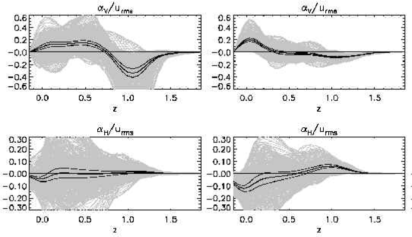
Figure 6.4: Vertical and horizontal components of the $\alpha$ effect. The gray lines represent different times, the thick line is the time average, and the surrounding thin curves indicate the error of the mean. The simulation is carried out on the southern hemisphere. The convection zone proper is in the range $0<z<1$, where $z$ denotes depth. The lower overshoot layer is in $z>1$ and the top overshoot layer is in $z<0$. In the upper parts of the convection zone ($0<z<0.6$) the vertical component of $\alpha_{\rm V}\equiv\alpha_{zz}$ is positive (upper panels) while the horizontal components, $\alpha_{\rm H}\equiv\alpha_{xx}=\alpha_{yy}$ are negative (lower panels). The left and right hand columns are for simulations with different angular velocity: slower on the left (the Taylor number is $2\times 10^{3}$) and faster on the right (the Taylor number is $10^{4}$). Courtesy M. Ossendrijver [308].

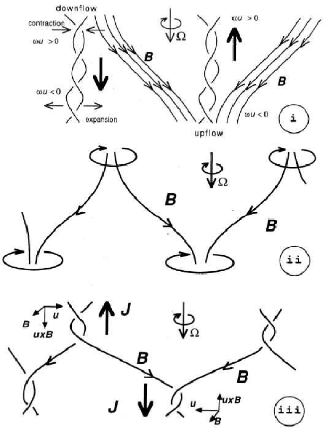
Figure 6.5: Sketch showing the twisting of vertical magnetic field lines by downdrafts. The resulting electromotive force, $\mbox{\boldmath${\cal E}$}{}=\bm{u}\times\bm{b}$, points in the direction of the mean field, giving a positive $\alpha_{\rm V}$ in the southern hemisphere and a negative $\alpha_{\rm V}$ in the northern hemisphere. Adapted from Ref. [307].

Two surprising results emerged from the simulations. In convection the $\alpha$ effect is extremely anisotropic with respect to the vertical direction such that the diagonal components of $\alpha_{ij}$ can even change sign. While the horizontal components, $\alpha_{xx}$ and $\alpha_{yy}$, show the expected sign and are roughly a negative multiple of the kinetic helicity, the vertical component, $\alpha_{zz}$, shows invariably the opposite sign [307, 308]; see Fig. 6.4. This peculiar result can be understood by noting that vertical field lines are wrapped around each other by individual downdrafts, which leads to field line loops oppositely oriented than if they were caused by an expanding updraft.

In Fig. 6.5 we show the field line topology relevant to the situation in the southern hemisphere. The degree of stratification is weak, so the downdrafts at the top look similar to the updrafts at the bottom (both are indicated by two swirling lines). (i) At the top and bottom boundaries the magnetic field is concentrated in the intergranular lanes which correspond to downdrafts at the top and updrafts at the bottom. (ii) This leads to a clockwise swirl both at the top and at the bottom (but counter-clockwise in the northern hemisphere); see the second panel. (iii) This in turn causes left-handed current helicity in the upper parts and right-handed current helicity in the lower parts, so one might expect that $\alpha$ is negative in the upper parts and positive in the lower parts. This is however not the case. Instead, what really matters is $\mbox{\boldmath${\cal E}$}{}=\bm{u}\times\bm{b}$, where $\bm{u}$ is dominated by converging motions (both at the top and the bottom). This, together with $\bm{b}$ winding in the counter-clockwise direction around the downdraft and in the clockwise direction in the updraft, causes $\bm{u}\times\bm{b}$ to point in the direction of $\overline{\bm{B}}$ at the top (so $\alpha_{zz}$ is positive) and in the opposite direction at the bottom (so $\alpha_{zz}$ is negative). Originally, this result was only obtained for weak stratification [307], but meanwhile it has also been confirmed for strong stratification [308]. We reiterate that a qualitatively similar result has also been obtained in analytic calculations of the $\alpha$ effect from supernova-driven expanding shells in the stratified galactic disc [309] and in FOSA calculations of stratified turbulence [310].

Figure 6.6: The latitudinal dependence of the three components of the pumping velocity ($\theta=0$ corresponds to the south pole and $\theta=90$ to the equator). The vertical pumping velocity ($\gamma_{z}$, right-most panel) is positive, corresponding to downward pumping, and almost independent of latitude. The two horizontal components of $\bm{\gamma}$ vanish at the poles. The longitudinal pumping velocity ($\gamma_{y}$, middle panel) is negative, corresponding to retrograde pumping, and the latitudinal pumping velocity ($\gamma_{x}$, left panel) is positive, corresponding to equatorward pumping. Adapted from Ref. [334].

The other surprising result is that the turbulent pumping is not necessarily restricted to the vertical direction, but it can occur in the other two directions as well. In general one can split the $\alpha_{ij}$ tensor into symmetric and antisymmetric components, i.e. $\alpha_{ij}=\alpha_{ij}^{\rm(S)}+\alpha_{ij}^{\rm(A)}$, where the antisymmetric components can be expressed in the form

$$\alpha_{ij}^{\rm(A)}=-\epsilon_{ijk}\gamma_{k},$$ (6.25)

where $\bm{\gamma}$ is the pumping velocity. We recall that $\alpha_{ij}^{\rm(A)}\overline{B}_{j}=(\bm{\gamma}\times\overline{\bm{B}})_{i}$, which looks like the induction term $\overline{\mbox{\boldmath$U$}}\times\overline{\bm{B}}$, so $\bm{\gamma}$ acts like an advection velocity. Simulations show that $\bm{\gamma}$ has a component pointing in the retrograde direction; see Fig. 6.6 and Ref. [334]. We shall return to the theory of this term in Section 10.3; see Eq. (10.64).

The latitudinal component of the pumping velocity points toward the equator and has been invoked to explain the equatorward migration seen in the butterfly diagram [335]. The equatorward pumping was found to act mostly on the toroidal component of the mean field while the poloidal field was found to experience a predominantly poleward pumping velocity. This result has also been confirmed using simulations of turbulent convection [334].

A general problem with all these calculations is that, as the Reynolds number is increased, the fluctuations in $\overline{\mbox{\boldmath${\mathcal{E}}$}}{}$ become large and long integration times are necessary [311]. This is related to the problem that for large values of $R_{\rm m}$, small scale dynamo action becomes possible and, unless the imposed field is strong enough, the resulting values of $\overline{\mbox{\boldmath${\mathcal{E}}$}}{}$ are only weakly linked to $\bm{B}_{0}$. Indeed, $\overline{\mbox{\boldmath${\mathcal{E}}$}}{}$ will be dominated by a rather strong noise component, making it necessary to calculate long time averages to extract a small average from the strongly fluctuating component.

6.4.2 Test field procedure with finite gradients

A general procedure for determining the full $\alpha_{ij}$ and $\eta_{ijk}$ tensors from a simulation is to calculate the electromotive force after applying test fields of different directions and with different gradients [336]. There are altogether $9+27$ unknowns, if the mean field can vary in all three directions, or $9+18$ unknowns, if it can vary only in 2 directions (as is the case for toroidal or $y$ averages, for example). The idea is to calculate the emf,

$$\overline{\mbox{\boldmath${\mathcal{E}}$}}{}^{(q)}=\overline{\bm{u}\times\bm{b}^{(q)}},$$ (6.26)

for the excess magnetic fluctuations, $\bm{b}^{(q)}$, that are due to a given test field $\overline{\bm{B}}^{(q)}$. This requires solving simultaneously a set of equations of the form

$${\partial\bm{b}^{(q)}\over\partial t}=\bm{\nabla}\times\left[\left(\overline{\mbox{\boldmath$U$}}+\bm{u}\right)\times\overline{\bm{B}}^{(q)}\right]+\eta\nabla^{2}\bm{b}^{(q)}+\bm{G}$$ (6.27)

for each test field $\overline{\bm{B}}^{(q)}$. Here, the mean flow $\overline{\mbox{\boldmath$U$}}$ has been retained and $\bm{G}=\bm{\nabla}\times[\bm{u}\times\bm{b}^{(q)}-\overline{\bm{u}\times\bm{b}^{(q)}}]$ is a term nonlinear in the fluctuation. This term would be ignored in the first order smoothing approximation, but it can be kept in a simulation if desired. For two-dimensional averages, for example, one has $9+18=27$ unknowns, so one needs 9 test fields $\overline{\bm{B}}^{(q)}$ to calculate 9 vectors $\overline{\mbox{\boldmath${\mathcal{E}}$}}{}^{(q)}$. Expressing ${\cal E}_{i}^{(q)}$ in the form

$$\overline{\mbox{\boldmath${\mathcal{E}}$}}{}^{(q)}=\alpha_{ij}\overline{B}^{(q)}_{j}+\eta_{ijk}\overline{B}_{j,k}^{(q)},$$ (6.28)

one arrives at a system of 27 equations for the 27 unknowns.

By choosing 3 of the test fields to be constants, one can first solve for the 9 unknowns $\alpha_{ij}$. The remaining coefficients in $\eta_{ijk}$ can then be obtained by choosing test fields that vary linearly as a function of space. This type of analysis has been applied successfully to laminar stationary convection in a sphere exhibiting a dynamo effect [336]. In this special case no matrix inversion is necessary. However, in addition to problems with boundary conditions, there is the difficulty that $\alpha_{ij}$ and $\eta_{ijk}$ may be wavenumber dependent, so it may be better to choose only test fields with similar spatial variation (or wavenumber). In that case one needs to invert simple $2\times 2$ matrices with coefficients that depend on the test fields and their gradients.

Another remotely related method is to use a time-dependent magnetic field in a successful turbulent (nonstationary) dynamo simulation. The hope is here that the resulting mean magnetic field covers a substantial fraction of the parameter space allowing one to calculate meaningful moments of the form $\langle\overline{\cal E}_{i}\overline{B}_{j}\rangle$ and $\langle\overline{\cal E}_{i}\overline{B}_{j,k}\rangle$. Using a general representation of $\overline{\mbox{\boldmath${\mathcal{E}}$}}{}$ of the form Eq. (6.9) allows one to calculate the transport coefficients $\alpha_{ij}$ and $\eta_{ijk}$ by inverting suitable correlation matrices. This method has been applied with modest success to the problem of large scale field generation in a local model of accretion disc turbulence [337, 338].

6.4.3 Comparison of simulations with theory

Whenever a meaningful comparison between simulations and theory (FOSA) is possible, the agreement can be quite remarkable. An example where this is the case is laminar convection in a rotating spherical shell, where the velocity field from the simulation has been inserted into the corresponding mean-field expressions [336].

In the case of turbulent convection, where only the turbulent rms velocity is used to scale theory to simulations, the agreement is merely on a qualitative level. One obvious property of simulated values of $\alpha$ is the high degree of fluctuations [311]. This is because here mean fields are defined as spatial averages. Fluctuations of the turbulent transport coefficients are normally ignored when ensemble averages are used [339]. As a general trend one can note that theory tends to overestimate the magnitudes of $\alpha$, $\gamma$, and $\eta_{\rm t}$. This can partly be explained as a consequence of catastrophic (i.e. magnetic Reynolds number dependent) quenching [308]. This will be discussed in detail later in this review; see Section 9.3. For now, let us note that the catastrophic quenching became particularly obvious in simulations of isotropic homogeneous turbulence in a fully periodic box [340]. Agreement between theory and simulations was only achieved when the dynamical quenching formalism was used [6]. Historically, of course, neither the dynamical quenching nor the corresponding helicity fluxes were known. Therefore, any agreement between simulations and theory was only a consequence of having adopted sufficiently small a magnetic Reynolds number or, possibly, of magnetic or current helicity fluxes having been quite efficient, so that the effect of dynamical quenching became less restrictive.

An outstanding question where much more work needs to be done is indeed the issue of current helicity fluxes. They will be discussed in more detail below (Sections 8.11, 9.6, 9.7, 10.4). Their calculation is just as important as that of the other transport coefficients, because these fluxes help alleviating the otherwise catastrophic quenching.

6.5 $\alpha^{2}$ and $\alpha\Omega$ dynamos: simple solutions

For astrophysical purposes one is usually interested in solutions in spherical or oblate (disc-like) geometries. However, in order to make contact with turbulence simulations in a periodic box, solutions in simpler cartesian geometry can be useful. Cartesian geometry is also useful for illustrative purposes. In this subsection we review some simple cases.

Mean field dynamos are traditionally divided into two groups; $\alpha\Omega$ and $\alpha^{2}$ dynamos. The $\Omega$ effect refers to the amplification of the toroidal field by shear (i.e. differential rotation) and its importance for the sun was recognized very early on. Such shear also naturally occurs in disk galaxies, since they are differentially rotating systems [210]. However, it is still necessary to regenerate the poloidal field. In both stars and galaxies the $\alpha$ effect is the prime candidate. This explains the name $\alpha\Omega$ dynamo; see the left hand panel of Fig. 6.7. However, large scale magnetic fields can also be generated by the $\alpha$ effect alone, so now also the toroidal field has to be generated by the $\alpha$ effect, in which case one talks about an $\alpha^{2}$ dynamo; see the right hand panel of Fig. 6.7. (The term $\alpha^{2}\Omega$ model is discussed at the end of Section 6.5.2.)

Figure 6.7: Mutual regeneration of poloidal and toroidal fields in the case of the $\alpha\Omega$ dynamo (left) and the $\alpha^{2}$ dynamo (right).

6.5.1 $\alpha^{2}$ dynamo in a periodic box

We assume that there is no mean flow, i.e. $\overline{\mbox{\boldmath$U$}}=0$, and that the turbulence is homogeneous, so that $\alpha$ and $\eta_{\rm t}$ are constant. The mean field induction equation then reads

$${\partial\overline{\bm{B}}\over\partial t}=\alpha\bm{\nabla}\times\overline{\bm{B}}+\eta_{\rm T}\nabla^{2}\overline{\bm{B}},\quad\bm{\nabla}\cdot\overline{\bm{B}}=0,$$ (6.29)

where $\eta_{\rm T}=\eta+\eta_{\rm t}$ is the sum of microscopic and turbulent magnetic diffusivity. We can seek solutions of the form

$$\overline{\bm{B}}(\bm{x})=\mbox{Re}\left[\hat{\bm{B}}(\bm{k})\,\exp(\mathrm{i}\bm{k}\cdot\bm{x}+\lambda t)\right].$$ (6.30)

This leads to the eigenvalue problem $\lambda\hat{\bm{B}}=\alpha\mathrm{i}\bm{k}\times\hat{\bm{B}}-\eta_{\rm T}k^{2}\hat{\bm{B}}$, which can be written in matrix form as

$$\lambda\hat{\bm{B}}=\pmatrix{-\eta_{\rm T}k^{2}&-\mathrm{i}\alpha k_{z}&\mathrm{i}\alpha k_{y}\cr\mathrm{i}\alpha k_{z}&-\eta_{\rm T}k^{2}&-\mathrm{i}\alpha k_{x}\cr-\mathrm{i}\alpha k_{y}&\mathrm{i}\alpha k_{x}&-\eta_{\rm T}k^{2}}\hat{\bm{B}}.$$ (6.31)

This leads to the dispersion relation, $\lambda=\lambda(\bm{k})$, given by

$$(\lambda+\eta_{\rm T}k^{2})\left[(\lambda+\eta_{\rm T}k^{2})^{2}-\alpha^{2}k^{2}\right]=0,$$ (6.32)

with the three solutions

$$\lambda_{0}=-\eta_{\rm T}k^{2},\quad\lambda_{\pm}=-\eta_{\rm T}k^{2}\pm|\alpha k|.$$ (6.33)

The eigenfunction corresponding to the eigenvalue $\lambda_{0}=-\eta_{\rm T}k^{2}$ is proportional to $\bm{k}$, but this solution is incompatible with solenoidality and has to be dropped. The two remaining branches are shown in Fig. 6.8.

Figure 6.8: Dispersion relation for $\alpha^{2}$ dynamo, where $k_{\rm crit}=\alpha/\eta_{\rm T}$.

Unstable solutions ($\lambda>0$) are possible for $0<\alpha k<\eta_{\rm T}k^{2}$. For $\alpha>0$ this corresponds to the range

$$0<k<\alpha/\eta_{\rm T}\equiv k_{\rm crit}.$$ (6.34)

For $\alpha<0$, unstable solutions are obtained for $k_{\rm crit}<k<0$. The maximum growth rate is at

$$k_{\max}={\textstyle{1\over 2}}k_{\rm crit}=\alpha/(2\eta_{\rm T})\quad\quad\mbox{(maximum growth rate)}.$$ (6.35)

Such solutions are of some interest, because they have been seen as an additional hump in the magnetic energy spectra from fully three-dimensional turbulence simulations (Sections 8.4 and 8.6).

Linear theory is only applicable as long as the magnetic field is weak, but qualitatively one may expect that in the nonlinear regime $\alpha$ becomes reduced (quenched), so $k_{\rm crit}$ decreases and only larger scale magnetic fields can be maintained. This is indeed seen in numerical simulations [4]; see also Section 8.

6.5.2 $\alpha\Omega$ dynamo in a periodic box

Next we consider the case with linear shear, and assume $\overline{\mbox{\boldmath$U$}}=(0,Sx,0)$, where $S=\mbox{const}$. This model can be applied as a local model to both accretion discs ($x$ is radius, $y$ is longitude, and $z$ is the height above the midplane) and to stars ($x$ is latitude, $y$ is longitude, and $z$ is radius). For keplerian discs, the shear is $S=-{3\over 2}\Omega$, while for the sun (taking here only radial differential rotation into account) $S=r\partial\Omega/\partial r\approx+0.1\Omega_{\odot}$ near the equator.

For simplicity we consider axisymmetric solutions, i.e. $k_{y}=0$. The eigenvalue problem takes then the form

$$\lambda\hat{\bm{B}}=\pmatrix{-\eta_{\rm T}k^{2}&-\mathrm{i}\alpha k_{z}&0\cr\mathrm{i}\alpha k_{z}+S&-\eta_{\rm T}k^{2}&-\mathrm{i}\alpha k_{x}\cr 0&\mathrm{i}\alpha k_{x}&-\eta_{\rm T}k^{2}}\hat{\bm{B}},$$ (6.36)

where $\eta_{\rm T}=\eta+\eta_{\rm t}$ and $\bm{k}^{2}=k_{x}^{2}+k_{z}^{2}$. The dispersion relation is now

$$(\lambda+\eta_{\rm T}k^{2})\left[(\lambda+\eta_{\rm T}k^{2})^{2}+\mathrm{i}\alpha Sk_{z}-\alpha^{2}k^{2}\right]=0,$$ (6.37)

with the solutions

$$\lambda_{\pm}=-\eta_{\rm T}k^{2}\pm(\alpha^{2}k^{2}-\mathrm{i}\alpha Sk_{z})^{1/2}.$$ (6.38)

Again, the eigenfunction corresponding to the eigenvalue $\lambda_{0}=-\eta_{\rm T}k^{2}$ is not compatible with solenoidality and has to be dropped. The two remaining branches are shown in Fig. 6.9, together with the approximate solutions (valid for $\alpha k_{z}/S\ll 1$)

$$\mbox{Re}\lambda_{\pm}\approx-\eta_{\rm T}k^{2}\pm|{\textstyle{1\over 2}}\alpha Sk_{z}|^{1/2},$$ (6.39)

$$\mbox{Im}\lambda_{\pm}\equiv-\omega_{\rm cyc}\approx\pm|{\textstyle{1\over 2}}\alpha Sk_{z}|^{1/2},$$ (6.40)

where we have made use of the fact that $\mathrm{i}^{1/2}=(1+\mathrm{i})/\sqrt{2}$.

Figure 6.9: Dispersion relation for $\alpha^{2}\Omega$ dynamo with $\alpha k_{\rm crit}/S=0.35$. The dotted line gives the result for the $\alpha\Omega$ approximation Eqs. (6.39) and (6.40). The axes are normalized using $k_{\rm crit}$ for the full $\alpha^{2}\Omega$ dynamo equations.

Sometimes the term $\alpha^{2}\Omega$ dynamo is used to emphasize that the $\alpha$ effect is not neglected in the generation of the toroidal field. This approximation, which is sometimes also referred to as the $\alpha\Omega$ approximation, is generally quite good provided $\alpha k_{z}/S\ll 1$. However, it is important to realize that this approximation can only be applied to axisymmetric solutions [341].

6.5.3 Eigenfunctions, wave speed, and phase relations

We now make the $\alpha\Omega$ approximation and consider the marginally excited solution ($\mbox{Re}\lambda=0$), which can be written as

$$\overline{B}_{x}=B_{0}\sin k_{z}(z-ct),\quad\overline{B}_{y}=\sqrt{2}\,B_{0}\left|{c\over\alpha}\right|\sin[k_{z}(z-ct)+\varphi],$$ (6.41)

where $B_{0}$ is the amplitude (undetermined in linear theory), and $c=\omega_{\rm cyc}/k_{z}$ is the phase speed of the dynamo wave, which is given by

$$c={\alpha S\over|2\alpha Sk_{z}|^{1/2}}=\pm\eta_{\rm T}k_{z},$$ (6.42)

where the upper (lower) sign applies when $\alpha S$ is positive (negative). The sign of $c$ gives the direction of propagation of the dynamo wave; see Table LABEL:Tpropagation for a summary of the propagation directions in different settings.

Table 6.2: Summary of propagation directions and phase relation for $\alpha\Omega$ dynamos.

object $\alpha$ $S$ $\varphi$ $c$ wave propagation $|\omega_{\rm cyc}|\,\Delta t$ disc $-$ $-$ $-3\pi/4$ $+$ away from midplane $-3\pi/4$ disc/star? $+$ $-$ $+3\pi/4$ $-$ equatorward $-3\pi/4$ star? $-$ $+$ $-\pi/4$ $-$ equatorward $+\pi/4$ star $+$ $+$ $+\pi/4$ $+$ poleward $+\pi/4$

An important property of the $\alpha\Omega$ dynamo solutions that can be read off from the plane wave solutions is the phase shift of $\pm{3\over 4}\pi$ (for $S<0$) and $\pm\pi/4$ (for $S>0$) between the poloidal and toroidal fields. It is customary [342, 343] to quote instead the normalized time delay $|\omega_{\rm cyc}|\,\Delta t=\varphi\,{\rm sgn}{}(c)$, by which the toroidal field lags behind the radial field. These values are given in the last column of Table LABEL:Tpropagation. Note that the temporal phase shift only depends on the sign of the shear $S$ and not on $\alpha$.

6.5.4 Excitation conditions in a sphere

For applications to stars it is essential to employ spherical geometry. Over the past three decades, a number of two-dimensional and three-dimensional models have been presented [298, 344, 345, 346]. The dynamo is generally characterized by two dynamo numbers,

$$C_{\alpha}=\alpha_{0}R/\eta_{\rm T},\quad C_{\Omega}=\Delta\Omega R^{2}/\eta_{\rm T},$$ (6.43)

where $\alpha_{0}$ and $\Delta\Omega$ are typical values of $\alpha$ and angular velocity difference across the sphere, and $R$ is the outer radius of the sphere. In Fig. 6.10 we show the critical values of $C_{\alpha}$ (above which dynamo action is possible) for different values of $C_{\Omega}$ using error function profiles,

$$f_{\pm}(r;r_{0},d)={\textstyle{1\over 2}}\left\{1\pm{\rm erf}\left[(r-r_{0})/d\right]\right\},$$ (6.44)

for $\alpha(r,\theta)=\alpha_{0}f_{+}(r;r_{\alpha},d_{\alpha})\cos\theta$ and $\Omega(r)=\Delta\Omega f_{-}(r;r_{\Omega},d_{\Omega})$, just as in the early work of Steenbeck and Krause [298], who used $r_{\alpha}=0.9$, $r_{\Omega}=0.7$, and $d_{\alpha}=d_{\Omega}=0.075$. On $r=R$ the field is matched to a potential field. A detailed presentation of the induction equation in spherical harmonics with differential rotation, meridional circulation, anisotropic $\alpha$ effect and a number of other effects is given by Rädler [347].

The solutions are classified by the symmetry properties about the equator (S and A for symmetric and antisymmetric fields, respectively), supplemented by the spherical harmonic degree $m$ characterizing the number of nodes in the azimuthal direction. Note that for axisymmetric modes (S0 and A0) the critical value of $C_{\alpha}$ decreases if $C_{\Omega}$ increases, while for the nonaxisymmetric modes (e.g. S1 and A1) $C_{\alpha}$ is asymptotically independent of $C_{\Omega}$. This behavior for S0 and A0 is understandable because for axisymmetric modes the excitation condition only depends on the product of $\alpha$ effect and shear; see Eq. (6.39). For S1 and A1, on the other hand, differential rotation either makes the dynamo harder to excite (if $C_{\Omega}$ is small) or it does not affect the dynamo at all (larger $C_{\Omega}$). This is because when differential rotation winds up a nonaxisymmetric field, anti-aligned field lines are brought close together [341]. For sufficiently large values of $C_{\Omega}$ the field is expelled into regions with no differential rotation ($\alpha^{2}$ dynamo) where the dynamo is essentially independent of $C_{\Omega}$.

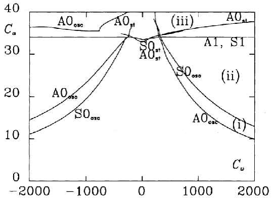
Figure 6.10: Critical values of $C_{\alpha}$ versus $C_{\omega}$ for a dynamo in a spherical shell. Note that near $C_{\omega}=200$ the nonaxisymmetric modes S1 and A1 are more easily excited than the axisymmetric modes S0 and A0. Here, $C_{\omega}$ (called $C_{\Omega}$ in the rest of this review) is defined such that it is positive when $\partial\Omega/\partial r$ is negative, and vice versa. Adapted from [346].

Generally, axisymmetric modes are easier to excite than nonaxisymmetric modes. There can be exceptions to this just at the junction between $\alpha^{2}$ and $\alpha\Omega$ dynamo behavior. This is seen near $C_{\omega}=300$; see Fig. 6.10. Such behavior was first reported by Robert and Stix [344], and may be important for understanding the occurrence of nonaxisymmetric fields in active stars; see Section 11.3. Other potential agents facilitating nonaxisymmetric fields include anisotropic [348, 349] and nonaxisymmetric [350, 351] forms of $\alpha$ effect and turbulent diffusivity.

Finally we note that for strong shear (large values of $|C_{\Omega}|$), and $\alpha>0$ in the northern hemisphere, the most easily excited modes are A0 (when $\partial\Omega/\partial r$ is negative, i.e. $C_{\omega}>0$ in Fig. 6.10), and S0 (when $\partial\Omega/\partial r$ is positive). This behavior changes the other way around, however, when the dynamo operates in a shell whose ratio of inner to outer shell radius exceeds a value of about 0.7 [352, 353]. This is approximately the appropriate value for the sun, and it has indeed long been recognized that the negative parity of the solar dynamo is not always obtained from model calculations [354, 355, 356].

6.5.5 Excitation conditions in disc-like geometries

Another important class of astrophysical bodies are galactic discs as well as discs around young stars, compact objects, or supermassive black holes in the nuclei of active galaxies; see Section 2.3. We consider the simplest form of the axisymmetric mean field dynamo equations appropriate for a thin disc [77],

$$\dot{\overline{B}}_{R}=-(\alpha\overline{B}_{\phi})^{\prime}+\eta_{\rm T}\overline{B}_{R}^{\prime\prime},\quad\dot{\overline{B}}_{\phi}=S\overline{B}_{R}+\eta_{\rm T}\overline{B}_{\phi}^{\prime\prime}.$$ (6.45)

Here, radial derivatives have been neglected, so the problem has become one-dimensional and can be solved separately at each radius. Primes and dots denote $z$ and $t$ derivatives, respectively, $\alpha=\alpha_{0}f_{\alpha}(z)$ is a profile for $\alpha$ (asymmetric with respect to $z=0$) with typical value $\alpha_{0}$, $S=R\mathrm{d}\Omega/\mathrm{d}R$ is the radial shear in the disc, and $(\overline{B}_{R},\overline{B}_{\phi},\overline{B}_{z})$ are the components of the mean field $\overline{\bm{B}}$ in cylindrical coordinates. On $z=\pm H$ one assumes vacuum boundary conditions which, in this one-dimensional problem, reduce to $\overline{B}_{R}=\overline{B}_{\phi}=0$. One can also impose boundary conditions on the mid-plane, $z=0$, by selecting either symmetric (quadrupolar) fields, $B_{R}=\overline{B}_{\phi}^{\prime}=0$, or antisymmetric (dipolar) fields, $B_{R}^{\prime}=\overline{B}_{\phi}=0$. One can again define two dimensionless control parameters,

$$C_{\Omega}=Sh^{2}/\eta_{\rm T},\quad C_{\alpha}=\alpha_{0}h/\eta_{\rm T},$$ (6.46)

which measure the strengths of shear and $\alpha$ effects, respectively, where $h$ is a measure of the disc scale height. (Note that $C_{\Omega}$ and $C_{\alpha}$ used here are akin to those defined in Section 6.5.4 and are identical to the symbols $R_{\Omega}$ and $R_{\alpha}$ commonly used in galactic dynamo literature.) In spiral galaxies, the typical values are $C_{\Omega}\approx-10$ and $C_{\alpha}\approx 1$, and so $|C_{\Omega}|\gg C_{\alpha}$.

Since $|C_{\Omega}|\gg C_{\alpha}$, dynamo generation of axisymmetric solutions is controlled by the dynamo number $D=C_{\Omega}C_{\alpha}$. Exponential growth of the fields is possible in the kinematic stage provided $|D|>D_{\rm crit}$. Here the critical dynamo number $D_{\rm crit}\sim 6$–$10$, depending on the exact profile adopted for the $\alpha(z)$. Here we assume $f_{\alpha}(z)=z/H$, where $H$ is the disc scale height. For negative $\partial\Omega/\partial R$ and positive values of $\alpha$ in the upper disc plane (northern ‘hemisphere’), the most easily excited modes are no longer A0, but S0 [222]. This case is believed to be relevant to galaxies and one expects that the most easily excited solutions for galaxies, are modes with steady quadrupole (S0 st) symmetry in the meridional ($Rz$) plane [77]. For these modes, the growth rate in the kinematic regime can be approximated by,

$$\gamma\approx{\eta_{\rm T}\over h^{2}}\left(\sqrt{|D|}-\sqrt{D_{\rm crit}}\right).$$ (6.47)

In most spiral galaxies the dynamo is supercritical for a large range of radii, and so galactic fields can indeed grow exponentially from small seed values. A detailed discussion of the properties of solutions in the galactic context is given in Ref. [77].

Further, as discussed in Section 6.5.4, axisymmetric modes are easier to excite than nonaxisymmetric ones. Although, the observed nonaxisymmetric large scale mean field structures in some galaxies, can also be explained by invoking nonaxisymmetric forms of $\alpha$ effect [350], turbulent diffusivity, or streaming motions [357, 358, 359].

For accretion discs, $\alpha$ might be negative in the northern hemisphere [201] and one therefore expects oscillatory quadrupoles (S0 osc) [360]. In Fig. 6.11 we show the growth rate of different modes, obtained by solving Eq. (6.45) for both signs of the dynamo number [360]. In order to find all the modes, even the unstable ones, one can easily solve Eq. (6.45) numerically as an eigenvalue problem, $\lambda\bm{q}=\mbox{\boldmath${\sf M}$}{}\bm{q}$, where the complex growth rate $\lambda$ is the eigenvalue with the largest real part.

For illustrative purposes, we discuss the numerical technique in detail. We introduce mesh points, $z_{i}=i\,\delta z$ (excluding the boundaries at $z=0$ and $z=H$), where $\delta z=H/(N+1)$ is the mesh spacing, and $i=1,2,...,N$ denotes the position on the mesh. The discretized eigenvector is

$$\bm{q}=(\overline{B}_{R1},\overline{B}_{\phi 1},\overline{B}_{R2},\overline{B}_{\phi 2},...,\overline{B}_{RN},\overline{B}_{\phi N})^{T}.$$ (6.48)

It is convenient to introduce the abbreviations $a_{i}=-\alpha_{i}/(2\delta z)$ and $b=\eta_{\rm T}/(\delta z)^{2}$, so then the second-order accurate discretized form of Eq. (6.45) reads

$$\dot{\overline{B}}_{R\,i}=a_{i+1}\overline{B}_{\phi\,i+1}-a_{i-1}\overline{B}_{\phi\,i-1}+b(\overline{B}_{R\,i+1}-2\overline{B}_{R\,i}+\overline{B}_{R\,i-1}),\quad$$ (6.49)

$$\dot{\overline{B}}_{\phi\,i}=S\overline{B}_{R\,i}+b(\overline{B}_{\phi\,i+1}-2\overline{B}_{\phi\,i}+\overline{B}_{\phi\,i-1}),$$ (6.50)

where $\alpha_{1}$, $\alpha_{2}$, …, are the values of $\alpha$ at the different mesh points. Using symmetric boundary conditions on $z=0$, we have $B_{R\,0}=0$ and $B_{\phi\,0}^{\prime}=(-3B_{\phi\,0}+4B_{\phi 1}-B_{\phi 2})/(2\delta z)=0$, which is just the second order one-sided first derivative formula [272]. With this we can eliminate the boundary point $B_{\phi\,0}={\textstyle{1\over 3}}(4B_{\phi 1}-B_{\phi 2})$, and have, in matrix form,

$$\mbox{\boldmath${\sf M}$}{}=\pmatrix{-2b&-{\textstyle{4\over 3}}a_{0}&b&{\textstyle{1\over 3}}a_{0}+a_{2}&0&0&0&0&...\cr S&-{\textstyle{2\over 3}}b&0&{\textstyle{2\over 3}}b&0&0&0&0&...\cr b&a_{1}&-2b&0&b&a_{3}&0&0&...\cr 0&b&S&-2b&0&b&0&0&...\cr 0&0&b&a_{2}&-2b&0&b&a_{4}&...\cr 0&0&0&b&S&-2b&0&b&...\cr...&...&...&...&...&...&...&...&...}.$$ (6.51)

In the lower right corner, no modification has to be applied, which then corresponds to the vacuum boundary condition $\overline{B}_{R}=\overline{B}_{\phi}=0$ on $z=\pm H$. For the results shown in Fig. 6.11 we have simply assumed a linear profile, i.e. $\alpha=\alpha_{0}z/H$, and $\eta_{\rm T}$ and $S$ are constant. The eigenvalues of the matrix ${\sf M}$ can be found using standard library routines.

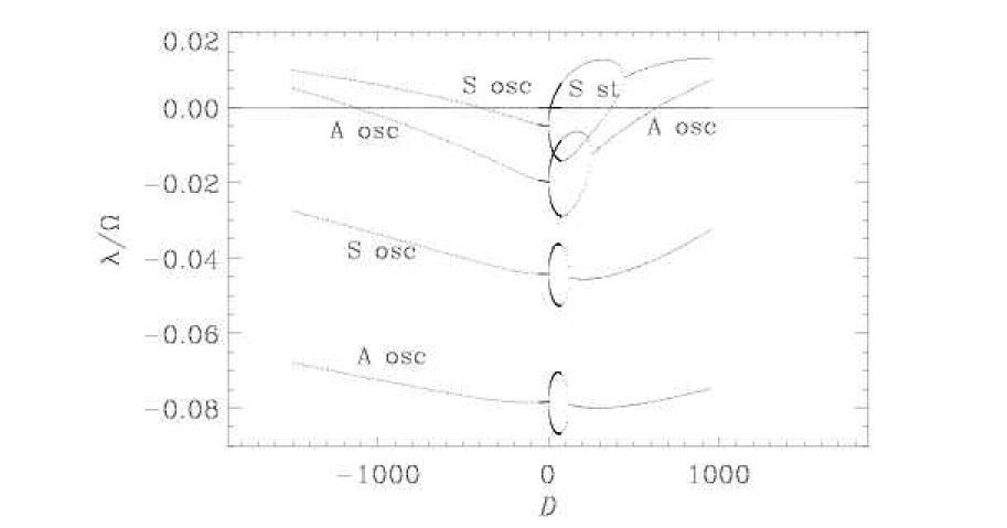
Figure 6.11: Eigenvalues of the dynamo equations with shear in slab geometry with radial shear. The dynamo number, in this figure, is defined positive when the shear in negative and $\alpha$ positive (opposite in sign to that in the text). Note that for $\alpha>0$ the solution that is most easily excited is nonoscillatory (‘steady’) and has even parity (referred to as S st) whilst for $\alpha<0$ it is oscillatory (S osc). Adapted from [360].

6.6 Rädler effect and shear–current effect

An important additional contribution to the EMF is a term of the form $\overline{\mbox{\boldmath${\mathcal{E}}$}}{}=...+\bm{\delta}\times\overline{\mbox{\boldmath$J$}}$. This term was first derived and identified as a possible dynamo generating term by Rädler [328], who found that in a rotating system with non-helical turbulence $\bm{\delta}$ is proportional to $\bm{\Omega}$. Even in a non-rotating system with linear shear alone, large scale dynamo action is possible due to the so-called shear–current effect [322, 323, 324], where $\bm{\delta}$ is proportional to the vorticity $\overline{\mbox{\boldmath$W$}}$ of the mean flow.

Figure 6.12: Dispersion relation for the $\delta^{2}S$ dynamo with $\delta k_{\rm crit}^{2}/S=0.2$. The dotted line gives the result for the “$\delta S$” approximation Eq. (6.54). The axes are normalized using $k_{\rm crit}$ as given by Eq. (6.53). Note the similarity to the dispersion relation for the $\alpha^{2}$ dynamo; cf. Fig. 6.8.

Numerous models with this effect have been considered in the early 1970ies [344, 348, 352]. Since this term does not give a contribution to $\overline{\mbox{\boldmath$J$}}\cdot\overline{\mbox{\boldmath${\mathcal{E}}$}}{}$, it cannot provide energy to the system. However, the presence of shear suffices to allow injection of energy into the system to offset resistive losses and hence to produce sustained large scale dynamo action. The dispersion relation for such an axisymmetric “$\delta S$” dynamo can easily be obtained from Eqs. (6.36) and (6.37) by replacing $\mathrm{i}\alpha\to\bm{k}\cdot\bm{\delta}$, and its solution is

$$\lambda_{\pm}=-\eta_{\rm T}k^{2}\pm[-(\bm{k}\cdot\bm{\delta})^{2}k^{2}-(\bm{k}\cdot\bm{\delta})Sk_{z}]^{1/2}.$$ (6.52)

Evidently, a necessary condition for growing solutions is that the term in square brackets is positive, and hence that $-Sk_{z}/(\bm{k}\cdot\bm{\delta})>k^{2}$. We refer to such solutions as “$\delta^{2}S$” dynamos, so as to emphasize that the $\bm{\delta}$ effect enters the regeneration of both poloidal and toroidal field. We use here the symbol $S$ instead of $\Omega$ to emphasize that angular velocity is unnecessary and that only shear is needed.

In the one-dimensional case with $\bm{k}=(0,0,k_{z})$ and $\bm{\delta}=(0,0,\delta)$, the necessary condition is $-\delta k_{z}^{2}/S>0$. Thus, for positive shear, growing solutions are only possible for negative values of $\delta$, and vice versa. The critical $k_{z}$ may then be obtained from Eq. (6.52) in the form

$$k_{\rm crit}=\left[-S\delta/(\delta^{2}+\eta_{\rm T}^{2})\right]^{1/2}.$$ (6.53)

The two solution branches are shown in Fig. 6.12, together with the solutions of the approximate dispersion relation, obtained by ignoring the $(\bm{k}\cdot\bm{\delta})^{2}k^{2}$ term inside the squared brackets of Eq. (6.52), i.e.

$$\lambda_{\pm}\approx-\eta_{\rm T}k^{2}\pm|-\delta Sk_{z}^{2}|^{1/2}\quad\mbox{(for $1\gg-\delta k_{z}^{2}/S>0$)}.$$ (6.54)

Note first of all that the approximate dispersion relation is fairly good even when $\delta k_{\rm crit}^{2}/S$ is not very small. Second, the approximation is formally equivalent to the dispersion relation for the $\alpha^{2}$ dynamo after replacing $|\alpha|\to|-\delta S|^{1/2}$.

7 Magnetic helicity conservation and inverse cascade

The mean field approach in terms of $\alpha$ effect and other turbulent transport coefficients has been quite popular in modeling the magnetic fields in various astrophysical bodies. Its main shortcoming is the rather simplistic treatment of turbulence. A very different approach has been pioneered by Frisch and coworkers [361] and explored quantitatively in terms of the Eddy Damped Quasi-Normal Markovian (EDQNM) closure approximation [304], which will be reviewed briefly below. In this approach, the main mechanism producing large scale fields is the inverse cascade of magnetic helicity toward larger scales. The $\alpha$ effect emerges in a self-consistent manner and, more importantly, the $\alpha$ effect is amended by a correction term proportional to the small scale current helicity which plays a crucial role in modern mean field theory (Section 9). We begin with an illustration of the inverse cascade mechanism using a simple 3-mode interaction model.

7.1 Inverse cascade in 3-mode interactions

The occurrence of an inverse cascade can be understood as the result of two waves (wavenumbers $\bm{p}$ and $\bm{q}$) interacting with each other to produce a wave of wavenumber $\bm{k}$. The following argument is due to Frisch et al. [361]. Assuming that during this process magnetic energy is conserved together with magnetic helicity, we have

$$M_{p}+M_{q}=M_{k},$$ (7.1)

$$|H_{p}|+|H_{q}|=|H_{k}|,$$ (7.2)

where we are assuming that only helicity of one sign is involved. Suppose the initial field is fully helical and has the same sign of magnetic helicity at all scales, we have

$$2M_{p}=p|H_{p}|\quad\mbox{and}\quad 2M_{q}=q|H_{q}|,$$ (7.3)

and so Eq. (7.1) yields

$$p|H_{p}|+q|H_{q}|=2M_{k}\geq k|H_{k}|,$$ (7.4)

where the last inequality is just the realizability condition (3.59) applied to the target wavenumber $\bm{k}$ after the interaction. Using Eq. (7.2) in Eq. (7.4) we have

$$p|H_{p}|+q|H_{q}|\geq k(|H_{p}|+|H_{q}|).$$ (7.5)

In other words, the target wavevector $\bm{k}$ after the interaction of wavenumbers $\bm{p}$ and $\bm{q}$ satisfies

$$k\leq{p|H_{p}|+q|H_{q}|\over|H_{p}|+|H_{q}|}.$$ (7.6)

The expression on the right hand side of Eq. (7.6) is a weighted mean of $p$ and $q$ and thus satisfies

$$\min(p,q)\leq{p|H_{p}|+q|H_{q}|\over|H_{p}|+|H_{q}|}\leq\max(p,q),$$ (7.7)

and therefore

$$k\leq\max(p,q).$$ (7.8)

In the special case where $p=q$, we have $k\leq p=q$, so the target wavenumber after interaction is always less or equal to the initial wavenumbers. In other words, wave interactions tend to transfer magnetic energy to smaller wavenumbers, i.e. to larger scale. This corresponds to an inverse cascade. The realizability condition, ${\textstyle{1\over 2}}k|H_{k}|\leq M_{k}$, was the most important ingredient in this argument. An important assumption that we made in the beginning was that the initial field be fully helical; see Ref. [159, 362] for the case of fractional helicity.

7.2 The EDQNM closure model

One of the earliest closure schemes applied to the MHD dynamo problem was the eddy-damped quasi-normal Markovian (EDQNM) approximation. This was worked out in detail by Pouquet, Frisch and Léorat (PFL) [304]. EDQNM has been used frequently when dealing with fluid turbulence and is described, for example, in Refs [325, 363]. We do not describe it in great detail. Instead, we outline just the basic philosophy, and the crucial insights gained from this closure. PFL assumed that the $\bm{b}$ and $\bm{u}$ fields were homogeneous, isotropic (but helical) random fields. This is similar to the unified treatment presented in Section 5.6. The large and small scale fields would again be distinguished by whether the wavenumber $k$ is smaller or greater than the wavenumber of the forcing. It was also assumed that the initial $\bm{b}$ field is statistically invariant under sign reversal ($\bm{b}\to-\bm{b}$); the MHD equations then preserve this property and the cross helicity $\langle\bm{u}\cdot\bm{b}\rangle$ is then always zero. Now suppose the MHD equations for the fluctuating fields are written symbolically as $\dot{u}=uu$, where $u$ stands for some component of $\bm{u}$ or $\bm{b}$ and $\langle u\rangle=0$. This notation is used only to illustrate the effects of the quadratic nonlinearity; the linear dissipative and forcing terms have been dropped since they do not pose any specific closure problem and can be re-introduced at the end. Then we obtain for the second and third moments, again in symbolic form,

$${d\langle uu\rangle\over dt}=\langle uuu\rangle,\quad{d\langle uuu\rangle\over dt}=\langle uuuu\rangle.$$ (7.9)

The quasi-normal approximation consists of replacing the fourth moment $\langle uuuu\rangle$ by its gaussian value, that is the sum of products of second order moments. It turns out that such an approximation leads to problems associated with unlimited growth of the third moment, and the violation of the positivity constraint for the energy spectra. This is cured by assuming that the neglected irreducible part of the fourth moment in (7.9) is in the form of a damping term, which is a suitable linear relaxation operator of the triple correlations (a procedure called eddy-damping). One also carries out ‘Markovianization’, by assuming that the third moment responds to the instantaneous product of the second moments. The resulting third moment is substituted back on the RHS of the equation for second moments in (7.9). This results in a closed equation for the equal-time second-order moments

$${d\langle uu\rangle\over dt}=\theta(t)\langle uu\rangle\langle uu\rangle,$$ (7.10)

where $\theta(t)$ essentially describes a relaxation time for a given triad of interacting modes. It is given by,

$$\theta(t)=\int_{0}^{t}\e^{-\int_{\tau}^{t}\mu(s)\,\mathrm{d}s}\,\mathrm{d}\tau.$$ (7.11)

Here $\mu(s)$ is the eddy damping operator and was written down in Ref. [304] using phenomenological considerations. It depends on the kinetic and magnetic spectrum and incorporates the damping effects on any mode due to nonlinear interactions, Alfven effect and microscopic diffusion. (In the stationary case, where $\mu=\mbox{constant}$, $\theta\to\mu^{-1}$.) The derived evolution equations for the energy and helicity spectra of the random velocity and magnetic fields, are shown to preserve the quadratic invariants of total energy and magnetic helicity, just as in full MHD. The complete spectral equations under the EDQNM approximation are give in Table I of Ref. [304], and will not be reproduced here (see also the Appendix in Ref. [364]).

However several crucial insights resulted from this work about how the Lorentz force affects the large scale dynamo. From the EDQNM evolution equations for the kinetic and magnetic spectra, PFL identified three important effects, all of which involve the coupling between widely separated scales. Suppose $M_{k}$ and $H_{k}$ are the magnetic energy and helicity spectra and $E_{k}$, $F_{k}$ the corresponding kinetic energy and helicity spectra. And suppose we are interested in the dynamics of the magnetic energy at wavenumber $k$ due to velocity and magnetic fields at much larger scales (wavenumbers $\leq a_{0}k$) and much smaller scales (wavenumber $\geq k/a_{0}$), where $a_{0}\ll 1$. Then, in concrete terms, PFL found that the nonlocal contributions to the evolution are

$$\dot{(M_{k})}_{\rm NLoc}=k\Gamma_{k}(E_{k}-M_{k})+\alpha^{R}k^{2}H_{k}-2\nu^{V}_{k}k^{2}M_{k}+\ldots,$$ (7.12)

$$\dot{(H_{k})}_{\rm NLoc}=(\Gamma_{k}/k)(F_{k}-k^{2}H_{k})+\alpha^{R}M_{k}-2\nu^{V}_{k}k^{2}H_{k}+\ldots,$$ (7.13)

$$\dot{(E_{k})}_{\rm NLoc}=-k\Gamma_{k}(E_{k}-M_{k})-2({\textstyle{2\over 5}}\nu^{V}_{k}+\nu^{M}_{k}+\nu^{R}_{k})k^{2}E_{k}+\ldots,$$ (7.14)

$$\dot{(F_{k})}_{\rm NLoc}=-k\Gamma_{k}(F_{k}-k^{2}H_{k})-2({\textstyle{2\over 5}}\nu^{V}_{k}+\nu^{M}_{k}+\nu^{R}_{k})k^{2}F_{k}+\ldots,$$ (7.15)

where

$$\Gamma_{k}={\textstyle{4\over 3}}k\int_{0}^{a_{0}k}\theta_{kkq}M_{q}\mathrm{d}q,$$ (7.16)

$$\alpha_{k}^{R}=-{\textstyle{4\over 3}}\int_{k/a_{0}}^{\infty}\theta_{kqq}\left[F_{k}-k^{2}H_{k}\right]\mathrm{d}q,\quad\nu^{V}_{k}={\textstyle{2\over 3}}\int_{k/a_{0}}^{\infty}\theta_{kqq}E_{q}\mathrm{d}q.$$ (7.17)

$$\nu^{M}_{k}={\textstyle{2\over 3}}\int_{k/a_{0}}^{\infty}\theta_{kqq}M_{q}\mathrm{d}q,\quad\nu^{R}_{k}={\textstyle{2\over 15}}\int_{k/a_{0}}^{\infty}\theta_{kqq}q{\partial\mu_{q}\over\partial q}(E_{q}-M_{q})\mathrm{d}q.$$ (7.18)

The first term on the RHS of (7.12), referred to by PFL as the Alfvén effect, leads to equipartition of the kinetic and magnetic energies, at any scale due to magnetic energy at larger scales. This happens on the Alfvén crossing time of the larger scale field. The second term, very important for what follows, shows that the growth of large scale magnetic energy is induced by the small scale ‘residual’ helicity, which is the difference between the kinetic helicity and a current helicity contribution, due to the small scale magnetic field. The part of $\alpha_{k}^{R}$ depending on the kinetic helicity corresponds closely to the usual $\alpha$ effect, once one realizes that $\theta$ is like a correlation time. Over and above this term PFL discovered for the first time the current helicity contribution, the $k^{2}H_{k}$ term in $\alpha_{k}^{R}$. The third term gives the turbulent diffusion of the large scale magnetic field. Surprisingly, this term does not get affected, to the leading order, by nonlinear effects of the Lorentz force (although the small scale magnetic field does affect the diffusion of the large scale velocity field). PFL also gave a heuristic derivation of the last two results, because of their potential importance. This derivation, has since been reproduced in various forms by several authors [222, 365, 366] and has also been extended to include higher order corrections [258]. We outline it in Appendix D and use it to discuss the nonlinear saturation of the large scale dynamo in Section 9.3.

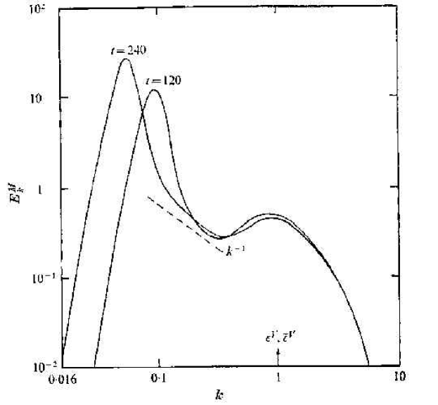
Figure 7.1: Inverse cascade in a numerical solution of the EDQNM equations showing the magnetic energy spectrum (here called $E_{k}^{\rm M}$) at two different times. Kinetic energy and helicity are injected at wavenumber $k=1$. Note the peak of magnetic energy propagating toward smaller values of $k$. Adapted from [304].

The EDQNM equations were numerically integrated by PFL to study the dynamo growth of magnetic energy. Most important in the present context is the case when both kinetic energy and helicity are continuously injected. In this case PFL found what they described as an inverse cascade of magnetic helicity, which led to the appearance of magnetic energy and helicity in ever increasing scales (limited only by the size of the system). Fig. 7.1 shows the resulting magnetic energy spectrum at two times. One can see the build up of large scale magnetic energy on scales much larger than the injection scale ($k=1$). PFL have also argued that this inverse cascade of magnetic energy resulted from a competition between the helicity (residual $\alpha$) and the Alfvén effect. We shall return to this question in subsequent sections. Numerical solutions to the EDQNM closure equations also reproduce small scale dynamo action in the absence of helicity [367]. However, the decisive terms describing small scale dynamo action do not seem to appear in the nonlocal interaction terms extracted in Eqs. (7.12)–(7.15).

8 Simulations of large scale dynamos

For astrophysical applications, the inverse cascade approach using the PFL model seemed too idealized compared to the $\alpha^{2}$ and $\alpha\Omega$ dynamo models that have been studied intensively in those years when the PFL model was proposed. Furthermore, there seems little scope for generalizing EDQNM to inhomogeneous systems with rotation. Nevertheless, the basic idea of an inverse cascade was well established and verified by several groups [4, 262, 368, 369, 370]. Only recently, however, there have been serious attempts to bridge the gap between the PFL approach and mean field models. In this section we review recent efforts [4] to study helically driven hydromagnetic turbulence and to compare with the associated $\alpha^{2}$ dynamo model that is applicable in the equivalent situation, i.e. also with fully periodic boundary conditions. After that, in Section 9, we consider in detail the implications of the conservation of magnetic helicity to mean field models.

8.1 The basic equations

In order to simulate the effect of cyclonic turbulence without actually including the physical effects that contribute to cyclonic turbulence one can substitute the buoyancy term by an explicit body force. The effects of stratification and rotation are therefore neglected.

A compressible isothermal gas with constant sound speed $c_{\rm s}$, constant dynamical viscosity $\mu$, and constant magnetic diffusivity $\eta$ is considered. To make sure the magnetic field stays solenoidal, i.e. $\bm{\nabla}\cdot\bm{B}=0$, $\bm{B}$ is expressed in terms of the magnetic vector potential $\bm{A}$, so the field is written as $\bm{B}=\bm{\nabla}\times\bm{A}$. The governing equations for density $\rho$, velocity $\bm{u}$, and magnetic vector potential $\bm{A}$, are given by

$${\mathrm{D}\ln\rho\over\mathrm{D}t}=-\bm{\nabla}\cdot\bm{u},$$ (8.1)

$${\mathrm{D}\bm{u}\over\mathrm{D}t}=-c_{\rm s}^{2}\bm{\nabla}\ln\rho+{\bm{J}\times\bm{B}\over\rho}+{\mu\over\rho}(\nabla^{2}\bm{u}+{\textstyle{1\over 3}}\bm{\nabla}\bm{\nabla}\cdot\bm{u})+\bm{f},$$ (8.2)

$${\partial\bm{A}\over\partial t}=\bm{u}\times\bm{B}+\eta\nabla^{2}\bm{A},$$ (8.3)

where ${\rm D}/{\rm D}t=\partial/\partial t+\bm{u}\cdot\bm{\nabla}$ is the advective derivative. The current density, $\bm{J}=\bm{\nabla}\times\bm{B}/\mu_{0}$, is obtained in the form $\mu_{0}\bm{J}=-\nabla^{2}\bm{A}+\bm{\nabla}\bm{\nabla}\cdot\bm{A}$. The gauge $\phi=-\eta\bm{\nabla}\cdot\bm{A}$ for the electrostatic potential is used, and $\eta=\mbox{constant}$ is assumed, so the magnetic diffusion term is just $\eta\nabla^{2}\bm{A}$. Details regarding the numerical solution of these equations are analogous to the nonhelical case and are discussed elsewhere [272]. Many of the simulations presented here have been done using the Pencil Code [271], mentioned already in Section 5.4.

For the following it is useful to recall that each vector field can be decomposed into a solenoidal and two vortical parts with positive and negative helicity, respectively. These are also referred to as Chandrasekhar-Kendall functions (cf. Section 3.7). It is often useful to decompose the magnetic field into positively and negatively helical parts. Here, we use eigenfunctions with positive eigenvalues (i.e. with positive helicity) as forcing function $\bm{f}$ of the flow. We restrict ourselves to functions selected from a finite band of wavenumbers around the wavenumber $k_{\rm f}$, but direction and amplitude are chosen randomly at each timestep. Further details can be found in Ref. [4]. Similar work was first carried out by Meneguzzi et al. [262], but at the time one was barely able to run even until saturation. Since the nineties, a lot of work has been done on turbulent dynamos with ABC flow-type forcing [226, 227, 229, 370]. In none of these investigations, however, the saturation behavior has been studied and so the issue of resistively slow magnetic helicity evolution past initial saturation remained unnoticed. It is exactly this aspect that has now become so crucial in understanding the saturation behavior of nonlinear dynamos. We begin by discussing first the linear (kinematic) evolution of the magnetic field.

8.2 Linear behavior

Dynamo action occurs once the magnetic Reynolds number exceeds a certain critical value, $R_{\rm crit}$. For helical flows, $R_{\rm crit}$ is between 1 and 2. Note that the values given in Table 1 of Ref. [4] need to be divided by $2\pi$ in order to conform with the definition of the magnetic Reynolds number, $R_{\rm m}=u_{\rm rms}/(\eta k_{\rm f})$, used throughout most of this review. In the supercritical case, $R_{\rm m}>R_{\rm crit}$, the field grows exponentially with the growth rate $\lambda$, which is proportional to the inverse turnover time, $u_{\rm rms}k_{\rm f}$. The resistively limited saturation behavior that will be discussed below in full detail has no obvious correspondence in the kinematic stage when the field is too weak to affect the motions by the Lorentz force [223]. Nevertheless, there is actually a subtle effect on the shape of the magnetic energy spectrum as $R_{\rm m}$ increases: the magnetic energy spectrum has two bumps, each being governed by opposite magnetic helicity. We will explain this in more detail below, where we also show the evolution of the two bumps (Fig. 8.2). For now we just note that, while in the weakly supercritical case the two bumps can be far apart from each other. However, as $R_{\rm m}$ is increased the two bumps in the spectra move closer together while maintaining a similar height, decreasing thus the net magnetic helicity, as imposed by magnetic helicity conservation. But before we can fully appreciate this phenomenon, we need to discuss the effect the kinetic helicity has on the magnetic field.

A helical velocity field tends to drive helicity in the magnetic field as well, but in the nonresistive limit magnetic helicity conservation dictates that $\langle\bm{A}\cdot\bm{B}\rangle=\mbox{const}=0$ if the initial field (or at least its helicity) was infinitesimally weak. (Here and elsewhere, angular brackets denote volume averages.) Thus, there must be some kind of magnetic helicity cancelation. Under homogeneous isotropic conditions there cannot be a spatial segregation in positive and negative helical parts. Instead, there is a spectral segregation: there is a bump at the forcing wavenumber and another ‘secondary’ bump at somewhat smaller wavenumber. The two bumps have opposite sign of magnetic helicity such that the net magnetic helicity is close to zero (and it would be exactly zero in the limit $R_{\rm m}\to\infty$. At the forcing wavenumber, the sign of magnetic helicity agrees with that of the kinetic helicity, but at smaller wavenumbers the sign of magnetic helicity is opposite. At small values of $R_{\rm m}$, this secondary peak can be identified with the wavenumber where the corresponding $\alpha^{2}$ dynamo has maximum growth rate; see Section 6.5.1. Simulations seem to confirm that, as $R_{\rm m}$ increases, $k_{\rm max}$ approaches ${\textstyle{1\over 2}}k_{\rm f}$ [159], as one would expect from $\alpha^{2}$ dynamo theory. Since these two peaks have opposite magnetic helicity, their moving together in the high–$R_{\rm m}$ limit tends to lower the net magnetic helicity, thus confirming earlier results [223, 224] that suggest that the total magnetic helicity approaches zero in the high-$R_{\rm m}$ limit.

Figure 8.1: Power spectra of magnetic energy of Run 3 of Ref. [4]. During the initial growth phase the field saturates at small scales first and only later at large scales (left hand panel). Later, when also the large scale field saturates, the field at intermediate scales ($k=2$, 3, and 4) becomes suppressed. In the second panel, intermediate times are shown as dotted lines, $t=700$ is shown in solid and $t=1600$ is shown as a thick solid line. The forcing wavenumber is $k_{\rm f}=5$. Adapted from Ref. [371].

8.3 Nonlinear behavior

Eventually, the magnetic energy stops increasing exponentially. This is due to the nonlinear terms, in particular the Lorentz force $\bm{J}\times\bm{B}$ in Eq. (8.2), which begins to affect the velocity field. The temporal growth of the power spectra becomes stagnant, but the spectra saturate only partially; see Fig. 8.1, where we show data from a run with forcing at wavenumber $k_{\rm f}=5$. In the left hand panel we see that, by the time $t=600$, the power spectra have saturated at larger wavenumbers, $k\mathrel{\mathchoice{\vbox{\offinterlineskip\halign{\hfil$\displaystyle#$\hfil\cr>\cr\sim\cr}}}{\vbox{\offinterlineskip\halign{\hfil$\textstyle#$\hfil\cr>\cr\sim\cr}}}{\vbox{\offinterlineskip\halign{\hfil$\scriptstyle#$\hfil\cr>\cr\sim\cr}}}{\vbox{\offinterlineskip\halign{\hfil$\scriptscriptstyle#$\hfil\cr>\cr\sim\cr}}}}3$. However, it takes until $t\simeq 1600$ for the power spectra to be saturated also at $k=1$ (right hand panel of Fig. 8.1). In order to see more clearly the behavior at large scales, we show in Fig. 8.2 data from a run with $k_{\rm f}=27$ and compare spectra in the linear and nonlinear regimes. In order to clarify the different roles played by the positively and negatively polarized components of the turbulence, we decompose the magnetic power spectra as explained in Section 3.7. The forcing has positive helicity, giving rise to a peak of $M_{k}^{+}$ at small scales. Magnetic helicity conservation requires there to be energy in oppositely polarized components, $M_{k}^{-}$. Again, because of magnetic helicity conservation (Section 7.1), the bump of $M_{k}^{-}$ can only propagate to the left, i.e. to larger scales.

In the linear regime, all spectra are just shifted along the ordinate, so the spectra have been compensated by the factor $M_{\rm ini}\exp(2\lambda t)$, where $\lambda$ is the growth rate of the rms field and $M_{\rm ini}$ is the initial magnetic energy. In the nonlinear regime the bump on the right stays at approximately the same wavenumber (the forcing wavenumber), while the bump on the left propagates gradually further to the left. As it does so, and since, in addition, the amplitude of the secondary peak increases slightly, the net magnetic helicity inevitably increases (or rather becomes more negative in the present case). But, because of the asymptotic magnetic helicity conservation, this can only happen on a slow resistive time scale. This leads to the appearance of a (resistively) slow saturation phase past the initial saturation; see Fig. 8.3.

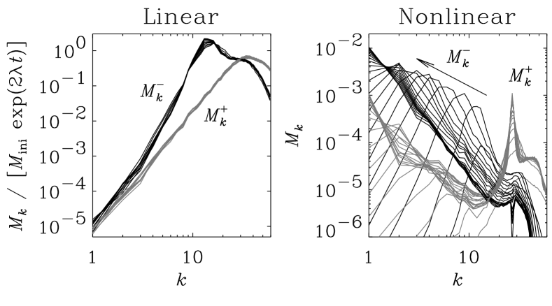
Figure 8.2: Power spectra of magnetic energy of positively and negatively polarized parts ($M_{k}^{+}$ and $M_{k}^{-}$) in the linear and nonlinear regimes. The spectra in the linear regime have been compensated by the exponential growth factor to make them collapse on top of each other. Here the forcing wavenumber is in the dissipative subrange, $k_{\rm f}=27$, but this allows enough scale separation to see the inverse transfer of magnetic energy to smaller $k$. The data are from Run B of Ref. [337].

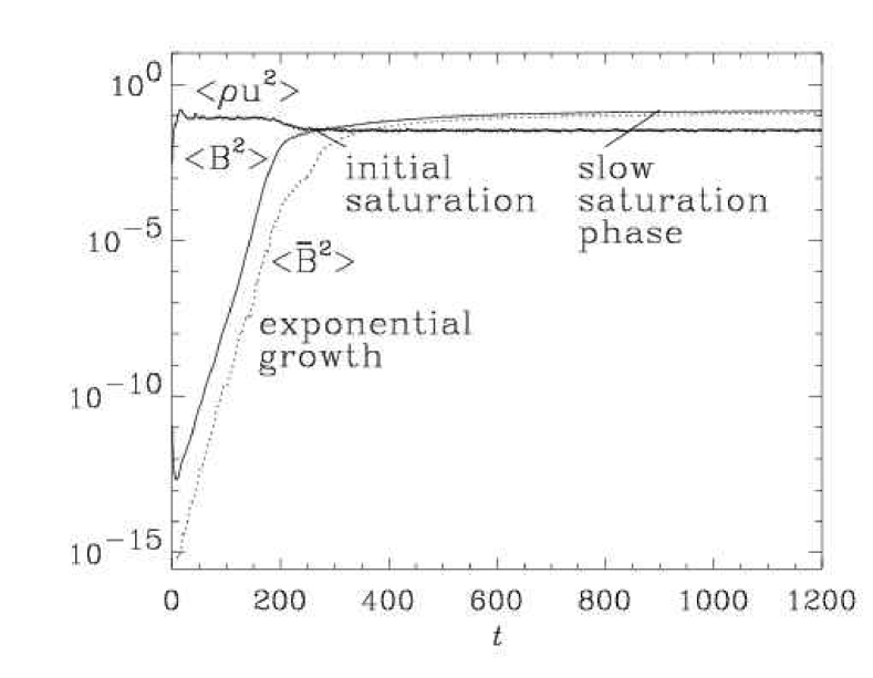
Figure 8.3: The three stages of helical magnetic field growth: exponential growth until initial saturation (when $\langle\bm{B}^{2}\rangle/\mu_{0}=\langle\rho\bm{u}^{2}\rangle$), followed by a (resistively) slow saturation phase. In this plot we have used $\mu_{0}=1$. The energy of the large scale magnetic field, $\langle\overline{\bm{B}}^{2}\rangle$, is shown for comparison. The data are from Run 3 of Ref. [4].

8.4 Emergence of a large scale field

In the simulations of Ref. [4] the flow was forced at an intermediate wavenumber, $k\approx k_{\rm f}=5$, while the smallest wavenumber in the computational domain corresponds to $k=k_{1}=1$. The kinetic energy spectrum peaks at $k\approx k_{\rm f}$, which is therefore also the wavenumber of the energy carrying scale. The turbulence is nearly fully helical with $\langle\bm{\omega}\cdot\bm{u}\rangle/(k_{\rm f}\langle\bm{u}^{2}\rangle)\approx 0.7...0.9$. The initial field is random, but as time goes on it develops a large scale component at wavenumber $k\approx k_{1}=1$; see Fig. 8.4.

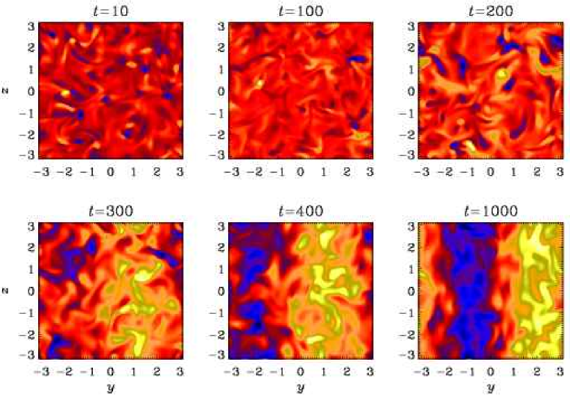
Figure 8.4: Cross-sections of $B_{x}(0,y,z)$ for Run 3 of Ref. [4] at different times showing the gradual build-up of the large scale magnetic field after $t=300$. Dark (light) corresponds to negative (positive) values. Each image is scaled with respect to its min and max values. The final state corresponds to the second eigenfunction given in Eq. (8.4), but with some smaller scale turbulence superimposed.

The large scale field seen in Fig. 8.4 has only one preferred direction, which is the wavevector $\bm{k}_{1}$ of $\overline{\bm{B}}$. Different initial conditions can produce different directions of $\bm{k}_{1}$; see Fig. 6 of Ref. [4]. A suitable definition of the mean field is a two-dimensional average over the two directions perpendicular to $\bm{k}_{1}$. (The most useful choice among the three possibilities can only be taken a posteriori when we know the direction $\bm{k}_{1}$ in which the large scale field varies. So, in practice, one has to calculate all three possibilities and select the right one in the end.) The resulting large scale field is one of the following three eigenfunctions of the curl operator whose wavevectors point along a coordinate direction, i.e.

$$\overline{\bm{B}}(\bm{x})=\pmatrix{\cos k_{\rm m}z\cr\sin k_{\rm m}z\cr 0},\quad\pmatrix{0\cr\cos k_{\rm m}x\cr\sin k_{\rm m}x},\quad\mbox{or}\quad\pmatrix{\sin k_{\rm m}y\cr 0\cr\cos k_{\rm m}y},$$ (8.4)

where $k_{\rm m}=k_{1}=1$. These fields are force-free and are also referred to as Beltrami fields. The large scale field is fully helical, but with opposite (here negative) current helicity relative to the small scale field, i.e. $\overline{\mbox{\boldmath$J$}}\cdot\overline{\bm{B}}=-k_{\rm m}\overline{\bm{B}}^{2}<0$. This property alone allows us to estimate the saturation amplitude of the dynamo, as will be done in the next section.

It is also interesting to note that the one point probability density functions (PDF) of the three magnetic field components are, to a good approximation, gaussian. This is shown in the left hand panel of Fig. 8.5 where we plot one point PDFs of $B_{x}$ and $B_{y}$ for Run 3 of Ref. [4] at the time of saturation. (The PDF of $B_{z}$ looks similar to that of $B_{x}$ and is not shown.)

We recall that, in this particular simulation, the $x$ and $z$ components of the magnetic field show large scale variation in the $y$ direction. One therefore sees two marked humps in the PDFs of $B_{x}$ and $B_{z}$, which can be fitted by a superposition of two gaussians shifted away from zero, together with another gaussian of lower weight around zero. (Note that even though there is a mean $B_{x}$ field, the presence of the random fluctuating component makes the notion of a PDF meaningful. Indeed it is the presence of a mean field that distorts the one point PDF to a double humped form, rather than a gaussian centered at the origin). The $y$ component of the field does not show a large scale field and can be fitted by a single gaussian of the same width. (In the absence of large scale dynamo action the three components of the magnetic field would not be gaussians but stretched exponentials; see Ref. [203] for such results in the context of convection, where there is only small scale dynamo action.) In that case, the modulus of the field (i.e. not its individual components) tends to have a log-normal probability density function. For comparison we show in the right hand panel of Fig. 8.5 the corresponding PDFs for nonhelically forced turbulence.

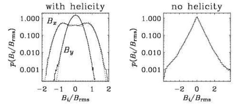
Figure 8.5: Probability density functions of $B_{x}/B_{\rm rms}$ and $B_{y}/B_{\rm rms}$ for Run 3 of Ref. [4] at the time of saturation (left). For comparison, the PDFs are also shown for nonhelically forced turbulence (right). In the left hand plot, the dotted lines give gaussian fits with a width of 0.27. $B_{y}/B_{\rm rms}$ is fitted by a single gaussian around zero, while $B_{x}/B_{\rm rms}$ is fitted by a superposition of three gaussians (one around zero with weight 0.26, and two with weight 0.37 shifted by $\pm 0.76$ away from zero).

8.5 Importance of magnetic helicity

In the following we show that for strongly helical dynamos the saturation amplitude and the saturation time can accurately be estimated from magnetic helicity considerations alone – without actually solving the induction equation explicitly. The argument is similar in nature to the way how the descent speed of a free-falling body can be calculated based on the consideration of kinetic and potential energies alone, without considering the equation of motion. A more accurate treatment of the saturation behavior of helical dynamos will be presented in Sections 9.3 and 9.4.3.

8.5.1 Saturation amplitude

Even though the current helicity of the large and small scale fields are finite, the current helicity of the total (small scale plus large scale) field must approach zero in the long time limit. This is evident from the magnetic helicity equation (3.34) which, for a closed or periodic domain, is simply

$${\mathrm{d}\over\mathrm{d}t}\langle\bm{A}\cdot\bm{B}\rangle=-2\eta\langle\bm{J}\cdot\bm{B}\rangle.$$ (8.5)

Thus, in the steady state ($\mathrm{d}/\mathrm{d}t=0$) one has $\langle\bm{J}\cdot\bm{B}\rangle=0$. However, the time scale on which this can be achieved is the resistive one, as will be discussed in the following.

Splitting the magnetic field and current density into mean and fluctuating components, similar to Eq. (6.4), we have

$$\overline{\bm{J}\cdot\bm{B}}=\overline{\mbox{\boldmath$J$}}\cdot\overline{\bm{B}}+\overline{\bm{j}\cdot\bm{b}},$$ (8.6)

and therefore also $\langle\bm{J}\cdot\bm{B}\rangle=\langle\overline{\mbox{\boldmath$J$}}\cdot\overline{\bm{B}}\rangle+\langle\bm{j}\cdot\bm{b}\rangle$. In the steady state we have

$$-\langle\overline{\mbox{\boldmath$J$}}\cdot\overline{\bm{B}}\rangle=\langle\bm{j}\cdot\bm{b}\rangle\quad\mbox{(steady state)}.$$ (8.7)

Here, overbars denote suitably defined two-dimensional averages (Section 8.4) and angular brackets denote volume averages. The helical forcing tends to produce finite current helicity at small scales. This, in turn, tends to induce finite current helicity of opposite sign at large scales. Depending on the degree of helicity in the forcing, the small scale field will be more or less strongly helical. The degree of helicity of the large scale fields depends also on other factors such as boundary conditions and the presence of shear which produces toroidal field quite independently of helicity.

The case of fractional helicities can be dealt with by introducing efficiency factors [6, 159, 362], but in order to explain the basic point we just assume that both mean and fluctuating fields are fully helical. (This is also likely to be more fully the case when the small scale field arises predominantly due to the tangling of the large scale field by the helical turbulence rather than the small scale dynamo.) So, in the fully helical case we have $\langle\overline{\mbox{\boldmath$J$}}\cdot\overline{\bm{B}}\rangle\approx\mp k_{\rm m}\langle\overline{\bm{B}}^{2}\rangle$ and $\langle\bm{j}\cdot\bm{b}\rangle\approx\pm k_{\rm f}\langle\bm{b}^{2}\rangle$, where $k_{\rm f}$ is the typical wavenumber of the fluctuating field (which is close to the wavenumber of the energy carrying scale). This yields $k_{\rm m}\langle\overline{\bm{B}}^{2}\rangle=k_{\rm f}\langle\bm{b}^{2}\rangle$, and if the small scale field is in equipartition with the turbulent motions, i.e. if $\langle\bm{b}^{2}\rangle\approx\langle\mu_{0}\rho\bm{u}^{2}\rangle\equiv B_{\rm eq}^{2}$, we have [4]

$$\langle\overline{\bm{B}}^{2}\rangle={k_{\rm f}\over k_{\rm m}}\langle\bm{b}^{2}\rangle\approx{k_{\rm f}\over k_{\rm m}}B_{\rm eq}^{2}>B_{\rm eq}^{2}\quad\mbox{(steady state)}.$$ (8.8)

We see that for a fully helical dynamo the large scale field at $k=k_{\rm m}$ is in general in super-equipartition with the kinetic energy of the turbulence. This fact is indeed confirmed by simulations which also show strong large scale fields in super-equipartition; see Fig. 8.6.

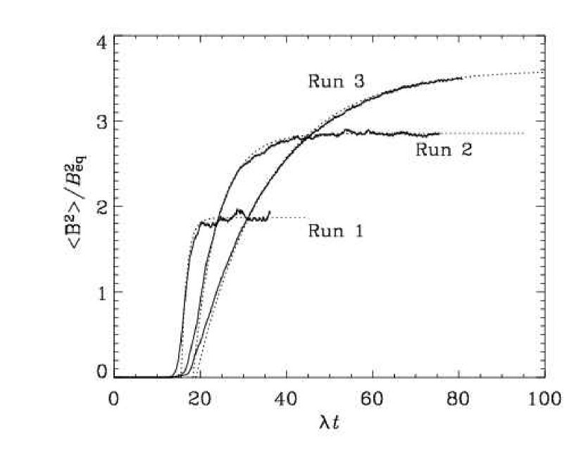
Figure 8.6: Late saturation phase of fully helical turbulent dynamos for three different values of the magnetic Reynolds number: $R_{\rm m}\equiv u_{\rm rms}/\eta k_{\rm f}=2.4$, 6, and 18 for Runs 1, 2, and 3 respectively; see Ref. [4]. The mean magnetic field, $\overline{\bm{B}}$, is normalized with respect to the equipartition value, $B_{\rm eq}=\sqrt{\mu_{0}\rho_{0}}u_{\rm rms}$, and time is normalized with respect to the kinematic growth rate, $\lambda$. The dotted lines represent the formula (8.13) which tracks the simulation results rather well.

Obviously, the simulated values of $\langle\overline{\bm{B}}^{2}\rangle/B_{\rm eq}^{2}$ fall somewhat short of this simplistic estimate, although the estimate becomes more accurate in the case of larger magnetic Reynolds number (Run 3 has ${\rm Re}=R_{\rm m}\equiv u_{\rm rms}/\eta k_{\rm f}\approx 18$, Run 2 has ${\rm Re}=R_{\rm m}\approx 6$, and Run 1 has ${\rm Re}=R_{\rm m}\approx 2.4$).

8.5.2 Saturation time

It turns out that the time dependence in Fig. 8.6 can be well described by a fit formula that can be derived from the magnetic helicity equation. In the following we define the current helicities at large and small scales as

$$C_{1}=\langle\overline{\mbox{\boldmath$J$}}\cdot\overline{\bm{B}}\rangle\quad\mbox{and}\quad C_{\rm f}=\langle\bm{j}\cdot\bm{b}\rangle,$$ (8.9)

respectively, and the magnetic helicities at large and small scales as

$$H_{1}=\langle\overline{\mbox{\boldmath$A$}}\cdot\overline{\bm{B}}\rangle\quad\mbox{and}\quad H_{\rm f}=\langle\bm{a}\cdot\bm{b}\rangle,$$ (8.10)

respectively. Near saturation we have $|C_{1}|\approx|C_{\rm f}|$, but because $C_{1}=k_{1}^{2}H_{1}$ and $C_{\rm f}=k_{\rm f}^{2}H_{\rm f}$ together with $k_{1}/k_{\rm f}\ll 1$, we have

$$|H_{1}|\gg|H_{\rm f}|\quad\mbox{(near saturation)}.$$ (8.11)

Furthermore, as will be shown more convincingly in Section 9.4.2, the small scale field tends to saturate on a dynamical time scale. At late times we can therefore, to a good approximation, neglect the time derivative of $H_{\rm f}$ relative to the time derivative of $H_{1}$ in Eq. (8.5), so

$$\dot{H}_{1}=-2\eta k_{1}^{2}H_{1}-2\eta k_{\rm f}^{2}H_{\rm f}.$$ (8.12)

Solving Eq. (8.12) for $H_{1}(t)$, using a given value of $H_{\rm f}=\mbox{const}$, we find

$$H_{1}(t)=H_{\rm f}{k_{\rm f}^{2}\over k_{1}^{2}}\left[1-\e^{-2\eta k_{1}^{2}(t-t_{\rm sat})}\right].$$ (8.13)

The time $t_{\rm sat}$ is determined by the strength of the initial seed magnetic field, $B_{\rm ini}$; for weaker fields it takes somewhat longer to reach saturation. Since the growth is exponential, the dependence is only logarithmic, so $t_{\rm sat}=\lambda^{-1}\ln(B_{\rm eq}/B_{\rm ini})$, where $\lambda$ is the growth rate of the rms field strength of the total field. Equation (8.13) describes the evolution of $\overline{\bm{B}}$ quite well, as is shown in Fig. 8.6.

Clearly, Eq. (8.13) is not applicable too close to $t=t_{\rm sat}$. This is also evident from Fig. 8.6, which shows that in the simulations (solid lines) there is a finite mean field already at $t=t_{\rm sat}$. In order to describe this phase correctly, one has to retain the time derivative of $H_{\rm f}$, as will be done in Sections 9.3 and 9.4 in the framework of the dynamical quenching model. At early times resistive effects have not yet played a role, so the total magnetic helicity must be approximately zero, and this means that a helical large scale field must be smaller than $B_{\rm eq}$; see Section 9.4.2 for details.

8.6 Alpha effect versus inverse cascade

The process outlined above can be interpreted in two different ways: inverse cascade of magnetic helicity and/or $\alpha$ effect. The two are similar in that they tend to produce magnetic energy at scales larger than the energy-carrying scale of the turbulence. As can be seen from Figs. 8.1 and 8.2, the present simulations support the notion of nonlocal inverse transfer [4]. However, this is not really an inverse cascade in the usual sense, because there is no sustained flux of energy through wavenumber space, as in the direct Kolmogorov cascade. Instead, there is just a bump traveling in wavenumber space from a $k$ that is already smaller than $k_{\rm f}$ to even smaller values of $k$. In that respect, the present simulations seem to differ from the interpretation of PFL based on the EDQNM closure approximation [304].

The other interpretation is in terms of the $\alpha$ effect. We recall that for $\alpha^{2}$ dynamos there is a wavenumber $k_{\max}$ where the growth of the large scale field is fastest; see Section 6.5.1. For reasonable estimates, $k_{\max}$ coincides with the position of the secondary bump in the spectrum; see Ref. [4], Sect. 3.5. This can be taken as evidence in favor of the $\alpha$ effect. In the nonlinear regime, the secondary bump travels to the left in the spectrum (i.e. toward smaller $k$). In the EDQNM picture this has to do with the equilibration of kinetic and current helicities at progressively smaller wavenumbers, which then leads to saturation at that wavenumber, but permits further growth at smaller wavenumbers until equilibration occurs, and so forth. Another interpretation is simply that, after $\alpha$ is quenched to a smaller value, the magnetic spectrum now peaks at $k_{\max}=\alpha/(2\eta_{\rm T})$, which is now also smaller. At this lower wavenumber the spectrum is still not fully saturated; the field continues to grow here until equilibration is attained also at that scale.

8.7 Nonlinear $\alpha$ effect

It is quite clear that $\alpha$ must somehow depend on the strength of the mean field, $\overline{\bm{B}}$. By considering the effect of $\overline{\bm{B}}$ on the correlation tensor of the turbulence it has been possible to derive a correction to $\alpha$ of the form [329, 372, 373]

$$\alpha=\alpha_{\rm K}\left(1-\overline{\bm{B}}^{2}/B_{\rm eq}^{2}\right)\quad\mbox{(for $|\overline{\bm{B}}|\ll B_{\rm eq}$)}.$$ (8.14)

For practical applications, to make sure that $|\alpha|$ decreases with increasing field strength and to prevent $\alpha$ from changing sign, Eq. (8.14) is often replaced by the fit formula [374]

$$\alpha={\alpha_{\rm K}\over 1+\overline{\bm{B}}^{2}/B_{\rm eq}^{2}}\quad\mbox{(conventional quenching)}.$$ (8.15)

It should also be noted that fully nonlinear expressions exist; see, e.g., Ref. [310]. However, it has long been noted that in the astrophysically relevant case, $R_{\rm m}\gg 1$, the magnitude of the fluctuating field is likely to exceed that of the mean field, i.e. $\bm{b}^{2}/\overline{\bm{B}}^{2}\gg 1$. Indeed, a naive application of kinematic mean field theory suggests that [301, 375, 376]

$$\langle\bm{b}^{2}\rangle/\langle\overline{\bm{B}}^{2}\rangle=R_{\rm m}\quad\mbox{(kinematic theory)}.$$ (8.16)

This result is a direct consequence of flux freezing (Section 3.3) during the compression of a uniform field of strength $\overline{B}$ and scale $L$ into a sheet of ‘skin’ thickness $d=LR_{\rm m}^{1/2}$. It can also be derived under more general assumptions, but then only in the two-dimensional case [377]; see Appendix C. Further in the three dimensional case, the small scale field dynamo can also generate $\bm{b}$ at a rate much faster than $\overline{\bm{B}}$, and unrelated to the strength of the mean field [378].

Nevertheless, the above argument has been used to suggest that the quenching formula (8.15) should take the small scale field, obeying the relation in Eq. (8.16), into account. Using Eq. (8.16), this then leads to

$$\alpha={\alpha_{\rm K}\over 1+R_{\rm m}\overline{\bm{B}}^{2}/B_{\rm eq}^{2}}\quad\mbox{(catastrophic quenching)}.$$ (8.17)

This formula was first suggested by Vainshtein and Cattaneo [340]. Only recently it has become clear that, even though Eq. (8.16) is actually no longer valid in the nonlinear regime, Eq. (8.17) can indeed emerge in a more rigorous analysis under certain circumstances [6].

The problem with Eq. (8.17) is that $\alpha$ becomes strongly suppressed already for $\overline{\bm{B}}^{2}/B_{\rm eq}^{2}\ll 1$. Conversely, for the sun where $\overline{\bm{B}}^{2}/B_{\rm eq}^{2}\approx 1$, this means that $\alpha$ would be negligibly small. Equation (8.17) is therefore sometimes referred to as catastrophic quenching formula.

Given the potentially catastrophic outcome of mean field theory when applying Eq. (8.17) to astrophysically relevant situations, the problem of $\alpha$ quenching has begun to attract significant attention in the last few years. Considerable progress has recently been made by restricting attention to the simplest possible system that still displays an $\alpha$ effect, but that is otherwise fully nonlinear.

8.8 Determining alpha quenching from isotropic box simulations

The issue of (catastrophic) $\alpha$ quenching was preceded by the related issue of $\eta_{\rm t}$ quenching. Indeed, already 30 years ago concerns have been expressed [379] that turbulent diffusion might not work when the magnitude of the field is strong. A serious argument against catastrophic $\eta_{\rm t}$ quenching came from the measurements of decay times of sunspots where the magnetic field is strong and yet able to decay almost on a dynamical time scale. Estimates for the turbulent magnetic diffusivity in sunspots suggest $\eta_{\rm t}\approx 10^{11}\,{\rm cm}^{2}\,{\rm s}^{-1}$ [380, 381, 382, 383].

Quantitatively, catastrophic (i.e. $R_{\rm m}$-dependent) $\eta_{\rm t}$ quenching was first suggested based on two-dimensional simulations with an initially sinusoidally modulated large scale magnetic field in the plane of the motions [384]. However, these results have to be taken with caution, because constraining the field to be in the plane of the motions is artificial in that the interchange of field lines is then impossible. Field lines that undergo interchanging motions can remain nearly straight, so not much work is involved and one would therefore not necessarily expect catastrophic quenching if the flow were allowed to be fully three-dimensional. This has been confirmed using both closure models [302] and three-dimensional simulations [385]. Nevertheless, the possibility of catastrophic quenching of $\eta_{\rm t}$ is not completely ruled out. Simulations are not yet conclusive, as discussed below in Section 9.4.3. However, unlike the case of catastrophic $\alpha$ quenching, which can be explained as a consequence of magnetic helicity conservation, there is no similar argument for an $R_{\rm m}$ dependent quenching of $\eta_{\rm t}$.

The issue of catastrophic $\alpha$ quenching was originally motivated by analogy with catastrophic $\eta_{\rm t}$ quenching in two dimensions [340], but then backed up by simulations with an imposed field [311], so $\alpha$ is calculated as the ratio of the resulting electromotive force and the imposed magnetic field; cf. Section 6.4. Another technique to measure $\alpha$ is to modify or remove a component of the mean field in an otherwise self-consistent simulation and to describe the response of the system in terms of $\alpha$ effect and turbulent diffusion [4]. This technique is easily explained by looking, for example, at the $x$-component of the $\alpha^{2}$ dynamo equation (Section 6.5.1),

$${\partial\overline{B}_{x}\over\partial t}=-\alpha{\partial\overline{B}_{y}\over\partial z}+(\eta+\eta_{\rm t}){\partial^{2}\overline{B}_{x}\over\partial z^{2}}.$$ (8.18)

If, at some point in time, the $x$ component of the mean field is removed, i.e. $B_{x}\to B_{x}-\overline{B}_{x}$, then Eq. (8.18) describes the immediate recovery of $\overline{B}_{x}$. The recovery is described by the first term on the rhs of Eq. (8.18), and the rate of recovery is proportional to $\alpha$. This method allows an estimate not only of $\alpha$, but also of $\eta_{\rm t}$ by measuring the simultaneous temporary reduction of $\overline{B}_{y}$. It turns out [4] that both methods give comparable results and confirm the catastrophic quenching results (8.17). This result will later be understood as a special case of the dynamical quenching formula in the nearly steady limit for fully force-free (force-free) fields; see Eq. (9.19).

Yet another method is to impose a nonuniform field that is a solution of the mean field dynamo equations – for example a Beltrami field in the case of periodic box. By changing the wavelength of the Beltrami field, one can determine both $\alpha$ and $\eta_{\rm t}$ simultaneously. This method has been used in connection with the underlying flow field of the Karlsruhe dynamo experiment [219, 218].

8.9 Dynamo waves in simulations with shear

The fact that dynamos exhibit cyclic behavior when there is shear is not surprising if one recalls the type of solutions that are possible for $\alpha\Omega$ dynamos (Section 6.5.2). On the other hand, until only a few years ago the concept of mean field theory was only poorly tested and there was enough reason to doubt its validity especially in the nonlinear regime. Even in the linear regime the relevance of mean field theory has been doubtful because the mean field can be much weaker than the fluctuating field [143, 339].

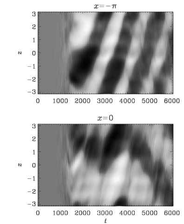
Figure 8.7: Space-time diagram of the mean toroidal field at $x=-\pi$ (negative local shear) and $x=0$ (positive local shear). Dark (light) shadings refer to negative (positive) values. Note the presence of dynamo waves traveling in the positive (negative) $z$-direction for negative (positive) local shear (from Ref. [386]).

Given all these reservations about the credibility of mean field theory it was a surprise to see that cyclic dynamo action does actually work [386]. As in the simulations without shear, the emergence of a large scale field is best seen in the nonlinear regime; see Fig. 8.7. The reason is that prior to saturation several different modes may be excited, while in the nonlinear regime most of the modes are suppressed by the most dominant mode. Nonlinearity therefore has a ‘self-cleaning’ effect [4, 286].

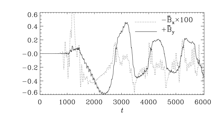
Figure 8.8: Evolution of $\overline{B}_{x}$ and $\overline{B}_{y}$ at $x=-\pi$ and $z=0$. Note that $\overline{B}_{x}$ has been scaled by a factor $-100$. Here the overbars denote only a one-dimensional average over the direction of shear, $y$. (Adapted from Ref. [386].)

The dynamo exhibits a certain phase relation between poloidal and toroidal fields (see Fig. 8.8). This phase relation is quite similar to what is expected from a corresponding mean field model (see Section 6.5.3). Comparison with $\alpha$ quenching models in the same geometry (see Fig. 9 of Ref. [386]) produces similarly anharmonic oscillations, as seen in Fig. 8.8. This strongly suggests that the simulation results can basically be described in terms of the mean field concept.

An important question for astrophysical applications is which of the properties of the dynamo depend on resistivity. Certainly the late saturation behavior of the field does depend on resistivity and satisfies the ‘magnetic helicity constraint’ embodied by Eq. (8.13); see Fig. 8 of Ref. [386]. Subsequent simulations for different values of the magnetic Reynolds number also seem to confirm that the cycle frequency, $\omega_{\rm cyc}$, scales resistively and that $\omega_{\rm cyc}/(\eta k_{1}^{2})\approx{\rm const}{}={\cal O}(10)$ for $u_{\rm rms}/(\eta k_{1})$ ranging from 30 to 200; see Table 5 of Ref. [159]. On the other hand, in all cases the large scale magnetic energy exceeds the kinetic energy by a factor that is between 20 (for smaller $R_{\rm m}$) and 60 (for larger $R_{\rm m}$). It is therefore clear that these models are in a very different parameter regime than the solar dynamo where the energy of the mean field is at most comparable to the kinetic energy of the turbulence. Furthermore, all turbulent transport coefficients are necessarily strongly suppressed by such strong fields even if the actual suppression is not explicitly dependent on the magnetic Reynolds number. A more detailed interpretation of these simulation data has been possible by using a dynamical quenching model that will be discussed in Section 9.4.3.

8.10 The magnetic helicity constraint in a closure model

The magnetic helicity constraint is quite general and independent of any mean field or other model assumptions. All that matters is that the flow possesses kinetic helicity. The generality of the magnetic helicity constraint allows one to eliminate models that are incompatible with magnetic helicity conservation. In previous sections we discussed a simple unified model of large and small scale dynamo, generalizing the Kazantsev model to include helical velocity correlations. In [236, 257] this model was further extended to include ambipolar diffusion as a model nonlinearity. This is a useful toy model since the magnetic field still obeys helicity conservation even after adding ambipolar drift. So it is interesting to see how in this model the $\alpha$ effect is being regulated by the change in magnetic helicity, and whether there are similarities to the dynamical quenching model under full MHD.

This issue was examined in Ref. [286] by solving the moment equations derived in [236, 257] numerically. We have given in the Appendix A the derivation of the moment equations for the magnetic correlations in the presence of ambipolar drift. In deriving the moment equations with ambipolar drift nonlinearity, one encounters again a closure problem. The equations for the second moment, fortunately, contains only a fourth order correlator of the magnetic field. This was closed in [236, 257] assuming that the fourth moment can be written as a product of second moments. The equations for the longitudinal correlation function $M_{\rm L}(r,t)$ and the correlation function for magnetic helicity density, $H(r,t)$, then are the same as Eqs. (5.28) and (5.29), except for additions to the coefficients $\eta_{T}(r)$ and $\alpha(r)$. We have

$${\partial M_{\rm L}\over\partial t}={2\over r^{4}}{\partial\over\partial r}\left(r^{4}\eta_{\rm N}(r){\partial M_{\rm L}\over\partial r}\right)+GM_{\rm L}+4\alpha_{\rm N}(r)C,$$ (8.19)

$${\partial H\over\partial t}=-2\eta_{\rm N}C+\alpha_{\rm N}M_{\rm L},$$ (8.20)

where

$$\alpha_{\rm N}=\alpha(r)+4aC(0,t),\quad\eta_{\rm N}=\eta_{T}(r)+2aM(0,t).$$ (8.21)

Note that at large scales

$$\alpha_{\infty}\equiv\alpha_{\rm N}(r\rightarrow\infty)=-{\textstyle{1\over 3}}\tau\langle\bm{\omega}\cdot\bm{u}\rangle+{\textstyle{1\over 3}}\tau_{\rm AD}\langle\bm{J}\cdot\bm{B}\rangle/\rho_{0},$$ (8.22)

$$\eta_{\infty}\equiv\eta_{\rm N}(r\rightarrow\infty)={\textstyle{1\over 3}}\tau\langle\bm{u}^{2}\rangle+{\textstyle{1\over 3}}\tau_{\rm AD}\langle\bm{B}^{2}\rangle/\mu_{0}\rho_{0},$$ (8.23)

where $\tau_{\rm AD}=2a\rho_{0}$. Here, angular brackets denote volume averages over all space. This makes sense because the system is homogeneous. Expression (8.22) for $\alpha_{\infty}$ is very similar to the $\alpha$ suppression formula due to the current helicity contribution first found in the EDQNM treatment by [304] (see Section 7.2). The expression for $\eta_{\infty}$ has the nonlinear addition due to ambipolar diffusion. It is important to point out that the closure model, even including the above nonlinear modifications, explicitly satisfies helicity conservation. This can be seen by taking $r\to 0$ in (8.20). We get

$$\dot{H}(0,t)=-2\eta C(0,t),\quad\mathrm{d}\langle\bm{A}\cdot\bm{B}\rangle/\mathrm{d}t=-2\eta\langle\bm{J}\cdot\bm{B}\rangle,$$ (8.24)

where we have used the fact that $\langle\bm{A}\cdot\bm{B}\rangle=6H(0,t)$, and $\langle\bm{J}\cdot\bm{B}\rangle=6C(0,t)$. It is this fact that makes it such a useful toy model for full MHD (see below).

Adopting functional forms of $T_{\rm L}(r)$ and $F(r)$ constructed from the energy and helicity spectra resembling Run 3 of Ref. [4], Eqs. (8.19) and (8.20) were solved numerically [286]. In the absence of kinetic helicity, $F=0$, and without nonlinearity, $a=0$, the standard small scale dynamo solutions are recovered. The critical magnetic Reynolds number based on the forcing scale is around 60 (here we have not converted the scale into a wavenumber). In the presence of kinetic helicity this critical Reynolds number decreases, confirming the general result that kinetic helicity promotes dynamo action [257, 287]. In the presence of nonlinearity the exponential growth of the magnetic field terminates when the magnetic energy becomes large. After that point the magnetic energy continues however to increase nearly linearly. Unlike the case of the periodic box the magnetic field can here extend to larger and larger scales; see Fig. 8.9. The corresponding magnetic energy spectra,

$$E_{\rm M}(k,t)={1\over\pi}\int_{0}^{L}\,(kr)^{3}M_{\rm L}(r,t)\,j_{1}(kr)\,\mathrm{d}k,$$ (8.25)

are shown in Fig. 8.10.

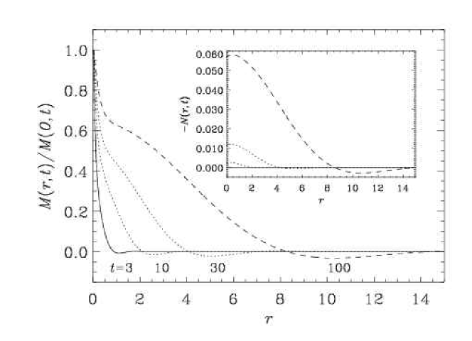
Figure 8.9: Evolution of magnetic correlation function $M_{L}$ (denoted by $M(r,t)$ in this figure) for different times, for $\eta=10^{-3}$. The correlation function of the magnetic helicity (denoted in this figure by $N(r,t)$), is shown in the inset. $\eta=10^{-3}$.

Figure 8.10: Evolution of magnetic energy spectra. Note the propagation of magnetic helicity and energy to progressively larger scales. The $k^{-2}$ slope is given for orientation. Note the similarities with Figs. 7.1 and 8.2.

The resulting magnetic field is strongly helical and the magnetic helicity spectra (not shown) satisfy $|H_{\rm M}(k,t)|\mathrel{\mathchoice{\vbox{\offinterlineskip\halign{\hfil$\displaystyle#$\hfil\cr<\cr\sim\cr}}}{\vbox{\offinterlineskip\halign{\hfil$\textstyle#$\hfil\cr<\cr\sim\cr}}}{\vbox{\offinterlineskip\halign{\hfil$\scriptstyle#$\hfil\cr<\cr\sim\cr}}}{\vbox{\offinterlineskip\halign{\hfil$\scriptscriptstyle#$\hfil\cr<\cr\sim\cr}}}}(2/k)E_{\rm M}(k,t)$. One sees in Fig. 8.10 the development of a helicity wave traveling toward smaller and smaller $k$. This is just as in the EDQNM closure model [304] (see Fig. 7.1) and in the simulations of the full MHD equations [4, 300] (see Fig. 8.2).

Figure 8.11: (a) Evolution of $\langle\bm{J}\cdot\bm{B}\rangle$ for different values of $\eta$. The corresponding value of $\alpha_{\infty}$ is shown on the right hand side of the plot. (b) The evolution of magnetic energy for the same values of $\eta$.

In the following we address the question of whether or not the growth of this large scale field depends on the magnetic Reynolds number (as in [4]). To a good approximation the wavenumber of the peak is given by

$$k_{\rm peak}(t)\approx\alpha_{\infty}(t)/\eta_{\infty}(t).$$ (8.26)

This result is familiar from mean field dynamo theory (see also Ref. [257]), where the marginal state with zero growth rate, has $k=\alpha/\eta_{t}$, while the fastest growing mode has $k=\alpha/2\eta_{t}$; see Section 6.5.1. In our model problem, the large scale field, seems to go to a quasi-static state (which has no $1/2$ factor) rather than the fastest growing mode, and then evolve slowly (on the resistive time scale), through a sequence of such states. This evolution to smaller and smaller wavenumbers is also consistent with simulations ([4], Sect. 3.5). Note that here $k_{\rm peak}$ decreases with time because $\alpha_{\infty}$ tends to a finite limit and $\eta_{\infty}$ increases; see Section 6.5.1. (This is not the case in the box calculations where $k_{\rm peak}\geq 2\pi/L$.)

As we saw from Eq. (8.24) the magnetic helicity, $\langle\bm{A}\cdot\bm{B}\rangle=6\,H(0,t)$, can only change if there is microscopic magnetic diffusion and finite current helicity, $\langle\bm{J}\cdot\bm{B}\rangle=6\,C(0,t)$. In Fig. 8.11 we show that, after some time $t=t_{\rm s}$, the current helicity $\langle\bm{J}\cdot\bm{B}\rangle$ reaches a finite value. This value increases somewhat as $\eta$ is decreased. In all cases, however, $\tau_{\rm AD}\langle\bm{J}\cdot\bm{B}\rangle/\rho_{0}$ stays below $\tau\langle\bm{\omega}\cdot\bm{u}\rangle$, so that $|\alpha_{\infty}|$ remains finite; see (8.22). A constant $\langle\bm{J}\cdot\bm{B}\rangle$ implies from (8.24) that $\langle\bm{A}\cdot\bm{B}\rangle$ grows linearly at a rate proportional to $\eta$. However, since the large scale field is helical, and since most of the magnetic energy is by now (after $t=t_{\rm s}$) in the large scales, the magnetic energy is proportional to $\langle\bm{B}^{2}\rangle\approx k_{\rm peak}\langle\bm{A}\cdot\bm{B}\rangle$, and can therefore only continue to grow at a resistively limited rate, see Fig. 8.11. It is to be emphasized that this explanation is analogous to that given in Ref. [4] and Section 8.3 for the full MHD case; the helicity constraint is independent of the nature of the feedback!

These results show that ambipolar diffusion (AD) provides a useful model for nonlinearity, enabling analytic (or semi-analytic) progress to be made in understanding nonlinear dynamos. There are two key features that are shared both by this model and by the full MHD equations: (i) large scale fields are the result of a nonlocal inverse cascade as described by the $\alpha$ effect, and (ii) after some initial saturation phase the large scale field continues to grow at a rate limited by magnetic diffusion. This model also illustrates that it is helicity conservation that is at the heart of the nonlinear behavior of large scale dynamos; qualitatively similar restrictions arise even for very different nonlinear feedback provided the feedback obeys helicity conservation.

8.11 Nonhelical large scale turbulent dynamos with shear

Much of the discussion on large scale dynamos has focused on the $\alpha$ effect. In recent years attention has been drawn to the possibility of producing large scale fields by other effects such as the shear–current or $\overline{\mbox{\boldmath$W$}}\times\overline{\mbox{\boldmath$J$}}$ effect [322, 323, 324]. As remarked in Section 6.6 (where this new term was denoted by $\bm{\delta}$) this effect is related to Rädler’s [328] $\bm{\Omega}\times\overline{\mbox{\boldmath$J$}}$ effect in that it has the same functional form. At least two more possibilities have been offered for explaining large scale fields in shearing environments without invoking kinetic helicity. One is the incoherent $\alpha$ effect [387] and the other one is the Vishniac and Cho flux [388]. Both effects are related to the $\alpha$ effect, but there is no kinetic helicity, so there can only be helicity fluctuations (former case) or there can be a magnetic contribution to the $\alpha$ effect (latter case).

In simulations of realistic systems it is easily possible that a number of effects operate simultaneously, so one cannot be sure that the $\alpha$ effect is not also contributing. This is different in systems where turbulence and shear are driven by body forces such as those discussed in Section 8.9.

Figure 8.12: Evolution of the energies of the total field $\langle\bm{B}^{2}\rangle$ and of the mean field $\langle\overline{\bm{B}}^{2}\rangle$, in units of $B_{\rm eq}^{2}$, for runs with non-helical forcing and open or closed boundaries; see the solid and dotted lines, respectively. The inset shows a comparison of the ratio $\langle\overline{\bm{B}}^{2}\rangle/\langle\bm{B}^{2}\rangle$ for nonhelical ($\alpha=0$) and helical ($\alpha>0$) runs. For the nonhelical case the run with closed boundaries is also shown (dotted line near $\langle\overline{\bm{B}}^{2}\rangle/\langle\bm{B}^{2}\rangle\approx 0.07$). Note that saturation of the large scale field occurs on a dynamical time scale; the resistive time scale is given on the upper abscissa. Adapted from Ref. [55].

Meanwhile, using a modified toroidal shear profile of the form [389]

$$\overline{\mbox{\boldmath$U$}}\approx(0,\cos k_{1}x\cos k_{1}z,0),$$ (8.27)

it has been possible to produce strong mean fields [55, 390]. Here, mean fields are defined as toroidal averages. In Fig. 8.12 we show the evolution of the normalized magnetic energy of the total field $\langle\bm{B}^{2}\rangle/B_{\rm eq}^{2}$, and of the mean field $\langle\overline{\bm{B}}^{2}\rangle/B_{\rm eq}^{2}$. Both components increase first exponentially until saturation sets in. However, the ratio between the two, $\langle\overline{\bm{B}}^{2}\rangle/\langle\bm{B}^{2}\rangle$, which is shown in the inset of Fig. 8.12, is rather small ($\approx 0.07$) during the early kinematic phase, but then it increases to values of around 0.7. In the inset, comparison is made with the case where the turbulence is driven with negative kinetic helicity, giving rise to a positive $\alpha$ effect (the graph is therefore denoted by “$\alpha>0$”). It turns out that in both cases (with and without helicity) the energy in the mean field is comparable

A more dramatic difference is seen in the case of closed (perfectly conducting) outer boundaries. Although the initial exponential increase is almost equally fast, the field now saturates at a much lower level and it completely lacks a mean field, i.e. $\langle\overline{\bm{B}}^{2}\rangle/\langle\bm{B}^{2}\rangle\approx 0.07$ even during the saturated state. This is a striking demonstration of the importance of allowing for magnetic helicity fluxes out of the domain. It is important that, due to the presence of shear, such fluxes can already be driven inside the domain by the Vishniac and Cho flux, as was demonstrated earlier [389, 391]. Without internal helicity transport, e.g. in the absence of shear, open boundaries alone are not sufficient to alleviate the magnetic helicity constraint [392]. We return to this issue in Section 9.6.

9 Magnetic helicity in mean field models

9.1 General remarks

We have seen from both numerical simulations and closure models that magnetic helicity conservation strongly constrains the evolution of large scale fields. Due to helicity conservation, large scale fields are able to grow eventually only on the resistive time scale. Note that the magnetic helicity evolution does not explicitly depend on the nonlinear backreaction due to the Lorentz force. It merely depends on the induction equation. It therefore provides a strong constraint on the nonlinear evolution of the large scale field. The effects of this constraint need to be incorporated into any treatment of mean field dynamos. This will be the aim of the present section, where we solve simultaneously the mean field dynamo equation (with the turbulent coefficients determined by the nonlinear backreaction) together with helicity conservation equations.

We will see that the magnetic helicity conservation equations for the mean and the turbulent fields, as well as of course the mean field dynamo equation, involve understanding the mean turbulent EMF, $\overline{\mbox{\boldmath${\mathcal{E}}$}}{}$, in the nonlinear regime. So we will need to model the nonlinear effects on $\overline{\mbox{\boldmath${\mathcal{E}}$}}{}$, taking into account nonlinear backreaction effects of the Lorentz force due to both mean and fluctuating fields.

There are two quite different forms of feedback that can arise. One is the effect of the dynamo-generated mean field on the correlation tensor of the turbulence, $\overline{u_{i}u_{j}}$. The growing mean field could cause the suppression of the $\alpha$ effect and turbulent diffusion. Such modifications of the turbulent transport coefficients have been calculated since the early seventies [372, 373], adopting usually an approximation (random waves or FOSA), which linearizes the relevant equations in the fluctuations. This approach missed an important additional ingredient in the nonlinear backreaction due to Lorentz forces: modifications to $\overline{\mbox{\boldmath${\mathcal{E}}$}}{}$ that involve the fluctuating fields themselves. These arise in calculating $\overline{\bm{u}\times\bm{b}}$ from terms involving the correlation of $\bm{b}$ and the Lorentz force in the momentum equation (see below). In particular, the $\alpha$ effect gets renormalized in the nonlinear regime by the addition of a term proportional to the current helicity of the fluctuating field. This is an important effect which is crucial for the correct description of the dynamo saturation, but one which has been missed in much of the earlier work. The renormalization of the $\alpha$ effect is quite general and can occur even when the large scale dynamo effect does not involve an $\alpha$ effect in the kinematic regime. Examples are the $\bm{\Omega}\times\overline{\mbox{\boldmath$J$}}$ and $\overline{\mbox{\boldmath$W$}}\times\overline{\mbox{\boldmath$J$}}$ (or shear current) effects discussed in Section 6.6.

The full problem of solving the induction equation and the momentum (Navier-Stokes) equation including the Lorentz force simultaneously, is a formidable one. One either takes recourse to numerical simulations or uses rather more uncertain analytic approximations in numerical mean field models. The analytic treatments of the backreaction typically involve the quasi-linear approximation or a closure scheme to derive corrections to the mean field dynamo coefficients. For example the EDQNM closure suggests that the $\alpha$ effect is renormalized by the addition a term proportional to the current helicity of the small scale field $\overline{\bm{j}\cdot\bm{b}}$, while the turbulent diffusion is left unchanged. It would be useful to understand this result in a simpler context. For this purpose it can be illuminating to examine a simple heuristic treatment of the effects of the backreaction. However, since such a treatment is not rigorous, we defer the discussion to Appendix D and move straight to the more convincing derivation in terms of the minimal tau approximation.

9.2 The minimal tau approximation: nonlinear effects

In this section we discuss the main aspects of the minimal tau approximation (MTA). Again, for the purpose of clarity, we restrict ourselves to the assumption of isotropy [8, 316, 321], but the method can readily be and has been applied to the anisotropic case [320, 393]. A full treatment of inhomogeneous and anisotropic turbulence is given in Section 10.

In order to incorporate the evolution equations for the fluctuating parts in the expression for $\overline{\mbox{\boldmath${\mathcal{E}}$}}{}$ one can just calculate its time derivative, rather than calculating $\overline{\mbox{\boldmath${\mathcal{E}}$}}{}$ itself [8]. This way one avoids the approximate integration in Eqs. (6.19) and (6.20). Thus, one calculates

$${\partial\overline{\mbox{\boldmath${\mathcal{E}}$}}{}\over\partial t}=\overline{\dot{\bm{u}}\times\bm{b}}+\overline{\bm{u}\times\dot{\bm{b}}},$$ (9.1)

where dots denote partial differentiation with respect to $t$. The dominant contributions in these two terms are (using $\rho_{0}=\mu_{0}=1$)

$$\overline{\dot{\bm{u}}\times\bm{b}}={\textstyle{1\over 3}}\overline{\bm{j}\cdot\bm{b}}\;\overline{\bm{B}}+\overline{(\bm{j}\times\bm{b})\times\bm{b}}-\overline{(\bm{\omega}\times\bm{u})\times\bm{b}}-\overline{\bm{\nabla}p\times\bm{b}}+\ldots,$$ (9.2)

$$\overline{\bm{u}\times\dot{\bm{b}}}=-{\textstyle{1\over 3}}\overline{\bm{\omega}\cdot\bm{u}}\;\;\overline{\bm{B}}-{\textstyle{1\over 3}}\overline{\bm{u}^{2}}\;\;\overline{\mbox{\boldmath$J$}}+\overline{\bm{u}\times\bm{\nabla}\times(\bm{u}\times\bm{b})}+\ldots,$$ (9.3)

where the first term on the right hand side of Eq. (9.2) and the first two terms on the right hand side of Eq. (9.3) are the usual quadratic correlation terms; all other terms are triple correlations. (For a detailed derivation see Section 10 below.) Thus, we can write

$${\partial\overline{\mbox{\boldmath${\mathcal{E}}$}}{}\over\partial t}=\tilde{\alpha}\overline{\bm{B}}-\tilde{\eta}_{\rm t}\overline{\mbox{\boldmath$J$}}+\overline{\bm{T}},$$ (9.4)

where $\overline{\bm{T}}$ are the triple correlation terms, and

$$\tilde{\alpha}=-{\textstyle{1\over 3}}\left(\overline{\bm{\omega}\cdot\bm{u}}-\overline{\bm{j}\cdot\bm{b}}\right),\quad\mbox{and}\quad\tilde{\eta}_{\rm t}={\textstyle{1\over 3}}\overline{\bm{u}^{2}},$$ (9.5)

are turbulent transport coefficients that are related to $\alpha$ and $\eta_{\rm t}$, as used in Eq. (6.18), via $\alpha=\tau\tilde{\alpha}$ and $\eta_{\rm t}=\tau\tilde{\eta}_{\rm t}$. Note that, at this level of approximation, there are no free parameters in the expression for $\tilde{\alpha}$, neither in front of $\overline{\bm{\omega}\cdot\bm{u}}$ nor in front of $\overline{\bm{j}\cdot\bm{b}}$. However, for strong magnetic fields, there could be quenching functions, $g_{\rm K}(\overline{\bm{B}})$ and $g_{\rm M}(\overline{\bm{B}})$, in front of both terms [394]. We should also point out that in the above derivation, $\bm{u}$ and $\bm{b}$ refer to the actual small scale velocity and magnetic fields, and not to any perturbed field. (This could also include any ‘nonhelical’ SSD generated $\bm{b}$, although we see that this does not renormalize $\eta_{\rm t}$ and may not contribute to the current helicity term at leading order.) The full derivation for the more general case of slow rotation, weak stratification and for general magnetic and kinetic spectra (possibly with a $k$-dependent $\tau$), is given the Section 10.

As we have already emphasized earlier, the crucial step is that now, unlike the case of FOSA or the heuristic treatment, the triple correlators are not neglected, but their sum is assumed to be a negative multiple of the second order correlator, i.e. $\overline{\bm{T}}=-\overline{\mbox{\boldmath${\mathcal{E}}$}}{}/\tau$. This assumption has been checked numerically (see below), and a similar assumption has recently been verified for the case of passive scalar diffusion [316, 321]. Using MTA, one arrives then at an explicitly time-dependent equation for $\overline{\mbox{\boldmath${\mathcal{E}}$}}{}$,

$${\partial\overline{\mbox{\boldmath${\mathcal{E}}$}}{}\over\partial t}=\tilde{\alpha}\overline{\bm{B}}-\tilde{\eta}_{\rm t}\overline{\mbox{\boldmath$J$}}-{\overline{\mbox{\boldmath${\mathcal{E}}$}}{}\over\tau},$$ (9.6)

where the last term subsumes the effects of all triple correlations.

In order to show that the assumption of a correlation between quadratic and triple moments is actually justified we compare, using data from Run 3 of Ref. [4], the spatial dependence of the triple moments and the mean field on position. The triple correlation is calculated as

$$\overline{\bm{T}}=\overline{(\bm{j}\times\bm{b}-\bm{\omega}\times\bm{u}-\bm{\nabla}p)\times\bm{b}}+\overline{\bm{u}\times\bm{\nabla}\times(\bm{u}\times\bm{b})}.$$ (9.7)

We note that in Run 3 of Ref. [4] the mean field varied in the $y$ direction with components pointing in the $x$ and $z$ directions [third example in Eq. (8.4)]. Thus, $\overline{B}_{x}(y)$ and $\overline{B}_{z}(y)$ exhibit a sinusoidal variation as shown in Fig. 9.1 by the solid and dashed lines, respectively. (Note that $\overline{\mbox{\boldmath${\mathcal{E}}$}}{}$ itself has a negative correlation with $\overline{\bm{B}}$, for a negative $\alpha$.) Since $\tilde{\alpha}$ is negative (i.e. opposite to the helicity of the forcing, which is positive), we expect a positive correlation between $\overline{\bm{T}}$ and $\overline{\bm{B}}$. This is indeed the case, as shown by the full and open symbols in Fig. 9.1. This demonstrates that the triple correlations are important and cannot be neglected, as is done in FOSA. Furthermore, since the correlation between $\overline{\bm{T}}$ and $\overline{\bm{B}}$ is positive, and $\tilde{\alpha}<0$, this implies that $\tau>0$, which is necessary for $\tau$ to be interpreted as a relaxation time. To demonstrate that $\overline{\bm{T}}$ or $\overline{\bm{B}}$ also correlate with $\overline{\mbox{\boldmath${\mathcal{E}}$}}{}$ requires long time averaging [311, 334], whereas here we have only considered a single snapshot, so no time averaging was involved.

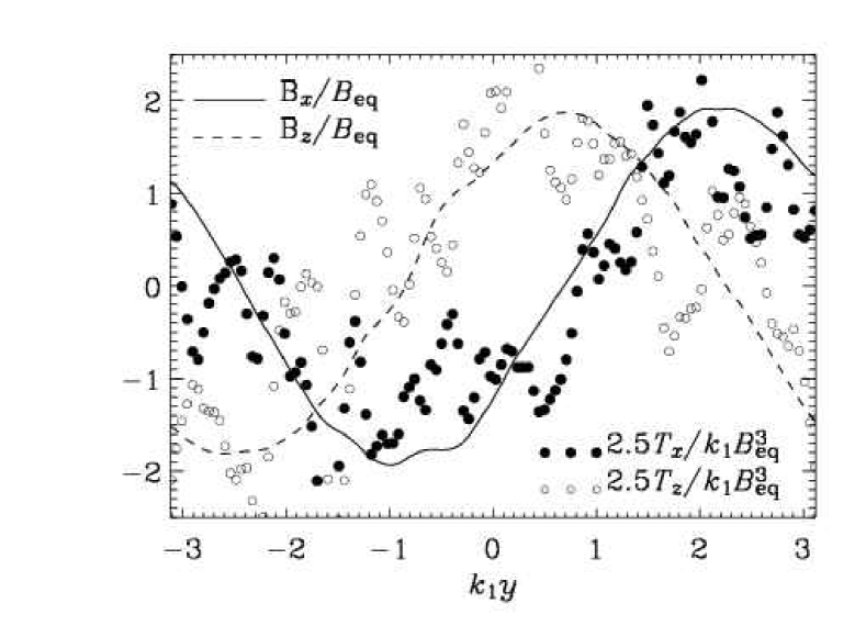
Figure 9.1: Comparison of the spatial dependence of two components of the mean magnetic field and the triple correlation in Run 3 of Ref. [4]. The magnetic field is normalized by the equipartition field strength, $B_{\rm eq}$, and the triple correlation is normalized by $k_{1}B_{\rm eq}^{3}$, but scaled by a factor of $2.5$ make it have a similar amplitude as the mean field. Note that $\overline{B}_{x}$ (solid line) correlates with $T_{x}$ (filled dots) and $\overline{B}_{z}$ (dashed line) correlates with $T_{z}$ (open dots). Adapted from Ref. [327].

In order to determine a meaningful value of $\tau$, it is important to get rid of the fluctuations of $\overline{\mbox{\boldmath${\mathcal{E}}$}}{}$, so time averaging is now necessary. The procedure is equivalent to that used in the passive scalar case [316], where a mean concentration gradient is imposed. Here, instead of imposing a gradient of the passive scalar concentration, one imposes a gradient in one component of the magnetic vector potential or, what is equivalent, a uniform magnetic field $\bm{B}_{0}$; see Ref. [327]. The deviations from the imposed field are treated as fully periodic in all three directions.

The simulations produce average values for the three quantities,

$$\alpha=\langle\overline{\mbox{\boldmath${\mathcal{E}}$}}{}\cdot\overline{\bm{B}}\rangle_{t}/\langle\overline{\bm{B}}^{2}\rangle_{t},\quad\tilde{\alpha}_{\rm K}=-{\textstyle{1\over 3}}\langle\overline{\bm{\omega}\cdot\bm{u}}\rangle_{t},\quad\tilde{\alpha}_{\rm M}={\textstyle{1\over 3}}\langle\overline{\bm{j}\cdot\bm{b}}\rangle_{t},$$ (9.8)

where $\langle...\rangle_{t}$ denotes combined time and volume averages. According to MTA, these three quantities are connected to each other via

$$\alpha=\tau\left(g_{\rm K}\tilde{\alpha}_{\rm K}+g_{\rm M}\tilde{\alpha}_{\rm M}\right),$$ (9.9)

where we have allowed for the presence of additional quenching factors, $g_{\rm K}(\overline{\bm{B}})$ and $g_{\rm M}(\overline{\bm{B}})$, in front of the $\tilde{\alpha}_{\rm K}$ and $\tilde{\alpha}_{\rm M}$ factors, respectively [394]. It turns out that for finite field strength the quenching factors, $g_{\rm K}$ and $g_{\rm M}$, are less than unity and, more importantly, they are slightly different from each other [394]. Using a combination of kinetically and magnetically forced turbulence simulations, it has been possible to calculate separately these two quenching functions multiplied by the normalized correction time, combined with the corresponding quenching functions, $\mbox{St}\,g_{\rm K}$ and $\mbox{St}\,g_{\rm M}$, respectively. Here we have defined

$$\mbox{St}=\tau u_{\rm rms}k_{\rm f}$$ (9.10)

as a nondimensional measure of the relaxation time [232, 301]. The result is shown in Fig. 9.2 as a function of the magnetic Reynolds number.

We recall that in the passive scalar case, St was found to converge to a value of about 3 in the limit of large Reynolds number and small values of $k_{\rm f}$ [316]. For the present case one finds that St is approximately unity for small field strengths, but may decrease like $B_{0}^{-3}$, once $B_{0}$ becomes comparable with the equipartition field strength, $B_{\rm eq}$; see Fig. 9.3.

Figure 9.2: Magnetic and kinetic Strouhal numbers as a function of $R_{\rm m}$ for different values of $B_{0}$ and $k_{\rm f}$. Here, kinetically and magnetically forced runs have been used to calculate separately $g_{\rm K}\neq g_{\rm M}$. Adapted from Ref. [327].

Figure 9.3: Magnetic and kinetic Strouhal numbers as a function of $B_{0}/B_{\rm eq}$ for $\eta=2\times 10^{-3}$ and $k_{\rm f}=1.5$. Kinetically and magnetically forced runs have been used to calculate separately $g_{\rm K}\neq g_{\rm M}$. Adapted from Ref. [327].

To summarize, the effect of the Lorentz forces is, to leading order, the addition of a current helicity contribution to $\tilde{\alpha}$ and hence to $\alpha$. There is an additional suppression effect which corresponds effectively to a dependence of $\tau$ on the strength of the mean field. This suppression seems however to be independent of or weakly dependent on the magnetic Reynolds number and is hence not the main limiting factor for the growth of large scale fields when the magnetic Reynolds number is large. (The last data point for $R_{\rm m}>100$ in the left hand panel of Fig. 9.2 seems to suggest a sudden decline, but it is not clear how reliable both this data point and the corresponding error estimate are.)

An immediate difficulty with having a small scale current helicity contribution to $\alpha$ in Eq. (9.5) is that one cannot directly incorporate this correction in a mean field model, because one only has information about the mean fields, $\overline{\mbox{\boldmath$J$}}$ and $\overline{\bm{B}}$, and not their fluctuations, $\bm{j}$ and $\bm{b}$. The solution to this problem is to invoke the magnetic helicity equation as an auxiliary equation to couple $\overline{\bm{j}\cdot\bm{b}}$ to the mean field equations. In other words, one has to solve both the mean field dynamo equation and the magnetic helicity equation simultaneously. We turn to this issue in the next section.

9.3 The dynamical quenching model

While conventional mean field theory is suitable to capture the structure of the mean field correctly, it has become clear that simple quenching expressions of the form (8.15) or (8.17) are unable to reproduce correctly the resistively limited saturation phase. Instead, they would predict saturation on a dynamical time scale, which is not only in contradiction with simulations [4], but it would also violate magnetic helicity conservation. The key to modeling the late saturation behavior correctly is to ensure that the magnetic helicity equation Eq. (8.5) is satisfied exactly at all times.

We begin with the usual mean field equation (6.7), which has to be solved for a given form of $\overline{\mbox{\boldmath${\mathcal{E}}$}}{}$. For $\alpha$ effect and possibly other mean field dynamos, the $\overline{\mbox{\boldmath${\mathcal{E}}$}}{}$ term produces magnetic helicity of the large scale field. The evolution equation of magnetic helicity of the mean field $\overline{\bm{B}}$ can be obtained in the usual fashion from the mean field induction equation. We restrict ourselves here to the case of a closed domain. In that case one obtains

$${\mathrm{d}\over\mathrm{d}t}\langle\overline{\mbox{\boldmath$A$}}\cdot\overline{\bm{B}}\rangle=2\langle\overline{\mbox{\boldmath${\mathcal{E}}$}}{}\cdot\overline{\bm{B}}\rangle-2\eta\langle\overline{\mbox{\boldmath$J$}}\cdot\overline{\bm{B}}\rangle,$$ (9.11)

which is independent of $\overline{\mbox{\boldmath$U$}}$. [Here, as earlier, angular brackets denote averaging over all space, while overbars denote suitably defined averages that could be two-dimensional (cf. Section 8.4) or one-dimensional if there is shear (cf. Section 8.9)]. One sees that there is a source term for the mean field helicity $\langle\overline{\mbox{\boldmath$A$}}\cdot\overline{\bm{B}}\rangle$, due to the presence of $\overline{\mbox{\boldmath${\mathcal{E}}$}}{}$. The $\langle\overline{\mbox{\boldmath$J$}}\cdot\overline{\bm{B}}\rangle$ term can be approximated by $k_{1}^{2}\langle\overline{\mbox{\boldmath$A$}}\cdot\overline{\bm{B}}\rangle$ and corresponds to a damping term. This merely reflects the fact that the operation of a mean field dynamo automatically leads to the growth of linkages between the toroidal and poloidal mean fields. Such linkages measure the helicity associated with the mean field. One then wonders how this mean field helicity arises? To understand this, we need to consider also the evolution of the small scale helicity $\langle\bm{a}\cdot\bm{b}\rangle$. Since the Reynolds rules apply, we have $\langle\bm{A}\cdot\bm{B}\rangle=\langle\overline{\mbox{\boldmath$A$}}\cdot\overline{\bm{B}}\rangle+\langle\bm{a}\cdot\bm{b}\rangle$, so the evolution equation for $\langle\bm{a}\cdot\bm{b}\rangle$ can be deduced by subtracting Eq. (9.11) from the evolution equation (8.5) for the total helicity. The fluctuating field then obeys the equation

$${\mathrm{d}\over\mathrm{d}t}\langle\bm{a}\cdot\bm{b}\rangle=-2\langle\overline{\mbox{\boldmath${\mathcal{E}}$}}{}\cdot\overline{\bm{B}}\rangle-2\eta\langle\bm{j}\cdot\bm{b}\rangle,$$ (9.12)

so the sum of Eqs. (9.11) and (9.12) gives Eq. (8.5) without any involvement of the $\overline{\mbox{\boldmath${\mathcal{E}}$}}{}$ term. We see therefore that the term $\langle\overline{\mbox{\boldmath${\mathcal{E}}$}}{}\cdot\overline{\bm{B}}\rangle$ merely transfers magnetic helicity between mean and fluctuating fields while conserving the total helicity!

In order to guarantee that the total helicity evolution equation (8.5) is always obeyed, Eq. (9.12) has to be solved as an auxiliary equation along with the mean field dynamo equation (6.7). From the previous two sections we have seen that $\overline{\mbox{\boldmath${\mathcal{E}}$}}{}$ is now determined by replacing the kinematic $\alpha$ effect by the residual $\alpha$ effect,

$$\alpha=-{\textstyle{1\over 3}}\tau\langle\bm{\omega}\cdot\bm{u}\rangle+{\textstyle{1\over 3}}\tau\langle\bm{j}\cdot\bm{b}\rangle\equiv\alpha_{\rm K}+\alpha_{\rm M},$$ (9.13)

and with no immediate modifications to $\eta_{\rm t}$. As mentioned before, subsequent modifications (i.e. quenching) of $\alpha_{\rm K}$ and $\eta_{\rm t}$ occur as a direct consequence of the decrease of turbulence intensity (which includes a decrease of the turbulent kinetic helicity) and/or the relaxation time (see Fig. 9.3) [148, 329, 373], but this is not a particularly dramatic effect, because it does not depend on $R_{\rm m}$. More important is the $\langle\bm{j}\cdot\bm{b}\rangle$ term in $\alpha_{\rm M}$; see Eq. (9.13). This term can be related to $\langle\bm{a}\cdot\bm{b}\rangle$ in Eq. (9.12) for a given spectrum of magnetic helicity. For a triply-periodic domain, using isotropy, we can write $\langle\bm{j}\cdot\bm{b}\rangle=k_{\rm f}^{2}\langle\bm{a}\cdot\bm{b}\rangle$, provided the averages involving $\bm{a}$, $\bm{b}$, and $\bm{j}$ are governed by components with wavenumber $k_{\rm f}$, where $k_{\rm f}$ is the approximate wavenumber of the energy-carrying scale. As mentioned earlier [6], the $k_{\rm f}$ factor may be attenuated by a $R_{\rm m}^{1/4}$ factor to account for the fact that for a $k^{-5/3}$ energy spectrum the $\langle\bm{j}\cdot\bm{b}\rangle$ term will pick up contributions from smaller scales. However, as described in Section 10, for such spectra, one has to retain a $k$-dependent $\tau(k)\propto k^{-2/3}$; this decreases for smaller scales making $\alpha_{M}$ (or $\alpha_{K}$) still dominated by contributions at the forcing scale, and so $\alpha_{M}$ (or $\alpha_{K}$) would be independent of $R_{\rm m}$ and Re. Also, new simulations [327] suggest that at scales smaller than the energy-carrying scale the field is no longer fully helical, and hence we do not expect there to be a $R_{\rm m}^{1/4}$ factor on the effective value of $k_{\rm f}$. The relaxation time $\tau$ can be expressed in terms of $B_{\rm eq}^{2}=u_{\rm rms}^{2}$ using $\eta_{\rm t}={\textstyle{1\over 3}}\tau u_{\rm rms}^{2}$. Furthermore, $\tau$, and therefore also $\eta_{\rm t}$, may still depend on $|\overline{\bm{B}}|$ in a way as shown in Fig. 9.3. (We recall that we have used $\rho_{0}=\mu_{0}=1$ throughout.)

Under the assumption $\alpha_{\rm K}={\rm const}{}$, the final set of equations can be summarized in the more compact form [6, 7]

$${\partial\overline{\bm{B}}\over\partial t}=\bm{\nabla}\times\left[\overline{\mbox{\boldmath$U$}}\times\overline{\bm{B}}+\alpha\overline{\bm{B}}-(\eta+\eta_{\rm t})\overline{\mbox{\boldmath$J$}}\right],$$ (9.14) $${\mathrm{d}\alpha\over\mathrm{d}t}=-2\eta_{\rm t}k_{\rm f}^{2}\left({\alpha\langle\overline{\bm{B}}^{2}\rangle-\eta_{\rm t}\langle\overline{\mbox{\boldmath$J$}}\cdot\overline{\bm{B}}\rangle\over B_{\rm eq}^{2}}+{\alpha-\alpha_{\rm K}\over\tilde{R}_{\rm m}}\right),$$ (9.15)

where $\tilde{R}_{\rm m}=\eta_{\rm t}/\eta$ is a modified definition of the microscopic magnetic Reynolds number; cf. Eq. (3.18). Simulations of forced turbulence with a decaying large scale magnetic field suggest $\eta_{\rm t}\approx(0.8...0.9)\times u_{\rm rms}/k_{\rm f}$ [395]. Thus, $\tilde{R}_{\rm m}=(0.8...0.9)\times R_{\rm m}$, but for all practical purposes the two are so close together that we assume from now on $\tilde{R}_{\rm m}=R_{\rm m}$. (As discussed in Section 3.4, $\eta$ cannot be replaced by a turbulent value, so $R_{\rm m}$ is in practice really very large!) We can now apply these equations to discuss various issues about the dynamical quenching of mean field dynamos.

9.3.1 Comparison with algebraic $\alpha$ quenching

In order to appreciate the nature of the solutions implied by Eqs. (9.14) and (9.15), consider first the long-time limit of a nonoscillatory dynamo. In this case the explicit time dependence in Eq. (9.15) may be neglected (adiabatic approximation [6]). Solving the resulting equation for $\alpha$ yields [9, 302]

$$\alpha={\alpha_{\rm K}+\eta_{\rm t}R_{\rm m}\langle\overline{\mbox{\boldmath$J$}}\cdot\overline{\bm{B}}\rangle/B_{\rm eq}^{2}\over 1+R_{\rm m}\langle\overline{\bm{B}}^{2}\rangle/B_{\rm eq}^{2}}\quad\mbox{(for $\mathrm{d}\alpha/\mathrm{d}t=0$)}.$$ (9.16)

Curiously enough, for the numerical experiments with an imposed large scale field over the scale of the box [311], where $\overline{\bm{B}}$ is spatially uniform and therefore $\overline{\mbox{\boldmath$J$}}=0$, one recovers the ‘catastrophic’ quenching formula (8.17),

$$\alpha={\alpha_{\rm K}\over 1+R_{\rm m}\langle\overline{\bm{B}}^{2}\rangle/B_{\rm eq}^{2}}\quad\mbox{(for $\overline{\mbox{\boldmath$J$}}=0$)},$$ (9.17)

which implies that $\alpha$ becomes quenched when $\langle\overline{\bm{B}}^{2}\rangle/B_{\rm eq}^{2}=R_{\rm m}^{-1}\approx 10^{-8}$ for the sun, and for even smaller fields for galaxies.

On the other hand, if the mean field is not imposed but maintained by dynamo action, $\overline{\bm{B}}$ cannot be spatially uniform and then $\overline{\mbox{\boldmath$J$}}$ is finite. In the case of a Beltrami field [4], $\langle\overline{\mbox{\boldmath$J$}}\cdot\overline{\bm{B}}\rangle/\langle\overline{\bm{B}}^{2}\rangle\equiv\tilde{k}_{\rm m}$ is some effective wavenumber of the large scale field with $\tilde{k}_{\rm m}\leq k_{\rm m}$. Since $R_{\rm m}$ enters both the numerator and the denominator, $\alpha$ tends to $\eta_{\rm t}\tilde{k}_{\rm m}$, i.e.

$$\alpha\to\eta_{\rm t}\tilde{k}_{\rm m}\quad\mbox{(for $\overline{\mbox{\boldmath$J$}}\neq 0$ and $\overline{\mbox{\boldmath$J$}}\parallel\overline{\bm{B}}$)}.$$ (9.18)

Compared with the kinematic estimate, $\alpha_{\rm K}\approx\eta_{\rm t}\tilde{k}_{\rm f}$, $\alpha$ is only quenched by the scale separation ratio $\tilde{k}_{\rm m}/\tilde{k}_{\rm f}$.

It remains possible, however, that $\eta_{\rm t}$ is suppressed via a quenching of $\tau$ (see Fig. 9.3). Thus, the question of how strongly $\alpha$ is quenched in the sun or the galaxy, has been diverted to the question of how strongly $\eta_{\rm t}$ is quenched [6]. Note that quasi-linear treatments or MTA do not predict $\eta_{t}$ quenching at the lowest order and for weak mean fields [396, 397]. One way to determine $\eta_{\rm t}$ and its possible quenching is by looking at numerical solutions of cyclic dynamos with shear ($\alpha\Omega$-type dynamos), because in the saturated state the cycle frequency is equal to $\eta_{\rm t}\tilde{k}_{\rm m}^{2}$. The best agreement between models and simulations is achieved when $\eta_{\rm t}$ begins to be quenched when $\langle\overline{\bm{B}}^{2}\rangle/B_{\rm eq}^{2}$ is around 0.3; see Ref. [6] for details. This means that $\eta_{\rm t}$ is only quenched non-catastrophically. This is consistent with the quenching of $\tau$; see Figs. 9.2 and 9.3. However, more detailed work at larger magnetic Reynolds numbers needs to be done – preferentially in more realistic geometries that could be more readily applied to stars and galaxies.

9.3.2 $\alpha^{2}$ dynamos

For $\alpha^{2}$ dynamos in a periodic box a special situation arises, because then the solutions are degenerate in the sense that $\overline{\mbox{\boldmath$J$}}$ and $\overline{\bm{B}}$ are parallel to each other. Therefore, the term $\langle\overline{\mbox{\boldmath$J$}}\cdot\overline{\bm{B}}\rangle\overline{\bm{B}}$ is the same as $\langle\overline{\bm{B}}^{2}\rangle\overline{\mbox{\boldmath$J$}}$, which means that in the mean EMF the term $\alpha\overline{\bm{B}}$, where $\alpha$ is given by Eq. (9.16), has a component that can be expressed as being parallel to $\overline{\mbox{\boldmath$J$}}$. In other words, the roles of turbulent diffusion (proportional to $\overline{\mbox{\boldmath$J$}}$) and $\alpha$ effect (proportional to $\overline{\bm{B}}$) cannot be disentangled. This is the force-free degeneracy of $\alpha^{2}$ dynamos in a periodic box [6]. This degeneracy is also the reason why for $\alpha^{2}$ dynamos the late saturation behavior can also be described by an algebraic (non-dynamical, but catastrophic) quenching formula proportional to $1/(1+R_{\rm m}\langle\overline{\bm{B}}^{2}\rangle)$ for both $\alpha$ and $\eta_{\rm t}$, as was done in Ref. [4]. To see this, substitute the steady state quenching expression for $\alpha$, from Eq. (9.16), into the expression for $\overline{\mbox{\boldmath${\mathcal{E}}$}}{}$. We find

$$\overline{\mbox{\boldmath${\mathcal{E}}$}}{}=\alpha\overline{\bm{B}}-(\eta+\eta_{\rm t})\overline{\mbox{\boldmath$J$}}={\alpha_{\rm K}+R_{\rm m}\eta_{\rm t}\langle\overline{\mbox{\boldmath$J$}}\cdot\overline{\bm{B}}\rangle/B_{\rm eq}^{2}\over 1+R_{\rm m}\langle\overline{\bm{B}}^{2}\rangle/B_{\rm eq}^{2}}\,\overline{\bm{B}}-\eta_{\rm t}\overline{\mbox{\boldmath$J$}}$$

$$={\alpha_{\rm K}\overline{\bm{B}}\over 1+R_{\rm m}\langle\overline{\bm{B}}^{2}\rangle/B_{\rm eq}^{2}}-{\eta_{\rm t}\overline{\mbox{\boldmath$J$}}\over 1+R_{\rm m}\langle\overline{\bm{B}}^{2}\rangle/B_{\rm eq}^{2}},$$ (9.19)

which shows that in the force-free case the adiabatic approximation, together with constant (unquenched) turbulent magnetic diffusivity, becomes equal to the pair of expressions where both $\alpha$ and $\eta_{\rm t}$ are catastrophically quenched. This force-free degeneracy is lifted in cases with shear or when the large scale field is no longer fully helical (e.g. in a nonperiodic domain, and in particular in the presence of open boundaries).

The dynamical quenching approach seems to be quite promising given that it describes correctly the $\alpha^{2}$ dynamo found in the simulations. There are however severe limitations that have to be overcome before it can be used in more realistic mean field models. Most importantly, the case of an inhomogeneous system, possibly one with boundaries, is not solved rigorously, although several promising approaches have been suggested [388, 394, 398, 399, 400, 401]. The difficulty is to generalize Eq. (9.12) to the non-homogeneous case of a mean magnetic helicity density, in a gauge-invariant manner. Only recently has this been attempted [154] by defining the magnetic helicity density of random fields as the density of correlated links. An alternate possibility is to consider directly the evolution equation of $\overline{\bm{j}\cdot\bm{b}}$ instead (as we do below). The other problem with boundaries is that one still requires a microscopic theory for the small scale losses of magnetic helicity through the boundaries [388, 394, 398]. In any case, a more sophisticated theory should still reproduce the homogeneous case, for which we now have now a fairly accurate quantitative understanding.

9.4 Saturation behavior of $\alpha^{2}$ and $\alpha\Omega$ dynamos

In the case of homogeneous $\alpha\Omega$ dynamos, a major fraction of the toroidal field can be generated by shear – independently of helicity. Therefore, $\langle\overline{\bm{B}}^{2}\rangle$ can be enhanced without producing much $\langle\overline{\mbox{\boldmath$J$}}\cdot\overline{\bm{B}}\rangle$. We discuss below the strength of the fields, both when the final resistive saturation limit has been reached and the case when $R_{\rm m}$ is so large that a quasi-static, non-resistive limit is more relevant (for example in galaxies).

9.4.1 Final field strength

In case one waits long enough, i.e. longer than the resistive time scale, we noted that the final field strength is determined by the condition $\langle\bm{J}\cdot\bm{B}\rangle=0$; or

$$\langle\overline{\mbox{\boldmath$J$}}\cdot\overline{\bm{B}}\rangle=-\langle\bm{j}\cdot\bm{b}\rangle.$$ (9.20)

In order to connect the current helicities with magnetic energies, we proceed as follows. First, one can quite generally relate the current and magnetic helicities by defining characteristic wavenumbers, $k_{\rm m}$ and $k_{\rm f}$, for the mean and fluctuating fields via

$$k_{\rm m}^{2}=\langle\overline{\mbox{\boldmath$J$}}\cdot\overline{\bm{B}}\rangle/\langle\overline{\mbox{\boldmath$A$}}\cdot\overline{\bm{B}}\rangle,$$ (9.21)

$$k_{\rm f}^{2}=\langle\bm{j}\cdot\bm{b}\rangle/\langle\bm{a}\cdot\bm{b}\rangle.$$ (9.22)

For a fully helical field, the same wavenumbers will also relate the current helicity and energy in the field. On the other hand, if the field is not fully helical, one can introduce efficiency factors $\epsilon_{\rm m}$ and $\epsilon_{\rm f}$ that characterize the helicity fractions of the mean and fluctuating fields, respectively, so we write

$$\langle\overline{\mbox{\boldmath$J$}}\cdot\overline{\bm{B}}\rangle/\langle\overline{\bm{B}}^{2}\rangle=k_{\rm m}\epsilon_{\rm m}\equiv\tilde{k}_{\rm m},$$ (9.23)

$$\langle\bm{j}\cdot\bm{b}\rangle/\langle\bm{b}^{2}\rangle=-k_{\rm f}\epsilon_{\rm f}\equiv-\tilde{k}_{\rm f}.$$ (9.24)

Here, $\tilde{k}_{\rm m}$ and $\tilde{k}_{\rm f}$ are are ‘effective wavenumbers’ for mean and fluctuating fields, respectively. In the final state, $k_{\rm m}$ will be close to the smallest wavenumber in the computational domain, $k_{1}$. In the absence of shear, $\epsilon_{\rm m}$ is of order unity, but it can be less if there is shear or if the boundary conditions do not permit fully helical large scale fields (see below). In the presence of shear, $\epsilon_{\rm m}$ turns out to be inversely proportional to the magnitude of the shear. The value of $\epsilon_{\rm f}$ and $\tilde{k}_{\rm f}$, on the other hand, is determined by small scale properties of the turbulence and is assumed known.

Both $k_{\rm m}$ and $k_{\rm f}$ are defined positive. However, $\epsilon_{\rm m}$ can be negative which is typically the case when $\alpha_{\rm K}<0$. The sign of $\epsilon_{\rm f}$ is defined such that it agrees with the sign of $\epsilon_{\rm m}$, i.e. both change sign simultaneously and hence $\tilde{k}_{\rm m}\tilde{k}_{\rm f}\geq 0$. In more general situations, $k_{\rm m}$ can be different from $k_{1}$. Using Eqs. (9.23) and (9.24) together with Eq. (8.7) we have

$$\tilde{k}_{\rm m}\langle\overline{\bm{B}}^{2}\rangle=\langle\overline{\mbox{\boldmath$J$}}\cdot\overline{\bm{B}}\rangle=-\langle\bm{j}\cdot\bm{b}\rangle=\tilde{k}_{\rm f}\langle\bm{b}^{2}\rangle,$$ (9.25)

and so in the final saturated state,

$$\langle\overline{\bm{B}}^{2}\rangle/\langle\bm{b}^{2}\rangle=\tilde{\kappa}_{\rm f}/\tilde{\kappa}_{\rm m},$$ (9.26)

which generalizes Eq. (8.8) to the case with fractional helicities; see also Eq. (79) of Ref. [159]. Of course, this analysis only applies to flows with helicity. In the nonhelical case, $\tilde{k}_{\rm m}=\tilde{k}_{\rm f}=0$, so Eq. (9.25) and Eq. (9.26) do not apply.

In the helical (or partially helical) case we can determine the final field strength of the mean and fluctuating fields. This is possible because in periodic geometry with homogeneous $\alpha$ effect the amplitude and energy of the dynamo wave is in general constant in time and does not vary with the cycle. We now use the mean field dynamo equation (9.14) to derive the evolution equation for the magnetic helicity of the large scale field, and apply it to the saturated state, so

$$0=\alpha\langle\overline{\bm{B}}^{2}\rangle-(\eta+\eta_{\rm t})\langle\overline{\mbox{\boldmath$J$}}\cdot\overline{\bm{B}}\rangle.$$ (9.27)

We also use the evolution equation (9.15) for the magnetic contribution to the $\alpha$ effect, applied again to the saturated state,

$$0={\alpha\langle\overline{\bm{B}}^{2}\rangle-\eta_{\rm t}\langle\overline{\mbox{\boldmath$J$}}\cdot\overline{\bm{B}}\rangle\over B_{\rm eq}^{2}}+{\alpha-\alpha_{\rm K}\over R_{\rm m}}.$$ (9.28)

Note both equations apply also when $\overline{\mbox{\boldmath$U$}}\neq 0$, because the $\overline{\mbox{\boldmath$U$}}\times\overline{\bm{B}}$ term has dropped out after taking the dot product with $\overline{\bm{B}}$. We now eliminate $\alpha$ from Eqs. (9.27) and (9.28) and thus derive expressions for the final steady state values of $\langle\overline{\bm{B}}^{2}\rangle\equiv B^{2}_{\rm fin}$ in terms of $B_{\rm eq}^{2}$ and $\langle\bm{b}^{2}\rangle\equiv b^{2}_{\rm fin}$, using Eq. (9.26). We get [6],

$${B^{2}_{\rm fin}\over B_{\rm eq}^{2}}={\alpha_{\rm K}-\eta_{\rm T}\tilde{k}_{\rm m}\over\eta_{\rm t}\tilde{k}_{\rm m}},\quad\quad{b^{2}_{\rm fin}\over B_{\rm eq}^{2}}={\alpha_{\rm K}-\eta_{\rm T}\tilde{k}_{\rm m}\over\eta_{\rm t}\tilde{k}_{\rm f}}.$$ (9.29)

In models where $\eta_{\rm t}$ is also quenched, both small scale and large scale field strengths increase as $\eta_{\rm t}$ is more strongly quenched. (Of course, regardless of how strongly $\eta_{\rm t}$ may be quenched, we always have from (9.26), $B^{2}_{\rm fin}/b^{2}_{\rm fin}=\tilde{\kappa}_{\rm f}/\tilde{\kappa}_{\rm m}$ in the final state.)

One can write $B_{\rm fin}$ in an instructive way, using the relevant dynamo control parameters for $\alpha^{2}$ and $\alpha\Omega$ dynamos, defined in Section 6.5.3. We generalize these for the present purpose and define

$$C_{\alpha}=\alpha_{\rm K}/(\eta_{\rm T}k_{\rm m}),\quad C_{\Omega}=S/(\eta_{\rm T}k^{2}_{\rm m}),$$ (9.30)

where $\alpha_{\rm K}$ is the initial value of $\alpha$ due to the kinetic helicity and $S=\Delta\Omega$ is a typical value of the shear in an $\alpha\Omega$ dynamo. From Eq. (9.27), the final steady state occurs when $\alpha=\eta_{\rm T}\tilde{k}_{\rm m}\equiv\alpha_{\rm crit}$ or a critical value of the dynamo parameter $C_{\alpha,\rm crit}=\alpha_{\rm crit}/\eta_{\rm T}k_{\rm m}$. One can then write, using (9.29),

$$B_{\rm fin}=\left({C_{\alpha}\over C_{\alpha,\rm crit}}-1\right)^{1/2}(1+R_{\rm m}^{-1})^{1/2}B_{\rm eq}.$$ (9.31)

For an $\alpha\Omega$ dynamo, the relevant dynamo number is given by $D_{0}=C_{\alpha}C_{\Omega}$ initially and in the final steady state, by $D_{\rm crit}=C_{\alpha,\rm crit}C_{\Omega}$, since the shear does not get affected by the nonlinear effects we consider. In this case the final mean field strength can be written as

$$B_{\rm fin}=\left({D_{0}\over D_{\rm crit}}-1\right)^{1/2}(1+R_{\rm m}^{-1})^{1/2}B_{\rm eq}.$$ (9.32)

Note once again that the above analysis only applies to flows with helicity. In the nonhelical case we have $\alpha_{\rm K}=\tilde{k}_{\rm m}=\tilde{k}_{\rm f}=0$, so Eq. (9.29) cannot be used. Nevertheless, without kinetic helicity one would still expect a finite value of $\langle\bm{b}^{2}\rangle$ because of small scale dynamo action. Furthermore, even in the fully helical case there can be substantial small scale contributions. Closer inspection of the runs of Ref. [4] reveals, however, that such contributions are particularly important only in the early kinematic phase of the dynamo.

In summary, the saturation field strength depends only on the scale separation ratio, see Eq. (9.26), and not, for example, on the intensity of the turbulence.

9.4.2 Early time evolution

During the early growth phase the magnetic helicity varies on time scales shorter than the resistive time, so the last term in the dynamical $\alpha$ quenching equation (9.15), which is proportional to $R_{\rm m}^{-1}\to 0$, can be neglected and so $\alpha$ evolves then approximately according to

$${\mathrm{d}\alpha\over\mathrm{d}t}\approx-2\eta_{\rm t}k_{\rm f}^{2}(\alpha-\eta_{\rm t}\tilde{k}_{\rm m}){\langle\overline{\bm{B}}^{2}\rangle\over B_{\rm eq}^{2}}.$$ (9.33)

This equation can be used to describe the end of the kinematic time evolution when $\langle\overline{\bm{B}}^{2}\rangle$ grows exponentially. (We refer to this phase as late ’kinematic’ because the slow resistive saturation has not yet set in, although of course $\alpha$ is already becoming suppressed due to growth of the current helicity.) We see from (9.33) that the $-2\eta_{\rm t}k_{\rm f}^{2}\alpha$ term leads to a reduction of $\alpha$. This leads to a dynamical reduction of $\alpha$ until it becomes comparable to $\eta_{\rm t}\tilde{k}_{\rm m}$, shutting off any further reduction. Therefore, the early time evolution leads to a nearly $R_{\rm m}$-independent growth phase. At the end of this growth phase a fairly significant large scale field should be possible [5, 6, 7]. The basic physical reason is that the suppression of $\alpha$ occurs due to the growth of small scale current helicity which, in turn, is the result of a growth of the small scale magnetic helicity. Since magnetic helicity is nearly conserved for $R_{\rm m}\gg 1$, this implies a corresponding growth of oppositely signed large scale magnetic helicity and hence the large scale field. We mention, however, that numerical simulations [402] have not been able to confirm a sharp transition from exponential to linear (resistively limited) growth, as seen in Fig. 9.4, which shows a numerical solution of Eqs. (9.14) and (9.15); see Refs [6, 403]. The absence of a sharp cross-over from exponential to linear growth in the turbulence simulations could be related to the fact that several large scale modes are competing, causing an extra delay in the selection of the final mode.

Figure 9.4: Evolution of $\langle\overline{\bm{B}}^{2}\rangle$ and $\langle\bm{b}^{2}\rangle$ (solid and dashed lines, respectively) in a doubly-logarithmic plot for an $\alpha^{2}$ dynamo with $\eta_{\rm t}=\mbox{const}$ for a case with $k_{\rm f}/k_{1}=10$. Note the abrupt initial saturation after the end of the kinematic exponential growth phase with $\langle\overline{\bm{B}}^{2}\rangle/\langle\bm{b}^{2}\rangle\sim 0.1$, followed by a slow saturation phase during which the field increases to its final super-equipartition value with $\langle\overline{\bm{B}}^{2}\rangle/\langle\bm{b}^{2}\rangle\sim 10$ [403].

In the following discussion we restrict ourselves to the case where $\eta$ is small or $R_{\rm m}\gg 1$. Magnetic helicity is then well conserved and this conservation requires that

$$\langle\overline{\mbox{\boldmath$A$}}\cdot\overline{\bm{B}}\rangle\approx-\langle\bm{a}\cdot\bm{b}\rangle\quad\mbox{(for $t\leq t_{\rm kin}$)}.$$ (9.34)

Here the time $t=t_{\rm kin}$ marks the end of the exponential growth phase (and thus the ‘initial’ saturation time $t_{\rm sat}$ used in Ref. [4]). This time is determined by the condition that the term in parenthesis in Eq. (9.33) becomes significantly reduced, i.e. $\alpha$ becomes comparable to $\eta_{\rm t}\tilde{k}_{\rm m}$. We would like to estimate the field strengths of the large and small scale fields by this time. The helicity conservation constraint (9.34), and the definitions in (9.21), (9.22) and (9.23), give

$$\alpha_{\rm M}={\textstyle{1\over 3}}\tau\langle\bm{j}\cdot\bm{b}\rangle={\textstyle{1\over 3}}\tau k_{\rm f}^{2}\langle\bm{a}\cdot\bm{b}\rangle=-{\textstyle{1\over 3}}\tau k_{\rm f}^{2}\langle\overline{\mbox{\boldmath$A$}}\cdot\overline{\bm{B}}\rangle=-\eta_{\rm t}{k_{\rm f}^{2}\over k_{\rm m}^{2}}{\tilde{k}_{\rm m}\langle\bm{B}^{2}\rangle\over B_{\rm eq}^{2}}.$$ (9.35)

We use this in Eq. (9.13) for $\alpha$ and demand that $\alpha$, as governed by the dynamical quenching equation (9.15), settles down to a quasi steady state by $t=t_{\rm kin}$. We then get for the mean squared strength of the large scale field at $t=t_{\rm kin}$,

$${B_{\rm kin}^{2}\over B_{\rm eq}^{2}}={\alpha_{\rm K}-\eta_{\rm t}\tilde{k}_{\rm m}\over\eta_{\rm t}\tilde{k}_{\rm m}}{k_{\rm m}^{2}\over k_{\rm f}^{2}}-R_{M}^{-1}\approx{\alpha_{\rm K}-\eta_{\rm t}\tilde{k}_{\rm m}\over\tilde{\iota}\eta_{\rm t}\tilde{k}_{\rm m}}{k_{\rm m}^{2}\over k_{\rm f}^{2}},$$ (9.36)

where the effect of a finite $R_{\rm m}$ has been included through an approximate correction factor [6]

$$\tilde{\iota}=1+R_{\rm m}^{-1}{k_{\rm f}/\epsilon_{\rm f}\over k_{\rm m}/\epsilon_{\rm m}}.$$ (9.37)

The strength of the small scale field at $t=t_{\rm kin}$ is given by using (9.34),

$$b_{\rm kin}^{2}={k_{\rm f}/\epsilon_{\rm f}\over k_{\rm m}/\epsilon_{\rm m}}B_{\rm kin}^{2}={\alpha_{\rm K}-\eta_{\rm t}\tilde{k}_{\rm m}\over\tilde{\iota}\eta_{\rm t}\tilde{k}_{\rm f}}B_{\rm eq}^{2}.$$ (9.38)

Not surprisingly, at the end of the kinematic phase the small scale magnetic energy is almost the same as in the final state; see Eq. (9.29). However, the large scale magnetic energy is still by a factor $k_{\rm m}^{2}/k_{\rm f}^{2}$ smaller than in the final state ($\epsilon_{\rm m}$ may be somewhat different in the two stages). This result was also obtained by Subramanian [7] using a similar approach.

These expressions can be further clarified by noting that the fractional helicity of the small scale field is likely to be similar to that of the forcing velocity field. We can then write $\langle\bm{\omega}\cdot\bm{u}\rangle\approx\epsilon_{\rm f}k_{\rm f}\langle\bm{u}^{2}\rangle$; so $\alpha_{\rm K}\approx\eta_{\rm t}\epsilon_{\rm f}k_{\rm f}$, and one arrives at [6]

$${B_{\rm kin}^{2}\over B_{\rm eq}^{2}}={k_{\rm m}/\epsilon_{\rm m}\over\tilde{\iota}k_{\rm f}/\epsilon_{\rm f}}\left(1-{\tilde{\kappa}_{\rm m}\over\tilde{\kappa}_{\rm f}}\right),$$ (9.39)

which shows that $B_{\rm kin}$ can be comparable to and even in excess of $B_{\rm eq}$, especially when $\epsilon_{\rm m}$ is small (i.e. for strong shear). This is of interest in connection with the question of why the magnetic field in so many young galaxies can already have equipartition field strengths.

As emphasized in Ref. [5], even for an $\alpha^{2}$ dynamo, the initial evolution to $B_{\rm kin}$ is significantly more optimistic an estimate than what could have been expected based on lorentzian $\alpha$ quenching. In the case of an $\alpha\Omega$ dynamo [6, 7], one could have $\tilde{k}_{\rm m}\ll k_{\rm m}$, and so $B_{\rm kin}$ can be correspondingly larger. In fact, for

$$\epsilon_{\rm m}/\epsilon_{\rm f}\leq k_{\rm m}/k_{\rm f},$$ (9.40)

the large scale field begins to be of order $B_{\rm eq}$ and exceeds the small scale field already during the kinematic growth phase.

It is once again instructive to express $B_{\rm kin}$ in terms of the dynamo control parameters, $C_{\alpha}$ and $C_{\Omega}$. Note that for small $\eta$, or $R_{\rm m}\gg 1$, $\alpha_{\rm crit}=\eta_{\rm T}\tilde{k}_{\rm m}\approx\eta_{\rm t}\tilde{k}_{\rm m}$ and $\tilde{\iota}\approx 1$. One can then write

$$B_{\rm kin}={k_{\rm m}\over k_{\rm f}}\left[{C_{\alpha}\over C_{\alpha,\rm crit}}-1\right]^{1/2}B_{\rm eq}.$$ (9.41)

For an $\alpha\Omega$ dynamo with dynamo number $D_{0}=C_{\alpha}C_{\Omega}$ and a critical value $D_{\rm crit}=C_{\alpha,\rm crit}C_{\Omega}$, we have (assuming shear does not get affected) [7]

$$B_{\rm kin}={k_{\rm m}\over k_{\rm f}}\left[{D_{0}\over D_{\rm crit}}-1\right]^{1/2}B_{\rm eq}.$$ (9.42)

We can estimate how strong the shear has to be for the large scale field to be comparable to $B_{\rm eq}$. Since $\alpha_{\rm K}\approx\eta_{\rm t}\epsilon_{\rm f}k_{\rm f}$, $C_{\alpha}\approx\epsilon_{\rm f}(k_{\rm f}/k_{\rm m})$, or $k_{\rm m}/k_{\rm f}\approx\epsilon_{\rm f}/C_{\alpha}$. Using $D_{0}=C_{\alpha}C_{\Omega}$, we can rewrite (9.42) as

$$B_{\rm kin}=\left[{C_{\Omega}\epsilon_{\rm f}^{2}\over C_{\alpha}D_{\rm crit}}-{k_{\rm m}^{2}\over k_{\rm f}^{2}}\right]^{1/2}B_{\rm eq}.$$ (9.43)

Now $k_{\rm m}/k_{\rm f}\ll 1$ in general. So $B_{\rm kin}$ can become comparable to $B_{\rm eq}$ provided the shear is strong enough that $C_{\Omega}\epsilon_{\rm f}^{2}>C_{\alpha}D_{\rm crit}$. For dynamo action to be possible, one also requires $C_{\Omega}C_{\alpha}>D_{\rm crit}$ or $C_{\alpha}>D_{\rm crit}/C_{\Omega}$. Combining these two inequalities, we see that large scale fields can become comparable to the equipartition fields if $C_{\Omega}\mathrel{\mathchoice{\vbox{\offinterlineskip\halign{\hfil$\displaystyle#$\hfil\cr>\cr\sim\cr}}}{\vbox{\offinterlineskip\halign{\hfil$\textstyle#$\hfil\cr>\cr\sim\cr}}}{\vbox{\offinterlineskip\halign{\hfil$\scriptstyle#$\hfil\cr>\cr\sim\cr}}}{\vbox{\offinterlineskip\halign{\hfil$\scriptscriptstyle#$\hfil\cr>\cr\sim\cr}}}}D_{\rm crit}/\epsilon_{\rm f}$. The critical dynamo number $D_{\rm crit}$ will depend on the physical situation at hand; $D_{\rm crit}=2$ for a one dimensional $\alpha\Omega$ dynamo with periodic boundary conditions and homogeneous $\alpha_{\rm K}$. Further, in simulations of rotating convection, $\epsilon_{\rm f}\approx 0.03$ [203]; assuming that this relatively low value of $\epsilon_{\rm f}$ is valid in more realistic simulations, we have $C_{\Omega}\mathrel{\mathchoice{\vbox{\offinterlineskip\halign{\hfil$\displaystyle#$\hfil\cr>\cr\sim\cr}}}{\vbox{\offinterlineskip\halign{\hfil$\textstyle#$\hfil\cr>\cr\sim\cr}}}{\vbox{\offinterlineskip\halign{\hfil$\scriptstyle#$\hfil\cr>\cr\sim\cr}}}{\vbox{\offinterlineskip\halign{\hfil$\scriptscriptstyle#$\hfil\cr>\cr\sim\cr}}}}2/\epsilon_{\rm f}\approx 60$ as the condition for which the large scale field becomes comparable to $B_{\rm eq}$. (Note that when the large scale field becomes comparable to $B_{\rm eq}$, quenching due to the large scale field itself will become important, a process we have so far ignored.) This condition on the shear, could be satisfied for stellar dynamos but it is not likely to be satisfied for galactic dynamos, where typically $D_{0}/D_{\rm crit}\sim 2$ (cf. Section 11.5).

During the subsequent resistively limited saturation phase the energy of the large scale field grows first linearly, i.e.

$$\langle\overline{\bm{B}}^{2}\rangle\approx B_{\rm kin}^{2}+2\eta k_{\rm m}^{2}(t-t_{\rm kin})\quad\mbox{(for $t>t_{\rm kin}$)},$$ (9.44)

and saturates later in a resistively limited fashion; see Eq. (8.13).

9.4.3 Comparison with simulations

In order to compare the dynamical quenching model with simulations of turbulent oscillatory dynamos with shear [386], it is important to consider the same geometry and shear profile, i.e. sinusoidal shear, $\overline{\mbox{\boldmath$U$}}=(0,Sk_{1}^{-1}\cos k_{1}x,0)$, and a mean field $\overline{\bm{B}}=\overline{\bm{B}}(x,z,t)$. We discuss here the results of Ref. [6], where simulations of Ref. [386] are compared with dynamical quenching models using either a fixed value of $\eta_{\rm t}$ or, following earlier suggestions [4, 5], a turbulent diffusivity that is quenched in the same way as $\alpha$, i.e. $\eta_{\rm t}\propto\alpha$.

Both simulation and model show dynamo waves traveling in the positive $z$-direction at $x=\pm\pi$ and in the negative $z$-direction at $x=0$, which is consistent with the three-dimensional simulations using negative values of $\alpha_{\rm K}$, which affects the direction of propagation of the dynamo waves.

It turns out that in all models the values of $b^{2}_{\rm fin}$ are smaller than in the simulations. This is readily explained by the fact that the model does not take into account small scale dynamo action resulting from the nonhelical component of the flow. Comparing simulations with different values of $R_{\rm m}$, the cycle frequency changes by a factor compatible with the ratio of the two magnetic Reynolds numbers. This is not well reproduced by a quenching expression for $\eta_{\rm t}$ that is independent of $R_{\rm m}$. On the other hand, if $\eta_{\rm t}$ is assumed to be proportional to $\alpha$, then $\omega_{\rm cyc}$ becomes far smaller than what is seen in the simulations. A possible remedy would be to have some intermediate quenching expression for $\eta_{\rm t}$. We should bear in mind, however, that the present model ignores the feedback from the large scale fields. Such feedback is indeed present in the simulations, which also show much more chaotic behavior than the model [6].

In conclusion the dynamical quenching model predicts saturation amplitudes of the large scale field that are smaller than the equipartition field strength by a factor that is equal to the ratio of the turbulent eddy size to the system size, and hence independent of the magnetic Reynolds number. The field strengths can be much larger if the dynamo involves shear and is highly supercritical. This may be relevant to explaining the amplitudes of fields in stars, but in galaxies the effect of shear is not likely to be strong enough to explain large scale galactic fields without additional effects such as a small scale helicity flux (see below and Section 11.5). One the other hand, for the sun and sun-like stars, the main issue is the cycle period. No conclusive answer can be given until there is definitive knowledge about the quenching of the turbulent magnetic diffusivity, $\eta_{\rm t}$ and the effect of current helicity fluxes out of the domain. The more $\eta_{\rm t}$ is quenched, the longer the cycle period can become, unless there are significant losses of magnetic helicity through the open boundaries that all these bodies must have. Before discussing this in Section 9.6 we first make a few historical remarks and also address the question of how close to being resistively limited the solar cycle might be. The answer is somewhat surprising: not much!

9.4.4 Historical remarks

The explicit time dependence of the $\alpha$ quenching equation (9.15) was first proposed by Kleeorin and Ruzmaikin [9] in an early paper of 1982; see also the book by Zeldovich et al. [222] and a later paper by Kleeorin et al. [404]. For a long time the true significance of the long time scale introduced by Eq. (9.15) remained unclear. It was therefore not surprising that early work focused exclusively on explaining the chaotic nature of the solar cycle [10, 11, 12].

The steady state limit (9.16) of Eq. (9.15) was first analyzed by Gruzinov & Diamond [302] and Bhattacharjee & Yuan [303] and so the connection with catastrophic quenching was established. When the issue of a resistively limited saturation of $\alpha^{2}$ dynamos in periodic boxes was raised [4], the possible connection with Eq. (9.15) was blurred by the fact that the simulation data could well be described by simultaneous and catastrophic quenching of $\alpha$ and $\eta_{\rm t}$. In the paper by Field and Blackman [5] it was first proposed and quantitatively demonstrated that resistively slow saturation can be explained in terms of mean field theory with a current helicity correction to the $\alpha$ effect, as calculated by Pouquet, Frisch and Léorat [304] already in 1976. This result was then recast to take the form of Eq. (9.15), which has to be solved simultaneously with the dynamo equation Eq. (9.14), and the connection with simultaneous catastrophic quenching of $\alpha$ and $\eta_{\rm t}$ was understood as a special case that applies only to $\alpha^{2}$ dynamos [6]. Equations (9.14) and (9.15) were also used to estimate the minimal mean magnetic fields which could be obtained in galaxies, in spite of the helicity constraint [7], ignoring however the effects of magnetic and current helicity fluxes. Blackman & Field [48, 405] proposed that such helicity fluxes could alleviate catastrophic $\alpha$ quenching. Kleeorin and coworkers [394, 398, 399] found that helicity fluxes are indeed likely to lead to substantially increased saturation field strengths, while Vishniac & Cho [388] suggested that helicity fluxes could even drive a dynamo effect of its own.

The generalization of Eq. (9.15) to spatially non-uniform systems is nontrivial, since one has to define a gauge invariant magnetic helicity even for systems with boundaries. This concept is helpful in simple cases of homogeneous turbulence, but it needs to be generalized to the more interesting inhomogeneous case, which has only been attempted recently [154]. This is why we have shifted the attention to considering the evolution of current helicity instead [391]; see Section 10.4. The current helicity is gauge invariant, directly observable and appears explicitly in the back reaction term in $\alpha$.

Initial attempts to verify the importance of helicity fluxes in open box simulations failed [392], and it was only in the presence of shear that evidence for accelerated field saturation emerged [55]. The agreement between simulations and mean field theory with helicity fluxes is still not fully satisfactory. In particular, with moderately strong helicity fluxes the solutions of the mean field model predict saturation energies that decrease inversely proportional with magnetic Reynolds number, unless the magnitude of the helicity flux exceeds a certain threshold [406].

It should also be pointed out that the explanation of catastrophic quenching in terms of magnetic helicity conservation is not generally accepted; see Refs [377, 407] for recent reviews. An alternative explanation for the catastrophic quenching phenomenon is in terms of a suppression of chaos [408]. Unfortunately, at the moment there is no quantitative theory that explains the magnetic Reynolds number dependence of this suppression.

9.5 How close to being resistively limited is the 11 year cycle?

In this section we present an estimate of the amount of magnetic helicity, $H$, that is expected to be produced and destroyed during the 11 year cycle [159]. We also need to know what fraction of the magnetic field takes part in the 11-year cycle. Here we are only interested in the relative magnetic helicity in one hemisphere. Following an approach similar to that of Berger [151], one can bound the rate of change of magnetic helicity, as given by Eq. (8.5), in terms of the rate of Joule dissipation, $Q_{\rm Joule}$, and magnetic energy, $M$, i.e.

$$\left|{\mathrm{d}H\over\mathrm{d}t}\right|\leq 2\eta\langle\bm{J}\cdot\bm{B}\rangle V\leq 2\eta\sqrt{\langle\bm{J}^{2}\rangle\langle\bm{B}^{2}\rangle}V\equiv 2\sqrt{2\eta Q_{\rm Joule}M},$$ (9.45)

where $V$ is the volume, $\langle\eta\bm{J}^{2}\rangle V=Q_{\rm Joule}$ the Joule heat, and $\langle{\textstyle{1\over 2}}\bm{B}^{2}\rangle V=M$ the magnetic energy. For an oscillatory dynamo, all three variables, $H$, $M$, and $Q_{\rm Joule}$ vary in an oscillatory fashion with a cycle frequency $\omega_{\rm cyc}$ of magnetic energy (corresponding to 11 years for the sun – not 22 years), so we estimate $|\mathrm{d}H/\mathrm{d}t|\mathrel{\mathchoice{\vbox{\offinterlineskip\halign{\hfil$\displaystyle#$\hfil\cr<\cr\sim\cr}}}{\vbox{\offinterlineskip\halign{\hfil$\textstyle#$\hfil\cr<\cr\sim\cr}}}{\vbox{\offinterlineskip\halign{\hfil$\scriptstyle#$\hfil\cr<\cr\sim\cr}}}{\vbox{\offinterlineskip\halign{\hfil$\scriptscriptstyle#$\hfil\cr<\cr\sim\cr}}}}\omega_{\rm cyc}|H|$ and $|\mathrm{d}M/\mathrm{d}t|\mathrel{\mathchoice{\vbox{\offinterlineskip\halign{\hfil$\displaystyle#$\hfil\cr<\cr\sim\cr}}}{\vbox{\offinterlineskip\halign{\hfil$\textstyle#$\hfil\cr<\cr\sim\cr}}}{\vbox{\offinterlineskip\halign{\hfil$\scriptstyle#$\hfil\cr<\cr\sim\cr}}}{\vbox{\offinterlineskip\halign{\hfil$\scriptscriptstyle#$\hfil\cr<\cr\sim\cr}}}}Q_{\rm Joule}\mathrel{\mathchoice{\vbox{\offinterlineskip\halign{\hfil$\displaystyle#$\hfil\cr<\cr\sim\cr}}}{\vbox{\offinterlineskip\halign{\hfil$\textstyle#$\hfil\cr<\cr\sim\cr}}}{\vbox{\offinterlineskip\halign{\hfil$\scriptstyle#$\hfil\cr<\cr\sim\cr}}}{\vbox{\offinterlineskip\halign{\hfil$\scriptscriptstyle#$\hfil\cr<\cr\sim\cr}}}}\omega_{\rm cyc}M$, and obtain

$$\omega_{\rm cyc}|H|\leq 2\sqrt{2\eta\omega_{\rm cyc}}\,M.$$ (9.46)

This leads to the inequality [159, 300]

$$|H|/(2M)\leq\ell_{\rm skin},$$ (9.47)

where $\ell_{\rm skin}=\sqrt{2\eta/\omega_{\rm cyc}}$ is the skin depth, here associated with the 11 year frequency $\omega_{\rm cyc}$. Thus, the maximum magnetic helicity that can be generated and dissipated during one cycle is characterized by the length scale $|H|/(2M)$, which has to be less than the skin depth $\ell_{\rm skin}$.

For $\eta$ we have to use the Spitzer resistivity [see Eq. (3.14)], so $\eta$ increases from about $10^{4}\,{\rm cm}^{2}/{\rm s}$ at the base of the convection zone to about $10^{7}\,{\rm cm}^{2}/\,{\rm s}$ near the surface layers and decreases again in the solar atmosphere, see Eq. (3.14). Using $\omega_{\rm cyc}=2\pi/(11\,{\rm yr})=2\times 10^{-8}\,{\rm s}^{-1}$ for the relevant frequency at which $H$ and $M$ vary, we have $\ell_{\rm skin}\approx 10\,{\rm km}$ at the bottom of the convection zone and $\ell_{\rm skin}\approx 300\,{\rm km}$ at the top.

The value of $\ell_{\rm skin}$ should be compared with the value $|H|/(2M)$ that can be obtained from dynamo models [159]. For a sphere (or rather a half-sphere) with open boundary conditions and volume $V$ (for example the northern hemisphere), one has to use the gauge-invariant relative magnetic helicity of Berger and Field [150]; see Eq. (3.35) and Section 3.4. We assume that the dynamo saturates such that most of the magnetic helicity is already in the large scales [cf. Eq. (8.11)], so $H$ can be estimated from a mean field model. We also assume that magnetic helicity is not continuously being pumped back and forth between large and small scales. While this remains a hypothetic possibility, it should be noted that this has never been seen in simulations. With these reservations in mind, we now employ an axisymmetric mean field, which can be written as $\overline{\bm{B}}=b\hat{\bm{\phi}}+\bm{\nabla}\times(a\hat{\bm{\phi}})$, it turns out that the relative magnetic helicity integral is simply [159]

$$H=2\int_{V}ab\,\mathrm{d}V\quad\mbox{(axisymmetry)}.$$ (9.48)

The results of model calculations show that [159], when the ratio of poloidal field at the pole to the maximum toroidal field inside the convection zone, $B_{\rm pole}/B_{\rm belt}$, is in the range consistent with observations, $B_{\rm pole}/B_{\rm belt}=(1...3)\times 10^{-4}$, then the ratio $H_{\rm N}/(2M_{\rm N}R)$ is around $(2-5)\times 10^{-4}$ for models with latitudinal shear. (Here, the subscript ‘N’ refers to the northern hemisphere.) This confirms the scaling with the poloidal to toroidal field ratio [386],

$$H_{\rm N}/(2M_{\rm N}R)={\cal O}(B_{\rm pol}/B_{\rm tor})\mathrel{\mathchoice{\vbox{\offinterlineskip\halign{\hfil$\displaystyle#$\hfil\cr>\cr\sim\cr}}}{\vbox{\offinterlineskip\halign{\hfil$\textstyle#$\hfil\cr>\cr\sim\cr}}}{\vbox{\offinterlineskip\halign{\hfil$\scriptstyle#$\hfil\cr>\cr\sim\cr}}}{\vbox{\offinterlineskip\halign{\hfil$\scriptscriptstyle#$\hfil\cr>\cr\sim\cr}}}}B_{\rm pole}/B_{\rm belt}.$$ (9.49)

Given that $R=700\,{\rm Mm}$ this means that $H_{\rm N}/(2M_{\rm N})\approx 70...200\,{\rm km}$, which would be comparable to the value of $\ell_{\rm skin}$ near the upper parts of the solar convection zone.

The surprising conclusion is that the amount of mean field helicity that needs to be generated in order to explain the large scale solar magnetic fields is actually so small, that it may be plausible that microscopic magnetic diffusion could still play a role in the solar dynamo. In other words, although open boundary effects may well be important for understanding the time scale of the dynamo, the effect does not need to be extremely strong. Of course, no quantitatively accurate predictions can be made, because the result depends on the model.

9.6 Open boundaries

In the preceding sections we made the assumption that no magnetic helicity flows through the boundaries. This is of course unrealistic, and on the sun magnetic helicity losses are indeed observed; see Section 2.1.2. In the presence of open boundaries one has to use the relative magnetic helicity, as defined in Eq. (3.38). In this equation there emerges a surface term, $2\oint(\bm{E}\times\bm{A}^{\rm ref})\cdot\mathrm{d}\bm{S}$, which is due to helicity fluxes. The importance of helicity fluxes was already demonstrated in Section 8.11. The question is how important is this effect and can it possibly alleviate the magnetic helicity constraint by allowing the $\alpha$ effect to be less strongly quenched [405].

9.6.1 Historical remarks

The question of how magnetic helicity losses could alleviate the problem of catastrophic quenching and resistively limited saturation and perhaps cycle periods remained at first unclear when this idea was originally proposed [398, 405]. Simulations of helically forced turbulence in an open domain, using a vertical field boundary condition ($\bm{B}\times\hat{\mbox{\boldmath$n$}}{}=0$), showed a shorter saturation time. However, this was at the expense of a reduced saturation amplitude [392]. This somewhat frustrating result raised concerns whether magnetic helicity losses could even help in principle. This was then the reason for performing the co-called vacuum cleaner experiment where small scale magnetic fields were artificially removed in regular intervals via Fourier filtering [159]. The main insight came when it was realized that it is not so much the boundary conditions as such that have a positive effect in alleviating the magnetic helicity constraint, but the fact that there is a magnetic helicity flux also inside the domain, such that magnetic helicity can actually be transported toward the boundaries. A leading candidate for this flux is the flux derived by Vishniac and Cho [388]. This flux will be derived and discussed further in Section 10.4.2.

There is another complication that led to considerable confusion. Magnetic helicity is defined as a volume integral (Section 3.4), and, because of the gauge problem, the concept of a magnetic helicity density does not exist. This has actually changed and a magnetic helicity density can actually be defined (for small scale fields) in terms of a density of linkages if there exists a meaningful separation into large scale and small scale fields [154]. Another important aspect was the realization that the quantity that we are primarily interested in, and that directly enters the magnetic $\alpha$ effect, is $\overline{\bm{j}\cdot\bm{b}}$. In working directly with $\overline{\bm{j}\cdot\bm{b}}$ there is of course no longer the comfort of dealing with a conserved quantity. Thus, the proper evolution equation for $\overline{\bm{j}\cdot\bm{b}}$ can no longer be inferred from total magnetic helicity conservation together with the evolution equation for the large scale field. Instead, $\overline{\bm{j}\cdot\bm{b}}$ has to be calculated directly using standard closure procedures [391]. There are now strong indications that an important prerequisite for obtaining a strong helicity flux is shear. However, shear has only recently been included in simulations with open boundaries; see Section 8.11 and Ref. [55]. Therefore, not too much analysis has been done on this type of problem yet.

In the following we present first a phenomenological model that explains the relative significance of large scale and small scale magnetic helicity losses. We then turn to speculative consequences for the observed solar field and demonstrate that small scale losses can alleviate the quenching problem – at least in principle.

9.6.2 A phenomenological model of magnetic helicity losses

It is instructive to discuss first a phenomenological description of magnetic helicity losses. We imagine that the loss of magnetic helicity across the boundary is accomplished by the turbulent exchange of eddies across the boundary. The rate of magnetic helicity loss is then proportional to some turbulent diffusivity coefficient, $\eta_{\rm m}$ or $\eta_{\rm f}$, for the losses from mean and fluctuating parts, respectively. Again, we assume that the small and large scale fields are maximally helical (or have known helicity fractions $\epsilon_{\rm m}$ and $\epsilon_{\rm f}$) and have opposite signs of magnetic helicity at small and large scales. The details can be found in Refs [49, 159]. The strength of this approach is that it is quite independent of mean field theory.

We proceed analogously to Section 8.5.2 where we used the magnetic helicity equation (8.5) for a closed domain to estimate the time derivative of the magnetic helicity of the mean field, $H_{1}$ (or $H_{\rm m}$, which is here the same), by neglecting the time derivative of the fluctuating field, $H_{\rm f}$. This is a good approximation after the fluctuating field has reached saturation, i.e. $t>t_{\rm sat}$. Thus, we have

$${{\rm d}H_{\rm m}\over{\rm d}t}+\underbrace{{{\rm d}H_{\rm f}\over{\rm d}t}}_{\mbox{neglected}}=-2\eta_{\rm m}k_{\rm m}^{2}H_{\rm m}-2\eta_{\rm f}k_{\rm f}^{2}H_{\rm f},$$ (9.50)

where $\eta_{\rm m}=\eta_{\rm f}=\eta$ corresponds to the case of a closed domain; see Eq. (8.12) in Section 8.5.2. Assuming that surface losses can be modeled as turbulent diffusion terms, we expect the values of $\eta_{\rm m}$ and $\eta_{\rm f}$ to be enhanced, corresponding to losses from mean and fluctuating parts, respectively.

The phenomenological evolution equations are then written in terms of the large and small scale magnetic energies, $M_{\rm m}$ and $M_{\rm f}$, respectively, where we assume $M_{\rm m}=\pm{\textstyle{1\over 2}}k_{\rm m}H_{\rm m}$ and $M_{\rm f}=\mp{\textstyle{1\over 2}}k_{\rm f}H_{\rm f}$ for fully helical fields (upper/lower signs apply to northern/southern hemispheres). The phenomenological evolution equation for the energy of the large scale magnetic field then takes the form

$$k_{\rm m}^{-1}{{\rm d}M_{\rm m}\over{\rm d}t}=-2\eta_{\rm m}k_{\rm m}M_{\rm m}+2\eta_{\rm f}k_{\rm f}M_{\rm f}.$$ (9.51)

The positive sign of the term involving $M_{\rm f}$ reflects the generation of large scale field by allowing small scale field to be removed. After the time when the small scale magnetic field saturates, i.e. when $t>t_{\rm sat}$, we have $M_{\rm f}\approx\mbox{constant}$, and Eq. (9.51) can be solved to give

$$M_{\rm m}=M_{\rm f}\,{\eta_{\rm f}k_{\rm f}\over\eta_{\rm m}k_{\rm m}}\left[1-\e^{-2\eta_{\rm m}k_{\rm m}^{2}(t-t_{\rm sat})}\right],\quad\mbox{for $t>t_{\rm sat}$}.$$ (9.52)

This equation highlights three important aspects:

• The time scale on which the large scale magnetic energy evolves depends only on $\eta_{\rm m}$, not on $\eta_{\rm f}$ (time scale is shorter when $\eta_{\rm m}$ is increased).

• The saturation amplitude diminishes as $\eta_{\rm m}$ is increased, which compensates the accelerated growth just past $t_{\rm sat}$ [392], so the slope $\mathrm{d}M_{\rm m}/\mathrm{d}t$ is unchanged.

• The reduction of the saturation amplitude due to $\eta_{\rm m}$ can be offset by having $\eta_{\rm m}\approx\eta_{\rm f}\approx\eta_{\rm t}$, i.e. by having losses of small and large scale fields that are about equally important.

The overall conclusions that emerge are: first, $\eta_{\rm m}>\eta$ is required if the large scale field is to evolve on a time scale other than the resistive one and, second, $\eta_{\rm m}\approx\eta_{\rm f}$ is required if the saturation amplitude is not to be catastrophically diminished. These requirements are perfectly reasonable, but so far we are only beginning to see this being also borne out by simulations [55, 389, 390].

An important limitation of the analysis above has been the neglect of $\mathrm{d}H_{\rm f}/\mathrm{d}t$, precluding any application to early times. Alternatively, one may directly use Eqs. (9.11) and (9.12) and turn them into evolution equations for $M_{\rm m}$ and $M_{\rm f}$, respectively,

$$k_{\rm m}^{-1}{{\rm d}M_{\rm m}\over{\rm d}t}=2(\alpha-k_{\rm m}\eta_{\rm t})M_{\rm m}-2\eta_{\rm m}k_{\rm m}M_{\rm m},$$ (9.53)

$$k_{\rm f}^{-1}{{\rm d}M_{\rm f}\over{\rm d}t}=2(\alpha-k_{\rm m}\eta_{\rm t})M_{\rm m}-2\eta_{\rm f}k_{\rm f}M_{\rm f},$$ (9.54)

where, $\alpha=\alpha_{\rm K}+\alpha_{\rm M}$ is the total $\alpha$ effect and $\alpha_{\rm M}$ the contribution from the small scale current helicity; see Eq. (9.13). As in Eq. (9.15), we can express the coefficient ${\textstyle{1\over 3}}\tau$ in terms of $\eta_{\rm t}/B_{\rm eq}^{2}$, and have in terms of energies, $\alpha_{\rm M}=\pm\eta_{\rm t}k_{\rm f}M_{\rm f}/E_{\rm f}$ where $E_{\rm f}={\textstyle{1\over 2}}B_{\rm eq}^{2}V$ is the kinetic energy. Equations (9.53) and (9.54) can be applied at all times, but they reduce to Eq. (9.51) in the limit of late times when $M_{\rm f}=\mbox{const}$.

Another caveat of the phenomenological approach is that we have modeled the helicity fluxes with $\eta_{\rm m}$ and $\eta_{\rm f}$ as parameters which we can fix freely. The physical mechanism which causes these fluxes may not allow such a situation. For example, if initially $H_{\rm m}=-H_{\rm f}$ so that total helicity is zero, and the helicity fluxes involved mass fluxes which carried both small and large scale fields (cf. Section 11.2.2 below), then the flux of small and large scale helicity could always be the same for all times. But from magnetic helicity conservation (neglecting microscopic diffusion), one will always have $H_{\rm m}=-H_{\rm f}$, and so $M_{\rm m}/k_{\rm m}=M_{\rm f}/k_{\rm f}$.

9.6.3 The vacuum cleaner experiment

The possible significance of open boundary conditions can be explained as follows. We have seen that, at the end of the kinematic evolution, the magnetic field can only change on a resistive time scale if magnetic helicity conservation is obeyed. The large scale field can therefore only increase if this does not involve the generation of magnetic helicity (for example via differential rotation). Any increase due to the $\alpha$ effect automatically implies an increase of small scale magnetic helicity, and hence also small scale field. However, once the small scale field has reached equipartition with the kinetic energy, it cannot increase much further. Any preferential loss of small scale magnetic energy would immediately alleviate this constraint, as has been demonstrated in a numerical experiment where magnetic field at and above the forcing wavenumber has been removed in regular intervals via Fourier filtering [159].

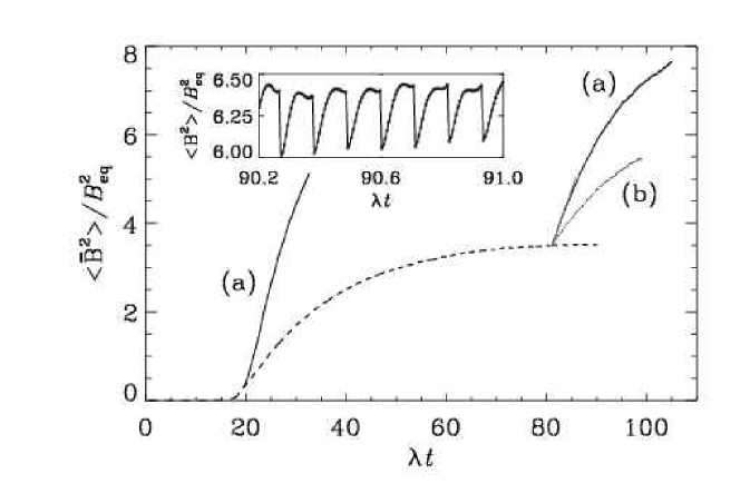
Figure 9.5: The effect of removing small scale magnetic energy in regular time intervals $\Delta t$ on the evolution of the large scale field (solid lines). The dashed line gives the evolution of $\langle\overline{\bm{B}}^{2}\rangle$ for Run 3 of Ref. [4], where no such energy removal was included. In all cases the field is shown in units of $B_{\rm eq}^{2}=\rho_{0}\langle\bm{u}^{2}\rangle$. The two solid lines show the evolution of $\langle\overline{\bm{B}}^{2}\rangle$ after restarting the simulation from Run 3 of Ref. [4] at $\lambda t=20$ and $\lambda t=80$. Time is scaled with the kinematic growth rate $\lambda$. The curves labeled (a) give the result for $\Delta t=0.12\lambda^{-1}$ and those labeled (b) for $\Delta t=0.4\lambda^{-1}$. The inset shows, for a short time interval, the sudden drop and subsequent recovery of the total (small and large scale) magnetic energy in regular time intervals. Adapted from [159].

In the experiment shown in Fig. 9.5 the flow is forced with helical waves at wavenumber $k=5$, giving rise to large scale dynamo action with slow saturation at wavenumber $k=1$. The magnetic field is then Fourier filtered in regular intervals (between a tenth and a quarter of the $e$-folding time of the kinematic dynamo) and the components above $k=4$ are set to zero, which is why this is called the vacuum cleaner experiment. Of course, the small scale magnetic energy will quickly recover and reach again equipartition field strength, but there remains a short time interval during which the small scale magnetic energy is in sub-equipartition, allowing the magnetic helicity to grow almost kinematically both at small and large scales. The effect from each such event is small, but the effect from all events together make up a sizeable enhancement to the amplitude of the generated large scale field.

9.6.4 Speculations about boundary conditions

In order for magnetic helicity losses to have an advantageous effect in the sun, or at least in a more realistic simulation, it is important that the losses of magnetic helicity occur predominantly at small scales. It is conceivable that preferentially small scale magnetic helicity losses may be possible in the presence of a more realistic modeling of the surface, where magnetostatic equilibrium configurations may lose stability, leading to the ejection of plasmoids and possibly magnetic helicity. In this context it is important to recall that, whenever magnetic eruptions of any form do occur, the field is always found to be strongly twisted [46, 47, 49, 409, 410]. It is therefore plausible that such events are an important part of the solar dynamo.

A second comment is here in order. Looking at the coronal mass ejections depicted in Fig. 2.3 it is clear that fairly large length scales are involved in this phenomenon. This makes the association with the small scale field dubious. Indeed, the division between large and small scale fields becomes exceedingly blurred, especially because small and large scale fields are probably associated with one and the same flux tube structure, as is clear from Fig. 9.6.

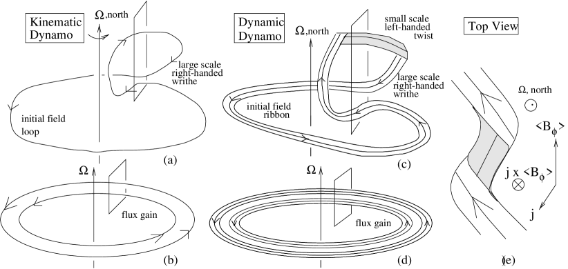
Figure 9.6: Schematic of kinematic helical $\alpha\Omega$ dynamo in northern hemisphere is shown in (a) and (b), whilst the dynamic helical $\alpha\Omega$ dynamo is shown by analogy in (c) and (d). Note that the mean field is represented as a line in (a) and (b) and as a tube in (c) and (d). (a) From an initial toroidal loop, the $\alpha$ effect induces a rising loop of right-handed writhe that gives a radial field component. (b) Differential rotation at the base of the loop shears the radial component, amplifying the toroidal component, and the ejection of the top part of loop (through coronal mass ejections) allow for a net flux gain through the rectangle. (c) Same as (a) but now with the field represented as a flux tube. This shows how the right-handed writhe of the large scale loop is accompanied by a left-handed twist along the tube, thus incorporating magnetic helicity conservation. (d) Same as (b) but with field represented as ribbon or tube. (e) Top view of the combined twist and writhe that can be compared with observed coronal magnetic structures in active regions. Note the N shape of the right-handed large scale twist in combination with the left-handed small scale twist along the tube. The backreaction force that resists the bending of the flux tube is seen to result from the small scale twist. Note that diffusing the top part of the loops both allows for net flux generation in the rectangles of (a)–(d), and alleviates the backreaction that could otherwise quench the dynamo. Courtesy E. G. Blackman [49].

Figure 9.7: Magnetic helicity spectra (scaled by wavenumber $k$ to give magnetic helicity per logarithmic interval) taken over the entire computational domain. The spectrum is dominated by a positive component at large scales ($k=1...5$) and a negative component at small scales ($k>5$). Adapted from Ref. [49].

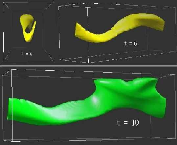
Figure 9.8: Three-dimensional visualization of a rising flux tube in the presence of rotation. The stratification is adiabatic such that temperature, pressure, and density all vanish at a height that is about 30% above the vertical extent shown. (The actual computational domain was actually larger in the $x$ and $z$ directions.) Adapted from Ref. [411].

The sketch shown in Fig. 9.6 shows another related aspect. Once a flux tube forms a twisted $\Omega$-shaped loop (via thermal or magnetic buoyancy) it develops a self-inflicted internal twist in the opposite sense. (In the sketch, which applies to the northern hemisphere, the tilt has positive sense, corresponding to positive writhe helicity, while the internal twist is negative.) These helicities can be associated with the positive $\overline{\mbox{\boldmath$J$}}\cdot\overline{\bm{B}}$ and the negative $\overline{\bm{j}\cdot\bm{b}}$, that has also been confirmed by calculating Fourier spectra from a buoyant flux tube tilting and twisting under the influence of the Coriolis force and the vertical density gradient [49, 411]; see Fig. 9.7. Instead of visualizing the magnetic field strength, which can be strongly affected by local stretching, we visualize the rising flux tube using a passive scalar field that was initially concentrated along the flux tube. This is shown in Fig. 9.8. This picture illustrates quite clearly that the $\alpha$ effect cannot operate without (at the same time) twist helicity of the opposite sign.

9.7 Effect of magnetic helicity losses on the $\alpha$ effect

An important problem associated with the dynamical quenching model, as formulated so far, is the fact that, unlike the volume average $\langle\overline{\mbox{\boldmath$A$}}\cdot\overline{\bm{B}}\rangle$ over a periodic domain, the spatially dependent magnetic helicity density $\overline{\bm{a}\cdot\bm{b}}$ is not gauge-invariant. First, it is possible to formulate the theory directly in terms of the small scale current helicity, $\overline{\bm{j}\cdot\bm{b}}$. We should note, however, that it is possible to define a gauge invariant magnetic helicity density for the small scale field as a density of correlated links and the associated flux [154]. We focus below on the formulation in terms of the current helicity density. Its evolution equation involves an extra divergence term or a current helicity flux, $\overline{\mbox{\boldmath${\cal F}$}}{}_{C}$. Using the evolution equation $\partial\bm{b}/\partial t=-\bm{\nabla}\times\bm{e}$, we can derive an evolution equation for the small scale current helicity in the form

$${\partial\over\partial t}\overline{\bm{j}\cdot\bm{b}}=-2\,\overline{\bm{e}\cdot\bm{c}}-\bm{\nabla}\cdot\overline{\mbox{\boldmath${\cal F}$}}{}_{C},$$ (9.55)

where $\bm{c}=\bm{\nabla}\times\bm{j}$ is the curl of the small scale current density, $\bm{j}=\bm{J}-\overline{\mbox{\boldmath$J$}}$, $\bm{e}=\bm{E}-\overline{\mbox{\boldmath$E$}}$ is the small scale electric field, $\overline{\mbox{\boldmath$E$}}=\eta\overline{\mbox{\boldmath$J$}}-\overline{\mbox{\boldmath${\mathcal{E}}$}}{}$ is the mean electric field, and

$$\overline{\mbox{\boldmath${\cal F}$}}{}_{C}=\overline{2\bm{e}\times\bm{j}}+\overline{(\bm{\nabla}\times\bm{e})\times\bm{b}}$$ (9.56)

is the mean current helicity flux resulting from the small scale field.

Mean-field models trying to incorporate such magnetic helicity fluxes have already been studied by Kleeorin and coworkers [394, 398, 399] in the context of both galactic and solar magnetic fields. An interesting flux of helicity which one obtains even in nonhelical but anisotropic turbulence due to the presence of shear has been pointed out by Vishniac and Cho [388]. The presence of such a flux in non-helical shearing turbulence has been confirmed numerically [412]. We will examine a general theory of such fluxes using the MTA in Section 10.4 below.

In the isotropic case, $\overline{\bm{e}\cdot\bm{c}}$ can be approximated by $k_{\rm f}^{2}\,\overline{\bm{e}\cdot\bm{b}}$. (Here we have assumed that the effect of triple correlation terms like $\overline{(\bm{u}\times\bm{b})\cdot\bm{\nabla}^{2}\bm{b}}$ in $\overline{\bm{e}\cdot\bm{c}}$ are small.) Using FOSA or MTA, this can be replaced by $k_{\rm f}^{2}(\overline{\mbox{\boldmath${\mathcal{E}}$}}{}\cdot\overline{\bm{B}}+\eta\overline{\bm{j}\cdot\bm{b}})$; see also Eq. (9.15), which then leads to the revised dynamical quenching formula

$${\partial\alpha\over\partial t}=-2\eta_{\rm t}k_{\rm f}^{2}\left({\alpha\overline{\bm{B}}^{2}-\eta_{\rm t}\overline{\mbox{\boldmath$J$}}\cdot\overline{\bm{B}}+{\textstyle{1\over 2}}k_{\rm f}^{-2}\bm{\nabla}\cdot\overline{\mbox{\boldmath${\cal F}$}}{}_{C}\over B_{\rm eq}^{2}}+{\alpha-\alpha_{\rm K}\over R_{\rm m}}\right),$$ (9.57)

where the current helicity flux, $\overline{\mbox{\boldmath${\cal F}$}}{}_{C}=2\overline{\bm{e}\times\bm{j}}+\overline{(\bm{\nabla}\times\bm{e})\times\bm{b}}$, has entered as an extra term in the dynamical quenching formula (9.15).

Making the adiabatic approximation, i.e. putting the RHS of Eq. (9.57) to zero, one arrives at the algebraic quenching formula

$$\alpha={\alpha_{\rm K}+R_{\rm m}\left(\eta_{\rm t}\overline{\mbox{\boldmath$J$}}\cdot\overline{\bm{B}}-{\textstyle{1\over 2}}k_{\rm f}^{-2}\bm{\nabla}\cdot\overline{\mbox{\boldmath${\cal F}$}}{}_{C}\right)/B_{\rm eq}^{2}\over 1+R_{\rm m}\overline{\bm{B}}^{2}/B_{\rm eq}^{2}}\quad\mbox{($\partial\alpha/\partial t=0$)}.$$ (9.58)

Considering again the $R_{\rm m}\to\infty$ limit, one has now

$$\alpha\to\eta_{\rm t}\tilde{k}_{\rm m}-{\textstyle{1\over 2}}k_{\rm f}^{-2}(\bm{\nabla}\cdot\overline{\mbox{\boldmath${\cal F}$}}{}_{C})/\overline{\bm{B}}^{2},$$ (9.59)

which shows that losses of negative helicity, as observed in the northern hemisphere of the sun, would enhance a positive $\alpha$ effect [394, 398, 399]. Here, $\tilde{k}_{\rm m}=\overline{\mbox{\boldmath$J$}}\cdot\overline{\bm{B}}/\overline{\bm{B}}^{2}$ is a spatially dependent generalization of Eq. (9.23) to the inhomogeneous case. If the current helicity flux is approximated by a Fickian diffusive flux proportional to the gradient of the small scale current helicity, i.e. $\overline{\mbox{\boldmath${\cal F}$}}{}_{C}\approx-2\eta_{\rm f}\bm{\nabla}\overline{\bm{j}\cdot\bm{b}}$, where $\eta_{\rm f}$ is an effective turbulent diffusion coefficient for the small scale current helicity (see Section 9.6.2), the second term of Eq. (9.59) becomes approximately $\eta_{\rm f}\tilde{k}_{\rm m}$, so $\alpha$ approaches a combination of $\eta_{\rm t}\tilde{k}_{\rm m}$ and $\eta_{\rm f}\tilde{k}_{\rm m}$, confirming again that $\alpha$ has increased.

In recent simulations with an imposed magnetic field [389], the dependence of $\alpha$ on the magnetic Reynolds number has been compared for both open and closed boundary conditions using the geometry depicted on the right hand panel of Fig. 9.9. As usual, $\alpha$ was determined by measuring the turbulent electromotive force, and hence $\alpha=\langle\mbox{\boldmath${\cal E}$}{}\rangle\cdot\bm{B}_{0}/B_{0}^{2}$. As expected, $\alpha$ is negative when the helicity of the forcing is positive, and $\alpha$ changes sign when the helicity of the forcing changes sign. The magnitudes of $\alpha$ are however different in the two cases: $|\alpha|$ is larger when the helicity of the forcing is negative. In the sun, this corresponds to the sign of helicity in the northern hemisphere in the upper parts of the convection zone. This is here the relevant case, because the differential rotation pattern of the present model also corresponds to the northern hemisphere.

Figure 9.9: Left: A sketch of the solar angular velocity at low latitudes with spoke-like contours in the bulk of the convection zone merging gradually into uniform rotation in the radiative interior. The low latitude region, modeled in this paper, is indicated by thick lines. Right: Differential rotation in our cartesian model, with the equator being at the bottom, the surface to the right, the bottom of the convection zone to the left and mid-latitudes at the top. Adapted from Ref. [389].

There is a striking difference between the cases with open and closed boundaries which becomes particularly clear when comparing the averaged values of $\alpha$ for different magnetic Reynolds numbers; see Fig. 9.10. With closed boundaries $\alpha$ tends to zero like $R_{\rm m}^{-1}$, while with open boundaries $\alpha$ shows no such decline. There is also a clear difference between the cases with and without shear, together with open boundaries in both cases. In the absence of shear (dashed line in Fig. 9.10) $\alpha$ declines with increasing $R_{\rm m}$, even though for small values of $R_{\rm m}$ it is larger than with shear.

Figure 9.10: Dependence of $|\langle\alpha\rangle|/u_{\rm rms}$ on $R_{\rm m}$ for open and closed boundaries. The case with open boundaries and negative helicity is shown as a dashed line. Note that for $R_{\rm m}\approx 30$ the $\alpha$ effect is about 30 times smaller when the boundaries are closed. The dotted line gives the result with open boundaries but no shear. The vertical lines indicate the range obtained by calculating $\alpha$ using only the first and second half of the time interval. Adapted from Ref. [389].

The difference between open and closed boundaries can be interpreted in terms of a current helicity flux through the two open boundaries of the domain. Inspections of the actual fluxes suggests that there is a tendency for the difference between incoming flux at the equator (dotted line) and outgoing fluxes at outer surface (solid line) to cancel, but the net outgoing flux is negative. The flux for the total field is approximately four times larger than what is accounted for by the Vishniac-Cho flux. This might indicate that there is either another contribution to the current helicity flux, or that the $\tau$ in the Vishniac-Cho flux is underestimated.

10 The microscopic theory of turbulent transport coefficients

In this section we describe in full detail the technique to calculate turbulent transport coefficients in the presence of slow rotation and weak inhomogeneity. The technique to incorporate slow rotation and weak inhomogeneity is the same as that introduced by Roberts and Soward [329] long ago, except that here we are using MTA. The present results are basically in full agreement with a recent calculation by Rädler, Kleeorin and Rogachevskii [320], except that here we retain the $\overline{\bm{j}\cdot\bm{b}}$ correction to $\alpha$ throughout, even when this term was vanishing initially. Indeed, in the nonlinear regime there is no limit in which this term can be ignored, because it is self-generated by the $\alpha$ effect. In this section, overbars denote ensemble averages, but for all practical purposes we may assume them to be equivalent to the spatial averages used before.

As we have emphasized before, the ignorance of the $\overline{\bm{j}\cdot\bm{b}}$ feedback term in much of the mean field dynamo literature is one of the main reasons why this theory has produced incorrect or unreliable results and has not been in agreement with numerical simulations of hydromagnetic turbulence [371]. We are now at a point where a lot of work has to be reconsidered with the correct feedback in place. What needs to be done now is a careful calculation of the turbulent transport coefficients that include, in particular, inhomogeneity and losses through boundaries. Here we are only able to present the initial steps in that direction.

10.1 Transport coefficients in weakly inhomogeneous turbulence

We consider the case when the correlation tensor of fluctuating quantities ($\bm{u}$ and $\bm{b}$) vary slowly on the system scale, say $\bm{R}$. Consider the equal time, ensemble average of the product $\overline{f(\bm{x}_{1})g(\bm{x}_{2})}$. The common dependence of $f$ and $g$ on $t$ is assumed and will not explicitly be stated. We have

$$\overline{f(\bm{x}_{1})g(\bm{x}_{2})}=\int\int\overline{\hat{f}(\bm{k}_{1})\hat{g}(\bm{k}_{2})}\e^{\mathrm{i}(\bm{k}_{1}\cdot\bm{x}_{1}+\bm{k}_{2}\cdot\bm{x}_{2})}\,\mathrm{d}^{3}k_{1}\ \mathrm{d}^{3}k_{2},$$ (10.1)

where $\hat{f}$ and $\hat{g}$ are the Fourier transforms of $f$ and $g$ respectively. (In general the Fourier transform of any function, say $f$, will be denoted by the same symbol with a ‘hat’ i.e. $\hat{f}$.) We define the difference $\bm{r}=\bm{x}_{1}-\bm{x}_{2}$ and the mean $\bm{R}={\textstyle{1\over 2}}(\bm{x}_{1}+\bm{x}_{2})$, keeping in mind that all two point correlations will vary rapidly with $\bm{r}$ but slowly with $\bm{R}$ [329]. We can re-express this correlation as

$$\overline{f(\bm{x}_{1})g(\bm{x}_{2})} = \int\int\overline{\hat{f}(\bm{k}+{\textstyle{1\over 2}}\bm{K})\hat{g}(-\bm{k}+{\textstyle{1\over 2}}\bm{K})}\ {\rm e}^{\mathrm{i}(\bm{K}\cdot\bm{R}+\bm{k}\cdot\bm{r})}\,\mathrm{d}^{3}K\ \mathrm{d}^{3}k$$ (10.2)

$$\equiv \int\Phi(\hat{f},\hat{g},\bm{k},\bm{R})\ {\rm e}^{i\bm{k}\cdot\bm{r}}\ \mathrm{d}^{3}k,$$

where we have defined the new wavevectors $\bm{k}={\textstyle{1\over 2}}(\bm{k}_{1}-\bm{k}_{2})$ and $\bm{K}=\bm{k}_{1}+\bm{k}_{2}$. Also for later convenience we define

$$\Phi(\hat{f},\hat{g},\bm{k},\bm{R})=\int\overline{\hat{f}(\bm{k}+{\textstyle{1\over 2}}\bm{K})\hat{g}(-\bm{k}+{\textstyle{1\over 2}}\bm{K})}\ {\rm e}^{i\bm{K}\cdot\bm{R}}\,\mathrm{d}^{3}K.$$ (10.3)

In what follows we require the correlation tensors of the $\bm{u}$ and $\bm{b}$ fields and the cross correlation between these two fields in Fourier space. The velocity and magnetic correlations, as well as the turbulent electromotive force $\overline{\mbox{\boldmath${\mathcal{E}}$}}{}$, are given by

$$v_{ij}(\bm{k},\bm{R}) = \Phi(\hat{u}_{i},\hat{u}_{j},\bm{k},\bm{R}),\quad\overline{\bm{u}^{2}}(\bm{R})=\delta_{ij}\int v_{ij}(\bm{k},\bm{R})\,\mathrm{d}^{3}k,$$ (10.4)

$$m_{ij}(\bm{k},\bm{R}) = \Phi(\hat{b}_{i},\hat{b}_{j},\bm{k},\bm{R}),\quad\overline{\bm{b}^{2}}(\bm{R})=\delta_{ij}\int m_{ij}(\bm{k},\bm{R})\,\mathrm{d}^{3}k,$$ (10.5)

$$\chi_{jk}(\bm{k},\bm{R}) = \Phi(\hat{u}_{j},\hat{b}_{k},\bm{k},\bm{R}),\quad\overline{\cal E}{}_{i}(\bm{R})=\epsilon_{ijk}\int\chi_{jk}(\bm{k},\bm{R})\,\mathrm{d}^{3}k.$$ (10.6)

In order to calculate these quantities we first consider the time derivative of $\chi_{jk}$,

$${\partial\chi_{jk}\over\partial t}=\Phi(\hat{u}_{j},\dot{\hat{b}_{k}},\bm{k},\bm{R})+\Phi(\dot{\hat{u}_{j}},\hat{b}_{k},\bm{k},\bm{R}),$$ (10.7)

where the dots on $\hat{b}_{j}$ and $\hat{u}_{i}$ denote a partial time derivative. The equation for $\bm{b}$ is given by Eq. (6.12). For the present we neglect the mean velocity term $\bm{U}$. The Fourier transform of this equation is then,

$$\dot{\hat{b}}_{k}(\bm{k})=\epsilon_{kpq}\epsilon_{qlm}\mathrm{i}k_{p}\int\hat{u}_{l}(\bm{k}-\bm{k}^{\prime})\hat{\overline{B}}_{m}(\bm{k}^{\prime})\,\mathrm{d}^{3}k^{\prime}+\hat{G}_{k}(\bm{k})-\eta k^{2}\hat{b}_{k}(\bm{k}),$$ (10.8)

where we have included the nonlinear term, $\bm{G}=\bm{\nabla}\times(\bm{u}\times\bm{b}-\overline{\bm{u}\times\bm{b}})$. (Note that since $\overline{\bm{u}\times\bm{b}}$ is a mean field quantity, it will give zero contribution to $\chi_{jk}$, when multiplied by $\hat{\mbox{$u$}}{}$ and ensemble averaged.) Using the momentum equation for the velocity field $\bm{U}$ and splitting the velocity into mean and fluctuating parts, $\bm{U}=\overline{\mbox{\boldmath$U$}}+\bm{u}$, and neglecting for simplicity the mean flow, $\overline{\mbox{\boldmath$U$}}=0$, we have, in a rotating frame,

$${\partial\bm{u}\over\partial t}=-\bm{\nabla}p_{\rm eff}+\overline{\bm{B}}\cdot\bm{\nabla}\bm{b}+\bm{b}\cdot\bm{\nabla}\overline{\bm{B}}-2\bm{\Omega}\times\bm{u}+\bm{H}+\bm{f}+\nu\bm{\nabla}^{2}\bm{u}.$$ (10.9)

Here we have assumed incompressible motions with $\bm{\nabla}\cdot\bm{u}=0$, and a constant density; we have therefore adopted units such that $\mu_{0}=\rho_{0}=1$. We have defined the effective pressure $p_{\rm eff}$ which contains the perturbed pressure including the magnetic contribution, $\bm{f}$ is the random external force, and the terms nonlinear in $\bm{u}$ and $\bm{b}$ are gathered in $\bm{H}=-\bm{u}\cdot\bm{\nabla}\bm{u}+\overline{\bm{u}\cdot\bm{\nabla}\bm{u}}+\bm{b}\cdot\bm{\nabla}\bm{b}-\overline{\bm{b}\cdot\bm{\nabla}\bm{b}}$. In the rotating frame, we also have a Coriolis force contribution $2\bm{\Omega}\times\bm{u}$. The effective pressure term can be obtained by solving a Poisson type equation derived by taking the divergence of Eq. (10.9). In Fourier space this corresponds to multiplying the equation by the projection operator, $P_{ij}(\bm{k})=\delta_{ij}-\hat{k}_{i}\hat{k}_{j}$, where $\hat{\bm{k}}=\bm{k}/|\bm{k}|$ is the unit vector of $\bm{k}$, so

$${\partial\hat{u}_{j}\over\partial t}=P_{js}\left[(\widehat{\overline{\bm{B}}\cdot\bm{\nabla}\bm{b}})_{s}+(\widehat{\bm{b}\cdot\bm{\nabla}\overline{\bm{B}}})_{s}-2\epsilon_{slm}\Omega_{l}\hat{u}_{m}+\hat{f}_{s}+\hat{H}_{s}-\nu k^{2}\hat{u}_{s}\right].$$ (10.10)

Here we have dropped the argument $\bm{k}$ on all quantities and, for brevity, we have introduced the notation

$$(\widehat{\overline{\bm{B}}\cdot\bm{\nabla}\bm{b}})_{s}=\int\hat{\overline{B}}_{l}(\bm{k}-\bm{k}^{\prime})(\mathrm{i}k^{\prime}_{l})\,\hat{b}_{s}(\bm{k}^{\prime})\,\mathrm{d}^{3}k^{\prime},$$ (10.11)

$$(\widehat{\bm{b}\cdot\bm{\nabla}\overline{\bm{B}}})_{s}=\int\hat{b}_{l}(\bm{k}-\bm{k}^{\prime})(\mathrm{i}k^{\prime}_{l})\,\hat{\overline{B}}_{s}(\bm{k}^{\prime})\,\mathrm{d}^{3}k^{\prime}$$ (10.12)

for the Fourier transforms of the magnetic tension/curvature force. We can simplify the rotational part of the Coriolis force by using the identity

$$\epsilon_{ijk}=\hat{k}_{i}\hat{k}_{p}\epsilon_{pjk}+\hat{k}_{j}\hat{k}_{p}\epsilon_{ipk}+\hat{k}_{k}\hat{k}_{p}\epsilon_{ijp},$$ (10.13)

noting that $P_{ij}\epsilon_{jkl}=\hat{k}_{k}\hat{k}_{p}\epsilon_{ipl}+\hat{k}_{l}\hat{k}_{p}\epsilon_{ikp}$, and using incompressibility $\hat{k}_{k}\hat{u}_{k}=0$, to get

$$P_{js}(\bm{k})\,\epsilon_{slm}\Omega_{l}\hat{u}_{m}=\hat{\bm{k}}\cdot\bm{\Omega}\,\epsilon_{jpm}\hat{k}_{p}\hat{u}_{m}.$$ (10.14)

We are now in a position to calculate $\partial\chi_{jk}/\partial t$. Using the induction equation for $\dot{\hat{\bm{b}}}$ given by (10.8), the first term in (10.7) is given by

$$\Phi(\hat{u}_{j},\dot{\hat{b}_{k}},\bm{k},\bm{R})=\dot{\chi}_{jk}^{\rm K}+\overline{\hat{\mbox{$u$}}{}_{j}\hat{\mbox{$G$}}{}_{k}}-\eta(\bm{k}+{\textstyle{1\over 2}}\mathrm{i}\bm{\nabla})^{2}\chi_{jk},$$ (10.15)

where we have substituted $\bm{K}$ by $-\mathrm{i}\bm{\nabla}$ and have introduced the abbreviation

$$\dot{\chi}_{jk}^{\rm K}=\epsilon_{kpq}\epsilon_{qlm} \int \overline{\hat{\mbox{$u$}}{}_{j}(\bm{k}+{\textstyle{1\over 2}}\bm{K})\hat{\mbox{$u$}}{}_{l}(-\bm{k}+{\textstyle{1\over 2}}\bm{K}-\bm{k}^{\prime})}\,\hat{\overline{\mbox{$B$}}}{}_{m}(\bm{k}^{\prime})$$ (10.16)

$$\times \mathrm{i}(-k_{p}+{\textstyle{1\over 2}}K_{p})\ \mathrm{d}^{3}k^{\prime}\e^{\mathrm{i}\bm{K}\cdot\bm{R}}\ \mathrm{d}^{3}K.$$

Further the triple correlations of the form $\overline{\hat{\mbox{$u$}}{}_{j}\hat{\mbox{$G$}}{}_{k}}$, will be either ignored (FOSA) or replaced by the double correlation $\chi_{jk}$, divided by a relaxation time (the $\tau$ approximation). To evaluate the above velocity correlation in $\partial\chi_{jk}^{K}/\partial t$, we need to bring the $\overline{\hat{\mbox{$u$}}{}_{j}\hat{\mbox{$u$}}{}_{l}}$ term into a form similar to Eq. (10.4), so that we can replace it by $v_{jl}$. Thus, we define new wavevectors $\bm{k}_{1}=\bm{k}+{\textstyle{1\over 2}}\bm{K}$ and $\bm{k}_{2}=-\bm{k}+{\textstyle{1\over 2}}\bm{K}+\bm{k}^{\prime}$, and transform to new variables, ($\bm{k}^{\prime},\bm{K}^{\prime}$), where $\bm{K}^{\prime}=\bm{k}_{1}+\bm{k}_{2}=\bm{K}-\bm{k}^{\prime}$. We then have

$$\dot{\chi}_{jk}^{\rm K}=\epsilon_{kpq}\epsilon_{qlm} \int \overline{\hat{\mbox{$u$}}{}_{j}(\bm{k}+{\textstyle{1\over 2}}\bm{k}^{\prime}+{\textstyle{1\over 2}}\bm{K}^{\prime})\,\hat{\mbox{$u$}}{}_{l}(-(\bm{k}+{\textstyle{1\over 2}}\bm{k}^{\prime})+{\textstyle{1\over 2}}\bm{K}^{\prime})}\hat{\overline{\mbox{$B$}}}{}_{m}(\bm{k}^{\prime})$$ (10.17)

$$\mathrm{i}(-k_{p}+{\textstyle{1\over 2}}k^{\prime}_{p}+{\textstyle{1\over 2}}K^{\prime}_{p})\ \e^{\mathrm{i}(\bm{K}^{\prime}+\bm{k}^{\prime})\cdot\bm{R}}\ \mathrm{d}^{3}K^{\prime}\ \mathrm{d}^{3}k^{\prime}.$$

Using the definition of the velocity correlation function $v_{ij}$ in Eqs. (10.3) and (10.4) and carrying out first the integral over $\bm{K}^{\prime}$, and replace $\mathrm{i}K^{\prime}_{p}$ by $\nabla_{p}\equiv\partial/\partial R_{p}$, we can write

$$\dot{\chi}_{jk}^{\rm K}=\epsilon_{kpq}\epsilon_{qlm}\int(-\mathrm{i}k_{p}+{\textstyle{1\over 2}}\mathrm{i}k^{\prime}_{p}+{\textstyle{1\over 2}}\nabla_{p})\,v_{jl}(\bm{k}+{\textstyle{1\over 2}}\bm{k}^{\prime},\bm{R})\hat{\overline{\mbox{$B$}}}{}_{m}(\bm{k}^{\prime})\e^{\mathrm{i}\bm{k}^{\prime}\cdot\bm{R}}\mathrm{d}^{3}k^{\prime}.$$ (10.18)

Note that, since the mean field $\overline{\bm{B}}$ varies only on large scales, $\hat{\overline{\mbox{$B$}}}{}(\bm{k}^{\prime})$ will be non-zero only for small $\mid\!\!\bm{k}^{\prime}\!\!\mid$. This suggests expanding $v_{jl}$ above in a Taylor series in $\bm{k}^{\prime}$, i.e.

$$v_{jl}(\bm{k}+{\textstyle{1\over 2}}\bm{k}^{\prime},\bm{R})\approx v_{jl}(\bm{k},\bm{R})+{\textstyle{1\over 2}}k^{\prime}_{s}{\partial\over\partial k_{s}}v_{jl}(\bm{k},\bm{R}).$$ (10.19)

We will keep only terms that can contribute derivatives in $\bm{R}$ no higher than the first derivative. Integrating over $\bm{k}^{\prime}$, using $\epsilon_{kpq}\epsilon_{qlm}=\delta_{kl}\delta_{pm}-\delta_{km}\delta_{pl}$, and noting that the inverse Fourier transform of $\mathrm{i}k_{s}^{\prime}\hat{\overline{\mbox{$B$}}}{}_{m}(\bm{k}^{\prime})$ is $\overline{B}_{m,s}\equiv\partial\overline{B}_{m}/\partial R_{s}$, we get

$$\dot{\chi}_{jk}^{\rm K}=-\mathrm{i}\bm{k}\cdot\overline{\bm{B}}\,v_{jk}+{\textstyle{1\over 2}}\overline{\bm{B}}\cdot\bm{\nabla}v_{jk}-v_{jl}{\partial\overline{B}_{k}\over\partial R_{l}}-{\textstyle{1\over 2}}k_{m}{\partial v_{jk}\over\partial k_{s}}\overline{B}_{m,s}.$$ (10.20)

Now turn to the second term in (10.7) for $\partial\chi_{jk}/\partial t$. This is given by

$$\Phi(\dot{\hat{u}_{j}},\hat{b}_{k},\bm{k},\bm{R})=\dot{\chi}_{jk}^{\rm M}+\dot{\chi}_{jk}^{\Omega}+\overline{\hat{\mbox{$H$}}{}_{j}\hat{\mbox{$b$}}{}_{k}}-\nu(\bm{k}-{\textstyle{1\over 2}}\mathrm{i}\bm{\nabla})^{2}\chi_{jk},$$ (10.21)

where

$$\dot{\chi}_{jk}^{\rm M} = \int\ \mathrm{d}^{3}k^{\prime}\ \mathrm{d}^{3}K\e^{\mathrm{i}\bm{K}\cdot\bm{R}}\ P_{js}(\bm{k}+{\textstyle{1\over 2}}\bm{K})\times$$ (10.22)

$$[\mathrm{i}(k_{l}+{\textstyle{1\over 2}}K_{l}-k^{\prime}_{l})\ \hat{\overline{\mbox{$B$}}}{}_{l}(\bm{k}^{\prime})\ \overline{\hat{\mbox{$b$}}{}_{s}(\bm{k}+{\textstyle{1\over 2}}\bm{K}-\bm{k}^{\prime})\hat{\mbox{$b$}}{}_{k}(-\bm{k}+{\textstyle{1\over 2}}\bm{K})}$$

$$+ (\mathrm{i}k^{\prime}_{l})\ \hat{\overline{\mbox{$B$}}}{}_{s}(\bm{k}^{\prime})\ \overline{\hat{\mbox{$b$}}{}_{l}(\bm{k}+{\textstyle{1\over 2}}\bm{K}-\bm{k}^{\prime})\hat{\mbox{$b$}}{}_{k}(-\bm{k}+{\textstyle{1\over 2}}\bm{K})}],$$

and

$$\dot{\chi}_{jk}^{\Omega}=2\Omega_{m}\epsilon_{jlt}\int{p_{m}p_{t}\over\bm{p}^{2}}\,\overline{\hat{\mbox{$u$}}{}_{l}(\bm{k}+{\textstyle{1\over 2}}\bm{K})\hat{\mbox{$b$}}{}_{k}(-\bm{k}+{\textstyle{1\over 2}}\bm{K})}\e^{\mathrm{i}\bm{K}\cdot\bm{R}}\ \mathrm{d}^{3}K.$$ (10.23)

Here we have introduced $\bm{p}=\bm{k}+{\textstyle{1\over 2}}\bm{K}$ for brevity. Once again, the triple correlations of the form $\overline{\hat{\mbox{$H$}}{}_{j}\hat{\mbox{$b$}}{}_{k}}$, will be either ignored (FOSA) or replaced by the double correlation $\chi_{jk}$, divided by a typical correlation time (the $\tau$ approximation). Empirically, we know that the term $\overline{\hat{\bm{f}}\cdot\hat{\bm{b}}}$ is small. We first simplify the $\dot{\chi}_{jk}^{\Omega}$ term, keeping only terms that are at most a first derivative in $\bm{R}$. For this first expand $p_{m}p_{t}/\bm{p}^{2}$ as

$${(k_{m}+{\textstyle{1\over 2}}K_{m})(k_{t}+{\textstyle{1\over 2}}K_{t})\over(\bm{k}+{\textstyle{1\over 2}}\bm{K})^{2}}={k_{m}k_{t}\over k^{2}}+{k_{m}K_{t}\over 2k^{2}}+{K_{m}k_{t}\over 2k^{2}}-{k_{m}k_{t}k_{s}K_{s}\over k^{4}},$$ (10.24)

keeping terms that are at most linear in $\bm{K}$. Then the integral over $\bm{K}$ can be carried out using the definition of $\chi_{ij}$. We get

$$\dot{\chi}_{jk}^{\Omega}=-{\sf A}_{jl}\chi_{lk}-{\sf B}_{jlm}{\partial\chi_{lk}\over\partial R_{m}},$$ (10.25)

where the $\chi_{lk}$ without superscript is the full $\chi_{lk}$, and

$${\sf A}_{jl}=-2\epsilon_{jlt}{\bm{k}\cdot\bm{\Omega}\over k^{2}}k_{t},$$ (10.26)

$${\sf B}_{jlm}=\mathrm{i}\epsilon_{jlm}{\bm{k}\cdot\bm{\Omega}\over k^{2}}+\mathrm{i}\epsilon_{jlt}{k_{t}\Omega_{m}\over k^{2}}-2\mathrm{i}\epsilon_{jlt}{(\bm{k}\cdot\bm{\Omega})k_{t}k_{m}\over k^{4}}.$$ (10.27)

As shown in Appendix E, the simplification of $\dot{\chi}_{jk}^{\rm M}$ leads to

$$\dot{\chi}_{jk}^{\rm M} = \mathrm{i}\bm{k}\cdot\overline{\bm{B}}\,m_{jk}+{\textstyle{1\over 2}}\overline{\bm{B}}\cdot\bm{\nabla}m_{jk}+\overline{B}_{j,l}m_{lk}$$ (10.28)

$$- {\textstyle{1\over 2}}\overline{B}_{m,s}k_{m}{\partial m_{jk}\over\partial k_{s}}-2{k_{j}k_{s}\over k^{2}}\overline{B}_{s,l}m_{lk}.$$

We can now add all the different contributions to get,

$${\partial\chi_{jk}\over\partial t}={\sf I}_{jk}- {\sf A}_{jl}\chi_{lk}-{\sf B}_{jlm}{\partial\chi_{lk}\over\partial R_{m}}$$ (10.29)

$$+\overline{\hat{\mbox{$u$}}{}_{j}\hat{\mbox{$G$}}{}_{k}}+\overline{\hat{\mbox{$H$}}{}_{j}\hat{\mbox{$b$}}{}_{k}}-(\eta+\nu)k^{2}\chi_{jk}-\mathrm{i}(\eta-\nu)\bm{k}\cdot\bm{\nabla}\chi_{jk},$$

where

$${\sf I}_{jk} = -\mathrm{i}\bm{k}\cdot\overline{\bm{B}}\,(v_{jk}-m_{jk})+{\textstyle{1\over 2}}\overline{\bm{B}}\cdot\bm{\nabla}(v_{jk}+m_{jk})+\overline{B}_{j,l}m_{lk}-\overline{B}_{k,l}v_{jl}$$ (10.30)

$$- {\textstyle{1\over 2}}\overline{B}_{m,s}k_{m}\left[{\partial v_{jk}\over\partial k_{s}}+{\partial m_{jk}\over\partial k_{s}}\right]-2{k_{j}k_{s}\over k^{2}}\overline{B}_{s,l}m_{lk},$$

and we have only kept the terms in the microscopic diffusion and viscosity up to first order in the large scale derivative.

The first order smoothing approximation can be recovered by neglecting the triple correlation terms $\langle\hat{\mbox{$u$}}{}_{j}\hat{\mbox{$G$}}{}_{k}\rangle+\langle\hat{\mbox{$H$}}{}_{j}\hat{\mbox{$b$}}{}_{k}\rangle$. Using MTA, one summarily approximates the triple correlations as a damping term, and takes $\langle\hat{\mbox{$u$}}{}_{j}\hat{\mbox{$G$}}{}_{k}\rangle+\langle\hat{\mbox{$H$}}{}_{j}\hat{\mbox{$b$}}{}_{k}\rangle\approx-\chi_{jk}/\tau(k)$, where in general the parameter $\tau$ could be $k$-dependent. (The microscopic diffusion terms can either be absorbed into the definition of $\tau(k)$ or neglected for large Reynolds numbers.) One then has

$${\partial\chi_{jk}\over\partial t}={\sf I}_{jk}-{\sf A}_{jl}\chi_{lk}-{\sf B}_{jlm}{\partial\chi_{lk}\over\partial R_{m}}-{\chi_{jk}\over\tau},$$ (10.31)

or

$${\partial\chi_{jk}\over\partial t}={\sf I}_{jk}-{1\over\tau}{\sf D}_{jl}\chi_{lk}-{\sf B}_{jlm}{\partial\chi_{lk}\over\partial R_{m}},$$ (10.32)

where ${\sf D}_{jl}=\delta_{jl}+\tau{\sf A}_{jl}$. On time scales long compared with $\tau$, one can neglect the time derivative of $\chi_{jk}$, so one has [8]

$${\sf D}_{jl}\chi_{lk}+\tau{\sf B}_{jlm}{\partial\chi_{lk}\over\partial R_{m}}=\tau{\sf I}_{jk}.$$ (10.33)

In the weakly inhomogeneous case that we are considering, this equation can be solved iteratively. To zeroth order, one neglects the $\partial/\partial\bm{R}$ terms on both sides of Eq. (10.33). This gives a zeroth order estimate

$$\chi_{lk}^{(0)}={\sf D}^{-1}_{lj}\,\tau{\sf I}_{jk}^{(0)},$$ (10.34)

where

$${\sf I}_{jk}^{(0)}=-\mathrm{i}\bm{k}\cdot\overline{\bm{B}}\,(v_{jk}-m_{jk}).$$ (10.35)

Here the inverse matrix ${\sf D}_{jl}^{-1}$ is given by

$${\sf D}_{jl}^{-1}=\left.\left(\delta_{jl}+\mbox{\rm Co}_{\bm{k}}\epsilon_{jlm}\hat{k}_{m}+\mbox{\rm Co}_{\bm{k}}^{2}\hat{k}_{j}\hat{k}_{l}\right)\right/\left(1+\mbox{\rm Co}_{\bm{k}}^{2}\right),$$ (10.36)

where $\mbox{\rm Co}_{\bm{k}}\equiv 2\bm{\Omega}\tau\cdot\hat{\bm{k}}$ is the Coriolis number with respect to the component of $\bm{\Omega}$ that is aligned with $\bm{k}$, and $\hat{\bm{k}}\equiv\bm{k}/k$ is the unit vector of $\hat{\bm{k}}$.

To the next order, we keep first derivative terms and substitute $\chi_{lk}^{(0)}$ in the $\partial\chi_{lk}/\partial R_{m}$ term. This gives

$$\chi_{jk}={\sf D}_{jl}^{-1}\tau{\sf I}_{lk}-\tau^{2}{\sf D}^{-1}_{jp}{\sf B}_{plm}{\partial\over\partial R_{m}}\left({\sf D}^{-1}_{ls}{\sf I}_{sk}^{(0)}\right).$$ (10.37)

Further, in many situations one will be concerned with the slow rotation limit, where $\Omega\tau\ll 1$. In this case one needs to keep only terms that are at most linear in $\Omega\tau$. We do this below; partial results to higher order in $\Omega\tau$ can be found in Ref. [320]. To linear order, ${\sf D}_{jl}^{-1}=\delta_{jl}+2\tau\hat{\bm{k}}\cdot\bm{\Omega}\epsilon_{jlm}\hat{k}_{m}$. Substituting this into Eq. (10.37), and noting that the ${\sf B}_{plm}$ term is already linear in $\Omega$, we get

$$\chi_{jk}=\tau{\sf I}_{jk}+2\tau^{2}\hat{\bm{k}}\cdot\bm{\Omega}\epsilon_{jlm}\hat{k}_{m}{\sf I}_{lk}-\tau^{2}{\sf B}_{jlm}{\partial{\sf I}_{lk}^{(0)}\over\partial R_{m}}.$$ (10.38)

We will work with this expression to evaluate $\overline{\mbox{\boldmath${\mathcal{E}}$}}{}$. The first term in (10.38) contributes to $\overline{\mbox{\boldmath${\mathcal{E}}$}}{}$, even in the case when $\Omega=0$. This contribution is given by

$$\overline{\mbox{\boldmath${\mathcal{E}}$}}{}^{(0)}_{i} = \epsilon_{ijk}\int\tau{\sf I}_{jk}\,\mathrm{d}^{3}k$$

$$= \epsilon_{ijk}\int\tau\Big{[}-\mathrm{i}\bm{k}\cdot\overline{\bm{B}}(v_{jk}^{\rm A}-m_{jk}^{\rm A})+{\textstyle{1\over 2}}\overline{\bm{B}}\cdot\bm{\nabla}(v_{jk}^{\rm A}+m_{jk}^{\rm A})$$

$$+ \overline{B}_{j,l}m_{lk}-\overline{B}_{k,l}v_{jl}-{\textstyle{1\over 2}}k_{m}\ \overline{B}_{m,s}\left({\partial v_{jk}^{\rm A}\over\partial k_{s}}+{\partial m_{jk}^{\rm A}\over\partial k_{s}}\right)-2{k_{j}k_{s}\over k^{2}}\overline{B}_{s,l}m_{lk}\Big{]}\mathrm{d}^{3}k.$$

Note that due to the presence of the antisymmetric tensor $\epsilon_{ijk}$ only the antisymmetric parts of $v_{jk}$ and $m_{jk}$ survive in some of the terms above, and these are denoted by $v_{jk}^{\rm A}$ and $m_{jk}^{\rm A}$, respectively.

To proceed we need the form of the velocity and magnetic correlation tensors. We adopt the form relevant when these are isotropic and weakly inhomogeneous, as discussed in detail in Refs [320, 329]. We take

$$v_{ij} = \left[P_{ij}(\bm{k})+{\mathrm{i}\over 2k^{2}}(k_{i}\nabla_{j}-k_{j}\nabla_{i})\right]E(k,\bm{R})$$ (10.40)

$$- {1\over 2k^{2}}\left[\epsilon_{ijk}k_{k}\left(2\mathrm{i}+\!{\bm{k}\cdot\bm{\nabla}\over k^{2}}\right)-(k_{i}\epsilon_{jlm}\!+\!k_{j}\epsilon_{ilm}){k_{l}\over k^{2}}\nabla_{m}\right]F(k,\bm{R}),$$

$$m_{ij} = \left[P_{ij}(\bm{k})+{\mathrm{i}\over 2k^{2}}(k_{i}\nabla_{j}-k_{j}\nabla_{i})\right]M(k,\bm{R})$$ (10.41)

$$- {1\over 2k^{2}}\left[\epsilon_{ijk}k_{k}\left(2\mathrm{i}+\!{\bm{k}\cdot\bm{\nabla}\over k^{2}}\right)-(k_{i}\epsilon_{jlm}\!+\!k_{j}\epsilon_{ilm}){k_{l}\over k^{2}}\nabla_{m}\right]N(k,\bm{R}).$$

Here $4\pi k^{2}E$ and $4\pi k^{2}M$ are the kinetic and magnetic energy spectra, respectively, and $4\pi k^{2}F$ and $4\pi k^{2}N$ are the corresponding helicity spectra. (Note that in this section we use the symbol $F(k,\bm{R})$ to denote the kinetic helicity spectrum; this should not be confused with the the coordinate space $F(r)$ defined earlier, for the helical part of the velocity correlation function.) They obey the relations

$$\overline{\bm{u}^{2}}\left(\bm{R}\right)=2\int E(k,\bm{R})\,\mathrm{d}^{3}k,\quad\overline{\bm{\omega}\cdot\bm{u}}\left(\bm{R}\right)=2\int F(k,\bm{R})\,\mathrm{d}^{3}k,$$

$$\overline{\bm{b}^{2}}\left(\bm{R}\right)=2\int M(k,\bm{R})\,\mathrm{d}^{3}k,\quad\overline{\bm{j}\cdot\bm{b}}\left(\bm{R}\right)=2\int N(k,\bm{R})\,\mathrm{d}^{3}k.$$ (10.42)

Note that, so far, we have also made no assumptions about the origin of the velocity and magnetic fluctuations, apart from their general form. The fluctuating velocity could be driven by random forcing and also be responding to the effects of rotation and/or the nonlinear effects of the Lorentz forces. For example, suppose one were to assume that the turbulence were originally nonhelical, that is $E=E^{(0)}$ and $F$ was originally zero. The helical parts of the velocity correlations can still be generated due to rotation and stratification. In this case the helical part of the velocity correlation will no longer be isotropic, and will reflect the anisotropy induced by both rotation and stratification. To work out the corresponding modification to $v_{ij}$ one has to take into account the effect of the Coriolis force in some approximate way. This has been done in Ref. [329] by assuming that the velocity induced by rotation is very small compared to the original turbulent velocity and using the $\tau$ approximation in [320]. Interestingly, it turns out that, to the lowest order in $R$ derivatives, rotation induces a helical part to $v_{ij}$ that can be described simply by adopting an anisotropic $F=F^{\Omega}$. It is shown in Ref. [320] that, under the $\tau$ approximation, this is given by

$$F^{\Omega}(\bm{k},\bm{R})=-2\tau^{*}\left[(\hat{\bm{k}}\cdot\bm{\Omega})\,(\hat{\bm{k}}\cdot\bm{\nabla})-\bm{\Omega}\cdot\bm{\nabla}\right]E^{(0)}(k,\bm{R}),$$ (10.43)

where $\tau^{*}(k)$ is another correlation time, that could in principle be different from $\tau(k)$. We use this for $F$ when we discuss the effects of rotation, although one must keep in mind that it is likely to give only a crude and at most qualitative estimate of the effects of rotation.

We substitute the velocity and magnetic correlations given in (10.40) and (10.41) into (10.1) for $\overline{\mbox{\boldmath${\mathcal{E}}$}}{}^{(0)}$. Note that the term proportional to $v_{jk}^{\rm A}+m_{jk}^{\rm A}$ gives zero contribution, as the antisymmetric parts of the correlations are odd in $k_{i}$ and so integrate to zero, while doing the $k$-integration. (This continues to hold even if $F=F^{\Omega}$.) Also the terms that have $k$ derivatives, give zero contribution after integrating by parts, and using $\bm{\nabla}\cdot\overline{\bm{B}}=0$. Further, in terms which already have $R_{i}$ derivatives of $\overline{\bm{B}}$, one need not include the $R_{i}$ derivative contributions of $v_{jk}$ and $m_{jk}$. The remaining terms can be written as

$$\overline{\mbox{\boldmath${\mathcal{E}}$}}{}^{(0)}_{i} = \epsilon_{ijk}\int\tau\Big{\{}\hat{\bm{k}}\cdot\overline{\bm{B}}\left[{\textstyle{1\over 2}}(\hat{\mbox{$k$}}{}_{j}\nabla_{k}-\hat{\mbox{$k$}}{}_{k}\nabla_{j})(E-M)-\epsilon_{jkm}\hat{\mbox{$k$}}{}_{m}(F-N)\right]$$ (10.44)

$$+ \overline{B}_{j,l}P_{lk}(\bm{k})M-\overline{B}_{k,l}P_{jl}(\bm{k})E-2\hat{\mbox{$k$}}{}_{j}\hat{\mbox{$k$}}{}_{s}\overline{B}_{s,l}P_{lk}(\bm{k})M\Big{\}}\,\mathrm{d}^{3}k,$$

where, as before, commas denote partial differentiation with respect to $R$, i.e. $\overline{B}_{j,l}\equiv\partial\overline{B}_{j}/\partial R_{l}$.

10.2 Isotropic, helical, nonrotating turbulence

In the first instance, suppose we were to assume that the turbulence is driven by isotropic forcing which is also helical, so that all spectral functions depend only on $\mid\!\!\bm{k}\!\!\mid$. One can then do the angular parts of the $k$-integral in (10.44), using a relation valid for any ${\cal F}(k)$ of the form

$$\int\hat{\mbox{$k$}}{}_{i}\hat{\mbox{$k$}}{}_{j}{\cal F}(k)\,\mathrm{d}^{3}k={\textstyle{1\over 3}}\delta_{ij}\int{\cal F}(k)\,\mathrm{d}^{3}k.$$ (10.45)

We get

$$\overline{\mbox{\boldmath${\mathcal{E}}$}}{}^{(0)}_{i}=\epsilon_{ijk}\left[(\overline{B}_{j}\nabla_{k}-\overline{B}_{k}\nabla_{j}){\tilde{E}-\tilde{M}\over 6}-\epsilon_{jkm}\overline{B}_{m}{\tilde{F}-\tilde{N}\over 3}-{\textstyle{2\over 3}}\overline{B}_{k,j}\tilde{E}\right],$$ (10.46)

where we have defined

$$\tilde{E}=\int\tau(k)E(k,\bm{R})\,\mathrm{d}^{3}k,\quad\tilde{M}=\int\tau(k)M(k,\bm{R})\,\mathrm{d}^{3}k,$$

$$\tilde{F}=\int\tau(k)F(k,\bm{R})\,\mathrm{d}^{3}k,\quad\tilde{N}=\int\tau(k)N(k,\bm{R})\,\mathrm{d}^{3}k.$$ (10.47)

For a constant $\tau(k)=\tau_{0}$ say, we simply have $\tilde{E}={\textstyle{1\over 2}}\tau_{0}\overline{\bm{u}^{2}}$, $\tilde{M}={\textstyle{1\over 2}}\tau_{0}\overline{\bm{b}^{2}}$, $\tilde{F}={\textstyle{1\over 2}}\tau_{0}\overline{\bm{\omega}\cdot\bm{u}}$, $\tilde{N}={\textstyle{1\over 2}}\tau_{0}\overline{\bm{j}\cdot\bm{b}}$. In this case we have for the turbulent EMF

$$\overline{\mbox{\boldmath${\mathcal{E}}$}}{}^{(0)}=\alpha\overline{\bm{B}}-\eta_{\rm t}\overline{\mbox{\boldmath$J$}}+\bm{\gamma}\times\overline{\bm{B}},$$ (10.48)

where

$$\alpha=-{\textstyle{1\over 3}}\tau_{0}(\overline{\bm{\omega}\cdot\bm{u}}-\overline{\bm{j}\cdot\bm{b}}),\quad\eta_{\rm t}={\textstyle{1\over 3}}\tau_{0}\overline{\bm{u}^{2}},\quad\bm{\gamma}=-{\textstyle{1\over 6}}\tau_{0}\bm{\nabla}(\overline{\bm{u}^{2}}-\overline{\bm{b}^{2}}),$$ (10.49)

and $\mu_{0}=\rho_{0}=1$ is still assumed. We see that the $\alpha$ effect has the advertised current helicity correction, but the turbulent diffusion is unaffected by the small scale magnetic fluctuations. There is also a turbulent diamagnetic effect and this is affected by magnetic fluctuations, vanishing for equipartition fields. We should also point out that the fluctuating velocity and magnetic fields above are the actual fields and not that of some fiducial ‘original’ turbulence as for example implied in [320]. Of course, we have not calculated what the values of $\overline{\bm{\omega}\cdot\bm{u}}$, $\overline{\bm{j}\cdot\bm{b}}$, etc are; one possibility is to take them from a turbulence simulations.

Note also that assuming $\tau$ independent of $k$ may be adequate if the magnetic and kinetic spectra are dominated by a single scale. However, it can be misleading if $F$ and $N$ are non zero over a range of scales. In such a case it is better to adopt a physically motivated $\tau(k)$. For example if the turbulence is maximally helical and $F(k)\propto kE(k)$, with $E(k)\propto k^{-11/3}$ as in Kolmogorov turbulence, then $\tau_{0}\int F(k)\,\mathrm{d}k\propto\int kk^{-5/3}\mathrm{d}k$ would be dominated by the smallest scale and the kinetic and magnetic $\alpha$ effects will be Reynolds number dependent. However, if one takes for $\tau(k)\propto k^{-2/3}$ the eddy turnover time in Kolmogorov turbulence, then $\int\tau(k)F(k)\,\mathrm{d}^{3}k\propto k^{-1/3}$ and the $\alpha$ effects (both kinetic and magnetic) would be determined by the kinetic/current helicities at the forcing scale of the turbulence and independent of Reynolds number. It is important to keep this feature in mind in interpreting expressions with constant $\tau_{0}$. (We thank Dmitry Sokoloff for this suggestion.) We note, however, that recent simulations at higher resolution (up to $512^{3}$ meshpoints) indicate that the small scale velocity and magnetic fields are no longer fully helical beyond the forcing wavenumber [327]. Thus, the spectra of kinetic and current helicities scale approximately like $k^{-5/3}$.

10.3 Turbulence with helicity induced by rotation

Now consider the case when helicity in the turbulence is induced by rotation and stratification. For this case, we adopt a velocity correlation function, where $F$ is related to $E$ as in (10.43). For $m_{jk}$, we retain the expression given by (10.41). Note that in Ref. [320] the current helicity terms have been neglected in the calculation of the effects of rotation on $\overline{\mbox{\boldmath${\mathcal{E}}$}}{}$. There is no reason to make this assumption, as even if such helical magnetic correlations were initially zero, they would be generated dynamically, during the operation of the large scale dynamo due to magnetic helicity conservation. So we have to keep this term as well. We will also only keep terms linear in $\Omega\tau$ and linear in the $R_{i}$ derivative.

The first term in (10.38) also gives now an $\Omega$ dependent contribution to $\overline{\mbox{\boldmath${\mathcal{E}}$}}{}$, instead of just the usual isotropic $\bm{\omega}\cdot\bm{u}$ term. This contribution, can be calculated by substituting the anisotropic $F^{\Omega}$ from Eq. (10.43) in place of the isotropic $F$ into Eq. (10.44). We have now

$$\overline{\mbox{\boldmath${\mathcal{E}}$}}{}^{(0)}={\textstyle{1\over 3}}\tau_{0}\overline{\bm{j}\cdot\bm{b}}\ \overline{\bm{B}}-\eta_{\rm t}\overline{\mbox{\boldmath$J$}}+\bm{\gamma}\times\overline{\bm{B}}+\overline{\mbox{\boldmath${\mathcal{E}}$}}{}^{(\Omega 1)},$$ (10.50)

where

$$\overline{\mbox{\boldmath${\mathcal{E}}$}}{}^{(\Omega 1)}_{i} = -\epsilon_{ijk}\epsilon_{jkm}\int\tau\hat{\bm{k}}\cdot\overline{\bm{B}}\hat{\mbox{$k$}}{}_{m}F^{\Omega}\,\mathrm{d}^{3}k$$ (10.51)

$$= \epsilon_{ijk}\epsilon_{jkm}\overline{B}_{l}\Omega_{t}\int\tau\tau^{*}\left(\hat{\mbox{$k$}}{}_{l}\hat{\mbox{$k$}}{}_{m}\hat{\mbox{$k$}}{}_{t}\hat{\mbox{$k$}}{}_{n}\nabla_{n}-\hat{\mbox{$k$}}{}_{l}\hat{\mbox{$k$}}{}_{m}\nabla_{t}\right)E^{(0)}(k,\bm{R})\,\mathrm{d}^{3}k$$

$$= -{\textstyle{16\over 15}}\overline{B}_{i}(\bm{\Omega}\cdot\bm{\nabla})\tilde{E}^{*}+{\textstyle{4\over 15}}\bm{\Omega}\cdot\overline{\bm{B}}\ \nabla_{i}\tilde{E}^{*}+{\textstyle{4\over 15}}\Omega_{i}\ \overline{\bm{B}}\cdot\bm{\nabla}\tilde{E}^{*},$$

where we have used the relation valid for any ${\cal F}(k)$,

$$\int\hat{\mbox{$k$}}{}_{l}\hat{\mbox{$k$}}{}_{m}\hat{\mbox{$k$}}{}_{t}\hat{\mbox{$k$}}{}_{n}{\cal F}(k)\,\mathrm{d}^{3}k={\textstyle{1\over 15}}\left(\delta_{lm}\delta_{tn}+\delta_{lt}\delta_{mn}+\delta_{ln}\delta_{mt}\right)\int{\cal F}(k)\,\mathrm{d}^{3}k,$$ (10.52)

and defined

$$\tilde{E}^{*}=\int\tau(k)\tau^{*}(k)\ E^{(0)}(k,\bm{R})\,\mathrm{d}^{3}k\quad\left(={\textstyle{1\over 2}}\tau_{0}^{2}\overline{\bm{u}^{(0)2}}\right),$$ (10.53)

the latter equality being valid for a constant $\tau=\tau^{*}=\tau_{0}$. Note that $\overline{\mbox{\boldmath${\mathcal{E}}$}}{}^{(\Omega 1)}$ in Eq. (10.51) with $\tilde{E}^{*}={\textstyle{1\over 2}}\tau_{0}^{2}\overline{\bm{u}^{(0)2}}$ gives a turbulent EMF identical to the $\alpha$ effect derived by Krause [305] for the case when there is no density stratification; see Eq. (6.10) and Eq. (6.11). It would seem that Krause’s formula has actually assumed $\tau=\tau^{*}$ and also missed the two additional contributions (the $\overline{\mbox{\boldmath${\mathcal{E}}$}}{}^{(\Omega 2)}$ and $\overline{\mbox{\boldmath${\mathcal{E}}$}}{}^{(\Omega 3)}$ terms) to be derived below.

The second and third terms in (10.38) also contribute to $\overline{\mbox{\boldmath${\mathcal{E}}$}}{}$ for non-zero $\Omega$. These contributions to $\overline{\mbox{\boldmath${\mathcal{E}}$}}{}$, denoted as $\overline{\mbox{\boldmath${\mathcal{E}}$}}{}^{(\Omega 2)}$ and $\overline{\mbox{\boldmath${\mathcal{E}}$}}{}^{(\Omega 3)}$, respectively, are calculated in Appendix F. In computing these terms we also need the following integrals

$$\tilde{E}^{(2)}=\int\tau^{2}(k)E(k,\bm{R})\,\mathrm{d}^{3}k,\quad\tilde{M}^{(2)}=\int\tau^{2}(k)M(k,\bm{R})\,\mathrm{d}^{3}k,$$

$$\tilde{E}^{(3)}=\int\tau^{2}(k)kE^{\prime}(k,\bm{R})\,\mathrm{d}^{3}k,\quad\tilde{M}^{(3)}=\int\tau^{2}(k)kM^{\prime}(k,\bm{R})\,\mathrm{d}^{3}k,$$ (10.54)

where primes denote derivatives with respect to $k$. For constant $\tau(k)=\tau_{0}$ we have

$$\tilde{E}^{(2)}={\textstyle{1\over 2}}\tau_{0}^{2}\overline{\bm{u}^{(0)2}},\quad\tilde{M}^{(2)}={\textstyle{1\over 2}}\tau_{0}^{2}\overline{\bm{b}^{2}},$$ (10.55)

together with $\tilde{E}^{(3)}=-3\tilde{E}^{(2)}$ and $\tilde{M}^{(3)}=-3\tilde{M}^{(2)}$.

The net turbulent EMF is obtained by adding all the separate contributions, $\overline{\mbox{\boldmath${\mathcal{E}}$}}{}_{i}=\overline{\mbox{\boldmath${\mathcal{E}}$}}{}^{(0)}_{i}+\overline{\mbox{\boldmath${\mathcal{E}}$}}{}^{(\Omega 2)}_{i}+\overline{\mbox{\boldmath${\mathcal{E}}$}}{}^{(\Omega 3)}_{i}$, so

$$\overline{\mbox{\boldmath${\mathcal{E}}$}}{}_{i}=\alpha_{ij}\overline{B}_{j}-\eta_{ij}\overline{J}_{j}+(\bm{\gamma}\times\overline{\bm{B}})_{i}+(\bm{\delta}\times\overline{\mbox{\boldmath$J$}})_{i}+\kappa_{ijk}\overline{B}_{j,k},$$ (10.56)

where the turbulent transport coefficients, for $k$-independent correlation times $\tau=\tau^{*}=\tau_{0}$, are given by,

$$\alpha_{ij}={\textstyle{1\over 3}}\tau_{0}\delta_{ij}\overline{\bm{j}\cdot\bm{b}} - {\textstyle{12\over 15}}\tau_{0}^{2}\Big{[}\delta_{ij}\bm{\Omega}\cdot\bm{\nabla}(\overline{\bm{u}^{(0)2}}-{\textstyle{1\over 3}}\overline{\bm{b}^{2}})$$ (10.57)

$$- {\textstyle{11\over 24}}(\Omega_{i}\nabla_{j}+\Omega_{j}\nabla_{i})(\overline{\bm{u}^{(0)2}}+{\textstyle{3\over 11}}\overline{\bm{b}^{2}})\Big{]},$$

$$\eta_{ij}={\textstyle{1\over 3}}\tau_{0}\delta_{ij}\ \overline{\bm{u}^{(0)2}},$$ (10.58)

$$\bm{\gamma}=-{\textstyle{1\over 6}}\tau_{0}\bm{\nabla}\left(\overline{\bm{u}^{(0)2}}-\overline{\bm{b}^{2}}\right)-{\textstyle{1\over 6}}\tau_{0}^{2}\bm{\Omega}\times\bm{\nabla}\left(\overline{\bm{u}^{(0)2}}+\overline{\bm{b}^{2}}\right),$$ (10.59)

$$\bm{\delta}={\textstyle{1\over 6}}\bm{\Omega}\tau_{0}^{2}\left(\overline{\bm{u}^{(0)2}}-\overline{\bm{b}^{2}}\right),$$ (10.60)

$$\kappa_{ijk}={\textstyle{1\over 6}}\tau_{0}^{2}(\Omega_{j}\delta_{ik}+\Omega_{k}\delta_{ij})\left(\overline{\bm{u}^{(0)2}}+{\textstyle{7\over 5}}\overline{\bm{b}^{2}}\right).$$ (10.61)

Note that the combination $(\bm{\delta}\times\overline{\mbox{\boldmath$J$}})_{i}+\kappa_{ijk}\overline{B}_{j,k}$ reduces to

$$\overline{\mbox{\boldmath${\mathcal{E}}$}}{}=...+{\textstyle{1\over 3}}\tau_{0}^{2}\left(\overline{\bm{u}^{(0)2}}+{\textstyle{1\over 5}}\overline{\bm{b}^{2}}\right)\bm{\nabla}(\bm{\Omega}\cdot\overline{\bm{B}})+{\textstyle{2\over 5}}\tau_{0}^{2}\overline{\bm{b}^{2}}\,\bm{\Omega}\cdot\bm{\nabla}\overline{\bm{B}},$$ (10.62)

so for $\overline{\bm{b}^{2}}=0$ (and constant $\bm{\Omega}$) this combination is proportional to $\bm{\nabla}(\bm{\Omega}\cdot\overline{\bm{B}})$, and hence, if $\bm{u}^{(0)2}+{\textstyle{1\over 5}}\overline{\bm{b}^{2}}$ is constant, it gives no contribution under the curl – in agreement with earlier work [396]. For a comparison with Ref. [320] see Appendix G.

In general, $\bm{u}^{(0)2}+{\textstyle{1\over 5}}\overline{\bm{b}^{2}}$ is not constant, and so the first term in Eq. (10.62) contributes to the $\alpha$ effect. Instead of Eq. (10.57) we have then

$$\alpha_{ij}={\textstyle{1\over 3}}\tau_{0}\delta_{ij}\overline{\bm{j}\cdot\bm{b}} - {\textstyle{12\over 15}}\tau_{0}^{2}\delta_{ij}\bm{\Omega}\cdot\bm{\nabla}(\overline{\bm{u}^{(0)2}}-{\textstyle{1\over 3}}\overline{\bm{b}^{2}})$$ (10.63)

$$+ {\textstyle{1\over 5}}\tau_{0}^{2}(\Omega_{i}\nabla_{j}+\Omega_{j}\nabla_{i})(\overline{\bm{u}^{(0)2}}+{\textstyle{1\over 3}}\overline{\bm{b}^{2}})$$

$$+ {\textstyle{1\over 6}}\tau_{0}^{2}(\Omega_{i}\nabla_{j}-\Omega_{j}\nabla_{i})(\overline{\bm{u}^{(0)2}}+{\textstyle{1\over 5}}\overline{\bm{b}^{2}}).$$

The last term is antisymmetric and can therefore be included in the second term of the expression for $\bm{\gamma}$ in Eq. (10.59) which then becomes

$$\bm{\gamma}=...-{\textstyle{1\over 3}}\tau_{0}^{2}\bm{\Omega}\times\bm{\nabla}\left(\overline{\bm{u}^{(0)2}}+{\textstyle{3\over 5}}\overline{\bm{b}^{2}}\right).$$ (10.64)

This term corresponds to a longitudinal pumping term of the form discussed in Section 6.4; see the middle panel of Fig. 6.6. Since $\overline{\bm{u}^{(0)2}}$ increases outward, the longitudinal pumping is in the retrograde direction, which is in agreement with the simulations [334].

As mentioned earlier, even if the original turbulence is nonhelical, one cannot assume the magnetic part of the correlation functions to be nonhelical (as done in Ref. [320]) since, due to magnetic helicity conservation, the magnetic helical parts can be generated during the large scale dynamo operation.

So one still has a current helicity contribution to the $\alpha$ effect.

In Ref. [320] the $\overline{\bm{j}\cdot\bm{b}}$ contribution was neglected, because the small scale field was considered to be completely unaffected by the dynamo. However, such a restriction is not necessary and the approach presented above is valid even if $\overline{\bm{b}^{2}}$ and $\overline{\bm{j}\cdot\bm{b}}$ are affected (or even produced) by the resulting dynamo action. The velocity term, on the other hand, is not quite as general, which is why we have to keep the superscript 0 in the term $\overline{\bm{u}^{(0)2}}$.

10.4 Nonlinear helicity fluxes using MTA

As emphasized above, the $\overline{\bm{j}\cdot\bm{b}}$ term gives the most important nonlinear contribution to the $\alpha$ effect. In this section we present the general theory for this term. One of our aims is also to examine possible fluxes of helicity that arise when one allows for weak inhomogeneity in the system. Indeed, Vishniac and Cho [388] derived an interesting flux of helicity, which arises even for nonhelical but anisotropic turbulence. We derive this flux using MTA, generalizing their original derivation to include also nonlinear effects of the Lorentz force and helicity in the fluid turbulence [391]. As we shall see, the Vishniac-Cho flux can also be thought of as a generalized anisotropic turbulent diffusion. Further, due to nonlinear effects, other helicity flux contributions arise which are due to the anisotropic and antisymmetric part of the magnetic correlations.

Instead of starting with magnetic helicity, let us start with an equation for the evolution of the small scale current helicity, $\overline{\bm{j}\cdot\bm{b}}=\epsilon_{ijk}\overline{b_{i}\partial_{j}b_{k}}$, since this is explicitly gauge invariant. As before we assume that the correlation tensor of $\bm{b}$ varies slowly on the system scale $\bm{R}$. We then have, in terms of the Fourier components $\hat{\mbox{$b$}}{}_{i}$,

$$\overline{\bm{j}(\bm{x})\cdot\bm{b}(\bm{x})}=\epsilon_{ijk}\int\int \overline{\hat{\mbox{$b$}}{}_{i}(\bm{k}+{\textstyle{1\over 2}}\bm{K})\hat{\mbox{$b$}}{}_{k}(-\bm{k}+{\textstyle{1\over 2}}\bm{K})}$$ (10.65)

$$\mathrm{i}(-k_{j}+{\textstyle{1\over 2}}K_{j})\ {\rm e}^{\mathrm{i}\bm{K}\cdot\bm{R}}\,\mathrm{d}^{3}K\ \mathrm{d}^{3}k.$$

Here we have used the definition of correlation functions as given by Eq. (10.1), but evaluated at $\bm{r}=0$. The evolution of $\overline{\bm{j}\cdot\bm{b}}$ is given by

$${\partial\over\partial t}\,\overline{\bm{j}\cdot\bm{b}}=\Psi_{1}+\Psi_{2},$$ (10.66)

where

$$\Psi_{1/2}=\epsilon_{ijk}\int\int\mathrm{i}(-k_{j}+{\textstyle{1\over 2}}K_{j})M_{ik}^{(1/2)}(\bm{k},\bm{K})\,{\rm e}^{\mathrm{i}\bm{K}\cdot\bm{R}}\,\mathrm{d}^{3}K\ \mathrm{d}^{3}k,$$ (10.67)

where

$$M_{ik}^{(1)}=\overline{\dot{\hat{\mbox{$b$}}{}}_{i}(\bm{k}+{\textstyle{1\over 2}}\bm{K})\hat{\mbox{$b$}}{}_{k}(-\bm{k}+{\textstyle{1\over 2}}\bm{K})},$$ (10.68)

$$M_{ik}^{(2)}=\overline{\hat{\mbox{$b$}}{}_{i}(\bm{k}+{\textstyle{1\over 2}}\bm{K})\dot{\hat{\mbox{$b$}}{}}_{k}(-\bm{k}+{\textstyle{1\over 2}}\bm{K})}.$$ (10.69)

As shown in Appendix H, the final result for $\Psi_{1}$ and $\Psi_{2}$ is

$$\Psi_{1/2}= \int\Big{\{}\epsilon_{ijk}\epsilon_{ipq}\epsilon_{qlm}\Big{[}k_{p}k_{j}\Big{(}\overline{B}_{m}\chi_{lk}+{\textstyle{1\over 2}}\mathrm{i}\nabla_{s}\overline{B}_{m}{\partial\chi_{lk}/\partial k_{s}}\Big{)}$$ (10.70)

$$\pm{\textstyle{1\over 2}}\mathrm{i}k_{p}\nabla_{j}(\overline{B}_{m}\chi_{lk})-{\textstyle{1\over 2}}\mathrm{i}k_{j}\nabla_{p}(\overline{B}_{m}\chi_{lk})\Big{]}+\overline{T}_{1/2}(k)\Big{\}}\,\mathrm{d}^{3}k,$$

where the upper and lower signs apply to $\Psi_{1}$ and $\Psi_{2}$, respectively. Also $\overline{T}_{1}$ and $\overline{T}_{2}$ represent the triple correlations of the small scale $\bm{u}$ and $\bm{b}$ fields and the microscopic diffusion terms that one gets on substituting Eq. (10.8) into Eq. (10.67) respectively (see Appendix H). Adding the $\Psi_{1}$ and $\Psi_{2}$ terms one gets

$${\partial\over\partial t}\,\overline{\bm{j}\cdot\bm{b}}=2\epsilon_{ijk}\epsilon_{ipq}\epsilon_{qlm}\int\Big{[}k_{p}k_{j}\Big{(}\overline{B}_{m}\chi_{lk}+{\textstyle{1\over 2}}\mathrm{i}\nabla_{s}\overline{B}_{m}{\partial\chi_{lk}\over\partial k_{s}}\Big{)}$$

$$-{\textstyle{1\over 2}}\mathrm{i}k_{j}\nabla_{p}(\overline{B}_{m}\chi_{lk})\Big{]}\,\mathrm{d}^{3}k+\overline{T}_{C}.$$ (10.71)

Here we have defined $\int[\overline{T}_{1}(k)+\overline{T}_{2}(k)]\,\mathrm{d}^{3}k=\overline{T}_{C}$. The handling of $\overline{T}_{C}$ requires a closure approximation. But we will not need to evaluate these terms explicitly to identify the helicity fluxes we are interested in, i.e. those that couple $\overline{\mbox{\boldmath${\mathcal{E}}$}}{}$ and $\overline{\bm{B}}$. So, we continue to write this term as $\overline{T}_{C}$. Using $\epsilon_{ijk}\epsilon_{ipq}\epsilon_{qlm}=\epsilon_{ljk}\delta_{pm}-\epsilon_{mjk}\delta_{pl}$ to simplify the above expression, and integrating the $\partial\chi_{lk}/\partial k_{s}$ term by parts, yields

$${\partial\over\partial t}\,\overline{\bm{j}\cdot\bm{b}}= \epsilon_{ljk}\int\Big{[}2\chi_{lk}\ k_{j}(\bm{k}\cdot\overline{\bm{B}})-\chi_{lk}\nabla_{j}(\mathrm{i}\bm{k}\cdot\overline{\bm{B}})$$ (10.72)

$$-\mathrm{i}k_{j}\ \overline{\bm{B}}\cdot\bm{\nabla}\chi_{lk}+2\mathrm{i}k_{j}\chi_{pk}\nabla_{p}\overline{B}_{l}\Big{]}\,\mathrm{d}^{3}k+\overline{T}_{C}.$$

Note that only the antisymmetric parts of $\chi_{lk}$ contribute in the first three terms above due to the presence of $\epsilon_{ljk}$. We can now use Eq. (10.72) combined with our results for $\chi_{lk}$ derived in the previous subsections to calculate the current helicity evolution. We concentrate below on nonrotating turbulence. For such turbulence, using Eq. (10.38), we have $\chi_{lk}=\tau{\sf I}_{lk}$, where ${\sf I}_{lk}$ is given by Eq. (10.30). We use this in what follows. Let us denote the four terms in Eq. (10.72) by $A_{1}$, $A_{2}$, $A_{3}$ and $A_{4}$, respectively, with

$$A_{1}=2\epsilon_{ljk}\int\chi_{lk}k_{j}(\bm{k}\cdot\overline{\bm{B}})\,\mathrm{d}^{3}k,\quad A_{2}=-\epsilon_{ljk}\int\chi_{lk}\nabla_{j}(\mathrm{i}\bm{k}\cdot\overline{\bm{B}})\,\mathrm{d}^{3}k,$$ (10.73)

$$A_{3}=-\epsilon_{ljk}\int\mathrm{i}k_{j}\overline{\bm{B}}\cdot\bm{\nabla}\chi_{lk}\,\mathrm{d}^{3}k,\quad A_{4}=2\mathrm{i}\epsilon_{ljk}\int k_{j}\chi_{pk}\nabla_{p}\overline{B}_{l}\,\mathrm{d}^{3}k.$$ (10.74)

The first term, $A_{1}$, is given by

$$A_{1}= 2\epsilon_{ljk}\int\tau k_{j}(\bm{k}\cdot\overline{\bm{B}})\Big{[}-\mathrm{i}\bm{k}\cdot\overline{\bm{B}}(v_{lk}^{\rm A}-m_{lk}^{\rm A})+{\textstyle{1\over 2}}\overline{\bm{B}}\cdot\bm{\nabla}(v_{lk}^{\rm A}+m_{lk}^{\rm A})+\overline{B}_{l,s}m_{sk}$$ (10.75)

$$-\overline{B}_{k,s}v_{ls}-{\textstyle{1\over 2}}k_{m}\ \overline{B}_{m,s}\left({\partial v_{lk}^{\rm A}\over\partial k_{s}}+{\partial m_{lk}^{\rm A}\over\partial k_{s}}\right)-2{k_{l}k_{s}\over k^{2}}\overline{B}_{s,p}m_{pk}\Big{]}\mathrm{d}^{3}k.$$

Due to the presence of $\epsilon_{ljk}$, only the antisymmetric parts of the tensors $v_{lk}$ and $m_{lk}$ survive, and these are denoted by $v_{lk}^{\rm A}$ and $m_{lk}^{\rm A}$ respectively. Also note that the last term above vanishes because it involves the product $\epsilon_{ljk}k_{l}k_{j}=0$.

All the other terms of Eq. (10.72) already have one $R$ derivative, and so one only needs to retain the term in $\chi_{lk}=\tau{\sf I}_{lk}$ which does not contain $R$ derivatives. These terms are given by

$$A_{2}=-\epsilon_{ljk}\int\tau\nabla_{j}(\mathrm{i}\bm{k}\cdot\overline{\bm{B}})\left[-\mathrm{i}\bm{k}\cdot\overline{\bm{B}}(v_{lk}^{\rm A}-m_{lk}^{\rm A})\right]\mathrm{d}^{3}k,$$ (10.76)

$$A_{3}=-\bm{\nabla}\cdot\left(\epsilon_{ljk}\int\tau\ \mathrm{i}k_{j}\left[-\mathrm{i}\bm{k}\cdot\overline{\bm{B}}(v_{lk}^{\rm A}-m_{lk}^{\rm A})\right]\right)\mathrm{d}^{3}k,$$ (10.77)

$$A_{4}=2\epsilon_{ljk}\int\tau\mathrm{i}k_{j}\ \nabla_{p}\overline{B}_{l}\left[-\mathrm{i}\bm{k}\cdot\overline{\bm{B}}(v_{pk}-m_{pk})\right]\mathrm{d}^{3}k,$$ (10.78)

where we have used $\bm{\nabla}\cdot\overline{\bm{B}}=0$ to write $A_{3}$ as a total divergence. We now turn to specific cases.

10.4.1 Isotropic, helical, nonrotating turbulence

Let us first reconsider the simple case of isotropic, helical, nonrotating, and weakly inhomogeneous turbulence. For such turbulence we can again use Eq. (10.40) and Eq. (10.41) for velocity and magnetic correlations. The $k$ derivative terms in $A_{1}$ in this case involve an integral over an odd number of $k_{i}$ and so vanishes. Only terms which involve integration over an even number of $k_{i}$ survive. Also, in terms which already involve one $R_{i}$ derivative, one needs to keep only the homogeneous terms in Eq. (10.40) and Eq. (10.41). With these simplifications we have from Eq. (10.75)

$$A_{1}=2\epsilon_{ljk}\int k^{2}\hat{\mbox{$k$}}{}_{j}(\hat{\bm{k}}\cdot\overline{\bm{B}})\tau\Big{[} - \epsilon_{lkn}\hat{\mbox{$k$}}{}_{n}\hat{\bm{k}}\cdot\overline{\bm{B}}(F-N)$$ (10.79)

$$+ \overline{B}_{l,s}P_{sk}M-\overline{B}_{k,s}P_{ls}E\Big{]}\ \mathrm{d}^{3}k.$$

Carrying out the angular integrals over the unit vectors $\hat{\mbox{$k$}}{}_{i}$ yields

$$A_{1}={\textstyle{4\over 3}}\overline{\bm{B}}^{2}\int\tau k^{2}(F-N)\,\mathrm{d}^{3}k+{\textstyle{2\over 3}}\overline{\bm{B}}\cdot\overline{\mbox{\boldmath$J$}}\int\tau k^{2}(M+E)\,\mathrm{d}^{3}k.$$ (10.80)

In the case of isotropic turbulence, the second and third terms, $A_{2}$ and $A_{3}$, are zero because, to leading order in $R$ derivatives, the integrands determining $A_{2}$ and $A_{3}$ have an odd number (3) of $\hat{\mbox{$k$}}{}_{i}$’s. The fourth term given by Eq. (10.78) is $A_{4}=2\epsilon_{ljk}\overline{B}_{s}\nabla_{p}\overline{B}_{l}\int\tau k^{2}\hat{\mbox{$k$}}{}_{j}\hat{\mbox{$k$}}{}_{s}[E-M]\,\mathrm{d}^{3}k$, or

$$A_{4}={\textstyle{2\over 3}}\overline{\mbox{\boldmath$J$}}\cdot\overline{\bm{B}}\tau\int k^{2}[E-M]\,\mathrm{d}^{3}k.$$ (10.81)

Adding all the contributions, $A_{1}+A_{2}+A_{3}+A_{4}$, we get for the isotropic, helical, weakly inhomogeneous turbulence,

$${\partial\over\partial t}\,\overline{\bm{j}\cdot\bm{b}}={\textstyle{4\over 3}}\overline{\bm{B}}^{2}\int\tau k^{2}(F-N)\,\mathrm{d}^{3}k+{\textstyle{4\over 3}}\overline{\mbox{\boldmath$J$}}\cdot\overline{\bm{B}}\int\tau k^{2}E\,\mathrm{d}^{3}k+\overline{T}_{C}.$$ (10.82)

We see that there is a nonlinear correction due to the small scale helical part of the magnetic correlation to the term $\propto\overline{\bm{B}}^{2}$. But the nonlinear correction to the term $\propto\overline{\mbox{\boldmath$J$}}\cdot\overline{\bm{B}}$ has canceled out, just as for turbulent diffusion. Recall also that for isotropic random fields, the spectra $H_{k}$ of magnetic helicity $\overline{\bm{a}\cdot\bm{b}}$ and $C_{k}$ of current helicity $\overline{\bm{j}\cdot\bm{b}}$ are related by $H_{k}=k^{-2}C_{k}$. So the first two terms of the current helicity evolution equation Eq. (10.82) give exactly the source term $-2\overline{\mbox{\boldmath${\mathcal{E}}$}}{}\cdot\overline{\bm{B}}$ for the magnetic helicity evolution. Also for this isotropic case one sees that there is no flux which explicitly depends on the mean magnetic field.

10.4.2 Anisotropic turbulence

Let us now consider anisotropic turbulence. In $A_{1}$ term in Eq. (10.72), given by Eq. (10.75), one cannot now assume the isotropic form for the velocity and magnetic correlations. But again, due to the presence of $\epsilon_{ljk}$, only the antisymmetric parts of the tensors $v_{lk}$ and $m_{lk}$ survive. Also the last term in Eq. (10.75) vanishes because it involves the product $\epsilon_{ljk}k_{l}k_{j}=0$. One can further simplify the term involving $k$ derivatives by integrating it by parts. Straightforward algebra, and a judicious combination of the terms then gives

$$A_{1} = 2\epsilon_{ljk}\int 2\chi_{lk}\ k_{j}(\bm{k}\cdot\overline{\bm{B}})\,\mathrm{d}^{3}k=\epsilon_{ljk}\Big{\{}-2\mathrm{i}\overline{B}_{p}\overline{B}_{s}\int\tau k_{j}k_{p}k_{s}(v_{lk}^{\rm A}-m_{lk}^{\rm A})\,\mathrm{d}^{3}k$$ (10.83)

$$+2\overline{B}_{p}\int\tau k_{j}k_{p}(\overline{B}_{l,s}m_{sk}-\overline{B}_{k,s}v_{ls})\,\mathrm{d}^{3}k+\overline{B}_{p}\overline{B}_{m,j}\int\tau k_{m}k_{p}(v_{lk}^{\rm A}+m_{lk}^{\rm A})\,\mathrm{d}^{3}k$$

$$+\nabla_{s}\left[\overline{B}_{p}\overline{B}_{s}\int\tau k_{j}k_{p}(v_{lk}^{\rm A}+m_{lk}^{\rm A})\right]\Big{\}}\,\mathrm{d}^{3}k.$$

All the other terms $A_{2}$, $A_{3}$ and $A_{4}$ cannot be further simplified. They are explicitly given by

$$A_{2}=-\epsilon_{ljk}\overline{B}_{p}\overline{B}_{s,j}\int\tau k_{s}k_{p}(v_{lk}^{\rm A}-m_{lk}^{\rm A})\,\mathrm{d}^{3}k,$$ (10.84)

$$A_{3}=-\nabla_{s}\left[\epsilon_{ljk}\overline{B}_{p}\overline{B}_{s}\int\tau k_{j}k_{p}(v_{lk}^{\rm A}-m_{lk}^{\rm A})\right]\,\mathrm{d}^{3}k,$$ (10.85)

$$A_{4}=2\epsilon_{ljk}\overline{B}_{p}\overline{B}_{l,s}\int\tau k_{j}k_{p}(v_{sk}-m_{sk})\,\mathrm{d}^{3}k.$$ (10.86)

Adding all the contributions, $A_{1}+A_{2}+A_{3}+A_{4}$, we get

$${\partial\over\partial t}\,\overline{\bm{j}\cdot\bm{b}} = 2\epsilon_{jlk}\Big{[}\overline{B}_{p}\overline{B}_{s}\int\tau\mathrm{i}k_{j}k_{p}k_{s}(v_{lk}^{\rm A}-m_{lk}^{\rm A})\,\mathrm{d}^{3}k$$ (10.87)

$$+2\overline{B}_{p}\overline{B}_{k,s}\int\tau k_{j}k_{p}v_{ls}^{\rm S}\,\mathrm{d}^{3}k-\overline{B}_{p}\overline{B}_{s,j}\int\tau k_{s}k_{p}m_{lk}^{\rm A}\,\mathrm{d}^{3}k$$

$$-\nabla_{s}\Big{(}\overline{B}_{p}\overline{B}_{s}\int\tau k_{j}k_{p}m_{lk}^{\rm A}\Big{)}\Big{]}\,\mathrm{d}^{3}k+\overline{T}_{C}.$$

Here $v_{ls}^{\rm S}={\textstyle{1\over 2}}(v_{ls}+v_{sl})$ is the symmetric part of the velocity correlation function.

Let us discuss the various effects contained in the above equation for current helicity evolution. The first term in Eq. (10.87) represents the anisotropic version of helicity generation due to the full nonlinear $\alpha$ effect. In fact, for isotropic turbulence it exactly will match the first term in Eq. (10.82). The second term in Eq. (10.87) gives the effects on helicity evolution due to a generalized anisotropic turbulent diffusion. This is the term which contains the Vishniac-Cho flux. To see this, rewrite this term as

$$\left.{\partial\overline{\bm{j}\cdot\bm{b}}\over\partial t}\right|_{\rm VC} = 4\epsilon_{jlk}\overline{B}_{p}\overline{B}_{k,s}\int\tau k_{j}k_{p}v_{ls}^{\rm S}\,\mathrm{d}^{3}k$$ (10.88)

$$= -\bm{\nabla}\cdot\overline{\mbox{\boldmath${\cal F}$}}{}^{V}+4\overline{B}_{k}\epsilon_{klj}\overline{B}_{p,s}\int\tau k_{j}k_{p}v_{ls}^{\rm S}\,\mathrm{d}^{3}k.$$

Here the first term is the Vishniac-Cho flux, $\overline{\cal F}^{\rm VC}_{s}=\phi_{spk}\overline{B}_{p}\overline{B}_{k}$, where $\phi_{spk}$ is a new turbulent transport coefficient with

$$\phi_{spk}=-4\epsilon_{jlk}\int\tau k_{j}k_{p}v_{ls}^{\rm S}\,\mathrm{d}^{3}k=-4\tau\overline{\omega_{k}\nabla_{p}u_{s}},$$ (10.89)

the latter equality holding for a $\tau$ independent of $k$. Obviously, only the component of $\phi_{spk}$ that is symmetric in its second two components enters in $\overline{\cal F}^{\rm VC}_{s}$. The second term in Eq. (10.88) is the effect on helicity due to ‘anisotropic turbulent diffusion’. (We have not included the large scale derivative of $v_{ls}$ to the leading order.) If we recall that $H_{k}=k^{-2}C_{k}$ for homogeneous turbulence, then Eq. (10.89) for $\overline{\mbox{\boldmath${\cal F}$}}{}^{\rm VC}$ leads to the magnetic helicity flux of the form given in Eqs (18) and (20) of Vishniac and Cho [388].

This split into helicity flux and anisotropic diffusion may seem arbitrary; some support for its usefulness comes from the fact that, for isotropic turbulence, $\overline{\mbox{\boldmath${\cal F}$}}{}^{V}$ vanishes, while the second term exactly matches with the corresponding helicity generation due to turbulent diffusion, i.e. the $\overline{\mbox{\boldmath$J$}}\cdot\overline{\bm{B}}$ term in Eq. (10.82). Of course, we could have just retained the non-split expression in Eq. (10.88), which can then be looked at as an effect of anisotropic turbulent diffusion on helicity evolution. Also, interestingly, there is no nonlinear correction to this term from $m_{ls}^{\rm S}$, just like there is no nonlinear correction to turbulent diffusion in lowest order!

Finally, Eq. (10.87) also contains terms (the last two) involving only the antisymmetric parts of the magnetic correlations. These terms vanish for isotropic turbulence, but contribute to helicity evolution for nonisotropic turbulence. The last term gives a purely magnetic contribution to the helicity flux, but one that depends only on the antisymmetric part of $m_{lk}$. Note that such magnetic correlations, even if initially small, may spontaneously develop due to the kinetic $\alpha$ effect or anisotropic turbulent diffusion and may again provide a helicity flux. More work is needed to understand this last flux term better.

The advantage of working directly with $\overline{\bm{j}\cdot\bm{b}}$ evolution is that it is the current helicity density that appears in the feedback on the $\alpha$ effect. However a disadvantage is the appearance of the triple correlation term $\overline{T}_{C}$ as a volume term, which cannot be easily evaluated. However, it has recently been possible to define, in a gauge invariant manner, the magnetic helicity density of the small scale random field [154]. This can be done even in the inhomogeneous case and it is then also possible to derive its evolution equation. This generalizes the helicity evolution equation to the inhomogeneous case and contains fluxes both of the Vishniac-Cho type and those phenomenologically invoked by Kleeorin and co-workers. Triple correlations also do not appear in the volume terms, but only contribute to the flux. This is still very much work in progress, but it is clear that this approach may prove fruitful in the future.

In summary, MTA allows a conceptually simple and mathematically straightforward, although technically somewhat involved analytic treatment of the mean field transport coefficients. The calculation of $\alpha_{ij}$, $\eta_{ij}$, $\bm{\gamma}$, $\bm{\delta}$, and $\kappa_{ijk}$ agrees in all important aspects with earlier treatments [320]. The by far most important new aspect is the inclusion of the $\overline{\bm{j}\cdot\bm{b}}$ feedback term. This must be coupled to a dynamical calculation of $\overline{\bm{j}\cdot\bm{b}}$, which has hitherto been ignored in the vast majority of dynamo models. The nonlinear feedback in the case of homogeneous dynamos in closed domains is now well understood (Section 9.3). However, in the case of open domains helicity fluxes need to be calculated. Here, only partial results are available. Clearly, more work by the various groups is required before we can generate a coherent picture.

11 Discussion of dynamos in stars and galaxies

The applicability of the full set of mean field transport coefficients to models of stars and galaxies is limited by various restrictions: analytic approaches allow only weak anisotropies and suffer from uncertainties by using approximations such as FOSA or MTA, while the results of numerical simulations to calculate transport coefficients are difficult to parameterize and apply only to low magnetic Reynolds numbers. This, combined with the general lack of confidence due to a range of different results, has resulted in a rather fragmentary usage of a selection of various possible terms. Thus, only partial results can be reported here.

It is clear that all the interesting effects are controlled by the degree of anisotropy in the turbulence. One of the important ones is rotation, without which there would be no $\alpha$ effect and also no differential rotation or shear. We begin with a discussion of the relative importance of rotational effects in various astrophysical bodies and turn then to a somewhat subjective assessment of what is the current consensus in explaining the nature of magnetic fields in various bodies.

11.1 General considerations

How rapid does the rotation have to be in order that the anisotropy effect on the turbulence becomes important? A suitable nondimensional measure of $\Omega$ is the inverse Rossby number, $\mbox{Ro}^{-1}=2\Omega\tau$, where $\tau$ corresponds to the correlation time if FOSA is used, or to the relaxation time if MTA is used. In practice, $\tau$ is often approximated by the turnover time, $\tau_{\rm turnover}$. In Table LABEL:TRossby we give some estimates for $\mbox{Ro}^{-1}$ for various astrophysical bodies. For the sun, $\mbox{Ro}^{-1}$ is around 5 near the bottom of the convection zone (but goes to zero near the surface layers). In galaxies, but also in proto-neutron stars, $\mbox{Ro}^{-1}$ is smaller (around unity). Accretion discs tend to have large values of $\mbox{Ro}^{-1}$ (around 100). This is directly a consequence of the fact that here the turbulence is weak, as quantified by a small value of the Shakura-Sunyaev viscosity parameter ($\alpha_{\rm SS}\approx 0.01$ [201, 265, 413]). Planets also tend to have large values of $\mbox{Ro}^{-1}$, because here the turbulence is driven by a weak convective flux, so the turnover time is long compared with the rotation period.

It may be useful to comment on the relative meanings of ‘large’ and ‘small’. This issue may depend on the problem; one possibility is to consider the $\alpha$ effect. Both mean field theory [310] and simulations [308] suggest that $\alpha$ saturates when $\mbox{Ro}^{-1}\approx 5$. This indicates that values of $\mbox{Ro}^{-1}$ below 5 can be considered as small. In this context it is worth mentioning that the inverse Rossby number is occasionally defined as $\tau/P_{\rm rot}$, where $P_{\rm rot}=2\pi/\Omega$ is the rotation period, so $\tau/P_{\rm rot}=\mbox{Ro}^{-1}/(4\pi)$. Thus, in terms of $\tau/P_{\rm rot}$ the dividing line between large and small would be around 0.4.

In the following we first discuss some issues connected with understanding and modeling the solar dynamo, and then turn to dynamos in stars and planets, and their relation to laboratory liquid metal experiments. Finally, we turn to dynamos in accretion discs, galaxies and galaxy clusters.

Table 11.1: Summary of angular velocities, estimated turnover times, and the resulting inverse Rossby number for various astrophysical bodies.

$\Omega$ [s^-1] $\tau$ $\mbox{Ro}^{-1}=2\Omega\tau$ Proto-neutron stars $2\times 10^{3}$ $10^{-3}\,{\rm s}$ 2 Discs around neutron stars $10^{-2}$ $10^{4}\,{\rm s}$ 200 Jupiter $2\times 10^{-4}$ $10^{6}\,{\rm s}$ 200 T Tauri stars $2\times 10^{-5}$ $10^{6}\,{\rm s}$ 40 Solar convection zone (lower part) $3\times 10^{-6}$ $10^{6}\,{\rm s}$ 6 Protostellar discs $2\times 10^{-7}$ $10^{9}\,{\rm s}$ 400 Galaxy $10^{-15}$ $10^{7}\,{\rm yr}$ 0.6

11.2 The solar dynamo problem

There are several serious shortcomings in our understanding of the sun’s magnetic field. Although there have been many theoretical attempts, there is as yet no solution to the solar dynamo problem. With only a few exceptions [414, 415], all the mean field models presented so far have ignored the magnetic helicity issue altogether, so it is not clear what significance such models still have. Neglecting magnetic helicity can only be considered a reasonable approximation if $|\overline{\bm{j}\cdot\bm{b}}|\ll|\overline{\bm{\omega}\cdot\bm{u}}|$, which is probably not valid in the nonlinear regime. We have seen earlier that an important constraint on the nonlinear dynamo is imposed by magnetic helicity conservation. The corresponding nonlinearity needs to be properly incorporated into many of the solar dynamo models.

It should ultimately be possible to simulate the entire sun with its three-dimensional turbulence, the tachocline (see Section 11.2.6), the resulting differential rotation, and the near-surface shear layer. Several attempts have been made starting with the early work of Gilman [416] and Glatzmaier [417], and new high resolution calculations are currently underway [418, 419, 420]. All these simulations have been successful in generating both small scale and large scale magnetic fields, although they have not yet been convincingly demonstrated cyclic behavior. Nevertheless, there is a tendency for the toroidal field belts to propagate away from the equator, rather than toward the equator as in the sun. It is tempting to associate this with a positive sign of the $\alpha$ effect (in the northern hemisphere) that these simulations generate (even though an explicit $\alpha$ effect is of course not invoked).

It should be emphasized that in none of the convection simulations currently available (neither in spherical shells nor in cartesian boxes) the magnetic Reynolds numbers are large enough to see the effect of magnetic helicity conservation (the dynamo growth rate should be much larger than the ohmic decay rate $\eta k_{1}^{2}$ [4], which is hardly the case in many simulations). We are only now at the threshold where magnetic helicity effects begin to have a chance to show up in simulations.

11.2.1 Magnetic helicity and cycle period

There is the worry that in large scale simulations magnetic helicity conservation could either prevent cyclic behavior or it might significantly prolong the cycle period [49, 159]. On the other hand, if in the sun the importance of magnetic helicity conservation is only marginally important (e.g., if magnetic helicity fluxes dominate over resistive losses), one could imagine a prolongation of the cycle period by a factor of about ten, which would be needed to improve the results of conventional models, which invariably produce too short cycle periods if magnetic helicity conservation is ignored [345]. The anticipated prolongation of the cycle period might therefore be regarded as a step in the right direction. Conventional approaches to produce the right cycle period is to ‘adjust’ the ill-known parameters $\alpha_{0}$ and $\eta_{\rm t}$ [421].

The strength of the magnetic and current helicity fluxes, and hence the degree of magnetic helicity conservation, is possibly self-regulating via losses through the outer surface, for example such that the magnetic helicity losses are just as strong as to affect the time scales only slightly. Again, this is at present quite speculative, and there is no simulation that is able to show this. There are only partial results [389] suggesting that $\alpha$ might not be quenched catastrophically if there is shear combined with open boundaries. It seems plausible that a significant portion of the magnetic helicity losses from the sun occurs through coronal mass ejection (CMEs) [44]. So far, however, no turbulence simulation has realistically been able to allow for such magnetic helicity losses, nor have simulations to our knowledge been able to produce phenomena that can even remotely be associated with CMEs. It seems therefore important to study the large scale dynamo problem in more realistic settings where CMEs are possible.

11.2.2 Does the sun eject bi-helical fields?

On theoretical grounds, if most of the helicity of the solar magnetic field is produced by the $\alpha$ effect, one would expect a certain fraction of the solar magnetic field to be bi-helical [48, 49, 422], in that the field that is generated by the $\alpha$ effect has positive and negative magnetic helicity at different scales, but hardly any net magnetic helicity. On the other hand, if most of the sun’s helicity is caused by differential rotation, the field might equally well not be bi-helical. (We recall that differential rotation causes segregation of magnetic helicity in physical space, i.e. between north and south, while the $\alpha$ effect causes a segregation of helicity in wavenumber space; see Section 3.4.) So far, however, the solar magnetic field has not explicitly been seen to be bi-helical. Indirectly, however, a bi-helical nature of the solar magnetic field is indicated by the fact that bipolar regions are tilted according to Joy’s law [37, 293] (see also Section 6.1), suggesting the presence of positive magnetic helicity in addition to the negative magnetic helicity indicated by the magnetic twist found in active regions.

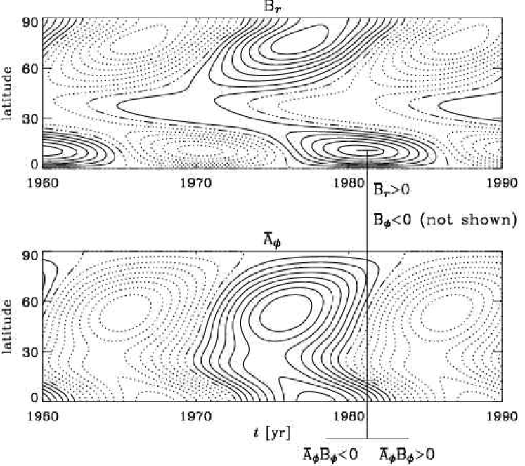
Figure 11.1: Mean dipole symmetry radial field, $\overline{B}_{r}$, reconstructed from the coefficients of Stenflo [32, 33] (upper panel). The corresponding toroidal component of the mean vector potential, $\overline{A}_{\phi}$, derived from $\overline{B}_{r}$ (lower panel). Solid contours denote positive values, dotted contours negative values. The solar cycle maximum of 1982 is highlighted, as is the latitude of 10^∘ where $\overline{B}_{r}$ was then strongest. The signs of various quantities at or around this epoch are also shown (see text for more details). Adapted from Ref. [411].

What is missing is a quantitative assessment of the relative magnitudes of large and small scale magnetic helicities. To get an idea about the sign and possibly the magnitude of the relative magnetic helicity of the longitudinally averaged field (denoted here by overbars), one should ideally calculate $2\int\overline{A}_{\phi}\overline{B}_{\phi}\,\mathrm{d}V$, which is the gauge-invariant magnetic helicity of Berger and Field for axisymmetric fields in a sphere (see Section 9.5). As a first step in that direction, one can determine $\overline{A}_{\phi}$ at the solar surface from the observed radial component of the magnetic field, $\overline{B}_{r}$, using

$$\overline{B}_{r}={1\over r\sin\theta}\,{\partial\over\partial\theta}\,\left(\sin\theta\overline{A}_{\phi}\right),\quad r=R_{\odot}.$$ (11.1)

This equation can easily be solved for $\overline{A}_{\phi}$ using the modal decomposition in spherical harmonics [411]; the result is shown in Fig. 11.1. Empirically, we know that $\overline{B}_{r}$ is approximately in antiphase with $\overline{B}_{\phi}$. Comparison of the two panels of Fig. 11.1 suggests that $\overline{A}_{\phi}\overline{B}_{\phi}$ was negative just before solar maximum ($t<1982\,{\rm yr}$) and positive just after ($t>1982\,{\rm yr}$). Thus, the present attempt to assess the sign of the magnetic helicity of the large scale field does not support nor exclude the possibility that the large scale field has positive magnetic helicity, as suggested by the tilt of bipolar regions.

11.2.3 Migration of activity belts and butterfly diagram

There are still a number of other rather long standing problems. Most important perhaps is the sense of migration of the magnetic activity belts on either side of the equator. This migration is traditionally believed to be associated with the phase velocity of the dynamo wave; see Section 6.5.2. However, this would be in contradiction with $\alpha>0$ (as expected in the northern hemisphere) and $\partial\Omega/\partial r>0$ (known from helioseismology [423]).

One of the currently favored models is the flux transport model where meridional circulation is assumed to be oriented such that, at the bottom of the convection zone, meridional circulation would advect the dynamo wave equatorward [424, 425, 426, 427, 355, 356, 428]. This proposal came originally quite as a surprise, because meridional circulation was normally always found to make dynamos nonoscillatory well before the anticipated advection effect could take place [301, 344, 348].

Whether or not the flux transport proposal is viable cannot be decided at present, because this model (and essentially all other solar dynamo models available so far) lack consistency with respect to the conservation of total (small and large scale) magnetic helicity. In addition, there are several other problems. With realistic profiles of differential rotation it is difficult to produce satisfactory butterfly diagrams [355]. It is also difficult to produce fields of dipolar rather ran quadrupolar parity [356], although this remains debatable [429].

Quite a different possibility is to invoke the near-surface shear layer in the outer 35 megameters of the sun [430, 431]. Here the angular velocity gradient is negative, giving rise to equatorward migration. For this scenario to work, one has to rely on turbulent downward pumping to prevent the magnetic field from buoyantly escaping through the surface. However, simulations of stratified convection have clearly demonstrated the dominance of pumping over magnetic buoyancy [203, 253, 331, 332, 333]; see also Section 6.4. There is obviously a lot more to be discussed in connection with this scenario, but the situation is still premature and it would go beyond the scope of this review. We refer instead to a recent paper [55] devoted specifically to this discussion.

11.2.4 The phase relation between poloidal and toroidal fields

Even if the problem of the migration direction of the toroidal activity belts was solved (for example by meridional circulation; see Section 11.2.3), there remains the problem of the phase relation between poloidal and toroidal field, provided the field was mainly generated at the bottom of the convection zone. Observations suggest that $B_{r}$ and $B_{\phi}$ are in antiphase. For example, when $B_{\phi}<0$ (as seen from the orientation of bipolar regions; see Fig. 6.1 for Cycle 21 during the year 1982) we have $B_{r}>0$ (as seen from synoptic magnetograms, see Fig. 11.1 at $t=1982\,{\rm yr}$), and vice versa [342, 343]. The basic problem is actually connected with the sense of the radial differential rotation, i.e. the fact that $\partial\Omega/\partial r>0$ in low solar latitudes. This always turns a positive $B_{r}$ into a positive $B_{\phi}$, and vice versa, regardless of the sign of the $\alpha$ effect. No convincing solution to this problem has yet been offered, although it has been suggested [432] that the problem might disappear in more realistic settings. Of course, in the near-surface shear layer, $\partial\Omega/\partial r$, so the problem with the phase relation would be solved in this scenario where the solar dynamo works in or is shaped by the near-surface shear layer [55].

11.2.5 The flux storage problem

Since the early eighties it was realized that flux tubes with a strength similar to or in excess of that in sunspots would float up to the surface in a time short ($\sim 50\,\mbox{days}$) compared with the dynamo time scale ($\sim 10\,{\rm yr}$). Therefore, magnetic buoyancy might act as an efficient sink term of mean toroidal field. This led to the suggestion [433] that the dynamo may operate in the lower part of the convection zone or just below it where magnetic flux tubes could stay in equilibrium. Model calculations [434, 435] have shown however that dynamos in thin layers tend to produce too many toroidal flux belts in each hemisphere [436], and that for an overshoot layer dynamo the layer must therefore not be less than about $30\,{\rm Mm}$ deep [354], which is much more than the helioseismologically implied thickness of the solar overshoot layer.

As mentioned above, it is also possible that the dynamo might still work in the convection zone proper, but that turbulent pumping brings the field continuously to the bottom of the convection zone [330, 331, 332, 354], from where strong toroidal flux belts can rise to the surface and form bipolar regions (Fig. 6.1). The end result might be similar in the sense that in both cases bipolar regions would be caused by flux tubes anchored mostly in the overshoot layer. It should also be emphasized that magnetic buoyancy might not only act as a sink in a destructive sense, but it can also contribute to driving an $\alpha$ effect [437, 438, 439, 440]. A conclusive picture cannot be drawn until we have a better understanding about things like magnetic and current helicity fluxes that now appear quite vital for allowing the solar dynamo to work on the observed 22 year time scale. Finally, one should bear in mind that it is also possible that the solar field in sunspots and in active regions does not even come from very deep, and that it originates primarily from the near-surface shear layer. In that case the actual sunspot formation might be the result of convective collapse of magnetic fibrils [441, 442], possibly facilitated by negative turbulent magnetic pressure effects [319] or by an instability [443] causing the vertical flux to concentrate into a tube.

11.2.6 Significance of the tachocline and differential rotation

The tachocline is the layer where the latitudinal differential rotation turns into rigid rotation [444]. This layer is now known to be quite sharp and to coincide with the bottom of the convection zone [430]. The reason the latitudinal differential rotation does not propagate with time deeper into the radiative interior is probably connected with the presence of a weak primordial magnetic field [445, 446, 447].

The tachocline is likely to be the place where the vertical shear gradient plays an important role in amplifying the toroidal magnetic field. This is perhaps not so much because the shear gradient is strongest at and just below the tachocline, but because the turbulent magnetic diffusivity is decreased, and because the magnetic field is pumped into this layer from above.

In the convection zone proper the differential rotation is in rough approximation spoke-like, i.e. nearly independent of spherical radius. Simulations, on the other hand, shear a strong tendency to produce angular velocity contours that are constant on cylinders [448]. This is generally associated with the Taylor-Proudman theorem, and is a well recognized difficulty in understanding the solar differential rotation [449, 450, 451]. It is also fairly well understood that solar-like departures from cylindrical contours could be achieved by the baroclinic term [452], $\bm{\nabla}s\times\bm{\nabla}T$, where $s$ and $T$ are specific entropy and temperature, respectively. In the convection zone, where the radial entropy gradient is small, a finite baroclinic term is mostly due to the latitudinal entropy gradient, so that

$$\varpi{\partial\Omega^{2}\over\partial z}\approx\hat{\bm{\phi}}\cdot(\bm{\nabla}s\times\bm{\nabla}T)\approx-{1\over r}{\partial s\over\partial\theta}{\partial T\over\partial r}<0,$$ (11.2)

where $\varpi=r\sin\theta$ is the cylindrical radius, $z=r\cos\theta$ is the distance from the equatorial plane, and $\hat{\bm{\phi}}$ is the unit vector in the azimuthal direction. Negative values of $\partial\Omega^{2}/\partial z$, in turn, require that the pole is slightly warmer than the equator (so weak that it cannot at present be observed. Achieving this in a simulation may require particular care in the treatment of the outer boundary conditions.

In order to understand the computational difficulties in dealing with the overshoot layer, we note that in and below the tachocline the total relaxation time is governed more strongly by the thermal time scale. Thus, if the system is slightly thrown out of balance, it will take a thermal time scale to reestablish a new equilibrium. Furthermore, as long as a new equilibrium state has not yet been reached, fairly strong amplitudes may develop, making the effective relaxation time even longer. While this will not be a problem for the sun, it may be a problem for simulations. In practice, this means that one has to be more careful setting up initial conditions and, perhaps most importantly, one should deliberately chose parameters whereby the thermal and acoustic time scales are not more disparate than what can be handled in a simulation. Nevertheless, keeping at least some representation of the tachocline, rather than neglecting it altogether, may be crucial. Without any representation of a tachocline it may not be possible to argue conclusively in favor of either the tachocline scenario or the near-surface shear layer scenario.

11.2.7 Luminosity variations

Cyclic variations of the magnetic field produce cyclic variations of the luminosity through variations of the superadiabatic gradient [433]. Although this basic picture has been confirmed in mean field dynamo models, the relative variations obtained are only $\delta L/L\sim 10^{-6}$ [451]. Larger values of a few times $10^{-3}$ can be obtained by making the upper boundary “partially reflecting”; see a recent paper by Pipin [453]. This emphasizes again that a realistic representation of the top boundary condition can be very important. This model also predicts variations of the hydrostatic balance and hence of the star’s quadrupole moment. This is important for stellar dynamos that are members of a binary system, because such variations can provide a means of determining the stars’ cycle period by measuring variations of the orbital period [454]. In Section 11.3 we discuss stellar dynamos in more detail.

11.2.8 Status of different solar dynamo model scenarios

Before turning attention to stellar dynamos we briefly summarize four different dynamo scenarios that are currently being discussed in the context of the sun. None of the models appear to be completely satisfactory, but the topic is advancing rapidly, as indicated at the end of this section.

• Distributed dynamo. An $\alpha$ effect is present throughout the entire convection zone, as described by Eq. (6.11) and calculated using a solar mixing length model [306]. At the bottom of the convection zone the sign of $\alpha$ reverses because of the sharp positive gradient of the turbulent rms velocity. Solutions have been calculated taking also into account Rädler’s $\bm{\Omega}\times\overline{\mbox{\boldmath$J$}}$ effect and other expressions. The model produces realistic butterfly diagrams including a solar branch [455]. Unfortunately, the published models use angular velocity profiles that are no longer compatible with modern helioseismological inversions.

• Overshoot dynamo. Here, $\alpha$ is only present in the overshoot layer, and it is artificially suppressed at high latitudes. Its sign in the northern hemisphere is negative because of the sharp positive gradient of the turbulent rms velocity. The resulting butterfly diagram looks reasonably acceptable, but for the model to be successful, the thickness of the overshoot layer cannot be less than $30\,{\rm Mm}$ [354], while helioseismology is now favoring values as small as $7\,{\rm Mm}$ [456].

• Interface dynamo. The sudden drop of the turbulent magnetic diffusivity below the overshoot layer is important. In the northern hemisphere $\alpha$ must be assumed to be negative and finite above the convection zone. The original model by Parker [457] worked with only radial differential rotation. When latitudinal differential rotation is included, only nonoscillatory solutions are found [458].

• Flux transport dynamo. Meridional circulation leads to equatorward migration of magnetic activity during the course of the cycle. The sign of $\alpha$ is positive in the northern hemisphere, and $\alpha$ is concentrated toward the upper layers of the convection zones. The magnetic diffusivity in the bulk of the convection zone is small. The resulting butterfly diagram is quite realistic [426], although the the parity issue remains to be clarified [356, 429].

The most popular model is currently the flux transport dynamo scenario [355, 356, 428]. However, there are a number of reasons why it might still be worthwhile pursuing the distributed dynamo scenario. Most important is the fact that magnetic tracers have an angular velocity that is close to the maximum angular velocity in the sun which is, according to helioseismology, only $35\,{\rm Mm}$ beneath the surface [430, 431]. This suggests that magnetic tracers such as sunspots might not be anchored very deeply. There are a number of other issues that may be more easily resolved within the framework of a distributed dynamo: instead of requiring a field strength of $100\,{\rm kG}$ (typical of all dynamos where the toroidal field emerges from the overshoot layer), only about $300\,{\rm G}$ may be required if the field is generated locally within the convection zone. Also, in the upper $35\,{\rm Mm}$ beneath the surface, the radial angular velocity gradient is negative, suggesting that a locally produced dynamo wave would migrate equatorward without invoking meridional circulation. These and a number of other arguments have been collected and discussed in Ref. [55]. Finally, it should be recalled that dynamos in fully convective spheres without any overshoot layer also produce magnetic activity. This will be discussed in more detail in the next section.

11.3 Stellar dynamos

Looking at stars other than the sun allows us to test the dependence of the dynamo on radius, on the thickness of the convection zone and, in particular, on the angular velocity of the star. In this section we summarize a few such dependencies and discuss whether they can be reproduced by dynamo models.

11.3.1 Fully convective stars

Toward the less massive stars along the main sequence the thickness of the convection zone increases relative to the stellar radius (although in absolute units the thickness remains around $200\,{\rm Mm}$) until the star becomes fully convective. Such stars would lack a lower overshoot layer which was often thought to be an important prerequisite of solar-like dynamos. On the other hand, turbulent pumping would in any case tend to concentrate the field toward the center of the star, and since the gravitational acceleration vanishes at the center, the magnetic field can probably still be stored for some time (if that was an issue).

Figure 11.2 shows a visualization of magnetic field lines of a self-consistent turbulence simulation of a fully convective spherical dynamo. In this simulation the dynamo is weakly supercritical. Following similar approaches by other groups [459, 460, 461, 462, 463], the star is embedded in a sphere, which avoids computational difficulties associated with coordinate singularities in explicit finite difference methods using spherical coordinates. The star’s radius is 27% of the solar radius and the mass is 21% of the mass of the sun.

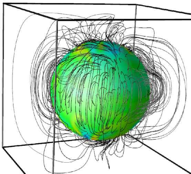
Figure 11.2: Magnetic field lines outside a model of a fully convective M-dwarf. Color coded is the radial field component on the surface of the star. Courtesy of W. Dobler [463].

Another class of fully convective stars are the T Tauri stars, i.e. stars that have not yet settled on the main sequence. These stars are generally known to spin very rapidly, so magnetic braking via magnetic field lines anchored in the surrounding protoplanetary accretion disc is usually invoked to explain the much slower rotation rate of evolved stars such as the sun [166]. It is also possible that young stars are mainly braked by a stellar wind if the star–disc becomes inefficient [464, 465].

11.3.2 Models of stellar cycles

Stars exhibiting cyclic behavior can cover a broad parameter range that allows us to test whether the dependence of cycle properties on stellar parameters agrees with what is expected from dynamo models. For orientation one can consider the marginally excited solution from linear theory and it is indeed common to look at plane wave solutions [466, 467, 468].

Several results have emerged from this type of analysis. Comparing models with different model nonlinearities ($\alpha$ quenching, feedback on the differential rotation, and magnetic buoyancy) it turns out [469] that only models with magnetic buoyancy as the dominant nonlinearity are able to produce a positive exponent $\sigma$ in the relation $\omega_{\rm cyc}/\Omega=c_{1}\mbox{Ro}^{-\sigma}$; see Eq. (2.1). We emphasize that it is not sufficient that $\omega_{\rm cyc}$ increases with $\Omega$. For example, an increase proportional to $\Omega^{0.5}$, which is found for classical dynamo models [62], is insufficient.

Meanwhile, there has been some uncertainty regarding the correct cycle frequency dependence on $\mbox{Ro}^{-1}$. We recall that in Fig. 2.8 there are two separate branches, both of which have a positive slope $\sigma$. On the other hand, a negative slope has been found when plotting $\omega_{\rm cyc}/\Omega$ versus the dimensional form of $\Omega$ (rather than the nondimensional $\mbox{Ro}^{-1}=2\Omega\tau_{\rm turnover}$) [470]. One may argue that the nondimensional form is to be preferred, because it is more general and it also yields a smaller scatter [61].

While ordinarily quenched dynamos tend to produce negative exponents $\sigma$ [62], ‘anti-quenched’ dynamos can produce the observed exponents when the dynamo alpha and the turbulent dissipation rate, $\tau^{-1}=\eta_{\rm t}k_{z}^{2}$, increase with field strength, e.g. like

$$\alpha=\alpha_{0}|B/B_{\rm eq}|^{n},\quad\tau^{-1}=\tau_{0}^{-1}|B/B_{\rm eq}|^{m},\quad m,n>0.$$ (11.3)

The motivation behind anti-quenching lies in the realization that the motions driving turbulent transport coefficients can be caused by magnetic instabilities. Examples of such magnetic instabilities include the magnetic buoyancy instability [438, 439, 440], the magneto-rotational instability [70, 201], and global instabilities of the tachocline differential rotation [356, 471].

Assuming that the dynamo operates in its fundamental mode (even in the nonlinear regime) one can apply the relations (6.39) and (6.40) for a fixed value $k_{z}$, where $k_{z}L=1$, where $L$ is the system size. This leads to two algebraic relations [59]

$$\tau_{0}^{-1}|B/B_{\rm eq}|^{m}=|{\textstyle{1\over 2}}\alpha_{0}\Omega^{\prime}|^{1/2}\,|B/B_{\rm eq}|^{n/2},$$ (11.4)

$$\omega_{\rm cyc}=\tau_{0}^{-1}|B/B_{\rm eq}|^{m}.$$ (11.5)

Dividing both equations by $\Omega$ and making use of the relation $\langle R_{\rm HK}^{\prime}\rangle\propto|B/B_{\rm eq}|^{\kappa}$ (usually $\kappa\approx 0.5$; see Section 2.2), we have

$$2\mbox{Ro}\,\langle R_{\rm HK}^{\prime}\rangle^{m/\kappa}=\left|{\alpha_{0}\Omega^{\prime}\over 2\Omega^{2}}\right|^{1/2}\langle R_{\rm HK}^{\prime}\rangle^{n/2\kappa},$$ (11.6)

$$\left|{\omega_{\rm cyc}\over\Omega}\right|=2\mbox{Ro}\,\langle R_{\rm HK}^{\prime}\rangle^{m/\kappa}.$$ (11.7)

For slow rotation $\alpha$ is proportional to $\Omega$, while for rapid rotation it is independent of $\Omega$ [310]. Likewise, for $\Omega^{\prime}$ the possibilities range from being independent of $\Omega$ [472] to being proportional to $\Omega^{0.7}$ [473]. To account for these different possibilities, we make the more general assumption

$$\left|{\alpha_{0}\Omega^{\prime}\over\Omega^{2}}\right|\sim\mbox{Ro}^{-q},$$ (11.8)

where $q$ can be anywhere between $-0.3$ and $-2$, depending on the assumed $\alpha(\Omega)$ and $\Omega^{\prime}(\Omega)$ dependencies. We thus have

$$\mbox{Ro}\,\langle R_{\rm HK}^{\prime}\rangle^{m/\kappa}\sim\mbox{Ro}^{-q/2}\langle R_{\rm HK}^{\prime}\rangle^{n/2\kappa},$$ (11.9)

$$\left|{\omega_{\rm cyc}\over\Omega}\right|\sim\mbox{Ro}\,\langle R_{\rm HK}^{\prime}\rangle^{m/\kappa}.$$ (11.10)

Using the definitions (2.1), i.e. $\langle R^{\prime}_{\rm HK}\rangle\sim\mbox{Ro}^{-\mu}$ and $|\omega_{\rm cyc}/\Omega|\sim\mbox{Ro}^{-\sigma}$, together with $\sigma=\mu\nu$ (see Section 2.2), we have

$$\mbox{Ro}^{1-m\mu/\kappa}\sim\mbox{Ro}^{-q/2-n\mu/2\kappa},$$ (11.11)

$$\mbox{Ro}^{-\mu\nu}\sim\mbox{Ro}^{1-m\mu/\kappa},$$ (11.12)

so $\mu\nu=m\mu/\kappa-1=q/2+n\mu/2\kappa$, which yields explicit results for the dynamo exponents $m$ and $n$,

$$m=\kappa(\nu+1/\mu),$$ (11.13)

$$n=\kappa(2\nu-q/\mu).$$ (11.14)

Note that $m$ is independent of the rather uncertain value of $q$. In Table LABEL:TBST98 we summarize the results obtained from the subset of stars that show cycles [57]. The different branches, which are separated by a factor of about 6, might be associated with the occurrence of different magnetic instabilities in different parameter regimes, but no definitive proposal can be made at this point. In this table we also give the results for an expanded sample [61] where, in addition to the chromospheric emission, photometric and other cycle data have been used.

Table 11.2: Summary of observable parameters characterizing stellar cycle properties ($\sigma$, $\nu$, and $\mu$) and the corresponding model parameters $m$ and $n$, introduced in Eq. (11.3); see Ref. [59]. We recall that the values of $\sigma$ and $\nu$ are obtained from separate fits and thus do not obey the relation $\sigma=\mu\nu$. Since the scatter in the plots giving $\sigma$ is larger than in those giving $\nu$, we discard the former in the calculation of $m$ and $n$. In the first two rows, only stars from the original Wilson sample [474] with grades good and excellent are considered [59]. This sample does not include superactive stars. In the last three rows, stars from the expanded sample [61] were considered. For most of them, no calcium data are available, and therefore only cycle periods are considered, so $\nu$ is not being determined.

Stars sample $\sigma$ $\nu$ $\mu$ $m$ $n$ inactive grade: (0.46) 0.85 0.99 0.9 0.9–1.7 active excellent+good (0.48) 0.72 0.99 0.8 0.8–1.6 inactive expanded $\approx 0.5$ 1 0.75 0.5–1.5 active sample $\approx 0.5$ 1 0.75 0.5–1.5 superactive Ref. [61] $-0.43$ 0.28 $-0.43$–0.57

Although it is well recognized that single mode approximations are not sufficient to solve the dynamo equations as stated [see, e.g., Eq. (9.14)], the one-mode equations may still turn out to be closer to physical reality, because there is now evidence from data of accretion disc simulations that the spectral sensitivity of the turbulent transport coefficients is highest at small wavenumbers [337]. In other words, the multiplication $\alpha\overline{\bm{B}}$ in Eq. (6.3) should be replaced by a convolution $\alpha\circ\overline{\bm{B}}$, where $\alpha$ would now be an integral kernel. In wavenumber space, this would correspond to a multiplication with a $k$-dependent $\hat{\alpha}$ such that $\hat{\alpha}(k)$ is largest for small values of $k$. One may hope that future simulations will shed more light on this possibility.

11.3.3 Rapidly rotating stars or planets

An important outcome of mean field calculations in the presence of rapid rotation (not captured by the analysis in Section 10) is the prediction that the $\alpha$ effect becomes highly anisotropic and takes asymptotically the form [221]

$$\alpha_{ij}=\alpha_{0}\left(\delta_{ij}-\Omega_{i}\Omega_{j}/\Omega^{2}\right),$$ (11.15)

which implies that, if the angular velocity points in the $\hat{\mbox{\boldmath$z$}}{}$ direction, for example, i.e. $\bm{\Omega}=\Omega\hat{\mbox{\boldmath$z$}}{}$, the vertical component of $\alpha$ vanishes, i.e. $\alpha_{zz}\to 0$ for $\mbox{Ro}^{-1}\equiv 2\Omega\tau\gg 1$. For calculations of axisymmetric and nonaxisymmetric models using large but finite values of $\mbox{Ro}^{-1}$ see Refs [354, 475].

In Eq. (11.15) we stated the asymptotic form of the $\alpha$ tensor in the limit of rapid rotation. Such a highly anisotropic $\alpha$ tensor is known to lead to strong nonaxisymmetric magnetic field configurations [220, 476]. Such an $\alpha$ effect has been applied to modeling the magnetic fields of the outer giant planets that are known to have very large values of $\mbox{Ro}^{-1}$. Simulations using parameters relevant to the outer giant planets of our solar system show that these bodies may have a magnetic field that corresponds to a dipole lying in the equatorial plane [475, 477].

The biggest enemy of nonaxisymmetric fields is always differential rotation, because the associated wind-up of the magnetic field brings oppositely oriented field lines close together, which in turn leads to enhanced turbulent decay [341]. This is quite different to the case of an axisymmetric field, where the wind-up brings equally oriented field lines together, which leads to magnetic field enhancements; i.e. the $\Omega$ effect.

As the value of $\mbox{Ro}^{-1}$ increases, the $\alpha$ tensor becomes not only highly anisotropic, but the magnitudes of all components decreases. This is a common phenomenon known as ‘rotational quenching’ that affects virtually all turbulent transport coefficients. An important turbulent transport coefficient that we will not say much about here is the so-called $\Lambda$ effect (modeling the toroidal Reynolds stress), is responsible for driving differential rotation in stars including the sun. Very rapidly rotating stars are therefore expected to have very little relative differential rotation, which is indeed observed [478]. This means that the $\alpha\Omega$ dynamo will stop working and one would therefore expect an anisotropic $\alpha^{2}$ dynamo mechanism to operate in rapidly rotating bodies with outer convection zones. This means that such stars should generate a predominantly nonaxisymmetric field. There are indeed numerous observational indications for this [479, 480]. It should be noted, however, that already the large scale flow that is generated by the magnetic field and the Reynolds stress (i.e. the $\Lambda$ effect) tend to make the field nonaxisymmetric [481]. In addition, in rapidly rotating stars all motions tend to be mostly in cylindrical surfaces (Taylor-Proudman theorem). This effect is believed to cause starspots to emerge mostly at high latitudes in rapidly rotating stars [482, 483]. Furthermore, the convective motions tend to be column-like [484]. This led to the proposal of the Karlsruhe dynamo experiment where the flow is similarly column-like.

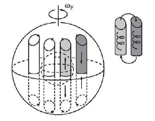
Figure 11.3: Convection columns in a rapidly rotating spherical shell. Courtesy of A. Yoshizawa [22].

11.3.4 Connection with the Karlsruhe dynamo experiment

In the Karlsruhe dynamo experiment, liquid sodium is pumped upward and downward in alternating channels [485]. Each of these channels consist of an inner and an outer pipe, and the walls of the outer one are arranged such that the flow follows a swirling pattern; see Fig. 11.4. The swirl in all columns is such that the associated kinetic helicity has the same sign everywhere. In fact, locally such a flow is strongly reminiscent of the Roberts flow (Section 4.2.2) that is known to generate a Beltrami field in the plane perpendicular to the direction of the pipes, i.e. $(\cos kz,\sin kz,0)$ if $z$ is the direction of the pipes and the phase shift in $z$ has been ignored; see Section 8.4. On a global scale such a field corresponds to a dipole lying in the $xy$ plane, and perpendicular to the $\bm{z}$ direction; see Fig. 11.4. Applied to the earth, it would therefore correspond to a nonaxisymmetric field and would not really describe the magnetic field of the earth, although it might be suitable for explaining the magnetic fields of the other giant planets Uranus and Neptune [475] that are indeed highly nonaxisymmetric [486].

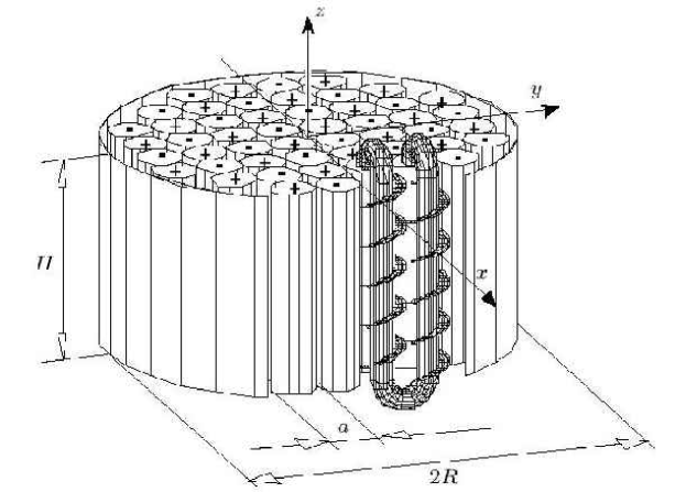
Figure 11.4: The dynamo module of the Karlsruhe dynamo experiment. The signs + and – indicate that the fluid moves in the positive or negative $z$–direction, respectively, in a given spin generator. Courtesy R. Stieglitz and U. Müller [485].

11.3.5 Chaos and intermittency

The search for more complicated temporal and spatio-temporal patterns has always been popular in mean field dynamo research. In spatially resolved models (as opposed to one-mode approximations [487]) it was for a long time difficult to find spatially well resolved solutions that showed chaotic or even just quasiperiodic behavior. In fact, it was thought to be essential to invoke an additional explicit time dependence of the form of dynamical quenching [10, 11, 12]. More recently it turned out that quasiperiodic and chaotic solutions to the mean field dynamo equations are possible when the dynamo number is raised sufficiently [346, 488]. Intermittent behavior has also been found when the feedback on the mean flow is taken into account [489, 490]. For moderately large dynamo numbers, such solutions require however small turbulent magnetic Prandtl numbers, which is an assumption that is not confirmed by simulations [395]. Nevertheless, intermittent solutions of this or some other kind are thought to be relevant in connection with understanding the intermittency of the solar cycle and the occurrence of grand minima [491, 492].

The question is of course how much one can trust such detailed predictions of mean field theory when we are still struggling to confirm the validity of mean field theory in much simpler systems. One may hope that in the not too distant future it will be possible to compare mean field models with simulations in somewhat more extreme parameter regimes where quasi-periodic and chaotic behaviors are expected to occur.

11.3.6 Dynamos in proto-neutron stars

The $\sim 10^{13}\,{\rm G}$ magnetic field of neutron stars is traditionally thought to be the result of compressing the magnetic field of its progenitor star. The difficulty with this explanation is that in the early phase of a neutron star (proto-neutron star) the neutrino luminosity was so immense and the neutrino opacity high enough that the young neutron star must have been convectively unstable. Although this phase lasts for only $\sim 20$ seconds, this still corresponds to some $10^{4}$ turnover times, because gravity is so strong that the turnover time is only of the order of milliseconds. This would be long enough to destroy the primordial magnetic field and to regenerate it again by dynamo action [493, 494].

If the field was initially generated by an $\alpha$ effect, and if the associated small scale magnetic helicity has been able to dissipate or escape through the outer boundaries, the field must have attained some degree of magnetic helicity. Once the turbulence has died out, such a helical field decays much more slowly than nonhelical fields [495], and it would have attained the maximum possible scale available in a sphere. Such a field may well be that of an aligned or inclined dipole, as observed. There are also some interesting parallels between dynamo action in decaying turbulence in neutron stars and that in the planned time-dependent dynamo experiment in Perm based on decaying turbulence in liquid sodium [496]. In the Perm experiment, a rapidly spinning torus with liquid sodium will suddenly be braked, which leads to swirling turbulence due to suitable diverters on the wall of the torus.

11.4 Accretion disc dynamos

When dynamo theory was applied to accretion discs, it seemed at first just like one more example in the larger family of astrophysical bodies that host dynamos [497, 498, 499, 500]. Later, with the discovery of the magneto-rotational instability [69, 70], it became clear that magnetic fields are crucial for maintaining turbulence in accretion discs [501, 502], and that this can constitute a self-excited process whereby the magnetic field necessary for the magneto-rotational instability is regenerated by dynamo action.

Simulations in a local (pseudo-periodic shearing box) geometry have shown that this self-excited system can act both as a small scale dynamo if there is no vertical density stratification [265, 413] and as a large scale dynamo if there is stratification [201, 503].

From a turbulence point of view it is interesting to note that the flow is highly anisotropic with respect to the toroidal direction. This is true even down to the smallest scale in the simulations. From a mean field dynamo point of view this system (with stratification included) is interesting because it is an example of a simulation of a dynamo where the turbulence occurs naturally and is not driven by an artificial body force. This simulation is also an example where an $\alpha$ effect could be determined [504].

11.4.1 Dynamo waves in shearing sheet simulations

When the vertical field boundary condition is used, i.e. $B_{x}=B_{y}=0$ on $z=z_{\rm top}$ and $z_{\rm bot}$, the horizontal flux through the box is no longer conserved, and hence the horizontal components of the horizontally averaged field may be different from zero, i.e. $\overline{B}_{x}\neq 0\neq\overline{B}_{y}$, even though they may be zero initially. This is exactly what happened in the shearing box dynamo simulation when these boundary conditions where used. In Fig. 11.5 we show the space-time diagram (or butterfly diagram in solar physics) of the mean magnetic field of such a simulation [337, 504]. In this particular simulation the symmetry of the magnetic field has been restricted to even parity about $z=0$, so the computation has been carried out in the upper disc plane, $0<z<L_{z}$, where $L_{z}=2H$ is the vertical extent of the box, $H$ is the gaussian scale height of the hydrostatic equilibrium density, and $z=0$ corresponds to the equatorial plane.

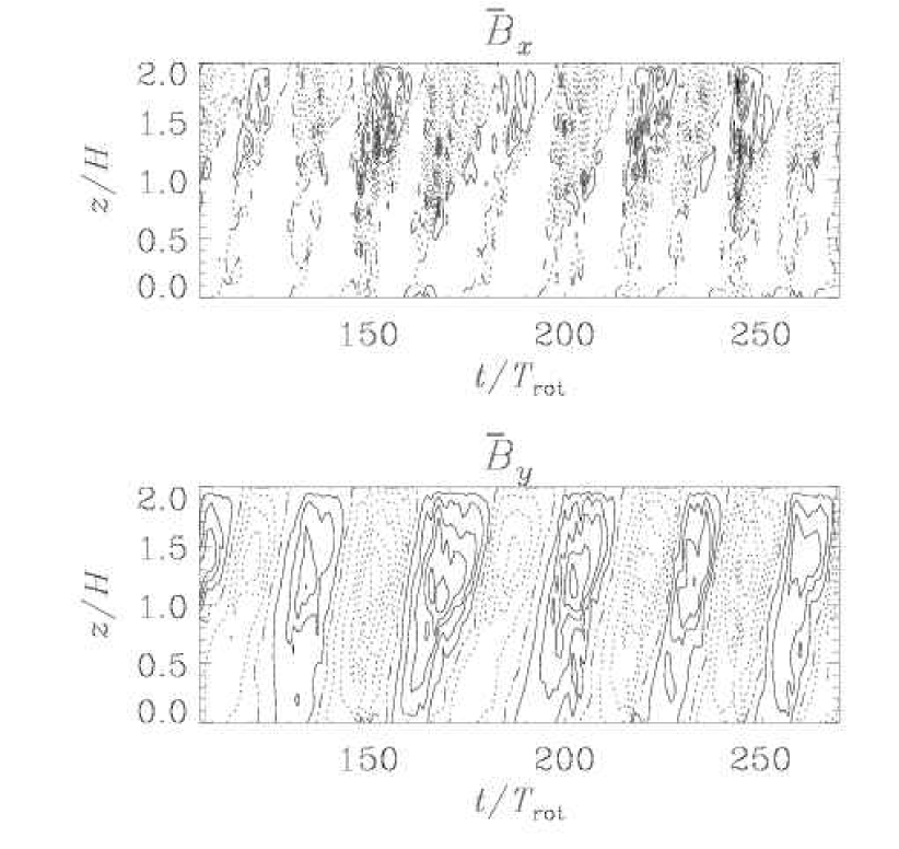
Figure 11.5: Horizontally averaged radial and toroidal magnetic fields, $\overline{B}_{x}$ and $\overline{B}_{y}$ respectively, as a function of time and height, as obtained from the fully three-dimensional simulation of a local model of accretion disc turbulence. Time is given in units of rotational periods, $T_{\rm rot}$. (No smoothing in $z$ or $t$ is applied.) Dotted contours denote negative values. Adapted from Ref. [337].

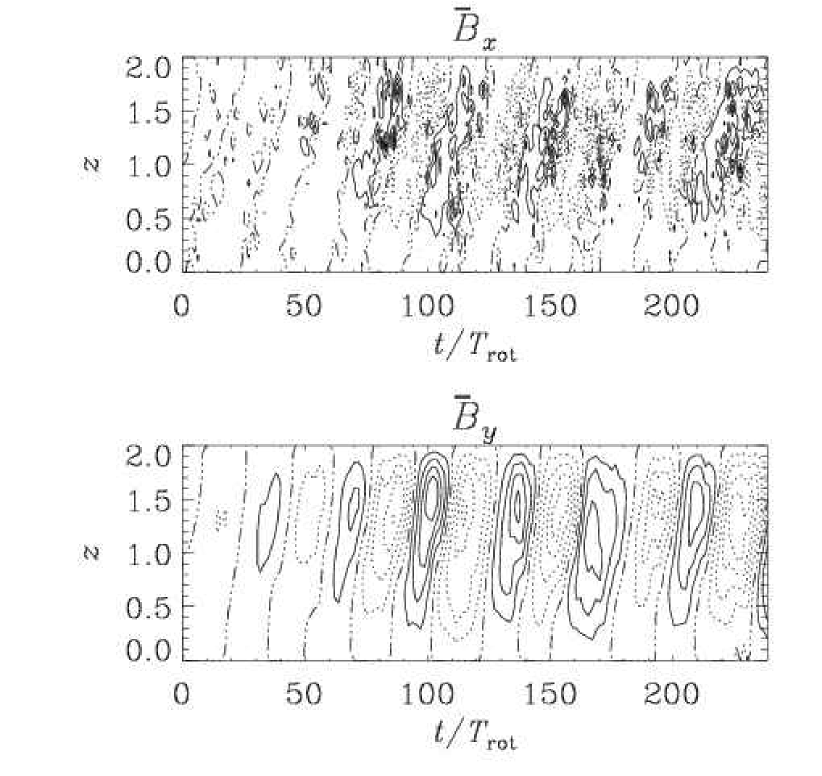
Figure 11.6: Resulting $\overline{B}_{x}$ and $\overline{B}_{y}$ from a mean field calculation with negative $\alpha$ effect ($\alpha_{0}=-0.001\Omega H$), together with a 10 times stronger noisy components ($\alpha_{N}=0.01\Omega H$), and a turbulent magnetic diffusivity ($\eta_{0}=0.005\Omega H^{2}$), producing a cycle period of about 30 orbits. Adapted from Ref. [337].

It is interesting to note that the spatio-temporal behavior obtained from the three-dimensional simulations resembles in many ways what has been obtained using mean field models; see Section 6.5.2. Note, however, that in Fig. 11.5 dynamo waves propagate in the positive $z$ direction, i.e. $c>0$ in Eq. (6.42). This requires $\alpha<0$, which is indeed consistent with the sign of $\alpha$ obtained earlier by means of correlating ${\cal E}_{y}$ with $\overline{B}_{y}$ [201, 504], but it is opposite to what is expected in the northern hemisphere (upper disc plane) from cyclonic events.

Mean-field model calculations confirm that the space-time diagram obtained from the simulations (Fig. 11.5) can be produced with a negative $\alpha$ effect of the magnitude found by correlating ${\cal E}_{y}$ with $\overline{B}_{y}$ and a turbulent magnetic diffusivity comparable to the turbulent kinematic viscosity obtained by measuring the total (Reynolds and Maxwell) stress [201]. The directly determined $\alpha$ effect is however so noisy, that it is hard to imagine that it can produce a mean field that is as systematic as that in the simulation (Fig. 11.5). However, model calculations show also that, even when the noise level of $\alpha$ exceeds the average value by a factor of 10, the resulting mean field is still sufficiently coherent (Fig. 11.6) and in fact similar to the field obtained from the simulations [337].

A negative sign of the $\alpha$ effect in accretion discs may arise because of two important circumstances. First, the vertical velocity fluctuation is governed by magnetic buoyancy and second, shear is important. Following a simple argument of Ref. [360], the $\alpha$ effect is dominated by the contribution from the momentum equation and the toroidal magnetic field, $B_{y}$,

$${\partial{\cal E}_{y}\over\partial t}\sim\overline{\dot{u}_{z}b_{x}}\sim\left({\overline{b_{y}b_{x}}\over p_{0}}g\right)\overline{B}_{y}\equiv\tilde{\alpha}_{yy}\overline{B}_{y},$$ (11.16)

where the vertical acceleration is assumed to be mostly due to magnetic buoyancy, i.e. $\dot{u}_{z}\approx-(\delta\rho/\rho_{0})\,g$ and $-\delta\rho/\rho_{0}=\delta\bm{B}^{2}/(2p_{0})\approx\overline{B}_{y}b_{y}/p_{0}$, where we have linearized with respect to the fluctuations. In accretion discs the shear is negative, i.e. $\partial\overline{U}_{y}/\partial x<0$, and therefore $\overline{b_{y}b_{x}}<0$. If this effect does indeed dominate, the $\alpha$ effect will be negative, i.e. $\alpha_{yy}=\tau\tilde{\alpha}_{yy}<0$. Subsequent work based on FOSA confirms the possibility of a negative value of $\alpha_{yy}$ for sufficiently strong shear [505], as is indeed present in accretion discs. However, because of the competing effect to drive a positive $\alpha$ effect from thermal buoyancy, the sign of $\alpha_{yy}$ changes to the conventional sign for weak shear.

In summary, local disc simulations suggest the possibility of a doubly-positive feedback from both the magneto-rotational instability and the dynamo instability, giving rise to small scale magnetic fields (if there is no stratification) and large scale fields (if there is vertical stratification). The magnetic energy exceeds the kinetic energy, but is below the thermal energy; see Section 4.1. The latter gives information about the dimensionless value of the Shakura-Sunyaev viscosity parameter which is typically around 0.01 [201, 265, 413]. Large scale field generation is compatible with that from a negative $\alpha$ which, in turn, produces oscillatory mean fields that are symmetric about the mid-plane. This is consistent with mean field theory, which also predicts that, with the same vertical field boundary conditions, the field should be oscillatory and symmetric about the midplane, i.e. quadrupole-like.

When the boundary conditions in the accretion disc simulations are changed to perfectly conducting boundaries, the situation changes entirely; the field becomes non-oscillatory and antisymmetric about the midplane, i.e. dipole-like [360]. However, this drastic change is quite compatible with mean-field theory which also predicts that with perfectly conducting boundaries a negative $\alpha$ in the upper disc plane should give rise to a non-oscillatory field that is antisymmetric about the midplane. Having thus established this type of correspondence between simulations and mean field theory, one is tempted to apply mean field theory with a negative $\alpha$ in the upper disc plane to a global geometry. It turns out that with a conducting halo, the most easily excited solution is also antisymmetric about the midplane (i.e. dipolar) and non-oscillatory. Such models have been discussed in connection with outflows from dynamo active accretion discs, as will be discussed further in the next section.

11.4.2 Outflows from dynamo active discs

It is now commonly believed that all accretion discs have undergone a phase with strong outflows. One mechanism for driving such outflows is magneto-centrifugal acceleration [506]. The magnetic field necessary might be the field that is dragged in from the embedding environment when the disc forms, but it might also be dynamo generated [507]. In Fig. 11.7 we present a numerical solution of such a model [508], where the dynamo is a mean field $\alpha\Omega$ dynamo with negative $\alpha$ effect [201]. In the presence of open boundaries considered here, the most easily excited solution has dipolar symmetry about the equatorial plane [509].

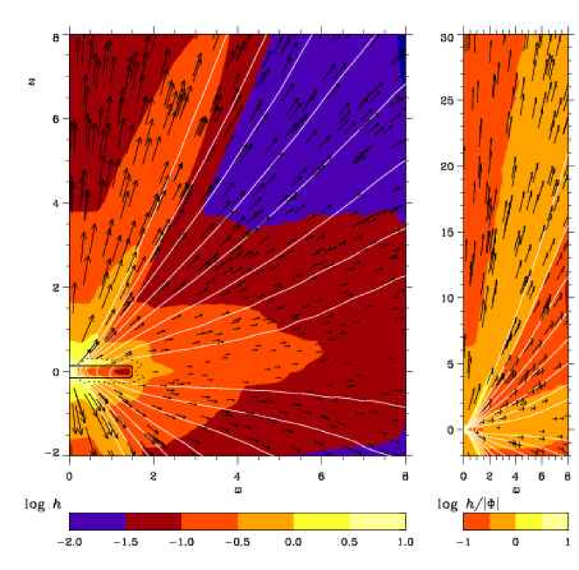
Figure 11.7: Outflow from a dynamo active accretion disc driven by a combination of pressure driving and magneto-centrifugal acceleration. The disc represents a protostellar disc, whose tenuous outer regions will are heated by the magnetic field. This pressure contributes to hydrostatic support, which is changed only slightly by the finite outflow velocities. The extent of the domain is $[0,8]\times[-2,30]$ in nondimensional units (corresponding to about $[0,0.8]\,{\rm AU}\times[-0.2,3]\,{\rm AU}$ in dimensional units). Left panel: velocity vectors, poloidal magnetic field lines and gray scale representation of $h$ in the inner part of the domain. Right panel: velocity vectors, poloidal magnetic field lines and normalized specific enthalpy $h/|\Phi|$ in the full domain. Adapted from Ref. [508].

Three-dimensional simulations of dynamo action in accretion disc tori have confirmed that the magneto-rotational instability can sustain a magnetic field also in such a global model [510, 511, 512, 513]. These simulations are now also beginning to show the formation of outflows that are clearly associated with large scale fields generated in the disc. The presence of large scale fields, and in particular its vertical component, is responsible for increased values of the dimensionless value of the Shakura-Sunyaev viscosity parameter which is now typically 0.1 [513].

11.5 Galactic dynamos

We saw in Section 2.4 that spiral galaxies have large scale magnetic fields of the order of a few $10^{-6}\,{\rm G}$, coherent on scales of several kpc, and also highly correlated (or anti-correlated) with the optical spiral arms. Does the mean field turbulent dynamo provide a viable model for understanding the origin such fields? We discuss below a number of observed properties of galactic fields which favor a dynamo origin of disc galaxy magnetic fields. However the strength of the field itself may not be easy to explain, in view of the helicity constraint.

11.5.1 Preliminary considerations

To begin with, all the ingredients needed for large scale dynamo action are present in disc galaxies. There is shear due to differential rotation and so any radial component of the magnetic field will be efficiently wound up and amplified to produce a toroidal component. A typical rotation rate is $\Omega\sim 25\,{\rm km}\,{\rm s}^{-1}\,{\rm kpc}^{-1}$ (at $r\approx 10\,{\rm kpc}$), and for a flat rotation curve ($\overline{U}_{\phi}=\Omega R=\mbox{constant}$) the shear rate, defined as $S=R\Omega^{\prime}\equiv R\mathrm{d}\Omega/\mathrm{d}R$, would be the same, i.e. $S=-\Omega$. This corresponds to a rotation time of $\sim 2\pi/\Omega\sim 2.5\times 10^{8}\,{\rm yr}$. So, in a Hubble time ($\sim 10^{10}\,{\rm yr}$) there have been about $40-50$ rotations. If only shear were involved in the generation of the galactic field, a fairly strong primordial seed field of $\sim 10^{-7}$ G would be required just after the galaxy formed. (We will also discuss other problems with such a primordial hypothesis below.)

A mechanism to exponentiate the large scale field, like for example the $\alpha\Omega$ dynamo, is therefore desirable. An $\alpha$ effect could indeed be present in a disc galaxy. First, the interstellar medium in disc galaxies is turbulent, mainly due to the effect of supernovae randomly going off in different regions. In a rotating, stratified medium like a disc galaxy, such turbulence becomes helical (Section 10.3). Therefore, we potentially have an $\alpha$ effect and so we expect $\alpha\Omega$ mean field dynamo action. Typical parameters for this turbulence are, a velocity scale $v\sim 10\,{\rm km}\,{\rm s}^{-1}$, an outer scale $l\sim 100\,{\rm pc}$ giving an eddy turnover time $\tau\sim l/v\sim 10^{7}$ yr. This yields an estimate of the turbulent diffusion coefficient, $\eta_{\rm t}\sim{\textstyle{1\over 3}}vl\sim 0.3\,{\rm km}\,{\rm s}^{-1}\,{\rm kpc}$ or $\eta_{\rm t}\sim 10^{26}\,{\rm cm}^{2}\,{\rm s}^{-1}$. The inverse Rossby (or Coriolis) number is $\sim 2\Omega\tau\sim 0.6$ (see Table LABEL:TRossby, where we have taken $\Omega=30\,{\rm km}\,{\rm s}^{-1}\,{\rm kpc}^{-1}$) and so we can use Eq. (10.57) to estimate $\alpha$ due to rotation and stratification. This gives $\alpha\sim\tau^{2}\Omega(v^{2}/h)\sim 0.75\,{\rm km}\,{\rm s}^{-1}$, where $h\sim 400\,{\rm pc}$ is the vertical scale height of the disc. So the turbulence is only weakly helical; nevertheless the degree of helicity ($\sim 5-10\%$) is sufficient for inducing large scale dynamo action, because the $\Omega$ effect is strong enough to make the $\alpha\Omega$ dynamo supercritical.

We gave a brief discussion of the simplest form of the mean field dynamo equations appropriate for a thin galactic disc in Section 6.5.5, following Ref. [77]; here we just gather some important facts. We recall that two dimensionless control parameters,

$$C_{\Omega}=Sh^{2}/\eta_{\rm t},\quad C_{\alpha}=\alpha h/\eta_{\rm t},$$ (11.17)

measure the strengths of shear and $\alpha$ effects, respectively. (Note that these are identical to the $R_{\Omega}$ and $R_{\alpha}$ commonly used in galactic dynamo literature.) For the above galactic parameters, the typical values are $C_{\Omega}\approx-10$ and $C_{\alpha}\approx 1$, and so $|C_{\Omega}|\gg C_{\alpha}$. Dynamo generation is controlled by the dynamo number $D=C_{\Omega}C_{\alpha}$, whose initial ‘kinematic’ value we denote by $D_{0}$. Exponential growth of the field is possible in the kinematic stage, provided $|D_{0}|>D_{\rm crit}$, where the critical dynamo number $D_{\rm crit}\sim 6...10$, depending on the exact profile adopted for $\alpha(z)$. Modes of quadrupole symmetry in the meridional $(Rz)$ plane are the easiest to excite in the case of a thin disc with $D<0$. Further the growth rate in the kinematic regime given by (6.47) has a numerical value,

$$\gamma\approx{\eta_{\rm t}\over h^{2}}\left(\sqrt{|D|}-\sqrt{D_{\rm crit}}\right)\approx(1...10)\,{\rm Gyr}^{-1}$$ (11.18)

The dynamo is generally supercritical, and the value of $\gamma$ evaluated locally at different radial position is positive for a large range of radii, and so galactic fields can be indeed grow exponentially from small seed values. Furthermore, in a Hubble time scale of $10^{10}\,{\rm yr}$, one could exponentially grow the field by a factor of about ${\rm e}^{30}\approx 10^{13}$, provided the growth rate determined in the kinematic regime were applicable. In this case, even a small field of order $10^{-19}$ G would in general suffice as the initial seed magnetic field; with galaxies at higher redshift requiring a larger seed magnetic field. We shall discuss below how the nonlinear restrictions, due to helicity conservation, may alter this picture. Before this, we first gather some of the observational indications which favor a dynamo origin for the galactic field, nicely reviewed by Shukurov [515, 516].

11.5.2 Observational evidence for dynamo action

The magnetic pitch angle

The simplest piece of evidence for dynamo action is just the form of the magnetic field lines as projected onto the disc. It is seen that the regular magnetic field in spiral galaxies is in the form of a spiral with pitch angles in the range $p=-(10^{\circ}\ldots 30^{\circ})$, where a negative $p$ indicates a trailing spiral. Note that for dynamo action one needs to have non-zero $\overline{B}_{R}$ and $\overline{B}_{\phi}$, or a non-zero pitch angle for the magnetic field lines projected onto the disc. A purely azimuthal field, with $\overline{B}_{R}=0$, will decay due to turbulent diffusion, and the same is true for a purely radial field. A simple estimate of the pitch angle can be obtained from the ‘no-$z$’ approximation [357] to the dynamo equations, whereby one replaces $z$ derivatives by just a division by $h$. Substituting also $\overline{B}_{R},\overline{B}_{\phi}\propto\exp{\gamma t}$, this gives

$$\left(\gamma+{\eta_{\rm t}\over h^{2}}\right)\overline{B}_{R}=-{\alpha\overline{B}_{\phi}\over h},\quad\left(\gamma+{\eta_{\rm t}\over h^{2}}\right)\overline{B}_{\phi}=S\overline{B}_{R}.$$ (11.19)

One derives a rough estimate for the ratio [515]

$$\tan p={\overline{B}_{R}\over\overline{B}_{\phi}}\approx-\left({\alpha\over-Sh}\right)^{1/2}=-\left({C_{\alpha}\over|C_{\Omega}|}\right)^{1/2}\approx-{l\over h}\left({\Omega\over|S|}\right)^{1/2}.$$ (11.20)

For $l/h=1/4$ and a flat rotation curve with $\Omega=-S$, one then gets $p\sim-14^{\circ}$. This is in the middle of the range of observed pitch angles in spiral galaxies. More detailed treatments of galactic dynamos [77] confirm this simple estimate. The above estimate is based on kinematic theory, and comparison with observations should preferably done with models including nonlinear effects. However, similar pitch angles are also obtained when one considers some simple nonlinear dynamo models [517]; see also the case of models for M31 in Ref. [518]. (The no-$z$ approximation also gives an estimate for $\gamma$ as in Eq. (11.18) but with the crude estimate $D_{\rm crit}=1$.)

An alternative hypothesis to the dynamo is that galactic magnetic fields are simply strong primordial fields that are wound up by differential rotation (see Refs [519, 520] and references therein). In this case, detailed analysis [520] shows that differential rotation leads a field which rapidly reverses in radius (on scales $\sim 100\,{\rm pc}$). More importantly the field is also highly wound up with pitch angles of order $p<1^{\circ}$, clearly much smaller than the observed values. In Ref. [520], it is argued that streaming motions in spiral arms would nevertheless lead to a field-aligned along the spiral; but away from the arms the field will be nearly toroidal. Clearly, in the case of NGC6946 it is the field in between the arms which has a spiral form with moderately large pitch angles with an average $p\sim 35^{\circ}$ for several of the magnetic arms [96]. Also in the case of M31, although the field itself occupies a ring-like region, the field lines are still in the form of spirals with pitch angles $\sim 10^{\circ}\ldots 20^{\circ}$ [521].

Another possibility is that the primordial field is not tightly wound up because turbulent diffusion compensates for the winding due to shear [522]. In this case there would be a balance between shear and turbulent diffusion, and from the toroidal part of Eq. (11.19) one can estimate $\overline{B}_{R}/\overline{B}_{\phi}\sim 1/C_{\omega}$; which implies $p\sim 6^{\circ}$ for $C_{\Omega}\sim 10$. This is larger than the pitch angle determined neglecting turbulent diffusion, but may still not be large enough to account for the observed range of $p$ in galaxies. Also one would need a constant source of $\overline{B}_{R}$, which could perhaps be due to accretion, since otherwise turbulent diffusion (without an $\alpha$ effect) will cause $\overline{B}_{R}$ to decay. The galactic dynamo on the other hand provides a natural explanation for the observed pitch angles of the regular magnetic field.

Even vertical symmetry of the field in the Milky Way

Another argument in favor of the galactic dynamo theory is the observed symmetry properties of the regular magnetic field about the galactic equator. Dynamo theory predicts that the toroidal and radial field components should be symmetric about the equator. The even parity mode has a larger scale of variation in the vertical direction and is therefore subject to a weaker turbulent diffusion than the odd parity mode [77]. A wavelet analysis of the Faraday rotation measures of extragalactic sources indeed indicates that the horizontal components of the regular magnetic field have even parity, that is they are similarly directed on both sides of the disc [109].

Such an even parity field can be produced from a primordial field if it is originally almost parallel to the disc plane. However, such a field would still suffer the excessive winding mentioned above. On the other hand, it is equally likely that a primordial field has a large component parallel to the rotation axis (entering through $z<0$ and exiting through $z>0$). In this case one would have a dipole structure for the wound up primordial field, which is not supported by the analysis of [109]. (As mentioned earlier, the determination of the magnetic field structure from Faraday rotation can be complicated by local perturbations.) Further, as discussed in Section 2.4 there was some evidence from the discovery of linear non thermal filaments perpendicular to the galactic plane, of a dipolar field in the central few hundred parsecs of our galaxy, which could be explained on the basis of a primordial field [523]. However the latest surveys for such linear filaments [113], no longer strongly support such a simple picture, and the observational situation needs to be clarified.

The azimuthal structure of disc galaxy fields

The kinematic growth rates predicted by an axisymmetric galactic dynamo are also the largest for purely axisymmetric field structures. Of course the spiral structure induces nonaxisymmetry, and this can enhance the growth rates of nonaxisymmetric dynamo modes [350, 357, 358, 359]. However this enhancement is still not such that one expects a widespread dominance of nonaxisymmetric magnetic structures in disc galaxies. Early interpretations of Faraday rotation in spiral galaxies seemed to indicate a prevalence of bisymmetric structures [100], which would be difficult to explain in the framework of dynamo theory; but this has since not been confirmed. Indeed as discussed also in Section 2.4.2, many galaxies have mostly distorted axisymmetric magnetic structures, wherein the axisymmetric mode is mixed in with weaker higher $m$ modes. Only M81, among the nearby spirals, remains a case for a predominantly bisymmetric magnetic structure. The fact that it is physically interacting with a companion may have some relevance for the origin of its bisymmetric fields [524].

It would not be difficult to produce a predominantly bisymmetric ($m=1$) structure by the winding up of a primordial field; more difficult to explain would be the dominance of nearly axisymmetric structures. Such configuration would require an initial primordial field to be systematically asymmetric, with its maximum displaced from the disc center. Any primordial field would in general lead to a combination of $m=0$ and $m=1$ modes, with $m=1$ being in general more dominant.

The observed nonaxisymmetric spiral magnetic structures are also aligned or anti-aligned with the optical spirals. This is intriguing because of the following: A given nonaxisymmetric mode basically rotates at nearly the local rotation frequency, where the mode is concentrated. On the other hand, the optical spiral pattern rotates at a ‘pattern’ frequency very different in general compared to the local rotation frequency. It has been shown [357, 358, 359, 525] that such structures can be maintained for a range of radii of about a few kpc around the corotation radius of the spiral pattern. Near the corotation radius a frozen-in field will rotate with the spiral pattern; and around this radius a moderate amount of the turbulent diffusion allows modes to still rotate with the pattern frequency, instead of with the local rotation frequency. More intriguing are the ‘magnetic arms’ seen in NGC6946, and the anti-alignment between these magnetic arms and optical spiral arms. Explaining this feature in a dynamo model requires an understanding of how spiral structure influences the different dynamo control parameters [526, 527, 528].

Other possible evidence for dynamo action include [515] radial reversals of the magnetic field in the Milky Way, the complicated magnetic structures that are observed in M51, and the magnetic ring seen in M31. Shukurov [515] has argued that all these features can be understood in dynamo models of these systems; whereas it is not clear how they may be explained in models involving primordial fields.

Strength of the regular magnetic field

The regular magnetic field in disc galaxies is close to energy equipartition with the interstellar turbulence. This feature directly indicates that the field is somehow coupled to the turbulent motions; although the exact way by which the regular field achieves equipartition with the turbulence is still to be understood (see below). In the case of wound up primordial fields, it is plausible that if the magnetic pressure exceeded the fluid pressure, then it would rise from the disc due to buoyancy. This could be an indirect way by which the field strength is limited to be in rough equipartition. More difficult is to actually generate a primordial field of the requisite strength. In models of the generation of primordial magnetic fields based on processes occurring in the early universe (cf. Refs [189, 190, 529] and references therein), the strength of the generated field is highly uncertain, and very sensitive to the assumed parameters.

11.5.3 Potential difficulties for galactic dynamos

Magnetic helicity constraint

The major potential difficulty for the galactic dynamo is still the restriction imposed by magnetic helicity conservation. We have discussed these issues in detail in Section 9. The magnetic Reynolds number in galaxies is large enough that one would expect the total magnetic helicity to be well conserved. The fact that shear plays a major role in the galactic dynamo implies that the galactic field is not maximally helical, and one can somewhat ease the restrictions imposed by helicity conservation. Nevertheless, if there is negligible net small scale helicity flux out of the galaxy, the mean galactic field is limited to [7] $\overline{B}\approx(k_{\rm m}/k_{\rm f})B_{\rm eq}[(D_{0}/D_{\rm crit})-1]^{1/2}$ for moderately supercritical dynamo numbers; see also Section 9 and Eq. (9.42). If we adopt $D_{0}/D_{\rm crit}\sim 2$, $k_{\rm m}/k_{\rm f}\sim l/h$, with a turbulence scale $l\sim 100\,{\rm pc}$, and $h\sim 400-500\,{\rm pc}$, then the mean field strength would be $1/4$ to $1/5$ of equipartition at saturation. The above estimate is a prediction of the dynamical quenching model which has been verified mainly using periodic box simulations. Nevertheless, even in open domains where helicity fluxes are possible, Eq. (9.42) seems to describe the field strength near the end of the kinematic phase reasonably well [406]. This estimate also assumes the absence of $R_{\rm m}$ dependent suppression of the Strouhal number, which does seem to be supported by direct simulations [327].

Of course a preferential loss of small scale helicity could increase the saturation field strength further and this has indeed been invoked by Kleeorin and coworkers [394, 398, 399] and by Vishniac and Cho [388]. As suggested in Section 8.11, simulations are now beginning to show that, in the presence of shear and open boundaries, a significant small scale magnetic helicity flux does indeed emerge. As demonstrated in a simulation of forced turbulence with driven shear, strong large scale fields are generated on a dynamical time scale when such helicity flux is possible. However, if the helicity flux is below a certain threshold, the initially large field strength is followed by very long term oscillations of low magnetic field strength. Nevertheless, these simulations are still quite idealized in that stratification is ignored and the forcing does not represent galactic conditions. These deficiencies can hopefully be removed in the near future. The theoretical underpinning of the phenomenologically imposed helicity fluxes [394, 398, 399] is only beginning to be clarified [154]. This would be another area of further investigation.

Small scale magnetic noise

As noted in Section 5, the small scale dynamo generates fluctuating magnetic fields in the kinematic stage, at a rate faster than the large scale dynamo. Can this rapidly generated magnetic noise suppress large scale galactic dynamo action? The analytical estimate of the nonlinear $\alpha$ effect using MTA presented in Eq. (10.57) indicates that the presence of a equipartition strength fluctuating magnetic field does reduce the $\alpha$ effect, but only by a factor of $\sim 2/3$ for the diagonal components, and even enhances the off-diagonal components. Also, in both MTA and quasilinear treatments (FOSA) describing the effect of fluctuating fields, $\eta_{\rm t}$ is not renormalized at all. Furthermore, the nonlinear behavior seen in direct simulations of large scale dynamos [4, 159, 386] can be understood using helicity conservation arguments alone, without further reduction of the turbulent transport coefficients due to magnetic noise; although similar simulations at even higher values of the magnetic Reynolds number are desirable. Overall, there is no strong evidence that magnetic noise due to small scale dynamo action, catastrophically suppresses $\alpha$ and $\eta_{\rm t}$; but this issue also needs to be further investigated. Especially important to understand is whether helicity conservation fully represents all the effects of flux freezing or there are further effects which suppress the lagrangian chaos and hence quench the turbulent coefficients. For example, it would be useful to compute the turbulent diffusion of a large scale magnetic field in the presence of strong small scale MHD turbulence, like that described by Goldreich and Sridhar [26].

Magnetic fields in young galaxies?

The galactic dynamo exponentiates seed mean magnetic fields over a time scale of about $(1...10)\ {\rm Gyr}^{-1}$, depending on the dynamo parameters. For a young galaxy which is say formed at redshift $z=5$ and is observed at a redshift of $z=2$, its age is $T\sim 1.7\ {\rm Gyr}$ in the currently popular flat Lambda dominated cosmology (with cosmological constant contributing a density $\Omega_{\Lambda}=0.7$, matter density $\Omega_{m}=0.3$ in units of the critical density and a Hubble constant $H_{0}=70\,{\rm km}\,{\rm s}^{-1}\,{\rm Mpc}^{-1}$). For a mean field growth rate of say $\gamma\sim 3\ {\rm Gyr}^{-1}$, this corresponds to a growth by a factor $\e^{\gamma T}\sim 75$; and so even with a seed of $\sim 10^{-9}$ G, we would have a mean field of only $\sim 0.075\,\mu{\rm G}$. So, if one sees evidence for strong microgauss strength mean (or large scale) fields in galaxies at high redshifts, the galactic dynamo would have difficulties in accounting for them. If the seed fields were much weaker, say $\sim 10^{-18}\,{\rm G}$, like those produced in batteries, one would have difficulty in accounting for microgauss strength mean fields even for moderate redshift objects, with $z\sim 0.5$.

At present there is some tentative evidence for magnetic fields from Faraday rotation studies of high redshift quasars and radio galaxies. A Faraday rotation map of the extended and polarized jet of the quasar PKS 1229-021 at $z=1.038$, has revealed fields ordered on kpc scales and with strengths of a few microgauss at $z=0.395$, corresponding to the position of an intervening absorption system [530]. Evidence for similarly ordered fields also comes from rotation measure map of the quasar 3C191, which has an associated absorption system at $z=1.945$ similar to its emission redshift [531]. A number of high redshift radio galaxies at $z>2$ [532] also show very high Faraday rotation of $\sim 1000\,{\rm rad}\,{\rm m}^{-2}$, which could be indicative of strong ordered magnetic fields in their host galaxy (although such fields could also arise from the magnetization of a sheath around the radio lobe). There is a general difficulty that a given RM could arise in several intervening systems including the source and our Galaxy. This introduces difficulties in determining magnetic fields associated with high redshift systems [533]. A promising approach would be to use radio gravitational lenses which show differences in Faraday rotation between their different images [121, 534]. The lines of sight to the different images follow very similar paths in the source and our galaxy, but have large transverse separations in an intervening object, and so could probe intervening magnetic fields better.

We should remember that the small scale dynamo could itself produce strong magnetic fields on time scales of $\sim 10^{7}\,{\rm yr}$. However this would be correlated at most on the scales of the turbulence and smaller; so it will not be able to explain fields ordered on kpc scales. The fields generated by a small scale dynamo could nevertheless provide a strong seed magnetic field for the large scale dynamo [535]. Such fields can also lead to significant Faraday rotation, but if the large scale dynamo were not operating, the resulting $RMs$ would not be correlated on scales larger than the forcing scale of the turbulence.

11.6 Cluster magnetic fields

We saw in Section 2.5 that clusters of galaxies appear to be magnetized, with fields ranging from several $\mu$G to tens of $\mu$G in some cluster centers, and with coherence scales $l\sim 10\,{\rm kpc}$. How are such fields generated and maintained? Note that a tangled magnetic field, left to evolve without any forcing, would generate motions with a velocity of order the Alfvén velocity $v_{\rm A}=B/(4\pi\rho)^{1/2}$, and result in decaying MHD turbulence with a characteristic decay time $\tau_{\rm decay}\sim l/v_{\rm A}$ [536, 537]. For a $\mu$G field, in a cluster medium with densities $\sim 10^{-3}\,{\rm cm}^{-3}$ is $v_{\rm A}\sim 70\,{\rm km}\,{\rm s}^{-1}$ and $\tau_{\rm decay}\sim 1.4\times 10^{8}\,{\rm yr}$. Although the energy density in MHD turbulence decays as a power law, and the decay rates can be somewhat slower if the field is partly helical [158], this time scale is still much smaller than the typical age of a cluster, which is thought to be several billion years old. So one would still require some mechanism to generate strong enough tangled cluster magnetic fields initially, and preferably maintain them for cluster lifetimes.

First, there are a number of sources of seed magnetic fields in galaxy clusters. It is well known that the intracluster medium (ICM) has metals which must have been generated in stars in galaxies and subsequently ejected into the galactic interstellar medium (ISM) and then into the ICM. Since the ISM is likely to be magnetized with fields of order a few $\mu$G, this would lead to a seed field in the ICM. The exact manner in which the ISM from a galaxy gets mixed into the cluster gas is uncertain; possibly involving tidal and ram pressure stripping of the galactic gas, together with galactic outflows [538]. One can roughly estimate the seed field resulting from stripping the galactic gas, by using flux conservation; that is $B_{\rm seed}\sim(\rho_{\rm ICM}/\rho_{\rm ISM})^{2/3}B_{\rm gal}$. For $B_{\rm gal}\sim 3\,\mu{\rm G}$, and $\rho_{\rm ICM}/\rho_{\rm ISM}\sim 10^{-2}...10^{-3}$, one gets $B_{\rm seed}\sim 0.1...0.03\,\mu{\rm G}$. More difficult to estimate is the coherence scale of the seed field. One may get even larger seed fields if cluster galaxies have substantial magnetized outflows: if $\sim 10^{3}$ galaxies have mass outflow with $\dot{M}\sim 0.1M_{\odot}\,{\rm yr}^{-1}$ lasting for $1\,{\rm Gyr}$, with a Poynting flux about 10% of the material flux, and the field gets mixed into the cluster gas over a Mpc sized region, $B_{\rm seed}\sim 0.3\,\mu{\rm G}$ would result [538].

Another source of seed fields is likely to be also the outflows from earlier generation of active galaxies (radio galaxies and quasars) [539, 540, 541, 542]. Such outflows may leave behind magnetized bubbles of plasma in some fraction of the intergalactic medium (typically $\sim 10\%$ [541]), which when incorporated into the ICM would seed the general cluster gas with magnetic fields. If one assumes the cluster gas is about $10^{3}$ times denser than the IGM, and blindly uses the enhancement of the bubble field due to compressions during cluster formation, one can get fields as large as $0.1-1\mu$G in the ICM [541]. However this is to ignore the issue of how the field in the magnetized bubble, especially if it is predominantly relativistic plasma from a radio galaxy, mixes with the nonmagnetized and predominantly thermal gas during cluster formation, and the resulting effects on both the field strength and coherence scales (see Ref. [543] for the related problem of getting cosmic rays out of radio cocoons). It is likely that, while AGNs and galaxies provide a potentially strong seed magnetic field, there would still be a need for their subsequent amplification and maintenance against turbulent decay.

In most astrophysical systems, like disc galaxies, stars and planets, rotation plays a very crucial role in this respect; both in providing strong shear and in making random flows helical, and hence leading to large scale dynamo action. Clusters on the other hand, are expected to have fairly weak rotation–if at all, so one has to take recourse to some other mechanism for understanding cluster magnetism. One possibility is small scale turbulent dynamo action; indeed most early work on the generation of cluster magnetic fields explored this possibility [544, 545, 546, 547, 548]. The turbulence was thought to be provided by wakes of galaxies moving through the intracluster medium. However galaxy wakes are probably inefficient. First, the gas in the galaxy would get significantly stripped on the first passage through the cluster, and stop behaving as a ‘hard’ sphere in producing a turbulent wake. Furthermore, the wakes generated by the Bondi-Hoyle gravitational accretion are probably not pervasive enough, because the accretion radius $\sim GM/c_{\rm s}^{2}\sim 0.5\,{\rm kpc}\,(M/10^{11}M_{\odot})(c_{\rm s}/10^{3}\,{\rm km}\,{\rm s}^{-1})^{-2}$ is much smaller than galaxy radii of order $10\,{\rm kpc}$. Further, calculations using the EDQNM equations [548] gave pessimistic estimates for the generated fields when the turbulence is induced by galactic wakes. A different source for cluster turbulence and magnetic fields is probably required.

Turbulence in clusters can also arise in mergers between clusters [549, 550, 551, 552]. In hierarchical structure formation theories, clusters of galaxies are thought to be assembled relatively recently. They form at the intersection of filaments in the large scale structure, involving major mergers between comparable mass objects and also the accretion of smaller mass clumps. In this process, it is likely that clusters develop significant random flows, if not turbulence [178, 551, 552]. These would originate not only due to vorticity generation in oblique accretion shocks and instabilities during the cluster formation, but also in the wakes generated during the merger with smaller mass subclumps. In a simulation of cluster formation, it was found that the intracluster medium becomes ‘turbulent’ during cluster formation [551], and this turbulence persists even after about $5$ Gyr after the last major merger. At this time peculiar velocities are of order $400\,{\rm km}\,{\rm s}^{-1}$ within $1/2$ the Virial radius $r_{v}$; see Fig. 1 in [553]. A visual inspection of the flow field reveals ‘eddies’ with a range of sizes of $50-500\,{\rm kpc}$. Similar peculiar gas motions have also been found in other numerical simulations of cluster formation [554] and cluster mergers [552]. In the merger simulation [552] ram pressure effects during the merger are though to displace the gas in the cluster core from the potential center, causing it to become unstable. The resulting convective plumes produce large scale turbulent motions with eddy sizes up to several hundred kiloparsecs. Again, even after about a Hubble time ($\sim 11$ Gyr after the first core interaction), these motions persists as subsonic turbulence, with velocities of order $10...20\%$ of the sound speed for equal mass mergers and twice as large for mergers with a mass ratio of $1:3$. (In all these cases, since there is limited spatial resolution, it may be better to call the flows random flows rather than turbulence.)

Observational evidence of intracluster turbulence is scarce. From analysis of pressure fluctuations as revealed in X-ray observations it has been argued [555] that the integral turbulent scale in the Coma cluster is close to 100 kpc, and they assume a turbulent speed of $250$ km s^-1 at that scale. It may be possible, in the future, to detect cluster turbulence via the distortions they induce in the CMB, as well as via Doppler broadening and shifting of metal lines in the X-ray spectrum [553].

A quantitative assessment of the importance of such random shear flows and perhaps turbulence, for the generation of cluster magnetic fields has only begun recently, by doing direct simulations [556, 557] and also using semi-analytic estimates combined with simulations of the small scale dynamo [558]. (It was also emphasized by [178] in the context of generating protogalactic fields, that structure formation can lead not only to seed fields but also significant vortical motions which amplify the seed.) Simulations of cluster mergers [556] showed two distinct stages of evolution of the field. In the first stage, the field becomes quite filamentary as a result of stretching and compression caused by shocks and bulk flows during infall. Subsequently, as bulk flows are replaced by more turbulent motions, the magnetic energy increases by an average factor $\sim 3$ to localized enhancements of $\sim 20$. It is argued [556] that this increase is likely to be a lower limit, as one cannot resolve the formation of eddies on scales smaller than half the cluster core radius. Magnetic field evolution in a smooth particle hydrodynamics simulation of cluster collapse has also been reported [557, 559]; they found that compression and shear in random flows during cluster formation can increase the field strengths by factors of order $10^{3}$.

Both these groups use ideal MHD and it would be useful to relax this assumption. It will be important to do further simulations which have the resolution to follow also the development of turbulence and the nonlinear cascade to small scales. This is especially important given the current lack of consensus (cf. Section 5) about how the small scale dynamo saturates, especially in the high Prandtl number systems like the ICM. As discussed in connection with nonlinear small scale dynamos (Section 5.4), it is likely that, once the magnetic field has reached equipartition field strength, the power spectrum should decrease with increasing wavenumber. If this is not seen, the simulation may still not be sufficiently well resolved or it may not have run for long enough, or both. It is encouraging that in simulations of the small scale dynamo, one gets an RM probability distribution peaked at zero but with a significant width, $\sigma_{\rm RM}\sim 100-200$ rad m^-2 as observed, when scaled to cluster parameters [558]. Overall, it appears plausible that cluster magnetism is the result of compression, random shear and turbulent amplification of seed fields from galaxies and AGNs; but work on understanding the efficiency and details of all these processes is still in its infancy.

12 Where do we stand and what next?

Significant progress has been made in clarifying and understanding mean field dynamo theory in the nonlinear regime. Only a few years ago it was a completely open question whether or not $\alpha$ is really catastrophically quenched, for example. What is worse, simulations were not yet available that show whether or not mean field dynamos can work at all when the magnetic Reynolds number is large. A lot has changed since then and we have now begun to develop and confirm numerically the nonlinear mean field formalism for the case where the medium is statistically homogeneous.

One of the currently most pressing problems is to develop and test numerically a dynamical quenching theory that is valid also in the inhomogeneous case, where the strength of the $\alpha$ effect varies in space and changes sign, and to the case with open boundaries allowing helicity flux to escape. This should be studied in a geometry that is close enough to the real case of either the solar convection zone or to galactic discs. Concerning solar-like conditions, some progress has been made using forced turbulence in cartesian geometry with a shear profile that resembles that of the sun at low latitudes. However, driving the turbulence by convection and solving the equations in spherical geometry has so far only led to mixed success in that the simulations are dominated by small scale fields [419, 420]. In this connection it may help to lower the magnetic Prandtl number to suppress small scale dynamo action, keeping however the magnetic Reynolds number large enough to allow for large scale dynamo action.

Regarding fully periodic box simulations, there is still a case for testing more thoroughly the dependence of turbulent transport coefficients on the magnetic Reynolds number even in cases with closed or periodic boundaries. An issue that is not fully resolved is whether the turbulent magnetic diffusion is quenched in a way that depends on the magnetic Reynolds number. One way of clarifying this issue is by considering oscillatory large scale dynamos with shear [386], which give the possibility of measuring directly the turbulent magnetic diffusivity via the cycle frequency [6].

As far as the solar dynamo is concerned, many problems remain to be solved. The first and perhaps most severe one is simply the lack of a reliable theory: the mean field theory as it stands at the moment and as it has been used even in recent years does not reproduce certain behavior that is known from simulations [4, 560]. Again, we have here in mind issues related to magnetic helicity conservation, which need to be dealt with using dynamical quenching theory. Even from a more practical point of view, if one is able to argue that in the sun the magnetic helicity issue can be solved in such a way that conventional theory remains applicable, there would still be many hurdles, as outlined above. A popular model is the flux transport model with a suitable meridional circulation profile. Here the preferred modes have usually quadrupolar symmetry about the equator rather than dipolar symmetry [355, 356, 428]. However, there are a number of other problems that have revived the idea that the solar dynamo may be a distributed one [55].

For the galactic dynamo, one still needs to identify mechanisms by which fluxes of small scale helicity can preferentially leave the system, so as to build up the regular field to the observed values. However, unlike the case of the sun where we have direct evidence for losses of helical magnetic flux through the surface, galaxies lack such direct evidence – even though they allow direct inspection all they way to the midplane. Regarding the saturation strength of the large scale field, closed box simulations suggest that, even in the kinematic phase, and conserving helicity, a significant regular field can probably be built up by the mean field dynamo. However, for systems with boundaries the field undergoes subsequent variations on the resistive time scale when, for long periods, the field can be extremely weak. Such systems still seem to require strong helicity fluxes, for example mediated by shear, for being efficient large scale dynamos [406]. For galaxies at least, the mean field dynamo theory seems to reasonably explain the structure of the observed fields. In the case of clusters of galaxies, the origin of turbulence which may be needed for dynamo action is not yet settled. The structure of the field will also depend on an improved understanding of how the small scale dynamo saturates.

Another important question is what role does the small scale dynamo play relative to the large scale dynamo. In galaxies, where the magnetic Prandtl number is large, it has been argued that the magnetic field is dominated by small scale fields. This is an issue that clearly requires further clarification. Especially whether the growth of the small scale field subtly changes the lagrangian chaos properties of the turbulence. In solar and stellar dynamos, on the other hand, the small scale dynamo may not work at all any more, or the critical dynamo number may be much larger than for unit magnetic Prandtl number. Whatever the answer, it is likely that the magnetic Prandtl number dependence of the critical magnetic Reynolds number can soon be settled using dedicated high-resolution simulations.

Appendix

Appendix A Evolution of the correlation tensor of magnetic fluctuations

In this section we present a derivation of the Kazantsev equation in configuration space for the more general case of helical turbulence, incorporating also ambipolar drift as a model nonlinearity [236]. These equations are used to discuss the small scale dynamo in Section 5.2.1. They also play an important role in Sections 5.6 and 8.10 where kinetic helicity drives the generation of large scale fields which, in turn, produce small scale helical fields that act such as to saturate the dynamo.

The derivation of the governing equations involves straightforward but rather tedious algebra and follows the discussion in [236]. We therefore only outline the steps and the approximations below leaving out most of the algebraic details. To make the appendix fairly self contained we repeat some of the equations which are also given in the main text. We start with the induction equation for the magnetic field, including a nonlinear ambipolar diffusion term, written as

$${\partial B_{i}\over\partial t}=R^{x}_{ipq}U_{p}B_{q}+\eta\bm{\nabla}^{2}B_{i},$$ (A.1)

where we have defined for later convenience, the operator

$$R^{x}_{ipq}=\epsilon_{ilm}\epsilon_{mpq}\left({\partial\over\partial x_{l}}\right).$$ (A.2)

Here $\bm{U}=\overline{\mbox{\boldmath$U$}}+\bm{v}+\bm{v}_{\rm N}$, where $\overline{\mbox{\boldmath$U$}}$ is the mean velocity field $\bm{v}$ is the stochastic velocity which may be helical, and which is $\delta$- correlated in time and $\bm{v}_{\rm N}=a(\bm{J}\times\bm{B})\times\bm{B}$ is the nonlinear ambipolar diffusion component, which is used as a model nonlinearity.

Recall that we assume $\bm{v}$ to be an isotropic, homogeneous, gaussian random velocity field with zero mean, and $\delta$-correlated in time. That is $\langle v_{i}(\bm{x},t)v_{j}(\bm{y},s)\rangle=T_{ij}(r)\delta(t-s)$, with $T_{ij}$ as defined in (5.25),

$$T_{ij}(r)=\left(\delta_{ij}-{r_{i}r_{j}\over r^{2}}\right)\,T_{N}(r)+{r_{i}r_{j}\over r^{2}}\,T_{L}(r)+\epsilon_{ijk}r_{k}\,F(r),$$ (A.3)

where $T_{L}$, $T_{N}$ and $F$ are the longitudinal, transverse and helical parts of the correlations respectively. The induction equation becomes a stochastic equation. We split the magnetic field into mean field $\overline{\bm{B}}=\langle\bm{B}\rangle$ and a fluctuating field $\bm{b}=\bm{B}-\overline{\bm{B}}$. The equation for the mean field, for the Kazantsev model velocity field is derived in Appendix B. Here we concentrate on the evolution of the fluctuating field. We assume $\bm{b}$ also to be a homogeneous, isotropic, random field, with an equal time two point correlation $\langle b_{i}(\bm{x},t)b_{i}(\bm{y},t)\rangle=M_{ij}(r,t)$, where ${\bf r}=\bm{x}-\bm{y}$, $r=|{\bf r}|$ and

$$M_{ij}=M_{\rm N}\left(\delta_{ij}-\frac{r_{i}r_{j}}{r^{2}}\right)+M_{\rm L}\,\frac{r_{i}r_{j}}{r^{2}}+C\epsilon_{ijk}r_{k}.$$ (A.4)

Here $M_{\rm L}(r,t)$ and $M_{\rm N}(r,t)$ are the longitudinal and transverse correlation functions for the magnetic field while $C(r,t)$ represents the (current) helical part of the correlations. The evolution of $M_{ij}(r,t)$ can be got from

$$(\partial M_{ij}/\partial t)={\partial\over\partial t}(\langle b_{i}({\bm{x}},t)b_{j}({\bm{y}},t)\rangle)={\partial\langle B_{i}B_{j}\rangle\over\partial t}-{\partial(\overline{B}_{i}\overline{B}_{j})\over\partial t}.$$ (A.5)

The second term in the square brackets is easy to evaluate using the equation for the mean field (see below in Section B.2). The first term is

$${\partial\over\partial t}(B_{i}({\bm{x}},t)B_{j}({\bm{y}},t))=B_{i}({\bm{x}},t){\partial B_{j}({\bm{y}},t)\over\partial t}+{\partial B_{i}({\bm{x}},t)\over\partial t}B_{j}({\bm{y}},t).$$ (A.6)

Suppose we define the two-point product $B_{i}({\bm{x}},t)B_{j}({\bm{y}},t)={\cal B}_{ij}(\bm{x},\bm{y},t)$ for notational convenience. Substitute (A.1) into (A.6) and and let the initial value of the two-point product be $B_{i}(\bm{x},0)B_{j}(\bm{y},0)={\cal B}_{ij}^{0}$. Then, at an infinitesimal time $\delta t$ later, this product is given by the formal integral solution:

$${\cal B}_{ij}={\cal B}_{ij}^{0}+\int_{0}^{\delta t}\mathrm{d}t^{\prime}[R^{x}_{ipq}U^{x}_{p}{\cal B}_{qj}+R^{y}_{jpq}U^{y}_{p}{\cal B}_{iq}]+\delta t[\eta\bm{\nabla}_{x}^{2}{\cal B}_{ij}+\bm{\nabla}_{y}^{2}{\cal B}_{ij}].$$ (A.7)

For clarity, the $\bm{x}$ and $\bm{y}$ and $t^{\prime}$ dependencies of the fields has been suppressed (except in $\bm{\nabla}^{2}$) in the integrand. We write down an iterative solution to this equation to various orders in $\delta t$. To zeroth order, one ignores the integral and puts ${\cal B}_{ij}(\bm{x},\bm{y},t^{\prime})={\cal B}_{ij}^{0}$ To the next order one substitutes ${\cal B}_{ij}^{0}$ for ${\cal B}_{ij}$ in Eq. (A.7), to get a first order iteration ${\cal B}_{ij}^{(1)}$, and then ${\cal B}_{ij}^{(1)}$ for ${\cal B}_{ij}$, to get ${\cal B}_{ij}^{(2)}$. The resulting equation is then averaged to get the $\langle{\cal B}_{ij}\rangle$ and the corresponding contribution from $\overline{B}_{i}({\bm{x}},\delta t)\overline{B}_{j}({\bm{y}},\delta t)$ subtracted to get the equation for $M_{ij}(\delta t)=\langle b_{i}({\bm{x}},\delta t)b_{j}({\bm{y}},\delta t)\rangle$. The presence of the $\delta$-correlated $\bm{u}$ implies that one has to go up to second order iteration to get $M_{ij}(\delta t)$ correct to linear order in $\delta t$. Then dividing by $\delta t$ and taking the limit of $\delta t\to 0$, we get

$${\partial M_{ij}\over\partial t} = \left\langle\int\ R^{y}_{jpq}\left[v_{p}({\bm{y}},t)\ R^{x}_{ilm}(v_{l}({\bm{x}},s)[M_{mq}+\overline{B}_{m}({\bm{x}})\overline{B}_{q}({\bm{y}})])\right]ds\right\rangle$$ (A.8)

$$+ \left\langle\int\ R^{x}_{ipq}\left[v_{p}({\bm{x}},t)\ R^{y}_{jlm}(v_{l}({\bm{y}},s)[M_{qm}+\overline{B}_{q}({\bm{x}})\overline{B}_{m}({\bm{y}})])\right]ds\right\rangle$$

$$+ \left\langle\int\ R^{y}_{jpq}\left[v_{p}({\bm{y}},t)\ R^{y}_{qlm}(v_{l}({\bm{y}},s)M_{im})\right]ds\right\rangle$$

$$+ \left\langle\int\ R^{x}_{ipq}\left[v_{p}({\bm{x}},t)\ R^{x}_{qlm}(v_{l}({\bm{x}},s)M_{mj})\right]ds\right\rangle$$

$$+ \eta[\nabla_{y}^{2}M_{ij}+\nabla_{x}^{2}M_{ij}]+R^{y}_{jpq}\left(\overline{U}_{p}({\bm{y}})M_{iq}\right)+R^{x}_{ipq}\left(\overline{U}_{p}({\bm{x}})M_{qj}\right)$$

$$+ R^{y}_{jpq}\left(\left\langle v_{Np}({\bm{y}})b_{i}({\bm{x}})B_{q}({\bm{y}})\right\rangle\right)+R^{x}_{ipq}\left(\left\langle v_{Np}({\bm{x}})B_{q}({\bm{x}})b_{j}({\bm{y}})\right\rangle\right).$$

The first two terms on the RHS of Eq. (A.8) represent the effect of velocity correlations on the magnetic fluctuations, $M_{ij}$, and the mean field, $\overline{\bm{B}}$. The next two terms give the ‘turbulent transport’ of the magnetic fluctuations by the turbulent velocity, the 5th and 6th terms the ’microscopic diffusion’. The 7th and 8th terms the transport of the magnetic fluctuations by the mean velocity. The last two nonlinear terms give the effects of the backreaction due to ambipolar drift on the magnetic fluctuations.

For the discussions of the small scale dynamo in Section 5, the unified treatment of the large scale dynamo in Section 5.6 or the toy closure model in Section 8.10 we do not keep the mean field terms. (The coupling to the mean field can be important in discussions of helicity flux.) This also means that we can continue to treat the statistical properties of the magnetic fluctuations as being homogeneous and isotropic, and use $M_{ij}({\bm{x}},{\bm{y}},t)=M_{ij}(r,t)$.

All the terms in the above equation, can be further simplified by using the properties of the magnetic and velocity correlation functions. In order to obtain equations for $M_{\rm L}$ and $C$, we multiply Eq. (A.8) by $r^{i}r^{j}/r^{2}$ and $\epsilon_{ijk}r^{k}$ and use the identities

$$M_{\rm L}(r,t)=M_{ij}(r^{i}r^{j}/r^{2}),\quad C(r,t)={\textstyle{1\over 2}}M_{ij}\epsilon_{ijk}r^{k}/r^{2}.$$ (A.9)

We consider some steps in simplifying the first two terms. The first term in Eq. (A.8 ) is given by

$$\left\langle\int\ R^{y}_{jpq}\left(v_{p}({\bm{y}},t)R^{x}_{ilm}(v_{l}({\bm{x}},s)M_{mq})\right)\mathrm{d}s\right\rangle=-\epsilon_{itu}\epsilon_{ulm}\epsilon_{jrs}\epsilon_{spq}\left[T_{lp}M_{mq}\right]_{,rt}.$$ (A.10)

For examining the evolution of $M_{\rm L}$ one needs to multiply the above equation by $r^{i}r^{j}/r^{2}$. We can simplify the resulting equation by using the identity

$$r^{i}r^{j}{\partial^{2}A\over\partial r^{r}\partial r^{t}}={\partial^{2}(Ar^{i}r^{j})\over\partial r^{r}\partial r^{t}}-\delta_{jt}r^{i}{\partial A\over\partial r^{r}}-\delta_{ir}r^{j}{\partial A\over\partial r^{t}}-\delta_{jt}\delta_{ir}A,$$ (A.11)

where $A=T^{lp}M_{mq}$. Then using $\epsilon_{itu}\epsilon_{ulm}=\delta_{il}\delta_{tm}-\delta_{im}\delta_{tl}$, and the definition of $T_{L},T_{N}$ and $F$, straightforward algebra gives the contribution of the first term to $(\partial M_{\rm L}/\partial t)$

$$\dot{M_{\rm L}}|_{1{\rm st}}=-{1\over r^{4}}{\partial\over\partial r}\left(r^{4}T_{LL}{\partial M_{\rm L}\over\partial r}\right)+{G\over 2}M_{\rm L}+4FC.$$ (A.12)

The second term of (A.8) gives an identical contribution.

To derive the evolution of $H$ due to these terms multiply (A.10) by $\epsilon_{ijk}r^{k}$ . Using the fact that the turbulent velocity and small scale field have vanishing divergence, we have $M_{ij,j}=0$ and $T_{ij,j}=0$. This allows one to simplify the contribution from the first term to $(\partial C/\partial t)$

$$\dot{C}|_{1{\rm st}}=-{\epsilon_{ijk}r^{k}\over 2r^{2}}\left(T_{ij,tr}M_{tr}+T_{tr}M_{ij,tr}-T_{ir,t}M_{tj,r}-T_{tj,r}M_{ir,t}\right).$$ (A.13)

The first two terms on the RHS of Eq. (A.13) can be further simplified by noting that $\epsilon_{ijk}T_{ij}=2Fr^{k}$ and $\epsilon_{ijk}M_{ij}=2Cr^{k}$ . We have then

$$-{\epsilon_{ijk}r^{k}\over 2r^{2}}\left(T_{ij,tr}M_{tr}+T_{tr}M_{ij,tr}\right)=-\Big{(}T_{L}C^{\prime\prime} + T_{L}^{\prime}C^{\prime}+{4T_{L}C^{\prime}\over r}+M_{L}F^{\prime\prime}$$ (A.14)

$$+ M_{L}^{\prime}F^{\prime}+{4M_{L}F^{\prime}\over r}\Big{)}.$$

Here prime denotes a derivative with respect to $r$. To evaluate the contribution of the last two terms on the RHS of (A.13), it is convenient to split up the tensors $M_{ij}$ and $T_{ij}$ into symmetric and antisymmetric parts (under the interchange of $(ij)$ ). We put a superscript $S$ on the symmetric part and $A$ on the antisymmetric part. Then we can write after some algebra

$${\epsilon_{ijk}r^{k}\over 2r^{2}}\left(T_{ir,t}M_{tj,r}+T_{tj,r}M_{ir,t}\right]={\epsilon_{ijk}r^{k}\over r^{2}}\left[T_{ir,t}^{\rm S}M_{tj,r}^{\rm A}+T_{ir,t}^{\rm A}M_{tj,r}^{\rm S}\right)$$

$$=-\left(CT_{L}^{\prime\prime}+FM_{\rm L}^{\prime\prime}+T_{L}^{\prime}C^{\prime}+M_{L}^{\prime}F^{\prime}+{4CT_{L}^{\prime}\over r}+{4FM_{L}^{\prime}\over r}\right).$$ (A.15)

Adding the contributions from (A.14) and (A.15) gives

$$\dot{C}|_{1st}=-{1\over r^{4}}{\partial\over\partial r}\left[r^{4}{\partial\over\partial r}(T_{LL}C+FM_{\rm L})\right]$$ (A.16)

The second term of (A.8) gives an identical contribution. The third and fourth terms add to give a contribution

$$(3{\rm rd}+4{\rm th})=4F(0)\epsilon_{jqm}(\partial M_{im}/\partial r^{q})+2T_{L}(0)\nabla^{2}M_{ij}$$ (A.17)

to the RHS of (A.8), hence justifying their being called ‘turbulent transport’ of $M_{ij}$ (compare this to the microscopic diffusion term $2\eta\nabla^{2}M_{ij}$).

The last two nonlinear terms give the effects of the backreaction due to ambipolar drift on the magnetic fluctuations. They involve $4-$th order correlations of $\bm{b}$. In evaluating this term, we make the gaussian closure approximation that the fourth order moment of the fluctuating field can be written as a product of 2nd moments. In this case the nonlinear terms add to give a contribution

$$\mbox{nonlinear terms}=-8aC(0,t)\epsilon_{jqm}(\partial M_{im}/\partial r^{q})+4aM_{\rm L}(0,t)\nabla^{2}M_{ij}$$ (A.18)

to the RHS of (A.8). The gaussian assumption of the magnetic correlations results in the nonlinearity of this term appearing as a nonlinearity in the coefficient, rather than the correlation function itself. Gathering together all the terms, we get for the coupled evolution equations for $M_{\rm L}$ and $C$ :

$${\partial M_{\rm L}\over\partial t}={2\over r^{4}}{\partial\over\partial r}\left(r^{4}\eta_{\rm N}{\partial M_{\rm L}\over\partial r}\right)+GM_{\rm L}+4\alpha_{\rm N}C,$$ (A.19)

$${\partial C\over\partial t}={1\over r^{4}}{\partial\over\partial r}\left[r^{4}{\partial\over\partial r}(2\eta_{\rm N}C-\alpha_{\rm N}M_{\rm L})\right].$$ (A.20)

We can also write (A.20) in terms of the magnetic helicity correlation function $H(r,t)$, which is related to the current helicity correlation $C(r,t)$ by

$$C=-{1\over r^{4}}{\partial\over\partial r}\left(r^{4}{\partial H\over\partial r}\right),$$ (A.21)

$${\partial H\over\partial t}=-2\eta_{\rm N}C+\alpha_{\rm N}M_{\rm L}.$$ (A.22)

Here we have also defined

$$\eta_{\rm N}=\eta+T_{LL}(0)-T_{LL}(r)+2aM_{\rm L}(0,t),$$

$$\alpha_{\rm N}=-[2F(0)-2F(r)]+4aC(0,t),$$

$$G=-2(T_{\rm L}^{\prime\prime}+4T_{\rm L}^{\prime}/r).$$ (A.23)

These equations generalize the Kazantsev equation to the helical case and also include a toy nonlinearity in the form of ambipolar diffusion. If we take the limit $r\to 0$ in Eq. (A.22), we get $\dot{H}(0,t)=-2\eta C(0,t)$, which is exactly the equation for conservation (evolution) of magnetic helicity. So our nonlinear closure model incorporates also the important constraint provided by helicity conservation. This set of equations is used to discuss the nonhelical small scale dynamo (Section 5), a unified treatment of small and large scale dynamos (Section 5.6) and also the helicity constraint in this toy model (Section 8.10).

Appendix B Other approaches to calculating $\alpha$ and $\eta_{\rm t}$

In this section we present alternative approaches to calculating turbulent transport coefficients such as $\alpha$ and $\eta_{\rm t}$. These methods are more specialized compared to the standard approaches presented in Sections 6.3 and 6.4, but some of them are more rigorous, allowing additional insight into the viability and fragility of $\alpha$ effect and turbulent diffusion.

B.1 The lagrangian approach to the weak diffusion limit

In the limit of large $R{\rm m}\gg 1$, one may also think of neglecting magnetic diffusion completely. The time evolution of the magnetic field can then be solved exactly using the Cauchy solution,

$$B_{i}(\bm{x},t)={{\sf G}_{ij}(\bm{x}_{0},t)\over\det{\bf G}{}}\,B_{0j}(\bm{x}_{0}),$$ (B.1)

where ${\sf G}_{ij}=\partial x_{i}/\partial x_{0j}$ is the lagrangian displacement matrix, $\bm{B}_{0}(\bm{x}_{0})=\bm{B}(\bm{x},0)$ is the initial condition, and

$$\bm{x}(\bm{x}_{0},t)=\bm{x}_{0}+\int_{0}^{t}\bm{u}^{\rm L}\left(\bm{x}_{0},t^{\prime}\right)\mathrm{d}t^{\prime}$$ (B.2)

is the position of an advected test particle whose original position was at $\bm{x}_{0}$. We have also defined the lagrangian velocity $\bm{u}^{\rm L}(\bm{x}_{0},t)=\bm{U}(\bm{x}(\bm{x}_{0},t))$. Using the Cauchy solution, Moffatt [148] showed that

$$\alpha(t)=-{\textstyle{1\over 3}}\int_{0}^{t}\overline{\bm{u}^{\rm L}(\bm{x}_{0},t)\cdot\bm{\omega}^{\rm L}(\bm{x}_{0},t^{\prime})}\;\mathrm{d}t^{\prime},$$ (B.3)

where $\bm{\omega}^{\rm L}=\bm{\nabla}^{\rm L}\times\bm{u}^{\rm L}$ is the vorticity of the lagrangian velocity fluctuation with respect to $\bm{x}_{0}$. So $\alpha(t)=0$ at the initial time $t=0$, but the expectation is that for times much longer than the correlation time of the turbulence, $t\gg\tau$, $\alpha(t)$ settles to a constant value. One could then take the limit $t\to\infty$ in the above integral.

Deriving an expression for the $\eta_{\rm t}$ coefficient is more complicated. A naive expectation is that one will have

$$\eta_{\rm t}(t)={\textstyle{1\over 3}}\int_{0}^{t}\overline{\bm{u}^{\rm L}(\bm{x}_{0},t)\cdot\bm{u}^{\rm L}(\bm{x}_{0},t^{\prime})}\;\mathrm{d}t^{\prime},$$ (B.4)

analogous to the case of the effective turbulent diffusivity of a scalar field. One does get this term, but there are additional terms for the magnetic field, derived for example in Moffatt’s book [148]. For these terms convergence to finite values at large times is even more doubtful. Simulations by Kraichnan [561] suggested that $\alpha(t)$ and $\eta_{\rm t}(t)$ converge to finite values of order $u$ and $uL$ respectively, as $t\to\infty$, for statistically isotropic velocity fields with gaussian statistics. However, numerical simulations [562] using a frozen velocity field suggest that in the limit of large magnetic Reynolds numbers $\alpha$ tends to zero.

B.2 Delta-correlated velocity fields

One of the few situations for which the kinematic mean field dynamo equations can be derived exactly is for a random flow that is $\delta$-correlated in time, as introduced by Kazantsev [13]. Such a flow was also used by Kraichnan [315] to discuss passive scalar evolution. Such flows are of course artificial and not a solution of the momentum equation, but they serve as an excellent example where the mathematics can be treated exactly.

To discuss mean field dynamo action, we have to add a helical piece to the correlation function of the stochastic velocity field $\bm{v}$ driving the flow. So now we adopt $\bm{U}=\overline{\mbox{\boldmath$U$}}+\bm{v}$ in the induction equation where, as before $\langle v_{i}(\bm{x},t)v_{j}(\bm{y},s)\rangle=T_{ij}(r)\delta(t-s)$, with $T_{ij}$ as defined in (5.25). At $r=0$, we have

$$-2F(0)=-{\textstyle{1\over 3}}\int_{0}^{t}\langle\bm{v}(t)\cdot(\bm{\nabla}\times\bm{v}(t^{\prime}))\rangle\;\mathrm{d}t^{\prime}\quad\left[\approx-{\textstyle{1\over 3}}\tau\overline{\bm{v}\cdot(\bm{\nabla}\times\bm{v})}\right],$$ (B.5)

$$T_{\rm L}(0)={\textstyle{1\over 3}}\int_{0}^{t}\langle\bm{v}(t)\cdot\bm{v}(t^{\prime})\rangle\;\mathrm{d}t^{\prime}\quad\left[\approx{\textstyle{1\over 3}}\tau\overline{\bm{v}^{2}}\right],$$ (B.6)

where the last expressions in parenthesis would apply if we had assumed a small but finite correlation time $\tau$.

The induction equation is a stochastic equation and we would like to convert it into an equation for the mean magnetic field $\overline{\bm{B}}$ (see also Zeldovich et al. 1983, Chapter 8 [222]). Let the magnetic field at an initial time, say $t=0$, be $\bm{B}(\bm{x},0)$. Then, at an infinitesimal time $\delta t$ later, the field is given by the formal integral solution:

$$\bm{B}(\delta t)=\bm{B}(0)+\int_{0}^{\delta t}dt^{\prime}\left\{\bm{\nabla}\times[\bm{U}(t)\times\bm{B}(t^{\prime})]-\eta\bm{\nabla}\times\bm{B}(t^{\prime})\right\}.$$ (B.7)

For clarity, the common $\bm{x}$ dependence of $\bm{U}$ and $\bm{B}$, has not been explicitly displayed above. We write down an iterative solution to this equation to various orders in $\delta t$. To zeroth order, one ignores the integral and puts $\bm{B}^{(0)}({\bm{x}},\delta t)=\bm{B}({\bm{x}},0)$. To the next order one substitutes $\bm{B}^{0}$ for $\bm{B}$ in Eq. (B.7), to get a first order iteration $\bm{B}^{(1)}$, and then $\bm{B}^{(1)}$ for $\bm{B}$, to get $\bm{B}^{(2)}$. The resulting equation is then averaged to get the $\overline{\bm{B}}({\bm{x}},\delta t)$. The presence of the $\delta$-correlated $\bm{v}$ implies that one has to go up to second order iteration to get $\overline{\bm{B}}(\bm{x},\delta t)$ correct to linear order in $\delta t$. This procedure yields

$$\overline{\bm{B}}(\delta t) = \overline{\bm{B}}(0)-\delta t[\bm{\nabla}\times(\overline{\mbox{\boldmath$U$}}\times\overline{\bm{B}}(0))-\eta\bm{\nabla}\times\overline{\bm{B}}(0)]$$ (B.8)

$$+ \int_{0}^{\delta t}dt^{\prime}\int_{0}^{t^{\prime}}dt^{\prime\prime}\bm{\nabla}\times\left\{\overline{\bm{v}(t^{\prime})\times[\bm{\nabla}\times(\bm{v}(t^{\prime\prime})\times\bm{B}(0))]}\right\},$$

where the overbar denotes averaging over an ensemble of the stochastic velocity field $\bm{v}$, as before. On using the fact that $\bm{v}$ at time $t$ is not correlated with the initial magnetic field $\bm{B}({\bm{x}},0)$ and taking the limit $\delta t\to 0$ we get after some straightforward algebra,

$${\partial\overline{\bm{B}}\over\partial t}=\bm{\nabla}\times\left[\overline{\mbox{\boldmath$U$}}\times\overline{\bm{B}}+\alpha\overline{\bm{B}}-(\eta+\eta_{\rm t})\bm{\nabla}\times\overline{\bm{B}}\right].$$ (B.9)

The effect of the turbulent velocity is again to introduce the standard extra terms representing the $\alpha$ effect with $\alpha=-2F(0)$ and an extra turbulent contribution to the diffusion $\eta_{\rm t}=T_{\rm L}(0)$. If one allows for weakly inhomogeneous turbulence, one could also discover a turbulent diamagnetic effect due to the gradient of $\eta_{\rm t}$, which expels magnetic fields from regions of strong turbulence.

B.2.1 Transport coefficients from random waves and individual blobs

We mention two additional approaches that have been important in understanding the origin and nature of the $\alpha$ effect. One is based on the superposition of random waves that are affected and modified through the presence of rotation, stratification, and magnetic fields [312, 313, 372, 437, 563], and the other is based on the detailed analysis of individual convection cells [314] or blobs from supernova explosions [309]. The latter approach has to an $\alpha$ tensor of the form

$$\alpha_{ij}=\pmatrix{\alpha_{R}&-V_{\rm esc}&0\cr V_{\rm esc}&\alpha_{\phi}&0\cr 0&0&\alpha_{Z}}$$ (B.10)

in cylindrical $(R,\phi,Z)$ coordinates. The effect of individual supernova explosions is slightly different from the effect of the so-called superbubble where one explosion has triggered several others nearby. The latter leads to structures more symmetric about the midplane causing $\alpha_{Z}$ to be negligibly small. For individual supernova bubbles, on the other hand, the sign of $\alpha_{Z}$ is found to be opposite to the sign of $\alpha_{\phi}$. There is also a vertical pumping effect away from the midplane, corresponding to the antisymmetric components of the $\alpha$ tensor,

$$\gamma_{i}=-{\textstyle{1\over 2}}\epsilon_{ijk}\alpha_{jk}=\delta_{iZ}V_{\rm esc}.$$ (B.11)

The lack of downward pumping is possibly an artifact of neglecting the return flow. The motivation for neglecting the return flow is the somewhat unjustified assumption that the magnetic field will have reconnected to their original position by the time the return flows commences.

Appendix C Derivation of the Zeldovich relation

In this section we show that in two dimensions we have the relation $\langle\bm{b}^{2}\rangle/\langle\overline{\bm{B}}^{2}\rangle=R_{\rm m}$, where $\overline{\bm{B}}=\bm{B}_{0}=(B_{0},0,0)$ is an applied mean field. This relation was used in Section 8.7 in connection with heuristic arguments about the nonlinear $\alpha$ effect.

Consider the evolution of the small scale magnetic vector potential $\bm{a}=(0,0,a)$, where $\bm{b}=\bm{\nabla}\times\bm{a}$, so

$${\partial a\over\partial t}+\bm{u}\cdot\bm{\nabla}a+u_{y}B_{0}=\eta\nabla^{2}a.$$ (C.1)

Multiplication with $a$ and volume averaging yield

$${\partial\over\partial t}\langle{\textstyle{1\over 2}}a^{2}\rangle+\langle\bm{u}\cdot\bm{\nabla}({\textstyle{1\over 2}}a^{2})\rangle+\langle au_{y}\rangle B_{0}=-\eta\langle\bm{b}^{2}\rangle.$$ (C.2)

Using stationarity, $\partial/\partial t=0$, incompressibility [which implies $\langle\bm{u}\cdot\bm{\nabla}({\textstyle{1\over 2}}a^{2})\rangle=\langle\bm{\nabla}\cdot(\bm{u}a^{2}/2)\rangle$], and periodic or closed boundaries, so $\langle\bm{\nabla}\cdot(\bm{u}a^{2}/2)\rangle=0$, as well as a Fickian diffusion law for the flux,

$$\langle au_{y}\rangle=-\eta_{\rm t}\nabla_{y}\overline{A}=-\eta_{\rm t}B_{0},$$ (C.3)

where $(0,0,\overline{A}(y))$ is the corresponding vector potential for $\bm{B}_{0}$, we have

$$\eta_{\rm t}B_{0}^{2}=\eta\langle\bm{b}^{2}\rangle.$$ (C.4)

Finally, using $R_{\rm m}=\eta_{\rm t}/\eta$, we have $\langle\bm{b}^{2}\rangle/\langle\overline{\bm{B}}^{2}\rangle=R_{\rm m}$.

Appendix D A heuristic treatment for the current helicity term

In this section we present a heuristic treatment for the occurrence of the $\overline{\bm{j}\cdot\bm{b}}$ correction to the $\alpha$ effect. A more rigorous and perhaps more convincing derivation is given in Section 9.2.

D.1 Taking nonlinearity into account

Originally, when the magnetic field is weak, the velocity is a sum of mean velocity $\overline{\mbox{\boldmath$U$}}$ and a turbulent velocity $\bm{u}=\bm{u}^{(0)}$ (which may be helical). The velocity field $\bm{u}^{(0)}$ can be thought of as obeying the momentum (Navier-Stokes) equation without the Lorentz force. Then suppose we assume an ansatz that in the nonlinear regime the Lorentz force induces an additional nonlinear velocity component $\bm{u}_{\rm N}$, that is, $\bm{U}=\overline{\mbox{\boldmath$U$}}+\bm{u}^{(0)}+\bm{u}_{\rm N}$, where $\bm{\nabla}\cdot\bm{u}_{\rm N}=0$ and

$$\rho\dot{\bm{u}}_{\rm N}=\mu_{0}^{-1}(\overline{\bm{B}}\cdot\bm{\nabla}\bm{b}+\bm{b}\cdot\bm{\nabla}\overline{\bm{B}})-\bm{\nabla}p^{\prime}+O(uu,bb,\nu u_{\rm N}),$$ (D.1)

where the dots denote partial time differentiation, and $O(uu,bb,\nu u_{\rm N})$ indicates all the neglected terms, those nonlinear in $\bm{b}$ and $\bm{u}=\bm{u}^{(0)}+\bm{u}_{\rm N}$, and the viscous dissipation. Also, $p^{\prime}$ is the perturbed pressure including the magnetic contribution. PFL assumed that the mean field, $\overline{\bm{B}}$, was strong enough that the nonlinear and viscous terms could be neglected. Zeldovich et al. [222] argued that when multiplied by $\bm{b}$ and averaged, the resulting triple correlations could be replaced by double correlations, fairly close in spirit to the minimal $\tau$ approximation; but they did not actually perform a calculation akin to the calculation as done below. Gruzinov and Diamond [365, 366] also neglected this term, calling this a quasi-linear dynamo. This ‘quasilinear’ treatment is somewhat approximate; nevertheless it helps in heuristically understanding the result of the EDQNM closure model, in an analytically tractable fashion.

Due to the addition of $\bm{u}_{\rm N}$, the turbulent EMF now becomes $\overline{\mbox{\boldmath${\mathcal{E}}$}}{}=\overline{\bm{u}^{(0)}\times\bm{b}}+\overline{\bm{u}_{\rm N}\times\bm{b}}$, where the correction to the turbulent EMF is

$$\overline{\mbox{\boldmath${\mathcal{E}}$}}{}_{\rm N}(t)=\int^{t}\overline{(\overline{\bm{B}}\cdot\bm{\nabla}\bm{b}+\bm{b}\cdot\bm{\nabla}\overline{\bm{B}}-\bm{\nabla}p^{\prime})\times\bm{b}(t)}\,\mathrm{d}t^{\prime},$$ (D.2)

where (as usual) $\mu_{0}=\rho_{0}=1$ has been assumed. One again assumes that the small scale magnetic field $\bm{b}(t)$ has a short correlation time, say $\tau_{b}$, and that $\tau_{b}$ is small enough that the time integration can be replaced by a simple multiplication by $\tau_{b}$. We can calculate $\overline{\mbox{\boldmath${\mathcal{E}}$}}{}_{\rm N}$ either in coordinate space or in $k$-space. The calculation, following [258], is given in Section D.2. To the lowest order one gets

$$\overline{\mbox{\boldmath${\mathcal{E}}$}}{}_{\rm N}={\textstyle{1\over 3}}\tau_{b}\ \overline{\bm{j}\cdot\bm{b}}\ \overline{\bm{B}},$$ (D.3)

that is a correction to $\overline{\mbox{\boldmath${\mathcal{E}}$}}{}$ akin to the magnetic contribution found by PFL [304]. Further, one verifies the result of PFL that to the lowest order, the turbulent diffusion of the large scale field is not affected by nonlinear effects of the Lorentz force. However, if one goes to higher order in the derivatives of $\overline{\bm{B}}$, one gets additional hyperdiffusion of the mean field and higher order additions to the $\alpha$ effect [258].

The above heuristic treatment is not very satisfactory, since it neglects possibly important nonlinear terms in the momentum equation. At the same time the EDQNM treatment has the limitation that one assumes the random $\bm{u}$ and $\bm{b}$ fields to be homogeneous and isotropic. In the main text, we have therefore focused on MTA, since it allows one to remove some of these limitations.

D.2 Calculation of the quasilinear correction $\overline{\mbox{\boldmath${\mathcal{E}}$}}{}_{\rm N}$

We calculate $\overline{\mbox{\boldmath${\mathcal{E}}$}}{}_{\rm N}$ here in coordinate space representation. We can eliminate the pressure term in $\bm{u}_{\rm N}$ using the incompressibility condition. Defining a vector $\bm{F}=a[\overline{\bm{B}}\cdot\bm{\nabla}\bm{b}+\bm{b}\cdot\bm{\nabla}\overline{\bm{B}}]$, with $a=\tau/(\mu_{0}\rho_{0})$, one then gets

$$\overline{\mbox{\boldmath${\mathcal{E}}$}}{}_{\rm N}=\langle\bm{F}\times\bm{b}\rangle-\langle[\bm{\nabla}(\nabla^{-2}\bm{\nabla}\cdot\bm{F})]\times\bm{b}\rangle,$$ (D.4)

where ${\nabla}^{-2}$ is the integral operator which is the inverse of the Laplacian, written in this way for ease of notation. We will write down this integral explicitly below, using $-(4\pi r)^{-1}$ to be the Greens function of the Laplacian. We see that $\overline{\mbox{\boldmath${\mathcal{E}}$}}{}_{\rm N}$ has a local and nonlocal contributions.

To calculate these, we assume the small scale field to be statistically isotropic and homogeneous, with a two-point correlation function $\langle b_{i}(\bm{x},t)b_{i}(\bm{y},t)\rangle=M_{ij}(r,t)$, given by (5.27),

$$M_{ij}=M_{\rm N}\left(\delta_{ij}-\frac{r_{i}r_{j}}{r^{2}}\right)+M_{\rm L}\,\frac{r_{i}r_{j}}{r^{2}}+C\epsilon_{ijk}r_{k}.$$ (D.5)

Recall that $M_{\rm L}(r,t)$ and $M_{\rm N}(r,t)$ are the longitudinal and transverse correlation functions for the magnetic field while $C(r,t)$ represents the (current) helical part of the correlations. Since $\bm{\nabla}\cdot\bm{b}=0$,

$$M_{\rm N}={1\over 2r}{\partial\over\partial r}(r^{2}M_{\rm L}).$$ (D.6)

We also will need the magnetic helicity correlation, $H(r,t)$ which is given by $C=-(H^{\prime\prime}+4H^{\prime}/r)$, where a prime ${\prime}$ denotes derivative with respect to $r$. In terms of ${\bf b}$, we have

$$M_{\rm L}(0,t)={\textstyle{1\over 3}}\langle\bm{b}^{2}\rangle,\quad 2C(0,t)={\textstyle{1\over 3}}\langle\bm{j}\cdot\bm{b}\rangle,\quad 2H(0,t)={\textstyle{1\over 3}}\langle\bm{a}\cdot\bm{b}\rangle,$$ (D.7)

where $\bm{b}=\bm{\nabla}\times\bm{a}$ and $\bm{j}=\bm{\nabla}\times\bm{b}$. The local contribution to $\overline{\mbox{\boldmath${\mathcal{E}}$}}{}_{\rm N}$ is easily evaluated,

$$\overline{\mbox{\boldmath${\mathcal{E}}$}}{}_{\rm N}^{L}\equiv\langle\bm{F}\times\bm{b}\rangle=-aM_{\rm L}(0,t)\overline{\mbox{\boldmath$J$}}+2aC(0,t)\overline{\bm{B}},$$ (D.8)

where $\overline{\mbox{\boldmath$J$}}=\bm{\nabla}\times\overline{\bm{B}}$.

At this stage (before adding the nonlocal contribution) there is an important correction to the $\alpha$ effect, with $\alpha=\alpha_{K}+\alpha_{\rm M}$, where

$$\alpha_{\rm M}=2aC(0,t)={\textstyle{1\over 3}}\tau\langle\bm{j}\cdot\bm{b}\rangle.$$ (D.9)

(We again set $\mu_{0}=1$ and $\rho_{0}=1$ above and in what follows.) There is also a nonlinear addition to the diffusion of the mean field (the $-aM_{\rm L}(0,t)\nabla\times\overline{\bm{B}}$ term), which as we see gets canceled by the nonlocal contribution!

Let us now evaluate the nonlocal contribution. After some algebraic simplification, this is explicitly given by the integral

$$(\overline{\mbox{\boldmath${\mathcal{E}}$}}{}_{\rm N}^{\rm NL})_{i}({\bm{x}},t) \equiv -(\langle[\bm{\nabla}(\nabla^{-2}\bm{\nabla}\cdot\bm{F})]\times{\bf b}\rangle)_{i}$$ (D.10)

$$= 2\epsilon_{ijk}\int\frac{\partial M_{mk}({\bf r},t)}{\partial r^{l}}\frac{\partial\overline{B}_{l}({\bm{y}},t)}{\partial y^{m}}\,\frac{r_{j}}{r^{3}}\,\frac{\mathrm{d}^{3}r}{4\pi},$$

where ${\bm{y}}={\bf r}+{\bm{x}}$. Note that the mean field $\overline{\bm{B}}$ will in general vary on scales $R$ much larger than the correlation length $l$ of the small scale field. We can then use the two-scale approach to simplify the integral in Eq. (D.10). Specifically, assuming that $(l/R)<1$, or that the variation of the mean field derivative in Eq. (D.10), over $l$ is small, we expand $\partial\overline{B}_{l}({\bm{y}},t)/\partial y^{m}$, in powers of ${\bf r}$, about ${\bf r}=0$,

$$\frac{\partial\overline{B}_{l}}{\partial y^{m}}=\frac{\partial\overline{B}_{l}}{\partial x^{m}}+r\hat{\mbox{$n$}}{}_{p}\frac{\partial^{2}\overline{B}_{l}}{\partial x^{m}\partial x^{p}}+\frac{r^{2}\hat{\mbox{$n$}}{}_{p}\hat{\mbox{$n$}}{}_{q}}{2}\frac{\partial^{3}\overline{B}_{l}}{\partial x^{m}\partial x^{p}\partial x^{q}}+\ldots,$$ (D.11)

where we have defined the unit vector $\hat{\mbox{$n$}}{}_{i}=r_{i}/r$ (we will soon see why we have kept terms beyond the first term in the expansion). Simplifying the derivative $\partial M_{mk}({\bf r},t)/\partial r^{l}$ using Eq. (5.27) and noting that $\epsilon_{ijk}r_{j}r_{k}=0$, we get

$$r_{j}\epsilon_{ijk}\frac{\partial M_{mk}}{\partial r^{l}} = r_{j}\epsilon_{ijk}\Big{[}r^{-1}(M_{\rm L}-M_{\rm N})\hat{\mbox{$n$}}{}_{m}\delta_{kl}+M_{\rm N}^{\prime}\hat{\mbox{$n$}}{}_{l}\delta_{mk}$$ (D.12)

$$+ C\epsilon_{mkl}+rC^{\prime}\hat{\mbox{$n$}}{}_{\rm f}\hat{\mbox{$n$}}{}_{l}\epsilon_{mkf}\Big{]}.$$

We substitute (D.11) and (D.12) into (D.10), use

$$\int\hat{\mbox{$n$}}{}_{i}\hat{\mbox{$n$}}{}_{j}{\mathrm{d}\Omega\over 4\pi}={\textstyle{1\over 3}}\delta_{ij},\quad\int\hat{\mbox{$n$}}{}_{i}\hat{\mbox{$n$}}{}_{j}\hat{\mbox{$n$}}{}_{k}\hat{\mbox{$n$}}{}_{l}{\mathrm{d}\Omega\over 4\pi}={\textstyle{1\over 15}}[\delta_{ij}\delta_{kl}+\delta_{ik}\delta_{jl}+\delta_{il}\delta_{jk}],$$ (D.13)

to do the angular integrals in (D.10), to get

$$\overline{\mbox{\boldmath${\mathcal{E}}$}}{}_{\rm N}^{\rm NL}=aM_{\rm L}(0,t)\overline{\mbox{\boldmath$J$}}+\frac{6a}{5}H(0,t)\nabla^{2}\overline{\bm{B}}+\frac{2a}{5}\!\left[\int_{0}^{\infty}M_{\rm L}(r,t)r\mathrm{d}r\right]\!\nabla^{2}\overline{\mbox{\boldmath$J$}}.$$ (D.14)

The net nonlinear contribution to the turbulent EMF is $\overline{\mbox{\boldmath${\mathcal{E}}$}}{}_{\rm N}=\overline{\mbox{\boldmath${\mathcal{E}}$}}{}_{\rm N}^{L}+\overline{\mbox{\boldmath${\mathcal{E}}$}}{}_{\rm N}^{\rm NL}$, got by adding Eq. (D.8) and Eq. (D.14). We see first that the nonlinear diffusion term proportional to $\bm{\nabla}\times\overline{B}$ has the same magnitude but opposite signs in the local [Eq. (D.8)] and nonlocal [Eq. (D.14)] EMF’s and so exactly cancels in the net $\overline{\mbox{\boldmath${\mathcal{E}}$}}{}_{\rm N}$. This is the often quoted result [302, 304, 365, 366] that the turbulent diffusion is not renormalized by nonlinear additions, in the quasi-linear approximation. However this does not mean that there is no nonlinear correction to the diffusion of the mean field. Whenever the first term in an expansion is exactly zero it is necessary to go to higher order terms. This is what we have done and one finds that $\overline{\mbox{\boldmath${\mathcal{E}}$}}{}_{\rm N}$ has an additional hyperdiffusion $\overline{\mbox{\boldmath${\mathcal{E}}$}}{}_{\rm HD}=\eta_{\rm HD}\nabla^{2}(\bm{\nabla}\times\overline{\bm{B}})=\eta_{\rm HD}\nabla^{2}\overline{\mbox{\boldmath$J$}}$, where

$$\eta_{\rm HD}=\frac{2a}{5}\int_{0}^{\infty}dr\ rM_{\rm L}(r,t).$$ (D.15)

Taking the curl of $\overline{\mbox{\boldmath${\mathcal{E}}$}}{}_{\rm N}$, the nonlinear addition to the mean field dynamo equation then becomes,

$$\bm{\nabla}\times\overline{\mbox{\boldmath${\mathcal{E}}$}}{}_{\rm N}=(\alpha_{\rm M}+h_{\rm M}\nabla^{2})\bm{\nabla}\times\overline{\bm{B}}-\eta_{\rm HD}\nabla^{4}\overline{\bm{B}}.$$ (D.16)

Here $\alpha_{\rm M}={1\over 3}a\langle\bm{j}\cdot\bm{b}\rangle$ is the standard nonlinear correction to the $\alpha$ effect [302, 304], and $h_{\rm M}={1\over 5}a\langle\bm{a}\cdot\bm{b}\rangle$ is an additional higher order nonlinear helical correction derived here.

Appendix E Derivation of Eq. (10.28)

Now turn to the simplification of the $\dot{\chi}_{jk}^{M}$ term in Section 10.1. We again define wavevectors, $\bm{k}_{1}=\bm{k}+\bm{K}/2-\bm{k}^{\prime}$ and $\bm{k}_{2}=-\bm{k}+\bm{K}/2$, and transform to new variables, ($\bm{k}^{\prime},\bm{K}^{\prime}$), where $\bm{K}^{\prime}=\bm{k}_{1}+\bm{k}_{2}=\bm{K}-\bm{k}^{\prime}$. Note that since all Fourier variables will be non-zero only for small $\mid\!\!\bm{K}\!\!\mid$ and $\mid\!\!\bm{k}^{\prime}\!\!\mid$, they will also only be non-zero for small $|\bm{K}^{\prime}|$. The equation (10.22) becomes

$${\partial\chi_{jk}^{M}\over\partial t} = \int\mathrm{d}^{3}K^{\prime}\ \mathrm{d}^{3}k^{\prime}\e^{\mathrm{i}(\bm{K}^{\prime}+\bm{k}^{\prime})\cdot\bm{R}}\ P_{js}(\bm{k}+{\textstyle{1\over 2}}\bm{K}^{\prime}+{\textstyle{1\over 2}}\bm{k}^{\prime})$$ (E.1)

$$[\mathrm{i}(-k_{l}+{\textstyle{1\over 2}}K^{\prime}_{l}-{\textstyle{1\over 2}}k^{\prime}_{l})\ \hat{\overline{\mbox{$B$}}}{}_{l}(\bm{k}^{\prime})\ {\cal M}_{sk}(\bm{k}-{\textstyle{1\over 2}}\bm{k}^{\prime};\bm{K}^{\prime})$$

$$+ (\mathrm{i}k^{\prime}_{l})\ \hat{\overline{\mbox{$B$}}}{}_{s}(\bm{k}^{\prime})\ {\cal M}_{lk}(\bm{k}-{\textstyle{1\over 2}}\bm{k}^{\prime};\bm{K}^{\prime})],$$

where, for notational convenience, we have defined

$${\cal M}_{sk}(\bm{k}-{\textstyle{1\over 2}}\bm{k}^{\prime};\bm{K}^{\prime})=\overline{\hat{\mbox{$b$}}{}_{s}(\bm{k}-{\textstyle{1\over 2}}\bm{k}^{\prime}+{\textstyle{1\over 2}}\bm{K}^{\prime})\hat{\mbox{$b$}}{}_{k}(-(\bm{k}-{\textstyle{1\over 2}}\bm{k}^{\prime})+{\textstyle{1\over 2}}\bm{K}^{\prime})}.$$ (E.2)

(Note that the terms involving $k^{\prime}_{l}\hat{\overline{\mbox{$B$}}}{}_{l}(\bm{k}^{\prime})$ above are zero, since $\bm{\nabla}\cdot\overline{\bm{B}}=0$.) We now expand $P_{js}(\bm{k}+{\textstyle{1\over 2}}\bm{K}^{\prime}+{\textstyle{1\over 2}}\bm{k}^{\prime})$ about $\bm{K}^{\prime}=0$ and both $P_{js}$ and ${\cal M}_{lk}$ about $\bm{k}^{\prime}=0$, keeping at most terms linear in $\bm{K}^{\prime}$ and $\bm{k}^{\prime}$ respectively to get

$${\partial\chi_{jk}^{M}\over\partial t} = \int\Big{\{}P_{js}(\bm{k})\ \mathrm{i}k_{l}\hat{\overline{\mbox{$B$}}}{}_{l}(\bm{k}^{\prime})\left[{\cal M}_{sk}(\bm{k};\bm{K}^{\prime})-{k^{\prime}_{t}\over 2}{\partial{\cal M}_{sk}(\bm{k};\bm{K}^{\prime})\over\partial k_{t}}\right]$$ (E.3)

$$+ P_{js}(\bm{k})\ \mathrm{i}(k^{\prime}_{l}+{\textstyle{1\over 2}}K^{\prime}_{l})\ \left[\hat{\overline{\mbox{$B$}}}{}_{l}(\bm{k}^{\prime})\ {\cal M}_{sk}(\bm{k};\bm{K}^{\prime})+\hat{\overline{\mbox{$B$}}}{}_{s}(\bm{k}^{\prime})\ {\cal M}_{lk}(\bm{k};\bm{K}^{\prime})\right]$$

$$- {\mathrm{i}(k^{\prime}_{s}+K^{\prime}_{s})k_{j}\over 2k^{2}}(\bm{k}\cdot\hat{\overline{\mbox{\boldmath$B$}}}{})\ {\cal M}_{sk}(\bm{k};\bm{K}^{\prime})\Big{\}}\,\mathrm{d}^{3}K^{\prime}\ \mathrm{d}^{3}k^{\prime}\e^{\mathrm{i}(\bm{K}^{\prime}+\bm{k}^{\prime})\cdot\bm{R}}.$$

We have also used here the fact that $k_{s}m_{sk}={\textstyle{1\over 2}}\mathrm{i}(\partial v_{sk}/\partial R_{s})$ above, to neglect terms of the form $k^{\prime}_{j}k_{s}m_{sk}$ and $K^{\prime}_{j}k_{s}m_{sk}$, which will lead to terms with two derivatives with respect to $\bm{R}$. (Note that in homogeneous turbulence with $\bm{\nabla}\cdot\bm{b}=0$ one will have $k_{s}m_{sk}=0$.)

Integrating over $\bm{K}^{\prime}$ and $\bm{k}^{\prime}$, and using the definition of $m_{ij}$ we finally get

$${\partial\chi_{jk}^{M}\over\partial t} = \mathrm{i}\bm{k}\cdot\overline{\bm{B}}\,m_{jk}+{\textstyle{1\over 2}}\overline{\bm{B}}\cdot\bm{\nabla}m_{jk}+\overline{B}_{j,l}m_{lk}$$ (E.4)

$$- {\textstyle{1\over 2}}\overline{B}_{m,s}k_{m}{\partial m_{jk}\over\partial k_{s}}-2{k_{j}k_{s}\over k^{2}}\overline{B}_{s,l}m_{lk}.$$

Appendix F Calculation of the second and third terms in (10.38)

In the calculation of turbulent transport coefficients in the case where helicity is produced by rotation and gradients of the turbulence intensity in Section 10.3, we had to evaluate the contributions from the second and third terms in (10.38) to $\overline{\mbox{\boldmath${\mathcal{E}}$}}{}$ for non-zero $\Omega$. The somewhat cumbersome derivation is presented below.

The contribution due to the second term is:

$$\overline{\mbox{\boldmath${\mathcal{E}}$}}{}^{(\Omega 2)}_{i} = 2\epsilon_{ijk}\epsilon_{jlm}\int\tau^{2}\ \hat{\bm{k}}\cdot\bm{\Omega}\ \hat{\mbox{$k$}}{}_{m}{\sf I}_{lk}\,\mathrm{d}^{3}k$$ (F.1)

$$= 2\epsilon_{ijk}\epsilon_{jlm}\int\tau^{2}\ \hat{\bm{k}}\cdot\bm{\Omega}\ \hat{\mbox{$k$}}{}_{m}\Big{[}-\mathrm{i}\bm{k}\cdot\overline{\bm{B}}\,(v_{lk}^{(0)}-m_{lk})+{\textstyle{1\over 2}}\overline{\bm{B}}\cdot\bm{\nabla}(v_{jk}^{(0)}+m_{jk})$$

$$+ \overline{B}_{l,s}m_{sk}-\overline{B}_{k,s}v_{ls}^{(0)}-{\textstyle{1\over 2}}k_{s}\overline{B}_{s,\alpha}\left({\partial v_{lk}^{(0)}/\partial k_{\alpha}}+{\partial m_{lk}/\partial k_{\alpha}}\right)\Big{]}\,\mathrm{d}^{3}k.$$

Note that due to the presence of the antisymmetric tensor $\epsilon_{jlm}$ the last term of ${\sf I}_{lk}$ does not contribute to $\overline{\mbox{\boldmath${\mathcal{E}}$}}{}^{(\Omega 2)}_{i}$. Further note that to linear order in $\Omega$, the velocity correlation $v_{lk}$ can be replaced by the nonhelical, isotropic, velocity correlation of the original turbulence $v_{lk}^{(0)}$. Substituting the general form of the magnetic and velocity correlations, and noting that only terms which have an even number of $\hat{\mbox{$k$}}{}_{i}$ survive the angular integrations, we have

$$\overline{\mbox{\boldmath${\mathcal{E}}$}}{}^{(\Omega 2)}_{i} = 2\epsilon_{ijk}\epsilon_{jlm}\int\tau^{2}\ \hat{\bm{k}}\cdot\bm{\Omega}\ \hat{\mbox{$k$}}{}_{m}\Big{\{}-\bm{k}\cdot\overline{\bm{B}}{\textstyle{1\over 2}}\hat{\mbox{$k$}}{}_{k}\nabla_{l}(E^{(0)}-M)+\bm{k}\cdot\overline{\bm{B}}\epsilon_{lkn}\hat{\mbox{$k$}}{}_{n}N$$ (F.2)

$$+ {\textstyle{1\over 2}}\overline{\bm{B}}\cdot\bm{\nabla}[\delta_{lk}(E^{(0)}+M)]+\overline{B}_{l,s}P_{sk}M-\overline{B}_{k,s}\delta_{ls}E^{(0)}$$

$$- {\textstyle{1\over 2}}\hat{\mbox{$k$}}{}_{s}\overline{B}_{s,\alpha}[\hat{\mbox{$k$}}{}_{\alpha}\delta_{lk}k(E^{(0)}+M)^{\prime}-\delta_{l\alpha}\hat{\mbox{$k$}}{}_{k}(E^{(0)}+M)]\Big{\}}\mathrm{d}^{3}k,$$

where primes denote derivatives with respect to $k$. The $N$ dependent term vanishes on doing the angular integrals, and the other terms in (F.2) simplify to

$$\overline{\mbox{\boldmath${\mathcal{E}}$}}{}^{(\Omega 2)}_{i} = -{\textstyle{1\over 15}}\overline{B}_{i}(\bm{\Omega}\cdot\bm{\nabla})(\tilde{E}^{(2)}-\tilde{M}^{(2)})+{\textstyle{4\over 15}}\bm{\Omega}\cdot\overline{\bm{B}}\ \nabla_{i}(\tilde{E}^{(2)}-\tilde{M}^{(2)})$$ (F.3)

$$+ {\textstyle{3\over 5}}\Omega_{i}\ \overline{\bm{B}}\cdot\bm{\nabla}(\tilde{E}^{(2)}+{\textstyle{11\over 9}}\tilde{M}^{(2)})+\Omega_{l}(\tilde{E}^{(2)}-\tilde{M}^{(2)})\left[{\textstyle{1\over 6}}\overline{B}_{[l,i]}+{\textstyle{7\over 30}}\overline{B}_{(l,i)}\right]$$

$$- {\textstyle{2\over 15}}\Omega_{l}\overline{B}_{(l,i)}(\tilde{E}^{(3)}+\tilde{M}^{(3)}).$$

Here, $\overline{B}_{(l,i)}\equiv\overline{B}_{l,i}+\overline{B}_{i,l}$, $\overline{B}_{[l,i]}\equiv\overline{B}_{l,i}-\overline{B}_{i,l}$, and $\tilde{E}^{(2)}$, …, $\tilde{M}^{(3)}$ have been defined in Eq. (10.54).

For a constant $\tau(k)=\tau_{0}$ say, we simply have $\tilde{E}^{(2)}={\textstyle{1\over 2}}\tau^{2}_{0}\overline{\bm{u}^{(0)2}}$, $\tilde{M}^{(2)}={\textstyle{1\over 2}}\tau^{2}_{0}\overline{\bm{b}^{2}}$, while $\tilde{E}^{(3)}$ and $\tilde{M}^{(3)}$ depend on the velocity and magnetic spectra.

Now consider the third term in (10.38). Using Eqs. (10.27) and (10.35) this is given by,

$$\overline{\mbox{\boldmath${\mathcal{E}}$}}{}^{(\Omega 3)}_{i} = -\epsilon_{ijk}\int\tau^{2}\ B_{jlm}I^{(0)}_{lk,m}\mathrm{d}^{3}k$$ (F.4)

$$= -\epsilon_{ijk}\int\tau^{2}\left(\epsilon_{jlm}\hat{\bm{k}}\cdot\bm{\Omega}+\epsilon_{jlt}\hat{\mbox{$k$}}{}_{t}\Omega_{m}-2\epsilon_{jlt}\hat{\bm{k}}\cdot\bm{\Omega}\,\hat{\mbox{$k$}}{}_{t}\hat{\mbox{$k$}}{}_{m}\right)$$

$$\times {\partial\over\partial R_{m}}\left[\hat{\bm{k}}\cdot\overline{\bm{B}}(v_{lk}^{(0)}-m_{lk})\right]\mathrm{d}^{3}k.$$

Using Eqs. (10.40) and (10.41), only those terms in $v_{lk}^{(0)}$ and $m_{lk}$ which contain an even number of $\hat{\mbox{$k$}}{}_{i}$ survive after doing the angular integrals over $\bm{k}$ in (F.4). Further, those terms which contain a spatial derivative do not contribute, since (F.4) already contains a spatial derivative, and we are keeping only terms up to first order in the $\bm{R}$ derivatives. Also, in those terms that have $\epsilon_{jlt}$, the part of the velocity and magnetic correlations proportional to $\hat{\mbox{$k$}}{}_{l}$ give zero contribution. Using these properties, and doing the resulting angular integrals, we get

$$\overline{\mbox{\boldmath${\mathcal{E}}$}}{}^{(\Omega 3)}_{i} = -{\textstyle{7\over 15}}\bm{\Omega}\cdot\bm{\nabla}[\overline{B}_{i}(\tilde{E}^{(2)}-\tilde{M}^{(2)})]-{\textstyle{2\over 15}}\Omega_{l}\nabla_{i}[\overline{B}_{l}(\tilde{E}^{(2)}-\tilde{M}^{(2)})]$$ (F.5)

$$+ {\textstyle{1\over 5}}\Omega_{i}\nabla_{l}[\overline{B}_{l}(\tilde{E}^{(2)}-\tilde{M}^{(2)})].$$

Appendix G Comparison with the paper by Rädler, Kleeorin, and Rogachevskii

The results presented at the end of Section 10.3 are modified if one were to assume a power law form for the spectrum of velocity and magnetic correlations in the range $k_{0}<k<k_{d}$ (as done in Ref. [320]),

$$4\pi k^{2}E^{(0)}=(q-1){\overline{\bm{u}^{(0)2}}\over 2k_{0}}\left({k\over k_{0}}\right)^{\!-q},\quad 4\pi k^{2}M=(q-1){\overline{\bm{b}^{2}}\over 2k_{0}}\left({k\over k_{0}}\right)^{\!-q},$$ (G.1)

and also take $\tau(k)=\tau^{*}(k)=2\tau_{0}(k/k_{0})^{1-q}$, as in Ref. [320], then

$$\tilde{E}^{(2)}={\textstyle{4\over 3}}\tau_{0}^{2}{\overline{\bm{u}^{(0)2}}\over 2},\quad\tilde{M}^{(2)}={\textstyle{4\over 3}}\tau_{0}^{2}{\overline{\bm{b}^{2}}\over 2},$$ (G.2)

and hence all the $\tau_{0}^{2}$ terms in Eqs. (10.57)–(10.61), would have to be multiplied by $4/3$. In this case one also has $\tilde{E}^{(3)}=-(q+2)\tilde{E}^{(2)}$ and $\tilde{M}^{(3)}=-(q+2)\tilde{M}^{(2)}$, so one has for the last term in Eq. (10.61)

$${\textstyle{4\over 30}}\left[\tilde{E}^{(3)}+\tilde{M}^{(3)}\right]=-{\textstyle{8\over 45}}(q+2)\tau_{0}^{2}\left({\overline{\bm{u}^{(0)2}}+\overline{\bm{b}^{2}}\over 2}\right).$$ (G.3)

This leads to

$$\alpha_{ij}={\textstyle{1\over 3}}\tau_{\rm eff}\overline{\bm{j}\cdot\bm{b}} - {\textstyle{16\over 15}}\tau_{0}^{2}\Big{[}\delta_{ij}\bm{\Omega}\cdot\bm{\nabla}(\overline{\bm{u}^{(0)2}}-{\textstyle{1\over 3}}\overline{\bm{b}^{2}})$$ (G.4)

$$- {\textstyle{11\over 24}}(\Omega_{i}\nabla_{j}+\Omega_{j}\nabla_{i})(\overline{\bm{u}^{(0)2}}+{\textstyle{3\over 11}}\overline{\bm{b}^{2}})\Big{]},$$

$$\eta_{ij}={\textstyle{1\over 3}}\tau_{0}\delta_{ij}\ \overline{\bm{u}^{(0)2}},$$ (G.5)

$$\bm{\gamma}=-{\textstyle{1\over 6}}\tau_{0}\bm{\nabla}\left(\overline{\bm{u}^{(0)2}}-\overline{\bm{b}^{2}}\right)-{\textstyle{2\over 9}}\tau_{0}^{2}\bm{\Omega}\times\bm{\nabla}\left(\overline{\bm{u}^{(0)2}}+\overline{\bm{b}^{2}}\right),$$ (G.6)

$$\bm{\delta}={\textstyle{2\over 9}}\bm{\Omega}\tau_{0}^{2}\left(\overline{\bm{u}^{(0)2}}-\overline{\bm{b}^{2}}\right),$$ (G.7)

$$\kappa_{ijk}={\textstyle{2\over 9}}\tau_{0}^{2}(\Omega_{j}\delta_{ik}+\Omega_{k}\delta_{ij})\left\{[\overline{\bm{u}^{(0)2}}+{\textstyle{7\over 5}}\overline{\bm{b}^{2}}]+{\textstyle{2\over 5}}(q-1)[\overline{\bm{u}^{(0)2}}+\overline{\bm{b}^{2}}]\right\}.$$ (G.8)

Here $\tau_{\rm eff}=2\tau_{0}(2-q)/(2q-3)(k_{0}/k_{d})^{2-q}$ for the spectral dependences which have been assumed, and $\tau_{\rm eff}=2\tau_{0}(k_{0}/k_{d})^{1/3}$ for a Kolmogorov spectrum. Our results for the rotation dependent terms in $\alpha$, $\bm{\gamma}$, $\bm{\delta}$ (and $\kappa$ when $q=1$), all agree exactly with the result of [320]; however we get a different coefficient ($2/5$ instead of $-4/5$) in front of the term proportional to $(q-1)$ in the expression for $\kappa_{ijk}$.

Appendix H Calculation of $\Psi_{1}$ and $\Psi_{2}$

In order to evaluate $\Psi_{1}$ and $\Psi_{2}$ in the calculation of the nonlinear helicity fluxes of Section 10.4 we use the induction equation Eq. (10.8) for the fluctuating field. We then get for $\Psi_{1}$

$$\Psi_{1}=\int \Big{\{}\epsilon_{ijk}\epsilon_{ipq}\epsilon_{qlm}\int\int\int\overline{\hat{\mbox{$u$}}{}_{l}(\bm{k}+{\textstyle{1\over 2}}\bm{K}-\bm{k}^{\prime})\hat{\mbox{$b$}}{}_{k}(-\bm{k}+{\textstyle{1\over 2}}\bm{K})}\hat{\overline{\mbox{$B$}}}{}_{m}(\bm{k}^{\prime})$$ (H.1)

$$\mathrm{i}(k_{p}+{\textstyle{1\over 2}}K_{p})\mathrm{i}(-k_{j}+{\textstyle{1\over 2}}K_{j})\ {\rm e}^{\mathrm{i}\bm{K}\cdot\bm{R}}\,\mathrm{d}^{3}K\ \mathrm{d}^{3}k^{\prime}+T_{1}(k)\Big{\}}\,\mathrm{d}^{3}k.$$

Here, $T_{1}(k)$ subsumes the triple correlations of the small scale $\bm{u}$ and $\bm{b}$ fields and the microscopic diffusion terms that one gets on substituting Eq. (10.8) into Eq. (10.67). We transform from the variables $(\bm{k}^{\prime},\bm{K})$ to a new set $(\bm{k}^{\prime},\bm{K}^{\prime})$ where $\bm{K}^{\prime}=\bm{K}-\bm{k}^{\prime}$, use the definition of the velocity-magnetic field correlation $\chi_{lk}(\bm{k},\bm{R})$, and carry out the integral over $\bm{K}^{\prime}$ to write

$$\Psi_{1}=\int \Big{\{}\epsilon_{ijk}\epsilon_{ipq}\epsilon_{qlm}\int\mathrm{d}^{3}k^{\prime}\ {\rm e}^{\mathrm{i}\bm{k}^{\prime}\cdot\bm{R}}\ \hat{\overline{\mbox{$B$}}}{}_{m}(\bm{k}^{\prime})\ (\mathrm{i}k_{p}+{\textstyle{1\over 2}}\mathrm{i}{k^{\prime}}_{p}+{\textstyle{1\over 2}}\nabla_{p})$$ (H.2)

$$(-\mathrm{i}k_{j}+{\textstyle{1\over 2}}\mathrm{i}{k^{\prime}}_{j}+{\textstyle{1\over 2}}\nabla_{j})\chi_{lk}(\bm{k}-{\textstyle{1\over 2}}\bm{k}^{\prime},\bm{R})+T_{1}(k)\Big{\}}\,\mathrm{d}^{3}k.$$

Once again, since $\overline{\bm{B}}$ varies only on large scales, $\hat{\overline{\mbox{$B$}}}{}(k^{\prime})$ only contributes at small $k^{\prime}$. One can then make a small $k^{\prime}$ expansion of $\chi_{lk}$, and do the $k^{\prime}$ integral, retaining only terms which are linear in the large scale derivatives, to get

$$\Psi_{1}=\int \Big{\{}\epsilon_{ijk}\epsilon_{ipq}\epsilon_{qlm}\Big{[}k_{p}k_{j}(\overline{B}_{m}\chi_{lk}+{\textstyle{1\over 2}}\mathrm{i}\nabla_{s}\overline{B}_{m}{\partial\chi_{lk}\over\partial k_{s}})+{\textstyle{1\over 2}}\mathrm{i}(k_{p}\nabla_{j}\overline{B}_{m}$$ (H.3)

$$-k_{j}\nabla_{p}\overline{B}_{m})\chi_{lk}+{\textstyle{1\over 2}}\mathrm{i}(k_{p}\nabla_{j}\chi_{lk}-k_{j}\nabla_{p}\chi_{lk})\overline{B}_{m}\Big{]}+T_{1}(k)\Big{\}}\,\mathrm{d}^{3}k.$$

This agrees with the result given in Eq. (10.70) for the upper sign.

We now turn to $\Psi_{2}$. Again, using the induction equation (10.8) for the fluctuating field, we get for $\Psi_{2}$

$$\Psi_{2}=\int \Big{\{}\epsilon_{ijk}\epsilon_{kpq}\epsilon_{qlm}\int\int\int\overline{\hat{\mbox{$u$}}{}_{l}(-\bm{k}+{\textstyle{1\over 2}}\bm{K}-\bm{k}^{\prime})\hat{\mbox{$b$}}{}_{i}(\bm{k}+{\textstyle{1\over 2}}\bm{K})}\hat{\overline{\mbox{$B$}}}{}_{m}(\bm{k}^{\prime})$$ (H.4)

$$\mathrm{i}(-k_{p}+{\textstyle{1\over 2}}K_{p})\mathrm{i}(-k_{j}+{\textstyle{1\over 2}}K_{j})\ {\rm e}^{\mathrm{i}\bm{K}\cdot\bm{R}}\,\mathrm{d}^{3}K\ \mathrm{d}^{3}k^{\prime}+T_{2}(k)\Big{\}}\,\mathrm{d}^{3}k,$$

where $T_{2}(k)$ represents the triple correlations and the microscopic diffusion terms that one gets on substituting Eq. (10.8) into Eq. (10.67). We transform from the variables $(\bm{k}^{\prime},\bm{K})$ to a new set $(\bm{k}^{\prime},\bm{K}^{\prime})$ where $\bm{K}^{\prime}=\bm{K}-\bm{k}^{\prime}$. It is also convenient to change from the variables $(\bm{k},\bm{k}^{\prime})$ to $(-\bm{k},-\bm{k}^{\prime})$. Under this change we have

$$\Psi_{2}=\int\Big{\{}\epsilon_{ijk}\epsilon_{kpq}\epsilon_{qlm} \int\int\overline{\hat{\mbox{$u$}}{}_{l}(\bm{k}+{\textstyle{1\over 2}}\bm{k}^{\prime}+{\textstyle{1\over 2}}\bm{K}^{\prime})\hat{\mbox{$b$}}{}_{i}(-\bm{k}-{\textstyle{1\over 2}}\bm{k}^{\prime}+{\textstyle{1\over 2}}\bm{K}^{\prime})}$$ (H.5)

$$\hat{\overline{\mbox{$B$}}}{}^{*}_{m}(\bm{k}^{\prime})\ \mathrm{i}[k_{p}+{\textstyle{1\over 2}}(K^{\prime}_{p}-k^{\prime}_{p})]\mathrm{i}(k_{j}+{\textstyle{1\over 2}}(K^{\prime}_{j}-k^{\prime}_{j}))$$

$${\rm e}^{\mathrm{i}(\bm{K}^{\prime}-\bm{k}^{\prime})\cdot\bm{R}}\,\mathrm{d}^{3}K^{\prime}\ \mathrm{d}^{3}k^{\prime}+T_{2}(k)\Big{\}}\,\mathrm{d}^{3}k.$$

We can now carry out the integral over $\bm{K}^{\prime}$ using the definition of the velocity-magnetic field correlation $\chi_{li}(\bm{k},\bm{R})$, to get

$$\Psi_{2}= \int\Big{\{}\epsilon_{ijk}\epsilon_{kpq}\epsilon_{qlm}\int\mathrm{d}^{3}k^{\prime}{\rm e}^{-\mathrm{i}\bm{k}^{\prime}\cdot\bm{R}}\ \hat{\overline{\mbox{$B$}}}{}^{*}_{m}(\bm{k}^{\prime})\ (\mathrm{i}k_{p}-{\textstyle{1\over 2}}\mathrm{i}{k^{\prime}}_{p}+{\textstyle{1\over 2}}\nabla_{p})$$ (H.6)

$$(\mathrm{i}k_{j}-{\textstyle{1\over 2}}\mathrm{i}{k^{\prime}}_{j}+{\textstyle{1\over 2}}\nabla_{j})\chi_{li}(\bm{k}+{\textstyle{1\over 2}}\bm{k}^{\prime},\bm{R})+T_{2}(k)\Big{\}}\,\mathrm{d}^{3}k.$$

Once again, since $\overline{\bm{B}}$ varies only on large scales, $\hat{\overline{\mbox{$B$}}}{}(k^{\prime})$ only contributes at small $k^{\prime}$. One can then make a small $k^{\prime}$ expansion of $\chi_{lk}$, and do the $k^{\prime}$ integral, retaining only terms which are linear in the large scale derivatives, to get

$$\Psi_{2}=\int \Big{\{}\epsilon_{ijk}\epsilon_{kpq}\epsilon_{qlm}\Big{[}-k_{p}k_{j}(\overline{B}_{m}\chi_{li}+{\textstyle{1\over 2}}\mathrm{i}\nabla_{s}\overline{B}_{m}{\partial\chi_{li}\over\partial k_{s}})+{\textstyle{1\over 2}}\mathrm{i}(k_{p}\nabla_{j}\overline{B}_{m}$$ (H.7)

$$+k_{j}\nabla_{p}\overline{B}_{m})\chi_{li}+{\textstyle{1\over 2}}\mathrm{i}(k_{p}\nabla_{j}\chi_{li}+k_{j}\nabla_{p}\chi_{li})\overline{B}_{m}\Big{]}+T_{2}(k)\Big{\}}\,\mathrm{d}^{3}k.$$

We have used here

$$\int\hat{\overline{\mbox{$B$}}}{}^{*}_{m}(\bm{k}^{\prime}){\rm e}^{-\mathrm{i}\bm{k}^{\prime}\cdot\bm{R}}\mathrm{d}^{3}k^{\prime}=\int\hat{\overline{\mbox{$B$}}}{}_{m}(\bm{k}^{\prime}){\rm e}^{\mathrm{i}\bm{k}^{\prime}\cdot\bm{R}}\mathrm{d}^{3}k^{\prime}=\overline{B}_{m}(\bm{R}),$$ (H.8)

$$\int(-\mathrm{i}k^{\prime}_{j})\hat{\overline{\mbox{$B$}}}{}^{*}_{m}(\bm{k}^{\prime}){\rm e}^{-\mathrm{i}\bm{k}^{\prime}\cdot\bm{R}}\mathrm{d}^{3}k^{\prime}=\int\mathrm{i}k^{\prime}_{j}\hat{\overline{\mbox{$B$}}}{}_{m}(\bm{k}^{\prime}){\rm e}^{\mathrm{i}\bm{k}^{\prime}\cdot\bm{R}}\mathrm{d}^{3}k^{\prime}=\nabla_{j}\overline{B}_{m}(\bm{R}).$$ (H.9)

Interchanging the indices $i$ and $k$ in $\Psi_{2}$ yields the result given in Eq. (10.70) for the lower sign.

$Header: /home/brandenb/CVS/tex/mhd/phys_rep/paper.tex,v 1.622 2005/06/13 12:46:47 brandenb Exp $

References

- [1] R. Rosner, N. O. Weiss, The origin of the solar cycle, In The Solar Cycle (ed. K.L. Harvey), pp. 511–531. Astronomical Society of the Pacific, conference series 27, 1992.
- [2] E. N. Parker, Spontaneous current sheets in magnetic fields. Oxford, 1994.
- [3] F. Krause, The Cosmic Dynamo: From t= to Cowling’s theorem. A review on history, In The Cosmic Dynamo (ed. F. Krause, K.-H. Rädler, G. Rüdiger), pp. 487–499. Kluwer Acad. Publ., Dordrecht, 1993.
- [4] A. Brandenburg, The inverse cascade and nonlinear alpha effect in simulations of isotropic helical hydromagnetic turbulence, Astrophys. J. 550 (2001) 824–840.
- [5] G. B. Field, E. G. Blackman, Dynamical quenching of the dynamo, Astrophys. J. 572 (2002) 685–692.
- [6] E. G. Blackman, A. Brandenburg, Dynamic nonlinearity in large scale dynamos with shear, Astrophys. J. 579 (2002) 359–373.
- [7] K. Subramanian, Magnetic helicity in galactic dynamos, Bull. Astr. Soc. India 30 (2002) 715–721.111111This and many other papers are also available on the eprint archive, http://arXiv.org under astro-ph. Often the eprint article is more readily available, but in the following, explicit reference to the eprint paper is omitted if the paper is already published.
- [8] E. G. Blackman, G. B. Field, New dynamical mean field dynamo theory and closure approach, Phys. Rev. Lett. 89 (2002) 265007.
- [9] N. I. Kleeorin, A. A. Ruzmaikin, Dynamics of the average turbulent helicity in a magnetic field, Magnetohydrodynamics 18 (1982) 116–122. Translation from Magnitnaya Gidrodinamika, 2 (1982) 17–24.
- [10] A. A. Ruzmaikin, The solar cycle as a strange attractor, Comments Astrophys. 9 (1981) 85–96.
- [11] S. Schmalz, M. Stix, An dynamo with order and chaos, Astron. Astrophys. 245 (1991) 654–661.
- [12] E. Covas, A. Tworkowski, A. Brandenburg, R. Tavakol, Dynamos with different formulations of a dynamic effect, Astron. Astrophys. 317 (1997) 610–617.
- [13] A. P. Kazantsev, Enhancement of a magnetic field by a conducting fluid, Sov. Phys. JETP 26 (1968) 1031–1034.
- [14] P. P. Kronberg, Extragalactic magnetic fields, Rep. Prog. Phys. 57 (1994) 325–382.
- [15] R. Beck, A. Brandenburg, D. Moss, A. Shukurov, D. Sokoloff, Galactic Magnetism: Recent Developments and Perspectives, Ann. Rev. Astron. Astrophys. 34 (1996) 155–206.
- [16] J. P. Vallée, Observations of the magnetic fields inside and outside the Milky Way, starting with globules ( parsec), filaments, clouds, superbubbles, spiral arms, galaxies, superclusters, and ending with the cosmological Universe’s background surface (at Teraparsecs), Fund. Cosmic Phys. 19 (1997) 1–89.
- [17] E. G. Zweibel, C. Heiles, Magnetic fields in galaxies and beyond, Nature 385 (1997) 131–137.
- [18] R. M. Kulsrud, A critical review of galactic dynamos, Ann. Rev. Astron. Astrophys. 37 (1999) 37–64.
- [19] L. M. Widrow, Origin of galactic and extragalactic magnetic fields, Rev. Mod. Phys. 74 (2002) 775–823.
- [20] S. M. Tobias, The solar dynamo, Phil. Trans. Roy. Soc. A 360 (2002) 2741–2756.
- [21] M. Ossendrijver, The solar dynamo, Astron. Astrophys. Rev. 11 (2003) 287–367.
- [22] A. Yoshizawa, S.-I. Itoh, K. Itoh, N. Yokoi, Dynamos and MHD theory of turbulence suppression, Plasma Phys. Control. Fusion 46 (2004) R25–R94.
- [23] See, for example, the Chapman Conference on Magnetic Helicity in Space and Laboratory Plasmas in 1998 (see http://www.agu.org/meetings/cc98bcall.html), the magnetic helicity meeting in Freiburg 2001 (http://www.kis.uni-freiburg.de/~afm/helizitaet/), the COSPAR meeting in Houston 2002, and the IAU JD03 in Sydney in 2003 (http://www.astro.uio.no/~schmiede/IAU_JD3.html).
- [24] U. Frisch, Turbulence. The legacy of A. N. Kolmogorov. Cambridge University Press, Cambridge, 1995.
- [25] D. Biskamp, Magnetohydrodynamic Turbulence. Cambridge University Press, Cambridge, 2003.
- [26] P. Goldreich, S. Sridhar, Towards a theory of interstellar turbulence II: Strong Alfvénic turbulence, Astrophys. J. 438 (1995) 763–775.
- [27] M. K. Verma, Statistical theory of magnetohydrodynamic turbulence: recent results, Phys. Rep. 401 (2004) 229–380.
- [28] E. Priest, T. Forbes, Magnetic reconnection: MHD theory and applications. Cambridge University Press, Cambridge, 2000.
- [29] G. Rüdiger, Differential rotation and stellar convection: Sun and solar-type stars. Gordon & Breach, New York, 1989.
- [30] G. Rüdiger, R. Hollerbach, The magnetic Universe. Wiley-VCH, Weinheim, 2004.
- [31] G. E. Hale, On the probable existence of a magnetic field in sun-spots, Astrophys. J. 28 (1908) 315–343.
- [32] J. O. Stenflo, Global wave patterns in the Sun’s magnetic field, Astrophys. Spa. Sci. 144 (1988) 321–336.
- [33] J. O. Stenflo, Cycle patterns of the axisymmetric magnetic field, In Solar surface magnetism (ed. R. J. Rutten, C. J. Schrijver), pp. 365–377. NATO ASI Series C, Vol. 433; Dordrecht; Kluwer, 1994.
- [34] R. Kippenhahn, A. Weigert, Stellar structure and evolution. Springer: Berlin, 1990.
- [35] D. Galloway, N. O. Weiss, Convection and magnetic fields in stars, Geophys. Astrophys. Fluid Dynam. 243 (1981) 945–953.
- [36] H. C. Spruit, Stability of toroidal flux tubes in stars, Astron. Astrophys. 106 (1982) 58–66.
- [37] S. D‘Silva, A. R. Choudhuri, A theoretical model for tilts of bipolar magnetic regions, Astron. Astrophys. 272 (1993) 621–633.
- [38] M. R. Brown, R. C. Canfield, A. A. Pevtsov, Magnetic Helicity in Space and Laboratory Plasmas. Geophys. Monograph 111, American Geophysical Union, Florida, 1999.
- [39] N. Seehafer, Electric current helicity in the solar photosphere, Solar Phys. 125 (1990) 219–232.
- [40] A. A. Pevtsov, R. C. Canfield, T. R. Metcalf, Latitudinal variation of helicity of photospheric fields, Astrophys. J. 440 (1995) L109–L112.
- [41] S. D. Bao, H. Q. Zhang, G. X. Ai, M. Zhang, A survey of flares and current helicity in active regions, Astron. Astrophys. Suppl. 139 (1999) 311–320.
- [42] A. A. Pevtsov, S. M. Latushko, Current helicity of the large scale photospheric magnetic field, Astrophys. J. 528 (2000) 999–1003.
- [43] M. A. Berger, A. Ruzmaikin, Rate of helicity production by solar rotation, J. Geophys. Res. 105 (2000) 10481–10490.
- [44] J. Chae, The magnetic helicity sign of filament chirality, Astrophys. J. 540 (2000) L115–L118.
- [45] C. R. DeVore, Magnetic helicity generation by solar differential rotation, Astrophys. J. 539 (2000) 944–953.
- [46] P. Démoulin, C. H. Mandrini, L. van Driel-Gesztelyi, M. C. Lopez Fuentes, G. Aulanier, The magnetic helicity injected by shearing motions, Solar Phys. 207 (2002) 87–110.
- [47] S. E. Gibson, L. Fletcher, G. Del Zanna, et al., The structure and evolution of a sigmoidal active region, Astrophys. J. 574 (2002) 1021–1038.
- [48] E. G. Blackman, G. B. Field, Coronal activity from dynamos in astrophysical rotators, Monthly Notices Roy. Astron. Soc. 318 (2000) 724–724.
- [49] E. G. Blackman, A. Brandenburg, Doubly helical coronal ejections from dynamos and their role in sustaining the solar cycle, Astrophys. J. Lett. 584 (2003) L99–L102.
- [50] J. I. Vitinskij, On the problem of active longitudes of sunspots and flares, Solar Phys. 7 (1969) 210–216.
- [51] R. S. Bogart, Recurrence of solar activity - Evidence for active longitudes, Solar Phys. 76 (1982) 155–165.
- [52] Bai, T., Distribution of flares on the Sun: superactive regions and active zones of 1980-1985, Astrophys. J. 314 (1987) 795–807.
- [53] Bai, T., Distribution of flares on the Sun during 1955-1985: “hot spots” (active zones) lasting for 30 years, Astrophys. J. 328 (1988) 860–878.
- [54] E. E. Benevolenskaya, J. T. Hoeksema, A. G. Kosovichev, P. H. Scherrer, The interaction of new and old magnetic fluxes at the beginning of solar cycle 23, Astrophys. J. 517 (1999) L163–L166.
- [55] A. Brandenburg, The case for a distributed solar dynamo shaped by near-surface shear, Astrophys. J. 625 (2005) 539–547.
- [56] C. M. Johns-Krull, J. A. Valenti, C. Koresko, Measuring the magnetic field on the classical T Tauri star BP Tauri, Astrophys. J. 516 (1999) 900–915.
- [57] S. L. Baliunas, R. A. Donahue, W. H. Soon, et al., Chromospheric Variations in main-sequence stars. II, Astrophys. J. 438 (1995) 269–287.
- [58] M. Bünte, S. H. Saar, The interchange instability of stellar magnetic flux tubes, Astron. Astrophys. 271 (1993) 167–174.
- [59] A. Brandenburg, S. H. Saar, C. R. Turpin, Time evolution of the magnetic activity cycle period, Astrophys. J. Lett. 498 (1998) L51–L54.
- [60] O. Vilhu, The nature of magnetic activity in lower main sequence stars, Astron. Astrophys. 133 (1984) 117–126.
- [61] S. H. Saar, A. Brandenburg, Time evolution of the magnetic activity cycle period. II. Results for an expanded stellar sample, Astrophys. J. 524 (1999) 295–310.
- [62] S. Tobias, Relating stellar cycle periods to dynamo calculations, Monthly Notices Roy. Astron. Soc. 296 (1998) 653–661.
- [63] T. F. Stepinski, E. H. Levy, Generation of dynamo magnetic fields in protoplanetary and other astrophysical accretion disks, Astrophys. J. 331 (1988) 416–434.
- [64] K. Horne, S. H. Saar, Rotation and emission lines in stars and accretion disks, Astrophys. J. 374 (1991) L55–L58.
- [65] M. Modjaz, J. M. Moran, L. J. Greenhill, P. T. Kondratko, Magnetic Fields in the Accretion Disks of AGN: NGC 4258, In Quasar Cores and Jets, 25th meeting of the IAU, Joint Discussion 18, Sydney, Australia (2003).
- [66] D. J. Saikia, C. J. Salter, Polarization properties of extragalactic radio sources, Ann. Rev. Astron. Astrophys. 26 (1988) 93–144.
- [67] R. T. Zavala, G. B. Taylor, Faraday rotation as a probe of the physical conditions near relativistic jets, New Astronomy Reviews 47 (2003) 589–592.
- [68] F. Ménard, G. Duchêne, On the alignment of Classical T Tauri stars with the magnetic field in the Taurus-Auriga molecular cloud, Astron. Astrophys. 425 (2004) 973–980.
- [69] S. A. Balbus, J. F. Hawley, A powerful local shear instability in weakly magnetized disks. I. Linear analysis, Astrophys. J. 376 (1991) 214–222.
- [70] S. A. Balbus, J. F. Hawley, Instability, turbulence, and enhanced transport in accretion disks, Rev. Mod. Phys. 70 (1998) 1–53.
- [71] C. F. Gammie, Layered accretion in T Tauri disks, Astrophys. J. 457 (1996) 355–362.
- [72] G. Pelletier, R. E. Pudritz, Hydromagnetic disk winds in young stellar objects and active galactic nuclei, Astrophys. J. 394 (1992) 117–138.
- [73] R. Beck, Magnetic fields in normal galaxies, Phil. Trans. R. Soc. Lond. A 358 (2000) 777-796.
- [74] R. Beck, Galactic and extragalactic magnetic fields, Spa. Sci. Rev. 99 (2001) 243–260.
- [75] R. Beck, Magnetic fields in spiral arms and bars, In Disks of galaxies (ed. E. Athanassoula et al.), pp. 331–342. ASP Conf. Ser. 275, 2002.
- [76] R. Beck, The Role of Magnetic Fields in Spiral Galaxies, Astrophys. Spa. Sci. 289 (2004) 293–302.
- [77] A. A. Ruzmaikin, D. D. Sokoloff, A. M. Shukurov, Magnetic Fields of Galaxies. Kluwer, Dordrecht, 1988.
- [78] A. W. Strong, I. V. Moskalenko, O. Reimer, Diffuse continuum gamma rays from the Galaxy, Astrophys. J. 537 (2000) 763–784.
- [79] S. Niklas, Eigenschaften von Spiralgalaxien im hochfrequenten Radio-kontinuum. Ph. D. Thesis, University of Bonn, 1995.
- [80] A. G. Pacholczyk, Radio astrophysics. Freeman, San Francisco, 1970.
- [81] R. A. Laing, Magnetic fields in extragalactic radio sources, Astrophys. J. 248 (1981) 87–104.
- [82] D. D. Sokoloff, A. A. Bykov, A. Shukurov, E. Berkhuijsen, R. Beck, A. D. Poezd, Depolarization and Faraday effects in galaxies, Monthly Notices Roy. Astron. Soc. 299 (1998) 189–206. Erratum: Monthly Notices Roy. Astron. Soc. 303 (1999) 207–208.
- [83] R. Beck, P. Hoernes, Magnetic spiral arms in the galaxy NGC 6946, Nature 379 (1996) 47–49.
- [84] E. M. Berkhuijsen, A survey of continuum radiation at 820 MHz between declinations and , Astron. Astrophys. 14 (1971) 359–386.
- [85] W. N. Brouw, T. A. Th. Spolestra, Linear polarization of the galactic background at frequencies between 408 and 1411 MHz. Reductions, Astron. Astrophys. Suppl. 26 (1976) 129–146.
- [86] C. Heiles, A comprehensive view of the galactic magnetic field, especially near the sun, In Polarimetry of the interstellar medium (ed. W. G. Roberge, D. C. B. Whittet), pp. 457–474. ASP Conf. Ser. 97, 1996.
- [87] R. J. Rand, A. G. Lyne, New rotation measures of distant pulsars in the inner galaxy and magnetic field reversals, Monthly Notices Roy. Astron. Soc. 268 (1994) 497–505.
- [88] J. L. Han, G. J. Qiao, The magnetic field in the disk of our galaxy, Astron. Astrophys. 288 (1994) 759–772.
- [89] C. Indrani, A. A. Deshpande, The large scale structure of the galactic magnetic field, New Astronomy 4 (1998) 33–40.
- [90] R. Beck, A. Shukurov, D. Sokoloff, R. Wielebinski, Systematic bias in interstellar magnetic field estimates, Astron. Astrophys. 411 (2003) 99–107.
- [91] R. Beck, Magnetic fields and spiral structure, In Internal kinematics and dynamics of galaxies (ed. E. Athanassoula), pp. 159–160. IAU Symposium 100, 1983.
- [92] U. R. Buczilowski, R. Beck, A multifrequency radio continuum survey of M33 III. The magnetic field, Astron. Astrophys. 241 (1991) 47–56.
- [93] N. Neininger, The magnetic field structure of M51, Astron. Astrophys. 263 (1992) 30–36.
- [94] N. Neininger, C. Horellou, High resolution radio continuum polarization of M51, In Polarimetry of the interstellar medium (ed. W. G. Roberge, D. C. B. Whittet), pp. 592–597. ASP Conf. Ser. 97, 1996.
- [95] E. M. Berkhuijsen, R. Beck, P. Hoernes, The polarized disk in M 31 at lambda 6 cm, Astron. Astrophys. 398 (2003) 937–948.
- [96] P. Frick, R. Beck, A. Shukurov, D. Sokoloff, M. Ehle & J. Kamphuis, Magnetic and optical spiral arms in the galaxy NGC 6946, Monthly Notices Roy. Astron. Soc. 318 (2000) 925–937.
- [97] J. L. Han, R. Beck, M. Ehle, R. F. Haynes, R. Wielebinski, Magnetic fields in the spiral galaxy NGC 2997, Astron. Astrophys. 348 (1999) 405–417.
- [98] R. Beck, The magnetic field in M31, Astron. Astrophys. 106 (1981) 121–132.
- [99] J. L. Han, R. Beck, E. M. Berkhuijsen, New clues to the magnetic field structure of M 31, Astron. Astrophys. 335 (1998) 1117–1123.
- [100] Y. Sofue, M. Fujimoto, R. Wielebinski, Global structure of magnetic fields in spiral galaxies, Ann. Rev. Astron. Astrophys. 24 (1986) 459–497.
- [101] M. Krause, E. Hummel, R. Beck, The magnetic field structures in two nearby spiral galaxies I. The axisymmetric spiral magnetic field in IC342, Astron. Astrophys. 217 (1989) 4–16.
- [102] M. Krause, E. Hummel, R. Beck, The magnetic field structures in two nearby spiral galaxies II. The bisymmetric spiral magnetic field in M81, Astron. Astrophys. 217 (1989) 17–30.
- [103] E. M. Berkhuijsen, C. Horellou, M. Krause, N. Neininger, A. D. Poezd, A. Shukurov, D. D. Sokoloff, Magnetic fields in the disk and halo of M 51, Astron. Astrophys. 318 (1997) 700–720.
- [104] F. Krause, R. Beck, Symmetry and direction of seed magnetic fields in galaxies, Astron. Astrophys. 335 (1998) 789–796.
- [105] R. Hollerbach, G. Rüdiger, The influence of Hall drift on the magnetic fields of neutron stars, Monthly Notices Roy. Astron. Soc. 337 (2002) 216–224.
- [106] M. Dumke, M. Krause, R. Wielebinski, U. Klein, Polarized radio emission at from a selected sample of edge-on galaxies, Astron. Astrophys. 302 (1995) 691–703.
- [107] J. L. Han, R. N. Manchester, E. M. Berkhuijsen, R. Beck, Antisymmetric rotation measures in our Galaxy: evidence for an A0 dynamo, Astron. Astrophys. 322 (1997) 98–102.
- [108] J. L. Han, R. N. Manchester, G. J. Qiao, Pulsar rotation measures and the magnetic structure of our Galaxy, Monthly Notices Roy. Astron. Soc. 306 (1999) 371–380.
- [109] P. Frick, R. Stepanov, A. Shukurov, D. Sokoloff, Structures in the rotation measure sky, Monthly Notices Roy. Astron. Soc. 325 (2001) 649–664.
- [110] F. Yusef-Zadeh, Filamentary structures near the Galactic center, In the center of the Galaxy (ed. M. Morris), pp. 243–263. IAU Symposium 136, 1989.
- [111] M. Morris, Magnetic phenomena in galactic nuclei, In The central regions of the Galaxy and galaxies (ed. Y. Sofue), pp. 331–340. IAU Symposium 184, 1998.
- [112] T. N. LaRosa, N. E. Kassim, T. J. W. Lazio, S. D. Hyman, A Wide-Field 90 Centimeter VLA Image of the Galactic Center Region, Astronom. J. 119 (2000) 207–240.
- [113] F. Yusef-Zadeh, J. Hewitt, W. Cotton, A survey of the galactic center region I: Detection of numerous linear filaments, Astrophys. J. Suppl. 155 (2004) 421–550.
- [114] T. N. LaRosa, M. E. Nord, T. Joseph, W. Lazio, N. E. Kassim, New nonthermal filaments at the galactic center: are they tracing a globally ordered magnetic field? Astrophys. J. 697 (2004) 302–308.
- [115] A. Brandenburg, K. J. Donner, D. Moss, A. Shukurov, D. D. Sokoloff, I. Tuominen, Vertical magnetic fields above the discs of spiral galaxies, Astron. Astrophys. 271 (1993) 36–50.
- [116] D. Elstner, G. Golla, G. Rüdiger, R. Wielebinski, Galactic halo magnetic fields due to a ‘spiky’ wind, Astron. Astrophys. 297 (1995) 77–82.
- [117] J. Knapik, M. Soida, R.-J. Dettmar, R. Beck, M. Urbanik, Detection of spiral magnetic fields in two flocculent galaxies, Astron. Astrophys. 362 (2000) 910–920.
- [118] M. Soida, R. Beck, M. Urbanik, J. Braine, Magnetic fields in the absence of spiral density waves - NGC 4414, Astron. Astrophys. 394 (2002) 47–57.
- [119] K. T. Chyży, R. Beck, S. Kohle, U. Klein and M. Urbanik, Regular magnetic fields in the dwarf irregular galaxy NGC 4449, Astron. Astrophys. 355 (2000) 128–137. Erratum: Astron. Astrophys. 356, 757.
- [120] D. Moss, A. Shukurov, Turbulence and magnetic fields in elliptical galaxies, Monthly Notices Roy. Astron. Soc. 279 (1996) 229–239.
- [121] P. D. Greenfield, D. H. Roberts, B. F. Burke, The gravitationally lensed quasar 0957 + 561 - VLA observations and mass models, Astrophys. J. 293 (1985) 370–386.
- [122] C. L. Carilli, G. B. Taylor, Cluster Magnetic Fields, Ann. Rev. Astron. Astrophys. 40 (2002) 319–348.
- [123] F. Govoni, L. Feretti, Magnetic fields in clusters of galaxies, Int. Jour. Mod. Phys. D13 (2004) 1549–1594.
- [124] M. A. G. Willson, Radio observations of the cluster of galaxies in Coma Berenices – The 5C4 survey, Monthly Notices Roy. Astron. Soc. 151 (1970) 1–44.
- [125] R. J. Hanisch, Common properties of clusters of galaxies containing radio halos and implications for models of radio halo formation, Astron. Astrophys. 116 (1982) 137–146.
- [126] G. Giovannini, M. Tordi, L. Feretti, Radio halo and relic candidates from the NRAO VLA Sky Survey, New Astronomy 4 (1999) 141–155.
- [127] G. Giovannini, L. Feretti, Halo and relic sources in clusters of galaxies, New Astronomy 5 (2000) 335–347.
- [128] J. C. Kempner, C. L. Sarazin, Radio Halo and Relic Candidates from the Westerbork Northern Sky Survey, Astrophys. J. 548 (2001) 639–651.
- [129] G. Miley, The structure of extended extragalactic radio sources, Ann. Rev. Astron. Astrophys. 18 (1980) 165–218.
- [130] L. Feretti, Observational properties of diffuse halos in clusters, In The Universe at Low Radio Frequencies (ed. A. P. Rao, G. Swarup, and Gopal-Krishna), pp. 133–140. IAU Symposium 199, 2002.
- [131] G. Giovannini, L. Feretti, T. Venturi, K.-T. Kim, P. P. Kronberg, The halo radio source Coma C and the origin of halo sources, Astrophys. J. 406 (1993) 399–406.
- [132] S. W. Allen et. al, Chandra X-ray observations of the 3C 295 cluster core, Monthly Notices Roy. Astron. Soc. 324 (2001) 842–858.
- [133] G. B. Taylor, F. Govoni, S. W. Allen, A. C. Fabian, Magnetic fields in the 3C 129 cluster, Monthly Notices Roy. Astron. Soc. 326 (2001) 2–10.
- [134] G. B. Taylor, R. A. Perley, Magnetic Fields in the Hydra A Cluster, Astrophys. J. 416 (1993) 554–562.
- [135] T. A. Enßlin, C. Vogt, The magnetic power spectrum in Faraday rotation screens, Astron. Astrophys. 401 (2003) 835–848.
- [136] C. Vogt, T. A. Enßlin, Measuring the cluster magnetic field power spectra from Faraday rotation maps of Abell 400, Abell 2634 and Hydra A, Astron. Astrophys. 412 (2003) 373–385.
- [137] C. Vogt, T. A. Enßlin, A Bayesian view on Faraday rotation maps - Seeing the magnetic power spectra in galaxy clusters, Astron. Astrophys. 434 (2005) 67–76.
- [138] G. V. Bicknell, R. A. Cameron, R. A. Gingold, Rotation measure variations across the lobes of extragalactic radio sources, Astrophys. J. 357 (1990) 373–387.
- [139] T. E. Clarke, P. P. Kronberg, H. Bohringer, A New Radio-X-Ray Probe of Galaxy Cluster Magnetic Fields, Astrophys. J. Lett. 547 (2001) L111–L114.
- [140] J. Bagchi, V. Pislar, G. B. Lima Neto, The diffuse, relic radio source in Abell 85: estimation of cluster-scale magnetic field from inverse Compton X-rays, Monthly Notices Roy. Astron. Soc. 296 (1998) L23–L28.
- [141] E. M. Lifshitz, L. P. Pitaevskii, Physical Kinetics: Landau and Lifshitz Course of Theoretical Physics Volume 10. Pergamon Press, Oxford, 1993.
- [142] L. Spitzer, Jr., Physics of fully ionized gases. Inter Science, New York, 1956.
- [143] R. M. Kulsrud, S. W. Anderson, The spectrum of random magnetic fields in the mean field dynamo theory of the galactic magnetic field, Astrophys. J. 396 (1992) 606–630.
- [144] S. A. Balbus, C. Terquem, Linear Analysis of the Hall Effect in Protostellar Disks, Astrophys. J. 552 (2001) 235–247.
- [145] S. Fromang, C. Terquem, S. A. Balbus, The ionization fraction in α models of protoplanetary discs, Monthly Notices Roy. Astron. Soc. 329 (2002) 18–28.
- [146] T. Sano, J. M. Stone, The Effect of the Hall Term on the Nonlinear Evolution of the Magnetorotational Instability. I. Local Axisymmetric Simulations, Astrophys. J. 570 (2002) 314–328.
- [147] L. Landau, E. M. Lifshitz, L. P. Pitaevskii, Electrodynamics of continuous media: Landau and Lifshitz Course of Theoretical Physics Volume 8. Pergamon Press, Oxford, 1998.
- [148] H. K. Moffatt, Magnetic field generation in electrically conducting fluids. Cambridge University Press, Cambridge, 1978.
- [149] J. B. Taylor, Relaxation of toroidal plasma and generation of reverse magnetic fields, Phys. Rev. Lett. 33 (1974) 1139–1141.
- [150] M. Berger, G. B. Field, The topological properties of magnetic helicity, J. Fluid Mech. 147 (1984) 133–148.
- [151] M. Berger, Rigorous new limits on magnetic helicity dissipation in the corona, Geophys. Astrophys. Fluid Dynam. 30 (1984) 79–104.
- [152] J. M. Finn, T. M. Antonsen, Magnetic helicity: What it is and what is it good for? Comments Plasma Phys. Controlled Fusion 9 (1985) 111–123.
- [153] E. G. Blackman, How spectral shapes of magnetic energy and magnetic helicity influence their respective decay timescales, Plasma Phys. Control. Fusion 46 (2004) 423–430.
- [154] K. Subramanian, A. Brandenburg, Magnetic helicity density and its flux in inhomogeneous turbulence, (in preparation, 2005).
- [155] W. Dobler, N. E. L. Haugen, T. A. Yousef, A. Brandenburg, Bottleneck effect in three-dimensional turbulence simulations, Phys. Rev. E 68 (2003) 026304.
- [156] S. Chandrasekhar, P. C. Kendall, On force-free magnetic fields, Astrophys. J. 126 (1957) 457–460.
- [157] F. Waleffe, Inertial transfers in the helical decomposition, Phys. Fluids A5 (1993) 677–685.
- [158] M. Christensson, M. Hindmarsh, A. Brandenburg, Inverse cascade in decaying 3D magnetohydrodynamic turbulence, Phys. Rev. E 64 (2001) 056405.
- [159] A. Brandenburg, W. Dobler, K. Subramanian, Magnetic helicity in stellar dynamos: new numerical experiments, Astron. Nachr. 323 (2002) 99–122.
- [160] S. I. Braginsky, Transport processes in a plasma, Rev. Plasma Phys. 1 (1965) 205–311.
- [161] L. Biermann, Über den Ursprung der Magnetfelder auf Sternen und im interstellaren Raum, Zs. Naturforsch. 5a (1950) 65–71.
- [162] L. Mestel, I. W. Roxburgh, On the Thermal Generation of Toroidal Magnetic Fields in Rotating Stars, Astrophys. J. 136 (1962) 615–626.
- [163] H. Ji, S. C. Prager, A. F. Almagri, J. S. Sarff, H. Toyama, Measurement of the dynamo effect in a plasma, Phys. Plasmas 3 (1996) 1935–1942.
- [164] H. Ji, Turbulent dynamos and magnetic helicity, Phys. Rev. Lett. 83 (1999) 3198–3201.
- [165] H. Ji, S. C. Prager, The dynamo effects in laboratory plasmas, Magnetohydrodynamics 38 (2002) 191–210.
- [166] L. Mestel, Stellar Magnetism. Clarendon Press, Oxford, 1999.
- [167] P. Goldreich, A. Reisenegger, Magnetic field decay in isolated neutron stars, Astrophys. J. 395 (1992) 250–258.
- [168] S. I. Vainshtein, S. M. Chitre, A. Olinto, Rapid dissipation of magnetic fields due to the Hall current, Phys. Rev. E 61 (2000) 4422–4430.
- [169] R. Hollerbach, G. Rüdiger, Hall drift in the stratified crusts of neutron stars, Monthly Notices Roy. Astron. Soc. 347 (2004) 1273–1278.
- [170] M. Wardle, The Balbus-Hawley instability in weakly ionized discs, Monthly Notices Roy. Astron. Soc. 307 (1999) 849–856.
- [171] L. Mestel, L. Spitzer, Jr., Star formation in magnetic dust clouds, Monthly Notices Roy. Astron. Soc. 116 (1956) 503–514.
- [172] B. T. Draine, Multicomponent, reacting MHD flows, Monthly Notices Roy. Astron. Soc. 220 (1986) 133–148.
- [173] A. Brandenburg, E. G. Zweibel, The formation of sharp structures by ambipolar diffusion, Astrophys. J. Lett. 427 (1994) L91–L94.
- [174] A. Brandenburg, E. G. Zweibel, Effects of pressure and resistivity on the ambipolar diffusion singularity: too little, too late, Astrophys. J. 448 (1995) 734–741.
- [175] E. G. Zweibel, A. Brandenburg, Current sheet formation in the interstellar medium, Astrophys. J. 478 (1997) 563–568.
- [176] M. J. Rees, The origin and cosmogonic implications of seed magnetic fields, Quart. J. Roy. Astron. Soc. 28 (1987) 197–206.
- [177] K. Subramanian, D. Narasimha, S. M. Chitre, Thermal generation of cosmological seed magnetic fields in ionization fronts, Monthly Notices Roy. Astron. Soc. 271 (1994) 15–18.
- [178] R. M. Kulsrud, R. Cen, J. P. Ostriker, D. Ryu, The protogalactic origin for cosmic magnetic fields, Astrophys. J. 480 (1997) 481–491.
- [179] D. Grasso, H. R. Rubinstein, Magnetic fields in the early Universe, Physics Reports 348 (2001) 163–266.
- [180] M. Giovannini, The magnetized universe, IJMPD 13 (2004) 391–502.
- [181] V. B. Semikoz, D. D. Sokoloff, Large-Scale Magnetic Field Generation by alpha Effect Driven by Collective Neutrino-Plasma Interaction, Phys. Rev. Lett. 92 (2004) 131301.
- [182] A. Lazarian, Diffusion-generated electromotive force and seed magnetic field problem, Astron. Astrophys. 264 (1992) 326–330.
- [183] J. A. Stampler, K. Papadopoulos, R. N. Sudan, S. O. Dean, E. A. McLean, J. M. Dawson, Spontaneous magnetic fields in laser-produced plasmas, Phys. Rev. Lett. 26 (1971) 1012–1015.
- [184] J. A. Stampler, B. H. Ripin, Faraday-rotation measurements of megagauss magnetic fields in laser-produced plasmas, Phys. Rev. Lett. 34 (1975) 138–141.
- [185] N. Y. Gnedin, A. Ferrara, E. G. Zweibel, Generation of the primordial magnetic fields during cosmological reionization, Astrophys. J. 539 (2000) 505–516.
- [186] G. Davies, L. M. Widrow, A possible mechanism for generating galactic magnetic fields, Astrophys. J. 540 (2000) 755–764.
- [187] A. Brandenburg, K. Enqvist, P. Olesen, Large-scale magnetic fields from hydromagnetic turbulence in the very early universe, Phys. Rev. D 54 (1996) 1291–1300.
- [188] G. B. Field, S. M. Carroll, Cosmological magnetic fields from primordial helicity, Phys. Rev. D 62 (2000) 103008.
- [189] M. Turner, L. M. Widrow, Inflation-produced, large scale magnetic fields, Phys. Rev. D 37 (1988) 2743–2754.
- [190] B. Ratra, Cosmological ‘seed’ magnetic field from inflation, Astrophys. J. Lett. 391 (1992) L1–L4.
- [191] E-J. Kim, A. V. Olinto, R. Rosner, Generation of Density Perturbations by Primordial Magnetic Fields, Astrophys. J. 468 (1996) 28–50.
- [192] K. Subramanian, J. D. Barrow, Magnetohydrodynamics in the early universe and the damping of nonlinear Alfvén waves, Phys. Rev. D 58 (1998) 083502-1–083502-18.
- [193] K. Jedamzik, V. Katalinic, A. V. Olinto, Damping of cosmic magnetic fields, Phys. Rev. D 57 (1998) 3264–3284.
- [194] K. Subramanian, J. D. Barrow, Microwave Background Signals from Tangled Magnetic Fields, Phys. Rev. Lett. 81 (1998) 3575–3578.
- [195] T. R. Seshadri, K. Subramanian, Cosmic Microwave Background Polarization Signals from Tangled Magnetic Fields, Phys. Rev. Lett. 87 (2001) 101301.
- [196] A. Mack, T. Kahniashvili, A. Kosowsky, Microwave background signatures of a primordial stochastic magnetic field, Phys. Rev. D 65 (2002) 123004.
- [197] K. Subramanian, J. D. Barrow, Small-scale microwave background anisotropies arising from tangled primordial magnetic fields, Monthly Notices Roy. Astron. Soc. 335 (2002) L57–L61.
- [198] K. Subramanian, T. R. Seshadri, J. D. Barrow, Small-scale cosmic microwave background polarization anisotropies due to tangled primordial magnetic fields, Monthly Notices Roy. Astron. Soc. 344 (2003) L31–L35.
- [199] A. Lewis, CMB anisotropies from primordial inhomogeneous magnetic fields, Phys. Rev. D 70 (2004) 043011.
- [200] K. Subramanian, The physics of CMBR anisotropies, Current Science 88 (2005) 1068–1087.
- [201] A. Brandenburg, Å. Nordlund, R. F. Stein, U. Torkelsson, Dynamo-generated turbulence and large scale magnetic fields in a Keplerian shear flow, Astrophys. J. 446 (1995) 741–754.
- [202] A. Brandenburg, Å. Nordlund, R. F. Stein, U. Torkelsson, The disk accretion rate for dynamo generated turbulence, Astrophys. J. Lett. 458 (1996) L45–L48.
- [203] A. Brandenburg, R. L. Jennings, Å. Nordlund, M. Rieutord, R. F. Stein, I. Tuominen, Magnetic structures in a dynamo simulation, J. Fluid Mech. 306 (1996) 325–352.
- [204] A. M. Soward, S. Childress, Large magnetic Reynolds number dynamo action in a spatially periodic flow with mean motion, Phil. Trans. Roy. Soc. A 331 (1990) 649–733.
- [205] P. H. Roberts, A. M. Soward, Dynamo theory, Ann. Rev. Fluid Dyn. 24 (1992) 459–512.
- [206] S. Childress, A. G. Gilbert, Stretch, twist, fold: the fast dynamo. Berlin: Springer, 1995.
- [207] T. G. Cowling, The magnetic field of sunspots, Monthly Notices Roy. Astron. Soc. 94 (1934) 39–48.
- [208] A. Herzenberg, Geomagnetic dynamos, Proc. Roy. Soc. Lond. 250A (1958) 543–583.
- [209] E. N. Parker, Hydromagnetic dynamo models, Astrophys. J. 122 (1955) 293–314.
- [210] H. W. Babcock, The topology of the Sun’s magnetic field and the 22-year cycle, Astrophys. J. 133 (1961) 572–587.
- [211] R. B. Leighton, A magneto-kinematic model of the solar cycle, Astrophys. J. 156 (1969) 1–26.
- [212] A. Brandenburg, D. Moss, A. M. Soward, New results for the Herzenberg dynamo: steady and oscillatory solutions, Proc. Roy. Soc. A 454 (1998) 1283–1300.
- [213] F. J. Lowes, I. Wilkinson, Geomagnetic dynamo: a laboratory model, Nature 198 (1963) 1158–1160.
- [214] F. J. Lowes, I. Wilkinson, Geomagnetic dynamo: an improved laboratory model, Nature 219 (1968) 717–718.
- [215] P. H. Roberts, An introduction to magnetohydrodynamics. Longmans, London, 1967.
- [216] G. O. Roberts, Spatially periodic dynamos, Phil. Trans. Roy. Soc. A 266 (1970) 535–558.
- [217] G. O. Roberts, Dynamo action of fluid motions with two-dimensional periodicity, Phil. Trans. Roy. Soc. A 271 (1972) 411–454.
- [218] K.-H. Rädler, A. Brandenburg, Contributions to the theory of a two-scale homogeneous dynamo experiment, Phys. Rev. E 67 (2003) 026401.
- [219] F. Plunian, K.-H. Rädler, Harmonic and subharmonic solutions of the Roberts dynamo problem. Application to the Karlsruhe experiment, Magnetohydrodynamics 38 (2002) 95–106.
- [220] G. Rüdiger, Rapidly rotating -dynamo models, Astron. Nachr. 301 (1980) 181–187.
- [221] G. Rüdiger, On the effect for slow and fast rotation, Astron. Nachr. 299 (1978) 217–222.
- [222] Y. B. Zeldovich, A. A. Ruzmaikin, D. D. Sokoloff, Magnetic fields in astrophysics. Gordon and Breach, New York, 1983.
- [223] A. D. Gilbert, Magnetic helicity in fast dynamos, Geophys. Astrophys. Fluid Dynam. 96 (2002) 135–151.
- [224] D. W. Hughes, F. Cattaneo, E. J. Kim, Kinetic helicity, magnetic helicity and fast dynamo action, Phys. Lett. A 223 (1996) 167–172.
- [225] D. Galloway, U. Frisch, Dynamo action in a family of flows with chaotic streamlines, Geophys. Astrophys. Fluid Dynam. 36 (1986) 53–84.
- [226] B. Galanti, P.-L. Sulem, Inverse cascades in three-dimensional anisotropic flows lacking parity invariance, Phys. Fluids A 3 (1991) 1778–1784.
- [227] B. Galanti, P.-L. Sulem, A. D. Gilbert, Inverse cascades and time-dependent dynamos in MHD flows, Physica D 47 (1991) 416–426.
- [228] V. Archontis, S. B. F. Dorch, Å. Nordlund, Numerical simulations of kinematic dynamo action, Astron. Astrophys. 397 (2003) 393–399.
- [229] V. Archontis, S. B. F. Dorch, Å. Nordlund, Dynamo action in turbulent flows, Astron. Astrophys. 410 (2003) 759–766.
- [230] Å. Nordlund, private communication.
- [231] G. K. Batchelor, On the spontaneous magnetic field in a conducting liquid in turbulent motion, Proc. Roy. Soc. Lond. A201 (1950) 405–416.
- [232] L. Landau, E. M. Lifshitz, Fluid Mechanics: Landau and Lifshitz Course of Theoretical Physics Volume 6. Pergamon Press, Oxford, 1987.
- [233] R. Kraichnan, S. Nagarajan, Growth of turbulent magnetic fields, Phys. Fluids 10 (1967) 859–870.
- [234] S. A. Molchanov, A. A. Ruzmaikin, D. D. Sokoloff, Kinematic dynamo in random flow, Sov. Phys. Usp. 28 (1985) 307–327.
- [235] S. A. Molchanov, A. A. Ruzmaikin, D. D. Sokoloff, Short-correlated random flow as a fast dynamo, Sov. Phys. Dokl. 32 (1988) 569–570.
- [236] K. Subramanian, Dynamics of fluctuating magnetic fields in turbulent dynamos incorporating ambipolar drifts, eprint arXiv:astro-ph/9708216 (1997).
- [237] V. G. Novikov, A. A. Ruzmaikin, D. D. Sokoloff, Kinematic dynamo in a reflection-invariant random field, Sov. Phys. JETP 58 (1983) 527–532.
- [238] N. I. Kleeorin, A. A. Ruzmaikin, D. D. Sokoloff, Correlation Properties of self-exciting fluctuative magnetic fields, In ESA Proceedings of the Joint Varenna-Abastumani International School and Workshop on Plasma Astrophysics (ed. ESA SP-251, Paris), pp. 557–561. SEE N87-15793 07-75, 1986.
- [239] Y. B. Zeldovich, A. A. Ruzmaikin, D. D. Sokoloff, The almighty chance. World Scientific, Singapore, 1990.
- [240] K. Subramanian, Can the turbulent galactic dynamo generate large scale magnetic fields? Monthly Notices Roy. Astron. Soc. 294 (1998) 718–728.
- [241] A. A. Ruzmaikin, D. D. Sokoloff, The magnetic field in mirror-invariant turbulence, Soviet Astron. Lett. 7 (1981) 388–390.
- [242] A. A. Schekochihin, S. A. Boldyrev, R. M. Kulsrud, Spectra and growth rates of fluctuating magnetic fields in the kinematic dynamo theory with large magnetic prandtl numbers, Astrophys. J. 567 (2002) 828–852.
- [243] S.I. Vainshtein, Theory of small scale magnetic fields, Zh. Eksp. Teor. Fiz., 83 (1981) 161-175 [Sov. Phys. J.E.T.P., 56 (1982) 86-94].
- [244] S. A. Boldyrev, F. Cattaneo, Magnetic-field generation in Kolmogorov turbulence, Phys. Rev. Lett. 92 (2004) 144501.
- [245] A. A. Schekochihin, S. C. Cowley, G. W. Hammett, J. L. Maron, J. C. McWilliams, A model of nonlinear evolution and saturation of the turbulent MHD dynamo, New Journal of Physics 4 (2002) 84.1–84.22.
- [246] S. A. Boldyrev, A. A. Schekochihin, Geometric properties of passive random advection, Phys. Rev. E 62 (2000) 545–552.
- [247] A. Schekochihin, S. Cowley, J. Maron, L. Malyshkin, Structure of small scale magnetic fields in the kinematic dynamo theory, Phys. Rev. E 65 (2002) 016305.
- [248] M. Chertkov, G. Falkovich, I. Kolokolov & M. Vergassola, Small-scale turbulent dynamo, Phys. Rev. Lett. 83 (1999) 4065–4068.
- [249] S. Nazarenko, R. J. West, O. Zaboronski, Fourier space intermittency of the small scale turbulent dynamo, Phys. Rev. E 68 (2003) 026311.
- [250] A. A. Schekochihin, S. C. Cowley, J. L. Maron, and J. C. McWilliams, Self-similar turbulent dynamo, Phys. Rev. Lett. 92 (2004) 064501.
- [251] J. Maron, S. Cowley, The nonlinear turbulent dynamo, eprint arXiv:astro-ph/0111008 (2001).
- [252] A. Brandenburg, I. Procaccia, D. Segel, The size and dynamics of magnetic flux structures in MHD turbulence, Phys. Plasmas 2 (1995) 1148–1156.
- [253] Å. Nordlund, A. Brandenburg, R. L. Jennings, M. Rieutord, J. Ruokolainen, R. F. Stein, I. Tuominen, Dynamo action in stratified convection with overshoot, Astrophys. J. 392 (1992) 647–652.
- [254] N. E. L. Haugen, A. Brandenburg, W. Dobler, Simulations of nonhelical hydromagnetic turbulence, Phys. Rev. E 70 (2004) 016308.
- [255] L. Malyshkin, R. M. Kulsrud, Magnetized turbulent dynamos in protogalaxies, Astrophys. J. 571 (2002) 619–637.
- [256] R. M. Kulsrud, S. Cowley, A. Gruzinov, R. Sudan, Dynamos and cosmic magnetic fields, Physics Reports 283 (1997) 213–226.
- [257] K. Subramanian, Unified treatment of small and large scale dynamos in helical turbulence, Phys. Rev. Lett. 83 (1999) 2957–2960.
- [258] K. Subramanian, Hyperdiffusion in nonlinear, large and small scale turbulent dynamos, Phys. Rev. Lett. 90 (2003) 245003.
- [259] E. J. Kim, Nonlinear dynamo in a simplified statistical model, Phys. Lett. A 259 (1999) 232–239.
- [260] E. J. Kim, Mean square displacement in small scale nonlinear dynamos, Phys. Plasmas 7 (2000) 1746–1751.
- [261] A. A. Schekochihin, S. C. Cowley, S. F. Taylor, G. W. Hammett, J. L. Maron, J. C. McWilliams, Saturated state of the nonlinear small scale dynamo, Phys. Rev. Lett. 92 (2004) 084504.
- [262] M. Meneguzzi, U. Frisch, A. Pouquet, Helical and nonhelical turbulent dynamos, Phys. Rev. Lett. 47 (1981) 1060–1064.
- [263] P. A. Gilman, J. Miller, Dynamically consistent nonlinear dynamos driven by convection in a rotating spherical shell, Astrophys. J. Suppl. 46 (1981) 211–238.
- [264] M. Meneguzzi, A. Pouquet, Turbulent dynamos driven by convection, J. Fluid Mech. 205 (1989) 297–312.
- [265] J. F. Hawley, C. F. Gammie, S. A. Balbus, Local three dimensional simulations of an accretion disk hydromagnetic dynamo, Astrophys. J. 464 (1996) 690–703.
- [266] F. Cattaneo, On the origin of magnetic fields in the quiet photosphere, Astrophys. J. 515 (1999) L39–L42.
- [267] M. Schüssler, Stellar dynamo theory, In Solar and stellar magnetic fields: Origins and coronal effects (ed. J. O. Stenflo), pp. 213–234. Reidel, 1983.
- [268] M. Schüssler, On the structure of magnetic fields in the solar convection zone, In The Hydromagnetics of the Sun (ed. T. D. Guyenne, J. J. Hunt), pp. 67–75. ESA SP-220, 1984.
- [269] A. Gailitis, Y. Freiberg, On the theory of a helical MHD dynamo, Magnetohydrodynamics 12 (1976) 127–130.
- [270] N. E. L. Haugen, A. Brandenburg, W. Dobler, Is nonhelical hydromagnetic turbulence peaked at small scales? Astrophys. J. Lett. 597 (2003) L141–L144.
- [271] The Pencil Code is a high-order finite-difference code (sixth order in space and third order in time) for solving the compressible MHD equations. The code and the manual are available under http://www.nordita.dk/software/pencil-code.
- [272] A. Brandenburg, Computational aspects of astrophysical MHD and turbulence, In Advances in nonlinear dynamos (The Fluid Mechanics of Astrophysics and Geophysics, Vol. 9) (ed. A. Ferriz-Mas & M. Núñez), pp. 269–344. Taylor & Francis, London and New York, 2003.
- [273] A. A. Schekochihin, N. E. L. Haugen, A. Brandenburg, S. C. Cowley, J. L. Maron, J. C. McWilliams, Onset of small scale dynamo at small magnetic Prandtl numbers, Astrophys. J. 625 (2005) L115–L118.
- [274] G. Falkovich, Bottleneck phenomenon in developed turbulence, Phys. Fluids 6 (1994) 1411–1414.
- [275] Z.-S. She, E. Jackson, On the universal form of energy spectra in fully developed turbulence, Phys. Fluids A5 (1993) 1526–1528.
- [276] B. R. Pearson, P. Å. Krogstad, W. van de Water, Measurements of the turbulent energy dissipation rate, Phys. Fluids 14 (2002) 1288–1290.
- [277] D. H. Porter, P. R. Woodward, A. Pouquet, Inertial range structures in decaying compressible turbulent flows, Phys. Fluids 10 (1998) 237–245.
- [278] T. Gotoh, Small scale statistics of turbulence at high Reynolds numbers by massive computation, Comp. Phys. Comm. 147 (2002) 530–532.
- [279] Y. Kaneda, T. Ishihara, M. Yokokawa, K. Itakura, A. Uno, Energy dissipation rate and energy spectrum in high resolution direct numerical simulations of turbulence in a periodic box, Phys. Fluids 15 (2003) L21–L24.
- [280] N. E. L. Haugen, A. Brandenburg, Hydrodynamic and hydromagnetic energy spectra from large eddy simulations, eprint arXiv:astro-ph/0412666, Phys. Fluids (2005) submitted.
- [281] A. A. Schekochihin, S. C. Cowley, S. F. Taylor, J. L. Maron, J. C. McWilliams, Simulations of the small scale turbulent dynamo, Astrophys. J. 612 (2004) 276–307.
- [282] A. A. Schekochihin, S. C. Cowley, J. L. Maron, J. C. McWilliams, Critical magnetic Prandtl number for small scale dynamo, Phys. Rev. Lett. 92 (2004) 054502.
- [283] I. Rogachevskii, N. Kleeorin, Intermittency and anomalous scaling for magnetic fluctuations, Phys. Rev. E 56 (1997) 417–426.
- [284] N. E. L. Haugen, A. Brandenburg, A. J. Mee, Mach number dependence of the onset of dynamo action, Monthly Notices Roy. Astron. Soc. 353 (2004) 947–952.
- [285] S. I. Vainshtein, L. L. Kitchatinov, The dynamics of magnetic-fields in a highly conducting turbulent medium and the generalized Kolmogorov-Fokker-Planck equations, J. Fluid Mech. 168 (1986) 73–87.
- [286] A. Brandenburg, K. Subramanian, Large scale dynamos with ambipolar diffusion nonlinearity, Astron. Astrophys. 361 (2000) L33–L36.
- [287] E. J. Kim, D. W. Hughes, Flow helicity in a simplified statistical model of a fast dynamo, Phys. Lett. A 236 (1999) 211–218.
- [288] R. S. Iroshnikov, Turbulence of a conducting fluid in a strong magnetic field, Sov. Astron. 7 (1963) 566–571.
- [289] R. H. Kraichnan, Inertial-range spectrum of hydromagnetic turbulence, Phys. Fluids 8 (1965) 1385–1387.
- [290] Y. Lithwick, P. Goldreich, P., Imbalanced weak magnetohydrodynamic turbulence, Astrophys. J. 582 (2003) 1220–1240.
- [291] B. D. G. Chandran, A Review of the Theory of Incompressible MHD Turbulence, Astrophys. Spa. Sci. 292 (2004) 17–28.
- [292] Y. Zhou, W. H. Matthaeus, P. Dmitruk, Colloquium: Magnetohydrodynamic turbulence and time scales in astrophysical and space plasmas, Reviews of Modern Physics 76 (2004) 1015–1035.
- [293] G. E. Hale, F. Ellerman, S. B. Nicholson, and A. H. Joy, The magnetic polarity of sun-spots, Astrophys. J. 49 (1919) 153–178.
- [294] E. N. Parker, The origin of solar magnetic fields, Ann. Rev. Astron. Astrophys. 8 (1970) 1–30.
- [295] We believe this interpretation of the Babcock-Leighton mechanism and a sketch similar to Fig. 6.2 is originally due to Åke Nordlund.
- [296] P. H. Roberts, M. Stix, The turbulent dynamo. Tech. Note 60, NCAR, Boulder, Colorado, 1971.
- [297] M. Steenbeck, F. Krause, and K.-H. Rädler, Berechnung der mittleren Lorentz-Feldstärke für ein elektrisch leitendendes Medium in turbulenter, durch Coriolis-Kräfte beeinflußter Bewegung, Z. Naturforsch. 21a (1966) 369–376. For the English translation see Ref. [296].
- [298] M. Steenbeck, F. Krause, Zur Dynamotheorie stellarer und planetarer Magnetfelder I. Berechnung sonnenähnlicher Wechselfeldgeneratoren, Astron. Nachr. 291 (1969) 49–84. For the English translation see Ref. [296].
- [299] M. Steenbeck, F. Krause, Zur Dynamotheorie stellarer und planetarer Magnetfelder II. Berechnung planetenähnlicher Gleichfeldgeneratoren, Astron. Nachr. 291 (1969) 271–286. For the English translation see Ref. [296].
- [300] A. Brandenburg, G. R. Sarson, Effect of hyperdiffusivity on turbulent dynamos with helicity, Phys. Rev. Lett. 88 (2002) 055003.
- [301] F. Krause, K.-H. Rädler, Mean-Field Magnetohydrodynamics and Dynamo Theory. Akademie-Verlag, Berlin; also Pergamon Press, Oxford, 1980.
- [302] A. V. Gruzinov, P. H. Diamond, Self-consistent theory of mean field electrodynamics, Phys. Rev. Lett. 72 (1994) 1651–1653.
- [303] A. Bhattacharjee, Y. Yuan, Self-consistency constraints on the dynamo mechanism, Astrophys. J. 449 (1995) 739–744.
- [304] A. Pouquet, U. Frisch, J. Léorat, Strong MHD helical turbulence and the nonlinear dynamo effect, J. Fluid Mech. 77 (1976) 321–354.
- [305] F. Krause, Eine Lösung des Dynamoproblems auf der Grundlage einer linearen Theorie der magnetohydrodynamischen Turbulenz. Habilitationsschrift, Uni-versity of Jena, 1967.
- [306] V. N. Krivodubskii, Magnetic field transfer in the turbulent solar envelope, Sov. Astron. 28 (1984) 205–211.
- [307] A. Brandenburg, Å. Nordlund, P. Pulkkinen, R. F. Stein, I. Tuominen, 3-D Simulation of turbulent cyclonic magneto-convection, Astron. Astrophys. 232 (1990) 277–291.
- [308] M. Ossendrijver, M., Stix, A. Brandenburg, Magnetoconvection and dynamo coefficients: dependence of the effect on rotation and magnetic field, Astron. Astrophys. 376 (2001) 713–726.
- [309] K. Ferrière, Effect of an ensemble of explosions on the galactic dynamo. I. General formulation, Astrophys. J. 389 (1992) 286–296.
- [310] G. Rüdiger, L. L. Kitchatinov, Alpha effect and alpha quenching, Astron. Astrophys. 269 (1993) 581–588.
- [311] F. Cattaneo, D. W. Hughes, Nonlinear saturation of the turbulent alpha effect, Phys. Rev. E 54 (1996) R4532–R4535.
- [312] S. I. Braginsky, Kinematic models of the Earth’s hydromagnetic dynamo, Geomagn. Aeron. 4 (1964) 572–583.
- [313] H. K. Moffatt, Dynamo action associated with random inertial waves in a rotating conducting fluid, J. Fluid Mech. 44 (1970) 705–719.
- [314] M. Stix, Helicity and alpha effect of simple convection cells, Astron. Astrophys. 118 (1983) 363–364.
- [315] R. H. Kraichnan, Passive scalar: Scaling exponents and realizability, Phys. Rev. Lett. 78 (1997) 4922–4925.
- [316] A. Brandenburg, P. Käpylä, A. Mohammed, Non-Fickian diffusion and tau approximation from numerical turbulence, Phys. Fluids 16 (2004) 1020–1027.
- [317] S. I. Vainshtein, L. L. Kitchatinov, The macroscopic magnetohydrodynamics of inhomogeneously turbulent cosmic plasmas, Geophys. Astrophys. Fluid Dynam. 24 (1983) 273–298.
- [318] N. I. Kleeorin, I. V. Rogachevskii, A. A. Ruzmaikin, Magnetic force reversal and instability in a plasma with advanced magnetohydrodynamic turbulence, Sov. Phys. JETP 70 (1990) 878–883.
- [319] N. Kleeorin, M. Mond, I. Rogachevskii, Magnetohydrodynamic turbulence in the solar convective zone as a source of oscillations and sunspots formation, Astron. Astrophys. 307 (1996) 293–309.
- [320] K.-H. Rädler, N. Kleeorin, I. Rogachevskii, The mean electromotive force for MHD turbulence: the case of a weak mean magnetic field and slow rotation, Geophys. Astrophys. Fluid Dynam. 97 (2003) 249–274.
- [321] E. G. Blackman, G. B. Field, A simple mean field approach to turbulent transport, Phys. Fluids 15 (2003) L73–L76.
- [322] I. Rogachevskii, N. Kleeorin, Electromotive force and large scale magnetic dynamo in a turbulent flow with a mean shear, Phys. Rev. E 68 (2003) 036301.
- [323] I. Rogachevskii, N. Kleeorin, Nonlinear theory of a ‘shear–current’ effect and mean-field magnetic dynamos, Phys. Rev. E 70 (2004) 046310.
- [324] K.-H. Rädler, R. Stepanov, The mean electromotive force due to turbulence in a conducting fluid in the presence of a mean flow, J. Fluid Mech. submitted (2005).
- [325] S. A. Orszag, Analytical theories of turbulence, J. Fluid Mech. 41 (1970) 363–386.
- [326] K.-H. Rädler, M. Rheinhardt, Mean-field electrodynamics: critical analysis of various analytical approaches to the mean electromotive force, Geophys. Astrophys. Fluid Dynam. (2005) in preparation.
- [327] A. Brandenburg, K. Subramanian, Minimal tau approximation and simulations of the alpha effect, eprint arXiv:astro-ph/0504222, Astron. Astrophys. (2005) in press.
- [328] K.-H. Rädler, On some electromagnetic phenomena in electrically conducting turbulently moving matter, especially in the presence of Coriolis forces, Geod. Geophys. Veröff., Reihe II 13 (1969) 131–135.
- [329] P. H. Roberts, A. M. Soward, A unified approach to mean field electrodynamics, Astron. Nachr. 296 (1975) 49–64.
- [330] A. Brandenburg, Solar Dynamos: Computational Background, In Lectures on Solar and Planetary Dynamos (ed. M. R. E. Proctor, A. D. Gilbert), pp. 117–159. Cambridge University Press, 1994.
- [331] S. M. Tobias, N. H. Brummell, T. L. Clune, and J. Toomre, Pumping of magnetic fields by turbulent penetrative convection, Astrophys. J. Lett. 502 (1998) L177–L177.
- [332] S. M. Tobias, N. H. Brummell, T. L. Clune, and J. Toomre, Transport and storage of magnetic field by overshooting turbulent compressible convection, Astrophys. J. 549 (2001) 1183–1203.
- [333] N. H. Brummell, T. L. Clune, J. Toomre, Penetration and overshooting in turbulent compressible convection, Astrophys. J. 570 (2002) 825–854.
- [334] M. Ossendrijver, M. Stix, A. Brandenburg, G. Rüdiger, Magnetoconvection and dynamo coefficients: II. Field direction dependent pumping of magnetic field, Astron. Astrophys. 394 (2002) 735–745.
- [335] L. L. Kitchatinov, Turbulent transport of magnetic fields in a highly conducting rotating fluid and the solar cycle, Astron. Astrophys. 243 (1991) 483–491.
- [336] M. Schrinner, K.-H. Rädler, D. Schmitt, M. Rheinhardt, U. Christensen, Mean-field view on rotating magnetoconvection and a geodynamo model, Astron. Nachr. 326 (2005) 245–249.
- [337] A. Brandenburg, D. Sokoloff, Local and nonlocal magnetic diffusion and alpha effect tensors in shear flow turbulence, Geophys. Astrophys. Fluid Dynam. 96 (2002) 319–344.
- [338] G. Kowal, K. Otmianowska-Mazur, M. Hanasz, Calculation of dynamo coefficients in a cosmic-ray driven dynamo experiment, In The magnetized plasma in galaxy evolution (ed. K.T. Chyży, K. Otmianowska-Mazur, M. Soida, and R.-J. Dettmar), pp. 171–176. Jagiellonian University, 2005.
- [339] P. Hoyng, Turbulent transport of magnetic fields. II. The role of fluctuations in kinematic theory, Astron. Astrophys. 171 (1987) 357–367.
- [340] S. I. Vainshtein, F. Cattaneo, Nonlinear restrictions on dynamo action, Astrophys. J. 393 (1992) 165–171.
- [341] K.-H. Rädler, On the effect of differential rotation on axisymmetric and nonaxisymmetric magnetic fields of cosmical bodies, Plasma Physics ESA SP-251 (1986) 569–574.
- [342] H. Yoshimura, Phase relation between the poloidal and toroidal solar-cycle general magnetic fields and location of the origin of the surface magnetic fields, Solar Phys. 50 (1976) 3–23.
- [343] M. Stix, Differential rotation and the solar dynamo, Astron. Astrophys. 47 (1976) 243–254.
- [344] P. H. Roberts, M. Stix, effect dynamos, by the Bullard-Gellman Formalism, Astron. Astrophys. 18 (1972) 453–466.
- [345] H. Köhler, The solar dynamo and estimates of the magnetic diffusivity and the effect, Astron. Astrophys. 25 (1973) 467–476.
- [346] A. Brandenburg, F. Krause, R. Meinel, D. Moss, and I. Tuominen, The stability of nonlinear dynamos and the limited role of kinematic growth rates, Astron. Astrophys. 213 (1989) 411–422.
- [347] K.-H. Rädler, Zur Dynamotheorie kosmischer Magnetfelder. I. Gleichungen für sphärische Dynamomodelle, Astron. Nachr. 294 (1973) 213–223.
- [348] K.-H. Rädler, Investigations of spherical kinematic mean field dynamo models, Astron. Nachr. 307 (1986) 89–113.
- [349] K.-H. Rädler, E. Wiedemann, A. Brandenburg, R. Meinel, I. Tuominen, Nonlinear mean field dynamo models: Stability and evolution of three-dimensional magnetic field configurations, Astron. Astrophys. 239 (1990) 413–423.
- [350] D. Moss, A. Brandenburg, I. Tuominen, Properties of mean field dynamos with nonaxisymmetric effect, Astron. Astrophys. 247 (1991) 576–579.
- [351] A. Bigazzi, A. Ruzmaikin, The Sun’s preferred longitudes and the coupling of magnetic dynamo modes, Astrophys. J. 604 (2004) 944–959.
- [352] P. H. Roberts, Kinematic dynamo models, Phil. Trans. Roy. Soc. A272 (1972) 663–698.
- [353] E. Covas, R. Tavakol, A. Tworkowski, A. Brandenburg, J. Brooke, D. Moss, The influence of geometry and topology on axisymmetric mean field dynamos, Astron. Astrophys. 345 (1999) 669–679.
- [354] G. Rüdiger, A. Brandenburg, A solar dynamo in the overshoot layer: cycle period and butterfly diagram, Astron. Astrophys. 296 (1995) 557–566.
- [355] A. Bonanno, D. Elstner, G. Rüdiger, G. Belvedere, Parity properties of an advection-dominated solar -dynamo, Astron. Astrophys. 390 (2002) 673–680.
- [356] M. Dikpati, P. A. Gilman, Flux-Transport dynamos with effect from global instability of tachocline differential rotation: a solution for magnetic parity selection in the sun, Astrophys. J. 559 (2001) 428–442.
- [357] K. Subramanian, L. Mestel, Galactic dynamos and density wave theory - II. An alternative treatment for strong nonaxisymmetry, Monthly Notices Roy. Astron. Soc. 265 (1993) 649–254.
- [358] L. Mestel, K. Subramanian, Galactic dynamos and density wave theory, Monthly Notices Roy. Astron. Soc. 248 (1991) 677–687.
- [359] D. Moss, Parametric resonance and bisymmetric dynamo solutions in spiral galaxies, Astron. Astrophys. 308 (1996) 381–386.
- [360] A. Brandenburg, Disc Turbulence and Viscosity, In Theory of Black Hole Accretion Discs (ed. M. A. Abramowicz, G. Björnsson, J. E. Pringle), pp. 61–86. Cambridge University Press, 1998.
- [361] U. Frisch, A. Pouquet, J. Léorat, A. Mazure, Possibility of an inverse cascade of magnetic helicity in hydrodynamic turbulence, J. Fluid Mech. 68 (1975) 769–778.
- [362] J. Maron, E. G. Blackman, Effect of fractional kinetic helicity on turbulent magnetic dynamo spectra, Astrophys. J. Lett. 566 (2002) L41–L44.
- [363] M. Lesieur, Turbulence in Fluids. Martinius Nijhoff Publishers, 1990.
- [364] D. S. De Young, Turbulent generation of magnetic fields in extended extra-galactic radio sources, Astrophys. J. 241 (1980) 81–97.
- [365] A. V. Gruzinov, P. H. Diamond, Self-consistent mean field electrodynamics of turbulent dynamos, Phys. Plasmas 2 (1995) 1941–1947.
- [366] A. V. Gruzinov, P. H. Diamond, Nonlinear mean field electrodynamics of turbulent dynamos, Phys. Plasmas 3 (1996) 1853–1857.
- [367] J. Léorat, A. Pouquet, U. Frisch, Fully-developed MHD turbulence near critical magnetic Reynolds-number, J. Fluid Mech. 104 (1981) 419–443.
- [368] A. Pouquet, G. S. Patterson, Numerical simulation of helical magneto-hydrodynamic turbulence, J. Fluid Mech. 85 (1978) 305–323.
- [369] S. Kida, S. Yanase, J. Mizushima, Statistical properties of MHD turbulence and turbulent dynamo, Phys. Fluids A 3 (1991) 457–465.
- [370] D. Balsara, A. Pouquet, The formation of large scale structures in supersonic magnetohydrodynamic flows, Phys. Plasmas 6 (1999) 89–99.
- [371] A. Brandenburg, The helicity issue in large scale dynamos, In Simulations of magnetohydrodynamic turbulence in astrophysics (ed. E. Falgarone, T. Passot), pp. 402–431. Lecture Notes in Physics, Vol. 614. Berlin: Springer, 2003.
- [372] H. K. Moffatt, An approach to a dynamic theory of dynamo action in a rotating conducting fluid, J. Fluid Mech. 53 (1972) 385–399.
- [373] G. Rüdiger, The influence of a uniform magnetic field of arbitrary strength on turbulence, Astron. Nachr. 295 (1974) 275–284.
- [374] T. S. Ivanova, A. A. Ruzmaikin, A nonlinear magnetohydrodynamic model of the solar dynamo, Sov. Astron. 21 (1977) 479–485.
- [375] Ya. B. Zeldovich, The magnetic field in the two-dimensional motion of a conducting turbulent liquid, Sov. Phys. JETP 4 (1957) 460–462.
- [376] F. Krause, P. H. Roberts, Some problems of mean field electrodynamics, Astrophys. J. 191 (1973) 977–992.
- [377] P. H. Diamond, E. J. Kim, D. W. Hughes, Self-consistent mean field electrodynamics in two and three dimensions, In Fluid Dynamics and Dynamos in Astrophysics and Geophysics; in the series The Fluid Mechanics of Astrophysics and Geophysics, Vol. 12 (ed. A. M. Soward, C. A. Jones, D. W. Hughes & N. O. Weiss), pp. 145–192. Taylor & Francis CRC Press LLC, Florida, 2005.
- [378] E. G. Blackman, G. B. Field, On the meaning and inapplicability of the Zeldovich relations of magnetohydrodynamics, Astron. Nachr. 326 (2005) 380–382.
- [379] J. H. Piddington, Solar dynamo theory and the models of Babcock and Leighton, Solar Phys. 22 (1972) 3–19.
- [380] F. Krause, G. Rüdiger, On the turbulent decay of strong magnetic fields and the development of sunspot areas, Solar Phys. 42 (1975) 107–119.
- [381] K. Petrovay, F. Moreno-Insertis, Turbulent erosion of magnetic flux tubes, Astrophys. J. 485 (1997) 398–408.
- [382] K. Petrovay, L. van Driel-Gesztelyi, Making sense of sunspot decay. I. Parabolic decay law and Gnevyshev-Waldmeier relation, Solar Phys. 176 (1997) 249–266.
- [383] G. Rüdiger, L. L. Kitchatinov, Sunspot decay as a test of the eta-quenching concept, Astron. Nachr. 321 (2000) 75–80.
- [384] F. Cattaneo, S. I. Vainshtein, Suppression of turbulent transport by a weak magnetic field, Astrophys. J. Lett. 376 (1991) L21–L24.
- [385] Å. Nordlund, K. Galsgaard, R. F. Stein, Magnetoconvection and Magnetoturbulence, In Solar surface magnetism (ed. R. J. Rutten, C. J. Schrijver), pp. 471–498. NATO ASI Series C, Vol. 433; Dordrecht; Kluwer, 1994.
- [386] A. Brandenburg, A. Bigazzi, K. Subramanian, The helicity constraint in turbulent dynamos with shear, Monthly Notices Roy. Astron. Soc. 325 (2001) 685–692.
- [387] E. T. Vishniac, A. Brandenburg, An incoherent dynamo in accretion disks, Astrophys. J. 475 (1997) 263–274.
- [388] E. T. Vishniac, J. Cho, Magnetic helicity conservation and astrophysical dynamos, Astrophys. J. 550 (2001) 752–760.
- [389] A. Brandenburg, C. Sandin, Catastrophic alpha quenching alleviated by helicity flux and shear, Astron. Astrophys. 427 (2004) 13–21.
- [390] A. Brandenburg, N. E. L. Haugen, P. J. Käpylä C. Sandin, The problem of small and large scale fields in the solar dynamo, Astron. Nachr. 326 (2005) 174–185.
- [391] K. Subramanian, A. Brandenburg, Nonlinear current helicity fluxes in turbulent dynamos and alpha quenching, Phys. Rev. Lett. 93 (2004) 205001.
- [392] A. Brandenburg, W. Dobler, Large scale dynamos with helicity loss through boundaries, Astron. Astrophys. 369 (2001) 329–338.
- [393] I. Rogachevskii, N. Kleeorin, Electromotive force for an anisotropic turbulence: Intermediate nonlinearity, Phys. Rev. E 61 (2000) 5202–5210.
- [394] N. Kleeorin, D. Moss, I. Rogachevskii, D. Sokoloff, The role of magnetic helicity transport in nonlinear galactic dynamos, Astron. Astrophys. 387 (2002) 453–462.
- [395] T. A. Yousef, A. Brandenburg, G. Rüdiger, Turbulent magnetic Prandtl number and magnetic diffusivity quenching from simulations, Astron. Astrophys. 411 (2003) 321–327.
- [396] L. L. Kitchatinov, G. Rüdiger, V. V. Pipin, Nonlinear turbulent diffusion in rotating and magnetized fluids: viscosity, magnetic diffusivity and heat conductivity, Astron. Nachr. 315 (1994) 157–170.
- [397] I. Rogachevskii, N. Kleeorin, Nonlinear turbulent magnetic diffusion and mean-field dynamo, Phys. Rev. E 64 (2001) 056307.
- [398] N. Kleeorin, D. Moss, I. Rogachevskii, D. Sokoloff, Helicity balance and steady-state strength of the dynamo generated galactic magnetic field, Astron. Astrophys. 361 (2000) L5–L8.
- [399] N. Kleeorin, D. Moss, I. Rogachevskii, D. Sokoloff, Nonlinear magnetic diffusion and magnetic helicity transport in galactic dynamos, Astron. Astrophys. 400 (2003) 9–18.
- [400] N. Kleeorin, I. Rogachevskii, Magnetic helicity tensor for an anisotropic turbulence, Phys. Rev. E 59 (1999) 6724–6729.
- [401] E. T. Vishniac, A. Lazarian, J. Cho, Problems and progress in astrophysical dynamos, In Turbulence and magnetic fields in astrophysics (ed. E. Falgarone, T. Passot), pp. 376–401. Lecture Notes in Physics, Vol. 614. Berlin: Springer, 2003.
- [402] A. Brandenburg, N. E. L. Haugen, W. Dobler, MHD simulations of small and large scale dynamos, In Turbulence, Waves, and Instabilities in the Solar Plasma (ed. R. Erdélyi, K. Petrovay, B. Roberts, M. Aschwanden), pp. 33–53. Kluwer Acad. Publ., Dordrecht, 2003.
- [403] A. Brandenburg, W. Dobler, Solar and stellar dynamos – latest developments, Astron. Nachr. 323 (2002) 411–416.
- [404] N. Kleeorin, I. Rogachevskii, A. Ruzmaikin, Magnitude of the dynamo-generated magnetic field in solar-type convective zones, Astron. Astrophys. 297 (1995) 159–167.
- [405] E. G. Blackman, G. B. Field, Constraints on the magnitude of in dynamo theory, Astrophys. J. 534 (2000) 984–988.
- [406] A. Brandenburg, K. Subramanian, Strong mean field dynamos require supercritical helicity fluxes, Astron. Nachr. 326 (2005) 400–408.
- [407] Proctor, M. R. E., Dynamo processes: the interaction of turbulence and magnetic fields, In Stellar Astrophysical Fluid Dynamics (ed. M. J. Thompson & J. Christensen-Dalsgaard), pp. 143–158. Cambridge University Press, 2003.
- [408] F. Cattaneo, D. W. Hughes, E. J. Kim, Suppression of chaos in a simplified nonlinear dynamo model, Phys. Rev. Lett. 76 (1996) 2057–2060.
- [409] D. M. Rust, A. Kumar, Evidence for helically kinked magnetic flux ropes in solar eruptions, Astrophys. J. Lett. 464 (1996) L199–L202.
- [410] A. Nindos, J. Zhang, H. Zhang, The magnetic helicity budget of solar active regions and coronal mass ejections, Astrophys. J. 594 (2003) 1033–1048.
- [411] A. Brandenburg, E. G. Blackman, G. R. Sarson, How magnetic helicity ejection helps large scale dynamos, Adv. Space Sci. 32 (2003) 1835–1844.
- [412] R. Arlt, A. Brandenburg, Search for nonhelical disc dynamos in simulations, Astron. Astrophys. 380 (2001) 359–372.
- [413] J. M. Stone, J. F. Hawley, C. F. Gammie, S. A. Balbus, Three dimensional magnetohydrodynamical simulations of vertically stratified accretion disks, Astrophys. J. 463 (1996) 656–673.
- [414] N. Kleeorin, K. Kuzanyan, D. Moss, I. Rogachevskii, D. Sokoloff, H. Zhang, Magnetic helicity evolution during the solar activity cycle: Observations and dynamo theory, Astron. Astrophys. 409 (2003) 1097–1105.
- [415] H. Zhang, D. Sokoloff, I. Rogachevskii, D. Moss, V. Lamburt, K. Kuzanyan, N. Kleeorin, The radial distribution of magnetic helicity in the solar convective zone: observations and dynamo theory, eprint arXiv:astro-ph/0503651, Monthly Notices Roy. Astron. Soc. (2005) submitted.
- [416] P. A. Gilman, Dynamically consistent nonlinear dynamos driven by convection in a rotating spherical shell. II. Dynamos with cycles and strong feedbacks, Astrophys. J. Suppl. 53 (1983) 243–268.
- [417] G. A. Glatzmaier, Numerical simulations of stellar convective dynamos. II. Field propagation in the convection zone, Astrophys. J. 291 (1985) 300–307.
- [418] A. S. Brun, J. Toomre, Turbulent convection under the influence of rotation: sustaining a strong differential rotation, Astrophys. J. 570 (2002) 865–885.
- [419] A. S. Brun, On the interaction between differential rotation and magnetic fields in the Sun, Solar Phys. 220 (2004) 307–316.
- [420] A. S. Brun, M. S. Miesch, J. Toomre, Global-scale turbulent convection and magnetic dynamo action in the solar envelope, Astrophys. J. 614 (2004) 1073–1098.
- [421] A. R. Choudhuri, On the possibility of an -type dynamo in a thin layer inside the Sun, Astrophys. J. 355 (1990) 733–744.
- [422] T. A. Yousef, A. Brandenburg, Relaxation of writhe and twist of a bi-helical magnetic field, Astron. Astrophys. 407 (2003) 7–12.
- [423] J. Schou, J. Christensen-Dalsgaard, M. J. Thompson, The resolving power of current helioseismic inversions for the Sun’s internal rotation, Astrophys. J. 385 (1992) L59–L62.
- [424] B. R. Durney, On a Babcock-Leighton dynamo model with a deep-seated generating layer for the toroidal magnetic field. II, Solar Phys. 166 (1995) 231–260.
- [425] A. R. Choudhuri, M. Schüssler, M. Dikpati, The solar dynamo with meridional circulation, Astron. Astrophys. 303 (1995) L29–L32.
- [426] M. Dikpati, P. Charbonneau, A Babcock-Leighton flux transport dynamo with solar-like differential rotation, Astrophys. J. 518 (1999) 508–520.
- [427] M. Küker, G. Rüdiger, M. Schultz, Circulation-dominated solar shell dynamo models with positive alpha effect, Astron. Astrophys. 374 (2001) 301–308.
- [428] D. Nandy, A. R. Choudhuri, Explaining the latitudinal distribution of sunspots with deep meridional, Science 296 (2002) 1671–1673.
- [429] P. Chatterjee, D. Nandy, A. R. Choudhuri, Full-sphere simulations of a circulation-dominated solar dynamo: Exploring the parity issue, Astron. Astrophys. 427 (2004) 1019–1030.
- [430] R. Howe, J. Christensen-Dalsgaard, F. Hill, R. W. Komm, R. M. Larsen, J. Schou, M. J., Thompson, J. Toomre, Deeply Penetrating Banded Zonal Flows in the Solar Convection Zone, Astrophys. J. 533 (2000) L163–L166.
- [431] M. J. Thompson, J. Christensen-Dalsgaard, M. S. Miesch, J. Toomre, The internal rotation of the sun, Ann. Rev. Astron. Astrophys. 41 (2003) 599–643.
- [432] R. Schlichenmaier, M. Stix, The phase of the radial mean field in the solar dynamo, Astron. Astrophys. 302 (1995) 264–270.
- [433] E. A. Spiegel, N. O. Weiss, Magnetic activity and variation in the solar luminosity, Nature 287 (1980) 616–617.
- [434] E. E. DeLuca, P. A. Gilman, Dynamo theory for the interface between the convection zone and the radiative interior of a star. Part I. Model Equations and exact solutions, Geophys. Astrophys. Fluid Dynam. 37 (1986) 85–127.
- [435] E. E. DeLuca, P. A. Gilman, Dynamo theory for the interface between the convection zone and the radiative interior of a star. Part II. Numerical solutions of the nonlinear equations, Geophys. Astrophys. Fluid Dynam. 43 (1988) 119–148.
- [436] D. Moss, I. Tuominen, A. Brandenburg, Buoyancy limited thin shell dynamos, Astron. Astrophys. 240 (1990) 142–149.
- [437] D. Schmitt, An -dynamo with an effect due to magnetostrophic waves, Astron. Astrophys. 174 (1987) 281–287.
- [438] A. Ferriz-Mas, D. Schmitt, M. Schüssler, A dynamo effect due to instability of magnetic flux tubes, Astron. Astrophys. 289 (1994) 949–949.
- [439] A. Brandenburg, D. Schmitt, Simulations of an alpha effect due to magnetic buoyancy, Astron. Astrophys. 338 (1998) L55–L58.
- [440] J.-C. Thelen, A mean electromotive force induced by magnetic buoyancy instabilities, Monthly Notices Roy. Astron. Soc. 315 (2000) 155–164.
- [441] C. Zwaan, On the appearance of magnetic flux in the solar photosphere, Solar Phys. 60 (1978) 213–240.
- [442] H. C. Spruit, E. G. Zweibel, Convective instability of thin flux tubes, Solar Phys. 62 (1979) 15–22.
- [443] L. L. Kitchatinov, M. V. Mazur, Stability and equilibrium of emerged magnetic flux, Solar Phys. 191 (2000) 325–340.
- [444] E. A. Spiegel, J.-P. Zahn, The solar tachocline, Astron. Astrophys. 265 (1992) 106–114.
- [445] G. Rüdiger, L. L. Kitchatinov, The internal solar rotation in its spin-down history, Astrophys. J. 466 (1996) 1078–1086.
- [446] G. Rüdiger, L. L. Kitchatinov, The slender solar tachocline: a magnetic model, Astron. Nachr. 318 (1997) 273–279.
- [447] D. Gough, M. E. McIntyre, Inevitability of a magnetic field in the sun’s radiative interior, Nature 394 (1998) 755–757.
- [448] M. S. Miesch, J. R. Elliott, J. Toomre, T. L. Clune, G. A. Glatzmaier, P. A. Gilman, Three-dimensional spherical simulations of solar convection. I. Differential rotation and pattern evolution achieved with laminar and turbulent states, Astrophys. J. 532 (2000) 593–615.
- [449] A. Brandenburg, D. Moss, G. Rüdiger, I. Tuominen, The nonlinear solar dynamo and differential rotation: A Taylor number puzzle? Solar Phys. 128 (1990) 243–251.
- [450] L. L. Kitchatinov, G. Rüdiger, Differential rotation in solar-type stars: revisiting the Taylor-number puzzle, Astron. Astrophys. 299 (1995) 446–452.
- [451] A. Brandenburg, D. Moss, I. Tuominen, Stratification and thermodynamics in mean-field dynamos, Astron. Astrophys. 265 (1992) 328–344.
- [452] B. R. Durney, Observational constraints on theories of the solar differential rotation, Astrophys. J. 378 (1991) 378–397.
- [453] V. V. Pipin, Variations in the solar luminosity, radius, and quadrupole moment as effects of a large-scale dynamo in the solar convection zone, Astr. Rep. 48 (2004) 418–432.
- [454] A. F. Lanza, M. Rodono, R. Rosner, Orbital period modulation and magnetic cycles in close binaries, Monthly Notices Roy. Astron. Soc. 296 (1998) 893–902.
- [455] A. Brandenburg, I. Tuominen, Variation of magnetic fields and flows during the solar cycle, Adv. Space Sci. 8 (1988) 185–189.
- [456] S. Basu, Seismology of the base of the solar convection zone, Monthly Notices Roy. Astron. Soc. 288 (1997) 572–584.
- [457] E. N. Parker, A solar dynamo surface wave at the interface between convection and nonuniform rotation, Astrophys. J. 408 (1993) 707–719.
- [458] J. A. Markiel, J. H. Thomas, Solar interface dynamo models with a realistic rotation profile, Astrophys. J. 523 (1999) 827–837.
- [459] D. H. Porter, P. R. Woodward, M. L. Jacobs, Convection in slab and spheroidal geometries, New York Acad. Sci. 898 (2000) 1.
- [460] B. Freytag, M. Steffen, B. Dorch, Spots on the surface of Betelgeuse - Results from new 3D stellar convection models, Astron. Nachr. 323 (2002) 213–219.
- [461] P. R. Woodward, D. H. Porter, M. L. Jacobs, 3-D simulations of turbulent compressible stellar convection, In 3D Stellar Evolution (ed. S. Turcotte, S. C. Keller, R. M. Cavallo), p. 45. ASP Conf. Ser. 293, 2003.
- [462] S. B. F. Dorch, Magnetic activity in late-type giant stars: Numerical MHD simulations of non-linear dynamo action in Betelgeuse, Astron. Astrophys. 423 (2004) 1101–1107.
- [463] W. Dobler, M. Stix, A. Brandenburg, Convection and magnetic field generation in fully convective stars, eprint arXiv:astro-ph/0410645, Astrophys. J. (2005) submitted.
- [464] S. Matt, R. E. Pudritz, Does Disk Locking Solve the Stellar Angular Momentum Problem? Astrophys. J. Lett. 607 (2004) L43–L46.
- [465] B. von Rekowski, A. Brandenburg, Outflows and accretion in a star–disc system with stellar magnetosphere and disc dynamo, Astron. Astrophys. 420 (2004) 17–32.
- [466] B. R. Durney, R. D. Robinson, On a estimate of the dynamo-generated magnetic fields in late-type stars, Astrophys. J. 253 (1982) 290–297.
- [467] R. D. Robinson, B. R. Durney, On the generation of magnetic fields in late-type stars: A local time-dependent dynamo model, Astron. Astrophys. 108 (1982) 322–325.
- [468] B. Montesinos, J. H. Thomas, P. Ventura, I. Mazzitelli, A new look at the relationship between activity, dynamo number and Rossby number in late-type stars, Monthly Notices Roy. Astron. Soc. 326 (2001) 877–884.
- [469] R. W. Noyes, N. O. Weiss, A. H. Vaughan, The relation between stellar rotation rate and activity cycle periods, Astrophys. J. 287 (1984) 769–773.
- [470] S. L. Baliunas, E. Nesme-Ribes, D. Sokoloff, W. H. Soon, A dynamo interpretation of stellar activity cycles, Astrophys. J. 460 (1996) 848–854.
- [471] P. A. Gilman, P. A. Fox, Joint instability of latitudinal differential rotation and toroidal magnetic fields below the solar convection zones, Astrophys. J. 484 (1997) 439–454.
- [472] J.-F. Donati, A. Collier Cameron, Differential rotation and magnetic polarity patterns on AB Doradus, Monthly Notices Roy. Astron. Soc. 291 (1997) 1–19.
- [473] R. Donahue, S. H. Saar, S. L. Baliunas, A relationship between mean rotation period in lower main-sequence stars and its observed range, Astrophys. J. 466 (1996) 384–391.
- [474] O. C. Wilson, Chromospheric variations in main-sequence stars, Astrophys. J. 266 (1978) 379–396.
- [475] D. Moss, A. Brandenburg, The generation of nonaxisymmetric magnetic fields in the giant planets, Geophys. Astrophys. Fluid Dynam. 80 (1995) 229–240.
- [476] G. Rüdiger, D. Elstner, Non-axisymmetry vs. axisymmetry in dynamo-excited stellar magnetic fields, Astron. Astrophys. 281 (1994) 46–50.
- [477] A. A. Ruzmaikin, S. V. Starchenko, On the origin of the Uranus and Neptune magnetic fields, Icarus 93 (1991) 82–87.
- [478] A. Collier Cameron, J.-F. Donati, M. Semel, Stellar differential rotation from direct star-spot tracking, Monthly Notices Roy. Astron. Soc. 330 (2002) 699–706.
- [479] L. Jetsu, I. Tuominen, K. I. Grankin, S. Yu. Mel’nikov, and V. S. Shevenko, New “flip-flop” of FK Comea Berenices, Astron. Astrophys. 282 (1994) L9–L12.
- [480] S. V. Berdyugina, J. Pelt, I. Tuominen, Magnetic activity in the young solar analog LQ Hydrae. I. Active longitudes and cycles, Astron. Astrophys. 394 (2002) 505–515.
- [481] D. Moss, D. M. Barker, A. Brandenburg, I. Tuominen, Nonaxisymmetric dynamo solutions and extended starspots on late type stars, Astron. Astrophys. 294 (1995) 155–164.
- [482] A. P. Hatzes, S. S. Vogt, Doppler images of the spotted RS CVn star HD 26337 - 1984-87, Monthly Notices Roy. Astron. Soc. 258 (1992) 387–398.
- [483] M. Schüssler, S. Solanki, Why rapid rotators have polar spots, Astron. Astrophys. 264 (1992) L13–L16.
- [484] F. H. Busse, Differential rotation in stellar convection zones, Astrophys. J. 159 (1970) 629–639.
- [485] R. Stieglitz, U. Müller, Experimental demonstration of a homogeneous two-scale dynamo, Phys. Fluids 13 (2001) 561–564.
- [486] K.-H. Rädler, N. F. Ness, The symmetry properties of planetary magnetic fields, J. Geophys. Res. 95 (1990) 2311–2318.
- [487] C. A. Jones, N. O. Weiss, F. Cattaneo, Nonlinear dynamos: a generalization of the Lorentz equations, Physica D 14 (1985) 161–174.
- [488] U. Torkelsson, A. Brandenburg, The many incarnations of accretion disk dynamos: mixed parities and chaos for large dynamo numbers, Astron. Astrophys. 292 (1994) 341–349.
- [489] Tobias, S., The solar cycle: parity interactions and amplitude modulation, Astron. Astrophys. 322 (1997) 1007–1017.
- [490] D. Moss and J. Brooke, Towards a model for the solar dynamo, Monthly Notices Roy. Astron. Soc. 315 (2000) 735–739.
- [491] E. A. Spiegel, The chaotic solar cycle, In Lectures on Solar and Planetary Dynamos: Introductory Lectures (ed. M. R. E. Proctor, A. D. Gilbert), pp. 245–265. Cambridge University Press, 1994.
- [492] E. Covas, R. Tavakol, P. Ashwin, A. Tworkowski, J. M. Brooke, In-out intermittency in PDE and ODE models, Chaos 11 (2001) 404–730.
- [493] C. Thompson, R. C. Duncan, Neutron star dynamos and the origins of pulsar magnetism, Astrophys. J. 408 (1993) 194–217.
- [494] A. Bonanno, L. Rezzolla, V. Urpin, Mean-field dynamo action in protoneutron stars, Astron. Astrophys. 410 (2003) L33–L36.
-
[495]
D. Biskamp, W.-C. Müller, Decay laws for three-dimensional
magnetohydro-
dynamic turbulence, Phys. Rev. Lett. 83 (1999) 2195-2198. - [496] W. Dobler, P. Frick, R. Stepanov, The screw dynamo in a time-dependent pipe flow, Phys. Rev. E 67 (2003) 056309.
- [497] R. E. Pudritz, Dynamo action in turbulent accretion discs around black holes. I - The fluctuations, Monthly Notices Roy. Astron. Soc. 195 (1981) 881–896.
- [498] R. E. Pudritz, Dynamo action in turbulent accretion discs around black holes II - the mean magnetic field, Monthly Notices Roy. Astron. Soc. 195 (1981) 897–914.
- [499] T. F. Stepinski, E. H. Levy, Generation of dynamo magnetic fields in thin Keplerian disks, Astrophys. J. 362 (1990) 318–332.
- [500] A. Mangalam, K. Subramanian, Dynamo generation of magnetic fields in accretion disks, Astrophys. J. 434 (1994) 509–517.
- [501] J. F. Hawley, C. F. Gammie, S. A. Balbus, Local three-dimensional magnetohydrodynamic simulations of accretion discs, Astrophys. J. 440 (1995) 742–763.
- [502] R. Matsumoto, T. Tajima, Magnetic viscosity by localized shear flow instability in magnetized accretion disks, Astrophys. J. 445 (1995) 767–779.
- [503] U. Ziegler, G. Rüdiger, Angular momentum transport and dynamo effect in stratified, weakly magnetic disks, Astron. Astrophys. 356 (2000) 1141–1148.
- [504] A. Brandenburg, K. J. Donner, The dependence of the dynamo alpha on vorticity, Monthly Notices Roy. Astron. Soc. 288 (1997) L29–L33.
- [505] G. Rüdiger, V. V. Pipin, Viscosity-alpha and dynamo-alpha for magnetically driven compressible turbulence in Kepler disks, Astron. Astrophys. 362 (2000) 756–761.
- [506] R. D. Blandford, D. G. Payne, Hydromagnetic flows from accretion discs and the production of radio jets, Monthly Notices Roy. Astron. Soc. 199 (1982) 883–903.
- [507] C. G. Campbell, Launching of accretion disc winds along dynamo-generated magnetic fields, Monthly Notices Roy. Astron. Soc. 310 (1999) 1175–1184.
- [508] B. von Rekowski, A. Brandenburg, W. Dobler, A. Shukurov, Structured outflow from a dynamo active accretion disc, Astron. Astrophys. 398 (2003) 825–844.
- [509] A. Bardou, B. von Rekowski, W. Dobler, A. Brandenburg, A. Shukurov, The effects of vertical outflow on disk dynamos, Astron. Astrophys. 370 (2001) 635–648.
- [510] P. J. Armitage, Turbulence and angular momentum transport in global accretion disk simulation, Astrophys. J. 501 (1998) L189–L192.
- [511] J. F. Hawley, Global magnetohydrodynamical simulations of accretion tori, Astrophys. J. 528 (2000) 462–479.
- [512] J. F. Hawley, Global magnetohydrodynamic simulations of cylindrical keplerian disks, Astrophys. J. 554 (2001) 534–547.
-
[513]
J.-P. De Villiers, J. F. Hawley, Global general relativistic magnetohydrodyna-
mic simulations of accretion tori, Astrophys. J. 592 (2003) 1060–1077. - [514] M. J. Korpi, A. Brandenburg, A. Shukurov, I. Tuominen, Å. Nordlund, A Supernova-regulated interstellar medium: simulations of the turbulent multiphase medium, Astrophys. J. 514 (1999) L99–L102.
- [515] A. Shukurov, Global magnetic structures in spiral galaxies: Evidence for dynamo action, In The interstellar medium in M31 and M33. Proceedings 232. WE-Heraeus Seminar, Bad Honnef, Germany (ed. E. M. Berkhuijsen, R. Beck, and R. A. M. Walterbos), pp. 191–200. Shaker, Aachen, 2000.
- [516] A. Shukurov, Introduction to galactic dynamos, eprint arXiv:astro-ph/0411739, In Mathematical aspects of natural dynamos (ed. E. Dormy), Kluwer Acad. Publ., Dordrecht (to appear) 2004.
- [517] M. Schultz, D. Elstner, G. Rüdiger, The nonlinear galactic dynamo I. Field strength and vertical parity, Astron. Astrophys. 286 (1994) 72–79.
- [518] D. Moss, A. Shukurov, D. Sokoloff, E. M. Berkhuijsen, and R. Beck, The nature of the magnetic belt in M31, Astron. Astrophys. 335 (1998) 500–509.
- [519] R. M. Kulsrud, A Critical Review of Galactic Dynamos, Ann. Rev. Astron. Astrophys. 37 (1999) 37–64.
- [520] A. M. Howard, R. M. Kulsrud, The evolution of a primordial galactic magnetic field, Astrophys. J. 483 (1997) 648–665.
- [521] A. Fletcher, E.M. Berkhuijsen, R. Beck, A. Shukurov, The magnetic field of M31 from multi-wavelength radio polarization observations, Astron. Astrophys. 414 (2004) 53–67.
- [522] Å. Nordlund, Ö. Rögnvaldsson, Magnetic fields in young galaxies, Highlights of Astronomy 12 (2002) 706–708.
- [523] B. D. G. Chandran, S. C. Cowley, M. Morris, Magnetic Flux Accumulation at the Galactic Center and Its Implications for the Strength of the Pregalactic Magnetic Field, Astrophys. J. 528 (2000) 723–733.
- [524] D. Moss, Contrast structures and the generation of bisymmetric magnetic structure in M81, Astron. Astrophys. 315 (1996) 63–70.
- [525] A. Bykov, V. Popov, A. Shukurov, D. Sokoloff, Anomalous persistence of bisymmetric magnetic structures in spiral galaxies, Monthly Notices Roy. Astron. Soc. 292 (1997) 1–10.
- [526] A. Shukurov, Magnetic spiral arms in galaxies, Monthly Notices Roy. Astron. Soc. 299 (1998) L21–L24.
- [527] D. Moss, The relation between magnetic and gas arms in spiral galaxies, Monthly Notices Roy. Astron. Soc. 297 (1998) 860–866.
- [528] R. Rhode, R. Beck, D. Elstner, Magnetic arms in NGC 6946 generated by a turbulent dynamo, Astron. Astrophys. 350 (1999) 423–433.
- [529] D. Grasso, H. R. Rubinstein, Magnetic fields in the early Universe, Phys. Rep. 348 (2001) 163–266.
- [530] P. P. Kronberg, J. J. Perry, E. L. H. Zukowski, Discovery of extended Faraday rotation compatible with spiral structure in an intervening galaxy at Z = 0.395: new observations of PKS 1229–021, Astrophys. J. 387 (1992) 528–535.
- [531] P. P. Kronberg, E. L. H. Zukowsk, J. J. Perry, The ‘jet’ rotation measure distribution and the optical absorption system near the Z = 1.953 quasar 3C 191, Astrophys. J. 355 (1990) L31–L34.
- [532] R. M. Athreya, V. K. Kapahi, P. J. McCarthy, W. van Breugel, Large rotation measures in radio galaxies at , Astron. Astrophys. 329 (1998) 809–820.
- [533] J. J. Perry, A. W. Watson, P. P. Kronberg, Magnetic field strengths in high-redshift galaxies - Can the galactic dynamo be tested? Astrophys. J. 406 (1993) 407–419.
- [534] A. R. Patnaik, I. W. A. Browne, L. J. King, T. W. B. Muxlow, D. Walsh, P. N. Wilkinson, B0218+35.7 - A gravitationally lensed system with the smallest separation, Monthly Notices Roy. Astron. Soc. 261 (1993) 435–444.
- [535] R. Beck, A. D. Poezd, A. Shukurov, D. D. Sokoloff, Dynamos in evolving galaxies, Astron. Astrophys. 289 (1994) 94–100.
- [536] M.-M. Mac Low, R. S. Klessen, A. Burkert, Kinetic energy decay rates of supersonic and super-Alfvénic turbulence in star-forming clouds, Phys. Rev. Lett. 80 (1998) 2754–2757.
-
[537]
D. Biskamp, W.-C. Müller, Decay laws for three-dimensional magnetohydro-
dynamic turbulence, Phys. Rev. Lett. 83 (1999) 2195–2198. - [538] A. Brandenburg, Dynamo-generated turbulence and outflows from accretion discs, Phil. Trans. Roy. Soc. Lond. A 358 (2000) 759–776.
- [539] M. J. Rees, Origin of the Seed Magnetic Field for a Galactic Dynamo, In Cosmical Magnetism (ed. D. Lynden-Bell), pp. 155–160. NATO Advanced Science Institutes (ASI) Series C, Volume 422, 1994.
- [540] G. Medina-Tanco, T. A. Enßlin, Isotropization of ultra-high energy cosmic ray arrival directions by radio ghosts, Astroparticle Physics 16 (2001) 47–66.
- [541] S. R. Furlanetto, A. Loeb, Intergalactic Magnetic Fields from Quasar Outflows, Astrophys. J. 556 (2001) 619–634.
- [542] S. A. Colgate, H. Li, V. Pariev, The origin of the magnetic fields of the universe: The plasma astrophysics of the free energy of the universe, Physics of Plasmas 8 (2001) 2425–2431.
- [543] T. A. Enßlin, On the escape of cosmic rays from radio galaxy cocoons, Astron. Astrophys. 399 (2003) 409–420.
- [544] W. Jaffe, On the morphology of the magnetic field in galaxy clusters, Astrophys. J. 241 (1980) 925–927.
- [545] J. Roland, On the origin of the intergalactic magnetic field and of the radio halo associated with the Coma cluster of galaxies, Astron. Astrophys. 93 (1981) 407–410.
- [546] A. Ruzmaikin, D. Sokoloff, A. Shukurov, The dynamo origin of magnetic fields in galaxy clusters, Monthly Notices Roy. Astron. Soc. 241 (1989) 1–14.
- [547] I. Goldman, Y. Rephaeli, Turbulently generated magnetic fields in clusters of galaxies, Astrophys. J. 1991 (1991) 344–350.
- [548] D. S. De Young, Galaxy-driven turbulence and the growth of intracluster magnetic fields, Astrophys. J. 386 (1992) 464–472.
- [549] P. Tribble, Radio haloes, cluster mergers, and cooling flows, Monthly Notices Roy. Astron. Soc. 263 (1993) 31–36.
- [550] K. Roettiger, J. O. Burns, J. M. Stone, A cluster merger and the origin of the extended radio emission in Abell 3667, Astrophys. J. 518 (1999) 603–612.
- [551] M. L. Norman, G. L. Bryan, Cluster Turbulence, In The radio galaxy Messier 87 (ed. Hermann-Josef Röser, Klaus Meisenheimer), pp. 106–116. Lecture notes in physics, 530, Springer, 1999.
- [552] P. M. Ricker, C. L. Sarazin, Off-Axis Cluster Mergers: Effects of a Strongly Peaked Dark Matter Profile, Astrophys. J. 561 (2001) 621–644.
- [553] R. A. Sunyaev, M. L. Norman, G. L. Bryan, On the detectability of turbulence and bulk flows in X-ray clusters, Astron. Lett. 29 (2003) 783–790.
- [554] E. Rasia, G. Tormen, L. Moscardini, A dynamical model for the distribution of dark matter and gas in galaxy clusters, Monthly Notices Roy. Astron. Soc. 351 (2004) 237–252.
- [555] P. Schuecker, A. Finoguenov, F. Miniati, H. Böhringer, U. G. Briel, Probing turbulence in the Coma galaxy cluster, Astron. Astrophys. 426 (2004) 387–397.
- [556] K. Roettiger, J. M. Stone, J. O. Burns, Magnetic field evolution in merging clusters of galaxies, Astrophys. J. 518 (1999) 594–602.
- [557] K. Dolag, M. Bartelmann, H. Lesch, SPH simulations of magnetic fields in galaxy clusters, Astron. Astrophys. 348 (1999) 351–363.
- [558] K. Subramanian, A. Shukurov, N. E. L. Haugen, Evolving turbulence and magnetic fields in galaxy clusters; eprint arXiv:astro-ph/0505144, Monthly Notices Roy. Astron. Soc. (2005) submitted.
- [559] K. Dolag, M. Bartelmann, H. Lesch, Evolution and structure of magnetic fields in simulated galaxy clusters, Astron. Astrophys. 387 (2002) 383–395.
- [560] P. D. Mininni, D. O. Gómez, S. M. Mahajan, Direct simulations of helical Hall-MHD turbulence and dynamo action, Astrophys. J. 619 (2005) 1019–1027.
- [561] R. H. Kraichnan, Diffusion of passive-scalar and magnetic fields by helical turbulence, J. Fluid Mech. 77 (1976) 753–768.
- [562] I. T. Drummond, R. R. Horgan, Numerical simulation of the effect and turbulent magnetic diffusion with molecular diffusivity, J. Fluid Mech. 163 (1986) 425–438.
- [563] M. Wälder, W. Deinzer, M. Stix, Dynamo action associated with random waves in a rotating stratified fluid, J. Fluid Mech. 96 (1980) 207–222.