Decay law of magnetic turbulence with helicity balanced by chiral fermions

Abstract

In plasmas composed of massless electrically charged fermions, chirality can be interchanged with magnetic helicity while preserving the total chirality through the quantum chiral anomaly. The decay of turbulent energy in plasmas such as those in the early Universe and compact stars is usually controlled by certain conservation laws. In the case of zero total chirality, when the magnetic helicity density balances with the appropriately scaled chiral chemical potential to zero, the total chirality no longer determines the decay. We propose that in such a case, an adaptation to the Hosking integral, which is conserved in nonhelical magnetically dominated turbulence, controls the decay in turbulence with helicity balanced by chiral fermions. We show, using a high resolution numerical simulation, that this is indeed the case. The magnetic energy density decays and the correlation length increases with time just like in nonhelical turbulence with vanishing chiral chemical potential. But here, the magnetic helicity density is nearly maximum and shows a scaling with time $t$ proportional to $t^{-2/3}$. This is unrelated to the $t^{-2/3}$ decay of magnetic energy in fully helical magnetic turbulence. The modulus of the chiral chemical potential decays in the same fashion. This is much slower than the exponential decay previously expected in theories of asymmetric baryon production from the hypermagnetic helicity decay after axion inflation.

Magnetic helicity characterizes the knottedness of magnetic field lines and plays important roles in cosmological, astrophysical, and laboratory plasmas. Since the early work of Woltjer of 1958 Woltjer (1958), we know that the magnetic helicity is an invariant of the ideal magnetohydrodynamic (MHD) equations. Even in the non-ideal case of finite conductivity, it is asymptotically conserved in the limit of large magnetic Reynolds numbers (Taylor, 1974). This is because, unlike the magnetic energy dissipation, which is finite at large magnetic Reynolds numbers, the magnetic helicity dissipation converges to zero in that limit (Brandenburg and Subramanian, 2005). The magnetic helicity controls the decay of magnetic fields in closed or periodic domains, provided the magnetic helicity is finite. However, even when the net magnetic helicity over the whole volume vanishes, there can still be random fluctuations of magnetic helicity. In this case, the conservation of magnetic helicity still plays an important role, but only in smaller subvolumes, as was shown recently (Hosking and Schekochihin, 2021). The conserved quantity in that case is what is now known as the Hosking integral (Schekochihin, 2022; Zhou et al., 2022), which characterizes magnetic helicity fluctuations in smaller subvolumes (Hosking and Schekochihin, 2021).

At relativistic energies, the chirality of fermions combines with the helicity of the magnetic field to a total chirality that is strictly conserved in a periodic or closed domain – even for finite magnetic diffusivity (Boyarsky et al., 2012; Rogachevskii et al., 2017) which is a consequence of the chiral anomaly (Adler, 1969; Bell and Jackiw, 1969). This can have a number of consequences. There is an instability that can amplify a helical magnetic field Joyce and Shaposhnikov (1997). It is now often referred to as the chiral plasma instability (CPI) Akamatsu and Yamamoto (2013) and it causes the chiral chemical potential carrying the chirality of the fermions to decay such that the total chirality remains unchanged (Kamada, 2018; Domcke et al., 2022; Co et al., 2022). Conversely, if a helical magnetic field decays, the chiral chemical potential can increase (Hirono et al., 2015; Schober et al., 2020a). Finally, when the chiral chemical potential balances the magnetic helicity to produce vanishing total chirality of the system, which is realized in, e.g., cosmological MHD after axion inflation (Domcke and Mukaida, 2018; Domcke et al., 2019, 2023), the magnetic field can only decay. It has been thought that the decay is triggered by the CPI and that it would be therefore exponential (Domcke and Mukaida, 2018; Domcke et al., 2019). In this Letter, however, we show that this decay occurs only in a power-law fashion. This has consequences for explaining the baryon asymmetry of the Universe Giovannini and Shaposhnikov (1998a, b); Kamada and Long (2016) and for theories of primordial magnetic fields, which will open up a new direction for early Universe cosmology model building. The purpose here is to show that the decay of the magnetic field in chiral MHD is governed—similarly to nonhelical MHD—by a conserved quantity that we call the adapted Hosking integral. While the model adopted here is based on quantum electrodynamics, the extension to the realistic cosmological models based on the standard model of particle physics is straightforward; see, e.g., Refs. Kamada et al. (2023); Domcke et al. (2022).

The Hosking integral $I_{\rm H}$ is defined as the asymptotic limit of the relevant magnetic helicity density correlation integral, ${\cal I}_{\rm H}(R)$, for scales $R$ which are large compared to the correlation length of the turbulence, $\xi_{\rm M}$, but small compared to the system size $L$. The function ${\cal I}_{\rm H}(R)$ is given by

$${\cal I}_{\rm H}(R)=\int_{V_{R}}\langle h(\bm{x})h(\bm{x}+\bm{r})\rangle\,{\rm d}{}^{3}r,$$ (1)

where $V_{R}$ is the volume of a ball of radius $R$ and, in MHD, $h=\bm{A}\cdot\bm{B}$ is the magnetic helicity density with $\bm{A}$ being the magnetic vector potential, so $\bm{B}={\bm{\nabla}}\times\bm{A}$. Here, angle brackets denote averages over the volume $L^{3}$.

For relativistic chiral plasmas, on the other hand, we now amend the magnetic helicity density with a contribution from the chiral chemical potential $\mu_{5}$. We work here with the scaled chiral chemical potential $\mu_{5}\to\mu_{5}^{\prime}=(4\alpha/\hbar c)\,\mu_{5}$, where $\alpha$ is the fine structure constant, $\hbar$ is the reduced Planck constant, and $c$ is the speed of light. Our rescaled $\mu_{5}^{\prime}$ has the dimension of a wave number. From now on, we drop the prime and only work with the rescaled chiral chemical potential. We also define the quantity $\lambda=3\hbar c\,(8\alpha/k_{\rm B}T)^{2}$, where $k_{\rm B}$ is the Boltzmann constant and $T$ is the temperature. We define the total helicity density $h_{\rm tot}\equiv\bm{A}\cdot\bm{B}+2\mu_{5}/\lambda$ and replace $h\to h_{\rm tot}$ when defining the adapted Hosking integral.

Similarly to earlier studies of non-relativistic chiral plasmas ($\mu_{5}\to 0$) with a helical magnetic field, the case of a finite net chirality, $\langle h_{\rm tot}\rangle\neq 0$, is governed by the conservation law for $\langle h_{\rm tot}\rangle$. Of course, when $\langle h_{\rm tot}\rangle=0$, it is still conserved, but it can then no longer determine the dynamics of the system. This is when we expect, instead, $I_{\rm H}$ to control the dynamics of the decay. As before, we define $I_{\rm H}={\cal I}_{\rm H}(R_{*})$ for values of $R_{*}$ for which ${\cal I}_{\rm H}(R)$ shows a plateau. In the following, we focus on this case using numerical simulations to compute the decay properties of a turbulent magnetic field and the conservation properties of $I_{\rm H}$ using the total helicity in a relativistic plasma.

Now setting $c=1$, the evolution equations for $\bm{A}$ and $\mu_{5}$ are (Rogachevskii et al., 2017)

$$\frac{\partial\bm{A}}{\partial t} = \eta(\mu_{5}\bm{B}-\bm{J})+\bm{u}\times\bm{B},\quad\bm{J}={\bm{\nabla}}\times\bm{B},$$ (2)

$$\frac{\partial\mu_{5}}{\partial t} = -\frac{2}{\lambda}\eta(\mu_{5}\bm{B}-\bm{J})\cdot\bm{B}-{\bm{\nabla}}\cdot(\mu_{5}\bm{u})+D_{5}\nabla^{2}\mu_{5},\;\;$$ (3)

where $\eta$ is the magnetic diffusivity, $D_{5}$ is the diffusion coefficient of $\mu_{5}$, spin flipping is neglected here, and $\bm{u}$ is the velocity, which is governed by the compressible Navier-Stokes equations (Rogachevskii et al., 2017; Brandenburg et al., 2017a, 2021)

$$\frac{{\rm D}{}\bm{u}}{{\rm D}{}t} = \frac{2}{\rho}{\bm{\nabla}}\cdot\left(\rho\nu\mbox{\boldmath${\sf S}$}{}\right)-\frac{1}{4}{\bm{\nabla}}\ln\rho+\frac{\bm{u}}{3}\left({\bm{\nabla}}\cdot\bm{u}+\bm{u}\cdot{\bm{\nabla}}\ln\rho\right)$$ (4)

$$- \frac{\bm{u}}{\rho}\left[\bm{u}\cdot(\bm{J}\times\bm{B})+\eta\bm{J}^{2}\right]+\frac{3}{4\rho}\bm{J}\times\bm{B},$$

$$\frac{\partial\ln\rho}{\partial t} = -\frac{4}{3}\left({\bm{\nabla}}\cdot\bm{u}+\bm{u}\cdot{\bm{\nabla}}\ln\rho\right)+\frac{1}{\rho}\left[\bm{u}\cdot(\bm{J}\times\bm{B})+\eta\bm{J}^{2}\right],$$

where ${\sf S}_{ij}=(\partial_{i}u_{j}+\partial_{j}u_{i})/2-\delta_{ij}{\bm{\nabla}}\cdot\bm{u}/3$ are the components of the rate-of-strain tensor, $\nu$ is the kinematic viscosity, $\rho$ is the density (which includes the rest mass density), and the ultrarelativistic equation of state for the pressure $p=\rho/3$ has been employed. We assume uniform $\nu$, $\eta$, and $D_{5}$ such that $\nu=\eta=D_{5}$. Our use of Eqs. (4) and (LABEL:dlnrhodt) compared to the nonrelativistic counterpart only affects the kinetic energy and not the magnetic field evolution; see Ref. Brandenburg et al. (2017b) for comparisons in another context.

We define spectra of a quantity $h(\bm{x})$ as $\mbox{\rm Sp}(h)=\oint_{4\pi}|\tilde{h}|^{2}\,k^{2}{\rm d}{}\Omega_{k}/(2\pi L)^{3}$, where a tilde denotes the quantity in Fourier space and $\Omega_{k}$ is the solid angle in Fourier space, so that $\int\mbox{\rm Sp}(h)\,{\rm d}{}k=\langle h^{2}\rangle$. Here, $k\equiv|\bm{k}|$. The magnetic energy spectrum is $E_{\rm M}(k,t)\equiv\mbox{\rm Sp}(\bm{B})/2$ and $\int E_{\rm M}\,{\rm d}{}k=\langle\bm{B}^{2}\rangle/2$ is the mean magnetic energy density. The mean magnetic helicity density is ${\cal H}_{\rm M}=\langle\bm{A}\cdot\bm{B}\rangle$, the magnetic helicity spectrum is $H_{\rm M}(k,t)$ with $\int H_{\rm M}\,{\rm d}{}k={\cal H}_{\rm M}$, and $\xi_{\rm M}={\cal E}_{\rm M}^{-1}\int k^{-1}E_{\rm M}\,{\rm d}{}k$ is the correlation length.

For an initially uniform $\mu_{5}\equiv\mu_{50}$, Eq. (2) has exponentially growing solutions proportional to $e^{{\rm i}\bm{k}\cdot\bm{x}+\gamma_{5}t}$, when $k<\mu_{50}$. The maximum growth rate is $\gamma_{5}=\mu_{50}^{2}\eta/4$ for $k=k_{5}\equiv\mu_{50}/2$ (Rogachevskii et al., 2017; Brandenburg et al., 2017a). As an initial condition for $\bm{A}$, we consider a Gaussian distributed random field with a magnetic energy spectrum that is a broken power law with $E_{\rm M}(k,t)\propto k^{4}$ for $k<k_{0}$, motivated by causality constraints Durrer and Caprini (2003), and a Kolmogorov-type spectrum, $E_{\rm M}(k,t)\propto k^{-5/3}$, for $k>k_{0}$, which may be expected if there is a turbulent forward cascade. By setting $k_{0}=1$ for the spectral peak, we fix the units of velocity and length. The unit of time is then $(k_{0})^{-1}$. We initially set $\rho=\rho_{0}=1$, which then also fixes the units of energy.

We solve the governing equations using the Pencil Code (Pencil Code Collaboration et al., 2021), where the equations are already implemented (Schober et al., 2018, 2020b). We consider a cubic domain of size $L^{3}$, so the smallest wave number is $k_{1}=2\pi/L$. The largest wave number is $k_{\rm Ny}=k_{1}N/2$, where $N$ is the number of mesh points in one direction. In choosing our parameters, it is important to observe that $k_{1}\ll k_{0}\ll k_{5}\ll k_{\rm Ny}$. Here, we choose $k_{1}=0.02$, $k_{0}=1$, $k_{5}=5$, and $k_{\rm Ny}=10.24$, using $N=1024$ mesh points in each of the three directions. This means that $|\mu_{50}|=10$, which is virtually the same as $k_{\rm Ny}$. However, experiments with other choices, keeping $N=1024$, showed that ours yields an acceptable compromise that still allows us to keep $k_{1}$ small enough. We choose the sign of $\mu_{5}$ to be negative, and adjust the amplitude of the magnetic field such that $2{\cal E}_{\rm M}\xi_{\rm M}={\cal H}_{\rm M}=-2\mu_{50}/\lambda$. Using $\eta=2\times 10^{-4}$ and $\lambda=2\times 10^{4}$, we have, following Ref. (Brandenburg et al., 2017b), $v_{\lambda}\equiv\mu/\sqrt{\rho_{0}\lambda}\approx 0.07$ and $v_{\mu}\equiv\mu\eta=0.002$, so $v_{\lambda}/v_{\mu}\approx 35\gg 1$, corresponding to what is called regime I.

In Fig. 1(a), we present magnetic energy spectra at different times. We clearly see an inverse cascade where the spectral magnetic energy increases with time for $k\ll k_{0}$ (indicated by the upward arrow), but decays for $k\gg k_{0}$. As time goes on, the peak of the spectrum moves to smaller wave numbers with $k_{\rm peak}\approx\xi_{\rm M}^{-1}$, where $\xi_{\rm M}$ increases approximately like a power law, $\xi_{\rm M}\propto t^{q}$, while the energy density decreases, also approximately like a power law with ${\cal E}_{\rm M}\propto t^{-p}$. The spectral peak always evolves underneath an envelope $\propto k^{3/2}$, which implies that $\max[E_{\rm M}(k,t)]=\xi_{\rm M}(t)^{-\beta}$ with $\beta=3/2$, indicated by the upper dashed-dotted line in Fig. 1(a).

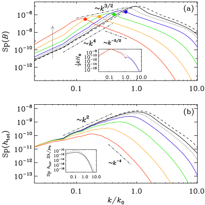
Figure 1: (a) Magnetic energy and (b) total helicity variance spectra at $t=31$ (dashed), $100$ (solid), $316$ (dotted), $10^{3}$ (blue), $3.16\times 10^{3}$ (green), $10^{4}$ (orange), and $3.16\times 10^{4}$ (red). In (a), note that $\mbox{\rm Sp}(\bm{B})$ evolves underneath the envelope $k^{3/2}$, and the upward arrow indicates the sense of time. For orientation, the slopes $k^{-5/2}$ and $k^{-4}$ have been indicated in what is expected to correspond to the inertial ranges in (a) and (b), respectively. In (a), the inset shows $(k/2)\,H_{\rm M}(k)$ at the last time with positive (negative) values in red (blue), and in (b), the inset compares $\mbox{\rm Sp}(2\mu_{5}/\lambda)$ (solid) with $\mbox{\rm Sp}(h_{\rm tot})$ (dotted) at the last time.

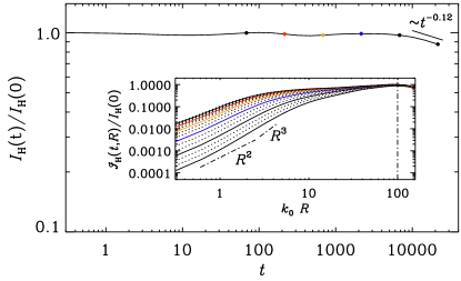
Figure 2: $I_{\rm H}(t)$ normalized by its initial value. The inset shows ${\cal I}_{\rm H}(R,t)$ versus $R$ at different times $t$: solid lines correspond to $t=70$, 200, 700, 2000, 7000, and 20,000, which are also marked by selected colored symbols in the graph of $I_{\rm H}(t)$. The adapted Hosking integral is evaluated as $I_{\rm H}(t)={\cal I}_{\rm H}(R_{*},t)$. The vertical dashed-dotted line marks the value $k_{0}R_{*}=100$ where the curves show a plateau. The slopes $\propto R^{2}$ and $\propto R^{3}$ are also marked by dashed-dotted lines.

To compute ${\cal I}_{\rm H}$ (and thereby $I_{\rm H}$), we employ a spectral technique by computing the total helicity variance spectrum $\mbox{\rm Sp}(h_{\rm tot})$; see Fig. 1(b). Compared to the inverse cascade seen in $\mbox{\rm Sp}(\bm{B})$, here we see the conservation of the large-scale total helicity variance spectrum $\propto k^{2}$. We thus obtain

$${\cal I}_{H}(R,t)=L^{-3}\int w(\bm{k},R)\,\mbox{\rm Sp}(h_{\rm tot})\,{\rm d}{}^{3}\bm{k}/(2\pi)^{3}.$$ (6)

We choose $w(k,R)=(4\pi R^{3}/3)[6j_{1}(kR)/kR]^{2}$ as weight function (Zhou et al., 2022) with $j_{n}$ being spherical Bessel functions.

In Fig. 2, we plot the adapted Hosking integral $I_{\rm H}(t)$, normalized by its initial value. It is evaluated as $I_{\rm H}(t)={\cal I}_{\rm H}(R_{*},t)$ with $k_{0}R_{*}=100$, where ${\cal I}_{\rm H}(R,t)$ is shown in the inset at different times as functions of $R$. Note that $I_{\rm H}(t)$ is essentially flat and shows only toward the end a slight decline $\propto t^{-0.12}$, which is similar to what has been seen for other simulations at that resolution; see, e.g., Ref. Brandenburg (2023). Thus, the adapted Hosking integral appears to be well conserved – even better so than the Hosking integral in ordinary MHD, studied in Refs. (Hosking and Schekochihin, 2021; Zhou et al., 2022). There is not even the slight uprise $I_{\rm H}(t)$ reported in Ref. (Zhou et al., 2022), which was there argued to be due to strong non-Gaussian contributions to the field that emerged during the nonlinear evolution of the system. Note also that for $R\ll R_{*}$, we see ${\cal I}_{\rm H}(R,t)\propto R^{2}$, which is shallower than the expected cubic scaling. This might change at larger resolution, although an intermediate range $\propto R^{2}$ is also seen in Fig. 4(d) of Ref. (Zhou et al., 2022), before cubic scaling emerged for $R/2\pi<10^{-4}$.

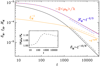
Figure 3: Time dependence of ${\cal E}_{\rm M}$ (black), $\xi_{\rm M}$ (orange), ${\cal H}_{\rm M}$ (blue), and $-2\langle\mu_{5}\rangle/\lambda$ (red). The inset confirms that $2{\cal E}_{\rm M}\xi_{\rm M}/{\cal H}_{\rm M}\approx 1$ during the whole time.

As in the case of nonrelativistic MHD ($\mu_{5}\to 0$), the dimensions of ${\cal I}_{\rm H}$ and $I_{\rm H}$ are $\,{\rm cm}^{9}\,{\rm s}^{-4}$. This implies that in $\xi_{\rm M}\propto t^{q}$, the value of the exponent is $q=4/9$, if the conservation of ${\cal I}_{\rm H}$ determines the time evolution of the magnetic field around the characteristic scale. Next, assuming selfsimilarity, the magnetic spectra can be collapsed on top of each other by plotting them versus $k\xi_{\rm M}(t)$ and compensating the decline in the height by $\xi_{\rm M}^{\beta}$ to yield the universal function $\phi(k\xi_{\rm M})=\xi_{\rm M}^{\beta}E_{\rm M}(k\xi_{\rm M})$; see Appendix B of Ref. Zhou et al. (2022) and Refs. Brandenburg and Kahniashvili (2017); Brandenburg (2023) for examples in other contexts. Using also the invariance of the spectrum under rescaling (Olesen, 1997), $\bm{x}\to\bm{x}^{\prime}=\bm{x}\ell$ and $t\to t^{\prime}=t\ell^{1/q}$, and since the dimension of $E_{\rm M}(k,t)$ is $\,{\rm cm}^{3}\,{\rm s}^{-2}$, we have $E_{\rm M}(k\ell^{-1},t\ell^{1/q})=\ell^{3-2/q+\beta}[\xi_{\rm M}\ell]^{-\beta}\phi(k\xi_{\rm M})$, and therefore $\beta=2/q-3=3/2$, which agrees with Fig. 1(a). Finally, for ${\cal E}_{\rm M}\propto t^{-p}$, we find with ${\cal E}_{\rm M}(t)=\int E_{\rm M}\,{\rm d}{}k\propto t^{-(\beta+1)q}$ the line $p=2(1-q)$, which is also known as the self-similarity line (Brandenburg and Kahniashvili, 2017; Zhou et al., 2022). With $q=4/9$, we thus obtain $p=10/9$. This is completely analogous to the MHD case with zero magnetic helicity; see also Table 2 of Ref. Brandenburg (2023). Thus, the cancellation of finite magnetic helicity by fermion chirality with ${\cal H}_{\rm M}(t)=-2\langle\mu_{5}\rangle(t)/\lambda\neq 0$ has the same effect as that of zero magnetic helicity.

To understand the decay of magnetic helicity density in the present simulations, it is important to remember that the real space realizability condition of magnetic helicity (Kahniashvili et al., 2013) is always valid and implies $|{\cal H}_{\rm M}|\leq 2{\cal E}_{\rm M}\xi_{\rm M}$. Assuming the inequality to be saturated, we find the scaling $|{\cal H}_{\rm M}|\propto|\langle\mu_{5}\rangle|\propto t^{-r}$ with $r=p-q=2/3$. This is well obeyed, as is shown in Fig. 3. In the inset, we show that $2{\cal E}_{\rm M}\xi_{\rm M}/{\cal H}_{\rm M}\approx 1$ at early times and about 1.1 at late times. It is thus fairly constant, therefore confirming the validity of our underlying assumption. On top of this evolution of the chiral asymmetry, the growth rate of the CPI, $\gamma_{5}\propto\langle\mu_{5}\rangle^{2}\propto t^{-4/3}$, decays more rapidly than $t^{-1}$, which causes it to grow less efficiently so as not to spoil the scaling properties of the system.

To characterize the scaling expected from the conservation of the adapted Hosking integral further, in Fig. 4 we plot the $pq$ diagram of the instantaneous scaling exponents $p(t)=-{\rm d}{}\ln{\cal E}_{\rm M}/{\rm d}{}\ln t$ versus $q(t)={\rm d}{}\ln\xi_{\rm M}/{\rm d}{}\ln t$. The solution converges to a point close to the crossing point between the $\beta=3/2$ line and the scale-invariance line $p=2(1-q)$. The approach to the point $(p,q)=(10/9,\,4/9)$ does not occur predominantly along the $\beta=3/2$ line, as in nonhelical standard MHD, but is now closer to the $r=2/3$ line, where $p=q+r$. In the unbalanced case, where the net chirality is non-vanishing, however, the decay is solely governed by $\langle h_{\rm tot}\rangle={\rm const}{}$ Brandenburg et al. (2023).

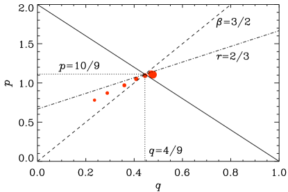
Figure 4: $pq$ diagram for times $t=700$, 1000, 1500, 2200, 3200, 4600, 6800, $10^{4}$, $1.5\times 10^{4}$, $1.5\times 10^{4}$, $2.2\times 10^{4}$, and $3.2\times 10^{4}$, corresponding to symbols of increasing size. The solid line denotes the scale-invariance line $p=2(1-q)$, the dashed line the $\beta=3/2$ line for adapted Hosking scaling, and the dashed-dotted line is the new $r=2/3$ line that does not have any correspondence in standard MHD.

In conclusion, we have presented evidence that, in the balanced case of zero total chirality, the Hosking integral, when adapted to include the chiral chemical potential, is approximately conserved around the characteristic scale. This implies decay properties for magnetic energy and correlation length that are unchanged relative to nonhelical MHD, but here with ${\cal H}_{\rm M}+2\langle\mu_{5}\rangle/\lambda=0$ (instead of ${\cal H}_{\rm M}=0$). This yields the scaling $|{\cal H}_{\rm M}|\propto|\langle\mu_{5}\rangle|\propto t^{-2/3}$, along with the familiar scalings ${\cal E}_{\rm M}\propto t^{-10/9}$ and $\xi_{\rm M}\propto t^{4/9}$ that also apply to the case with ${\cal H}_{\rm M}=0$. These scalings have consequences for understanding the properties of the chiral magnetic effect in the early Universe (Kamada, 2018; Del Zanna and Bucciantini, 2018; Domcke and Mukaida, 2018; Domcke et al., 2019, 2023) and young neutron stars (Masada et al., 2018; Dvornikov et al., 2020). Our work has significant impact on the baryon asymmetry of the Universe from hypermagnetic helicity decay after axion inflation. It also exposes a rather unexpected application of the general idea behind the recently developed Hosking integral, raising therefore the hope that there may be other ones yet to be discovered.